hypothesis template biology

Have a language expert improve your writing

Run a free plagiarism check in 10 minutes, automatically generate references for free.

• Knowledge Base
• Methodology
• How to Write a Strong Hypothesis | Guide & Examples

How to Write a Strong Hypothesis | Guide & Examples

Published on 6 May 2022 by Shona McCombes .

A hypothesis is a statement that can be tested by scientific research. If you want to test a relationship between two or more variables, you need to write hypotheses before you start your experiment or data collection.

Table of contents

What is a hypothesis, developing a hypothesis (with example), hypothesis examples, frequently asked questions about writing hypotheses.

A hypothesis states your predictions about what your research will find. It is a tentative answer to your research question that has not yet been tested. For some research projects, you might have to write several hypotheses that address different aspects of your research question.

A hypothesis is not just a guess – it should be based on existing theories and knowledge. It also has to be testable, which means you can support or refute it through scientific research methods (such as experiments, observations, and statistical analysis of data).

Variables in hypotheses

Hypotheses propose a relationship between two or more variables . An independent variable is something the researcher changes or controls. A dependent variable is something the researcher observes and measures.

In this example, the independent variable is exposure to the sun – the assumed cause . The dependent variable is the level of happiness – the assumed effect .

Prevent plagiarism, run a free check.

Step 1: ask a question.

Writing a hypothesis begins with a research question that you want to answer. The question should be focused, specific, and researchable within the constraints of your project.

Step 2: Do some preliminary research

Your initial answer to the question should be based on what is already known about the topic. Look for theories and previous studies to help you form educated assumptions about what your research will find.

At this stage, you might construct a conceptual framework to identify which variables you will study and what you think the relationships are between them. Sometimes, you’ll have to operationalise more complex constructs.

Step 3: Formulate your hypothesis

Now you should have some idea of what you expect to find. Write your initial answer to the question in a clear, concise sentence.

Step 4: Refine your hypothesis

You need to make sure your hypothesis is specific and testable. There are various ways of phrasing a hypothesis, but all the terms you use should have clear definitions, and the hypothesis should contain:

• The relevant variables
• The specific group being studied
• The predicted outcome of the experiment or analysis

Step 5: Phrase your hypothesis in three ways

To identify the variables, you can write a simple prediction in if … then form. The first part of the sentence states the independent variable and the second part states the dependent variable.

In academic research, hypotheses are more commonly phrased in terms of correlations or effects, where you directly state the predicted relationship between variables.

If you are comparing two groups, the hypothesis can state what difference you expect to find between them.

Step 6. Write a null hypothesis

If your research involves statistical hypothesis testing , you will also have to write a null hypothesis. The null hypothesis is the default position that there is no association between the variables. The null hypothesis is written as H 0 , while the alternative hypothesis is H 1 or H a .

Hypothesis testing is a formal procedure for investigating our ideas about the world using statistics. It is used by scientists to test specific predictions, called hypotheses , by calculating how likely it is that a pattern or relationship between variables could have arisen by chance.

A hypothesis is not just a guess. It should be based on existing theories and knowledge. It also has to be testable, which means you can support or refute it through scientific research methods (such as experiments, observations, and statistical analysis of data).

A research hypothesis is your proposed answer to your research question. The research hypothesis usually includes an explanation (‘ x affects y because …’).

A statistical hypothesis, on the other hand, is a mathematical statement about a population parameter. Statistical hypotheses always come in pairs: the null and alternative hypotheses. In a well-designed study , the statistical hypotheses correspond logically to the research hypothesis.

Cite this Scribbr article

If you want to cite this source, you can copy and paste the citation or click the ‘Cite this Scribbr article’ button to automatically add the citation to our free Reference Generator.

McCombes, S. (2022, May 06). How to Write a Strong Hypothesis | Guide & Examples. Scribbr. Retrieved 3 June 2024, from https://www.scribbr.co.uk/research-methods/hypothesis-writing/

Is this article helpful?

Shona McCombes

Other students also liked, operationalisation | a guide with examples, pros & cons, what is a conceptual framework | tips & examples, a quick guide to experimental design | 5 steps & examples.

Module 1: Introduction to Biology

Experiments and hypotheses, learning outcomes.

• Form a hypothesis and use it to design a scientific experiment

Now we’ll focus on the methods of scientific inquiry. Science often involves making observations and developing hypotheses. Experiments and further observations are often used to test the hypotheses.

A scientific experiment is a carefully organized procedure in which the scientist intervenes in a system to change something, then observes the result of the change. Scientific inquiry often involves doing experiments, though not always. For example, a scientist studying the mating behaviors of ladybugs might begin with detailed observations of ladybugs mating in their natural habitats. While this research may not be experimental, it is scientific: it involves careful and verifiable observation of the natural world. The same scientist might then treat some of the ladybugs with a hormone hypothesized to trigger mating and observe whether these ladybugs mated sooner or more often than untreated ones. This would qualify as an experiment because the scientist is now making a change in the system and observing the effects.

Forming a Hypothesis

When conducting scientific experiments, researchers develop hypotheses to guide experimental design. A hypothesis is a suggested explanation that is both testable and falsifiable. You must be able to test your hypothesis through observations and research, and it must be possible to prove your hypothesis false.

For example, Michael observes that maple trees lose their leaves in the fall. He might then propose a possible explanation for this observation: “cold weather causes maple trees to lose their leaves in the fall.” This statement is testable. He could grow maple trees in a warm enclosed environment such as a greenhouse and see if their leaves still dropped in the fall. The hypothesis is also falsifiable. If the leaves still dropped in the warm environment, then clearly temperature was not the main factor in causing maple leaves to drop in autumn.

In the Try It below, you can practice recognizing scientific hypotheses. As you consider each statement, try to think as a scientist would: can I test this hypothesis with observations or experiments? Is the statement falsifiable? If the answer to either of these questions is “no,” the statement is not a valid scientific hypothesis.

Practice Questions

Determine whether each following statement is a scientific hypothesis.

Air pollution from automobile exhaust can trigger symptoms in people with asthma.

• No. This statement is not testable or falsifiable.
• No. This statement is not testable.
• No. This statement is not falsifiable.
• Yes. This statement is testable and falsifiable.

Natural disasters, such as tornadoes, are punishments for bad thoughts and behaviors.

a: No. This statement is not testable or falsifiable. “Bad thoughts and behaviors” are excessively vague and subjective variables that would be impossible to measure or agree upon in a reliable way. The statement might be “falsifiable” if you came up with a counterexample: a “wicked” place that was not punished by a natural disaster. But some would question whether the people in that place were really wicked, and others would continue to predict that a natural disaster was bound to strike that place at some point. There is no reason to suspect that people’s immoral behavior affects the weather unless you bring up the intervention of a supernatural being, making this idea even harder to test.

Testing a Vaccine

Let’s examine the scientific process by discussing an actual scientific experiment conducted by researchers at the University of Washington. These researchers investigated whether a vaccine may reduce the incidence of the human papillomavirus (HPV). The experimental process and results were published in an article titled, “ A controlled trial of a human papillomavirus type 16 vaccine .”

Preliminary observations made by the researchers who conducted the HPV experiment are listed below:

• Human papillomavirus (HPV) is the most common sexually transmitted virus in the United States.
• There are about 40 different types of HPV. A significant number of people that have HPV are unaware of it because many of these viruses cause no symptoms.
• Some types of HPV can cause cervical cancer.
• About 4,000 women a year die of cervical cancer in the United States.

Practice Question

Researchers have developed a potential vaccine against HPV and want to test it. What is the first testable hypothesis that the researchers should study?

• HPV causes cervical cancer.
• People should not have unprotected sex with many partners.
• People who get the vaccine will not get HPV.
• The HPV vaccine will protect people against cancer.

Experimental Design

You’ve successfully identified a hypothesis for the University of Washington’s study on HPV: People who get the HPV vaccine will not get HPV.

The next step is to design an experiment that will test this hypothesis. There are several important factors to consider when designing a scientific experiment. First, scientific experiments must have an experimental group. This is the group that receives the experimental treatment necessary to address the hypothesis.

The experimental group receives the vaccine, but how can we know if the vaccine made a difference? Many things may change HPV infection rates in a group of people over time. To clearly show that the vaccine was effective in helping the experimental group, we need to include in our study an otherwise similar control group that does not get the treatment. We can then compare the two groups and determine if the vaccine made a difference. The control group shows us what happens in the absence of the factor under study.

However, the control group cannot get “nothing.” Instead, the control group often receives a placebo. A placebo is a procedure that has no expected therapeutic effect—such as giving a person a sugar pill or a shot containing only plain saline solution with no drug. Scientific studies have shown that the “placebo effect” can alter experimental results because when individuals are told that they are or are not being treated, this knowledge can alter their actions or their emotions, which can then alter the results of the experiment.

Moreover, if the doctor knows which group a patient is in, this can also influence the results of the experiment. Without saying so directly, the doctor may show—through body language or other subtle cues—their views about whether the patient is likely to get well. These errors can then alter the patient’s experience and change the results of the experiment. Therefore, many clinical studies are “double blind.” In these studies, neither the doctor nor the patient knows which group the patient is in until all experimental results have been collected.

Both placebo treatments and double-blind procedures are designed to prevent bias. Bias is any systematic error that makes a particular experimental outcome more or less likely. Errors can happen in any experiment: people make mistakes in measurement, instruments fail, computer glitches can alter data. But most such errors are random and don’t favor one outcome over another. Patients’ belief in a treatment can make it more likely to appear to “work.” Placebos and double-blind procedures are used to level the playing field so that both groups of study subjects are treated equally and share similar beliefs about their treatment.

The scientists who are researching the effectiveness of the HPV vaccine will test their hypothesis by separating 2,392 young women into two groups: the control group and the experimental group. Answer the following questions about these two groups.

• This group is given a placebo.
• This group is deliberately infected with HPV.
• This group is given nothing.
• This group is given the HPV vaccine.
• a: This group is given a placebo. A placebo will be a shot, just like the HPV vaccine, but it will have no active ingredient. It may change peoples’ thinking or behavior to have such a shot given to them, but it will not stimulate the immune systems of the subjects in the same way as predicted for the vaccine itself.
• d: This group is given the HPV vaccine. The experimental group will receive the HPV vaccine and researchers will then be able to see if it works, when compared to the control group.

Experimental Variables

A variable is a characteristic of a subject (in this case, of a person in the study) that can vary over time or among individuals. Sometimes a variable takes the form of a category, such as male or female; often a variable can be measured precisely, such as body height. Ideally, only one variable is different between the control group and the experimental group in a scientific experiment. Otherwise, the researchers will not be able to determine which variable caused any differences seen in the results. For example, imagine that the people in the control group were, on average, much more sexually active than the people in the experimental group. If, at the end of the experiment, the control group had a higher rate of HPV infection, could you confidently determine why? Maybe the experimental subjects were protected by the vaccine, but maybe they were protected by their low level of sexual contact.

To avoid this situation, experimenters make sure that their subject groups are as similar as possible in all variables except for the variable that is being tested in the experiment. This variable, or factor, will be deliberately changed in the experimental group. The one variable that is different between the two groups is called the independent variable. An independent variable is known or hypothesized to cause some outcome. Imagine an educational researcher investigating the effectiveness of a new teaching strategy in a classroom. The experimental group receives the new teaching strategy, while the control group receives the traditional strategy. It is the teaching strategy that is the independent variable in this scenario. In an experiment, the independent variable is the variable that the scientist deliberately changes or imposes on the subjects.

Dependent variables are known or hypothesized consequences; they are the effects that result from changes or differences in an independent variable. In an experiment, the dependent variables are those that the scientist measures before, during, and particularly at the end of the experiment to see if they have changed as expected. The dependent variable must be stated so that it is clear how it will be observed or measured. Rather than comparing “learning” among students (which is a vague and difficult to measure concept), an educational researcher might choose to compare test scores, which are very specific and easy to measure.

In any real-world example, many, many variables MIGHT affect the outcome of an experiment, yet only one or a few independent variables can be tested. Other variables must be kept as similar as possible between the study groups and are called control variables . For our educational research example, if the control group consisted only of people between the ages of 18 and 20 and the experimental group contained people between the ages of 30 and 35, we would not know if it was the teaching strategy or the students’ ages that played a larger role in the results. To avoid this problem, a good study will be set up so that each group contains students with a similar age profile. In a well-designed educational research study, student age will be a controlled variable, along with other possibly important factors like gender, past educational achievement, and pre-existing knowledge of the subject area.

What is the independent variable in this experiment?

• Sex (all of the subjects will be female)
• Presence or absence of the HPV vaccine
• Presence or absence of HPV (the virus)

List three control variables other than age.

What is the dependent variable in this experiment?

• Sex (male or female)
• Rates of HPV infection
• Age (years)
• Revision and adaptation. Authored by : Shelli Carter and Lumen Learning. Provided by : Lumen Learning. License : CC BY-NC-SA: Attribution-NonCommercial-ShareAlike
• Scientific Inquiry. Provided by : Open Learning Initiative. Located at : https://oli.cmu.edu/jcourse/workbook/activity/page?context=434a5c2680020ca6017c03488572e0f8 . Project : Introduction to Biology (Open + Free). License : CC BY-NC-SA: Attribution-NonCommercial-ShareAlike

• Science Notes Posts
• Contact Science Notes
• Todd Helmenstine Biography
• Anne Helmenstine Biography
• Free Printable Periodic Tables (PDF and PNG)
• Periodic Table Wallpapers
• Interactive Periodic Table
• Periodic Table Posters
• How to Grow Crystals
• Chemistry Projects
• Fire and Flames Projects
• Holiday Science
• Chemistry Problems With Answers
• Physics Problems
• Unit Conversion Example Problems
• Chemistry Worksheets
• Biology Worksheets
• Periodic Table Worksheets
• Physical Science Worksheets
• Science Lab Worksheets
• My Amazon Books

Hypothesis Examples

A hypothesis is a prediction of the outcome of a test. It forms the basis for designing an experiment in the scientific method . A good hypothesis is testable, meaning it makes a prediction you can check with observation or experimentation. Here are different hypothesis examples.

Null Hypothesis Examples

The null hypothesis (H 0 ) is also known as the zero-difference or no-difference hypothesis. It predicts that changing one variable ( independent variable ) will have no effect on the variable being measured ( dependent variable ). Here are null hypothesis examples:

• Plant growth is unaffected by temperature.
• If you increase temperature, then solubility of salt will increase.
• Incidence of skin cancer is unrelated to ultraviolet light exposure.
• All brands of light bulb last equally long.
• Cats have no preference for the color of cat food.
• All daisies have the same number of petals.

Sometimes the null hypothesis shows there is a suspected correlation between two variables. For example, if you think plant growth is affected by temperature, you state the null hypothesis: “Plant growth is not affected by temperature.” Why do you do this, rather than say “If you change temperature, plant growth will be affected”? The answer is because it’s easier applying a statistical test that shows, with a high level of confidence, a null hypothesis is correct or incorrect.

Research Hypothesis Examples

A research hypothesis (H 1 ) is a type of hypothesis used to design an experiment. This type of hypothesis is often written as an if-then statement because it’s easy identifying the independent and dependent variables and seeing how one affects the other. If-then statements explore cause and effect. In other cases, the hypothesis shows a correlation between two variables. Here are some research hypothesis examples:

• If you leave the lights on, then it takes longer for people to fall asleep.
• If you refrigerate apples, they last longer before going bad.
• If you keep the curtains closed, then you need less electricity to heat or cool the house (the electric bill is lower).
• If you leave a bucket of water uncovered, then it evaporates more quickly.
• Goldfish lose their color if they are not exposed to light.
• Workers who take vacations are more productive than those who never take time off.

Is It Okay to Disprove a Hypothesis?

Yes! You may even choose to write your hypothesis in such a way that it can be disproved because it’s easier to prove a statement is wrong than to prove it is right. In other cases, if your prediction is incorrect, that doesn’t mean the science is bad. Revising a hypothesis is common. It demonstrates you learned something you did not know before you conducted the experiment.

Test yourself with a Scientific Method Quiz .

• Mellenbergh, G.J. (2008). Chapter 8: Research designs: Testing of research hypotheses. In H.J. Adèr & G.J. Mellenbergh (eds.), Advising on Research Methods: A Consultant’s Companion . Huizen, The Netherlands: Johannes van Kessel Publishing.
• Popper, Karl R. (1959). The Logic of Scientific Discovery . Hutchinson & Co. ISBN 3-1614-8410-X.
• Schick, Theodore; Vaughn, Lewis (2002). How to think about weird things: critical thinking for a New Age . Boston: McGraw-Hill Higher Education. ISBN 0-7674-2048-9.
• Tobi, Hilde; Kampen, Jarl K. (2018). “Research design: the methodology for interdisciplinary research framework”. Quality & Quantity . 52 (3): 1209–1225. doi: 10.1007/s11135-017-0513-8

Related Posts

• Bipolar Disorder
• Therapy Center
• When To See a Therapist
• Types of Therapy
• Best Online Therapy
• Best Couples Therapy
• Best Family Therapy
• Managing Stress
• Sleep and Dreaming
• Understanding Emotions
• Self-Improvement
• Healthy Relationships
• Student Resources
• Personality Types
• Guided Meditations
• Verywell Mind Insights
• 2024 Verywell Mind 25
• Mental Health in the Classroom
• Editorial Process
• Meet Our Review Board
• Crisis Support

How to Write a Great Hypothesis

Hypothesis Definition, Format, Examples, and Tips

Kendra Cherry, MS, is a psychosocial rehabilitation specialist, psychology educator, and author of the "Everything Psychology Book."

Amy Morin, LCSW, is a psychotherapist and international bestselling author. Her books, including "13 Things Mentally Strong People Don't Do," have been translated into more than 40 languages. Her TEDx talk,  "The Secret of Becoming Mentally Strong," is one of the most viewed talks of all time.

Verywell / Alex Dos Diaz

• The Scientific Method

Hypothesis Format

Falsifiability of a hypothesis.

• Operationalization

Hypothesis Types

Hypotheses examples.

• Collecting Data

A hypothesis is a tentative statement about the relationship between two or more variables. It is a specific, testable prediction about what you expect to happen in a study. It is a preliminary answer to your question that helps guide the research process.

Consider a study designed to examine the relationship between sleep deprivation and test performance. The hypothesis might be: "This study is designed to assess the hypothesis that sleep-deprived people will perform worse on a test than individuals who are not sleep-deprived."

At a Glance

A hypothesis is crucial to scientific research because it offers a clear direction for what the researchers are looking to find. This allows them to design experiments to test their predictions and add to our scientific knowledge about the world. This article explores how a hypothesis is used in psychology research, how to write a good hypothesis, and the different types of hypotheses you might use.

The Hypothesis in the Scientific Method

In the scientific method , whether it involves research in psychology, biology, or some other area, a hypothesis represents what the researchers think will happen in an experiment. The scientific method involves the following steps:

• Forming a question
• Performing background research
• Creating a hypothesis
• Designing an experiment
• Collecting data
• Analyzing the results
• Drawing conclusions
• Communicating the results

The hypothesis is a prediction, but it involves more than a guess. Most of the time, the hypothesis begins with a question which is then explored through background research. At this point, researchers then begin to develop a testable hypothesis.

Unless you are creating an exploratory study, your hypothesis should always explain what you  expect  to happen.

In a study exploring the effects of a particular drug, the hypothesis might be that researchers expect the drug to have some type of effect on the symptoms of a specific illness. In psychology, the hypothesis might focus on how a certain aspect of the environment might influence a particular behavior.

Remember, a hypothesis does not have to be correct. While the hypothesis predicts what the researchers expect to see, the goal of the research is to determine whether this guess is right or wrong. When conducting an experiment, researchers might explore numerous factors to determine which ones might contribute to the ultimate outcome.

In many cases, researchers may find that the results of an experiment  do not  support the original hypothesis. When writing up these results, the researchers might suggest other options that should be explored in future studies.

In many cases, researchers might draw a hypothesis from a specific theory or build on previous research. For example, prior research has shown that stress can impact the immune system. So a researcher might hypothesize: "People with high-stress levels will be more likely to contract a common cold after being exposed to the virus than people who have low-stress levels."

In other instances, researchers might look at commonly held beliefs or folk wisdom. "Birds of a feather flock together" is one example of folk adage that a psychologist might try to investigate. The researcher might pose a specific hypothesis that "People tend to select romantic partners who are similar to them in interests and educational level."

Elements of a Good Hypothesis

So how do you write a good hypothesis? When trying to come up with a hypothesis for your research or experiments, ask yourself the following questions:

• Is your hypothesis based on your research on a topic?
• Can your hypothesis be tested?
• Does your hypothesis include independent and dependent variables?

Before you come up with a specific hypothesis, spend some time doing background research. Once you have completed a literature review, start thinking about potential questions you still have. Pay attention to the discussion section in the  journal articles you read . Many authors will suggest questions that still need to be explored.

How to Formulate a Good Hypothesis

To form a hypothesis, you should take these steps:

• Collect as many observations about a topic or problem as you can.
• Evaluate these observations and look for possible causes of the problem.
• Create a list of possible explanations that you might want to explore.
• After you have developed some possible hypotheses, think of ways that you could confirm or disprove each hypothesis through experimentation. This is known as falsifiability.

In the scientific method ,  falsifiability is an important part of any valid hypothesis. In order to test a claim scientifically, it must be possible that the claim could be proven false.

Students sometimes confuse the idea of falsifiability with the idea that it means that something is false, which is not the case. What falsifiability means is that  if  something was false, then it is possible to demonstrate that it is false.

One of the hallmarks of pseudoscience is that it makes claims that cannot be refuted or proven false.

The Importance of Operational Definitions

A variable is a factor or element that can be changed and manipulated in ways that are observable and measurable. However, the researcher must also define how the variable will be manipulated and measured in the study.

Operational definitions are specific definitions for all relevant factors in a study. This process helps make vague or ambiguous concepts detailed and measurable.

For example, a researcher might operationally define the variable " test anxiety " as the results of a self-report measure of anxiety experienced during an exam. A "study habits" variable might be defined by the amount of studying that actually occurs as measured by time.

These precise descriptions are important because many things can be measured in various ways. Clearly defining these variables and how they are measured helps ensure that other researchers can replicate your results.

Replicability

One of the basic principles of any type of scientific research is that the results must be replicable.

Replication means repeating an experiment in the same way to produce the same results. By clearly detailing the specifics of how the variables were measured and manipulated, other researchers can better understand the results and repeat the study if needed.

Some variables are more difficult than others to define. For example, how would you operationally define a variable such as aggression ? For obvious ethical reasons, researchers cannot create a situation in which a person behaves aggressively toward others.

To measure this variable, the researcher must devise a measurement that assesses aggressive behavior without harming others. The researcher might utilize a simulated task to measure aggressiveness in this situation.

Hypothesis Checklist

• Does your hypothesis focus on something that you can actually test?
• Does your hypothesis include both an independent and dependent variable?
• Can you manipulate the variables?
• Can your hypothesis be tested without violating ethical standards?

The hypothesis you use will depend on what you are investigating and hoping to find. Some of the main types of hypotheses that you might use include:

• Simple hypothesis : This type of hypothesis suggests there is a relationship between one independent variable and one dependent variable.
• Complex hypothesis : This type suggests a relationship between three or more variables, such as two independent and dependent variables.
• Null hypothesis : This hypothesis suggests no relationship exists between two or more variables.
• Alternative hypothesis : This hypothesis states the opposite of the null hypothesis.
• Statistical hypothesis : This hypothesis uses statistical analysis to evaluate a representative population sample and then generalizes the findings to the larger group.
• Logical hypothesis : This hypothesis assumes a relationship between variables without collecting data or evidence.

A hypothesis often follows a basic format of "If {this happens} then {this will happen}." One way to structure your hypothesis is to describe what will happen to the  dependent variable  if you change the  independent variable .

The basic format might be: "If {these changes are made to a certain independent variable}, then we will observe {a change in a specific dependent variable}."

A few examples of simple hypotheses:

• "Students who eat breakfast will perform better on a math exam than students who do not eat breakfast."
• "Students who experience test anxiety before an English exam will get lower scores than students who do not experience test anxiety."​
• "Motorists who talk on the phone while driving will be more likely to make errors on a driving course than those who do not talk on the phone."
• "Children who receive a new reading intervention will have higher reading scores than students who do not receive the intervention."

Examples of a complex hypothesis include:

• "People with high-sugar diets and sedentary activity levels are more likely to develop depression."
• "Younger people who are regularly exposed to green, outdoor areas have better subjective well-being than older adults who have limited exposure to green spaces."

Examples of a null hypothesis include:

• "There is no difference in anxiety levels between people who take St. John's wort supplements and those who do not."
• "There is no difference in scores on a memory recall task between children and adults."
• "There is no difference in aggression levels between children who play first-person shooter games and those who do not."

Examples of an alternative hypothesis:

• "People who take St. John's wort supplements will have less anxiety than those who do not."
• "Adults will perform better on a memory task than children."
• "Children who play first-person shooter games will show higher levels of aggression than children who do not." 

Collecting Data on Your Hypothesis

Once a researcher has formed a testable hypothesis, the next step is to select a research design and start collecting data. The research method depends largely on exactly what they are studying. There are two basic types of research methods: descriptive research and experimental research.

Descriptive Research Methods

Descriptive research such as  case studies ,  naturalistic observations , and surveys are often used when  conducting an experiment is difficult or impossible. These methods are best used to describe different aspects of a behavior or psychological phenomenon.

Once a researcher has collected data using descriptive methods, a  correlational study  can examine how the variables are related. This research method might be used to investigate a hypothesis that is difficult to test experimentally.

Experimental Research Methods

Experimental methods  are used to demonstrate causal relationships between variables. In an experiment, the researcher systematically manipulates a variable of interest (known as the independent variable) and measures the effect on another variable (known as the dependent variable).

Unlike correlational studies, which can only be used to determine if there is a relationship between two variables, experimental methods can be used to determine the actual nature of the relationship—whether changes in one variable actually  cause  another to change.

The hypothesis is a critical part of any scientific exploration. It represents what researchers expect to find in a study or experiment. In situations where the hypothesis is unsupported by the research, the research still has value. Such research helps us better understand how different aspects of the natural world relate to one another. It also helps us develop new hypotheses that can then be tested in the future.

Thompson WH, Skau S. On the scope of scientific hypotheses .  R Soc Open Sci . 2023;10(8):230607. doi:10.1098/rsos.230607

Taran S, Adhikari NKJ, Fan E. Falsifiability in medicine: what clinicians can learn from Karl Popper [published correction appears in Intensive Care Med. 2021 Jun 17;:].  Intensive Care Med . 2021;47(9):1054-1056. doi:10.1007/s00134-021-06432-z

Eyler AA. Research Methods for Public Health . 1st ed. Springer Publishing Company; 2020. doi:10.1891/9780826182067.0004

Nosek BA, Errington TM. What is replication ?  PLoS Biol . 2020;18(3):e3000691. doi:10.1371/journal.pbio.3000691

Aggarwal R, Ranganathan P. Study designs: Part 2 - Descriptive studies .  Perspect Clin Res . 2019;10(1):34-36. doi:10.4103/picr.PICR_154_18

Nevid J. Psychology: Concepts and Applications. Wadworth, 2013.

By Kendra Cherry, MSEd Kendra Cherry, MS, is a psychosocial rehabilitation specialist, psychology educator, and author of the "Everything Psychology Book."

Scientific Method: Step 3: HYPOTHESIS

• Step 1: QUESTION
• Step 2: RESEARCH
• Step 3: HYPOTHESIS
• Step 4: EXPERIMENT
• Step 5: DATA
• Step 6: CONCLUSION

Step 3: State your hypothesis

Now it's time to state your hypothesis . The hypothesis is an educated guess as to what will happen during your experiment. 

The hypothesis is often written using the words "IF" and "THEN." For example, " If I do not study, then I will fail the test." The "if' and "then" statements reflect your independent and dependent variables . 

The hypothesis should relate back to your original question and must be testable .

A word about variables...

Your experiment will include variables to measure and to explain any cause and effect. Below you will find some useful links describing the different types of variables.

• "What are independent and dependent variables" NCES
• [VIDEO] Biology: Independent vs. Dependent Variables (Nucleus Medical Media) Video explaining independent and dependent variables, with examples.

Resource Links

• What is and How to Write a Good Hypothesis in Research? (Elsevier)
• Hypothesis brochure from Penn State/Berks

• << Previous: Step 2: RESEARCH
• Next: Step 4: EXPERIMENT >>
• Last Updated: May 9, 2024 10:59 AM
• URL: https://harford.libguides.com/scientific_method

Hypothesis Maker Online

Looking for a hypothesis maker? This online tool for students will help you formulate a beautiful hypothesis quickly, efficiently, and for free.

Are you looking for an effective hypothesis maker online? Worry no more; try our online tool for students and formulate your hypothesis within no time.

• 🔎 How to Use the Tool?
• ⚗️ What Is a Hypothesis in Science?

👍 What Does a Good Hypothesis Mean?

• 🧭 Steps to Making a Good Hypothesis

🔗 References

📄 hypothesis maker: how to use it.

Our hypothesis maker is a simple and efficient tool you can access online for free.

If you want to create a research hypothesis quickly, you should fill out the research details in the given fields on the hypothesis generator.

Below are the fields you should complete to generate your hypothesis:

• Who or what is your research based on? For instance, the subject can be research group 1.
• What does the subject (research group 1) do?
• What does the subject affect? - This shows the predicted outcome, which is the object.
• Who or what will be compared with research group 1? (research group 2).

Once you fill the in the fields, you can click the ‘Make a hypothesis’ tab and get your results.

⚗️ What Is a Hypothesis in the Scientific Method?

A hypothesis is a statement describing an expectation or prediction of your research through observation.

It is similar to academic speculation and reasoning that discloses the outcome of your scientific test . An effective hypothesis, therefore, should be crafted carefully and with precision.

A good hypothesis should have dependent and independent variables . These variables are the elements you will test in your research method – it can be a concept, an event, or an object as long as it is observable.

You can observe the dependent variables while the independent variables keep changing during the experiment.

In a nutshell, a hypothesis directs and organizes the research methods you will use, forming a large section of research paper writing.

Hypothesis vs. Theory

A hypothesis is a realistic expectation that researchers make before any investigation. It is formulated and tested to prove whether the statement is true. A theory, on the other hand, is a factual principle supported by evidence. Thus, a theory is more fact-backed compared to a hypothesis.

Another difference is that a hypothesis is presented as a single statement , while a theory can be an assortment of things . Hypotheses are based on future possibilities toward a specific projection, but the results are uncertain. Theories are verified with undisputable results because of proper substantiation.

When it comes to data, a hypothesis relies on limited information , while a theory is established on an extensive data set tested on various conditions.

You should observe the stated assumption to prove its accuracy.

Since hypotheses have observable variables, their outcome is usually based on a specific occurrence. Conversely, theories are grounded on a general principle involving multiple experiments and research tests.

This general principle can apply to many specific cases.

The primary purpose of formulating a hypothesis is to present a tentative prediction for researchers to explore further through tests and observations. Theories, in their turn, aim to explain plausible occurrences in the form of a scientific study.

It would help to rely on several criteria to establish a good hypothesis. Below are the parameters you should use to analyze the quality of your hypothesis.

🧭 6 Steps to Making a Good Hypothesis

Writing a hypothesis becomes way simpler if you follow a tried-and-tested algorithm. Let’s explore how you can formulate a good hypothesis in a few steps:

Step #1: Ask Questions

The first step in hypothesis creation is asking real questions about the surrounding reality.

Why do things happen as they do? What are the causes of some occurrences?

Your curiosity will trigger great questions that you can use to formulate a stellar hypothesis. So, ensure you pick a research topic of interest to scrutinize the world’s phenomena, processes, and events.

Step #2: Do Initial Research

Carry out preliminary research and gather essential background information about your topic of choice.

The extent of the information you collect will depend on what you want to prove.

Your initial research can be complete with a few academic books or a simple Internet search for quick answers with relevant statistics.

Still, keep in mind that in this phase, it is too early to prove or disapprove of your hypothesis.

Step #3: Identify Your Variables

Now that you have a basic understanding of the topic, choose the dependent and independent variables.

Take note that independent variables are the ones you can’t control, so understand the limitations of your test before settling on a final hypothesis.

Step #4: Formulate Your Hypothesis

You can write your hypothesis as an ‘if – then’ expression . Presenting any hypothesis in this format is reliable since it describes the cause-and-effect you want to test.

For instance: If I study every day, then I will get good grades.

Step #5: Gather Relevant Data

Once you have identified your variables and formulated the hypothesis, you can start the experiment. Remember, the conclusion you make will be a proof or rebuttal of your initial assumption.

So, gather relevant information, whether for a simple or statistical hypothesis, because you need to back your statement.

Step #6: Record Your Findings

Finally, write down your conclusions in a research paper .

Outline in detail whether the test has proved or disproved your hypothesis.

Edit and proofread your work, using a plagiarism checker to ensure the authenticity of your text.

We hope that the above tips will be useful for you. Note that if you need to conduct business analysis, you can use the free templates we’ve prepared: SWOT , PESTLE , VRIO , SOAR , and Porter’s 5 Forces .

❓ Hypothesis Formulator FAQ

Updated: Oct 25th, 2023

• How to Write a Hypothesis in 6 Steps - Grammarly
• Forming a Good Hypothesis for Scientific Research
• The Hypothesis in Science Writing
• Scientific Method: Step 3: HYPOTHESIS - Subject Guides
• Hypothesis Template & Examples - Video & Lesson Transcript
• Free Essays
• Writing Tools
• Lit. Guides
• Donate a Paper
• Referencing Guides
• Free Textbooks
• Tongue Twisters
• Job Openings
• Expert Application
• Video Contest
• Writing Scholarship
• Discount Codes
• IvyPanda Shop
• Terms and Conditions
• Privacy Policy
• Cookies Policy
• Copyright Principles
• DMCA Request
• Service Notice

Use our hypothesis maker whenever you need to formulate a hypothesis for your study. We offer a very simple tool where you just need to provide basic info about your variables, subjects, and predicted outcomes. The rest is on us. Get a perfect hypothesis in no time!

Want to create or adapt books like this? Learn more about how Pressbooks supports open publishing practices.

Biologists study the living world by posing questions about it and seeking science-based responses. This approach is common to other sciences as well and is often referred to as the scientific method . The scientific process was used even in ancient times, but it was first documented by England’s Sir Francis Bacon (1561–1626) ( Figure 1 ), who set up inductive methods for scientific inquiry. The scientific method is not exclusively used by biologists but can be applied to almost anything as a logical problem solving method.

The scientific process typically starts with an observation (often a problem to be solved) that leads to a question.  Remember that science is very good at answering questions having to do with observations about the natural world, but is very bad at answering questions having to do with morals, ethics, or personal opinions.

Let’s think about a simple problem that starts with an observation and apply the scientific method to solve the problem. Imagine that one morning when you wake up and flip a the switch to turn on your bedside lamp, the light won’t turn on. That is an observation that also describes a problem: the lights won’t turn on. Of course, you would next ask the question: “Why won’t the light turn on?”

Recall that a hypothesis is a suggested explanation that can be tested. A hypothesis is NOT the question you are trying to answer – it is what you think the answer to the question will be and why . To solve a problem, several hypotheses may be proposed. For example, one hypothesis might be, “The light won’t turn on because the bulb is burned out.” But there could be other answers to the question, and therefore other hypotheses may be proposed. A second hypothesis might be, “The light won’t turn on because the lamp is unplugged” or “The light won’t turn on because the power is out.” A hypothesis should be based on credible background information. A hypothesis is NOT just a guess (not even an educated one), although it can be based on your prior experience (such as in the example where the light won’t turn on). In general, hypotheses in biology should be based on a credible, referenced source of information.

A hypothesis must be testable  to ensure that it is valid. For example, a hypothesis that depends on what a dog thinks is not testable, because we can’t tell what a dog thinks. It should also be  falsifiable,  meaning that it can be disproven by experimental results. An example of an unfalsifiable hypothesis is “Red is a better color than blue.” There is no experiment that might show this statement to be false. To test a hypothesis, a researcher will conduct one or more experiments designed to eliminate one or more of the hypotheses. This is important: a hypothesis can be disproven, or eliminated, but it can never be proven. Science does not deal in proofs like mathematics. If an experiment fails to disprove a hypothesis, then that explanation (the hypothesis) is supported as the answer to the question. However, that doesn’t mean that later on, we won’t find a better explanation or design a better experiment that will be found to falsify the first hypothesis and lead to a better one.

A variable is any part of the experiment that can vary or change during the experiment. Typically, an experiment only tests one variable and all the other conditions in the experiment are held constant.

• The variable that is tested is known as the  independent variable .
• The  dependent variable  is the thing (or things) that you are measuring as the outcome of your experiment.
• A  constant  is a condition that is the same between all of the tested groups.
• A confounding variable is a condition that is not held constant that could affect the experimental results.

A hypothesis often has the format “If [I change the independent variable in this way] then [I will observe that the dependent variable does this] because [of some reason].” For example, the first hypothesis might be, “If you change the light bulb, then the light will turn on because the bulb is burned out.” In this experiment, the independent variable (the thing that you are testing) would be changing the light bulb and the dependent variable is whether or not the light turns on. It would be important to hold all the other aspects of the environment constant, for example not messing with the lamp cord or trying to turn the lamp on using a different light switch. If the entire house had lost power during the experiment because a car hit the power pole, that would be a confounding variable.

You may have learned that a hypothesis can be phrased as an “If..then…” statement. Simple hypotheses can be phrased that way (but they must also include a “because”), but more complicated hypotheses may require several sentences. It is also very easy to get confused by trying to put your hypothesis into this format. Hypotheses do not have to be phrased as “if..then..” statements, it is just sometimes a useful format.

The results of your experiment are the data that you collect as the outcome.  In the light experiment, your results are either that the light turns on or the light doesn’t turn on. Based on your results, you can make a conclusion. Your conclusion uses the results to answer your original question.

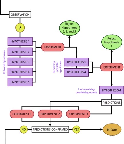
We can put the experiment with the light that won’t go in into the figure above:

• Observation: the light won’t turn on.
• Question: why won’t the light turn on?
• Hypothesis: the lightbulb is burned out.
• Prediction: if I change the lightbulb (independent variable), then the light will turn on (dependent variable).
• Experiment: change the lightbulb while leaving all other variables the same.
• Analyze the results: the light didn’t turn on.
• Conclusion: The lightbulb isn’t burned out. The results do not support the hypothesis, time to develop a new one!
• Hypothesis 2: the lamp is unplugged.
• Prediction 2: if I plug in the lamp, then the light will turn on.
• Experiment: plug in the lamp
• Analyze the results: the light turned on!
• Conclusion: The light wouldn’t turn on because the lamp was unplugged. The results support the hypothesis, it’s time to move on to the next experiment!

In practice, the scientific method is not as rigid and structured as it might at first appear. Sometimes an experiment leads to conclusions that favor a change in approach; often, an experiment brings entirely new scientific questions to the puzzle. Many times, science does not operate in a linear fashion; instead, scientists continually draw inferences and make generalizations, finding patterns as their research proceeds. Scientific reasoning is more complex than the scientific method alone suggests.

Control Groups

Another important aspect of designing an experiment is the presence of one or more control groups. A control group allows you to make a comparison that is important for interpreting your results. Control groups are samples that help you to determine that differences between your experimental groups are due to your treatment rather than a different variable – they eliminate alternate explanations for your results (including experimental error and experimenter bias). They increase reliability, often through the comparison of control measurements and measurements of the experimental groups. Often, the control group is a sample that is not treated with the independent variable, but is otherwise treated the same way as your experimental sample. This type of control group contains every feature of the experimental group except it is not given the manipulation that is hypothesized about (it does not get treated with the independent variable). Therefore, if the results of the experimental group differ from the control group, the difference must be due to the hypothesized manipulation, rather than some outside factor. It is common in complex experiments (such as those published in scientific journals) to have more control groups than experimental groups.

Question: Which fertilizer will produce the greatest number of tomatoes when applied to the plants?

Prediction and Hypothesis : If I apply different brands of fertilizer to tomato plants, the most tomatoes will be produced from plants watered with Brand A because Brand A advertises that it produces twice as many tomatoes as other leading brands.

Experiment: Purchase 10 tomato plants of the same type from the same nursery. Pick plants that are similar in size and age. Divide the plants into two groups of 5. Apply Brand A to the first group and Brand B to the second group according to the instructions on the packages. After 10 weeks, count the number of tomatoes on each plant.

Independent Variable: Brand of fertilizer.

Dependent Variable : Number of tomatoes.

The number of tomatoes produced depends on the brand of fertilizer applied to the plants.

Constants: amount of water, type of soil, size of pot, amount of light, type of tomato plant, length of time plants were grown.

Confounding variables : any of the above that are not held constant, plant health, diseases present in the soil or plant before it was purchased.

Results: Tomatoes fertilized with Brand A  produced an average of 20 tomatoes per plant, while tomatoes fertilized with Brand B produced an average of 10 tomatoes per plant.

You’d want to use Brand A next time you grow tomatoes, right? But what if I told you that plants grown without fertilizer produced an average of 30 tomatoes per plant! Now what will you use on your tomatoes?

Results including control group : Tomatoes which received no fertilizer produced more tomatoes than either brand of fertilizer.

Conclusion: Although Brand A fertilizer produced more tomatoes than Brand B, neither fertilizer should be used because plants grown without fertilizer produced the most tomatoes!

Positive control groups are often used to show that the experiment is valid and that everything has worked correctly. You can think of a positive control group as being a group where you should be able to observe the thing that you are measuring (“the thing” should happen). The conditions in a positive control group should guarantee a positive result. If the positive control group doesn’t work, there may be something wrong with the experimental procedure.

Negative control groups are used to show whether a treatment had any effect. If your treated sample is the same as your negative control group, your treatment had no effect. You can also think of a negative control group as being a group where you should NOT be able to observe the thing that you are measuring (“the thing” shouldn’t happen), or where you should not observe any change in the thing that you are measuring (there is no difference between the treated and control group). The conditions in a negative control group should guarantee a negative result. A placebo group is an example of a negative control group.

As a general rule, you need a positive control to validate a negative result, and a negative control to validate a positive result.

• You read an article in the NY Times that says some spinach is contaminated with Salmonella. You want to test the spinach you have at home in your fridge, so you wet a sterile swab and wipe it on the spinach, then wipe the swab on a nutrient plate (petri plate).
• You observe growth . Does this mean that your spinach is really contaminated? Consider an alternate explanation for growth: the swab, the water, or the plate is contaminated with bacteria. You could use a negative control to determine which explanation is true. If a swab is wet and wiped on a nutrient plate, do bacteria grow?
• You don’t observe growth. Does this mean that your spinach is really safe? Consider an alternate explanation for no growth: Salmonella isn’t able to grow on the type of nutrient you used in your plates. You could use a positive control to determine which explanation is true. If you wipe a known sample of Salmonella bacteria on the plate, do bacteria grow?
• In a drug trial, one group of subjects are given a new drug, while a second group is given a placebo drug  (a sugar pill; something which appears like the drug, but doesn’t contain the active ingredient). Reduction in disease symptoms are measured. The second group receiving the placebo is a negative control group. You might expect a reduction in disease symptoms purely because the person knows they are taking a drug so they should be getting better. If the group treated with the real drug does not show more a reduction in disease symptoms than the placebo group, the drug doesn’t really work. The placebo group sets a baseline against which the experimental group (treated with the drug) can be compared. A positive control group is not required for this experiment.
• In an experiment measuring the  preference of birds for various types of food , a negative control group would be a “placebo feeder”. This would be the same type of feeder, but with no food in it. Birds might visit a feeder just because they are interested in it; an empty feeder would give a baseline level for bird visits. A positive control group might be a food that squirrels are known to like. This would be useful because if no squirrels visited any of the feeders, you couldn’t tell if this was because there were no squirrels around or because they didn’t like any of your food offerings!
• To test  the effect of pH on the function of an enzyme , you would want a positive control group where you knew the enzyme would function (pH not changed) and a negative control group where you knew the enzyme would not function (no enzyme added). You need the positive control group so you know your enzyme is working: if you didn’t see a reaction in any of the tubes with the pH adjusted, you wouldn’t know if it was because the enzyme wasn’t working at all or because the enzyme just didn’t work at any of your tested pH. You need the negative control group so you can ensure that there is no reaction taking place in the absence of enzyme: if the reaction proceeds without the enzyme, your results are meaningless.

Text adapted from: OpenStax , Biology. OpenStax CNX. May 27, 2016  http://cnx.org/contents/[email protected]:RD6ERYiU@5/The-Process-of-Science .

MHCC Biology 112: Biology for Health Professions Copyright © 2019 by Lisa Bartee is licensed under a Creative Commons Attribution 4.0 International License , except where otherwise noted.

Share This Book

Hypothesis n., plural: hypotheses [/haɪˈpɑːθəsɪs/] Definition: Testable scientific prediction

Table of Contents

What Is Hypothesis?

A scientific hypothesis is a foundational element of the scientific method . It’s a testable statement proposing a potential explanation for natural phenomena. The term hypothesis means “little theory” . A hypothesis is a short statement that can be tested and gives a possible reason for a phenomenon or a possible link between two variables . In the setting of scientific research, a hypothesis is a tentative explanation or statement that can be proven wrong and is used to guide experiments and empirical research.

It is an important part of the scientific method because it gives a basis for planning tests, gathering data, and judging evidence to see if it is true and could help us understand how natural things work. Several hypotheses can be tested in the real world, and the results of careful and systematic observation and analysis can be used to support, reject, or improve them.

Researchers and scientists often use the word hypothesis to refer to this educated guess . These hypotheses are firmly established based on scientific principles and the rigorous testing of new technology and experiments .

For example, in astrophysics, the Big Bang Theory is a working hypothesis that explains the origins of the universe and considers it as a natural phenomenon. It is among the most prominent scientific hypotheses in the field.

“The scientific method: steps, terms, and examples” by Scishow:

Biology definition: A hypothesis  is a supposition or tentative explanation for (a group of) phenomena, (a set of) facts, or a scientific inquiry that may be tested, verified or answered by further investigation or methodological experiment. It is like a scientific guess . It’s an idea or prediction that scientists make before they do experiments. They use it to guess what might happen and then test it to see if they were right. It’s like a smart guess that helps them learn new things. A scientific hypothesis that has been verified through scientific experiment and research may well be considered a scientific theory .

Etymology: The word “hypothesis” comes from the Greek word “hupothesis,” which means “a basis” or “a supposition.” It combines “hupo” (under) and “thesis” (placing). Synonym:   proposition; assumption; conjecture; postulate Compare:   theory See also: null hypothesis

Characteristics Of Hypothesis

A useful hypothesis must have the following qualities:

• It should never be written as a question.
• You should be able to test it in the real world to see if it’s right or wrong.
• It needs to be clear and exact.
• It should list the factors that will be used to figure out the relationship.
• It should only talk about one thing. You can make a theory in either a descriptive or form of relationship.
• It shouldn’t go against any natural rule that everyone knows is true. Verification will be done well with the tools and methods that are available.
• It should be written in as simple a way as possible so that everyone can understand it.
• It must explain what happened to make an answer necessary.
• It should be testable in a fair amount of time.
• It shouldn’t say different things.

Sources Of Hypothesis

Sources of hypothesis are:

• Patterns of similarity between the phenomenon under investigation and existing hypotheses.
• Insights derived from prior research, concurrent observations, and insights from opposing perspectives.
• The formulations are derived from accepted scientific theories and proposed by researchers.
• In research, it’s essential to consider hypothesis as different subject areas may require various hypotheses (plural form of hypothesis). Researchers also establish a significance level to determine the strength of evidence supporting a hypothesis.
• Individual cognitive processes also contribute to the formation of hypotheses.

One hypothesis is a tentative explanation for an observation or phenomenon. It is based on prior knowledge and understanding of the world, and it can be tested by gathering and analyzing data. Observed facts are the data that are collected to test a hypothesis. They can support or refute the hypothesis.

For example, the hypothesis that “eating more fruits and vegetables will improve your health” can be tested by gathering data on the health of people who eat different amounts of fruits and vegetables. If the people who eat more fruits and vegetables are healthier than those who eat less fruits and vegetables, then the hypothesis is supported.

Hypotheses are essential for scientific inquiry. They help scientists to focus their research, to design experiments, and to interpret their results. They are also essential for the development of scientific theories.

Types Of Hypothesis

In research, you typically encounter two types of hypothesis: the alternative hypothesis (which proposes a relationship between variables) and the null hypothesis (which suggests no relationship).

Simple Hypothesis

It illustrates the association between one dependent variable and one independent variable. For instance, if you consume more vegetables, you will lose weight more quickly. Here, increasing vegetable consumption is the independent variable, while weight loss is the dependent variable.

Complex Hypothesis

It exhibits the relationship between at least two dependent variables and at least two independent variables. Eating more vegetables and fruits results in weight loss, radiant skin, and a decreased risk of numerous diseases, including heart disease.

Directional Hypothesis

It shows that a researcher wants to reach a certain goal. The way the factors are related can also tell us about their nature. For example, four-year-old children who eat well over a time of five years have a higher IQ than children who don’t eat well. This shows what happened and how it happened.

Non-directional Hypothesis

When there is no theory involved, it is used. It is a statement that there is a connection between two variables, but it doesn’t say what that relationship is or which way it goes.

Null Hypothesis

It says something that goes against the theory. It’s a statement that says something is not true, and there is no link between the independent and dependent factors. “H 0 ” represents the null hypothesis.

Associative and Causal Hypothesis

When a change in one variable causes a change in the other variable, this is called the associative hypothesis . The causal hypothesis, on the other hand, says that there is a cause-and-effect relationship between two or more factors.

Examples Of Hypothesis

Examples of simple hypotheses:

• Students who consume breakfast before taking a math test will have a better overall performance than students who do not consume breakfast.
• Students who experience test anxiety before an English examination will get lower scores than students who do not experience test anxiety.
• Motorists who talk on the phone while driving will be more likely to make errors on a driving course than those who do not talk on the phone, is a statement that suggests that drivers who talk on the phone while driving are more likely to make mistakes.

Examples of a complex hypothesis:

• Individuals who consume a lot of sugar and don’t get much exercise are at an increased risk of developing depression.
• Younger people who are routinely exposed to green, outdoor areas have better subjective well-being than older adults who have limited exposure to green spaces, according to a new study.
• Increased levels of air pollution led to higher rates of respiratory illnesses, which in turn resulted in increased costs for healthcare for the affected communities.

Examples of Directional Hypothesis:

• The crop yield will go up a lot if the amount of fertilizer is increased.
• Patients who have surgery and are exposed to more stress will need more time to get better.
• Increasing the frequency of brand advertising on social media will lead to a significant increase in brand awareness among the target audience.

Examples of Non-Directional Hypothesis (or Two-Tailed Hypothesis):

• The test scores of two groups of students are very different from each other.
• There is a link between gender and being happy at work.
• There is a correlation between the amount of caffeine an individual consumes and the speed with which they react.

Examples of a null hypothesis:

• Children who receive a new reading intervention will have scores that are different than students who do not receive the intervention.
• The results of a memory recall test will not reveal any significant gap in performance between children and adults.
• There is not a significant relationship between the number of hours spent playing video games and academic performance.

Examples of Associative Hypothesis:

• There is a link between how many hours you spend studying and how well you do in school.
• Drinking sugary drinks is bad for your health as a whole.
• There is an association between socioeconomic status and access to quality healthcare services in urban neighborhoods.

Functions Of Hypothesis

The research issue can be understood better with the help of a hypothesis, which is why developing one is crucial. The following are some of the specific roles that a hypothesis plays: (Rashid, Apr 20, 2022)

• A hypothesis gives a study a point of concentration. It enlightens us as to the specific characteristics of a study subject we need to look into.
• It instructs us on what data to acquire as well as what data we should not collect, giving the study a focal point .
• The development of a hypothesis improves objectivity since it enables the establishment of a focal point.
• A hypothesis makes it possible for us to contribute to the development of the theory. Because of this, we are in a position to definitively determine what is true and what is untrue .

How will Hypothesis help in the Scientific Method?

• The scientific method begins with observation and inquiry about the natural world when formulating research questions. Researchers can refine their observations and queries into specific, testable research questions with the aid of hypothesis. They provide an investigation with a focused starting point.
• Hypothesis generate specific predictions regarding the expected outcomes of experiments or observations. These forecasts are founded on the researcher’s current knowledge of the subject. They elucidate what researchers anticipate observing if the hypothesis is true.
• Hypothesis direct the design of experiments and data collection techniques. Researchers can use them to determine which variables to measure or manipulate, which data to obtain, and how to conduct systematic and controlled research.
• Following the formulation of a hypothesis and the design of an experiment, researchers collect data through observation, measurement, or experimentation. The collected data is used to verify the hypothesis’s predictions.
• Hypothesis establish the criteria for evaluating experiment results. The observed data are compared to the predictions generated by the hypothesis. This analysis helps determine whether empirical evidence supports or refutes the hypothesis.
• The results of experiments or observations are used to derive conclusions regarding the hypothesis. If the data support the predictions, then the hypothesis is supported. If this is not the case, the hypothesis may be revised or rejected, leading to the formulation of new queries and hypothesis.
• The scientific approach is iterative, resulting in new hypothesis and research issues from previous trials. This cycle of hypothesis generation, testing, and refining drives scientific progress.

Importance Of Hypothesis

• Hypothesis are testable statements that enable scientists to determine if their predictions are accurate. This assessment is essential to the scientific method, which is based on empirical evidence.
• Hypothesis serve as the foundation for designing experiments or data collection techniques. They can be used by researchers to develop protocols and procedures that will produce meaningful results.
• Hypothesis hold scientists accountable for their assertions. They establish expectations for what the research should reveal and enable others to assess the validity of the findings.
• Hypothesis aid in identifying the most important variables of a study. The variables can then be measured, manipulated, or analyzed to determine their relationships.
• Hypothesis assist researchers in allocating their resources efficiently. They ensure that time, money, and effort are spent investigating specific concerns, as opposed to exploring random concepts.
• Testing hypothesis contribute to the scientific body of knowledge. Whether or not a hypothesis is supported, the results contribute to our understanding of a phenomenon.
• Hypothesis can result in the creation of theories. When supported by substantive evidence, hypothesis can serve as the foundation for larger theoretical frameworks that explain complex phenomena.
• Beyond scientific research, hypothesis play a role in the solution of problems in a variety of domains. They enable professionals to make educated assumptions about the causes of problems and to devise solutions.

Research Hypotheses: Did you know that a hypothesis refers to an educated guess or prediction about the outcome of a research study?

It’s like a roadmap guiding researchers towards their destination of knowledge. Just like a compass points north, a well-crafted hypothesis points the way to valuable discoveries in the world of science and inquiry.

Choose the best answer. 

Send Your Results (Optional)

Further Reading

• RNA-DNA World Hypothesis
• BYJU’S. (2023). Hypothesis. Retrieved 01 Septermber 2023, from https://byjus.com/physics/hypothesis/#sources-of-hypothesis
• Collegedunia. (2023). Hypothesis. Retrieved 1 September 2023, from https://collegedunia.com/exams/hypothesis-science-articleid-7026#d
• Hussain, D. J. (2022). Hypothesis. Retrieved 01 September 2023, from https://mmhapu.ac.in/doc/eContent/Management/JamesHusain/Research%20Hypothesis%20-Meaning,%20Nature%20&%20Importance-Characteristics%20of%20Good%20%20Hypothesis%20Sem2.pdf
• Media, D. (2023). Hypothesis in the Scientific Method. Retrieved 01 September 2023, from https://www.verywellmind.com/what-is-a-hypothesis-2795239#toc-hypotheses-examples
• Rashid, M. H. A. (Apr 20, 2022). Research Methodology. Retrieved 01 September 2023, from https://limbd.org/hypothesis-definitions-functions-characteristics-types-errors-the-process-of-testing-a-hypothesis-hypotheses-in-qualitative-research/#:~:text=Functions%20of%20a%20Hypothesis%3A&text=Specifically%2C%20a%20hypothesis%20serves%20the,providing%20focus%20to%20the%20study.

©BiologyOnline.com. Content provided and moderated by Biology Online Editors.

Last updated on September 8th, 2023

You will also like...

Gene Action – Operon Hypothesis

Water in Plants

Growth and Plant Hormones

Sigmund Freud and Carl Gustav Jung

Population Growth and Survivorship

Related articles....

RNA-DNA World Hypothesis?

On Mate Selection Evolution: Are intelligent males more attractive?

Actions of Caffeine in the Brain with Special Reference to Factors That Contribute to Its Widespread Use

Dead Man Walking

Biology Hypothesis

Ai generator.

Delve into the fascinating world of biology with our definitive guide on crafting impeccable hypothesis thesis statements . As the foundation of any impactful biological research, a well-formed hypothesis paves the way for groundbreaking discoveries and insights. Whether you’re examining cellular behavior or large-scale ecosystems, mastering the art of the thesis statement is crucial. Embark on this enlightening journey with us, as we provide stellar examples and invaluable writing advice tailored for budding biologists.

What is a good hypothesis in biology?

A good hypothesis in biology is a statement that offers a tentative explanation for a biological phenomenon, based on prior knowledge or observation. It should be:

• Testable: The hypothesis should be measurable and can be proven false through experiments or observations.
• Clear: It should be stated clearly and without ambiguity.
• Based on Knowledge: A solid hypothesis often stems from existing knowledge or literature in the field.
• Specific: It should clearly define the variables being tested and the expected outcomes.
• Falsifiable: It’s essential that a hypothesis can be disproven. This means there should be a possible result that could indicate the hypothesis is incorrect.

What is an example of a hypothesis statement in biology?

Example: “If a plant is given a higher concentration of carbon dioxide, then it will undergo photosynthesis at an increased rate compared to a plant given a standard concentration of carbon dioxide.”

In this example:

• The independent variable (what’s being changed) is the concentration of carbon dioxide.
• The dependent variable (what’s being measured) is the rate of photosynthesis. The statement proposes a cause-and-effect relationship that can be tested through experimentation.

100 Biology Thesis Statement Examples

Size: 272 KB

Biology, as the study of life and living organisms, is vast and diverse. Crafting a good thesis statement in this field requires a clear understanding of the topic at hand, capturing the essence of the research aim. From genetics to ecology, from cell biology to animal behavior, the following examples will give you a comprehensive idea about forming succinct biology thesis statements.

Genetics: Understanding the role of the BRCA1 gene in breast cancer susceptibility can lead to targeted treatments.

2. Evolution: The finch populations of the Galápagos Islands provide evidence of natural selection through beak variations in response to food availability.

3. Cell Biology: Mitochondrial dysfunction is a central factor in the onset of age-related neurodegenerative diseases.

4. Ecology: Deforestation in the Amazon directly impacts global carbon dioxide levels, influencing climate change.

5. Human Anatomy: Regular exercise enhances cardiovascular health by improving heart muscle function and reducing arterial plaque.

6. Marine Biology: Coral bleaching events in the Great Barrier Reef correlate strongly with rising sea temperatures.

7. Zoology: Migration patterns of Monarch butterflies are influenced by seasonal changes and available food sources.

8. Botany: The symbiotic relationship between mycorrhizal fungi and plant roots enhances nutrient absorption in poor soil conditions.

9. Microbiology: The overuse of antibiotics in healthcare has accelerated the evolution of antibiotic-resistant bacterial strains.

10. Physiology: High altitude adaptation in certain human populations has led to increased hemoglobin production.

11. Immunology: The role of T-cells in the human immune response is critical in developing effective vaccines against viral diseases.

12. Behavioral Biology: Birdsong variations in sparrows can be attributed to both genetic factors and environmental influences.

13. Developmental Biology: The presence of certain hormones during fetal development dictates the differentiation of sex organs in mammals.

14. Conservation Biology: The rapid decline of bee populations worldwide is directly linked to the use of certain pesticides in agriculture.

15. Molecular Biology: The CRISPR-Cas9 system has revolutionized gene editing techniques, offering potential cures for genetic diseases.

16. Virology: The mutation rate of the influenza virus necessitates annual updates in vaccine formulations.

17. Neurobiology: Neural plasticity in the adult brain can be enhanced through consistent learning and cognitive challenges.

18. Ethology: Elephant herds exhibit complex social structures and matriarchal leadership.

19. Biotechnology: Genetically modified crops can improve yield and resistance but also pose ecological challenges.

20. Environmental Biology: Industrial pollution in freshwater systems disrupts aquatic life and can lead to loss of biodiversity.

21. Neurodegenerative Diseases: Amyloid-beta protein accumulation in the brain is a key marker for Alzheimer’s disease progression.

22. Endocrinology: The disruption of thyroid hormone balance leads to metabolic disorders and weight fluctuations.

23. Bioinformatics: Machine learning algorithms can predict protein structures with high accuracy, advancing drug design.

24. Plant Physiology: The stomatal closure mechanism in plants helps prevent water loss and maintain turgor pressure.

25. Parasitology: The lifecycle of the malaria parasite involves complex interactions between humans and mosquitoes.

26. Molecular Genetics: Epigenetic modifications play a crucial role in gene expression regulation and cell differentiation.

27. Evolutionary Psychology: Human preference for symmetrical faces is a result of evolutionarily advantageous traits.

28. Ecosystem Dynamics: The reintroduction of apex predators in ecosystems restores ecological balance and biodiversity.

29. Epigenetics: Maternal dietary choices during pregnancy can influence the epigenetic profiles of offspring.

30. Biochemistry: Enzyme kinetics in metabolic pathways reveal insights into cellular energy production.

31. Bioluminescence: The role of bioluminescence in deep-sea organisms serves as camouflage and communication.

32. Genetics of Disease: Mutations in the CFTR gene cause cystic fibrosis, leading to severe respiratory and digestive issues.

33. Reproductive Biology: The influence of pheromones on mate selection is a critical aspect of reproductive success in many species.

34. Plant-Microbe Interactions: Rhizobium bacteria facilitate nitrogen fixation in leguminous plants, benefiting both organisms.

35. Comparative Anatomy: Homologous structures in different species provide evidence of shared evolutionary ancestry.

36. Stem Cell Research: Induced pluripotent stem cells hold immense potential for regenerative medicine and disease modeling.

37. Bioethics: Balancing the use of genetic modification in humans with ethical considerations is a complex challenge.

38. Molecular Evolution: The study of orthologous and paralogous genes offers insights into evolutionary relationships.

39. Bioenergetics: ATP synthesis through oxidative phosphorylation is a fundamental process driving cellular energy production.

40. Population Genetics: The Hardy-Weinberg equilibrium model helps predict allele frequencies in populations over time.

41. Animal Communication: The complex vocalizations of whales serve both social bonding and long-distance communication purposes.

42. Biogeography: The distribution of marsupials in Australia and their absence elsewhere highlights the impact of geographical isolation on evolution.

43. Aquatic Ecology: The phenomenon of eutrophication in lakes is driven by excessive nutrient runoff and results in harmful algal blooms.

44. Insect Behavior: The waggle dance of honeybees conveys precise information about the location of food sources to other members of the hive.

45. Microbial Ecology: The gut microbiome’s composition influences host health, metabolism, and immune system development.

46. Evolution of Sex: The Red Queen hypothesis explains the evolution of sexual reproduction as a defense against rapidly evolving parasites.

47. Immunotherapy: Manipulating the immune response to target cancer cells shows promise as an effective cancer treatment strategy.

48. Epigenetic Inheritance: Epigenetic modifications can be passed down through generations, impacting traits and disease susceptibility.

49. Comparative Genomics: Comparing the genomes of different species sheds light on genetic adaptations and evolutionary divergence.

50. Neurotransmission: The dopamine reward pathway in the brain is implicated in addiction and motivation-related behaviors.

51. Microbial Biotechnology: Genetically engineered bacteria can produce valuable compounds like insulin, revolutionizing pharmaceutical production.

52. Bioinformatics: DNA sequence analysis reveals evolutionary relationships between species and uncovers hidden genetic information.

53. Animal Migration: The navigational abilities of migratory birds are influenced by magnetic fields and celestial cues.

54. Human Evolution: The discovery of ancient hominin fossils provides insights into the evolutionary timeline of our species.

55. Cancer Genetics: Mutations in tumor suppressor genes contribute to the uncontrolled growth and division of cancer cells.

56. Aquatic Biomes: Coral reefs, rainforests of the sea, host incredible biodiversity and face threats from climate change and pollution.

57. Genomic Medicine: Personalized treatments based on an individual’s genetic makeup hold promise for more effective healthcare.

58. Molecular Pharmacology: Understanding receptor-ligand interactions aids in the development of targeted drugs for specific diseases.

59. Biodiversity Conservation: Preserving habitat diversity is crucial to maintaining ecosystems and preventing species extinction.

60. Evolutionary Developmental Biology: Comparing embryonic development across species reveals shared genetic pathways and evolutionary constraints.

61. Plant Reproductive Strategies: Understanding the trade-offs between asexual and sexual reproduction in plants sheds light on their evolutionary success.

62. Parasite-Host Interactions: The coevolution of parasites and their hosts drives adaptations and counter-adaptations over time.

63. Genomic Diversity: Exploring genetic variations within populations helps uncover disease susceptibilities and evolutionary history.

64. Ecological Succession: Studying the process of ecosystem recovery after disturbances provides insights into resilience and stability.

65. Conservation Genetics: Genetic diversity assessment aids in formulating effective conservation strategies for endangered species.

66. Neuroplasticity and Learning: Investigating how the brain adapts through synaptic changes improves our understanding of memory and learning.

67. Synthetic Biology: Designing and engineering biological systems offers innovative solutions for medical, environmental, and industrial challenges.

68. Ethnobotany: Documenting the traditional uses of plants by indigenous communities informs both conservation and pharmaceutical research.

69. Ecological Niche Theory: Exploring how species adapt to specific ecological niches enhances our grasp of biodiversity patterns.

70. Ecosystem Services: Quantifying the benefits provided by ecosystems, like pollination and carbon sequestration, supports conservation efforts.

71. Fungal Biology: Investigating mycorrhizal relationships between fungi and plants illuminates nutrient exchange mechanisms.

72. Molecular Clock Hypothesis: Genetic mutations accumulate over time, providing a method to estimate evolutionary divergence dates.

73. Developmental Disorders: Unraveling the genetic and environmental factors contributing to developmental disorders informs therapeutic approaches.

74. Epigenetics and Disease: Epigenetic modifications contribute to the development of diseases like cancer, diabetes, and neurodegenerative disorders.

75. Animal Cognition: Studying cognitive abilities in animals unveils their problem-solving skills, social dynamics, and sensory perceptions.

76. Microbiota-Brain Axis: The gut-brain connection suggests a bidirectional communication pathway influencing mental health and behavior.

77. Neurological Disorders: Neurodegenerative diseases like Parkinson’s and Alzheimer’s have genetic and environmental components that drive their progression.

78. Plant Defense Mechanisms: Investigating how plants ward off pests and pathogens informs sustainable agricultural practices.

79. Conservation Genomics: Genetic data aids in identifying distinct populations and prioritizing conservation efforts for at-risk species.

80. Reproductive Strategies: Comparing reproductive methods in different species provides insights into evolutionary trade-offs and reproductive success.

81. Epigenetics in Aging: Exploring epigenetic changes in the aging process offers insights into longevity and age-related diseases.

82. Antimicrobial Resistance: Understanding the genetic mechanisms behind bacterial resistance to antibiotics informs strategies to combat the global health threat.

83. Plant-Animal Interactions: Investigating mutualistic relationships between plants and pollinators showcases the delicate balance of ecosystems.

84. Adaptations to Extreme Environments: Studying extremophiles reveals the remarkable ways organisms thrive in extreme conditions like deep-sea hydrothermal vents.

85. Genetic Disorders: Genetic mutations underlie numerous disorders like cystic fibrosis, sickle cell anemia, and muscular dystrophy.

86. Conservation Behavior: Analyzing the behavioral ecology of endangered species informs habitat preservation and restoration efforts.

87. Neuroplasticity in Rehabilitation: Harnessing the brain’s ability to rewire itself offers promising avenues for post-injury or post-stroke rehabilitation.

88. Disease Vectors: Understanding how mosquitoes transmit diseases like malaria and Zika virus is critical for disease prevention strategies.

89. Biochemical Pathways: Mapping metabolic pathways in cells provides insights into disease development and potential therapeutic targets.

90. Invasive Species Impact: Examining the effects of invasive species on native ecosystems guides management strategies to mitigate their impact.

91. Molecular Immunology: Studying the intricate immune response mechanisms aids in the development of vaccines and immunotherapies.

92. Plant-Microbe Symbiosis: Investigating how plants form partnerships with beneficial microbes enhances crop productivity and sustainability.

93. Cancer Immunotherapy: Harnessing the immune system to target and eliminate cancer cells offers new avenues for cancer treatment.

94. Evolution of Flight: Analyzing the adaptations leading to the development of flight in birds and insects sheds light on evolutionary innovation.

95. Genomic Diversity in Human Populations: Exploring genetic variations among different human populations informs ancestry, migration, and susceptibility to diseases.

96. Hormonal Regulation: Understanding the role of hormones in growth, reproduction, and homeostasis provides insights into physiological processes.

97. Conservation Genetics in Plant Conservation: Genetic diversity assessment helps guide efforts to conserve rare and endangered plant species.

98. Neuronal Communication: Investigating neurotransmitter systems and synaptic transmission enhances our comprehension of brain function.

99. Microbial Biogeography: Mapping the distribution of microorganisms across ecosystems aids in understanding their ecological roles and interactions.

100. Gene Therapy: Developing methods to replace or repair defective genes offers potential treatments for genetic disorders.

Scientific Hypothesis Statement Examples

This section offers diverse examples of scientific hypothesis statements that cover a range of biological topics. Each example briefly describes the subject matter and the potential implications of the hypothesis.

• Genetic Mutations and Disease: Certain genetic mutations lead to increased susceptibility to autoimmune disorders, providing insights into potential treatment strategies.
• Microplastics in Aquatic Ecosystems: Elevated microplastic levels disrupt aquatic food chains, affecting biodiversity and human health through bioaccumulation.
• Bacterial Quorum Sensing: Inhibition of quorum sensing in pathogenic bacteria demonstrates a potential avenue for novel antimicrobial therapies.
• Climate Change and Phenology: Rising temperatures alter flowering times in plants, impacting pollinator interactions and ecosystem dynamics.
• Neuroplasticity and Learning: The brain’s adaptability facilitates learning through synaptic modifications, elucidating educational strategies for improved cognition.
• CRISPR-Cas9 in Agriculture: CRISPR-engineered crops with enhanced pest resistance showcase a sustainable approach to improving agricultural productivity.
• Invasive Species Impact on Predators: The introduction of invasive prey disrupts predator-prey relationships, triggering cascading effects in terrestrial ecosystems.
• Microbial Contributions to Soil Health: Beneficial soil microbes enhance nutrient availability and plant growth, promoting sustainable agriculture practices.
• Marine Protected Areas: Examining the effectiveness of marine protected areas reveals their role in preserving biodiversity and restoring marine ecosystems.
• Epigenetic Regulation of Cancer: Epigenetic modifications play a pivotal role in cancer development, highlighting potential therapeutic targets for precision medicine.

Testable Hypothesis Statement Examples in Biology

Testability hypothesis is a critical aspect of a hypothesis. These examples are formulated in a way that allows them to be tested through experiments or observations. They focus on cause-and-effect relationships that can be verified or refuted.

• Impact of Light Intensity on Plant Growth: Increasing light intensity accelerates photosynthesis rates and enhances overall plant growth.
• Effect of Temperature on Enzyme Activity: Higher temperatures accelerate enzyme activity up to an optimal point, beyond which denaturation occurs.
• Microbial Diversity in Soil pH Gradients: Soil pH influences microbial composition, with acidic soils favoring certain bacterial taxa over others.
• Predation Impact on Prey Behavior: The presence of predators induces changes in prey behavior, resulting in altered foraging strategies and vigilance levels.
• Chemical Communication in Marine Organisms: Investigating chemical cues reveals the role of allelopathy in competition among marine organisms.
• Social Hierarchy in Animal Groups: Observing animal groups establishes a correlation between social rank and access to resources within the group.
• Effect of Habitat Fragmentation on Pollinator Diversity: Fragmented habitats reduce pollinator species richness, affecting plant reproductive success.
• Dietary Effects on Gut Microbiota Composition: Dietary shifts influence gut microbiota diversity and metabolic functions, impacting host health.
• Hybridization Impact on Plant Fitness: Hybrid plants exhibit varied fitness levels depending on the combination of parent species.
• Human Impact on Coral Bleaching: Analyzing coral reefs under different anthropogenic stresses identifies the main factors driving coral bleaching events.

Scientific Investigation Hypothesis Statement Examples in Biology

This section emphasizes hypotheses that are part of broader scientific investigations. They involve studying complex interactions or phenomena and often contribute to our understanding of larger biological systems.

• Genomic Variation in Human Disease Susceptibility: Genetic analysis identifies variations associated with increased risk of common diseases, aiding personalized medicine.
• Behavioral Responses to Temperature Shifts in Insects: Investigating insect responses to temperature fluctuations reveals adaptation strategies to climate change.
• Endocrine Disruptors and Amphibian Development: Experimental exposure to endocrine disruptors elucidates their role in amphibian developmental abnormalities.
• Microbial Succession in Decomposition: Tracking microbial communities during decomposition uncovers the succession patterns of different decomposer species.
• Gene Expression Patterns in Stress Response: Studying gene expression profiles unveils the molecular mechanisms underlying stress responses in plants.
• Effect of Urbanization on Bird Song Patterns: Urban noise pollution influences bird song frequency and complexity, impacting communication and mate attraction.
• Nutrient Availability and Algal Blooms: Investigating nutrient loading in aquatic systems sheds light on factors triggering harmful algal blooms.
• Host-Parasite Coevolution: Analyzing genetic changes in hosts and parasites over time uncovers coevolutionary arms races and adaptation.
• Ecosystem Productivity and Biodiversity: Linking ecosystem productivity to biodiversity patterns reveals the role of species interactions in ecosystem stability.
• Habitat Preference of Invasive Species: Studying the habitat selection of invasive species identifies factors promoting their establishment and spread.

Hypothesis Statement Examples in Biology Research

These examples are tailored for research hypothesis studies. They highlight hypotheses that drive focused research questions, often leading to specific experimental designs and data collection methods.

• Microbial Community Structure in Human Gut: Investigating microbial diversity and composition unveils the role of gut microbiota in human health.
• Plant-Pollinator Mutualisms: Hypothesizing reciprocal benefits in plant-pollinator interactions highlights the role of coevolution in shaping ecosystems.
• Chemical Defense Mechanisms in Insects: Predicting the correlation between insect feeding behavior and chemical defenses explores natural selection pressures.
• Evolutionary Significance of Mimicry: Examining mimicry in organisms demonstrates its adaptive value in predator-prey relationships and survival.
• Neurological Basis of Mate Choice: Proposing neural mechanisms underlying mate choice behaviors uncovers the role of sensory cues in reproductive success.
• Mycorrhizal Symbiosis Impact on Plant Growth: Investigating mycorrhizal colonization effects on plant biomass addresses nutrient exchange dynamics.
• Social Learning in Primates: Formulating a hypothesis on primate social learning explores the transmission of knowledge and cultural behaviors.
• Effect of Pollution on Fish Behavior: Anticipating altered behaviors due to pollution exposure highlights ecological consequences on aquatic ecosystems.
• Coevolution of Flowers and Pollinators: Hypothesizing mutual adaptations between flowers and pollinators reveals intricate ecological relationships.
• Genetic Basis of Disease Resistance in Plants: Identifying genetic markers associated with disease resistance enhances crop breeding programs.

Prediction Hypothesis Statement Examples in Biology

Predictive simple hypothesis involve making educated guesses about how variables might interact or behave under specific conditions. These examples showcase hypotheses that anticipate outcomes based on existing knowledge.

• Pesticide Impact on Insect Abundance: Predicting decreased insect populations due to pesticide application underscores ecological ramifications.
• Climate Change and Migratory Bird Patterns: Anticipating shifts in migratory routes of birds due to climate change informs conservation strategies.
• Ocean Acidification Effect on Coral Calcification: Predicting reduced coral calcification rates due to ocean acidification unveils threats to coral reefs.
• Disease Spread in Crowded Bird Roosts: Predicting accelerated disease transmission in densely populated bird roosts highlights disease ecology dynamics.
• Eutrophication Impact on Freshwater Biodiversity: Anticipating decreased freshwater biodiversity due to eutrophication emphasizes conservation efforts.
• Herbivore Impact on Plant Species Diversity: Predicting reduced plant diversity in areas with high herbivore pressure elucidates ecosystem dynamics.
• Predator-Prey Population Cycles: Predicting cyclical fluctuations in predator and prey populations showcases the role of trophic interactions.
• Climate Change and Plant Phenology: Anticipating earlier flowering times due to climate change demonstrates the influence of temperature on plant life cycles.
• Antibiotic Resistance in Bacterial Communities: Predicting increased antibiotic resistance due to overuse forewarns the need for responsible antibiotic use.
• Human Impact on Avian Nesting Success: Predicting decreased avian nesting success due to habitat fragmentation highlights conservation priorities.

How to Write a Biology Hypothesis – Step by Step Guide

A hypothesis in biology is a critical component of scientific research that proposes an explanation for a specific biological phenomenon. Writing a well-formulated hypothesis sets the foundation for conducting experiments, making observations, and drawing meaningful conclusions. Follow this step-by-step guide to create a strong biology hypothesis:

1. Identify the Phenomenon: Clearly define the biological phenomenon you intend to study. This could be a question, a pattern, an observation, or a problem in the field of biology.

2. Conduct Background Research: Before formulating a hypothesis, gather relevant information from scientific literature. Understand the existing knowledge about the topic to ensure your hypothesis builds upon previous research.

3. State the Independent and Dependent Variables: Identify the variables involved in the phenomenon. The independent variable is what you manipulate or change, while the dependent variable is what you measure as a result of the changes.

4. Formulate a Testable Question: Based on your background research, create a specific and testable question that addresses the relationship between the variables. This question will guide the formulation of your hypothesis.

5. Craft the Hypothesis: A hypothesis should be a clear and concise statement that predicts the outcome of your experiment or observation. It should propose a cause-and-effect relationship between the independent and dependent variables.

6. Use the “If-Then” Structure: Formulate your hypothesis using the “if-then” structure. The “if” part states the independent variable and the condition you’re manipulating, while the “then” part predicts the outcome for the dependent variable.

7. Make it Falsifiable: A good hypothesis should be testable and capable of being proven false. There should be a way to gather data that either supports or contradicts the hypothesis.

8. Be Specific and Precise: Avoid vague language and ensure that your hypothesis is specific and precise. Clearly define the variables and the expected relationship between them.

9. Revise and Refine: Once you’ve formulated your hypothesis, review it to ensure it accurately reflects your research question and variables. Revise as needed to make it more concise and focused.

10. Seek Feedback: Share your hypothesis with peers, mentors, or colleagues to get feedback. Constructive input can help you refine your hypothesis further.

Tips for Writing a Biology Hypothesis Statement

Writing a biology alternative hypothesis statement requires precision and clarity to ensure that your research is well-structured and testable. Here are some valuable tips to help you create effective and scientifically sound hypothesis statements:

1. Be Clear and Concise: Your hypothesis statement should convey your idea succinctly. Avoid unnecessary jargon or complex language that might confuse your audience.

2. Address Cause and Effect: A hypothesis suggests a cause-and-effect relationship between variables. Clearly state how changes in the independent variable are expected to affect the dependent variable.

3. Use Specific Language: Define your variables precisely. Use specific terms to describe the independent and dependent variables, as well as any conditions or measurements.

4. Follow the “If-Then” Structure: Use the classic “if-then” structure to frame your hypothesis. State the independent variable (if) and the expected outcome (then). This format clarifies the relationship you’re investigating.

5. Make it Testable: Your hypothesis must be capable of being tested through experimentation or observation. Ensure that there is a measurable and observable way to determine if it’s true or false.

6. Avoid Ambiguity: Eliminate vague terms that can be interpreted in multiple ways. Be precise in your language to avoid confusion.

7. Base it on Existing Knowledge: Ground your hypothesis in prior research or existing scientific theories. It should build upon established knowledge and contribute new insights.

8. Predict a Direction: Your hypothesis should predict a specific outcome. Whether you anticipate an increase, decrease, or a difference, your hypothesis should make a clear prediction.

9. Be Focused: Keep your hypothesis statement focused on one specific idea or relationship. Avoid trying to address too many variables or concepts in a single statement.

10. Consider Alternative Explanations: Acknowledge alternative explanations for your observations or outcomes. This demonstrates critical thinking and a thorough understanding of your field.

11. Avoid Value Judgments: Refrain from including value judgments or opinions in your hypothesis. Stick to objective and measurable factors.

12. Be Realistic: Ensure that your hypothesis is plausible and feasible. It should align with what is known about the topic and be achievable within the scope of your research.

13. Refine and Revise: Draft multiple versions of your hypothesis statement and refine them. Discuss and seek feedback from mentors, peers, or advisors to enhance its clarity and precision.

14. Align with Research Goals: Your hypothesis should align with the overall goals of your research project. Make sure it addresses the specific question or problem you’re investigating.

15. Be Open to Revision: As you conduct research and gather data, be open to revising your hypothesis if the evidence suggests a different outcome than initially predicted.

Remember, a well-crafted biology science hypothesis statement serves as the foundation of your research and guides your experimental design and data analysis. It’s essential to invest time and effort in formulating a clear, focused, and testable hypothesis that contributes to the advancement of scientific knowledge.

Text prompt

• Instructive
• Professional

10 Examples of Public speaking

20 Examples of Gas lighting

Scientific Hypothesis Examples

• Scientific Method
• Chemical Laws
• Periodic Table
• Projects & Experiments
• Biochemistry
• Physical Chemistry
• Medical Chemistry
• Chemistry In Everyday Life
• Famous Chemists
• Activities for Kids
• Abbreviations & Acronyms
• Weather & Climate
• Ph.D., Biomedical Sciences, University of Tennessee at Knoxville
• B.A., Physics and Mathematics, Hastings College

A hypothesis is an educated guess about what you think will happen in a scientific experiment, based on your observations. Before conducting the experiment, you propose a hypothesis so that you can determine if your prediction is supported.

There are several ways you can state a hypothesis, but the best hypotheses are ones you can test and easily refute. Why would you want to disprove or discard your own hypothesis? Well, it is the easiest way to demonstrate that two factors are related. Here are some good scientific hypothesis examples:

• Hypothesis: All forks have three tines. This would be disproven if you find any fork with a different number of tines.
• Hypothesis: There is no relationship between smoking and lung cancer. While it is difficult to establish cause and effect in health issues, you can apply statistics to data to discredit or support this hypothesis.
• Hypothesis: Plants require liquid water to survive. This would be disproven if you find a plant that doesn't need it.
• Hypothesis: Cats do not show a paw preference (equivalent to being right- or left-handed). You could gather data around the number of times cats bat at a toy with either paw and analyze the data to determine whether cats, on the whole, favor one paw over the other. Be careful here, because individual cats, like people, might (or might not) express a preference. A large sample size would be helpful.
• Hypothesis: If plants are watered with a 10% detergent solution, their growth will be negatively affected. Some people prefer to state a hypothesis in an "If, then" format. An alternate hypothesis might be: Plant growth will be unaffected by water with a 10% detergent solution.
• Null Hypothesis Examples
• Scientific Hypothesis, Model, Theory, and Law
• What Are the Elements of a Good Hypothesis?
• What Is a Hypothesis? (Science)
• Understanding Simple vs Controlled Experiments
• What Is a Testable Hypothesis?
• Six Steps of the Scientific Method
• Null Hypothesis Definition and Examples
• What Are Examples of a Hypothesis?
• Theory Definition in Science
• How To Design a Science Fair Experiment
• Science Projects for Every Subject
• What 'Fail to Reject' Means in a Hypothesis Test
• Middle School Science Fair Project Ideas
• Effect of Acids and Bases on the Browning of Apples

• See us on facebook
• See us on twitter
• See us on youtube
• See us on linkedin
• See us on instagram

Gene variants foretell the biology of future breast cancers in Stanford Medicine study

In a finding that vastly expands the understanding of tumor evolution, researchers discover genetic biomarkers that can predict the breast cancer subtype a patient is likely to develop.

May 30, 2024 - By Krista Conger

Stanford Medicine researchers found that inherited gene sequences can predict what type of breast cancer a patient is likely to develop, along with how aggressive that cancer may be.   Emily Moskal

A Stanford Medicine study of thousands of breast cancers has found that the gene sequences we inherit at conception are powerful predictors of the breast cancer type we might develop decades later and how deadly it might be.

The study challenges the dogma that most cancers arise as the result of random mutations that accumulate during our lifetimes. Instead, it points to the active involvement of gene sequences we inherit from our parents — what’s known as your germline genome — in determining whether cells bearing potential cancer-causing mutations are recognized and eliminated by the immune system or skitter under the radar to become nascent cancers. 

“Apart from a few highly penetrant genes that confer significant cancer risk, the role of hereditary factors remains poorly understood, and most malignancies are assumed to result from random errors during cell division or bad luck,” said Christina Curtis , PhD, the RZ Cao Professor of Medicine and a professor of genetics and of biomedical data science. “This would imply that tumor initiation is random, but that is not what we observe. Rather, we find that the path to tumor development is constrained by hereditary factors and immunity. This new result unearths a new class of biomarkers to forecast tumor progression and an entirely new way of understanding breast cancer origins.”

Curtis is the senior author of the study, which will be published May 31 in Science . Postdoctoral scholar Kathleen Houlahan , PhD, is the lead author of the research.

“Back in 2015, we had posited that some tumors are ‘born to be bad’ — meaning that their malignant and even metastatic potential is determined early in the disease course,” Curtis said. “We and others have since corroborated this finding across multiple tumors, but these findings cast a whole new light on just how early this happens.”

A new take on cancer’s origin

The study, which gives a nuanced and powerful new understanding of the interplay between newly arisen cancer cells and the immune system, is likely to help researchers and clinicians better predict and combat breast tumors.

Currently, only a few high-profile cancer-associated mutations in genes are regularly used to predict cancers, but these account for a small minority of cases. Those include BRCA1 and BRCA2, which occur in about one of every 500 women and confer an increased risk of breast or ovarian cancer, and rarer mutations in a gene called TP53 that causes a disease called Li Fraumeni syndrome, which predisposes to childhood and adult-onset tumors.

Christina Curtis

The findings suggest there are tens or hundreds of additional gene variants — identifiable in healthy people — that through interactions with the immune system pull the strings that determine why some people remain cancer-free throughout their lives.

“Our findings not only explain which subtype of breast cancer an individual is likely to develop,” Houlahan said, “but they also hint at how aggressive and prone to metastasizing that subtype will be. Beyond that, we speculate that these inherited variants may influence a person’s risk of developing breast cancer. However, future studies will be needed to examine this.”  

The genes we inherit from our parents are known as our germline genome. They’re mirrors of our parents’ genetic makeup, and they can vary among people in small ways that give some of us blue eyes, brown hair or type O blood. Some inherited genes include mutations that confer increased cancer risk from the get-go, such as BRCA1, BRCA2 and TP53.

In contrast, most cancer-associated genes are part of what’s known as our somatic genome. As we live our lives, our cells divide and die in the tens of millions. Each time the DNA in a cell is copied, mistakes happen and mutations can accumulate. DNA in tumors is often compared with the germline genomes in blood or normal tissues in an individual to pinpoint which changes likely led to the cell’s cancerous transformation.

Classifying breast cancers

In 2012, Curtis began a deep dive — assisted by machine learning — into the types of somatic mutations that occur in thousands of breast cancers. She was eventually able to categorize the disease into 11 subtypes with varying prognoses and risk of recurrence, finding that four of the 11 groups were significantly more likely to recur even 10 or 20 years after diagnosis — critical information for clinicians making treatment decisions and discussing long-term prognoses with their patients.

Prior studies had shown that people with inherited BRCA1 mutations tend to develop a subtype of breast cancer known as triple negative breast cancer. This correlation implies some behind-the-scenes shenanigans by the germline genome that affects what subtype of breast cancer someone might develop.

“We wanted to understand how inherited DNA might sculpt how a tumor evolves,” Houlahan said. To do so, they took a close look at the immune system.

It’s a quirk of biology that even healthy cells routinely decorate their outer membranes with small chunks of the proteins they have bobbing in their cytoplasm — an outward display that reflects their inner style.

Kathleen Houlahan

The foundations for this display are what’s known as HLA proteins, and they are highly variable among individuals. Like fashion police, immune cells called T cells prowl the body looking for any suspicious or overly flashy bling (called epitopes) that might signal something is amiss inside the cell. A cell infected with a virus will display bits of viral proteins; a sick or cancerous cell will adorn itself with abnormal proteins. These faux pas trigger the T cells to destroy the offenders.

Houlahan and Curtis decided to focus on oncogenes, normal genes that, when mutated, can free a cell from regulatory pathways meant to keep it on the straight and narrow. Often, these mutations take the form of multiple copies of the normal gene, arranged nose to tail along the DNA — the result of a kind of genomic stutter called amplification. Amplifications in specific oncogenes drive different cancer pathways and were used to differentiate one breast cancer subtype from another in Curtis’ original studies.

The importance of bling

The researchers wondered whether highly recognizable epitopes would be more likely to attract T cells’ attention than other, more modest displays (think golf-ball-sized, dangly turquoise earrings versus a simple silver stud). If so, a cell that had inherited a flashy version of an oncogene might be less able to pull off its amplification without alerting the immune system than a cell with a more modest version of the same gene. (One pair of overly gaudy turquoise earrings can be excused; five pairs might cause a patrolling fashionista T cell to switch from tutting to terminating.)

The researchers studied nearly 6,000 breast tumors spanning various stages of disease to learn whether the subtype of each tumor correlated with the patients’ germline oncogene sequences. They found that people who had inherited an oncogene with a high germline epitope burden (read: lots of bling) — and an HLA type that can display that epitope prominently — were significantly less likely to develop breast cancer subtypes in which that oncogene is amplified.

There was a surprise, though. The researchers found that cancers with a large germline epitope burden that manage to escape the roving immune cells early in their development tended to be more aggressive and have a poorer prognosis than their more subdued peers.

“At the early, pre-invasive stage, a high germline epitope burden is protective against cancer,” Houlahan said. “But once it’s been forced to wrestle with the immune system and come up with mechanisms to overcome it, tumors with high germline epitope burden are more aggressive and prone to metastasis. The pattern flips during tumor progression.”

“Basically, there is a tug of war between tumor and immune cells,” Curtis said. “In the preinvasive setting, the nascent tumor may initially be more susceptible to immune surveillance and destruction. Indeed, many tumors are likely eliminated in this manner and go unnoticed. However, the immune system does not always win. Some tumor cells may not be eliminated and those that persist develop ways to evade immune recognition and destruction. Our findings shed light on this opaque process and may inform the optimal timing of therapeutic intervention, as well as how to make an immunologically cold tumor become hot, rendering it more sensitive to therapy.”

The researchers envision a future when the germline genome is used to further stratify the 11 breast cancer subtypes identified by Curtis to guide treatment decisions and improve prognoses and monitoring for recurrence. The study’s findings may also give additional clues in the hunt for personalized cancer immunotherapies and may enable clinicians to one day predict a healthy person’s risk of developing an invasive breast cancer from a simple blood sample.

“We started with a bold hypothesis,” Curtis said. “The field had not thought about tumor origins and evolution in this way. We’re examining other cancers through this new lens of hereditary and acquired factors and tumor-immune co-evolution.”

The study was funded by the National Institutes of Health (grants DP1-CA238296 and U54CA261719), the Canadian Institutes of Health Research and the Chan Zuckerberg Biohub.

About Stanford Medicine

Stanford Medicine is an integrated academic health system comprising the Stanford School of Medicine and adult and pediatric health care delivery systems. Together, they harness the full potential of biomedicine through collaborative research, education and clinical care for patients. For more information, please visit med.stanford.edu .

Hope amid crisis

Psychiatry’s new frontiers

• Open access
• Published: 03 June 2024

Predicting gene expression state and prioritizing putative enhancers using 5hmC signal

• Edahi Gonzalez-Avalos   ORCID: orcid.org/0000-0002-6817-4854 1 , 2 ,
• Atsushi Onodera   ORCID: orcid.org/0000-0002-3715-9408 1 , 3 ,
• Daniela Samaniego-Castruita   ORCID: orcid.org/0000-0001-6082-6603 1 , 4 ,
• Anjana Rao   ORCID: orcid.org/0000-0002-1870-1775 1 , 2 , 5 , 6 , 7 &
• Ferhat Ay   ORCID: orcid.org/0000-0002-0708-6914 1 , 2 , 7 , 8  

Genome Biology volume  25 , Article number:  142 ( 2024 ) Cite this article

331 Accesses

78 Altmetric

Metrics details

Like its parent base 5-methylcytosine (5mC), 5-hydroxymethylcytosine (5hmC) is a direct epigenetic modification of cytosines in the context of CpG dinucleotides. 5hmC is the most abundant oxidized form of 5mC, generated through the action of TET dioxygenases at gene bodies of actively-transcribed genes and at active or lineage-specific enhancers. Although such enrichments are reported for 5hmC, to date, predictive models of gene expression state or putative regulatory regions for genes using 5hmC have not been developed.

Here, by using only 5hmC enrichment in genic regions and their vicinity, we develop neural network models that predict gene expression state across 49 cell types. We show that our deep neural network models distinguish high vs low expression state utilizing only 5hmC levels and these predictive models generalize to unseen cell types. Further, in order to leverage 5hmC signal in distal enhancers for expression prediction, we employ an Activity-by-Contact model and also develop a graph convolutional neural network model with both utilizing Hi-C data and 5hmC enrichment to prioritize enhancer-promoter links. These approaches identify known and novel putative enhancers for key genes in multiple immune cell subsets.

Conclusions

Our work highlights the importance of 5hmC in gene regulation through proximal and distal mechanisms and provides a framework to link it to genome function. With the recent advances in 6-letter DNA sequencing by short and long-read techniques, profiling of 5mC and 5hmC may be done routinely in the near future, hence, providing a broad range of applications for the methods developed here.

5-methylcytosine (5mC) is a covalent DNA modification and DNA epigenetic mark that is deposited de novo by DNA Methyltransferases 3A (DNMT3A) and 3B (DNMT3B) and maintained during DNA replication by the DNMT1/UHRF1 maintenance methyltransferase complex [ 1 , 2 ]. The mammalian Ten-Eleven Translocation (TET) family of dioxygenases is comprised of TET1, TET2, and TET3, which oxidize 5mC to 5-hydroxymethylcytosine (5hmC), 5-formylcytosine (5fC), and 5-carboxylcytosine (5caC) [ 3 , 4 , 5 , 6 , 7 , 8 ]. These three oxidized methylcytosines are essential intermediates in all known mechanisms of DNA demethylation [ 9 , 10 , 11 ].

We and others have developed immunoprecipitation and capture assays, including GLIB-seq [ 12 ], CMS-IP [ 13 ], hMe-Seal [ 14 ], nano-hmC-Seal Han [ 15 ], optical 5hmC mapping [ 16 ], hMEDIP [ 17 ] and HMCP [ 18 , 19 ], to survey 5hmC signal genome-wide. Independent of the method used, 5hmC is consistently associated with active genomic regions or “epigenetically dynamic loci” [ 20 , 21 ]. 5hmC is particularly enriched in active cell-specific enhancers [ 20 , 21 ] which bind transcription factors (TFs) that regulate expression of the genes controlled by those enhancers. Enhancers that are newly activated during cellular activation or differentiation show progressive deposition of 5hmC and loss of 5mC during activation and differentiation [ 19 ]. 5hmC is a highly stable modification in differentiated non-proliferating cells [ 22 ]. 5hmC is also strongly enriched in accessible genomic regions [ 19 , 23 ], as well as in euchromatin and transcribed regions [ 24 , 25 ].

In addition to its enrichment at active enhancers, 5hmC is enriched in the gene bodies (or genic region and vicinity) of highly expressed genes. T cells and their precursors have high 5hmC levels across the gene body and Transcription Termination Sites (TTS) but lower 5hmC levels at their transcriptional start sites (TSS), because these generally also have low levels of the parental base, 5mC [ 9 , 20 , 21 ]. This pattern of 5hmC enrichment has also been observed in multiple other cell types, including embryonic stem cells [ 20 ], neurons [ 26 ], cardiomyocytes [ 27 ], colon epithelia [ 28 ], liver [ 29 ], myeloid and megakaryocytic erythroid progenitors [ 30 ], and others [ 15 , 31 ].

The pattern of 5hmC enrichment at actively transcribed gene bodies and active enhancers suggested that we might be able to use 5hmC alone to predict gene expression patterns across the genome. An extensive number of previous approaches have attempted to predict gene expression values or state (high/low, on/off) from DNA sequence alone [ 32 , 33 , 34 ], from methylation information [ 35 ], from markers of chromatin accessibility [ 36 ], from landmark genes [ 37 ], and by integration of multiple histone marks [ 38 , 39 ]. These methods have made use of powerful machine learning techniques, including more recent deep learning architectures [ 40 , 41 , 42 ]. For example, DeepChrome [ 38 ], used five histone H3 marks (H3K4me1, H3K4me3, H3K9me3, H3K27me3, and H3K36me3) to train a deep neural network in a binary classification task to predict high versus low expression of genes in 56 different cell-types using the REMC database [ 43 ], with an average AUROC/AUC (area under the receiver operating characteristic curve) of 0.8. More recently, Enformer [ 44 ] was developed to predict gene expression from DNA sequences by integrating information from flanking regions in the genome up to 100 kb away from the gene of interest and achieved a correlation of 0.85 in predicting CAGE (cap analysis gene expression) signal at the TSS of human protein-coding genes.

Many of the above-mentioned methods for gene expression prediction use a vast amount of data. Here, we first developed a deep convolutional network model (DNN) that by utilizing only 5hmC enrichment in genic regions and their vicinity was able to predict gene expression state (high/low) with an AUC of 0.87 across 49 different cell types. This predictive performance was robust to different train/test splits in a leave-one-out setting across the 19 autosomal chromosomes of the mouse genome. In addition, the developed DNN model generalized to unseen chromosomes of the unseen cell types that were held out from the training (average AUC of 0.86). By decomposing the output prediction using DeepLift [ 45 ], we observed that both positive and negative contributions to expression prediction tasks were highest for the 500-bp region that is immediately downstream of the TSS region and inside the gene body.

In addition, numerous studies have used epigenetic marks as tools to link regulatory regions such as enhancers to their target gene(s). Most of these studies have focused on signals such as histone marks (H3K27ac, H3K9me3, etc.), accessible genomic regions based on assay for transposase-accessible chromatin sequencing (ATAC-seq) [ 46 , 47 ], or more recently, chromosome conformation capture methods such as Hi-C or its variants [ 48 ]. The Activity by Contact (ABC) model [ 48 ] scores enhancer-gene connections to predict enhancers and their target genes by the use of Hi-C contact frequencies (chromatin conformation) and chromatin accessibility or histone acetylation. TargetFinder [ 49 ] models the interaction status of predefined pairs of enhancers and promoters by integration of multiple genomic features. Other notable attempts at modeling gene regulation and predicting gene expression utilizing 3D genome organization include GC-MERGE [ 50 ], GraphReg [ 51 , 52 ], and E2G [ 53 ]. A key component of some of these models is the use of more complex machine learning operations such as graph-structured data to develop “graph convolutional networks” (GCNs; [ 54 ]), which can produce representations that encode both local graph structure (connectivity) and features of nodes, known as vector embeddings (or simply “embeddings”). Instead of training individual embeddings for each node, GraphSAGE, a novel approach introduced by Hamilton and colleagues [ 55 ], learns an aggregation function that synthesizes feature information from a node's immediate network vicinity to efficiently produce vector embeddings. Once trained, this function is adept at generating embeddings for previously unseen data, thus extending its utility to datasets beyond the scope of its initial training.

Considering the observed 5hmC enrichment in cell-specific distal enhancers, we were interested in integrating 5hmC with 3D chromatin structure data to prioritize putatively functional enhancer regions for each gene while performing the task of predicting that gene’s expression state. For this, we started with adapting the recently developed Activity-by-Contact (ABC) model [ 48 ] to utilize the 5hmC signal (ABC-5hmC) instead of H3K27ac (ABC-H3K27ac). For activated B cells, ABC-5hmC captured >89% of the regions identified as putative enhancers by ABC-H3K27ac but also reported over 17,000 additional regions with strong 5hmC signal and weaker ATAC-seq peaks. One of the putative elements uniquely captured by ABC-5hmC corresponded to a region that shared 5hmC dynamics with two other validated TET-dependent enhancers of the Aicda gene, the primary regulator of class switch recombination (CSR). On the other hand, ABC-H3K27ac-specific regions were enriched for H3K4me3 signals and TSS proximity.

As another way of integrating one-dimensional 5hmC signal enrichment with chromatin contact maps, we trained graphical 5hmC convolutional networks (“GhmCNs”) to also predict gene expression state (high/low). To achieve this, we used the graphical convolutional network structure developed by Bigness and colleagues [ 50 ]. This structure makes use of the GraphSAGE framework [ 55 ], which allowed us to train an embedding-generator function on one cell-type, and then to use this function in a previously unseen cell type. We demonstrated the power of our approach (GhmCN model) using graph structures generated from cell-type-specific and aggregate contact maps (all in 10 kb resolution) to predict gene expression state across six different cell types. By decoding the trained models with GNNExplainer, we prioritized putative regulatory regions containing 5hmC-rich stretches, some of which have been previously validated in the literature as functional enhancers. For genes of specific importance to the immune cell types examined, we reported regions that bore several hallmarks of bona fide enhancers such as chromatin accessibility, transcription factor binding sites (TFBS), and physical binding of TFs as measured by ChIP-seq. Our studies provide novel methods for predicting gene expression status and putative regulatory elements together with their target genes primarily from 5hmC, an intrinsic epigenetic modification of DNA that can be measured and mapped without a requirement for intact viable cells.

5hmC features across gene body are predictive of gene expression state

We compiled paired sets of 5hmC-immunoprecipitation sequencing (CMS-IP-seq, hMEDIP, HMCP, GLIB-seq, hMe-Seal, and their matched input samples) and RNA-seq data for 153 replicate experiments (Additional file 2 : Table S1–S4). After quality control and selection of one representative replicate for each experimental condition, we kept 49 samples to develop our predictive models ( Methods ). For each sample, we obtained 5hmC signal per bin using 5hmC enrichment versus input (normalized for sequencing depth and bin size). For each gene over 1 kb in size (n=21,752), we selected a total of 230 5hmC features using fixed and variable-sized bins across the gene body and around the TSS and TTS ( Methods , Additional file 1 : Fig. S1A–B). For the same set of genes, we categorized their expression state into two groups (high vs low) using the median value of gene expression for that sample ( Methods , Additional file 1 : Fig. S1C). Our analysis of variance of expression across genes ranked by TPM values for each sample indicated that our dichotomization roughly separates genes into two regimes with high variation genes labeled as Low expression and genes with low expression variation labeled as High (Additional file 1 : Fig. S1D). We then developed predictive models using these 5hmC features and expression labels with different training/validation/test splits across samples and across chromosomes (Fig. 1 A). In each setting, in order to avoid effective memorization of average values by our models, a pitfall highlighted in gene expression prediction tasks [ 56 ], we withheld whole chromosome(s) from the training to evaluate our predictions in a truly unseen set of genes.

Evaluation of different methods to predict gene expression state from 5hmC signal. A Schematic of our 5hmC-based (normalized signal) feature extraction across the gene body, upstream of the transcription start site (TSS), and downstream of the transcription termination site (TTS) to train machine learning models including the fully connected deep neural network (FCDNN) we develop in this work. B Area under the receiver operating characteristic curve (AUC) distribution for our FCDNN model and baseline machine learning models: logistic regression (LRg), random forest (FRo), and SVM. For this analysis, we train one model per sample while holding out one chromosome for validation/development and one chromosome for testing. Statistical significance testing across different models was performed using the Wilcoxon rank sum test with *** indicating a p -value less than 1e − 8. C ROC curve of a combined FCDNN model trained using all 49 datasets (“combined model”) with a schematic of the data split used for training, validation, and testing. D AUC score distributions to assess the robustness of the combined model approach by leaving out a different chromosome for testing each time. We trained 19 different models each with a different set of excluded test and validation chromosomes, indicated in the X -axis. Each box plot shows the distribution of the AUC scores calculated for the test chromosome across 49 different samples. The combined model with the ROC curve reported in panel C is highlighted with a red box and its overall AUC is depicted by the horizontal dashed line. E ROC curve of the combined model to assess whether the trained models generalize to unseen cell types. We trained a combined model on a subset of chromosomes for the 39 samples and tested on an unseen test chromosome of 10 samples that are excluded from training as depicted by the schematic

We first assessed whether 5hmC can be utilized by traditional machine learning approaches and a deep neural network model to predict gene expression state when trained and tested with data from a single sample. For each of our 49 samples, we trained three models (logistic regression (LRg), support vector machines (SVM), and random forest models (RFo)) using well-established machine learning methods that can be used off-the-shelf through commonly used software packages [ 57 , 58 ]. In addition, we developed a fully connected deep neural network (FCDNN or DNN) as such models provide powerful approximations to complex functions linking input features to output labels [ 59 ]. For this analysis, we trained each model using all chromosomes except chr5 for validation and chr4 for testing. To evaluate the performance of the trained models, we calculated the area under the curve (AUC) scores from the receiver operating characteristic (ROC) for the test set. Under default parameters (see the “  Methods ” section), we found that 5hmC signals displayed predictive power with the three conventional machine learning methods (median AUC values 0.85, 0.8, and 0.79 for LRg, RFo, and SVM, respectively, Fig. 1 B and Table 1 ) and that the predictive power varied across different cell type (0.7 to 0.93 — Additional file 2 : Table S5). We then trained FCDNNs for the same predictive task using the same 5hmC input features and the same train/validate/test split. Using the validation set, we first selected hyperparameters such as the number of layers and neurons per layer (Table 2 ). We then compared the resulting FCDNN models and observed that they significantly outperform the three machine learning approaches discussed above (Fig. 1 B) with a median AUC of 0.89 across all samples (row “Sample-specific” AUCs in Table 3 and F1 scores in Table 4 with per sample statistics in Additional file 2 : Table S5 and Additional file 2 : Table S6, respectively).

Predictive models of gene expression from 5hmC are generalizable across cell types

Next, we developed a combined model that utilized training data from all 49 samples to predict expression state for genes from an unseen chromosome. Similar to within sample models, we first started with holding out chr5 for validation and chr4 for testing such that the model does not see these chromosomes for any of the samples. When evaluated using chr4 genes concatenated across all samples, we obtained an AUC of 0.87 for this combined model (Fig. 1 C). We then asked to whether this performance was robust to choices of test/validate/train split and, to assess that, we developed 19 different combined models with each one setting aside a different chromosome for testing and a random (sampled without replacement) chromosome for validation. Our results showed that predictive performance was quite robust across these different models (Fig. 1 D) suggesting minimal impact with respect to which chromosome(s) are held out from the training (row “Combined” AUCs in Table 3 and F1 scores in Table 4 with per sample statistics in Additional file 2 : Table S5 and Additional file 2 : Table S6, respectively).

For the above experiments, the training and test sets were still contributed by each cell type. In order to better assess the generalizability of our predictions to completely unseen cell types, we repeated our training by withholding a number of samples from the training set ( n = 10) and using them as test sets in the final AUC calculation. Due to the robustness of the combined models which we discussed above, we chose to use only one model by holding out chr5 for validation and chr4 for testing as before. From this, we obtained an overall AUC of 0.86 for the set of test genes concatenated across all 10 excluded samples (Fig 1 E; row “10 Samples Excluded” AUCs in Table 3 and F1 scores in Table 4 with per sample statistics in Additional file 2 : Table S5 and Additional file 2 : Table S6, respectively). These results suggest that our predictive models generalize well to cell types or samples that have not yet been seen by the model. Such generalization may allow us to have an approximate gene expression profile for non-viable samples with no available RNA or protein but sufficient DNA to profile 5hmC enrichment.

Further assessment of our predictive models and potential confounding factors

To better characterize the predictive performance of our models, for each sample, we divided genes into four quartiles with respect to their expression (TPM) such that Q4 has the top 25% of genes with the highest expression. We then assessed our model in correctly predicting High/Low expression for each quartile. Although the median accuracy was over 0.9 across all samples for genes with lowest (Q1) and highest (Q4) expression it dropped to 0.71 and 0.73 for middle quartiles, highlighting the difficulty of binarizing the expression state of genes with intermediate levels of expression (Additional file 1 : Fig. S2A).

Another assessment we conducted was to consider the variability of gene expression and expression states across different samples and how it impacts prediction accuracy. For this, we used a simple baseline that “memorizes” expression state across training samples to predict a label for a held-out sample using a simple majority vote (e.g., 30 high, 18 low labels across 48 training samples leads to a prediction of High for that gene for any unseen sample). By definition, this model will be 100% accurate for genes that are always High (e.g., housekeeping genes) or Low across all samples. Therefore, we focused on genes with variable labels across our samples to compare our combined DNN models to this majority vote baseline. For genes whose expression state shows any variation, our model outperforms the baseline with a median accuracy of over 78% versus 68% across all samples (Additional file 1 : Fig. S2B). We observed a similar but more striking difference for the genes whose expression state is the most variable across samples (genes whose underrepresented label covering at least a third of the samples (Additional file 1 : Fig. S2C)). These results suggest that our models effectively utilize cell-type-specific 5hmC patterns to predict gene expression labels for genes that have cell-type-specific activity.

One other important factor that may impact our predictions is the sequence decomposition differences across genes with different expression patterns and, especially, across promoter regions of such genes. To evaluate this, we categorized genes into five non-mutually exclusive groups with respect to their gene expression values (e.g., TPM = 0 across all samples), states (e.g., most variable, always high or always low), and previous annotations (e.g., Ubiquitously expressed across mouse tissues). We then compared the CpG content distributions of promoter regions (+/− 1 kb around the TSS) for these groups and observed substantial differences (Additional file 1 : Fig. S2D). As previously documented [ 60 ], we observed that the CpG content of the promoter has a positive correlation with gene expression (e.g., highest overall CpG content for genes labeled Always High). However, since we avoid memorization of constitutive features in our DNN model by leaving out entire chromosomes from the training, this sequence content bias does not become an obvious pitfall for our approach. Our above-mentioned performance for genes with variable expression states across samples also suggests our model’s ability to incorporate the cell-type-specific modification information as intended. Given the above findings concerning the importance and contribution of cell-specific and sequence-based features of the promoter regions, we performed one last evaluation by removing any bin surrounding the promoter region (130 total bins surrounding TSS) from the 5hmC feature set. Although we observed a drop in predictive performance when bins surrounding the TSS are hidden from the model training (accuracy from 0.79 to 0.73 and AUC from 0.87 to 0.83), there remains substantial predictive power in 5hmC features of bins representing the gene body independent of the promoter region.

Decoding the deep learning models identifies 5hmC features most predictive of gene expression

To define the most important 5hmC features/patterns in performing the gene expression prediction task, we implemented DeepLift [ 45 ], a tool that gives a contribution score to each of the features of a DNN, relative to the state of the network after a “reference” signal (e.g., any gene’s 5hmC signal distribution) is processed by the network. To obtain a distribution of relative contribution per feature, we fed DeepLift the networks activated by neutral signal ( Methods ). This neutral signal was generated using randomly sampled genes (an equal number of high and low genes) and averaging their signal for each of the 230 bins. We decoded the combined model for both labels (“high” and “low”) and found that the features representing the TSS, and those surrounding the promoter, have the highest feature importance (Fig. 2 ). For fixed-size bin representation of the promoter region, the first 500 bps downstream of TSS had the highest contribution scores, whereas for the variable sized bins representing gene body it was the very first bin downstream of TSS that represents 1% of the gene’s span. These results are consistent with previous studies finding that the signals slightly downstream of TSSs are the most informative [ 61 ], and that epigenetic features in or near the promoter region were the most informative in the gene expression prediction task [ 38 , 39 , 62 ]. These results may reflect contributions from downstream promoter elements (DPE) that are conserved from Drosophila to humans and bind transcriptional activators such as TFIID [ 63 , 64 ].

Decoding deep neural network predictions. (Top) Distribution of DeepLift significance scores of the combined model throughout the 230 bins, using a neutral combination of input signal for network activation and decoding. (Bottom) A zoomed-in version of the 5hmC feature bins and their contribution scores across promoter/TSS bins (Left) and all bins (right). Blue indicates fixed-sized bins (100 bp) and green indicates the variable-sized gene body bins

5hmC-based Activity-by-Contact model identifies novel distal enhancers and their target genes

Given the robust gene expression predictions drawn from using only 5hmC signal enrichment as a 1D epigenetic mark using low-complexity neural network structures, and considering the observed 5hmC enrichment in cell-specific distal enhancers [ 20 , 21 ], we hypothesized that integration of 5hmC signals with 3D chromatin organization would allow us to predict putatively functional enhancer regions for each gene. To test this, we employed a popular recent approach that combines enhancer activity (usually measured by H3K27ac) with the amount of contact between a putative regulatory region and its potential target gene (usually measured by Hi-C), namely the Activity-by-Contact (ABC) model [ 48 ]. We adapted ABC model such that it utilizes 5hmC signal (ABC-5hmC) and compared the resulting predictions of enhancer-promoter links to those from the original ABC model that uses H3K27ac (ABC-H3K27ac) (Fig. 3 A). We performed this comparison for activated mouse B cells for which we had gene expression from RNA-seq, H3K27ac enrichment from ChIP-seq, 5hmC enrichment from CMSIP and chromatin accessibility from ATAC-seq from our earlier work [ 19 ]. We also gathered and processed the high-depth Hi-C data from [ 65 ] and processed it at 10 kb resolution ( Methods ).

Activity-by-contact (ABC) model using 5hmC versus H3K27ac. A Schematic representation of the published ABC (referred to here as ABC-H3K27ac) and our new ABC-5hmC model. Both models use ATAC-seq peak regions as “candidate enhancers” and the same Hi-C data for computing the contact score. B Venn diagram between ABC-5hmC and ABC-H3K27ac prioritized regions using data from activated B cells (72 h). ABC-5hmC captured most of the regions prioritized as putative enhancers by ABC-H3K27ac. C Tornado plots for the three different sets of regions from the Venn diagram in panel B . A bin size of 10-bp was used and + / − 2-kb region around the ATAC-seq peak summits was plotted for 5hmC, ATAC-seq, H3K27ac, and H3K4me3 signals for the activated B cells. D – E The density histograms of genomic distances between ABC-prioritized regions and their target gene TSSs ( D ) or to the closest gene TSS ( E ) for the three different sets of regions in panels B and C

Using ATAC-seq peaks as the starting point for both ABC models, we showed that ABC-5hmC identified over 29,000 putative enhancer regions linked to 10,442 different genes. Among these were nearly 12,000 regions that were shared with ABC-H3K27ac predictions, which constituted over 89% of all regions reported by ABC-H3K27ac, linked to 8788 different genes (Fig. 3 B). We further assessed the common and unique sets of regions across the two models using aggregate plots and heatmaps for 5hmC, ATAC-seq, H3K27ac and H3K4me3 enrichment at and nearby these regions (Fig. 3 C). The 11,874 shared regions (Fig. 3 C, center panel ) all showed a strong signal for ATAC-seq (as expected) and strong aggregate signals for both H3K27ac and H3K4me3 in the immediate vicinity of these ATAC peaks (the local dip in the middle for histone modifications is due to nucleosome-free regions). Further inspection of the histone modification enrichments suggests that a subset of regions (top portion) have prominent H3K4me3 signal and this same set also has a local depletion of 5hmC signal due to the paucity of the TET substrate 5mC, all suggestive of overlap with, or proximity to, active CpG-rich gene promoters. The 1,448 regions unique to ABC-H3K27ac model showed similar patterns (e.g., H3K4me3 enrichment) with much more pronounced depletion of 5hmC at their center across almost all regions, suggesting that this set is mainly composed of active promoters (Fig. 3 C, right panel ). It is well known that promoters with active chromatin states serve as enhancers to other distal genes [ 66 , 67 ]; hence, ABC-H3K27ac-unique regions are likely participating in such promoter-promoter interactions. In contrast, ABC-5hmC unique regions (by definition with high enrichment of 5hmC) did not have any enrichment for H3K4me3 or of H3K27ac (Fig. 3 C, left panel ). The ATAC-seq enrichment for ABC-5hmC regions was weaker compared to regions common to both ABC models or specific to ABC-H3K27ac.

These findings suggest ABC-5hmC model might be picking up distal interactions with weak enhancers or with latent enhancers that are unmarked and unbound in the absence of a specific stimulus [ 68 ]. Primed enhancers defined by the presence of H3K4me1 and lack of H3K27ac [ 69 , 70 , 71 ] could have been another possibility, however, we observed no H3K4me1 enrichment with published data albeit QC metrics and enrichment scores demarcated these ChIP-seq samples as low quality [ 72 ]. This set of regions with strong 5hmC may also correspond to a new class of regulatory elements that work in conjunction with classical enhancers (one example would be the recently proposed facilitator elements [ 73 ]). The distance distribution between predicted regions and their target gene’s TSS show that while ABC-H3K27ac specific predictions are enriched for very short- (within 5 kb) and very long-range interactions (> 500 kb), ABC-5hmC predictions show a preference for mid-range interactions (greater than 5 kb but less than 40 kb) (Fig. 3 D). When we plotted a similar distance distribution for the closest gene TSS rather than the TSS of the ABC-predicted target gene, we also see a strong enrichment for predictions being within 5 kb of a TSS for ABC-H3K27ac compared to ABC-5hmC (Fig. 3 E), which supports our observations that the ABC-H3K27ac model preferentially identifies interactions with other promoters.

Integrating distal 5hmC signals in the prediction of gene expression using graph convolutional network (GCN)

As an alternative approach to our goal of integrating 5hmC enrichment with 3D chromatin organization, we next developed a deep learning method that uses a graphical convolutional network (GCN) architecture as developed by Bigness and colleagues [ 50 ] (Additional file 1 : Fig. S3A). This GCN approach makes use of the GraphSAGE framework [ 55 ], which allows us to train an embedding-generator function in a cell-type, and then use this function in a previously unseen cell-type. We anticipated that, as long as the graphs and the node attributes (such as 5hmC enrichment and Input signal) are generated similarly for each sample, the trained function may retain predictive value across different cell types. Using our previously processed 5hmC, input and gene expression datasets, and integrating publicly available chromatin contact maps for six specific cell types (Additional file 2 : Table S9; ones with matched Hi-C and 5hmC data), we trained our graphical 5hmC convolutional networks (“GhmCNs”) for the prediction task of gene expression status (Fig. 4 A describes the model). We assessed the predictive ability of the developed models by unbiased metrics such as AUC and F1 scores, as we did previously.

A graph convolutional network approach to utilize 5hmC for predicting expression state and for prioritizing putative regulatory regions. A Schematic of our GhmCN model. By splitting the mouse genome in 10-kb windows and using Hi-C data, we generated the network structure with each node connected to their top-10 neighbors with respect to normalized Hi-C contact strength. Each node (10-kb window) is associated with a single measurement of 5hmC immunoprecipitation (IP) and its respective control (input signal) depicted by small squares. The aggregate function “agg” is implemented to all nodes during convolutions in training but illustrated only in a couple of nodes in the schematic for clarity. The graph convolution network was then trained based on the labels of nodes where the TSS of a gene was present. B Evaluation metrics (ROC and PR curves) for each of the six models trained and tested using a matching set of Hi-C, 5hmC signal, and expression information per cell type. DP and Th2 cell types had the lowest scores, likely due to the low sequencing depth of their Hi-C contact maps. C AUC and AUPR scores to assess whether Hi-C data contributes significantly to the model performance as opposed to simply using 10 nearest bins to the TSS for each gene (i.e., 5 upstream and 5 downstream bins of TSS). D Evaluation metrics for each of the six models were trained and tested using an averaged set of Hi-C contacts (Hi-C data from each cell type was subsampled to the same number of valid interaction pairs before aggregation) but with cell-specific 5hmC signal. All samples performed better when using cell-type-specific data with the performance gap being higher for cell types with the highest depth Hi-C data (i.e., B cells with 1B + valid interactions). E AUC and AUPR scores to assess whether cell-specific Hi-C data contributes significantly to the model performance as opposed to using averaged Hi-C signals across cell types. * indicates statistically significant differences using a paired t-test across the six cell types

Briefly, for each sample we built a graph based on the strongest Hi-C contacts per window, where the nodes are the 10 kb windows, and the edges are drawn between each window and its top 10 interactors. For each node, we obtained 5hmC and Input signal; if a node overlapped a gene’s TSS, that gene’s expression label (previously calculated) was assigned to the node ( Methods ). We trained all our GhmCN models based on reported hyperparameter tuning ( [ 50 ]; Methods ). For each cell type, we collected and calculated the AUC score for the gene expression prediction task, based on the test set, and plotted the respective true positive versus the false positive rates. All the models we generated displayed an ability to discriminate between positive and negative cases, with all models showing AUC scores greater than 0.8 and four out of six with an AUC of 0.86 (Fig. 4 B). Precision-recall curves for the same models also led to high AUPR values between 0.78 and 0.84 (Fig. 4 B). To test the relevance of long-range interactions (or utility of Hi-C data in general), as well as to establish a baseline of our predictions, we regenerated our cell-specific GhmCN models by using only the 10 closest interactions to each bin/node (5 upstream and 5 downstream) (Fig. 4 C). This provided a control for two well-known features: enrichment of enhancers in regions in the vicinity (1D genomic distance) of TSS and strong dependence of chromatin interactions on the same 1D distance. We observed that replacing 3D proximity (Hi-C) with 1D distance decreased AUC and AUPR for all our models (a statistically significant decrease when all six cell types are considered (Fig. 4 C)), supporting the importance of cell-type specific long-range interaction information in making these gene expression predictions by linking key regulatory regions such as distal enhancers to gene promoters.

We also analyzed GhmCN predictions in comparison to the two ABC models discussed before. Note that the bin size in GhmCN models is 10 kb, and for ABC models, the bins are defined by ATAC-seq peaks; thereby, the two approaches work at different scales. By defining an overlap as an ABC region being fully contained in a GhmCN bin, we observed that more than half of both ABC-5hmC and ABC-H3K7ac regions were within GhmCN predictions, suggesting a level of consistency between all three models (Additional file 1 : Fig. S3B–C). On the other hand, ABC-5hmC overlaps with over 11,245 of GhmCN predictions; this number is 5704 for ABC-H3K27ac. For both cases, however, a large number of GhmCN-specific regions remain but a comprehensive comparative analysis of such bins with ABC predictions, as we have done for ABC-5hmC versus ABC-H3K27ac, is challenging due to their coarse resolution (10 kb bins).

GCN-based predictive models of gene expression from 5hmC are generalizable across cell types

One of the properties of these graphical convolutional networks is that they are not tied to a specific graph structure. In our study, the graph structure is composed of the Hi-C contacts (observed interactions between genomic regions); thus, the weights of a trained GhmCN model, generated by the input features of a specific cell-type (the graph structure, its associated 5hmC signal and input, and gene expression), can be used to process a different cell type’s input features and to make predictions. We tested the cross-cell type prediction ability of each of our models to assess the extent to which they are generalizable. We took the weights from the embedding-generating function of a model trained in a given cell type and assessed its predictive performance on each of the other cell types, using the new cell type’s input features (cross-cell type). We repeated this process on each of our 6 models. Additional file 1 : Fig. S4A shows the cross-cell-type AUC scores, ranging from 0.81 when predicting gene expression in Activated B cells by using a model trained on resting B cells, to 0.54, when predicting gene expression in resting B cells using a model trained on Naïve CD4 + T cells (for the full set of results, see Additional file 1 : Fig. S4B). Overall, we observed that the closer the cell type used in training to the one that is tested, the higher the predictive ability of the cross-cell type models, likely highlighting conserved features of 3D genome and Hi-C data across cells derived from a common progenitor. We corroborated this observation with the grouping pattern of the 6 cell types’ expression profiles through principal component analysis (Additional file 1 : Fig. S4C).

Given our observations that the models trained in one cell type and tested in a different cell type depend on the similarity between the two cell types, we asked if we could use a combined set of Hi-C interactions to generate an aggregate model that could be used for predictions in previously unseen cell types with reasonable accuracy. To do this, we generated an aggregate (or averaged) 3D contact map, based on the known correlation of Hi-C contact frequencies and higher-order structures across cell types, largely determined by linear genomic distance [ 74 , 75 ]. A similar approach of using an aggregate Hi-C signal has been employed by the ABC model [ 48 ]. Our motivation was that the use of an aggregate Hi-C map would benefit the analysis of cell types where maps of 3D contacts are not available.

To this end, we aggregated all the Hi-C datasets ( Methods ). Briefly, we down-sampled valid read pairs, merged them and normalized the resulting contact map, and reconstructed a graph that is then trained and tested one-by-one with each cell type’s 5hmC profile to obtain AUCs (Fig. 4 D). The models for each cell type showed a better predictive performance with cell-specific contact maps rather than the averaged contact map (except equal AUC and AUPR for naïve CD8 T cells), a trend that is statistically significant for both AUC and AUPR values (Fig. 4 E). The cell types that showed a noticeable drop in their AUC and AUPR scores when the aggregate Hi-C data was used were active and resting B cells which had the highest depth Hi-C maps with over 1 billion valid interactions (Additional file 2 : Table S7). Overall, our results suggest that, while it is ideal to use cell-specific and sufficiently sequenced Hi-C contact maps, the averaged graph structure we generated can be used in conjunction with cell-specific 5hmC data to predict gene expression on cell types lacking available high-resolution Hi-C data.

For each cell type with a matching Hi-C and 5hmC enrichment profile, we repeated this Hi-C aggregation by holding out that cell type’s Hi-C data and then utilized the aggregated map with the held-out sample’s 5hmC profile for training and testing. We did not find any substantial difference between the average map containing all available Hi-C datasets and those with the sample of interest being held out in both AUC and AUPR scores (Table 5 ). These data support the robustness of our predictions in the absence of available Hi-C data from the cell type of interest, if Hi-C data from related cell types are available within the aggregated set. This is an important feature that may be useful in prioritization and target gene identification for enhancers that are characterized in rare cell types for which it remains challenging to generate chromosome conformation capture data.

Decoding the GCN models allows prioritization of putative enhancers with respect to their contribution to the prediction of target gene expression

We have integrated GNNExplainer with our GhmCN model to elucidate the model's predictive behavior. GNNExplainer, as proposed by [ 76 ], is designed to interpret the decisions made by graph-based neural networks by quantifying the contribution of edges and nodes to the prediction of a specific target node. In our study, this process involved several key steps to ensure a comprehensive understanding of the GhmCN model's predictive mechanisms, especially concerning gene expression predictions. Upon integrating GNNExplainer with GhmCN, the tool examines the prediction made by the model for a selected node, which in our context is a specific gene. GNNExplainer identifies the significance of the connections between the target node (a gene) and its neighbors (that can be a node with or without a gene TSS). The core of GNNExplainer's utility in our study lies in its ability to assign significance scores to each interaction between the node of interest and its adjacent nodes. These scores reflect the strength and importance of each interaction in contributing to the target node's predicted label, thus, allowing us to identify the most influential connections within the network.

Through our analysis and prioritization of nodes/regions that interact with gene-containing nodes, we found that a subset of the top ranked nodes for each gene contained regulatory elements with biological significance. This is depicted for two case studies where we focused on well-characterized loci harboring key genes for the cell type studied.

Case study A: prediction of putative enhancer regions for Aicda regulation in B cell activation

For further analysis, we focused on Aicda , which encodes AID (activation-induced cytidine deaminase), a crucial factor for class switch recombination (CSR). Recently [ 19 ], we reported two TET-dependent enhancers located ~10 kb ( TetE1 ) and ~26 kb ( TetE2 ) 5′ of the Aicda TSS, which both showed a progressive increase in 5hmC signal with time after stimulation with LPS and IL-4 to induce CSR. In both resting and activated B cells, these two experimentally validated regions were among the top 10 candidates reported by GNNExplainer, highlighting our model’s ability to capture putative functional enhancers (full set of top-10 nodes for Aicda in resting and activated B cells are listed in Additional file 2 : Table S8). Among the other top-ranked interactions in activated B cells were the 10 kb window harboring the Apobec1 TSS, as well as the region between TetE2 and TetE1 ; all these regions are bound by known Aicda regulators [ 19 ].

Notably, we also observed two long-distance interactions, more than 100 kb away from the Aicda TSS, that were prioritized by GNNExplainer in activated but not resting B cells. These two intergenic regions were located ~260 kb and ~160 kb 5′ of the Aicda TSS (Fig. 5 A, Additional file 2 : Table S8, 1 st and 2 nd row, respectively), and have not previously been reported to have regulatory roles in Aicda expression. We explored 5hmC distribution and the dynamics of 5hmC enrichment within these 10-kb windows (Fig. 5 B–D) using 5hmC mapping data (by CMS-IP) obtained from WT and double Tet2/3-deficient B cells, resting or activated (stimulated) for 24, 46, and 72 h with LPS and IL-4 [ 19 ]. A region inside each node significantly gained ( p -value < 0.1) 5hmC signal after 72 h of stimulation (chr6:122,293,509–122,294,342 and chr6:122,393,397–122,393,996, respectively), a pattern reminiscent of the 5hmC gain observed in the known Tet-dependent Aicda regulators TetE2 and TetE1 [ 19 ] (Fig. 5 D–E).

Novel regulatory regions prioritized in Aicda gene locus by GhmCN. A Genome browser overview of the GNNExplainer’s top interactions used to predict Aicda gene expression state in resting (green arcs) and activated (red arcs) B cells using GhmCN. Resting B cell interactions beyond the TSS of Apobec were omitted. Blue and red triangles indicate the ABC-predicted regulatory regions on activated B cells using ABC-5hmC (blue) or ABC-H3K27ac (red) models. Alternating red and blue thick lines indicate the 10-kb windows across the genome. Pink vertical highlights near the Aicda gene show the nodes containing the validated, TET-dependent Aicda enhancers “TetE1” and “TetE2.” The blue vertical highlights represent the two novel putative regions (260 kb and 160 kb away from Aicda promoter), which are predicted by GhmCN as important for predicting Aicda expression in activated but not in resting B cells. The ~ 260 kb away region is also predicted by our ABC-5hmC model but not by ABC-H3K27ac. B – C A zoom-in view of the 10 kb bins that are 260 kb ( B ) and 160 kb ( C ) away from Aicda TSS, respectively. The highlighted regions’ dynamic gain of 5hmC signal through B cell activation, a feature that is shared with the two previously validated Aicda enhancers, TetE1 and TetE2. D 5hmC-signal enrichment for TetE1 and TetE2 at 0, 24, 48, and 72 h after activation of WT (blue lines) and TET2/3 double knockout (DKO, red lines). E Similar plots for the two newly identified regions by GhmCN in active B cells. For ( D ) and ( E ), error bars represent the standard error of the mean, and * represents a Welch’s t -test p -value < 0.1 as published in [ 19 ]

Taken together, the top-ranked interacting regions identified by GNNExplainer highlight the validated Aicda enhancers TetE2 and TetE1 and predict two novel distal regions that also have the features of bona fide Aicda enhancers, in that they gain 5hmC after stimulation in a manner similar to TetE2 and TetE1 . Importantly, although TetE2 and TetE1 were also identified by both ABC-5hmC and ABC-H3K27ac models, the ~260-kb region with a strong 5hmC signal was identified by our ABC-5hmC model but missed by ABC-H3K27ac. The ~160-kb region, on the other hand, was missed by both ABC models. In light of these results, experimental validation of these new regions as de novo Aicda enhancers, possibility in the context of simultaneous perturbations to TetE2 and TetE1 , in B cells both in culture and in vivo , is needed to fully understand their functional role in regulation of Aicda gene expression during B cell activation. Potentially, they may be involved in setting up the Aicda locus in developing B cells for future transcription in mature B cells, rather than directly regulating Aicda transcription in mature B cells after stimulation.

Case study B: prediction of putative enhancer regions for Il4 in Th2 cells

Type 2 helper T (Th) cells (Th2 cells) are generated by polarization of naïve CD4 + T cells in the presence of interleukin (IL)-4, a potent inducer that directs differentiation of naïve CD4 + T cells into CD4 + Th2 effector cells [ 77 ]. Many studies have focused on Il4 gene regulatory networks: key regions within the last exons of Rad50 [ 78 , 79 ], a gene located 5′ of Il4 ; conserved non-coding sequence 2 ( CNS2 ) located between the TTS of Il4 and Kif3a [ 80 ]; and CNS1 in the intergenic space between Il4 and Il13 [ 81 , 82 ] have been reported as Il4 enhancers [ 83 ]. CNS1 is essentially fully methylated (5mC + 5hmC) in WT naïve CD4 + T cells and becomes substantially demethylated during Th2 differentiation, whereas CNS2 is poorly methylated (5mC + 5hmC) in naïve T cells and remains demethylated in differentiated Th2 cells [ 84 ].

Among the top 10 interactions associated to the Il4 TSS, 4 contained reported regulatory regions (Fig. 6 A): (i) CNS2 , also known as hypersensitive site V (chr11:53600000:53610000) [ 80 , 85 , 86 ], (ii) CNS1 , located between Il4 and Il13 (chr11:53620000:53630000) [ 80 , 81 , 82 , 87 ], (iii) CGRE , 1.6 kbp upstream of Il13 (chr11:53630000:53640000) [ 80 , 88 ], (iv) RHS6/7 and RHS5 , located in the last exon of the Rad50 gene (chr11:53650000:53660000) [ 78 , 79 , 89 ]. Of the other interactions, two (here termed Kif3a-A and Kif3a-B for convenience) appeared particularly relevant based on their proximity to the Il4 gene; none of the other T cell samples (DP, CD4 + , and CD8 + naïve T cells) had these two regions in their top interactions (Additional file 2 : Table S11, see regions demarked by the black box). At the Kif3a-A and Kif3a-B regions, we observed clear 5hmC signal peaks and strong presence of transcription factor binding sites (TFBS) found by Remap2022 [ 90 ], UniBind [ 91 ], and analysis of public ChIP-seq datasets within chr11:53580000–53600000 (Fig. 6 B), including for Foxo1, NFAT1, 2 and 4, CREB, STAT, MYC, Fos, JunD /B, BATF, MAFF, IRF4 and additional basic region-leucine zipper (bZip)-related transcription factors. Although a previous study [ 92 ] showed that inhibition of Foxo1 had no effect on Il4 expression, several reports have shown evidence of the crucial role of NFAT, IRF4, BATF, and other bZIP factors in Th2 cell generation and Il4 expression in both mouse and human cells [ 93 , 94 , 95 ].

Regulatory regions identified in Il4 locus from Th2 cells. A Genome browser overview of the GNNExplainer’s top interactions used to predict Il4 gene expression in Th2 cells (red arcs). (Top) Alternating red and blue thick lines indicate the 10-kb windows across the genome. For visualization, two stretches between the 10-kb window containing the Il4 gene and two interacting 10-kb windows 5′ of the Rad50 gene (right side of the panel) were omitted. (Middle) 5hmC signal tracks from DP, CD4 T naïve, and Th2 cells, followed by (Bottom) RNA-seq signal in the same cells, illustrating Th2-specific activity as expected. The green segment (shown as a zoomed view in B) represents two Il4 -interacting nodes (here termed Kif-A and Kif-B) that have not yet been tested for roles in Il4 gene regulation. B A zoomed-in browser view shows that both Kif3a-A and Kif3a-B regions harbor multiple 5hmC signal peaks with one in each region containing a perfect match to the AP1–IRF composite element (AICE) sequence motif (TGASTCA) that binds BATF and IRF4. Purple highlights represent 5hmC peaks with AICEs that also had co-binding of BATF and IRF4, and whose IRF4 binding is lost in BATF DKOs and HKE (a triple mutant form of BATF that suppresses IRF4 interaction). These regions also show strong signals of accessibility and some level of active histone marks such as H3K27ac and H3K4me1 in addition to binding of a group of TFs identified using UniBind and ReMap2022 databases (bold text at the bottom)

To explore the potential roles of the Kif3a-A and Kif3a-B regions in regulating Il4 expression, we downloaded accessibility data, chromatin immunoprecipitation (ChIP-seq) data for multiple epigenetic marks, as well as ChIP-seq data for several transcription factors (Additional file 2 : Table S11). Within the 5hmC peaks, each of these two nodes (Fig. 6 B, pink highlights) displayed strong co-binding of key transcription factors such as BATF and IRF4, and IRF4 binding was lost in BATF KO and BATF/BATF3 DKO Th2 cells. The Kif3a-A and Kif3a-B regions were accessible and displayed H3K27ac enrichment in Th2 cells, Kif3a-A contained one perfect match (chr11:53585651–53585753) to the activating protein 1 (AP-1) binding consensus sequence (TGASTCA), and Kif3a-B (chr11:53593319–53593416) a very close match to the AP-1–IRF composite elements (AICE2; TacCnnnnTGASTCA), known to enable IRF4/8-dependent transcription by cooperative binding with BATF, resulting in expression of genes associated with activation and differentiation for Th2, Th17, B, and dendritic cells [ 96 , 97 ]. Kuwahara and colleagues [ 93 ] showed that there is a positive feed-forward (amplification) loop between Il4 and Batf to induce Th2 cell differentiation, where the BATF:IRF4 complex is key for IL-4 expression, and overexpression of IL-4 further augments BATF expression. Both ReMap 2022 and UniBind provided further evidence for BATF and IRF4 binding as well as general bZIP TF binding in Kif3a-A and Kif3a-B . We therefore speculate that the Kif3a-A and Kif3a-B regions are unreported Il4 enhancers mediated through bZIP TF family members, such as the BATF:IRF4 complex. This hypothesis warrants further functional investigation.

5hmC signal enrichment has previously been associated with positive gene expression, enrichment of the H3K4me3 mark, and RNA polymerase II [ 98 ]. Here, we explored this association further by employing a fully connected deep neural network (FCDNN) that models signals from cell type-specific 5hmC enrichment to predict gene expression. We also showed that by integrating the 5hmC signal with 3D chromatin structure (as obtained by Hi-C-derived genome-wide contact maps) using graph neural networks, and obtaining feature importance scores from the trained models, we can identify distal regions containing known and novel regulatory elements, e.g., enhancers) for important genes in immune cells. In addition, we demonstrated the feasibility of using aggregated Hi-C data from related cell types to reliably predict gene expression and to explain the contributions of different distal enhancers to these predictions. To our knowledge, this work is the first systematic approach to gene expression prediction and enhancer prioritization using a 5hmC signal.

On the FCDNN modeling, when we calculated the AUC in models trained and tested on the same cell type, we obtained a median AUC of 0.89 across 49 samples. Compared to other machine learning models we used as baseline (SVM, random forest, and logistic regression), FCDNN showed improved predictive performance consistent across different settings. Although previously developed methods that use multiple histone marks, and complex network architectures such as kernels and convolutions in DeepChrome [ 38 ], and a hierarchy of multiple Long Short-Term Memory modules with recurrent and memory cells in AttentiveChrome [ 39 ] achieved AUCs around 0.8, these models were only trained and tested on the same cell-type. Here, we wanted to assess whether our predictive models would generalize to unseen cell types. For this, we first developed what we call combined models that utilize data from all samples for training while leaving out entire chromosomes for validation and testing. These models showed a promising predictive power with an overall AUC of 0.87 and were robust to the choice of chromosomes held out from training. We next generated similar combined models but by completely leaving out 10 samples from the training and also leaving out entire chromosomes to avoid effective memorization. Obtaining an AUC of 0.86 across all unseen cell types from this model showed that our models are generalizable. These results suggest that generalized features of 5hmC patterns associated with gene expression can be obtained using deep learning and utilized for predicting gene expression in samples/cell types that are unseen or do not have gene expression measurements (e.g., samples with degraded RNA). Another important finding from our DNN models was that the bins with the greatest contribution to gene expression prediction were found at the immediate downstream region of the TSS (~500bp), a region that is excluded from Hi-C analyses. Whether this observation is related to previously characterized downstream promoter elements (DPEs) or the interplay of methylation/demethylation with TF binding events in the broader downstream region remains to be explored.

In this work, we also developed two novel approaches to utilize 5hmC enrichment together with 3D chromatin organization information to better understand distal gene regulation. In our adaptation of the ABC model, we used 5hmC as Activity (a result of TET enzymatic activity itself) rather than the H3K27ac signal to compare and contrast the prioritized enhancer regions and their characteristics. Our findings suggest that the 5hmC signal in ABC allows us to capture a very large fraction of regions that are found by the standard ABC approach that uses H3K27ac. In addition, ABC-5hmC captured thousands of new regions that are distal to promoters and in addition to 5hmC enrichment have weaker but enriched ATAC-seq signals (as expected since we start with ATAC-seq peaks). The biological significance of these regions needs to be tested using functional genomics approaches in order to understand whether or what roles they play in distal gene regulation.

In our GhmCN machine learning models, we used a 3D chromatin structure to connect gene expression to 5hmC signal levels (10 kb bins) using the top interacting regions for each gene. By doing this, we integrated the distal regulatory regions and their 5hmC signal distribution to obtain cell-specific models of gene expression. When we tested cross-cell-type predictions, the accuracy dropped proportional to the distance between the cell types used for training and testing. However, when we generated an averaged Hi-C interaction map from subsampled multiple Hi-C datasets (cell types included naïve and activated B cells; DP and CD4 + naïve T cells; CD8 + naïve, effector and exhausted T cells; LSK, Th2, and BMDMs), we showed that these models conserved strong predictive ability for unseen genes and also unseen cell types (i.e., Hi-C data of the cell type withheld from Hi-C aggregation). This provided evidence that cell-type-specific 5hmC enrichment signals can be a powerful way to predict gene expression when integrated with averaged 3D chromatin structure data. However, our comparison utilizing a cell-specific Hi-C matrix versus aggregate Hi-C data demonstrated a drop in predictive performance for cells with deeply sequenced Hi-C data (e.g., resting and activated B cells). This suggests that the loss or dilution of cell-specific looping information, likely involving distal regulatory regions, may be responsible for lower predictive performance; hence, utilizing information about cell type-specific regulatory regions may be critical at least for a subset of genes. To further understand the nodes (regions) and edges (Hi-C interactions) that are learned as predictive in our GhmCN models, we used GNNExplainer, a tool that assigns relative importance to each edge and node feature in a graph. This analysis proved to be a useful way to identify the putative regulatory regions among those interacting with a gene (i.e., regions that are most important in predicting expression).

Comparing our results with published work, we found that the top candidates (genomic regions) for regulating exemplar genes were consistent with observed roles associated to those regions. For instance, the TetE1 - and TetE2 -containing nodes (harboring two distinct validated enhancers) were ranked in the top 5 most important interactions in activated B cells by GhmCN and were also captured by ABC models. Moreover, our prioritization of the candidate regions with respect to GNNExplainer scores allowed us to identify novel regions with potential enhancer activity, which have yet to be validated. We believe the two approaches we developed here for the utilization of 5hmC and Hi-C data will be of value for prioritizing putative functional enhancers that are missed by an H3K27ac-centric approach to enhancer discovery and enhancer-promoter linkage.

There are some technical and some conceptual limitations to our work as it is presented here. For instance, while Hi-C and 5hmC signal enrichment constitute a powerful pair, Hi-C is substantially more expensive and has lower resolution compared to 5hmC. Our results showing that an averaged Hi-C contact map from an ensemble of cell types provides reasonable predictions addresses, to an extent, the situation when Hi-C data is not available but 5hmC is. However, both Hi-C and 5hmC measurements can benefit from higher resolution methods. All of the 5hmC data we utilized in this work are from immunoprecipitation-based assays (e.g., CMS-IP, hMeDIP, hMeSeal) for the identification of 5hmC-enriched regions (peaks). Single base resolution information, such as those from recently developed six-letter-seq [ 99 ], will likely enable finer-scale mapping of regulatory elements impacting gene regulation. On the Hi-C side, broader adoption of the latest techniques such as Micro-C [ 100 ], Micro Capture-C [ 101 ], and Region Capture Micro-C [ 102 ] may provide deeper contact maps required to fill the resolution gap. Another potential limitation to our approach is the dependence of the 5hmC signal on CpG content. Enhancers that are CpG-poor, even if highly active, might not display detectable/strong 5hmC enrichment, and therefore would be missed by 5hmC-based approaches such as ours.

As a future direction, it would be interesting to eliminate the use of Hi-C and to be able to link 5hmC-enriched enhancers to their target genes solely from 5hmC measurements. Given the dynamic nature of 5hmC deposition at newly utilized enhancers [ 19 ], this would require surveying enough differentiation steps or time points with gene expression and 5hmC measurements to derive correlations. Another important application of our approach could be for utilizing 5hmC distribution in cell-free (circulating) DNA, which can be used to detect cell-type-specific features such as genes predicted to be highly expressed by our model that are markers of specific cell types or can point to tissue of origin. Our approach would also be useful when the only source of cellular material is DNA, or if cells are subjected to processes that compromise their viability, such as formalin-fixed paraffin-embedded (FFPE) preserved samples, for which it is not possible to obtain information about gene expression since RNA cannot be extracted. Since 5hmC is a stable, covalent DNA modification that survives DNA extraction protocols, assessing 5hmC signals would enable the study of such samples and would also provide estimates of differences in gene expression across different conditions (e.g., stimulated vs unstimulated cells, healthy vs tumor tissue). Given the enrichment of 5hmC in enhancers, and our demonstration that using aggregate contact maps from other relevant cell types is a reasonable approach, 5hmC (CMS-pulldown) measurements alone may be sufficient to provide a glimpse of epigenetic regulation in such samples. Exploration of potential distal regulatory elements and chromatin contacts for such samples would not otherwise be possible. Our study sets the stage for future work that utilizes 5hmC, on its own or in addition to other genomics and epigenomics datasets, for modeling gene regulation.

Our study sets the stage for future work that utilizes 5hmC distribution genome-wide for modeling gene regulation. The approaches developed here, either utilizing 5hmC enrichment on its own or together with 3D chromatin organization, show that 5hmC distribution in proximal and distal regulatory elements is informative of gene expression and allows prioritization of putative functional enhancers that are missed by previous approaches. Whether 5hmC plays a direct role in distal gene regulation remains to be tested using functional genomics approaches.

Compilation of 5hmC and gene expression datasets

We downloaded 5hmC-immunoprecipitation sequencing datasets, generated using multiple different techniques (CMS-IP-seq, hMEDIP, HMCP, GLIB-seq, and hMe-Seal) for 153 samples representing 40 different cell types from the published literature; as well as RNA-seq from the same cell types (Additional file 2 : Table S1, Additional file 2 : Table S2 and Additional file 2 : Table S3 contain the GEO IDs and replicate information for all samples analyzed). In Additional file 2 : Table S4 we show the triad of 5hmC enrichment, corresponding 5hmC input, and matched gene expression profile for each cell type.

Alignment and uniform processing of 5hmC datasets

All 5hmC sequencing experiments were processed with the same pipeline as follows. We downloaded the raw reads and mapped them to the mm10 genome reference assembly using Bsmap [ 103 ]. Unmapped reads were remapped after using TrimGalore [ 104 ] and added to the mapping results after both files were sorted with SAMtools [ 105 ]. PCR duplicates were identified and removed using Picard Toolkit’s MarkDuplicates function (Broad Institute. Picard Toolkit 2018). Mapping results aligned to ENCODE’s blacklisted regions [ 106 ] were removed before further analysis. We generated HOMER’s TagDirectories followed by HOMER’s makeMultiWig tracks for visualization in the genome browser [ 107 ]. The 5hmC (and input) signal in the graph’s nodes was obtained using GenomicAlignments’s summarizeOverlaps function [ 108 ].

Quality control and representative replicate selection for 5hmC data

We executed QC metrics to remove low quality samples from the data compendium (i.e., location of the highest and lowest signal window, signal ratio between highest and lowest points, and clean signal among low and high labeled genes). Each sample’s 5hmC data replicates that are inconsistent with others or have patterns of low 5hmC enrichment/depletion were discarded (112 out of 153 replicates passed QC). We further filtered out datasets to only include one replicate that passed QC metrics for each cell/sample type (randomly chosen) to avoid data leakage (49 replicates out of the 112 samples passing QC).

Alignment and uniform processing of RNA-seq datasets

All gene expression data was processed using a STAR aligner [ 109 ]. We downloaded the raw reads and mapped them to the UCSC genome annotation database for the Dec. 2011 (GRCm38/mm10) assembly of the mouse genome. Counts per gene were obtained using FeatureCounts [ 110 ]. Identical results were obtained when using STAR’s count algorithm.

Extraction of 5hmC features and expression labels for each gene

For each sample, 5hmC enrichment and the 5hmC input signal were processed together to produce the inputs for our proposed models. To determine the set of genes to be used, we utilized UCSC gene annotations for the Dec. 2011 (GRCm38/mm10) assembly of the mouse genome and excluded genes with sizes smaller than 1 kb leaving us with 21,752 genes. Data from RNA-seq experiments were then used to define labels for each of these remaining genes using the median TPM value for that sample as a threshold to label genes as either “high” (above median) or “low” (below median) expression (Additional file 1 : Fig. S1C). For each gene longer than 1 kb, we extended the promoter both upstream and downstream by 5 kb, and divided these 10 kb stretches into 100 equally sized bins (100 bp per bin). We also took 1.5-kb regions both upstream of the TSS and downstream of the TTS, resulting in 15 equally sized 100-bp bins for each gene. We also split the gene body (from TSS to TTS) into 100 variable-sized bins to account for varying gene lengths. We used this set of 230 bins per gene to obtain the raw 5hmC signal from the mapping results and proceeded to RPKM-normalization based on the sequencing depth per sample and then performed a bin signal normalization. (Additional file 1 : Fig. S1A–B).

Analysis of ChIP-seq datasets

All downloaded ChIP-seq data was processed similarly to the 5hmC enrichment datasets with the only difference being the use of BWA mem [ 111 ] as opposed to Bsmap for the mapping steps.

Analysis of ATAC-seq datasets

Paired raw reads were aligned to the Mus musculus genome (mm10) using Bowtie [ 112 ]. Unmapped reads were trimmed to remove adapter sequences and clipped by one base pair with TrimGalore [ 104 ] before being aligned again. Sorted alignments from the first and second alignments were merged together with SAMtools [ 105 ], followed by the removal of reads aligned to the mitochondrial genome. Duplicated reads were removed with Picard Toolkit’s MarkDuplicates (Broad Institute. Picard Toolkit 2018). Reads aligning to the blacklisted regions [ 106 ] were removed using bedtools intersect [ 113 ]. Final mapping results were processed using HOMER’s makeTagDirectory program followed by the makeMultiWigHub program [ 107 ] to produce normalized bigWig genome browser tracks.

Alignment and uniform processing of Hi-C datasets

All datasets were processed using HiCPro [ 114 ]. We downloaded the raw reads and mapped them to the UCSC genome annotation database for the Dec. 2011 (GRCm38/mm10) assembly of the mouse genome. We obtained the appropriate restriction enzyme per sample from their corresponding manuscript’s published methods, required for HiCPro’s configuration file. For samples with either multiple lanes or multiple replicates, we generated a merged sample folder and re-computed the ICE [ 115 ] normalized matrices by running HiCPro and the steps “-s merge_persample -s build_contact_maps -s ice_norm.” For all analyses in this work, we used 10 kb resolution bins for Hi-C data.

Traditional Machine Learning methods

All three methods implemented as baseline, logistic regression, random forest, and support vector machines, were run with default parameters in R (version 3.3.3), from packages “tibble”, “randomForest” and “e1071” respectively, using all the 230 bins as the explanatory variable and the gene expression state as the target. The Validation and Test datasets per sample consist of the genes in chr5 and chr4, respectively. Training was performed using the remaining chromosomes. For the AUC scores, we used the library pROC’s roc function. Wilcoxon signed-rank test with continuity correction was used to compare the AUC score distributions between different predictive models.

Majority vote baseline

As another baseline method, we developed a simple method that utilizes the majority vote of low vs high label of a gene (and hence allowed to memorize gene expression labels from training samples) across all training samples to predict the same gene’s expression in one held-out sample. For a given gene, and an excluded sample, the baseline label was assigned as the label that was present in more than 24 samples (i.e., more than half of 48 training samples after holding out one sample for testing).

Promoter CpG content differences for genes from different expression categories

To investigate the relation between CpG content in the promoter (defined as +/− 1 kb around the TSS) and expression, we first categorized the genes into 5 major (partially overlapping) groups according to their expression status and expression variability in the 49 samples analyzed: (1) ubiquitously expressed genes obtained across 17 mouse tissues [ 116 ] (provided as a table under dataset 1 in the original publication); (2) genes that were always “High” across our 49 samples; (3) Genes that were always “low” across our 49 samples; (4) variable genes defined as the set of genes whose underrepresented label covered at least a third of the samples; (5) genes with zero expression (TPM = 0) across all samples. We note that this categorization leaves out a portion of genes that have variable gene expression labels. For gene promoters in each of the groups mentioned, DNA sequence was fetched using the Dec. 2011 (GRCm38/mm10) assembly of the mouse genome and CpG content was calculated using pybedtools and bedtools [ 113 , 117 ].

Deep neural networks

We developed our DNN models in pyTorch and translated them into Keras for the DeepLift analysis. After hyperparameter tuning with the validation dataset, we trained our single-cell models using the following hyperparameters: hidden layers = 3, neurons per layer (L#): L1 = 200 (input to hidden), L2 = 100 (hidden), L3 = 50 (hidden), L4 = 1 (output), learning rate = 0.0001, probability of dropout in hidden layers = 0.15, total epochs ( e = 40) and minibatch size of 128 samples. For the Combined model we increased to 60 the number of epochs. We aimed at having a similar number of genes in the test and development datasets, therefore we used chr5 genes as our validation dataset ( n = 1340 genes) and chr4 genes as our test dataset ( n = 1316 genes). The training dataset was composed of the remaining chromosomes ( n = 19,042 genes). For the analysis assessing the robustness of our combined model (Fig. 1 D), leaving out a different set of chromosomes for testing, we generated an array of 19 entries and two chromosomes each time where no chromosome would appear twice as either test or validation. We then trained 19 different models using these combinations and reported the AUC scores on the unseen, test dataset. To avoid effective memorization of average values by our models, a pitfall highlighted in gene expression prediction tasks [ 56 ], for combined models, we withheld the same set of genes from each cell type, hence, leading to a truly unseen dataset for accurate calculation of predictive performance.

DeepLift activation logic

We took the minimum and maximum observed feature values as a range to survey across to obtain a float such that when used across all bins, the neural network output layer will not return either 0 or 1 (i.e., 0.49, not specific for High or Low expressed genes). We used these values as our “neutral reference” to decode the trained network using as input the test dataset. The decoding was performed twice, once for the observed High genes and once for the observed Low genes. For learning feature importance, we used DeepLift with a target layer index (− 2), which computes explanations with respect to the logits. The score layer index we used was (0) which correspond to the scores for the input layer. Each input feature (230 bins) will have a score per sample used to decode the network. The plots shown (Fig. 2 B–C) represent the mean score plus/minus the standard deviation per bin.

Graph convolution networks

We employed the same strategy as reported by Bigness and colleagues [ 50 ]. Briefly, we followed the GraphSAGE framework [ 55 ] formulation as the structure for our GCNs due to its portability and lack of restriction to a specific graph structure. The window size we used to capture both 5hmC signal enrichment and input (control) and used in the convolution embeddings was 10 kb, a single measure per node. The model layers consisted of a series of convolutions (convolutions = 2) interconnected by a ReLU operational unit, followed by a multi-layered perceptron of three layers with a 50% dropout chance to avoid overfitting. In our methodology, we started by normalizing the Hi-C signal using the ICE algorithm (115). To further refine this normalized data, we implemented a distance normalization by deducting the median values of the upper diagonals from each data point (negative values are set to zero). Subsequently, we constructed a network model per chromosome wherein each node is connected to its top-10 nearest neighbors, denoted by k = 10. Due to the undirected nature of the network, certain nodes may be connected to more than ten neighbors. This is because a single gene node may rank within the top 10 neighbors for multiple other genes. It is important to note that we experimented with a network of 15 neighbors per node. However, we encountered issues with memory usage, a challenge also highlighted by [ 50 ]. To assign genes to the nodes, we used as anchor point the gene’s TSS coordinates. When a node had more than one TSS (overlapping genes), the mean expression was taken for node label assignment. A gene was marked as either being “high” or “low” based on the median gene expression of the sample, as described before. Training the network made use of a mask to consider only the nodes with at least one TSS (to ensure a valid prediction could be made) and by using three convolution layers we indirectly set the number of k-hops to 3 (up to three interactions away are convoluted over and integrated for the prediction). The train, validation, and test fold datasets per sample were split into 70/15/15% from the total.

GNNExplainer analysis

GNNExplainer, a framework for interpreting Graph Neural Network predictions, was employed to elucidate the contributions of node interactions within our GhmCN model. We utilized the GNNExplainer function from the torch_geometric.explain library using default parameters and the suggested number of 200 epochs for node-level explanations. We visualize the generated output using the EGA_visualize_subgraph function, which plots the target node together with its prioritized neighbors with edge color (darkness) indicating the order with respect to their significance scores. We explained the queried nodes up to 1-hop away (k-hops = 1).

Hi-C dataset aggregation

We down-sampled all Hi-C datasets to a total of 183M randomly selected valid interactions (Additional file 2 : Table S9; DP and Th2 cells were excluded due to low coverage) and obtained a combined Hi-C contact map as a new graph structure. This contact map was then normalized using the iterative correction (ICE) technique [ 115 ], further normalized by distance when preparing the GhmCNs. The normalized genomic interactions were used to generate a GhmCN of each cell type’s 5hmC profile as described above.

ABC modeling

H3K27ac (ChIP-seq) and ATAC-seq data were processed as indicated above. The HiC-Pro’s ICE-normalized interaction matrices were transformed to a bedpe format and gzipped. We used Dec. 2011 (GRCm38/mm10) annotation to define the gene TSS positions. The mouse-blacklisted regions were downloaded from https://github.com/Boyle-Lab/Blacklist/blob/master/lists/mm10-blacklist.v2.bed.gz . BigWig tracks were generated using “bamCoverage” from deeptools [ 118 ]. We called peaks for 5hmC, H3K27ac, and ATAC-seq accessibility signal using MACS2 [ 119 ] calling summits and a p -value of 0.1. The HiC-Pro ICE-normalized data was transformed to bedpe format and separated by chromosome, required to run the ABC model. The code used to run ABC is provided in our Github and available in the zenodo archive under Availability of Data and Materials. These datasets are the input required to run the Activity-by-Contact enhancer prediction tool’s functions, which we used as follows: we ran src/makeCandidateRegions.py with parameters --peakExtendFromSummit 250 --nStrongestPeaks 150000 ; continued by src/run.neighborhoods.py with default parameters; Followed by src/predict.py with parameters --hic_resolution 10000 --scale_hic_using_powerlaw --threshold .02 --make_all_putative . The remaining parameters were either the required input files or defaulted. We ran ABC with 5hmC as the activity signal indicator and compared it to using H3K27ac (ABC-5hmC vs ABC-H3K27ac).

Venn Diagrams and Heatmaps of regions from different predictive models

Overlap of regions predicted by ABC-H3K27ac and ABC-5hmC models was defined by using bedtools intersect with -u option [ 113 ]. Regions unique to each method are identified using bedtools intersect with -v option. These BED regions were then given as input to deeptools’ computeMatrix function followed by plotHeatmap [ 118 ]. The Venn diagrams were plotted using Python’s “matplotlib_venn” and pyplot function from matplotlib [ 120 ]. For overlap calculations with GhmCN predicted regions (10 kb bins), we checked whether the ABC-predicted region was within the GhmCN bin.

Availability of data and materials

All data and code used for this study are publicly available. Table S1, Table S2, and Table S3 under Additional file 2 contain the GEO project ID, sequencing technique, PubMedID, and citation reference for 5hmC immunoprecipitation, and gene expression profiles. An example dataset to test the GhmCN network is available through the Zenodo archive at [ 121 ]. The version of the open-source software developed in this work is also available through Zenodo [ 122 ] with Creative Commons License CC BY-NC-SA 4.0. All (other) data needed to evaluate the conclusions in the paper are present in the paper or provided in the Additional files.

Moore LD, Le T, Fan G. DNA methylation and its basic function. Neuropsychopharmacology. 2013;38(1):23–38.

Article   CAS   PubMed   Google Scholar  

Du J, Johnson LM, Jacobsen SE, Patel DJ, Du J, Johnson LM, et al. DNA methylation pathways and their crosstalk with histone methylation. Nat Rev Mol Cell Biol. 2015;16(9):519–32.

Article   CAS   PubMed   PubMed Central   Google Scholar  

Tahiliani M, Koh KP, Shen Y, Pastor WA, Bandukwala H, Brudno Y, et al. Conversion of 5-methylcytosine to 5-hydroxymethylcytosine in mammalian DNA by MLL partner TET1. Science. 2009;324(5929):930–5.

Kriaucionis S, Heintz N. The nuclear DNA base 5-hydroxymethylcytosine is present in Purkinje neurons and the brain. Science. 2009;324(5929):929–30.

Pastor WA, Aravind L, Rao A. TETonic shift: biological roles of TET proteins in DNA demethylation and transcription. Nat Rev Mol Cell Biol. 2013;14(6):341–56.

Ito S, Shen L, Dai Q, Wu SC, Collins LB, Swenberg JA, et al. Tet proteins can convert 5-methylcytosine to 5-formylcytosine and 5-carboxylcytosine. Science. 2011;333(6047):1300–3.

He YF, Li BZ, Li Z, Liu P, Wang Y, Tang Q, et al. Tet-mediated formation of 5-carboxylcytosine and its excision by TDG in mammalian DNA. Science. 2011;333(6047):1303–7.

An J, Rao A, Ko M. TET family dioxygenases and DNA demethylation in stem cells and cancers. Exp Mol Med. 2017;49(4):e323.

Tsagaratou A, Lio CJ, Yue X, Rao A. TET Methylcytosine Oxidases in T Cell and B Cell Development and Function. Front Immunol. 2017;8:220.

Article   PubMed   PubMed Central   Google Scholar  

Lio CJ, Yue X, Lopez-Moyado IF, Tahiliani M, Aravind L, Rao A. TET methylcytosine oxidases: new insights from a decade of research. J Biosci. 2020;45:21.

López-Moyado IF, Ko M, Hogan PG, Rao A, López-Moyado IF, Ko M, et al. TET Enzymes in the Immune system: from DNA demethylation to immunotherapy, inflammation, and cancer. Ann Rev Immunol. 2024;42:455–88.

Article   Google Scholar  

Pastor WA, Huang Y, Henderson HR, Agarwal S, Rao A. The GLIB technique for genome-wide mapping of 5-hydroxymethylcytosine. Nat Protoc. 2012;7(10):1909–17.

Huang Y, Pastor WA, Zepeda-Martinez JA, Rao A. The anti-CMS technique for genome-wide mapping of 5-hydroxymethylcytosine. Nat Protoc. 2012;7(10):1897–908.

Song CX, Yin S, Ma L, Wheeler A, Chen Y, Zhang Y, et al. 5-Hydroxymethylcytosine signatures in cell-free DNA provide information about tumor types and stages. Cell Res. 2017;27(10):1231–42.

Han D, Lu X, Shih AH, Nie J, You Q, Xu MM, et al. A highly sensitive and robust method for genome-wide 5hmC profiling of rare cell populations. Mol Cell. 2016;63(4):711–9.

Gabrieli T, Sharim H, Nifker G, Jeffet J, Shahal T, Arielly R, et al. Epigenetic optical mapping of 5-Hydroxymethylcytosine in nanochannel arrays. ACS Nano. 2018;12(7):7148–58.

Xu Y, Wu F, Tan L, Kong L, Xiong L, Deng J, et al. Genome-wide regulation of 5hmC, 5mC, and gene expression by Tet1 hydroxylase in mouse embryonic stem cells. Mol Cell. 2011;42(4):451–64.

Yue X, Samaniego-Castruita D, Gonzalez-Avalos E, Li X, Barwick BG, Rao A. Whole-genome analysis of TET dioxygenase function in regulatory T cells. EMBO Rep. 2021;22(8):e52716.

Lio CJ, Shukla V, Samaniego-Castruita D, Gonzalez-Avalos E, Chakraborty A, Yue X, et al. TET enzymes augment activation-induced deaminase (AID) expression via 5-hydroxymethylcytosine modifications at the Aicda superenhancer. Sci Immunol. 2019;4(34):eaau7523.

Szulwach KE, Li X, Li Y, Song CX, Han JW, Kim S, et al. Integrating 5-hydroxymethylcytosine into the epigenomic landscape of human embryonic stem cells. PLoS Genet. 2011;7(6):e1002154.

Tsagaratou A, Aijo T, Lio CW, Yue X, Huang Y, Jacobsen SE, et al. Dissecting the dynamic changes of 5-hydroxymethylcytosine in T-cell development and differentiation. Proc Natl Acad Sci U S A. 2014;111(32):E3306–15.

Bachman M, Uribe-Lewis S, Yang X, Williams M, Murrell A, Balasubramanian S. 5-Hydroxymethylcytosine is a predominantly stable DNA modification. Nat Chem. 2014;6(12):1049–55.

Lio CW, Zhang J, Gonzalez-Avalos E, Hogan PG, Chang X, Rao A. Tet2 and Tet3 cooperate with B-lineage transcription factors to regulate DNA modification and chromatin accessibility. Elife. 2016;5:e18290.

Lopez-Moyado IF, Tsagaratou A, Yuita H, Seo H, Delatte B, Heinz S, et al. Paradoxical association of TET loss of function with genome-wide DNA hypomethylation. Proc Natl Acad Sci U S A. 2019;116(34):16933–42.

Nestor CE, Ottaviano R, Reddington J, Sproul D, Reinhardt D, Dunican D, et al. Tissue type is a major modifier of the 5-hydroxymethylcytosine content of human genes. Genome Res. 2012;22(3):467–77.

Stoyanova E, Riad M, Rao A, Heintz N. 5-Hydroxymethylcytosine-mediated active demethylation is required for mammalian neuronal differentiation and function. Elife. 2021;10:e66973.

Greco CM, Kunderfranco P, Rubino M, Larcher V, Carullo P, Anselmo A, et al. DNA hydroxymethylation controls cardiomyocyte gene expression in development and hypertrophy. Nat Commun. 2016;7:12418.

Uribe-Lewis S, Carroll T, Menon S, Nicholson A, Manasterski PJ, Winton DJ, et al. 5-hydroxymethylcytosine and gene activity in mouse intestinal differentiation. Sci Rep. 2020;10(1):546.

Ivanov M, Kals M, Kacevska M, Barragan I, Kasuga K, Rane A, et al. Ontogeny, distribution and potential roles of 5-hydroxymethylcytosine in human liver function. Genome Biol. 2013;14(8):R83.

Tekpli X, Urbanucci A, Hashim A, Vagbo CB, Lyle R, Kringen MK, et al. Changes of 5-hydroxymethylcytosine distribution during myeloid and lymphoid differentiation of CD34+ cells. Epigenetics Chromatin. 2016;9:21.

Alberge JB, Magrangeas F, Wagner M, Denie S, Guerin-Charbonnel C, Campion L, et al. DNA hydroxymethylation is associated with disease severity and persists at enhancers of oncogenic regions in multiple myeloma. Clin Epigenetics. 2020;12(1):163.

Beer MA, Tavazoie S. Predicting gene expression from sequence. Cell. 2004;117(2):185–98.

Zrimec J, Borlin CS, Buric F, Muhammad AS, Chen R, Siewers V, et al. Deep learning suggests that gene expression is encoded in all parts of a co-evolving interacting gene regulatory structure. Nat Commun. 2020;11(1):6141.

Agarwal V, Shendure J. Predicting mRNA Abundance Directly from Genomic Sequence Using Deep Convolutional Neural Networks. Cell Rep. 2020;31(7):107663.

Li J, Ching T, Huang S, Garmire LX. Using epigenomics data to predict gene expression in lung cancer. BMC Bioinformatics. 2015;16(Suppl 5):S10.

Natarajan A, Yardimci GG, Sheffield NC, Crawford GE, Ohler U. Predicting cell-type-specific gene expression from regions of open chromatin. Genome Res. 2012;22(9):1711–22.

Li W, Yin Y, Quan X, Zhang H. Gene expression value prediction based on XGBoost algorithm. Front Genet. 2019;10:1077.

Singh R, Lanchantin J, Robins G, Qi Y. DeepChrome: deep-learning for predicting gene expression from histone modifications. Bioinformatics. 2016;32(17):i639–48.

Singh R, Lanchantin J, Sekhon A, Qi Y. Attend and predict: understanding gene regulation by selective attention on chromatin. Adv Neural Inf Process Syst. 2017;30:6785–95.

PubMed   PubMed Central   Google Scholar  

Greenside P, Shimko T, Fordyce P, Kundaje A. Discovering epistatic feature interactions from neural network models of regulatory DNA sequences. Bioinformatics. 2018;34(17):i629–37.

Kelley DR, Reshef YA, Bileschi M, Belanger D, McLean CY, Snoek J. Sequential regulatory activity prediction across chromosomes with convolutional neural networks. Genome Res. 2018;28(5):739–50.

Beebe-Wang N, Celik S, Weinberger E, Sturmfels P, De Jager PL, Mostafavi S, et al. Unified AI framework to uncover deep interrelationships between gene expression and Alzheimer’s disease neuropathologies. Nat Commun. 2021;12(1):5369.

Roadmap Epigenomics C, Kundaje A, Meuleman W, Ernst J, Bilenky M, Yen A, et al. Integrative analysis of 111 reference human epigenomes. Nature. 2015;518(7539):317–30.

Avsec Z, Agarwal V, Visentin D, Ledsam JR, Grabska-Barwinska A, Taylor KR, et al. Effective gene expression prediction from sequence by integrating long-range interactions. Nat Methods. 2021;18(10):1196–203.

Shrikumar A, Greenside P, Kundaje A, editors. Learning important features through propagating activation differences. International conference on machine learning; 2017: PMLR.

Buenrostro JD, Giresi PG, Zaba LC, Chang HY, Greenleaf WJ. Transposition of native chromatin for fast and sensitive epigenomic profiling of open chromatin, DNA-binding proteins and nucleosome position. Nat Methods. 2013;10(12):1213–8.

Boyle AP, Davis S, Shulha HP, Meltzer P, Margulies EH, Weng Z, et al. High-resolution mapping and characterization of open chromatin across the genome. Cell. 2008;132(2):311–22.

Fulco CP, Nasser J, Jones TR, Munson G, Bergman DT, Subramanian V, et al. Activity-by-contact model of enhancer-promoter regulation from thousands of CRISPR perturbations. Nat Genet. 2019;51(12):1664–9.

Whalen S, Truty RM, Pollard KS. Enhancer-promoter interactions are encoded by complex genomic signatures on looping chromatin. Nat Genet. 2016;48(5):488–96.

Bigness J, Loinaz X, Patel S, Larschan E, Singh R. Integrating long-range regulatory interactions to predict gene expression using graph convolutional networks. J Comput Biol. 2022;29(5):409–24.

Karbalayghareh A, Sahin M, Leslie CS. Chromatin interaction-aware gene regulatory modeling with graph attention networks. Genome Res. 2022;32(5):930–44.

Cao Q, Anyansi C, Hu X, Xu L, Xiong L, Tang W, et al. Reconstruction of enhancer-target networks in 935 samples of human primary cells, tissues and cell lines. Nat Genet. 2017;49(10):1428–36.

Gschwind AR, Mualim KS, Karbalayghareh A, Sheth MU, Dey KK, Jagoda E, et al. An encyclopedia of enhancer-gene regulatory interactions in the human genome. bioRxiv. 2023–11–13.

Kipf TN, Welling M. Semi-supervised classification with graph convolutional networks. 2016 September 01, 2016:[ arXiv:1609.02907 p.]. Available from: https://ui.adsabs.harvard.edu/abs/2016arXiv160902907K .

Hamilton WL, Ying R, Leskovec J. Inductive Representation Learning on Large Graphs2017 June 01, 2017:[ arXiv:1706.02216 p.]. Available from: https://ui.adsabs.harvard.edu/abs/2017arXiv170602216H .

Schreiber J, Singh R, Bilmes J, Noble WS. A pitfall for machine learning methods aiming to predict across cell types. Genome Biol. 2020;21(1):282.

Fernández-Delgado M, Cernadas E, Barro S, Amorim D. Do we need hundreds of classifiers to solve real world classification problems? J Mach Learn Res. 2014;15(1):3133–81.

Google Scholar  

van Os HJA, Ramos LA, Hilbert A, van Leeuwen M, van Walderveen MAA, Kruyt ND, et al. Predicting outcome of endovascular treatment for acute ischemic stroke: potential value of machine learning algorithms. Front Neurol. 2018;9:784.

LeCun Y, Bengio Y, Hinton G. Deep learning. Nature. 2015;521(7553):436–44.

Cheng C, Alexander R, Min R, Leng J, Yip KY, Rozowsky J, et al. Understanding transcriptional regulation by integrative analysis of transcription factor binding data. Genome Res. 2012;22(9):1658–67.

Cheng C, Yan KK, Yip KY, Rozowsky J, Alexander R, Shou C, et al. A statistical framework for modeling gene expression using chromatin features and application to modENCODE datasets. Genome Biol. 2011;12(2):R15.

Dong X, Greven MC, Kundaje A, Djebali S, Brown JB, Cheng C, et al. Modeling gene expression using chromatin features in various cellular contexts. Genome Biol. 2012;13(9):R53.

Burke TW, Kadonaga JT. The downstream core promoter element, DPE, is conserved from Drosophila to humans and is recognized by TAFII60 of Drosophila. Genes Dev. 1997;11(22):3020–31.

Lee D-H, Gershenzon N, Gupta M, Ioshikhes IP, Reinberg D, Lewis BA. Functional characterization of core promoter elements: the downstream core element is recognized by TAF1. Mol Cell Biol. 2005;25(21):11192.

Article   CAS   PubMed Central   Google Scholar  

Kieffer-Kwon KR, Nimura K, Rao SSP, Xu J, Jung S, Pekowska A, et al. Myc Regulates chromatin decompaction and nuclear architecture during B cell activation. Mol Cell. 2017;67(4):566–78. e10.

Medina-Rivera A, Santiago-Algarra D, Puthier D, Spicuglia S. Widespread enhancer activity from core promoters. Trends Biochem Sci. 2018;43(6):452–68.

Chandra V, Bhattacharyya S, Schmiedel BJ, Madrigal A, Gonzalez-Colin C, Fotsing S, et al. Promoter-interacting expression quantitative trait loci are enriched for functional genetic variants. Nature Genet. 2020;53(1):110–9.

Article   PubMed   Google Scholar  

Ostuni R, Piccolo V, Barozzi I, Polletti S, Termanini A, Bonifacio S, et al. Latent enhancers activated by stimulation in differentiated cells. Cell. 2013;152(1):157–71.

Zentner GE, Tesar PJ, Scacheri PC. Epigenetic signatures distinguish multiple classes of enhancers with distinct cellular functions. Genome Res. 2011;21(8):1273–83.

Rada-Iglesias A, Bajpai R, Swigut T, Brugmann SA, Flynn RA, Wysocka J, et al. A unique chromatin signature uncovers early developmental enhancers in humans. Nature. 2010;470:7333.

Cruz-Molina S, Respuela P, Tebartz C, Kolovos P, Nikolic M, Fueyo R, et al. PRC2 Facilitates the regulatory topology required for poised enhancer function during pluripotent stem cell differentiation. Cell Stem Cell. 2017;20(5):689–705.e9.

Vian L, Pekowska A, Rao SSP, Kieffer-Kwon KR, Jung S, Baranello L, et al. The energetics and physiological impact of cohesin extrusion. Cell. 2018;173(5):1165–78 e20.

Blayney JW, Francis H, Rampasekova A, Camellato B, Mitchell L, Stolper R, et al. Super-enhancers include classical enhancers and facilitators to fully activate gene expression. Cell. 2023;186(26):5826-5839.e18.

Sanborn AL, Rao SS, Huang SC, Durand NC, Huntley MH, Jewett AI, et al. Chromatin extrusion explains key features of loop and domain formation in wild-type and engineered genomes. Proc Natl Acad Sci U S A. 2015;112(47):E6456–65.

Yardimci GG, Ozadam H, Sauria MEG, Ursu O, Yan KK, Yang T, et al. Measuring the reproducibility and quality of Hi-C data. Genome Biol. 2019;20(1):57.

Ying R, Bourgeois D, You J, Zitnik M, Leskovec J. GNNExplainer: Generating Explanations for Graph Neural Networks. Adv Neural Inf Process Syst. 2019;32:9240–51.

Chen L, Grabowski KA, Xin JP, Coleman J, Huang Z, Espiritu B, et al. IL-4 induces differentiation and expansion of Th2 cytokine-producing eosinophils. J Immunol. 2004;172(4):2059–66.

Lee DU, Rao A. Molecular analysis of a locus control region in the T helper 2 cytokine gene cluster: a target for STAT6 but not GATA3. Proc Natl Acad Sci U S A. 2004;101(45):16010–5.

Fields PE, Lee GR, Kim ST, Bartsevich VV, Flavell RA. Th2-specific chromatin remodeling and enhancer activity in the Th2 cytokine locus control region. Immunity. 2004;21(6):865–76.

Harada Y, Tanaka S, Motomura Y, Harada Y, Ohno S, Ohno S, et al. The 3’ enhancer CNS2 is a critical regulator of interleukin-4-mediated humoral immunity in follicular helper T cells. Immunity. 2012;36(2):188–200.

Loots GG, Locksley RM, Blankespoor CM, Wang ZE, Miller W, Rubin EM, et al. Identification of a coordinate regulator of interleukins 4, 13, and 5 by cross-species sequence comparisons. Science. 2000;288(5463):136–40.

Baguet A, Bix M. Chromatin landscape dynamics of the Il4-Il13 locus during T helper 1 and 2 development. Proc Natl Acad Sci U S A. 2004;101(31):11410–5.

Ansel KM, Djuretic I, Tanasa B, Rao A. Regulation of Th2 differentiation and Il4 locus accessibility. Annu Rev Immunol. 2006;24:607–56.

Onodera A, González-Avalos E, Lio C-WJ, Georges RO, Bellacosa A, Nakayama T, et al. Roles of TET and TDG in DNA demethylation in proliferating and non-proliferating immune cells. Genome Biology. 2021;22:1.

Agarwal S, Rao A. Modulation of chromatin structure regulates cytokine gene expression during T cell differentiation. Immunity. 1998;9(6):765–75.

Vijayanand P, Seumois G, Simpson LJ, Abdul-Wajid S, Baumjohann D, Panduro M, et al. Interleukin-4 production by follicular helper T cells requires the conserved Il4 enhancer hypersensitivity site V. Immunity. 2012;36(2):175–87.

Guo L, Hu-Li J, Zhu J, Watson CJ, Difilippantonio MJ, Pannetier C, et al. In TH2 cells the Il4 gene has a series of accessibility states associated with distinctive probabilities of IL-4 production. Proc Natl Acad Sci U S A. 2002;99(16):10623–8.

Yamashita M, Ukai-Tadenuma M, Kimura M, Omori M, Inami M, Taniguchi M, et al. Identification of a conserved GATA3 response element upstream proximal from the interleukin-13 gene locus. J Biol Chem. 2002;277(44):42399–408.

Lee GR, Spilianakis CG, Flavell RA. Hypersensitive site 7 of the TH2 locus control region is essential for expressing TH2 cytokine genes and for long-range intrachromosomal interactions. Nat Immunol. 2005;6(1):42–8.

Hammal F, de Langen P, Bergon A, Lopez F, Ballester B. ReMap 2022: a database of human, mouse, Drosophila and Arabidopsis regulatory regions from an integrative analysis of DNA-binding sequencing experiments. Nucleic Acids Res. 2022;50(D1):D316–25.

Puig RR, Boddie P, Khan A, Castro-Mondragon JA, Mathelier A. UniBind: maps of high-confidence direct TF-DNA interactions across nine species. BMC Genomics. 2021;22(1):482.

Malik S, Sadhu S, Elesela S, Pandey RP, Chawla AS, Sharma D, et al. Transcription factor Foxo1 is essential for IL-9 induction in T helper cells. Nat Commun. 2017;8(1):815.

Kuwahara M, Ise W, Ochi M, Suzuki J, Kometani K, Maruyama S, et al. Bach2-Batf interactions control Th2-type immune response by regulating the IL-4 amplification loop. Nat Commun. 2016;7:12596.

Bao K, Carr T, Wu J, Barclay W, Jin J, Ciofani M, et al. BATF modulates the Th2 locus control region and regulates CD4+ T cell fate during antihelminth immunity. J Immunol. 2016;197(11):4371–81.

Sahoo A, Alekseev A, Tanaka K, Obertas L, Lerman B, Haymaker C, et al. Batf is important for IL-4 expression in T follicular helper cells. Nat Commun. 2015;6:7997.

Glasmacher E, Agrawal S, Chang AB, Murphy TL, Zeng W, Vander Lugt B, et al. A genomic regulatory element that directs assembly and function of immune-specific AP-1-IRF complexes. Science. 2012;338(6109):975–80.

Yosef N, Shalek AK, Gaublomme JT, Jin H, Lee Y, Awasthi A, et al. Dynamic regulatory network controlling TH17 cell differentiation. Nature. 2013;496(7446):461–8.

Deplus R, Delatte B, Schwinn MK, Defrance M, Méndez J, Murphy N, et al. TET2 and TET3 regulate GlcNAcylation and H3K4 methylation through OGT and SET1/COMPASS. EMBO J. 2013;32(5):645–55.

Füllgrabe J, Gosal WS, Creed P, Liu S, Lumby CK, Morley DJ, et al. Simultaneous sequencing of genetic and epigenetic bases in DNA. Nat Biotechnol. 2023;41(10):1457–64.

Hsieh T-HS, Cattoglio C, Slobodyanyuk E, Hansen AS, Rando OJ, Tjian R, et al. Resolving the 3D landscape of transcription-linked mammalian chromatin folding. Mol Cell. 2020;78(3):539-553.e8.

Hamley JC, Li H, Denny N, Downes D, Davies JOJ, Hamley JC, et al. Determining chromatin architecture with Micro Capture-C. Nature Protoc. 2023;18(6):1687–711.

Article   CAS   Google Scholar  

Goel VY, Huseyin MK, Hansen AS, Goel VY, Huseyin MK, Hansen AS. Region Capture Micro-C reveals coalescence of enhancers and promoters into nested microcompartments. Nat Gen. 2023;55(6):1048–56.

Xi Y, Li W. BSMAP: whole genome bisulfite sequence MAPping program. BMC Bioinformatics. 2009;10:232.

Krueger F. Trim Galore!: A wrapper tool around Cutadapt and FastQC to consistently apply quality and adapter trimming to FastQ files. 2012. Available online: http://www.bioinformatics.babraham.ac.uk/projects/trim_galore/.

Li H, Handsaker B, Wysoker A, Fennell T, Ruan J, Homer N, et al. The Sequence Alignment/Map format and SAMtools. Bioinformatics. 2009;25(16):2078–9.

Amemiya HM, Kundaje A, Boyle AP. The ENCODE Blacklist: identification of problematic regions of the genome. Sci Rep. 2019;9(1):9354.

Heinz S, Benner C, Spann N, Bertolino E, Lin YC, Laslo P, et al. Simple combinations of lineage-determining transcription factors prime cis-regulatory elements required for macrophage and B cell identities. Mol Cell. 2010;38(4):576–89.

Lawrence M, Huber W, Pages H, Aboyoun P, Carlson M, Gentleman R, et al. Software for computing and annotating genomic ranges. PLoS Comput Biol. 2013;9(8):e1003118.

Dobin A, Davis CA, Schlesinger F, Drenkow J, Zaleski C, Jha S, et al. STAR: ultrafast universal RNA-seq aligner. Bioinformatics. 2013;29(1):15–21.

Liao Y, Smyth GK, Shi W. featureCounts: an efficient general purpose program for assigning sequence reads to genomic features. Bioinformatics. 2014;30(7):923–30.

Li H, Durbin R. Fast and accurate short read alignment with Burrows-Wheeler transform. Bioinformatics. 2009;25(14):1754–60.

Langmead B, Trapnell C, Pop M, Salzberg SL. Ultrafast and memory-efficient alignment of short DNA sequences to the human genome. Genome Biol. 2009;10(3):R25.

Quinlan AR, Hall IM. BEDTools: a flexible suite of utilities for comparing genomic features. Bioinformatics. 2010;26(6):841–2.

Servant N, Varoquaux N, Lajoie BR, Viara E, Chen CJ, Vert JP, et al. HiC-Pro: an optimized and flexible pipeline for Hi-C data processing. Genome Biol. 2015;16:259.

Imakaev M, Fudenberg G, McCord RP, Naumova N, Goloborodko A, Lajoie BR, et al. Iterative correction of Hi-C data reveals hallmarks of chromosome organization. Nat Methods. 2012;9(10):999–1003.

Li B, Qing T, Zhu J, Wen Z, Yu Y, Fukumura R, et al. A Comprehensive Mouse Transcriptomic BodyMap across 17 Tissues by RNA-seq. Scientific Reports. 2017;7(1):4200.

Dale RK, Pedersen BS, Quinlan AR. Pybedtools: a flexible Python library for manipulating genomic datasets and annotations. Bioinform. 2011;27(24):3423–4.

Ramírez F, Ryan DP, Grüning B, Bhardwaj V, Kilpert F, Richter AS, et al. deepTools2: a next generation web server for deep-sequencing data analysis. Nucleic Acids Res. 2016;44(W1):W160–5.

Gaspar JM. Improved peak-calling with MACS2. bioRxiv. 2018.

Hunter JD. Matplotlib: A 2D Graphics Environment | IEEE Journals & Magazine | IEEE Xplore. 2007.

Gonzalez-Avalos E, Ay F. GhmCN example processed datasets. Zenodo. 2022: https://doi.org/10.5281/zenodo.7497540 .

Gonzalez-Avalos E, Ay F. Graph 5hmC Convolutional Network. Zenodo. 2023: https://doi.org/10.5281/zenodo.11124302 .

Download references

Acknowledgements

We thank Drs. Chris Benner, Eran Mukamel, Rafael Bejar, and Olivier Harismendy for their valuable discussions. We would also like to thank Dr. Hugo Sepulveda for the helpful suggestions on the manuscript and Dante Bolzan for the help in testing an earlier version of the code.

Peer review information

Wenjing She was the primary editor of this article and managed its editorial process and peer review in collaboration with the rest of the editorial team.

Review history

The review history is available as Additional file 3.

This work was supported by the University of California Institute for Mexico and the USA and El Consejo Nacional de Ciencia y Tecnología (UCMEXUS/CONACYT) pre-doctoral fellowship to E.G.-A. and D.S.-C., National Institutes of Health (NIH) grants R35 GM128938 to F.A. and R01 AI040127, AI109842, U01 DE28277, R35 CA210043, R01 CA247500 and the Funding Agreement between the La Jolla Institute and Kyowa Hakko Kirin/LJI to A.R.

Author information

Authors and affiliations.

La Jolla Institute for Immunology, 9420 Athena Circle, La Jolla, CA, 92037, USA

Edahi Gonzalez-Avalos, Atsushi Onodera, Daniela Samaniego-Castruita, Anjana Rao & Ferhat Ay

Bioinformatics and Systems Biology Graduate Program, University of California San Diego, La Jolla, CA, 92093, USA

Edahi Gonzalez-Avalos, Anjana Rao & Ferhat Ay

Department of Immunology, Graduate School of Medicine, Chiba University, Chiba, 260-8670, Japan

Atsushi Onodera

Biological Sciences Graduate Program, University of California San Diego, La Jolla, CA, 92093, USA

Daniela Samaniego-Castruita

Department of Pharmacology, University of California San Diego, La Jolla, CA, 92093, USA

Sanford Consortium for Regenerative Medicine, La Jolla, CA, 92093, USA

Moores Cancer Center, University of California San Diego, La Jolla, CA, 92093, USA

Anjana Rao & Ferhat Ay

Department of Pediatrics, University of California San Diego, La Jolla, CA, 92093, USA

You can also search for this author in PubMed   Google Scholar

Contributions

E.G.-A., A.R., and F.A. conceptualized the project. E.G.-A. and F.A. developed the computational methodology. E.G.-A. acquired and analyzed the data under the supervision of A.R. and F.A. E.G.-A., A.R., and F.A. wrote the manuscript. A.O. provided guidance and advice on the analysis of the new putative enhancers. D.S.-C. provided input on the writing and manuscript organization. All authors have read and approved the manuscript.

Corresponding authors

Correspondence to Anjana Rao or Ferhat Ay .

Ethics declarations

Ethics approval and consent to participate.

Not applicable.

Competing interests

A.R. is a member of the Scientific Advisory Board of Cambridge Epigenetix. F.A. is an Editorial Board Member of Genome Biology. The other authors declare no competing financial interests.

Additional information

Publisher’s note.

Springer Nature remains neutral with regard to jurisdictional claims in published maps and institutional affiliations.

Supplementary Information

Additional file 1:.

Figures S1-S4. Supplementary Figures with their captions.

Additional file 2:

Table S1-S11. Supplementary Tables with their descriptions and captions.

Additional file 3:

Review history.

Rights and permissions

Open Access This article is licensed under a Creative Commons Attribution 4.0 International License, which permits use, sharing, adaptation, distribution and reproduction in any medium or format, as long as you give appropriate credit to the original author(s) and the source, provide a link to the Creative Commons licence, and indicate if changes were made. The images or other third party material in this article are included in the article's Creative Commons licence, unless indicated otherwise in a credit line to the material. If material is not included in the article's Creative Commons licence and your intended use is not permitted by statutory regulation or exceeds the permitted use, you will need to obtain permission directly from the copyright holder. To view a copy of this licence, visit http://creativecommons.org/licenses/by/4.0/ . The Creative Commons Public Domain Dedication waiver ( http://creativecommons.org/publicdomain/zero/1.0/ ) applies to the data made available in this article, unless otherwise stated in a credit line to the data.

Reprints and permissions

About this article

Cite this article.

Gonzalez-Avalos, E., Onodera, A., Samaniego-Castruita, D. et al. Predicting gene expression state and prioritizing putative enhancers using 5hmC signal. Genome Biol 25 , 142 (2024). https://doi.org/10.1186/s13059-024-03273-z

Download citation

Received : 03 April 2023

Accepted : 11 May 2024

Published : 03 June 2024

DOI : https://doi.org/10.1186/s13059-024-03273-z

Share this article

Anyone you share the following link with will be able to read this content:

Sorry, a shareable link is not currently available for this article.

Provided by the Springer Nature SharedIt content-sharing initiative

Genome Biology

ISSN: 1474-760X

• Submission enquiries: [email protected]
• General enquiries: [email protected]

• school Campus Bookshelves
• menu_book Bookshelves
• perm_media Learning Objects
• login Login
• how_to_reg Request Instructor Account
• hub Instructor Commons

Margin Size

• Download Page (PDF)
• Download Full Book (PDF)
• Periodic Table
• Physics Constants
• Scientific Calculator
• Reference & Cite
• Tools expand_more
• Readability

selected template will load here

This action is not available.

2.2: Standard Statistical Hypothesis Testing

• Last updated
• Save as PDF
• Page ID 21580

• Luke J. Harmon
• University of Idaho

\( \newcommand{\vecs}[1]{\overset { \scriptstyle \rightharpoonup} {\mathbf{#1}} } \)

\( \newcommand{\vecd}[1]{\overset{-\!-\!\rightharpoonup}{\vphantom{a}\smash {#1}}} \)

\( \newcommand{\id}{\mathrm{id}}\) \( \newcommand{\Span}{\mathrm{span}}\)

( \newcommand{\kernel}{\mathrm{null}\,}\) \( \newcommand{\range}{\mathrm{range}\,}\)

\( \newcommand{\RealPart}{\mathrm{Re}}\) \( \newcommand{\ImaginaryPart}{\mathrm{Im}}\)

\( \newcommand{\Argument}{\mathrm{Arg}}\) \( \newcommand{\norm}[1]{\| #1 \|}\)

\( \newcommand{\inner}[2]{\langle #1, #2 \rangle}\)

\( \newcommand{\Span}{\mathrm{span}}\)

\( \newcommand{\id}{\mathrm{id}}\)

\( \newcommand{\kernel}{\mathrm{null}\,}\)

\( \newcommand{\range}{\mathrm{range}\,}\)

\( \newcommand{\RealPart}{\mathrm{Re}}\)

\( \newcommand{\ImaginaryPart}{\mathrm{Im}}\)

\( \newcommand{\Argument}{\mathrm{Arg}}\)

\( \newcommand{\norm}[1]{\| #1 \|}\)

\( \newcommand{\Span}{\mathrm{span}}\) \( \newcommand{\AA}{\unicode[.8,0]{x212B}}\)

\( \newcommand{\vectorA}[1]{\vec{#1}}      % arrow\)

\( \newcommand{\vectorAt}[1]{\vec{\text{#1}}}      % arrow\)

\( \newcommand{\vectorB}[1]{\overset { \scriptstyle \rightharpoonup} {\mathbf{#1}} } \)

\( \newcommand{\vectorC}[1]{\textbf{#1}} \)

\( \newcommand{\vectorD}[1]{\overrightarrow{#1}} \)

\( \newcommand{\vectorDt}[1]{\overrightarrow{\text{#1}}} \)

\( \newcommand{\vectE}[1]{\overset{-\!-\!\rightharpoonup}{\vphantom{a}\smash{\mathbf {#1}}}} \)

Standard hypothesis testing approaches focus almost entirely on rejecting null hypotheses. In the framework (usually referred to as the frequentist approach to statistics) one first defines a null hypothesis. This null hypothesis represents your expectation if some pattern, such as a difference among groups, is not present, or if some process of interest were not occurring. For example, perhaps you are interested in comparing the mean body size of two species of lizards, an anole and a gecko. Our null hypothesis would be that the two species do not differ in body size. The alternative, which one can conclude by rejecting that null hypothesis, is that one species is larger than the other. Another example might involve investigating two variables, like body size and leg length, across a set of lizard species 1 . Here the null hypothesis would be that there is no relationship between body size and leg length. The alternative hypothesis, which again represents the situation where the phenomenon of interest is actually occurring, is that there is a relationship with body size and leg length. For frequentist approaches, the alternative hypothesis is always the negation of the null hypothesis; as you will see below, other approaches allow one to compare the fit of a set of models without this restriction and choose the best amongst them.

The next step is to define a test statistic, some way of measuring the patterns in the data. In the two examples above, we would consider test statistics that measure the difference in mean body size among our two species of lizards, or the slope of the relationship between body size and leg length, respectively. One can then compare the value of this test statistic in the data to the expectation of this test statistic under the null hypothesis. The relationship between the test statistic and its expectation under the null hypothesis is captured by a P-value. The P-value is the probability of obtaining a test statistic at least as extreme as the actual test statistic in the case where the null hypothesis is true. You can think of the P-value as a measure of how probable it is that you would obtain your data in a universe where the null hypothesis is true. In other words, the P-value measures how probable it is under the null hypothesis that you would obtain a test statistic at least as extreme as what you see in the data. In particular, if the P-value is very large, say P  = 0.94, then it is extremely likely that your data are compatible with this null hypothesis.

If the test statistic is very different from what one would expect under the null hypothesis, then the P-value will be small. This means that we are unlikely to obtain the test statistic seen in the data if the null hypothesis were true. In that case, we reject the null hypothesis as long as P is less than some value chosen in advance. This value is the significance threshold, α , and is almost always set to α  = 0.05. By contrast, if that probability is large, then there is nothing “special” about your data, at least from the standpoint of your null hypothesis. The test statistic is within the range expected under the null hypothesis, and we fail to reject that null hypothesis. Note the careful language here – in a standard frequentist framework, you never accept the null hypothesis, you simply fail to reject it.

Getting back to our lizard-flipping example, we can use a frequentist approach. In this case, our particular example has a name; this is a binomial test, which assesses whether a given event with two outcomes has a certain probability of success. In this case, we are interested in testing the null hypothesis that our lizard is a fair flipper; that is, that the probability of heads p H  = 0.5. The binomial test uses the number of “successes” (we will use the number of heads, H  = 63) as a test statistic. We then ask whether this test statistic is either much larger or much smaller than we might expect under our null hypothesis. So, our null hypothesis is that p H  = 0.5; our alternative, then, is that p H takes some other value: p H  ≠ 0.5.

To carry out the test, we first need to consider how many "successes" we should expect if the null hypothesis were true. We consider the distribution of our test statistic (the number of heads) under our null hypothesis ( p H  = 0.5). This distribution is a binomial distribution (Figure 2.1).

We can use the known probabilities of the binomial distribution to calculate our P-value. We want to know the probability of obtaining a result at least as extreme as our data when drawing from a binomial distribution with parameters p  = 0.5 and n  = 100. We calculate the area of this distribution that lies to the right of 63. This area, P  = 0.003, can be obtained either from a table, from statistical software, or by using a relatively simple calculation. The value, 0.003, represents the probability of obtaining at least 63 heads out of 100 trials with p H  = 0.5. This number is the P-value from our binomial test. Because we only calculated the area of our null distribution in one tail (in this case, the right, where values are greater than or equal to 63), then this is actually a one-tailed test, and we are only considering part of our null hypothesis where p H  > 0.5. Such an approach might be suitable in some cases, but more typically we need to multiply this number by 2 to get a two-tailed test; thus, P  = 0.006. This two-tailed P-value of 0.006 includes the possibility of results as extreme as our test statistic in either direction, either too many or too few heads. Since P < 0.05, our chosen α value, we reject the null hypothesis, and conclude that we have an unfair lizard.

In biology, null hypotheses play a critical role in many statistical analyses. So why not end this chapter now? One issue is that biological null hypotheses are almost always uninteresting. They often describe the situation where patterns in the data occur only by chance. However, if you are comparing living species to each other, there are almost always some differences between them. In fact, for biology, null hypotheses are quite often obviously false. For example, two different species living in different habitats are not identical, and if we measure them enough we will discover this fact. From this point of view, both outcomes of a standard hypothesis test are unenlightening. One either rejects a silly hypothesis that was probably known to be false from the start, or one “fails to reject” this null hypothesis 2 . There is much more information to be gained by estimating parameter values and carrying out model selection in a likelihood or Bayesian framework, as we will see below. Still, frequentist statistical approaches are common, have their place in our toolbox, and will come up in several sections of this book.

One key concept in standard hypothesis testing is the idea of statistical error. Statistical errors come in two flavors: type I and type II errors. Type I errors occur when the null hypothesis is true but the investigator mistakenly rejects it. Standard hypothesis testing controls type I errors using a parameter, α , which defines the accepted rate of type I errors. For example, if α  = 0.05, one should expect to commit a type I error about 5% of the time. When multiple standard hypothesis tests are carried out, investigators often “correct” their P-values using Bonferroni correction. If you do this, then there is only a 5% chance of a single type I error across all of the tests being considered. This singular focus on type I errors, however, has a cost. One can also commit type II errors, when the null hypothesis is false but one fails to reject it. The rate of type II errors in statistical tests can be extremely high. While statisticians do take care to create approaches that have high power, traditional hypothesis testing usually fixes type I errors at 5% while type II error rates remain unknown. There are simple ways to calculate type II error rates (e.g. power analyses) but these are only rarely carried out. Furthermore, Bonferroni correction dramatically increases the type II error rate. This is important because – as stated by Perneger (1998) – “… type II errors are no less false than type I errors.” This extreme emphasis on controlling type I errors at the expense of type II errors is, to me, the main weakness of the frequentist approach 3 .

I will cover some examples of the frequentist approach in this book, mainly when discussing traditional methods like phylogenetic independent contrasts (PICs). Also, one of the model selection approaches used frequently in this book, likelihood ratio tests, rely on a standard frequentist set-up with null and alternative hypotheses.

However, there are two good reasons to look for better ways to do comparative statistics. First, as stated above, standard methods rely on testing null hypotheses that – for evolutionary questions - are usually very likely, a priori, to be false. For a relevant example, consider a study comparing the rate of speciation between two clades of carnivores. The null hypothesis is that the two clades have exactly equal rates of speciation – which is almost certainly false, although we might question how different the two rates might be. Second, in my opinion, standard frequentist methods place too much emphasis on P-values and not enough on the size of statistical effects. A small P-value could reflect either a large effect or very large sample sizes or both.

In summary, frequentist statistical methods are common in comparative statistics but can be limiting. I will discuss these methods often in this book, mainly due to their prevalent use in the field. At the same time, we will look for alternatives whenever possible.