critical z value hypothesis test

User Preferences

Content preview.

Arcu felis bibendum ut tristique et egestas quis:

• Ut enim ad minim veniam, quis nostrud exercitation ullamco laboris
• Duis aute irure dolor in reprehenderit in voluptate
• Excepteur sint occaecat cupidatat non proident

Keyboard Shortcuts

S.3.1 hypothesis testing (critical value approach).

The critical value approach involves determining "likely" or "unlikely" by determining whether or not the observed test statistic is more extreme than would be expected if the null hypothesis were true. That is, it entails comparing the observed test statistic to some cutoff value, called the " critical value ." If the test statistic is more extreme than the critical value, then the null hypothesis is rejected in favor of the alternative hypothesis. If the test statistic is not as extreme as the critical value, then the null hypothesis is not rejected.

Specifically, the four steps involved in using the critical value approach to conducting any hypothesis test are:

• Specify the null and alternative hypotheses.
• Using the sample data and assuming the null hypothesis is true, calculate the value of the test statistic. To conduct the hypothesis test for the population mean μ , we use the t -statistic \(t^*=\frac{\bar{x}-\mu}{s/\sqrt{n}}\) which follows a t -distribution with n - 1 degrees of freedom.
• Determine the critical value by finding the value of the known distribution of the test statistic such that the probability of making a Type I error — which is denoted \(\alpha\) (greek letter "alpha") and is called the " significance level of the test " — is small (typically 0.01, 0.05, or 0.10).
• Compare the test statistic to the critical value. If the test statistic is more extreme in the direction of the alternative than the critical value, reject the null hypothesis in favor of the alternative hypothesis. If the test statistic is less extreme than the critical value, do not reject the null hypothesis.

Example S.3.1.1

Mean gpa section  .

In our example concerning the mean grade point average, suppose we take a random sample of n = 15 students majoring in mathematics. Since n = 15, our test statistic t * has n - 1 = 14 degrees of freedom. Also, suppose we set our significance level α at 0.05 so that we have only a 5% chance of making a Type I error.

Right-Tailed

The critical value for conducting the right-tailed test H 0 : μ = 3 versus H A : μ > 3 is the t -value, denoted t \(\alpha\) , n - 1 , such that the probability to the right of it is \(\alpha\). It can be shown using either statistical software or a t -table that the critical value t 0.05,14 is 1.7613. That is, we would reject the null hypothesis H 0 : μ = 3 in favor of the alternative hypothesis H A : μ > 3 if the test statistic t * is greater than 1.7613. Visually, the rejection region is shaded red in the graph.

Left-Tailed

The critical value for conducting the left-tailed test H 0 : μ = 3 versus H A : μ < 3 is the t -value, denoted -t ( \(\alpha\) , n - 1) , such that the probability to the left of it is \(\alpha\). It can be shown using either statistical software or a t -table that the critical value -t 0.05,14 is -1.7613. That is, we would reject the null hypothesis H 0 : μ = 3 in favor of the alternative hypothesis H A : μ < 3 if the test statistic t * is less than -1.7613. Visually, the rejection region is shaded red in the graph.

There are two critical values for the two-tailed test H 0 : μ = 3 versus H A : μ ≠ 3 — one for the left-tail denoted -t ( \(\alpha\) / 2, n - 1) and one for the right-tail denoted t ( \(\alpha\) / 2, n - 1) . The value - t ( \(\alpha\) /2, n - 1) is the t -value such that the probability to the left of it is \(\alpha\)/2, and the value t ( \(\alpha\) /2, n - 1) is the t -value such that the probability to the right of it is \(\alpha\)/2. It can be shown using either statistical software or a t -table that the critical value -t 0.025,14 is -2.1448 and the critical value t 0.025,14 is 2.1448. That is, we would reject the null hypothesis H 0 : μ = 3 in favor of the alternative hypothesis H A : μ ≠ 3 if the test statistic t * is less than -2.1448 or greater than 2.1448. Visually, the rejection region is shaded red in the graph.

Learn Math and Stats with Dr. G

A shortcut is the longest distance between two points.

Finding z Critical Values (zc)

In many cases, critical values are required.

A critical value often represents a rejection region cut-off value for a hypothesis test – also called a zc value for a confidence interval.

For confidence intervals and two-tailed z-tests, you can use the zTable to determine the critical values (zc).

Find the critical values for a 90% Confidence Interval.

NOTICE: A 90% Confidence Interval will have the same critical values (rejection regions) as a two-tailed z test with alpha = .10.

The Critical Values for a 90% confidence or alpha = .10 are +/- 1.645.

Example 2 Find the critical values for a 95% confidence interval. These are the same as the rejection region z-value cut-offs for a two-tailed z test with alpha = .05.

Note that when alpha = .05 we are using a 95% confidence interval.

10 Chapter 10: Hypothesis Testing with Z

Setting up the hypotheses.

When setting up the hypotheses with z, the parameter is associated with a sample mean (in the previous chapter examples the parameters for the null used 0). Using z is an occasion in which the null hypothesis is a value other than 0. For example, if we are working with mothers in the U.S. whose children are at risk of low birth weight, we can use 7.47 pounds, the average birth weight in the US, as our null value and test for differences against that. For now, we will focus on testing a value of a single mean against what we expect from the population.

Using birthweight as an example, our null hypothesis takes the form: H 0 : μ = 7.47 Notice that we are testing the value for μ, the population parameter, NOT the sample statistic ̅X (or M). We are referring to the data right now in raw form (we have not standardized it using z yet). Again, using inferential statistics, we are interested in understanding the population, drawing from our sample observations. For the research question, we have a mean value from the sample to use, we have specific data is – it is observed and used as a comparison for a set point.

As mentioned earlier, the alternative hypothesis is simply the reverse of the null hypothesis, and there are three options, depending on where we expect the difference to lie. We will set the criteria for rejecting the null hypothesis based on the directionality (greater than, less than, or not equal to) of the alternative.

If we expect our obtained sample mean to be above or below the null hypothesis value (knowing which direction), we set a directional hypothesis. O ur alternative hypothesis takes the form based on the research question itself. In our example with birthweight, this could be presented as H A : μ > 7.47 or H A : μ < 7.47. 

Note that we should only use a directional hypothesis if we have a good reason, based on prior observations or research, to suspect a particular direction. When we do not know the direction, such as when we are entering a new area of research, we use a non-directional alternative hypothesis. In our birthweight example, this could be set as H A : μ ≠ 7.47

In working with data for this course we will need to set a critical value of the test statistic for alpha (α) for use of test statistic tables in the back of the book. This is determining the critical rejection region that has a set critical value based on α.

Determining Critical Value from α

We set alpha (α) before collecting data in order to determine whether or not we should reject the null hypothesis. We set this value beforehand to avoid biasing ourselves by viewing our results and then determining what criteria we should use.

When a research hypothesis predicts an effect but does not predict a direction for the effect, it is called a non-directional hypothesis . To test the significance of a non-directional hypothesis, we have to consider the possibility that the sample could be extreme at either tail of the comparison distribution. We call this a two-tailed test .

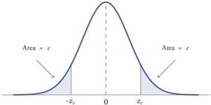
Figure 1. showing a 2-tail test for non-directional hypothesis for z for area C is the critical rejection region.

When a research hypothesis predicts a direction for the effect, it is called a directional hypothesis . To test the significance of a directional hypothesis, we have to consider the possibility that the sample could be extreme at one-tail of the comparison distribution. We call this a one-tailed test .

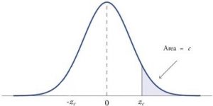
Figure 2. showing a 1-tail test for a directional hypothesis (predicting an increase) for z for area C is the critical rejection region.

Determining Cutoff Scores with Two-Tailed Tests

Typically we specify an α level before analyzing the data. If the data analysis results in a probability value below the α level, then the null hypothesis is rejected; if it is not, then the null hypothesis is not rejected. In other words, if our data produce values that meet or exceed this threshold, then we have sufficient evidence to reject the null hypothesis ; if not, we fail to reject the null (we never “accept” the null). According to this perspective, if a result is significant, then it does not matter how significant it is. Moreover, if it is not significant, then it does not matter how close to being significant it is. Therefore, if the 0.05 level is being used, then probability values of 0.049 and 0.001 are treated identically. Similarly, probability values of 0.06 and 0.34 are treated identically. Note we will discuss ways to address effect size (which is related to this challenge of NHST).

When setting the probability value, there is a special complication in a two-tailed test. We have to divide the significance percentage between the two tails. For example, with a 5% significance level, we reject the null hypothesis only if the sample is so extreme that it is in either the top 2.5% or the bottom 2.5% of the comparison distribution. This keeps the overall level of significance at a total of 5%. A one-tailed test does have such an extreme value but with a one-tailed test only one side of the distribution is considered.

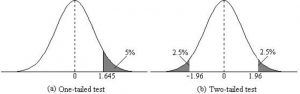
Figure 3. Critical value differences in one and two-tail tests. Photo Credit

Let’s re view th e set critical values for Z.

We discussed z-scores and probability in chapter 8.  If we revisit the z-score for 5% and 1%, we can identify the critical regions for the critical rejection areas from the unit standard normal table.

• A two-tailed test at the 5% level has a critical boundary Z score of +1.96 and -1.96
• A one-tailed test at the 5% level has a critical boundary Z score of +1.64 or -1.64
• A two-tailed test at the 1% level has a critical boundary Z score of +2.58 and -2.58
• A one-tailed test at the 1% level has a critical boundary Z score of +2.33 or -2.33.

Review: Critical values, p-values, and significance level

There are two criteria we use to assess whether our data meet the thresholds established by our chosen significance level, and they both have to do with our discussions of probability and distributions. Recall that probability refers to the likelihood of an event, given some situation or set of conditions. In hypothesis testing, that situation is the assumption that the null hypothesis value is the correct value, or that there is no effec t. The value laid out in H 0 is our condition under which we interpret our results. To reject this assumption, and thereby reject the null hypothesis, we need results that would be very unlikely if the null was true.

Now recall that values of z which fall in the tails of the standard normal distribution represent unlikely values. That is, the proportion of the area under the curve as or more extreme than z is very small as we get into the tails of the distribution. Our significance level corresponds to the area under the tail that is exactly equal to α: if we use our normal criterion of α = .05, then 5% of the area under the curve becomes what we call the rejection region (also called the critical region) of the distribution. This is illustrated in Figure 4.

Figure 4: The rejection region for a one-tailed test

The shaded rejection region takes us 5% of the area under the curve. Any result which falls in that region is sufficient evidence to reject the null hypothesis.

The rejection region is bounded by a specific z-value, as is any area under the curve. In hypothesis testing, the value corresponding to a specific rejection region is called the critical value, z crit (“z-crit”) or z* (hence the other name “critical region”). Finding the critical value works exactly the same as finding the z-score corresponding to any area under the curve like we did in Unit 1. If we go to the normal table, we will find that the z-score corresponding to 5% of the area under the curve is equal to 1.645 (z = 1.64 corresponds to 0.0405 and z = 1.65 corresponds to 0.0495, so .05 is exactly in between them) if we go to the right and -1.645 if we go to the left. The direction must be determined by your alternative hypothesis, and drawing then shading the distribution is helpful for keeping directionality straight.

Suppose, however, that we want to do a non-directional test. We need to put the critical region in both tails, but we don’t want to increase the overall size of the rejection region (for reasons we will see later). To do this, we simply split it in half so that an equal proportion of the area under the curve falls in each tail’s rejection region. For α = .05, this means 2.5% of the area is in each tail, which, based on the z-table, corresponds to critical values of z* = ±1.96. This is shown in Figure 5.

Figure 5: Two-tailed rejection region

Thus, any z-score falling outside ±1.96 (greater than 1.96 in absolute value) falls in the rejection region. When we use z-scores in this way, the obtained value of z (sometimes called z-obtained) is something known as a test statistic, which is simply an inferential statistic used to test a null hypothesis.

Calculate the test statistic: Z

Now that we understand setting up the hypothesis and determining the outcome, let’s examine hypothesis testing with z!  The next step is to carry out the study and get the actual results for our sample. Central to hypothesis test is comparison of the population and sample means. To make our calculation and determine where the sample is in the hypothesized distribution we calculate the Z for the sample data.

Make a decision

To decide whether to reject the null hypothesis, we compare our sample’s Z score to the Z score that marks our critical boundary. If our sample Z score falls inside the rejection region of the comparison distribution (is greater than the z-score critical boundary) we reject the null hypothesis.

The formula for our z- statistic has not changed:

To formally test our hypothesis, we compare our obtained z-statistic to our critical z-value. If z obt > z crit , that means it falls in the rejection region (to see why, draw a line for z = 2.5 on Figure 1 or Figure 2) and so we reject H 0 . If z obt < z crit , we fail to reject. Remember that as z gets larger, the corresponding area under the curve beyond z gets smaller. Thus, the proportion, or p-value, will be smaller than the area for α, and if the area is smaller, the probability gets smaller. Specifically, the probability of obtaining that result, or a more extreme result, under the condition that the null hypothesis is true gets smaller.

Conversely, if we fail to reject, we know that the proportion will be larger than α because the z-statistic will not be as far into the tail. This is illustrated for a one- tailed test in Figure 6.

Figure 6. Relation between α, z obt , and p

When the null hypothesis is rejected, the effect is said to be statistically significant . Do not confuse statistical significance with practical significance. A small effect can be highly significant if the sample size is large enough.

Why does the word “significant” in the phrase “statistically significant” mean something so different from other uses of the word? Interestingly, this is because the meaning of “significant” in everyday language has changed. It turns out that when the procedures for hypothesis testing were developed, something was “significant” if it signified something. Thus, finding that an effect is statistically significant signifies that the effect is real and not due to chance. Over the years, the meaning of “significant” changed, leading to the potential misinterpretation.

Review: Steps of the Hypothesis Testing Process

The process of testing hypotheses follows a simple four-step procedure. This process will be what we use for the remained of the textbook and course, and though the hypothesis and statistics we use will change, this process will not.

Step 1: State the Hypotheses

Your hypotheses are the first thing you need to lay out. Otherwise, there is nothing to test! You have to state the null hypothesis (which is what we test) and the alternative hypothesis (which is what we expect). These should be stated mathematically as they were presented above AND in words, explaining in normal English what each one means in terms of the research question.

Step 2: Find the Critical Values

Next, we formally lay out the criteria we will use to test our hypotheses. There are two pieces of information that inform our critical values: α, which determines how much of the area under the curve composes our rejection region, and the directionality of the test, which determines where the region will be.

Step 3: Compute the Test Statistic

Once we have our hypotheses and the standards we use to test them, we can collect data and calculate our test statistic, in this case z . This step is where the vast majority of differences in future chapters will arise: different tests used for different data are calculated in different ways, but the way we use and interpret them remains the same.

Step 4: Make the Decision

Finally, once we have our obtained test statistic, we can compare it to our critical value and decide whether we should reject or fail to reject the null hypothesis. When we do this, we must interpret the decision in relation to our research question, stating what we concluded, what we based our conclusion on, and the specific statistics we obtained.

Example: Movie Popcorn

Let’s see how hypothesis testing works in action by working through an example. Say that a movie theater owner likes to keep a very close eye on how much popcorn goes into each bag sold, so he knows that the average bag has 8 cups of popcorn and that this varies a little bit, about half a cup. That is, the known population mean is μ = 8.00 and the known population standard deviation is σ =0.50. The owner wants to make sure that the newest employee is filling bags correctly, so over the course of a week he randomly assesses 25 bags filled by the employee to test for a difference (n = 25). He doesn’t want bags overfilled or under filled, so he looks for differences in both directions. This scenario has all of the information we need to begin our hypothesis testing procedure.

Our manager is looking for a difference in the mean cups of popcorn bags compared to the population mean of 8. We will need both a null and an alternative hypothesis written both mathematically and in words. We’ll always start with the null hypothesis:

H 0 : There is no difference in the cups of popcorn bags from this employee H 0 : μ = 8.00

Notice that we phrase the hypothesis in terms of the population parameter μ, which in this case would be the true average cups of bags filled by the new employee.

Our assumption of no difference, the null hypothesis, is that this mean is exactly

the same as the known population mean value we want it to match, 8.00. Now let’s do the alternative:

H A : There is a difference in the cups of popcorn bags from this employee H A : μ ≠ 8.00

In this case, we don’t know if the bags will be too full or not full enough, so we do a two-tailed alternative hypothesis that there is a difference.

Our critical values are based on two things: the directionality of the test and the level of significance. We decided in step 1 that a two-tailed test is the appropriate directionality. We were given no information about the level of significance, so we assume that α = 0.05 is what we will use. As stated earlier in the chapter, the critical values for a two-tailed z-test at α = 0.05 are z* = ±1.96. This will be the criteria we use to test our hypothesis. We can now draw out our distribution so we can visualize the rejection region and make sure it makes sense

Figure 7: Rejection region for z* = ±1.96

Step 3: Calculate the Test Statistic

Now we come to our formal calculations. Let’s say that the manager collects data and finds that the average cups of this employee’s popcorn bags is ̅X = 7.75 cups. We can now plug this value, along with the values presented in the original problem, into our equation for z:

So our test statistic is z = -2.50, which we can draw onto our rejection region distribution:

Figure 8: Test statistic location

Looking at Figure 5, we can see that our obtained z-statistic falls in the rejection region. We can also directly compare it to our critical value: in terms of absolute value, -2.50 > -1.96, so we reject the null hypothesis. We can now write our conclusion:

When we write our conclusion, we write out the words to communicate what it actually means, but we also include the average sample size we calculated (the exact location doesn’t matter, just somewhere that flows naturally and makes sense) and the z-statistic and p-value. We don’t know the exact p-value, but we do know that because we rejected the null, it must be less than α.

Effect Size

When we reject the null hypothesis, we are stating that the difference we found was statistically significant, but we have mentioned several times that this tells us nothing about practical significance. To get an idea of the actual size of what we found, we can compute a new statistic called an effect size. Effect sizes give us an idea of how large, important, or meaningful a statistically significant effect is.

For mean differences like we calculated here, our effect size is Cohen’s d :

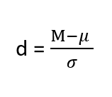
Effect sizes are incredibly useful and provide important information and clarification that overcomes some of the weakness of hypothesis testing. Whenever you find a significant result, you should always calculate an effect size

Table 1. Interpretation of Cohen’s d

Example: Office Temperature

Let’s do another example to solidify our understanding. Let’s say that the office building you work in is supposed to be kept at 74 degree Fahrenheit but is allowed

to vary by 1 degree in either direction. You suspect that, as a cost saving measure, the temperature was secretly set higher. You set up a formal way to test your hypothesis.

You start by laying out the null hypothesis:

H 0 : There is no difference in the average building temperature H 0 : μ = 74

Next you state the alternative hypothesis. You have reason to suspect a specific direction of change, so you make a one-tailed test:

H A : The average building temperature is higher than claimed H A : μ > 74

Now that you have everything set up, you spend one week collecting temperature data:

You calculate the average of these scores to be 𝑋̅ = 76.6 degrees. You use this to calculate the test statistic, using μ = 74 (the supposed average temperature), σ = 1.00 (how much the temperature should vary), and n = 5 (how many data points you collected):

z = 76.60 − 74.00 = 2.60    = 5.78

          1.00/√5            0.45

This value falls so far into the tail that it cannot even be plotted on the distribution!

Figure 7: Obtained z-statistic

You compare your obtained z-statistic, z = 5.77, to the critical value, z* = 1.645, and find that z > z*. Therefore you reject the null hypothesis, concluding: Based on 5 observations, the average temperature (𝑋̅ = 76.6 degrees) is statistically significantly higher than it is supposed to be, z = 5.77, p < .05.

d = (76.60-74.00)/ 1= 2.60

The effect size you calculate is definitely large, meaning someone has some explaining to do!

Example: Different Significance Level

First, let’s take a look at an example phrased in generic terms, rather than in the context of a specific research question, to see the individual pieces one more time. This time, however, we will use a stricter significance level, α = 0.01, to test the hypothesis.

We will use 60 as an arbitrary null hypothesis value: H 0 : The average score does not differ from the population H 0 : μ = 50

We will assume a two-tailed test: H A : The average score does differ H A : μ ≠ 50

We have seen the critical values for z-tests at α = 0.05 levels of significance several times. To find the values for α = 0.01, we will go to the standard normal table and find the z-score cutting of 0.005 (0.01 divided by 2 for a two-tailed test) of the area in the tail, which is z crit * = ±2.575. Notice that this cutoff is much higher than it was for α = 0.05. This is because we need much less of the area in the tail, so we need to go very far out to find the cutoff. As a result, this will require a much larger effect or much larger sample size in order to reject the null hypothesis.

We can now calculate our test statistic.  The average of 10 scores is M = 60.40 with a µ = 60. We will use σ = 10 as our known population standard deviation. From this information, we calculate our z-statistic as:

Our obtained z-statistic, z = 0.13, is very small. It is much less than our critical value of 2.575. Thus, this time, we fail to reject the null hypothesis. Our conclusion would look something like:

Notice two things about the end of the conclusion. First, we wrote that p is greater than instead of p is less than, like we did in the previous two examples. This is because we failed to reject the null hypothesis. We don’t know exactly what the p- value is, but we know it must be larger than the α level we used to test our hypothesis. Second, we used 0.01 instead of the usual 0.05, because this time we tested at a different level. The number you compare to the p-value should always be the significance level you test at. Because we did not detect a statistically significant effect, we do not need to calculate an effect size. Note: some statisticians will suggest to always calculate effects size as a possibility of Type II error. Although insignificant, calculating d = (60.4-60)/10 = .04 which suggests no effect (and not a possibility of Type II error).

Review Considerations in Hypothesis Testing

Errors in hypothesis testing.

Keep in mind that rejecting the null hypothesis is not an all-or-nothing decision. The Type I error rate is affected by the α level: the lower the α level the lower the Type I error rate. It might seem that α is the probability of a Type I error. However, this is not correct. Instead, α is the probability of a Type I error given that the null hypothesis is true. If the null hypothesis is false, then it is impossible to make a Type I error. The second type of error that can be made in significance testing is failing to reject a false null hypothesis. This kind of error is called a Type II error.

Statistical Power

The statistical power of a research design is the probability of rejecting the null hypothesis given the sample size and expected relationship strength. Statistical power is the complement of the probability of committing a Type II error. Clearly, researchers should be interested in the power of their research designs if they want to avoid making Type II errors. In particular, they should make sure their research design has adequate power before collecting data. A common guideline is that a power of .80 is adequate. This means that there is an 80% chance of rejecting the null hypothesis for the expected relationship strength.

Given that statistical power depends primarily on relationship strength and sample size, there are essentially two steps you can take to increase statistical power: increase the strength of the relationship or increase the sample size. Increasing the strength of the relationship can sometimes be accomplished by using a stronger manipulation or by more carefully controlling extraneous variables to reduce the amount of noise in the data (e.g., by using a within-subjects design rather than a between-subjects design). The usual strategy, however, is to increase the sample size. For any expected relationship strength, there will always be some sample large enough to achieve adequate power.

Inferential statistics uses data from a sample of individuals to reach conclusions about the whole population. The degree to which our inferences are valid depends upon how we selected the sample (sampling technique) and the characteristics (parameters) of population data. Statistical analyses assume that sample(s) and population(s) meet certain conditions called statistical assumptions.

It is easy to check assumptions when using statistical software and it is important as a researcher to check for violations; if violations of statistical assumptions are not appropriately addressed then results may be interpreted incorrectly.

Learning Objectives

Having read the chapter, students should be able to:

• Conduct a hypothesis test using a z-score statistics, locating critical region, and make a statistical decision including.
• Explain the purpose of measuring effect size and power, and be able to compute Cohen’s d.

Exercises – Ch. 10

• List the main steps for hypothesis testing with the z-statistic. When and why do you calculate an effect size?
• z = 1.99, two-tailed test at α = 0.05
• z = 1.99, two-tailed test at α = 0.01
• z = 1.99, one-tailed test at α = 0.05
• You are part of a trivia team and have tracked your team’s performance since you started playing, so you know that your scores are normally distributed with μ = 78 and σ = 12. Recently, a new person joined the team, and you think the scores have gotten better. Use hypothesis testing to see if the average score has improved based on the following 8 weeks’ worth of score data: 82, 74, 62, 68, 79, 94, 90, 81, 80.
• A study examines self-esteem and depression in teenagers.  A sample of 25 teens with a low self-esteem are given the Beck Depression Inventory.  The average score for the group is 20.9.  For the general population, the average score is 18.3 with σ = 12.  Use a two-tail test with α = 0.05 to examine whether teenagers with low self-esteem show significant differences in depression.
• You get hired as a server at a local restaurant, and the manager tells you that servers’ tips are $42 on average but vary about $12 (μ = 42, σ = 12). You decide to track your tips to see if you make a different amount, but because this is your first job as a server, you don’t know if you will make more or less in tips. After working 16 shifts, you find that your average nightly amount is $44.50 from tips. Test for a difference between this value and the population mean at the α = 0.05 level of significance.

Answers to Odd- Numbered Exercises – Ch. 10

1. List hypotheses. Determine critical region. Calculate z.  Compare z to critical region. Draw Conclusion.  We calculate an effect size when we find a statistically significant result to see if our result is practically meaningful or important

5. Step 1: H 0 : μ = 42 “My average tips does not differ from other servers”, H A : μ ≠ 42 “My average tips do differ from others”

Introduction to Statistics for Psychology Copyright © 2021 by Alisa Beyer is licensed under a Creative Commons Attribution-NonCommercial-ShareAlike 4.0 International License , except where otherwise noted.

Share This Book

Critical Z-Values: Gatekeepers in Hypothesis Testing

The world of statistics is full of tools, techniques, and terminologies that help us navigate the vast seas of data and draw meaningful conclusions. Among the plethora of statistical terms, ‘critical Z-values’ stands out, especially when venturing into the domain of hypothesis testing. To comprehend the importance and application of critical Z-values, let’s dive deeper into its essence and workings.

Z-Values: A Brief Refresher

At its foundation, a Z-value, or Z-score, indicates how many standard deviations a data point is away from the mean in a given dataset. This score can be both positive and negative, denoting values above or below the mean, respectively.

Discover how to calculate the z-score

What Are Critical Z-Values?

Critical Z-values, often termed critical values, are threshold values set on a standard normal distribution curve. These values, usually one on the left (negative) and one on the right (positive), effectively create a boundary or region. When testing hypotheses, if your test statistic falls within this region, you would reject the null hypothesis in favor of the alternative hypothesis.

The selection of these critical values is directly linked to the significance level (often denoted as α) that the researcher or analyst has chosen. Commonly used significance levels include 0.05, 0.01, and 0.10.

The Mechanics of Critical Z-Values

To understand this concept better, let’s take the commonly used significance level of 0.05. If you’re conducting a two-tailed test (which means you’re considering extreme values on both ends of the distribution), you’d split this α into two, placing 0.025 in each tail. Using a Z-table or statistical software, you’d then identify the Z-values that correspond to these tail areas. For a significance level of 0.05, the critical Z-values are typically -1.96 and +1.96.

Critical Z-Values in Hypothesis Testing

Hypothesis testing is a methodological process where statisticians make an initial assumption (the null hypothesis) and test the validity of this assumption based on sample data.

The process typically follows these steps:

• State the Hypotheses: Formulate the null (Ho) and alternative hypotheses (Ha).
• Choose the Significance Level (α): Decide the threshold for rejecting the null hypothesis.
• Select the Test and Find the Critical Value(s): For a Z-test, this would be the critical Z-value.
• Compute the Test Statistic: Calculate the Z-score for your sample data.
• Make a Decision: If your test statistic falls within the critical region (beyond the critical Z-values), you’d reject the null hypothesis.

Examples and Applications

Example 1: Imagine a shoe manufacturer claims their shoes last an average of 365 days before showing significant wear. A competitor believes these shoes wear out faster and conducts a study with a sample of shoes. Using a significance level of 0.05 for a two-tailed test, the critical Z-values are -1.96 and +1.96. If the Z-score calculated from the sample data is -2.1 (indicating the shoes wore out faster than claimed), the null hypothesis would be rejected since -2.1 falls outside the critical values.

Example 2: A beverage company claims its juice box contains 250 ml of juice. A consumer group, suspecting the company overstates the quantity, tests a sample. Using a one-tailed test at α = 0.05 (because they only care if the juice box contains less than claimed), the critical Z-value for this test would be -1.645. If their sample calculation results in a Z-score of -1.8, the null hypothesis would be rejected, suggesting the juice boxes contain less than the stated amount.

Why Are Critical Z-Values Important?

Critical Z-values serve as gatekeepers. They provide the boundary beyond which the observed data is considered rare or unusual under the assumption that the null hypothesis is true. By setting these boundaries, statisticians have a clear framework to determine whether to reject the null hypothesis or fail to reject it.

Find out everything you need to know about standard deviation

Critical Z-values, while just numbers on the surface, are pivotal in hypothesis testing, guiding decisions and providing clarity. They act as the yardstick against which observed data is measured, helping determine the validity of initial assumptions. In a world drowning in data, tools like critical Z-values help sieve through the noise, enabling researchers, analysts, and professionals to draw significant, actionable insights. As the backbone of hypothesis testing, understanding and applying critical Z-values is indispensable for anyone seeking to make informed decisions based on data.

Leave a Comment Cancel reply

Save my name, email, and website in this browser for the next time I comment.

Z-Test for Statistical Hypothesis Testing Explained

The Z-test is a statistical hypothesis test used to determine where the distribution of the test statistic we are measuring, like the mean , is part of the normal distribution .

There are multiple types of Z-tests, however, we’ll focus on the easiest and most well known one, the one sample mean test. This is used to determine if the difference between the mean of a sample and the mean of a population is statistically significant.

What Is a Z-Test?

A Z-test is a type of statistical hypothesis test where the test-statistic follows a normal distribution.  

The name Z-test comes from the Z-score of the normal distribution. This is a measure of how many standard deviations away a raw score or sample statistics is from the populations’ mean.

Z-tests are the most common statistical tests conducted in fields such as healthcare and data science . Therefore, it’s an essential concept to understand.

Requirements for a Z-Test

In order to conduct a Z-test, your statistics need to meet a few requirements, including:

• A Sample size that’s greater than 30. This is because we want to ensure our sample mean comes from a distribution that is normal. As stated by the c entral limit theorem , any distribution can be approximated as normally distributed if it contains more than 30 data points.
• The standard deviation and mean of the population is known .
• The sample data is collected/acquired randomly .

More on Data Science:   What Is Bootstrapping Statistics?

Z-Test Steps

There are four steps to complete a Z-test. Let’s examine each one.

4 Steps to a Z-Test

• State the null hypothesis.
• State the alternate hypothesis.
• Choose your critical value.
• Calculate your Z-test statistics. 

1. State the Null Hypothesis

The first step in a Z-test is to state the null hypothesis, H_0 . This what you believe to be true from the population, which could be the mean of the population, μ_0 :

2. State the Alternate Hypothesis

Next, state the alternate hypothesis, H_1 . This is what you observe from your sample. If the sample mean is different from the population’s mean, then we say the mean is not equal to μ_0:

3. Choose Your Critical Value

Then, choose your critical value, α , which determines whether you accept or reject the null hypothesis. Typically for a Z-test we would use a statistical significance of 5 percent which is z = +/- 1.96 standard deviations from the population’s mean in the normal distribution:

This critical value is based on confidence intervals.

4. Calculate Your Z-Test Statistic

Compute the Z-test Statistic using the sample mean, μ_1 , the population mean, μ_0 , the number of data points in the sample, n and the population’s standard deviation, σ :

If the test statistic is greater (or lower depending on the test we are conducting) than the critical value, then the alternate hypothesis is true because the sample’s mean is statistically significant enough from the population mean.

Another way to think about this is if the sample mean is so far away from the population mean, the alternate hypothesis has to be true or the sample is a complete anomaly.

More on Data Science: Basic Probability Theory and Statistics Terms to Know

Z-Test Example

Let’s go through an example to fully understand the one-sample mean Z-test.

A school says that its pupils are, on average, smarter than other schools. It takes a sample of 50 students whose average IQ measures to be 110. The population, or the rest of the schools, has an average IQ of 100 and standard deviation of 20. Is the school’s claim correct?

The null and alternate hypotheses are:

Where we are saying that our sample, the school, has a higher mean IQ than the population mean.

Now, this is what’s called a right-sided, one-tailed test as our sample mean is greater than the population’s mean. So, choosing a critical value of 5 percent, which equals a Z-score of 1.96 , we can only reject the null hypothesis if our Z-test statistic is greater than 1.96.

If the school claimed its students’ IQs were an average of 90, then we would use a left-tailed test, as shown in the figure above. We would then only reject the null hypothesis if our Z-test statistic is less than -1.96.

Computing our Z-test statistic, we see:

Therefore, we have sufficient evidence to reject the null hypothesis, and the school’s claim is right.

Hope you enjoyed this article on Z-tests. In this post, we only addressed the most simple case, the one-sample mean test. However, there are other types of tests, but they all follow the same process just with some small nuances.  

Built In’s expert contributor network publishes thoughtful, solutions-oriented stories written by innovative tech professionals. It is the tech industry’s definitive destination for sharing compelling, first-person accounts of problem-solving on the road to innovation.

Great Companies Need Great People. That's Where We Come In.

Hypothesis Testing for Means & Proportions

•   1  
• |   2  
• |   3  
• |   4  
• |   5  
• |   6  
• |   7  
• |   8  
• |   9  
• |   10  

Hypothesis Testing: Upper-, Lower, and Two Tailed Tests

Type i and type ii errors.

All Modules

Z score Table

t score Table

The procedure for hypothesis testing is based on the ideas described above. Specifically, we set up competing hypotheses, select a random sample from the population of interest and compute summary statistics. We then determine whether the sample data supports the null or alternative hypotheses. The procedure can be broken down into the following five steps.  

• Step 1. Set up hypotheses and select the level of significance α.

H 0 : Null hypothesis (no change, no difference);  

H 1 : Research hypothesis (investigator's belief); α =0.05

• Step 2. Select the appropriate test statistic.  

The test statistic is a single number that summarizes the sample information.   An example of a test statistic is the Z statistic computed as follows:

When the sample size is small, we will use t statistics (just as we did when constructing confidence intervals for small samples). As we present each scenario, alternative test statistics are provided along with conditions for their appropriate use.

• Step 3.  Set up decision rule.  

The decision rule is a statement that tells under what circumstances to reject the null hypothesis. The decision rule is based on specific values of the test statistic (e.g., reject H 0 if Z > 1.645). The decision rule for a specific test depends on 3 factors: the research or alternative hypothesis, the test statistic and the level of significance. Each is discussed below.

• The decision rule depends on whether an upper-tailed, lower-tailed, or two-tailed test is proposed. In an upper-tailed test the decision rule has investigators reject H 0 if the test statistic is larger than the critical value. In a lower-tailed test the decision rule has investigators reject H 0 if the test statistic is smaller than the critical value.  In a two-tailed test the decision rule has investigators reject H 0 if the test statistic is extreme, either larger than an upper critical value or smaller than a lower critical value.
• The exact form of the test statistic is also important in determining the decision rule. If the test statistic follows the standard normal distribution (Z), then the decision rule will be based on the standard normal distribution. If the test statistic follows the t distribution, then the decision rule will be based on the t distribution. The appropriate critical value will be selected from the t distribution again depending on the specific alternative hypothesis and the level of significance.  
• The third factor is the level of significance. The level of significance which is selected in Step 1 (e.g., α =0.05) dictates the critical value.   For example, in an upper tailed Z test, if α =0.05 then the critical value is Z=1.645.  

The following figures illustrate the rejection regions defined by the decision rule for upper-, lower- and two-tailed Z tests with α=0.05. Notice that the rejection regions are in the upper, lower and both tails of the curves, respectively. The decision rules are written below each figure.

Rejection Region for Lower-Tailed Z Test (H 1 : μ < μ 0 ) with α =0.05

The decision rule is: Reject H 0 if Z < 1.645.

Rejection Region for Two-Tailed Z Test (H 1 : μ ≠ μ 0 ) with α =0.05

The decision rule is: Reject H 0 if Z < -1.960 or if Z > 1.960.

The complete table of critical values of Z for upper, lower and two-tailed tests can be found in the table of Z values to the right in "Other Resources."

Critical values of t for upper, lower and two-tailed tests can be found in the table of t values in "Other Resources."

• Step 4. Compute the test statistic.  

Here we compute the test statistic by substituting the observed sample data into the test statistic identified in Step 2.

• Step 5. Conclusion.  

The final conclusion is made by comparing the test statistic (which is a summary of the information observed in the sample) to the decision rule. The final conclusion will be either to reject the null hypothesis (because the sample data are very unlikely if the null hypothesis is true) or not to reject the null hypothesis (because the sample data are not very unlikely).  

If the null hypothesis is rejected, then an exact significance level is computed to describe the likelihood of observing the sample data assuming that the null hypothesis is true. The exact level of significance is called the p-value and it will be less than the chosen level of significance if we reject H 0 .

Statistical computing packages provide exact p-values as part of their standard output for hypothesis tests. In fact, when using a statistical computing package, the steps outlined about can be abbreviated. The hypotheses (step 1) should always be set up in advance of any analysis and the significance criterion should also be determined (e.g., α =0.05). Statistical computing packages will produce the test statistic (usually reporting the test statistic as t) and a p-value. The investigator can then determine statistical significance using the following: If p < α then reject H 0 .  

• Step 1. Set up hypotheses and determine level of significance

H 0 : μ = 191 H 1 : μ > 191                 α =0.05

The research hypothesis is that weights have increased, and therefore an upper tailed test is used.

• Step 2. Select the appropriate test statistic.

Because the sample size is large (n > 30) the appropriate test statistic is

• Step 3. Set up decision rule.  

In this example, we are performing an upper tailed test (H 1 : μ> 191), with a Z test statistic and selected α =0.05.   Reject H 0 if Z > 1.645.

We now substitute the sample data into the formula for the test statistic identified in Step 2.  

We reject H 0 because 2.38 > 1.645. We have statistically significant evidence at a =0.05, to show that the mean weight in men in 2006 is more than 191 pounds. Because we rejected the null hypothesis, we now approximate the p-value which is the likelihood of observing the sample data if the null hypothesis is true. An alternative definition of the p-value is the smallest level of significance where we can still reject H 0 . In this example, we observed Z=2.38 and for α=0.05, the critical value was 1.645. Because 2.38 exceeded 1.645 we rejected H 0 . In our conclusion we reported a statistically significant increase in mean weight at a 5% level of significance. Using the table of critical values for upper tailed tests, we can approximate the p-value. If we select α=0.025, the critical value is 1.96, and we still reject H 0 because 2.38 > 1.960. If we select α=0.010 the critical value is 2.326, and we still reject H 0 because 2.38 > 2.326. However, if we select α=0.005, the critical value is 2.576, and we cannot reject H 0 because 2.38 < 2.576. Therefore, the smallest α where we still reject H 0 is 0.010. This is the p-value. A statistical computing package would produce a more precise p-value which would be in between 0.005 and 0.010. Here we are approximating the p-value and would report p < 0.010.                  

In all tests of hypothesis, there are two types of errors that can be committed. The first is called a Type I error and refers to the situation where we incorrectly reject H 0 when in fact it is true. This is also called a false positive result (as we incorrectly conclude that the research hypothesis is true when in fact it is not). When we run a test of hypothesis and decide to reject H 0 (e.g., because the test statistic exceeds the critical value in an upper tailed test) then either we make a correct decision because the research hypothesis is true or we commit a Type I error. The different conclusions are summarized in the table below. Note that we will never know whether the null hypothesis is really true or false (i.e., we will never know which row of the following table reflects reality).

Table - Conclusions in Test of Hypothesis

In the first step of the hypothesis test, we select a level of significance, α, and α= P(Type I error). Because we purposely select a small value for α, we control the probability of committing a Type I error. For example, if we select α=0.05, and our test tells us to reject H 0 , then there is a 5% probability that we commit a Type I error. Most investigators are very comfortable with this and are confident when rejecting H 0 that the research hypothesis is true (as it is the more likely scenario when we reject H 0 ).

When we run a test of hypothesis and decide not to reject H 0 (e.g., because the test statistic is below the critical value in an upper tailed test) then either we make a correct decision because the null hypothesis is true or we commit a Type II error. Beta (β) represents the probability of a Type II error and is defined as follows: β=P(Type II error) = P(Do not Reject H 0 | H 0 is false). Unfortunately, we cannot choose β to be small (e.g., 0.05) to control the probability of committing a Type II error because β depends on several factors including the sample size, α, and the research hypothesis. When we do not reject H 0 , it may be very likely that we are committing a Type II error (i.e., failing to reject H 0 when in fact it is false). Therefore, when tests are run and the null hypothesis is not rejected we often make a weak concluding statement allowing for the possibility that we might be committing a Type II error. If we do not reject H 0 , we conclude that we do not have significant evidence to show that H 1 is true. We do not conclude that H 0 is true.

 The most common reason for a Type II error is a small sample size.

return to top | previous page | next page

Content ©2017. All Rights Reserved. Date last modified: November 6, 2017. Wayne W. LaMorte, MD, PhD, MPH

Critical Value Approach in Hypothesis Testing

by Nathan Sebhastian

Posted on Jun 05, 2023

Reading time: 5 minutes

The critical value is the cut-off point to determine whether to accept or reject the null hypothesis for your sample distribution.

The critical value approach provides a standardized method for hypothesis testing, enabling you to make informed decisions based on the evidence obtained from sample data.

After calculating the test statistic using the sample data, you compare it to the critical value(s) corresponding to the chosen significance level ( α ).

The critical value(s) represent the boundary beyond which you reject the null hypothesis. You will have rejection regions and non-rejection region as follows:

Two-sided test

A two-sided hypothesis test has 2 rejection regions, so you need 2 critical values on each side. Because there are 2 rejection regions, you must split the significance level in half.

Each rejection region has a probability of α / 2 , making the total likelihood for both areas equal the significance level.

In this test, the null hypothesis H0 gets rejected when the test statistic is too small or too large.

Left-tailed test

The left-tailed test has 1 rejection region, and the null hypothesis only gets rejected when the test statistic is too small.

Right-tailed test

The right-tailed test is similar to the left-tailed test, only the null hypothesis gets rejected when the test statistic is too large.

Now that you understand the definition of critical values, let’s look at how to use critical values to construct a confidence interval.

Using Critical Values to Construct Confidence Intervals

Confidence Intervals use the same Critical values as the test you’re running.

If you’re running a z-test with a 95% confidence interval, then:

• For a two-sided test, The CVs are -1.96 and 1.96
• For a one-tailed test, the critical value is -1.65 (left) or 1.65 (right)

To calculate the upper and lower bounds of the confidence interval, you need to calculate the sample mean and then add or subtract the margin of error from it.

To get the Margin of Error, multiply the critical value by the standard error:

Let’s see an example. Suppose you are estimating the population mean with a 95% confidence level.

You have a sample mean of 50, a sample size of 100, and a standard deviation of 10. Using a z-table, the critical value for a 95% confidence level is approximately 1.96.

Calculate the standard error:

Determine the margin of error:

Compute the lower bound and upper bound:

The 95% confidence interval is (48.04, 51.96). This means that we are 95% confident that the true population mean falls within this interval.

Finding the Critical Value

The formula to find critical values depends on the specific distribution associated with the hypothesis test or confidence interval you’re using.

Here are the formulas for some commonly used distributions.

Standard Normal Distribution (Z-distribution):

The critical value for a given significance level ( α ) in the standard normal distribution is found using the cumulative distribution function (CDF) or a standard normal table.

z(α) represents the z-score corresponding to the desired significance level α .

Student’s t-Distribution (t-distribution):

The critical value for a given significance level (α) and degrees of freedom (df) in the t-distribution is found using the inverse cumulative distribution function (CDF) or a t-distribution table.

t(α, df) represents the t-score corresponding to the desired significance level α and degrees of freedom df .

Chi-Square Distribution (χ²-distribution):

The critical value for a given significance level (α) and degrees of freedom (df) in the chi-square distribution is found using the inverse cumulative distribution function (CDF) or a chi-square distribution table.

where χ²(α, df) represents the chi-square value corresponding to the desired significance level α and degrees of freedom df .

F-Distribution:

The critical value for a given significance level (α), degrees of freedom for the numerator (df₁), and degrees of freedom for the denominator (df₂) in the F-distribution is found using the inverse cumulative distribution function (CDF) or an F-distribution table.

F(α, df₁, df₂) represents the F-value corresponding to the desired significance level α , df₁ , and df₂ .

As you can see, the specific formula to find critical values depends on the distribution and the parameters associated with the problem at hand.

Usually, you don’t calculate the critical values manually as you can use statistical tables or statistical software to determine the critical values.

I will update this tutorial with statistical tables that you can use later.

The critical value is as a threshold where you make a decision based on the observed test statistic and its relation to the significance level.

It provides a predetermined point of reference to objectively evaluate the strength of the evidence against the null hypothesis and guide the acceptance or rejection of the hypothesis.

If the test statistic falls in the critical region (beyond the critical value), it means the observed data provide strong evidence against the null hypothesis.

In this case, you reject the null hypothesis in favor of the alternative hypothesis, indicating that there is sufficient evidence to support the claim or relationship stated in the alternative hypothesis.

On the other hand, if the test statistic falls in the non-critical region (within the critical value), it means the observed data do not provide enough evidence to reject the null hypothesis.

In this case, you fail to reject the null hypothesis, indicating that there is insufficient evidence to support the alternative hypothesis.

Take your skills to the next level ⚡️

I'm sending out an occasional email with the latest tutorials on programming, web development, and statistics. Drop your email in the box below and I'll send new stuff straight into your inbox!

Hello! This website is dedicated to help you learn tech and data science skills with its step-by-step, beginner-friendly tutorials. Learn statistics, JavaScript and other programming languages using clear examples written for people.

Learn more about this website

Connect with me on Twitter

Or LinkedIn

Type the keyword below and hit enter

Click to see all tutorials tagged with:

StatsCalculator.com

Z critical value calculator.

• Get Z Score
• P Value From Z Score
• t critical values

Other Stats Tools

• Descriptive Statistics
• Confidence Interval
• Correlation Coefficient
• Outlier Detection
• t-test - 1 Sample
• t-test - 2 Sample

alpha value

Tool Overview: Z Critical Value Calculator

Stuck trying to interpret the results of a statistical test - specifically finding the critical values for a standard normal distribution? You've come to the right place. Our free statistics package is intended as an alternative to Minitab and other paid software. This critical value calculator generates the critical values for a standard normal distribution for a given confidence level. The critical value is the point on a statistical distribution that represents an associated probability level. It generates critical values for both a left tailed test and a two-tailed test (splitting the alpha between the left and right side of the distribution). Simply enter the requested parameters (alpha level) into the calculator and hit calculate.

What Is a Critical Value and How Do You Use It?

A critical value is a concept from statistical testing. If we are performing hypothesis testing, we will reduce our proposition down to a single pair of choices, referred to as the null hypothesis and the alternative hypothesis . The null hypothesis denotes what we will believe to be correct if our sample data fails the statistical test. As a matter of form, it should usually reflect the default state for your process (eg. expected from normal operations). The alternative hypothesis represents an atypical outcome for the process, in which case we infer that something occured. We will then identify when and from where we shall draw a sample to assess which of these two alternatives is most likely to be correct. We will calculate a test statistic for the sample which we will compare to the expected distribution of the statistic to assess the relative probability of the hypothesis being correct. Bear in mind that this entire process exists in a probabilistic universe; we cannot opine on truth but only likelihood. We will identify the most appropriate distribution for comparing this sample (see below on when to use a standard normal vs. a t distribution). The critical value is the point in that distribution at which we must accept the alternative hypothesis as being more likely.

Note: This particular calculator is designed to find the critical value for the mean of a standard normal distribution. If your sample size is small (and you're still looking at the mean), you should use the t statistic sample distribution (we have a separate t score calculator for the t critical value). Both of these assume you're comparing the mean of the sample distribution to a fixed value. If you're trying to make inferences comparing the means of two populations (eg. both are "moving targets" vs. specified at a certain level, you're going to want to use the f statistic. (We're working on a calculator for the f critical value; you can find a table in the back of any statistics text book or here .)

In the case of the Z critical value all we need to calculate the critical value is the significance level (the alpha value) for the test. The alpha value reflects the probability of incorrectly rejecting the null hypothesis. The Z critical value is consistent for a given significance level regardless of sample size and numerator degrees. Common confidence levels for academic use are .05 (95% confidence), .025 (97.5%), and .01 (99%). That being said, a wise analyst compares the benefits of the required confidence level against the costs of achieving it (eg. don't always default to alpha .05 or .01).

How To Find Critical Values of Z

This calculator is intended to replace the use of a Z value table while providing access to a wider range of possible values for you to work with. In the offline version, you use a z score table (aka a z table) to look up the critical value for the test based on your desired level of alpha. Remember to adjust the alpha value based on wether you are doing a single-tailed test or two tailed test. In this case, we can simply split the value of alpha in two since the standard normal distsribution is symmetric about its axis. From there, finding the critical values for your test is a matter of looking up the appropriate row and column in the table. Our critical values calculator automates this process, so all you need to do is enter your alpha value and the tool will find the critical values for you.

When to Use Standard Normal (Z) vs. Student's T distribution

This calculator requires you to have sufficiently large sample that you are comfortable the values of the mean will converge on the standard normal distribution via the central limit theorem. This genreally requires you to have 30+ observations. If you are working with a smaller sample, you should consider using the version we set up to find critical values of a t-distribution . In any event, to run the hypothesis test you compare the observed value of the statistic with the t value from the t distribution table.

About this Website

This calculator is part of a larger collection of tools we've assembled as a free replacement to paid statistical packages. The other tools on this site include a descriptive statistics tool , confidence interval generators ( standard normal , proportions ), linear regression tools , and other tools for probability and statistics. Many calculators allow you to save and recycle your data in similar calculations, saving you time and frustration. Bookmark us and come back when you need a good source of free statistics tools.

Need more ideas? We also built this site too. We design word solver and analysis tools .

Other Tools: P Value From Z Score , P Value From T Score , Z critical value calculator , t critical value calculator

Understanding z-score and z-critical value in statistics: A comprehensive guide

8 months ago

In statistics, grasping various measures and their applications is essential for making informed decisions. Two often-used measures in statistical analysis are the z-score and z-critical value. We will delve into these topics section by section.

By the end of this article, you will clearly understand the differences between the Z score and Z value and know when to use each one for optimal statistical analysis.

What is a z-score?

A Z score , also known as a standard score, represents how many standard deviations a data point is from the mean of a set of data. It provides a way to compare the relative position of a value within a data set, allowing for standardized comparisons among different data sets or within the same data set.

The formula for calculating the Z score is:

Z = (X - μ) / σ

• Z is the z score
• X is the data point
• μ is the mean of the dataset
• σ is the standard deviation  

How to Find Z-Score?

Finding the Z-score is a standard procedure in statistics that allows you to determine how many standard deviations away a particular data point is from the mean of the dataset. The Z-score is beneficial in comparing data points across different distributions and understanding the relative positioning of data points within a distribution.

Follow these steps to find the z-score:

• Find the Mean (μ)

If you don't have it already, compute the mean of your dataset by adding up all the values and dividing by the number of values.

• Find the Standard Deviation (σ)

This is a measure of the amount of variation or dispersion in a set of values. You'll first find the variance by taking the average of the squared differences from the mean. Then, the standard deviation is the square root of the variance . There are formulas and tools available for computing this.

• Plug in the Values
• Subtract the mean from your specific data point (X−μ).
• Divide the result by the standard deviation.

Here's an example to learn how to calculate the Z-score.

We have a dataset of exam scores for a group of students. The mean score of the set is 75 and the standard deviation is 10. If a student scored 85 on the exam. Determine the Z score.

Solution:  

Step 1: Given values are:

Mean = μ = 75

Data point = X = 85

Standard deviation = σ = 10

Step 2: Take the formula and substitute the values in it.

Z score = Z = (X - μ) / σ

Putting the values:

Z = (85 - 75) / 10

This tells us that the Z score is 1 it is indicating that the student’s score is one standard deviation above the mean.

What is a z critical value?

A z critical value, often referred to as a critical value, is the number of standard deviations a data point needs to be from the mean to be considered statistically significant in a hypothesis test. It is closely associated with the concept of confidence levels and significance levels in hypothesis testing.

In simpler terms, the critical value is a cutoff point that helps determine whether or not the observed effect in the sample is statistically significant in the population.

How to find z critical value?

The Z critical value is found based on a prearranged significance level (often denoted as α) or confidence level.

The process to find the Z critical value can be described step by step:

For a Given Confidence Level:

Determine the total area for the two tails. If you have a 95% confidence level, the two tails combined would contain 5% (or 0.05) of the area under the standard normal curve because it is a two-tailed test. Each tail would then contain half of this, so 0.025 or 2.5%.

Using a standard normal (Z) table or calculator, find the Z value that corresponds to the cumulative probability of 1−0.025=0.9751−0.025=0.975 (for the right tail).

This Z value is your critical Z value. For a 95% confidence level, it would be approximately ±1.96.

For a Given Significance Level (α):

Decide if the test is one-tailed or two-tailed.

• For a two-tailed test: Divide α by 2. For α=0.05, this would give 0.025. Then, find the Z value corresponding to the cumulative probability of 1−0.025=0.9751−0.025=0.975 for the right tail. This Z value will be approximately ±1.96.
• For a right-tailed (upper) one-tailed test: Find the Z value corresponding to the cumulative probability of 1−α. For α=0.05, this would be 0.95. The Z value is approximately +1.645.
• For a left-tailed (lower) one-tailed test: Find the Z value corresponding to the cumulative probability of α. For α=0.05, this Z value is approximately -1.645.

The exact Z critical values might differ slightly depending on the source of the Z-table and Z critical value calculator.

Differences between z-score and z-critical value:

The Z-score and Z critical values both pertain to the standard normal distribution, but they serve different purposes and have different interpretations in statistics. Here's a breakdown of their differences:

When to Use Z Score & Z Critical Value?

Both the Z-score and the Z critical value are grounded in the standard normal distribution, but they are used in different contexts. Here's when to use each:

Z-score (Standard Score)

• Data Standardization: When you want to convert raw scores into standardized scores so they can be compared across different datasets or distributions. This is particularly useful when datasets have different means and standard deviations.
• Descriptive Analysis : To understand how unusual or typical a particular data point is within its distribution. A Z-score can tell you how many standard deviations a point is from the mean.
• Comparisons across Different Distributions : For instance, comparing SAT scores in Math and English. If you want to find out in which subject a student performed relatively better compared to peers, you'd use Z-scores.
• Detection of Outliers: A data point with a very high (or very low) Z-score might be considered an outlier.

Z Critical Value

Hypothesis testing:.

• Determining Rejection Regions: The Z critical value helps determine whether you should reject the null hypothesis. If your calculated Z-score exceeds the Z critical value (in absolute value), then you'd typically reject the null hypothesis.
• One-tailed vs. Two-tailed Tests : The side and the number of tails in your test will determine which Z critical values you use. For instance, a two-tailed test with a significance level of 0.05 will have critical values of -1.96 and +1.96.

Constructing Confidence Intervals:

When you want to estimate an interval for a population parameter based on sample data. For a 95% confidence interval for a normally distributed population (where the population standard deviation is known), you'd use the Z critical value of ±1.96 to construct the interval.

Determination of Sample Size:

When planning an experiment or survey and you want a certain confidence level and margin of error, the Z critical value is used to calculate the necessary sample size.

The Z-score and Z critical value are essential statistical measures that play distinct roles in data analysis. The Z-score measures the distance of a data point from the mean in terms of standard deviations, while the Z critical value sets threshold values used for hypothesis testing.

Understanding the differences between these two measures is crucial for making accurate statistical inferences and informed decisions across various fields. So, whether you’re analyzing exam scores or conducting complex research, remember to use the appropriate measure, as it can significantly impact the outcome of your analysis.

Question 1:

Is the Z value always positive?

Yes, the Z value is always non-negative, as it represents the number of standard deviations a given value is from the mean.

Question 2:

What is the significance of the Z value in hypothesis testing?

Answer: 

The Z value, also known as the critical value, helps in hypothesis testing by determining the probability of observing a value within a specific range from the mean. It assists in making decisions about accepting or rejecting the null hypothesis.

Question 3:

Can the Z score be negative?

Yes. The Z score can be negative if the data point is below the mean of the dataset.

Question 4:

What is the purpose of using the Z score in statistics?

The Z score is used to standardize data and determine how far a data point is from the mean of a dataset. It helps in comparing different data points on a common scale and makes it easier to analyze and interpret the data.

Recent Blogs

F Critical Value: Definition, formula, and Calculations

T Critical Value: Definition, Formula, Interpretation, and Examples

P-value: Definition, formula, interpretation, and use with examples

Criticalvaluecalculator.com is a free online service for students, researchers, and statisticians to find the critical values of t and z for right-tailed, left tailed, and two-tailed probability.

Information

• Privacy Policy
• Terms of Services

Critical Value Calculator

Use this calculator for critical values to easily convert a significance level to its corresponding Z value, T score, F-score, or Chi-square value. Outputs the critical region as well. The tool supports one-tailed and two-tailed significance tests / probability values.

Related calculators

• Using the critical value calculator
• What is a critical value?
• T critical value calculation
• Z critical value calculation
• F critical value calculation

    Using the critical value calculator

If you want to perform a statistical test of significance (a.k.a. significance test, statistical significance test), determining the value of the test statistic corresponding to the desired significance level is necessary. You need to know the desired error probability ( p-value threshold , common values are 0.05, 0.01, 0.001) corresponding to the significance level of the test. If you know the significance level in percentages, simply subtract it from 100%. For example, 95% significance results in a probability of 100%-95% = 5% = 0.05 .

Then you need to know the shape of the error distribution of the statistic of interest (not to be mistaken with the distribution of the underlying data!) . Our critical value calculator supports statistics which are either:

• Z -distributed (normally distributed, e.g. absolute difference of means)
• T -distributed (Student's T distribution, usually appropriate for small sample sizes, equivalent to the normal for sample sizes over 30)
• X 2 -distributed ( Chi square distribution, often used in goodness-of-fit tests, but also for tests of homogeneity or independence)
• F -distributed (Fisher-Snedecor distribution), usually used in analysis of variance (ANOVA)

Then, for distributions other than the normal one (Z), you need to know the degrees of freedom . For the F statistic there are two separate degrees of freedom - one for the numerator and one for the denominator.

Finally, to determine a critical region, one needs to know whether they are testing a point null versus a composite alternative (on both sides) or a composite null versus (covering one side of the distribution) a composite alternative (covering the other). Basically, it comes down to whether the inference is going to contain claims regarding the direction of the effect or not. Should one want to claim anything about the direction of the effect, the corresponding null hypothesis is direction as well (one-sided hypothesis).

Depending on the type of test - one-tailed or two-tailed, the calculator will output the critical value or values and the corresponding critical region. For one-sided tests it will output both possible regions, whereas for a two-sided test it will output the union of the two critical regions on the opposite sides of the distribution.

    What is a critical value?

A critical value (or values) is a point on the support of an error distribution which bounds a critical region from above or below. If the statistics falls below or above a critical value (depending on the type of hypothesis, but it has to fall inside the critical region) then a test is declared statistically significant at the corresponding significance level. For example, in a two-tailed Z test with critical values -1.96 and 1.96 (corresponding to 0.05 significance level) the critical regions are from -∞ to -1.96 and from 1.96 to +∞. Therefore, if the statistic falls below -1.96 or above 1.96, the null hypothesis test is statistically significant.

You can think of the critical value as a cutoff point beyond which events are considered rare enough to count as evidence against the specified null hypothesis. It is a value achieved by a distance function with probability equal to or greater than the significance level under the specified null hypothesis. In an error-probabilistic framework, a proper distance function based on a test statistic takes the generic form [1] :

X (read "X bar") is the arithmetic mean of the population baseline or the control, μ 0 is the observed mean / treatment group mean, while σ x is the standard error of the mean (SEM, or standard deviation of the error of the mean).

Here is how it looks in practice when the error is normally distributed (Z distribution) with a one-tailed null and alternative hypotheses and a significance level α set to 0.05:

And here is the same significance level when applied to a point null and a two-tailed alternative hypothesis:

The distance function would vary depending on the distribution of the error: Z, T, F, or Chi-square (X 2 ). The calculation of a particular critical value based on a supplied probability and error distribution is simply a matter of calculating the inverse cumulative probability density function (inverse CPDF) of the respective distribution. This can be a difficult task, most notably for the T distribution [2] .

    T critical value calculation

The T-distribution is often preferred in the social sciences, psychiatry, economics, and other sciences where low sample sizes are a common occurrence. Certain clinical studies also fall under this umbrella. This stems from the fact that for sample sizes over 30 it is practically equivalent to the normal distribution which is easier to work with. It was proposed by William Gosset, a.k.a. Student, in 1908 [3] , which is why it is also referred to as "Student's T distribution".

To find the critical t value, one needs to compute the inverse cumulative PDF of the T distribution. To do that, the significance level and the degrees of freedom need to be known. The degrees of freedom represent the number of values in the final calculation of a statistic that are free to vary whilst the statistic remains fixed at a certain value.

It should be noted that there is not, in fact, a single T-distribution, but there are infinitely many T-distributions, each with a different level of degrees of freedom. Below are some key values of the T-distribution with 1 degree of freedom, assuming a one-tailed T test is to be performed. These are often used as critical values to define rejection regions in hypothesis testing.

    Z critical value calculation

The Z-score is a statistic showing how many standard deviations away from the normal, usually the mean, a given observation is. It is often called just a standard score, z-value, normal score, and standardized variable. A Z critical value is just a particular cutoff in the error distribution of a normally-distributed statistic.

Z critical values are computed by using the inverse cumulative probability density function of the standard normal distribution with a mean (μ) of zero and standard deviation (σ) of one. Below are some commonly encountered probability values (significance levels) and their corresponding Z values for the critical region, assuming a one-tailed hypothesis .

The critical region defined by each of these would span from the Z value to plus infinity for the right-tailed case, and from minus infinity to minus the Z critical value in the left-tailed case. Our calculator for critical value will both find the critical z value(s) and output the corresponding critical regions for you.

Chi Square (Χ 2 ) critical value calculation

Chi square distributed errors are commonly encountered in goodness-of-fit tests and homogeneity tests, but also in tests for independence in contingency tables. Since the distribution is based on the squares of scores, it only contains positive values. Calculating the inverse cumulative PDF of the distribution is required in order to convert a desired probability (significance) to a chi square critical value.

Just like the T and F distributions, there is a different chi square distribution corresponding to different degrees of freedom. Hence, to calculate a Χ 2 critical value one needs to supply the degrees of freedom for the statistic of interest.

    F critical value calculation

F distributed errors are commonly encountered in analysis of variance (ANOVA), which is very common in the social sciences. The distribution, also referred to as the Fisher-Snedecor distribution, only contains positive values, similar to the Χ 2 one. Similar to the T distribution, there is no single F-distribution to speak of. A different F distribution is defined for each pair of degrees of freedom - one for the numerator and one for the denominator.

Calculating the inverse cumulative PDF of the F distribution specified by the two degrees of freedom is required in order to convert a desired probability (significance) to a critical value. There is no simple solution to find a critical value of f and while there are tables, using a calculator is the preferred approach nowadays.

    References

1 Mayo D.G., Spanos A. (2010) – "Error Statistics", in P. S. Bandyopadhyay & M. R. Forster (Eds.), Philosophy of Statistics, (7, 152–198). Handbook of the Philosophy of Science . The Netherlands: Elsevier.

2 Shaw T.W. (2006) – "Sampling Student's T distribution – use of the inverse cumulative distribution function", Journal of Computational Finance 9(4):37-73, DOI:10.21314/JCF.2006.150

3 "Student" [William Sealy Gosset] (1908) - "The probable error of a mean", Biometrika 6(1):1–25. DOI:10.1093/biomet/6.1.1

Cite this calculator & page

If you'd like to cite this online calculator resource and information as provided on the page, you can use the following citation: Georgiev G.Z., "Critical Value Calculator" , [online] Available at: https://www.gigacalculator.com/calculators/critical-value-calculator.php URL [Accessed Date: 16 May, 2024].

Our statistical calculators have been featured in scientific papers and articles published in high-profile science journals by:

The author of this tool

     Statistical calculators

• Critical Value

Calculate Critical Z Value

Enter a probability value between zero and one to calculate critical value. Critical values determine what probability a particular variable will have when a sampling distribution is normal or close to normal.

Probability (p): p = 1 - α/2.

Critical Value: Definition and Significance in the Real World

- Guide Authored by Corin B. Arenas , published on October 4, 2019

Ever wondered if election surveys are accurate? How about statistics on housing, health care, and testing scores?  

In this section, we’ll discuss how sample data is tested for accuracy. Read on to learn more about critical value, how it’s used in statistics, and its significance in social science research.

What is a Critical Value?

In testing statistics, a critical value is a factor that determines the margin of error in a distribution graph.

According to Statistics How To , a site headed by math educator Stephanie Glen, if the absolute value of a test statistic is greater than the critical value, then there is statistical significance that rejects an accepted hypothesis.

Critical values divide a distribution graph into sections which indicate ‘rejection regions.’ Basically, if a test value falls within a rejection region, it means an accepted hypothesis (referred to as a null hypothesis) must be rejected. And if the test value falls within the accepted range, the null hypothesis cannot be rejected.

Testing sample data involves validating research and surveys like voting habits, SAT scores, body fat percentage, blood pressure, and all sorts of population data.

Hypothesis Testing and the Distribution Curve

Hypothesis tests check if your data was taken from a sample population that adheres to a hypothesized probability distribution. It is characterized by a null hypothesis and an alternative hypothesis.

In hypothesis testing, a critical value is a point on a distribution graph that is analyzed alongside a test statistic to confirm if a null hypothesis —a commonly accepted fact in a study which researchers aim to disprove—should be rejected.

The value of a null hypothesis implies that no statistical significance exists in a set of given observations. It is assumed to be true unless statistical evidence from an alternative hypothesis invalidates it.  

How does this relate with distribution graphs? A normal distribution curve, which is a bell-shaped curve, is a theoretical representation of how often an experiment will yield a particular result.

Elements of Normal Distribution:

• Has a mean, median, or mode. A mean is the average of numbers in a group, a median is the middle number in a list of numbers, and a mode is a number that appears most often in a set of numbers.
• 50% of the values are less than the mean
• 50% of the values are greater than the mean

Majority of the data points in normal distribution are relatively similar. A perfectly normal distribution is characterized by its symmetry, meaning half of the data observations fall on either side of the middle of the graph. This implies that they occur within a range of values with fewer outliers on the high and low points of the graph.

Given these implications, critical values do not fall within the range of common data points. Which is why when a test statistic exceeds the critical value, a null hypothesis is forfeited.

Take note: Critical values may look for a two-tailed test or one-tailed test (right-tailed or left-tailed). Depending on the data, statisticians determine which test to perform first.

Finding the Critical Value

The standard equation for the probability of a critical value is:

p = 1 – α/2

Where p is the probability and alpha (α) represents the significance or confidence level. This establishes how far off a researcher will draw the line from the null hypothesis.

The alpha functions as the alternative hypothesis. It signifies the probability of rejecting the null hypothesis when it is true. For instance, if a researcher wants to establish a significance level of 0.05, it means there is a 5% chance of finding that a difference exists.

When the sampling distribution of a data set is normal or close to normal, the critical value can be determined as a z score or t score .

Z Score or T Score: Which Should You Use?

Typically, when a sample size is big (more than 40) using z or t statistics is fine. However, while both methods compute similar results, most beginner’s textbooks on statistics use the z score.

When a sample size is small and the standard deviation of a population is unknown, the t score is used. The t score is a probability distribution that allows statisticians to perform analyses on specific data sets using normal distribution. But take note: Small samples from populations that are not approximately normal should not use the t score.

What’s a standard deviation ? This measures how numbers are spread out in a set of values, showing the amount of variation. Low standard deviation means the numbers are close to the mean set, while a high standard deviation signifies numbers are dispersed at a wider range.

Calculating Z Score

The critical value of a z score can be used to determine the margin of error, as shown in the equations below:

• Margin of error = Critical value x Standard deviation of the statistic
• Margin of error = Critical value x Standard error of the statistic

The z score , also known as the standard normal probability score, signifies how many standard deviations a statistical element is from the mean. A z score table is used in hypothesis testing to check proportions and the difference between two means. Z tables indicate what percentage of the statistics is under the curve at any given point.

The basic formula for a z score sample is:

z = (X – μ) / σ

• X is the value of the element
• μ is the population mean
• σ is the standard deviation

Let’s solve an example. For instance, let’s say you have a test score of 85. If the test has a mean (μ) of 45 and a standard deviation (σ) of 23, what’s your z score? X = 85, μ = 45, σ = 23

z = (85 – 45) / 23 = 40 / 23 z = 1.7391

For this example, your score is 1.7391 standard deviations above the mean.

What do the z scores imply?

• If a score is greater than 0, the statistic sample is greater than the mean
• If the score is less than 0, the statistic sample is less than the mean
• If a score is equal to 1, it means the sample is 1 standard deviation greater than the mean, and so on
• If a score is equal to -1, it means the sample is 1 standard deviation less than the mean, and so on

For elements in a large set:

• Around 68% fall between -1 and 1
• Around 95% fall between -2 and 2
• Around 99% fall between -3 and 3

To give you an idea, here’s how spread out statistical elements would look like under a z score graph:

Calculating T Score

On the other hand, here’s the standard formula for the t score:

t = [ x – μ ] / [ s / sqrt( n ) ]

• x is the sample mean
• s is the sample’s standard deviation
• n is the sample size

Then, we account for the degrees of freedom (df) which is the sample size minus 1. df = n – 1

T distribution, also known as the student’s distribution, is associated with a unique cumulative probability. This signifies the chance of finding a sample mean that’s less than or equal to x, based on a random sample size n. Cumulative probability refers to the likelihood that a random variable would fall within a specific range. To express the t statistic with a cumulative probability of 1 – α, statisticians use t α .

Part of finding the t score is locating the degrees of freedom (df) using the t distribution table as a reference. For demonstration purposes, let’s say you have a small sample of 5 and you want to conduct a right-tailed test. Follow the steps below.

5 df, α = 0.05

• Take your sample size and subtract 1. 5 – 1 = 4. df = 4
• For this example, let’s say the alpha level is 5% (0.05).
• Look for the df in the t distribution table along with its corresponding alpha level. You’ll find the critical value where the column and row intersect.

*One-tail t distribution table referenced from How to Statistics. In this example, 5 df, α = 0.05, the critical value is 2.132.

Here’s another example using the t score formula.

A factory produces CFL light bulbs. The owner says that CFL bulbs from their factory lasts for 160 days. Quality specialists randomly chose 20 bulbs for testing, which lasted for an average of 150 days, with a standard deviation of 40 days. If the CFL bulbs really last for 160 days, what is the probability that 20 random CFL bulbs would have an average life that’s less than 150 days?

t = [ 150 – 160 ] / [ 40 / sqrt( 20 ) ] = -10 / [40 / 4.472135] = -10 / 8.94427 t = -1.118034

The degrees of freedom: df = 20 – 1, df = 19

Again, use the variables above to refer to a t distribution table, or use a t score calculator.

For this example, the critical value is 0.1387 . Thus, if the life of a CFL light bulb is 160 days, there is a 13.87% probability that the average CFL bulb for 20 randomly chosen bulbs would be less than or equal to 150 days.

If we were to plot the critical value and shade the rejection region in a graph, it would look like this:

If a test statistic is greater than this critical value, then the null hypothesis, which is ‘CFL light bulbs have a life of 160 days,’ should be rejected. That’s if tests show more than 13.87% of the sample light bulbs (20) have a lifespan of less than or equal 150 days.

Why is Determining Critical Value Important?

Researchers often work with a sample population, which is a small percentage when they gather statistics.

Working with sample populations does not guarantee that it reflects the actual population’s results. To test if the data is representative of the actual population, researchers conduct hypothesis testing which make use of critical values.

What are Real-World Uses for It?

Validating statistical knowledge is important in the study of a wide range of fields. This includes research in social sciences such as economics, psychology, sociology, political science, and anthropology.

For one, it keeps quality management in check. This includes product testing in companies and analyzing test scores in educational institutions.

Moreover, hypothesis testing is crucial for the scientific and medical community because it is imperative for the advancement of theories and ideas.

If you’ve come across research that studies behavior, then the study likely used hypothesis testing and sampling in populations. From the public’s voting behavior, to what type of houses people tend to buy, researchers conduct distribution tests.

Studies such as how male adolescents in certain states are prone to violence, or how children of obese parents are prone to becoming obese, are other examples that use critical values in distribution testing.

In the field of health care, topics like how often diseases like measles, diphtheria, or polio occur in an area is relevant for public safety. Testing would help communities know if there are certain health conditions rising at an alarming rate. This is especially relevant now in the age of anti-vaccine activists .

The Bottom Line

Finding critical values are important for testing statistical data. It’s one of the main factors in hypothesis testing, which can validate or disprove commonly accepted information.

Proper analysis and testing of statistics help guide the public, which corrects misleading or dated information.

Hypothesis testing is useful in a wide range of disciplines, such as medicine, sociology, political science, and quality management in companies.

About the Author

Corin is an ardent researcher and writer of financial topics—studying economic trends, how they affect populations, as well as how to help consumers make wiser financial decisions. Her other feature articles can be read on Inquirer.net and Manileno.com. She holds a Master’s degree in Creative Writing from the University of the Philippines, one of the top academic institutions in the world, and a Bachelor’s in Communication Arts from Miriam College.

How to Excel at Math Cartoon

• Trigonometry
• Percent Off
• Statistical Average
• Standard Deviation
• Correlation
• Probability
• Log/Antilog
• HEX & Binary
• Weight/Mass
• Temperature
• Current Time
• Time Duration
• Balance Equations

Play & Learn

Pin It on Pinterest

Statistics Made Easy

How to Find the Z Critical Value on a TI-84 Calculator

Whenever you conduct a hypothesis test, you will get a test statistic as a result. To determine if the results of the hypothesis test are statistically significant, you can compare the test statistic to a  Z critical value . If the absolute value of the test statistic is greater than the Z critical value, then the results of the test are statistically significant.

To find the Z critical value on a TI-84 calculator, we can use the following function:

invNorm(probability, μ, σ)

• probability: the significance level
• μ:  population mean
• σ: population standard deviation

You can access this function on a TI-84 calculator by pressing  2nd  and then pressing  vars . This will take you to a  DISTR  screen where you can then use  invNorm() :

This tutorial shares several examples of how to use the invNorm() function to find Z critical values on a TI-84 calculator.

Example 1: Z Critical Value for a Left-Tailed Test

Question:  Find the Z critical value for a left-tailed test with a significance level of 0.05.

Answer:  invNorm(.05, 0, 1) = -1.6449

Interpretation:  If the test statistic of the test is less than  -1.6449 , then the results of the test are statistically significant at α = 0.05.

Example 2: Z Critical Value for a Right-Tailed Test

Question:  Find the Z critical value for a right-tailed test with a significance level of 0.10.

Answer:  invT(1-.10, 0, 1) = 1.2816

Interpretation:  If the test statistic of the test is greater than 1.2816 , then the results of the test are statistically significant at α = 0.10.

Example 3: Z Critical Value for a Two-Tailed Test

Question:  Find the Z critical value for a two-tailed test with a significance level of 0.05.

Answer:  invNorm(.05/2, 0, 1) =  -1.96, 1.96

Interpretation: Since this is a two-tailed test, we actually have two critical values: -1.96 and  1.96 . If the test statistic of the test is less than -1.96  or greater than  1.96 , then the results of the test are statistically significant at α = 0.05.

Featured Posts

Hey there. My name is Zach Bobbitt. I have a Masters of Science degree in Applied Statistics and I’ve worked on machine learning algorithms for professional businesses in both healthcare and retail. I’m passionate about statistics, machine learning, and data visualization and I created Statology to be a resource for both students and teachers alike.  My goal with this site is to help you learn statistics through using simple terms, plenty of real-world examples, and helpful illustrations.

Leave a Reply Cancel reply

Your email address will not be published. Required fields are marked *

Join the Statology Community

Sign up to receive Statology's exclusive study resource: 100 practice problems with step-by-step solutions. Plus, get our latest insights, tutorials, and data analysis tips straight to your inbox!

By subscribing you accept Statology's Privacy Policy.

• school Campus Bookshelves
• menu_book Bookshelves
• perm_media Learning Objects
• login Login
• how_to_reg Request Instructor Account
• hub Instructor Commons

Margin Size

• Download Page (PDF)
• Download Full Book (PDF)
• Periodic Table
• Physics Constants
• Scientific Calculator
• Reference & Cite
• Tools expand_more
• Readability

selected template will load here

This action is not available.

8.5: Critical values, p-values, and significance level

• Last updated
• Save as PDF
• Page ID 14494

• Foster et al.
• University of Missouri-St. Louis, Rice University, & University of Houston, Downtown Campus via University of Missouri’s Affordable and Open Access Educational Resources Initiative

\( \newcommand{\vecs}[1]{\overset { \scriptstyle \rightharpoonup} {\mathbf{#1}} } \)

\( \newcommand{\vecd}[1]{\overset{-\!-\!\rightharpoonup}{\vphantom{a}\smash {#1}}} \)

\( \newcommand{\id}{\mathrm{id}}\) \( \newcommand{\Span}{\mathrm{span}}\)

( \newcommand{\kernel}{\mathrm{null}\,}\) \( \newcommand{\range}{\mathrm{range}\,}\)

\( \newcommand{\RealPart}{\mathrm{Re}}\) \( \newcommand{\ImaginaryPart}{\mathrm{Im}}\)

\( \newcommand{\Argument}{\mathrm{Arg}}\) \( \newcommand{\norm}[1]{\| #1 \|}\)

\( \newcommand{\inner}[2]{\langle #1, #2 \rangle}\)

\( \newcommand{\Span}{\mathrm{span}}\)

\( \newcommand{\id}{\mathrm{id}}\)

\( \newcommand{\kernel}{\mathrm{null}\,}\)

\( \newcommand{\range}{\mathrm{range}\,}\)

\( \newcommand{\RealPart}{\mathrm{Re}}\)

\( \newcommand{\ImaginaryPart}{\mathrm{Im}}\)

\( \newcommand{\Argument}{\mathrm{Arg}}\)

\( \newcommand{\norm}[1]{\| #1 \|}\)

\( \newcommand{\Span}{\mathrm{span}}\) \( \newcommand{\AA}{\unicode[.8,0]{x212B}}\)

\( \newcommand{\vectorA}[1]{\vec{#1}}      % arrow\)

\( \newcommand{\vectorAt}[1]{\vec{\text{#1}}}      % arrow\)

\( \newcommand{\vectorB}[1]{\overset { \scriptstyle \rightharpoonup} {\mathbf{#1}} } \)

\( \newcommand{\vectorC}[1]{\textbf{#1}} \)

\( \newcommand{\vectorD}[1]{\overrightarrow{#1}} \)

\( \newcommand{\vectorDt}[1]{\overrightarrow{\text{#1}}} \)

\( \newcommand{\vectE}[1]{\overset{-\!-\!\rightharpoonup}{\vphantom{a}\smash{\mathbf {#1}}}} \)

A low probability value casts doubt on the null hypothesis. How low must the probability value be in order to conclude that the null hypothesis is false? Although there is clearly no right or wrong answer to this question, it is conventional to conclude the null hypothesis is false if the probability value is less than 0.05. More conservative researchers conclude the null hypothesis is false only if the probability value is less than 0.01. When a researcher concludes that the null hypothesis is false, the researcher is said to have rejected the null hypothesis. The probability value below which the null hypothesis is rejected is called the \(α\) level or simply \(α\) (“alpha”). It is also called the significance level. If \(α\) is not explicitly specified, assume that \(α\) = 0.05.

The significance level is a threshold we set before collecting data in order to determine whether or not we should reject the null hypothesis. We set this value beforehand to avoid biasing ourselves by viewing our results and then determining what criteria we should use. If our data produce values that meet or exceed this threshold, then we have sufficient evidence to reject the null hypothesis; if not, we fail to reject the null (we never “accept” the null).

There are two criteria we use to assess whether our data meet the thresholds established by our chosen significance level, and they both have to do with our discussions of probability and distributions. Recall that probability refers to the likelihood of an event, given some situation or set of conditions. In hypothesis testing, that situation is the assumption that the null hypothesis value is the correct value, or that there is no effect. The value laid out in H 0  is our condition under which we interpret our results. To reject this assumption, and thereby reject the null hypothesis, we need results that would be very unlikely if the null was true. Now recall that values of z which fall in the tails of the standard normal distribution represent unlikely values. That is, the proportion of the area under the curve as or more extreme than \(z\) is very small as we get into the tails of the distribution. Our significance level corresponds to the area under the tail that is exactly equal to \(α\): if we use our normal criterion of \(α\) = .05, then 5% of the area under the curve becomes what we call the rejection region (also called the critical region) of the distribution. This is illustrated in Figure \(\PageIndex{1}\).

The shaded rejection region takes us 5% of the area under the curve. Any result which falls in that region is sufficient evidence to reject the null hypothesis.

The rejection region is bounded by a specific \(z\)-value, as is any area under the curve. In hypothesis testing, the value corresponding to a specific rejection region is called the critical value, \(z_{crit}\) (“\(z\)-crit”) or \(z*\) (hence the other name “critical region”). Finding the critical value works exactly the same as finding the z-score corresponding to any area under the curve like we did in Unit 1. If we go to the normal table, we will find that the z-score corresponding to 5% of the area under the curve is equal to 1.645 (\(z\) = 1.64 corresponds to 0.0505 and \(z\) = 1.65 corresponds to 0.0495, so .05 is exactly in between them) if we go to the right and -1.645 if we go to the left. The direction must be determined by your alternative hypothesis, and drawing then shading the distribution is helpful for keeping directionality straight.

Suppose, however, that we want to do a non-directional test. We need to put the critical region in both tails, but we don’t want to increase the overall size of the rejection region (for reasons we will see later). To do this, we simply split it in half so that an equal proportion of the area under the curve falls in each tail’s rejection region. For \(α\) = .05, this means 2.5% of the area is in each tail, which, based on the z-table, corresponds to critical values of \(z*\) = ±1.96. This is shown in Figure \(\PageIndex{2}\).

Thus, any \(z\)-score falling outside ±1.96 (greater than 1.96 in absolute value) falls in the rejection region. When we use \(z\)-scores in this way, the obtained value of \(z\) (sometimes called \(z\)-obtained) is something known as a test statistic, which is simply an inferential statistic used to test a null hypothesis. The formula for our \(z\)-statistic has not changed:

\[z=\dfrac{M-\mu}{\sigma / \sqrt{\mathrm{n}}} \]

To formally test our hypothesis, we compare our obtained \(z\)-statistic to our critical \(z\)-value. If \(\mathrm{Z}_{\mathrm{obt}}>\mathrm{Z}_{\mathrm{crit}}\), that means it falls in the rejection region (to see why, draw a line for \(z\) = 2.5 on Figure \(\PageIndex{1}\) or Figure \(\PageIndex{2}\)) and so we reject \(H_0\). If \(\mathrm{Z}_{\mathrm{obt}}<\mathrm{Z}_{\mathrm{crit}}\), we fail to reject. Remember that as \(z\) gets larger, the corresponding area under the curve beyond \(z\) gets smaller. Thus, the proportion, or \(p\)-value, will be smaller than the area for \(α\), and if the area is smaller, the probability gets smaller. Specifically, the probability of obtaining that result, or a more extreme result, under the condition that the null hypothesis is true gets smaller.

The \(z\)-statistic is very useful when we are doing our calculations by hand. However, when we use computer software, it will report to us a \(p\)-value, which is simply the proportion of the area under the curve in the tails beyond our obtained \(z\)-statistic. We can directly compare this \(p\)-value to \(α\) to test our null hypothesis: if \(p < α\), we reject \(H_0\), but if \(p > α\), we fail to reject. Note also that the reverse is always true: if we use critical values to test our hypothesis, we will always know if \(p\) is greater than or less than \(α\). If we reject, we know that \(p < α\) because the obtained \(z\)-statistic falls farther out into the tail than the critical \(z\)-value that corresponds to \(α\), so the proportion (\(p\)-value) for that \(z\)-statistic will be smaller. Conversely, if we fail to reject, we know that the proportion will be larger than \(α\) because the \(z\)-statistic will not be as far into the tail. This is illustrated for a one-tailed test in Figure \(\PageIndex{3}\).

When the null hypothesis is rejected, the effect is said to be statistically significant. For example, in the Physicians Reactions case study, the probability value is 0.0057. Therefore, the effect of obesity is statistically significant and the null hypothesis that obesity makes no difference is rejected. It is very important to keep in mind that statistical significance means only that the null hypothesis of exactly no effect is rejected; it does not mean that the effect is important, which is what “significant” usually means. When an effect is significant, you can have confidence the effect is not exactly zero. Finding that an effect is significant does not tell you about how large or important the effect is. Do not confuse statistical significance with practical significance. A small effect can be highly significant if the sample size is large enough. Why does the word “significant” in the phrase “statistically significant” mean something so different from other uses of the word? Interestingly, this is because the meaning of “significant” in everyday language has changed. It turns out that when the procedures for hypothesis testing were developed, something was “significant” if it signified something. Thus, finding that an effect is statistically significant signifies that the effect is real and not due to chance. Over the years, the meaning of “significant” changed, leading to the potential misinterpretation.

Contributors and Attributions

Foster et al.  (University of Missouri-St. Louis, Rice University, & University of Houston, Downtown Campus)

9.10: Testing a Claim about Population Proportion

Chapter 1: understanding statistics, chapter 2: summarizing and visualizing data, chapter 3: measure of central tendency, chapter 4: measures of variation, chapter 5: measures of relative standing, chapter 6: probability distributions, chapter 7: estimates, chapter 8: distributions, chapter 9: hypothesis testing, chapter 10: analysis of variance, chapter 11: correlation and regression, chapter 12: statistics in practice.

The JoVE video player is compatible with HTML5 and Adobe Flash. Older browsers that do not support HTML5 and the H.264 video codec will still use a Flash-based video player. We recommend downloading the newest version of Flash here, but we support all versions 10 and above.

In the natural populations of Trinidadian guppies, females select the males with orange coloration for mating.

To determine if guppy populations in an aquarium also show the same behavior, an experiment is conducted where 12 females are individually introduced to three orange males and three blue males simultaneously.

It is originally claimed that the females choose the orange males.

So, the null hypothesis would state that an equal number of females would show a preference for orange and blue males. The alternative hypothesis is that a higher number of females would prefer the orange males.

The experiment shows that ten out of twelve females preferred the orange males.

This ratio provides the sample proportion— 0.83—which is used to get the test statistic as follows.

It is observed that this test statistic falls within the critical region at a significance level of 0.05.

Also, the P -value from this z statistic is 0.011.

So, we may conclude that the aquarium population of guppies shows the same mating preference as observed in the natural population.

A complete procedure for testing a claim about a population proportion is provided here.

There are two methods of testing a claim about a population proportion: (1) Using the sample proportion from the data where a binomial distribution is approximated to the normal distribution and (2) Using the binomial probabilities calculated from the data.

The first method uses normal distribution as an approximation to the binomial distribution. The requirements are as follows: sample size is large enough, the probability of proportion p is close to 0.5, the np (product of sample size and proportion) is greater than 5, and the critical values can be calculated using the z distribution. It also requires the samples to be random and unbiased, and the nature of the data to be  binomial, i.e., there are only two possible outcomes (e.g., success or failure; selected or not selected, true or false, etc.). A proportion is binomial in nature. So, this method is well suitable for testing a claim using hypothesis testing for population proportion.

As a first step, the hypotheses (null and alternative hypotheses) are stated clearly and expressed symbolically. The proportion p used in hypotheses statements is the assumed proportion value, often 0.5. The proportion obtained from the data is the sample proportion. Both these values are crucial in calculating the z statistic.

The critical value can then be obtained from the z distribution utilizing  the normal approximation of the binomial distribution. The critical value can be positive or negative based on the hypothesis direction; accordingly, the hypothesis test is right-tailed, left-tailed, or two-tailed. The critical value is calculated at any desired confidence level, most commonly 95% or 99%.

The P -value is then directly calculated using the z statistic and the critical z value, and the hypothesis test is concluded. The z statistic can also be directly compared with the critical value to conclude the hypothesis test.

The second method of testing the claim about proportion does not require np > 5 as it uses the exact binomial distribution without normal approximation. This method does not calculate the critical value. Instead, it uses the probabilities of obtaining  x (the value of successes out of total trials, e.g., 60 successes out of 110 trials) in the n trials. It calculates the probabilities of x or fewer and x or greater and then leads to the  P -values. This second method of testing a claim about proportion is tedious to do manually and requires statistical software. Nonetheless, the inferences determined in both ways are equally accurate.

Get cutting-edge science videos from J o VE sent straight to your inbox every month.

mktb-description

We use cookies to enhance your experience on our website.

By continuing to use our website or clicking “Continue”, you are agreeing to accept our cookies.

Advertisement

Critical Values Robust to P-hacking

• Cite Icon Cite
• Open the PDF for in another window
• Permissions
• Article contents
• Figures & tables
• Supplementary Data
• Peer Review
• Search Site

Adam McCloskey , Pascal Michaillat; Critical Values Robust to P-hacking. The Review of Economics and Statistics 2024; doi: https://doi.org/10.1162/rest_a_01456

Download citation file:

• Ris (Zotero)
• Reference Manager

P-hacking is prevalent in reality but absent from classical hypothesis-testing theory. We therefore build a model of hypothesis testing that accounts for p-hacking. From the model, we derive critical values such that, if they are used to determine significance, and if p-hacking adjusts to the new significance standards, spurious significant results do not occur more often than intended. Because of p-hacking, such robust critical values are larger than classical critical values. In the model calibrated to medical science, the robust critical value is the classical critical value for the same test statistic but with one fifth of the significance level.

Article PDF first page preview

Supplementary data, email alerts, related articles, affiliations.

• Online ISSN 1530-9142
• Print ISSN 0034-6535

A product of The MIT Press

Mit press direct.

• About MIT Press Direct

Information

• Accessibility
• For Authors
• For Customers
• For Librarians
• Direct to Open
• Open Access
• Media Inquiries
• Rights and Permissions
• For Advertisers
• About the MIT Press
• The MIT Press Reader
• MIT Press Blog
• Seasonal Catalogs
• MIT Press Home
• Give to the MIT Press
• Direct Service Desk
• Terms of Use
• Privacy Statement
• Crossref Member
• COUNTER Member  
• The MIT Press colophon is registered in the U.S. Patent and Trademark Office

This Feature Is Available To Subscribers Only

Sign In or Create an Account