hypothesis testing non normal distribution

The Stats Geek

The t-test and robustness to non-normality

So, as constructed, the two-sample t-test assumes normality of the variable X in the two groups. On the face of it then, we would worry if, upon inspection of our data, say using histograms, we were to find that our data looked non-normal. In particular, we would worry that the t-test will not perform as it should – i.e. that if the null hypothesis is true, it will falsely reject the null 5% of the time (I’m assuming we are using the usual significance level).

What does this mean in practice? Provided our sample size isn’t too small, we shouldn’t be overly concerned if our data appear to violate the normal assumption. Also, for the same reasons, the 95% confidence interval for the difference in group means will have correct coverage, even when X is not normal (again, when the sample size is sufficiently large). Of course, for small samples, or highly skewed distributions, the above asymptotic result may not give a very good approximation, and so the type 1 error rate may deviate from the nominal 5% level.

Of course if X isn’t normally distributed, even if the type 1 error rate for the t-test assuming normality is close to 5%, the test will not be optimally powerful. That is, there will exist alternative tests of the null hypothesis which have greater power to detect alternative hypotheses.

For more on the large sample properties of hypothesis tests, robustness, and power, I would recommend looking at Chapter 3 of ’Elements of Large-Sample Theory’ by Lehmann. For more on the specific question of the t-test and robustness to non-normality, I’d recommend looking at this paper by Lumley and colleagues.

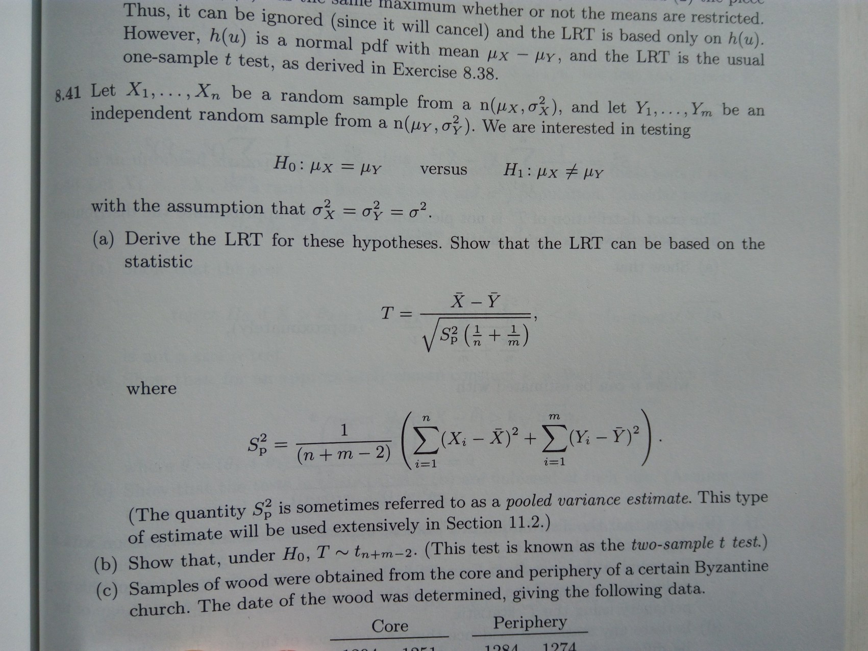
Addition – 1st May 2017 Below Teddy Warner queries in a comment whether the t-test ‘assumes’ normality of the individual observations. The following image is from the book Statistical Inference by Casella and Berger , and is provided just to illustrate the point that the t-test is, by its construction, based on assuming normality for the individual (population) values:

You may also be interested in:

• Wilcoxon-Mann-Whitney as an alternative to the t-test

9 thoughts on “The t-test and robustness to non-normality”

This website’s description and explanation of the “normality assumption” of t-tests (and by extension to ANOVA and MANOVA and regression) is simply incorrect. Parametric tests do not assume normality of sample scores nor even of the underlying population of scores from which samples scores are taken. Parametric tests assume that the sampling distribution of the statistic being test is normally distributed – that is, the sampling distribution of the mean or difference in means. Sampling distributions approach normality as sample size increases as shown by the Central Limit Theorem, and the consensus among experts is that with means that are based on sample sizes as small as 30 that the sampling distribution of means is so close to being a normal distribution, that the differences in probabilities in the tails of the normal and almost normal sampling distributions are not worth attention. Also, for any symmetrical distribution of scores, the sampling distribution will be normal. The normality assumption for Pearson correlation coefficients is also commonly misstated in MANY, if not most, online and textbook sources as requiring the variables being correlated to be normally distributed. X & Y variables do not require normal distributions, but only require that the sampling distribution of r (or t that is used to test the statistical significance of r) be normally distributed. In addition, many sources also misstate the normality assumption for regression and multiple regression as requiring that scores for predictor variables to be normally distributed. Regression only assumes that the residuals of the regression model being fit be normally distributed. Moreover, the assumption of normality for any statistical test is only relevant if one tests the null hypothesis because the sampling distribution has no effect on the parameter being estimated by the sample – that is, the sample mean and the sample correlation and the sample regression weights are the best unbiased estimates of their corresponding parameters, assuming there are no other “problems” with the data such as outliers, thus not affecting effect size estimates such as the values of r, R-square, b or Cohen’s d. Outliers usually should be trimmed, scores transformed or Winsorized because outliers can distort estimates of any parametric model. Of course, other assumptions may be important to consider beyond the normality assumption – such as heterscadasticity, independence of observations, and homogeneity of variances. But telling people that their data need to be normally distributed to use t-tests, Pearson correlations, ANOVA, MANOVA, etc. erroneously leads many researchers to use sometimes less powerful non-parametric statistics and thus not to take advantage of more sophisticated parametric models in understanding their data. For example non-parametric models generally cannot deal with interaction effects, but ANOVA, MANOVA and multiple regression can.

Thanks for your comment Teddy. I do believe however that the t-test referred to as the t-test, by its construction , and as I wrote, assumes normality of the underlying observations in the population from which your sample is drawn (see the image I have now included in the bottom of the post, which is from Casella and Berger’s book Statistical Inference). From this it follows that the sampling distribution of the test statistic follows a t-distribution. As you say, and as I wrote and was illustrating, this distribution gets closer and closer to a normal as the sample size increases, as a result of the central limit theorem. This means that provided the sample sizes in the two groups are not too small, the normality assumption of the individual observations is not a concern regarding the test’s size (type 1 error).

You make an interesting point about the assumption being about the distribution of the test statistic, rather than the distribution of the individual observations. I think the point is however that stating that the assumption of a test is regarding the distribution of the test statistic is not easy to exploit. In contrast, assumptions about individual observations (e.g. normality) is something which an analyst can consider and perhaps easily assess from the observed data. In the t-test case, one can examine or consider the plausibility of the observations being normal. But if you tell someone they can only use a test if the test statistic follows a given distribution in repeated samples, how are they do know if and when this will be satisfied?

You wrote “Parametric tests assume that the sampling distribution of the statistic being test is normally distributed” – this of course is not true in general – there are many tests that have sampling distributions other than the normal, for example the F-distribution, or mixtures of chi squared distribution in the case of testing variance components in mixed models.

Teddy is right, here. The t-test doesn’t assume normality. Only in small samples are non-parametric tests necessary. http://www.annualreviews.org/doi/pdf/10.1146/annurev.publhealth.23.100901.140546

y’all are both wrong and the author is right. in support of your criticism you mention the central limit theorem, but the central limit theorem shows that (under certain conditions) sample means converge in distribution to a NORMAL distribution. they do not converge to a T-DISTRIBUTION. the only common situation that will result in a sample mean having a t-distribution is when the population follows a normal distribution. and in that case, it’s not a statement of convergence. the distribution of a sample mean of repeated realizations from a normal distribution IS a t-distribution

The author is right :normality is the condition for which you can have a t-student distribution for the statistic used in the T-test . To have a Student, you must have at least independence between the experimental mean in the numerator and the experimental variance in the denominator, which induces normality. See theorem of Geary. There is also an another important reason to suppose normality: to have the most powerful test under certain conditions (look to generalization of Pearson theorem).

The author is wrong. The reason this “works” is because as N becomes larger so does the t-stat which means every test you run will be statistically significant. Use the formula provided by the author to confirm this. For large populations, z-score should be used because it doesn’t depend on sample size. In my work, I am using samples of thousands or millions so the t-test becomes irrelevant. Also, if you use z-score to calculate your own confidence interval then you don’t have to worry about the distribution. As long as mean of sample B is greater than 95% of the values of sample A your result is statistically significant.

Can the commenters who claim the author is wrong provide a scientifically robust reference rather than a paper from the field of public health?

According to Montgomery’s “Design and Analysis of Experiments”, the t statistic is defined as the ratio of a z statistic and the square root of a chi-square statistic, the latter divided by the d.f. under the radical. This gives rise to the d.f. for the t statistic. The chi-square is defined as the sum of squared independent z-draws, which are achieved in the t-statistic by dividing the corrected sum of squares of the samples by sigma-squared, the underlying variance of the samples. Hence, the t-statistic assumes the samples are drawn from a normal distribution and may not rely on the central limit theorem to achieve that compliance. That said, the t-test is pretty robust to departures from that assumption.

I am not familiar with the phrasing “a sample mean of repeated realizations from a normal distribution.”

As the distribution of sample means converge to a normal distribution under the CLT as sample size increases, the distribution of the standardized t-score of sample mean (x-bar – mu) / (s/sqrt(n)) converges to a t-distribution. I don’t believe the sample means ever form a t-distribution.

Leave a Reply Cancel reply

This site uses Akismet to reduce spam. Learn how your comment data is processed .

What to do with nonnormal data

You have several options when you want to perform a hypothesis test with nonnormal data.

Proceed with the analysis if the sample is large enough

Although many hypothesis tests are formally based on the assumption of normality, you can still obtain good results with nonnormal data if your sample is large enough. The amount of data you need depends on how nonnormal your data are but a sample size of 20 is often adequate. The relationship between robustness to normality and sample size is based on the central limit theorem . This theorem proves that the distribution of the mean of data from any distribution approaches the normal distribution as the sample size increases. Therefore, if you're interested in making an inference about a population mean the normality assumption is not critical so long as your sample is large enough.

Use a nonparametric test

Nonparametric tests do not assume a specific distribution for the population. Minitab provides several nonparametric tests that you can use instead of tests that assume normality. These tests can be especially useful when you have a small sample that is skewed or a sample that contains several outliers.

Nonparametric tests are not completely free of assumptions about your data: for example, they still require the data to be an independent random sample.

Transform the data

Sometimes you can transform your data by applying a function to make your data fit a normal distribution, so that you can finish your analysis.

• Minitab.com
• License Portal
• Cookie Settings

You are now leaving support.minitab.com.

Click Continue to proceed to:

Non-normal Distribution

Locked lesson.

• Lesson resources Resources
• Quick reference Reference

About this lesson

Non-normal data often has a pattern. Knowing that pattern can help to transform the data to normal data and can aid in the selection of an appropriate hypothesis test.

Exercise files

Download this lesson’s related exercise files.

Quick reference

Non-normal data can occur from stable physical systems. Hypothesis tests can be done using non-normal data.

When to use

Prior to actually conducting the hypothesis test, if the data set parameters are a continuous “Y” and a discrete “X,” the data should be checked to determine if it is normal or non-normal so as to be able to choose the correct test.

Instructions

Non-normal data is often created by stable physical systems. The non-normality is often due to constraints in the system or environment. There are hypothesis tests that are structured to accept non-normal data sets. However, different tests are best suited to different types of non-normality. The non-normal hypothesis test lessons describe which method to use for different types of non-normality. It is often desirable to graph or plot the data so as to determine the nature of the non-normality.  

Normality is determined using basic descriptive statistics of the data sample.  In particular, non-normal tests usually use either the median or the variance. Descriptive statistics can also provide measures of the level of non-normality. When doing a descriptive statistics test, several parameters are determined:

• Median – the midpoint of the data points.  This is often used in Hypothesis tests with non-normal data.
• Variance – a measure of the spread or width of the distribution.  This measure is calculated by squaring the standard deviation of the data set.
• Skewness – this is a measure of symmetry.  A symmetrical distribution will have a skewness value of zero.  The distribution is considered normal as long as the value is between -.8 and +.8. Beyond that, the distribution is non-normal.
• Kurtosis – this is a measure of the tails of the distribution to indicate if they are “heavy” or “light.”   There are three types of Kurtosis. Leptokurtic is heavy tails. There are many points near the upper and lower bounds of the data. Mesokurtic is associated with the normal curve. Platycurtic is the condition when the tails are light, they rapidly drop to near zero on the upper and lower edges of the distribution.  Kurtosis can be measured in several ways.  The method used in Excel is “Sample Excess Kurtosis.”  This measure has the advantage that a Normal curve score will be zero – just like with Skewness.  In this case, values from -0.8 to +0.8 are still considered Normal.  Minitab uses the true Kurtosis scale which places the midpoint at 3.0.
• Multi-modal – this occurs when there are multiple datasets combined into the same set being investigated. This data set being investigated will often have multiple “peaks” representing each of the constituent data sets.

Granularity – this occurs when the measurement system resolution is too coarse for the data. All the data is lumped together in just a few slices.

Hints & tips

• If the Data Analysis Menu does not show on your Data ribbon in Excel, you need to add the Analysis ToolPak Add-in.  Go to the File menu, select Options, then select Add-in.  Enable the Analysis ToolPak add-in.  This is a free feature that is already in Excel, you just need to enable it.  You may need to close and reopen Excel for the menu to appear.
• If you don’t have Minitab, consider downloading the free trial.  Minitab normally has a 30-day free trial period.  All the non-normal tests we discuss are available in Minitab.
• If your data is non-normal, place your data points in a column or row of Excel and select the graph function to determine the shape of your data. The selection of a non-normal hypothesis test is based on the nature of the non-normality.
• 00:04 Hi, I'm Ray Sheen.
• 00:06 We just looked at how to determine whether or not data is normal.
• 00:10 Let's take a minute and
• 00:11 talk about the implications of non-normal data when doing hypothesis testing.
• 00:16 >> So what do we mean by non-normal variation?
• 00:20 Sometimes the data is not normally distributed.
• 00:23 That doesn't mean that there is a special cause variation.
• 00:25 It may mean that there is some aspect of the physical system that prevents the data
• 00:30 from being characterized with a normal distribution.
• 00:33 The good news is that the hypothesis testing does not require the data to be
• 00:37 normally distributed.
• 00:39 Now, the statistical analysis with non-normal data is different, and
• 00:43 often the math is much more complex.
• 00:46 Back when the analysis was being done by hand,
• 00:48 we wanted to use normal data because it was easier to do the analysis.
• 00:53 But it turns out that with computers to help us,
• 00:55 we can do the non-normal analysis math without too much difficulty.
• 01:00 It seems that computers are actually pretty good at doing math, so
• 01:03 we'll let them.
• 01:05 Now a recommendation for using the non-normal tests.
• 01:08 Different tests are suited to different types of non-normality.
• 01:12 So I recommend that you graph your data first so
• 01:14 that you can see what type of non-normality you're dealing with.
• 01:18 This will make it easier to select the best test for your application.
• 01:23 One more thing about test selection.
• 01:25 Excel does not have the non-normal tests in the data analysis function.
• 01:29 So you will need to be using Minitab or another statistical software package for
• 01:34 those types of tests.
• 01:36 Obviously, you want to select the test that best suits your data.
• 01:40 So if you're limited to using Excel,
• 01:42 you'll need to transform your non-normal data to normal.
• 01:45 We'll talk about that later.
• 01:47 So let's talk about what we mean when we say data is not normal.
• 01:51 First, let's acknowledge that there are many things in the physical world, or
• 01:55 the process and
• 01:56 product design that prevent a data distribution from being normal.
• 02:00 Examples include extreme points that disrupt edges of a distribution.
• 02:05 Now, granted, the sudden incidence of many of these
• 02:08 points is an indication of a special cause occurring.
• 02:11 But an occasional one can occur, and
• 02:13 it may skew your data if you have a small distribution.
• 02:17 Also, there may be physical limits.
• 02:20 For instance, a parameter may be limited so that it cannot be less than 0.
• 02:24 Another thing that we're often trying to test with our hypothesis is whether or
• 02:29 not we have a combination of two or more processes within
• 02:32 the same dataset that will normally create a non-normal distribution.
• 02:37 Now, that's not an exhaustive list.
• 02:38 It's just an illustrative one.
• 02:40 First, there's skewness.
• 02:41 In this case, the data is not symmetrical.
• 02:44 The data is weighted, one towards one side or the other.
• 02:48 And typically this occurs when there is a physical limit,
• 02:51 either a natural one such as temperature hitting a boiling or
• 02:54 freezing point that changes how the system performs or an artificial one,
• 02:58 such as a machine limit that saturates a capacitor at a certain level.
• 03:03 Next is kurtosis.
• 03:05 This is the shape measure of the distribution, and
• 03:08 is focused on what happens at the edges or tails.
• 03:12 We have three types of Kurtosis, leptokurtosis, which looks like
• 03:16 heavy tails, many extreme points, and sometimes, has the look of a bathtub.
• 03:22 This is often due to many outliers.
• 03:25 Leptokurtosis in Minitab is a value that is >3.
• 03:29 Excel uses a measure known as Excess Kurtosis which subtracts the value of
• 03:34 3 from the actual Kurtosis number.
• 03:36 So in Excel, leptokurtosis occurs when the number is greater than 0.
• 03:43 Mesokurtosis is the normal curve.
• 03:46 In this case, kurtosis does equal 3 in Minitab, or Excess Kurtosis =0 in Excel.
• 03:52 Now however, you may remember that when we were talking about what is normal
• 03:57 variation that we said we would consider everything from -⁠0.8,
• 04:02 to + 0.8, to be normal within the Mesokurtosis range for Excel, and so on.
• 04:07 Minitab, that would be from 2.2 to 3.8.
• 04:13 Then finally Platykurtosis, is very short tails.
• 04:17 Instead of heavy tails, they're very short.
• 04:19 And think of the platykurtosis as essentially a flat peak with sharp sides
• 04:23 on the edges.
• 04:25 There are very few outliers.
• 04:27 Kurtosis is < 3 and Excess Kurtosis is < 0.
• 04:31 This often occurs when there is either physical limits or
• 04:35 rework or tampering within the data set so that anything that was outside limits
• 04:40 was reworked to be brought back within the central zone.
• 04:45 Another type of non-normality is when there are multiple modes reflected in
• 04:49 the data.
• 04:50 This can occur when the data as collected,
• 04:52 actually has several processes represented in it.
• 04:56 If the modes are widely separated, it's easy to see,
• 04:59 then there will be several distinct peaks when we plot the data.
• 05:03 When the modes are close together, this can often take on a skewness or
• 05:07 kurtotic effect, and it's a little bit more difficult to find.
• 05:12 Finally, there's the issue of granularity.
• 05:14 This is the case when the variable data is not smooth, but
• 05:19 rather seems to come and go in steps or chunks.
• 05:22 This normally means that you have a measurement system problem.
• 05:26 The resolution is not fine enough to distinguish between the different values
• 05:30 in the distribution.
• 05:31 The other possibility is a machine function with step level changes.
• 05:36 Think of it like a gearbox on a car, and
• 05:39 the data shows that you just shifted from first to third.
• 05:44 Let's wrap this up with some principles of hypothesis testing with non-normality.
• 05:51 First, if your hypothesis test is to compare data from multiple data sets.
• 05:55 If the data is in any of them is non-normal,
• 05:57 you must use a non-normal analysis.
• 06:00 Generally speaking, the non-normal tests don't have any trouble with normal
• 06:05 data but the normal tests can have some real problems with non-normal data.
• 06:09 Non-normal data often uses the median for
• 06:12 central tendency rather than the mean that we use with normal tests.
• 06:17 This is because of a skewness effect.
• 06:19 The mean or average value will not be a good indication of central tendency.
• 06:24 Also non-normal data often relies on variance, which is the standard deviation
• 06:28 squared, rather than means or medians, when comparing datasets for similarity.
• 06:34 And finally, when working with skewed data,
• 06:37 you want a few more data points than you would have had with normal data.
• 06:41 The number of data points we need will be based upon the confidence interval,
• 06:45 which we discussed in a different lesson.
• 06:47 Start with the number of data points from the confidence interval calculation,
• 06:51 then divide that by 0.86, or it's actually probably easier to multiply it by 1.16.
• 06:56 This is the minimum number of data points needed with skewed data.
• 07:01 >> Non-normal variation occurs frequently in the real world.
• 07:05 When that happens, determine the nature of the non-normality and
• 07:10 then select the best hypothesis test for that data.

Lesson notes are only available for subscribers.

PMI, PMP, CAPM and PMBOK are registered marks of the Project Management Institute, Inc.

Facebook Twitter LinkedIn WhatsApp Email

© 2024 GoSkills Ltd. Skills for career advancement

• school Campus Bookshelves
• menu_book Bookshelves
• perm_media Learning Objects
• login Login
• how_to_reg Request Instructor Account
• hub Instructor Commons
• Download Page (PDF)
• Download Full Book (PDF)
• Periodic Table
• Physics Constants
• Scientific Calculator
• Reference & Cite
• Tools expand_more
• Readability

selected template will load here

This action is not available.

8.1.3: Distribution Needed for Hypothesis Testing

• Last updated
• Save as PDF
• Page ID 10975

\( \newcommand{\vecs}[1]{\overset { \scriptstyle \rightharpoonup} {\mathbf{#1}} } \)

\( \newcommand{\vecd}[1]{\overset{-\!-\!\rightharpoonup}{\vphantom{a}\smash {#1}}} \)

\( \newcommand{\id}{\mathrm{id}}\) \( \newcommand{\Span}{\mathrm{span}}\)

( \newcommand{\kernel}{\mathrm{null}\,}\) \( \newcommand{\range}{\mathrm{range}\,}\)

\( \newcommand{\RealPart}{\mathrm{Re}}\) \( \newcommand{\ImaginaryPart}{\mathrm{Im}}\)

\( \newcommand{\Argument}{\mathrm{Arg}}\) \( \newcommand{\norm}[1]{\| #1 \|}\)

\( \newcommand{\inner}[2]{\langle #1, #2 \rangle}\)

\( \newcommand{\Span}{\mathrm{span}}\)

\( \newcommand{\id}{\mathrm{id}}\)

\( \newcommand{\kernel}{\mathrm{null}\,}\)

\( \newcommand{\range}{\mathrm{range}\,}\)

\( \newcommand{\RealPart}{\mathrm{Re}}\)

\( \newcommand{\ImaginaryPart}{\mathrm{Im}}\)

\( \newcommand{\Argument}{\mathrm{Arg}}\)

\( \newcommand{\norm}[1]{\| #1 \|}\)

\( \newcommand{\Span}{\mathrm{span}}\) \( \newcommand{\AA}{\unicode[.8,0]{x212B}}\)

\( \newcommand{\vectorA}[1]{\vec{#1}}      % arrow\)

\( \newcommand{\vectorAt}[1]{\vec{\text{#1}}}      % arrow\)

\( \newcommand{\vectorB}[1]{\overset { \scriptstyle \rightharpoonup} {\mathbf{#1}} } \)

\( \newcommand{\vectorC}[1]{\textbf{#1}} \)

\( \newcommand{\vectorD}[1]{\overrightarrow{#1}} \)

\( \newcommand{\vectorDt}[1]{\overrightarrow{\text{#1}}} \)

\( \newcommand{\vectE}[1]{\overset{-\!-\!\rightharpoonup}{\vphantom{a}\smash{\mathbf {#1}}}} \)

Earlier in the course, we discussed sampling distributions. Particular distributions are associated with hypothesis testing. Perform tests of a population mean using a normal distribution or a Student's \(t\)-distribution. (Remember, use a Student's \(t\)-distribution when the population standard deviation is unknown and the distribution of the sample mean is approximately normal.) We perform tests of a population proportion using a normal distribution (usually \(n\) is large or the sample size is large).

If you are testing a single population mean, the distribution for the test is for means :

\[\bar{X} - N\left(\mu_{x}, \frac{\sigma_{x}}{\sqrt{n}}\right)\]

The population parameter is \(\mu\). The estimated value (point estimate) for \(\mu\) is \(\bar{x}\), the sample mean.

If you are testing a single population proportion, the distribution for the test is for proportions or percentages:

\[P' - N\left(p, \sqrt{\frac{p-q}{n}}\right)\]

The population parameter is \(p\). The estimated value (point estimate) for \(p\) is \(p′\). \(p' = \frac{x}{n}\) where \(x\) is the number of successes and n is the sample size.

Assumptions

When you perform a hypothesis test of a single population mean \(\mu\) using a Student's \(t\)-distribution (often called a \(t\)-test), there are fundamental assumptions that need to be met in order for the test to work properly. Your data should be a simple random sample that comes from a population that is approximately normally distributed. You use the sample standard deviation to approximate the population standard deviation. (Note that if the sample size is sufficiently large, a \(t\)-test will work even if the population is not approximately normally distributed).

When you perform a hypothesis test of a single population mean \(\mu\) using a normal distribution (often called a \(z\)-test), you take a simple random sample from the population. The population you are testing is normally distributed or your sample size is sufficiently large. You know the value of the population standard deviation which, in reality, is rarely known.

When you perform a hypothesis test of a single population proportion \(p\), you take a simple random sample from the population. You must meet the conditions for a binomial distribution which are: there are a certain number \(n\) of independent trials, the outcomes of any trial are success or failure, and each trial has the same probability of a success \(p\). The shape of the binomial distribution needs to be similar to the shape of the normal distribution. To ensure this, the quantities \(np\) and \(nq\) must both be greater than five \((np > 5\) and \(nq > 5)\). Then the binomial distribution of a sample (estimated) proportion can be approximated by the normal distribution with \(\mu = p\) and \(\sigma = \sqrt{\frac{pq}{n}}\). Remember that \(q = 1 – p\).

In order for a hypothesis test’s results to be generalized to a population, certain requirements must be satisfied.

When testing for a single population mean:

• A Student's \(t\)-test should be used if the data come from a simple, random sample and the population is approximately normally distributed, or the sample size is large, with an unknown standard deviation.
• The normal test will work if the data come from a simple, random sample and the population is approximately normally distributed, or the sample size is large, with a known standard deviation.

When testing a single population proportion use a normal test for a single population proportion if the data comes from a simple, random sample, fill the requirements for a binomial distribution, and the mean number of successes and the mean number of failures satisfy the conditions: \(np > 5\) and \(nq > 5\) where \(n\) is the sample size, \(p\) is the probability of a success, and \(q\) is the probability of a failure.

Formula Review

If there is no given preconceived \(\alpha\), then use \(\alpha = 0.05\).

Types of Hypothesis Tests

• Single population mean, known population variance (or standard deviation): Normal test .
• Single population mean, unknown population variance (or standard deviation): Student's \(t\)-test .
• Single population proportion: Normal test .
• For a single population mean , we may use a normal distribution with the following mean and standard deviation. Means: \(\mu = \mu_{\bar{x}}\) and \(\\sigma_{\bar{x}} = \frac{\sigma_{x}}{\sqrt{n}}\)
• A single population proportion , we may use a normal distribution with the following mean and standard deviation. Proportions: \(\mu = p\) and \(\sigma = \sqrt{\frac{pq}{n}}\).
• It is continuous and assumes any real values.
• The pdf is symmetrical about its mean of zero. However, it is more spread out and flatter at the apex than the normal distribution.
• It approaches the standard normal distribution as \(n\) gets larger.
• There is a "family" of \(t\)-distributions: every representative of the family is completely defined by the number of degrees of freedom which is one less than the number of data items.

8.1.2 - Hypothesis Testing

A hypothesis test for a proportion is used when you are comparing one group to a known or hypothesized population proportion value. In other words, you have one sample with one categorical variable. The hypothesized value of the population proportion is symbolized by \(p_0\) because this is the value in the null hypothesis (\(H_0\)).

If \(np_0 \ge 10\) and \(n(1-p_0) \ge 10\) then the distribution of sample proportions is approximately normal and can be estimated using the normal distribution. That sampling distribution will have a mean of \(p_0\) and a standard deviation (i.e., standard error) of \(\sqrt{\frac{p_0 (1-p_0)}{n}}\)

Recall that the standard normal distribution is also known as the z distribution. Thus, this is known as a "single sample proportion z test" or "one sample proportion z test." 

If \(np_0 < 10\) or \(n(1-p_0) < 10\) then the distribution of sample proportions follows a binomial distribution. We will not be conducting this test by hand in this course, however you will learn how this can be conducted using Minitab using the exact method.

8.1.2.1 - Normal Approximation Method Formulas

Here we will be using the five step hypothesis testing procedure to compare the proportion in one random sample to a specified population proportion using the normal approximation method.

In order to use the normal approximation method, the assumption is that both \(n p_0 \geq 10\) and \(n (1-p_0) \geq 10\). Recall that \(p_0\) is the population proportion in the null hypothesis.

Where \(p_0\) is the hypothesized population proportion that you are comparing your sample to.

When using the normal approximation method we will be using a z test statistic. The z test statistic tells us how far our sample proportion is from the hypothesized population proportion in standard error units. Note that this formula follows the basic structure of a test statistic that you learned in the last lesson:

\(test\;statistic=\dfrac{sample\;statistic-null\;parameter}{standard\;error}\)

\(\widehat{p}\) = sample proportion \(p_{0}\) = hypothesize population proportion \(n\) = sample size

Given that the null hypothesis is true, the p value is the probability that a randomly selected sample of n would have a sample proportion as different, or more different, than the one in our sample, in the direction of the alternative hypothesis. We can find the p value by mapping the test statistic from step 2 onto the z distribution. 

Note that p-values are also symbolized by \(p\). Do not confuse this with the population proportion which shares the same symbol.

We can look up the \(p\)-value using Minitab by constructing the sampling distribution.  Because we are using the normal approximation here, we have a \(z\) test statistic that we can map onto the \(z\) distribution. Recall, the z distribution is a normal distribution with a mean of 0 and standard deviation of 1. If we are conducting a one-tailed (i.e., right- or left-tailed) test, we look up the area of the sampling distribution that is beyond our test statistic. If we are conducting a two-tailed (i.e., non-directional) test there is one additional step: we need to multiple the area by two to take into account the possibility of being in the right or left tail. 

We can decide between the null and alternative hypotheses by examining our p-value. If \(p \leq \alpha\) reject the null hypothesis. If \(p>\alpha\) fail to reject the null hypothesis. Unless stated otherwise, assume that \(\alpha=.05\).

When we reject the null hypothesis our results are said to be statistically significant.

Based on our decision in step 4, we will write a sentence or two concerning our decision in relation to the original research question.

8.1.2.1.1 - Video Example: Male Babies

8.1.2.1.2 - Example: Handedness

Research Question : Are more than 80% of American's right handed?

In a sample of 100 Americans, 87 were right handed.

\(np_0 = 100(0.80)=80\)

\(n(1-p_0) = 100 (1-0.80) = 20\)

Both \(np_0\) and \(n(1-p_0)\) are at least 10 so we can use the normal approximation method. 

This is a right-tailed test because we want to know if the proportion is greater than 0.80.

\(H_{0}\colon p=0.80\) \(H_{a}\colon p>0.80\)

\(z=\dfrac{\widehat{p}- p_0 }{\sqrt{\frac{p_0 (1- p_0)}{n}}}\)

\(\widehat{p}=\dfrac{87}{100}=0.87\), \(p_{0}=0.80\), \(n=100\)

\(z= \dfrac{\widehat{p}- p_0 }{\sqrt{\frac{p_0 (1- p_0)}{n}}}= \dfrac{0.87-0.80}{\sqrt{\frac{0.80 (1-0.80)}{100}}}=1.75\)

Our \(z\) test statistic is 1.75.

This is a right-tailed test so we need to find the area to the right of the test statistic, \(z=1.75\), on the z distribution.

Using Minitab , we find the probability \(P(z\geq1.75)=0.0400592\) which may be rounded to \(p\; value=0.0401\).

\(p\leq .05\), therefore our decision is to reject the null hypothesis

Yes, there is statistical evidence to state that more than 80% of all Americans are right handed.

8.1.2.1.3 - Example: Ice Cream

Research Question : Is the percentage of Creamery customers who prefer chocolate ice cream over vanilla less than 80%?

In a sample of 50 customers 60% preferred chocolate over vanilla.

\(np_0 = 50(0.80) = 40\)

\(n(1-p_0)=50(1-0.80) = 10\)

Both \(np_0\) and \(n(1-p_0)\) are at least 10. We can use the normal approximation method.

This is a left-tailed test because we want to know if the proportion is less than 0.80.

\(H_{0}\colon p=0.80\) \(H_{a}\colon p<0.80\)

\(\widehat{p}=0.60\), \(p_{0}=0.80\), \(n=50\)

\(z= \dfrac{\widehat{p}- p_0 }{\sqrt{\frac{p_0 (1- p_0)}{n}}}= \dfrac{0.60-0.80}{\sqrt{\frac{0.80 (1-0.80)}{50}}}=-3.536\)

Our \(z\) test statistic is -3.536.

This is a left-tailed test so we need to find the area to the right of our test statistic, \(z=-3.536\).

From the Minitab output above, the p-value is 0.0002031

\(p \leq.05\), therefore our decision is to reject the null hypothesis.

Yes, there is evidence that the percentage of all Creamery customers who prefer chocolate ice cream over vanilla is less than 80%.

8.1.2.1.4 - Example: Overweight Citizens

According to the Center for Disease Control (CDC), the percent of adults 20 years of age and over in the United States who are overweight is 69.0% (see  http://www.cdc.gov/nchs/fastats/obesity-overweight.htm ). One city’s council wants to know if the proportion of overweight citizens in their city is different from this known national proportion. They take a random sample of 150 adults 20 years of age or older in their city and find that 98 are classified as overweight. Let’s use the five step hypothesis testing procedure to determine if there is evidence that the proportion in this city is different from the known national proportion.

\(np_0 =150 (0.690)=103.5 \)

\(n (1-p_0) =150 (1-0.690)=46.5\)

Both \(n p_0\) and \(n (1-p_0)\) are at least 10, this assumption has been met.

Research question: Is this city’s proportion of overweight individuals different from 0.690?

This is a non-directional test because our question states that we are looking for a differences as opposed to a specific direction. This will be a two-tailed test.

\(H_{0}\colon p=0.690\) \(H_{a}\colon p\neq 0.690\)

\(\widehat{p}=\dfrac{98}{150}=.653\)

\( z =\dfrac{0.653- 0.690 }{\sqrt{\frac{0.690 (1- 0.690)}{150}}} = -0.980 \)

Our test statistic is \(z=-0.980\)

This is a non-directional (i.e., two-tailed) test, so we need to find the area under the z distribution that is more extreme than \(z=-0.980\).

In Minitab, we find the proportion of a normal curve beyond \(\pm0.980\):

\(p-value=0.163543+0.163543=0.327086\)

\(p>\alpha\), therefore we fail to reject the null hypothesis

There is not sufficient evidence to state that the proportion of citizens of this city who are overweight is different from the national proportion of 0.690.

8.1.2.2 - Minitab: Hypothesis Tests for One Proportion

A hypothesis test for one proportion can be conducted in Minitab. This can be done using raw data or summarized data.

• If you have a data file with every individual's observation, then you have  raw data .
• If you do not have each individual observation, but rather have the sample size and number of successes in the sample, then you have summarized data.

The next two pages will show you how to use Minitab to conduct this analysis using either raw data or summarized data .

Note that the default method for constructing the sampling distribution in Minitab is to use the exact method.  If \(np_0 \geq 10\) and \(n(1-p_0) \geq 10\) then you will need to change this to the normal approximation method.  This must be done manually.  Minitab will use the method that you select, it will not check assumptions for you!

8.1.2.2.1 - Minitab: 1 Proportion z Test, Raw Data

If you have data in a Minitab worksheet, then you have what we call "raw data."  This is in contrast to "summarized data" which you'll see on the next page.

In order to use the normal approximation method both \(np_0 \geq 10\) and \(n(1-p_0) \geq 10\). Before we can conduct our hypothesis test we must check this assumption to determine if the normal approximation method or exact method should be used. This must be checked manually.  Minitab will not check assumptions for you.

In the example below, we want to know if there is evidence that the proportion of students who are male is different from 0.50.

\(n=226\) and \(p_0=0.50\)

\(np_0 = 226(0.50)=113\) and \(n(1-p_0) = 226(1-0.50)=113\)

Both \(np_0 \geq 10\) and \(n(1-p_0) \geq 10\) so we can use the normal approximation method. 

Minitab ®  – Conducting a One Sample Proportion z Test: Raw Data

Research question:  Is the proportion of students who are male different from 0.50?

• class_survey.mpx
• In Minitab, select Stat > Basic Statistics > 1 Proportion
• Select One or more samples, each in a column from the dropdown
• Double-click the variable  Biological Sex  to insert it into the box
• Check the box next to  Perform hypothesis test and enter  0.50  in the  Hypothesized proportion  box
• Select Options
• Use the default  Alternative hypothesis  setting of  Proportion ≠ hypothesized proportion value 
• Use the default  Confidence level  of 95
• Select  Normal approximation method
• Click OK and OK

The result should be the following output:

Event: Biological Sex = Male p: proportion where Biological Sex = Male Normal approximation is used for this analysis.

Summary of Results

We could summarize these results using the five-step hypothesis testing procedure:

\(np_0 = 226(0.50)=113\) and \(n(1-p_0) = 226(1-0.50)=113\) therefore the normal approximation method will be used.

 \(H_0\colon p = 0.50\)

 \(H_a\colon p \ne 0.50\)

From the Minitab output, \(z\) = -1.86

From the Minitab output, \(p\) = 0.0625

\(p > \alpha\), fail to reject the null hypothesis

There is NOT enough evidence that the proportion of all students in the population who are male is different from 0.50.

8.1.2.2.2 - Minitab: 1 Sample Proportion z test, Summary Data

Example: overweight.

The following example uses a scenario in which we want to know if the proportion of college women who think they are overweight is less than 40%. We collect data from a random sample of 129 college women and 37 said that they think they are overweight.

First, we should check assumptions to determine if the normal approximation method or exact method should be used:

\(np_0=129(0.40)=51.6\) and \(n(1-p_0)=129(1-0.40)=77.4\) both values are at least 10 so we can use the normal approximation method.

Minitab ®  – Performing a One Proportion z Test with Summarized Data

To perform a one sample proportion  z  test with summarized data in Minitab:

• Select Summarized data from the dropdown
• For number of events, add 37 and for number of trials add 129.
• Check the box next to  Perform hypothesis test and enter  0.40  in the  Hypothesized proportion  box
• Use the default  Alternative hypothesis  setting of  Proportion < hypothesized proportion value 

Event: Event proportion Normal approximation is used for this analysis.

\(H_0\colon p = 0.40\)

\(H_a\colon p < 0.40\)

From output, \(z\) = -2.62

From output, \(p\) = 0.004

\(p \leq \alpha\), reject the null hypothesis

There is evidence that the proportion of women in the population who think they are overweight is less than 40%.

8.1.2.2.2.1 - Minitab Example: Normal Approx. Method

Example: gym membership.

Research question:  Are less than 50% of all individuals with a membership at one gym female?

A simple random sample of 60 individuals with a membership at one gym was collected. Each individual's biological sex was recorded. There were 24 females. 

First we have to check the assumptions:

  np = 60 (0.50) = 30

  n(1-p) = 60(1-0.50) = 30

The assumptions are met to use the normal approximation method.

• For number of events, add 24 and for number of trials add 60.

\(np_0=60(0.50)=30\) and \(n(1-p_0)=60(1-0.50)=30\) both values are at least 10 so we can use the normal approximation method.

\(H_0\colon p = 0.50\)

\(H_a\colon p < 0.50\)

From output, \(z\) = -1.55

From output, \(p\) = 0.061

\(p \geq \alpha\), fail to reject the null hypothesis

There is not enough evidence to support the alternative that the proportion of women memberships at this gym is less than 50%.