margin of error in research paper

Understanding margin of error in surveys and the factors that influence it

Margin of error is a term commonly used in market research but often not very well understood. 

However, it has a significant impact on the accuracy of the conclusions you can draw from a survey.

The concept behind it is nuanced and slightly complex so read on as we attempt to simplify it for you! 

While we won't dive into how to calculate the margin of error (there are quite a few online calculators available without having to work it out yourself), we hope that at the end of this piece you have a better understanding of what margin of error is and what are the factors that affect it.

So what is margin of error?

Simply put, margin of error tells you how precise are the results you obtain from a survey.  Or in other words, as the name suggests, how much of a room there is for error. 

But why should there be any room for error in the first place?

When you conduct a survey, you are only talking to a subset of the population you want to draw conclusions about. 

For instance, if you want to know what percentage of a country owns dogs, you might survey only a n = 1000 sample of respondents rather than the entire population. 

It is reasonable to assume that the results you get from this survey of n = 1000 respondents won’t exactly match the “true” results you would get if you surveyed the entire population. 

This is where margin of error comes in. 

The margin of error tells you how close you can expect your results to be compared to the “true” population value . For instance, if your results indicate that 20% of the population owns a dog in a survey with a margin of error of 3%, it means your results can be plus or minus 3 percentage points away from the “true” population value i.e. within the range of 17% to 23% . 

The narrower the margin of error the more certain you are that the results of your survey are reflective of the opinions and behaviour of the overall target population.

Now how do you work towards your desired margin of error? For that you need to know what factors affect it. 

Factors that influence margin of error

Margin of error is a derived metric that depends on three factors  : population size, sample size, and confidence level . We elaborate on each of these below.

1. Population size ‍

The term population refers to the entire target group of people you want to study with your survey. 

In the above example of dog ownership, the population of interest is the entire population of a country. 

However,  if in a survey you want to study the opinions or behaviour of a subgroup, say millennials in a country, the population in this example would be the total number of millennials in that market. Margin of error may vary depending on the population size your survey aims to study.

2. Sample size ‍

While the population size is a fixed number beyond your control, sample size is the most important factor that researchers have to make a decision about while designing a survey because it has a significant impact on the margin of error.

There is an inverse relationship between the margin of error and the sample size : as the sample size increases, the margin of error decreases . And this is logical because the more people you survey, the more confident you can be that your results are closer to the “true” population value (keeping in mind that the survey does not have other biases of course).

However, an important point to take note of is that while the reduction in margin of error is considerable as you increase the sample size till n = 1000, there is a diminishing return when you go further up. It is often not worthwhile for researchers to devote additional time and money to collect more than n= 1000 samples as the margin of error does not considerably decrease below 3% after that.

‍ For a more detailed lowdown on how to decide on an optimal sample size for your survey, you may refer to this article.

3. Confidence level ‍

Confidence level denotes the probability with which the range of values estimated by the margin of error consists of the “true” population value. 

This means that even though the statistical calculations behind margin of error will produce a range of values which includes the “true” value, there is no 100% guarantee that the calculation is accurate all the time. There is a slight chance that the range may not include the “true” value.

The confidence level tells you how confident you can be that your margin of error range will include the true result.

You may have noticed that when reporting the margin of error, there is always a confidence level attached to it. For example :  the margin of error for this survey is 5% at the 95% confidence level . This means that if you were to conduct the survey 100 times, 95 of those times you would expect the result to be within 5 percentage points of the true population value. 

While 95% is the typical choice of a confidence level in market research, it is not uncommon to see a 90% confidence level or sometimes lower. The question you might ask is : why not always go for a higher confidence level if it gives you more certainty? The reason being it comes at a cost. 

To give you an example, if you surveyed n = 100 respondents and find that 20% of them are smokers, the margin of error is 6% at an 80% confidence level. In other words, the “true” percentage of smokers can range between 14% and 26%. However, if you change the confidence level to 95%, the margin of error increases to 10%, making the error range wider. If you want to bring down the margin of error to 6% at a confidence level of 95%, the solution would be to recruit more respondents. By bumping up the sample size to n = 230, you can now achieve a 6% margin of error at 95% confidence level. While this may be feasible in some instances, additional recruitment of respondents may come at an increased cost and time. 

To summarise, a lower confidence level gives you a lower margin of error, but with a higher probability that the range doesn’t consist of the actual value. A higher confidence level leads to a wider margin of error at the same sample size. The higher the confidence level, the wider the margin of error because it allows you to be more confident that the “true” population value lies within the +/- percentage  interval. ‍

Data collected from a survey will never perfectly represent the behaviour and opinions of the target population as a whole. How much room there is for error is contingent on the three factors outlined above :  population size, sample size, and confidence level . 

Ideally, the margin of error should not be an afterthought that’s calculated post survey fieldwork. It is good to design the study keeping in mind the level of accuracy that is desirable and sample size is the most important determinant of the margin of error. 

If cost, time, and feasibility are not barriers, researchers often aim for higher sample sizes close to n = 1000 so that the margin of error is low. However, if there are resource and operational constraints, one has to often work with lower samples, thus increasing the margin of error.

It is important to keep in mind the objective of the study. If it is crucial to get as precise results as possible because of important implications (e.g., election polls, government-led surveys with policy implications) then it is imperative that you keep the margin of error as low as possible. However, sometimes surveys are used just to get a rough sense of responses or opinions (e.g., customer feedback surveys, feedback on early stage product designs) where any feedback is valuable and representativeness of the entire population is not of utmost importance - here one may be comfortable with a higher margin of error.

Milieu Insight, an award-winning online survey tool and market research company , champions businesses in leveraging data for success.

Exploring the evolution of online brand research, our brand health research guide emphasizes engaging diverse audiences and employing adaptable methodologies to yield comprehensive insights.

Common biases in surveys and how to avoid them

Cultural bias in cross-cultural surveys: learnings from a series of experiments.

Root out friction in every digital experience, super-charge conversion rates, and optimise digital self-service

Uncover insights from any interaction, deliver AI-powered agent coaching, and reduce cost to serve

Increase revenue and loyalty with real-time insights and recommendations delivered straight to teams on the ground

Know exactly how your people feel and empower managers to improve employee engagement, productivity, and retention

Take action in the moments that matter most along the employee journey and drive bottom line growth

Whatever they’re are saying, wherever they’re saying it, know exactly what’s going on with your people

Get faster, richer insights with qual and quant tools that make powerful market research available to everyone

Run concept tests, pricing studies, prototyping + more with fast, powerful studies designed by UX research experts

Track your brand performance 24/7 and act quickly to respond to opportunities and challenges in your market

Meet the operating system for experience management

• Free Account
• For Digital
• For Customer Care
• For Human Resources
• For Researchers
• Financial Services
• All Industries

Popular Use Cases

• Customer Experience
• Employee Experience
• Employee Exit Interviews
• Net Promoter Score
• Voice of Customer
• Customer Success Hub
• Product Documentation
• Training & Certification
• XM Institute
• Popular Resources
• Customer Stories
• Market Research
• Artificial Intelligence
• Partnerships
• Marketplace

The annual gathering of the experience leaders at the world’s iconic brands building breakthrough business results.

• English/AU & NZ
• Español/Europa
• Español/América Latina
• Português Brasileiro
• REQUEST DEMO
• Experience Management
• Survey Analysis
• Margin of Error

Try Qualtrics for free

Your guide to margin of error (with calculator).

11 min read Understand the accuracy of your survey data in seconds with our handy Margin of Error Calculator. Learn what margin of error is, when it should be used and what affects it.

When essential business decisions are being made using survey data, you need to know if that data is accurate and reliable. But can any market research – or any research in general – truly reflect a whole population?

The answer is typically no – it’s almost impossible to find a sample that 100% matches the characteristics of an entire population. Which is why it’s so important to build margin of error into your research and data.

But what exactly is margin of error? How much can or should it impact the level of confidence you have in your survey results? And most importantly, how do you calculate it?

Free eBook: 2022 global market research trends report

Try our Margin of Error Calculator

Input your survey data into our easy-to-use calculator, or experiment with the numbers to see how they impact margin of error.

If you want to learn how margin of error is calculated,  skip ahead to our breakdown of the margin of error formula

Margin of Error Calculator

What is margin of error.

Margin of error is used in research to determine the precision of a result, such as a  poll , survey, or a scientific study.

Expressed as +/- percentage points, margin of error tells you to what degree your research results may differ from the real-world results, revealing how different – more and less – the stated percentage may be from reality. A smaller margin of error is better as it suggests the survey’s results are more precise.

Putting this into practice, if researchers estimate that 52% of people prefer a certain product with a +/-3 percentage point margin of error at a desired confidence level of 95%, the actual percentage of people in the overall population who prefer the product is between 49% and 55% 95 times out of 100.

In this specific example, the margin of error calculation is especially valuable because it shows us that the people who prefer this product may not actually be in the majority.

Margin of error is calculated from a number of variables: your desired precision (which is known as the confidence level and is typically 95%), your sample proportion, and your sample size. These statistics are all explained in further detail when we look at how to calculate margin of error

What is a confidence interval?

A confidence interval is a range that we think contains the true value of something we’re measuring in a population. We apply margin of error to it to help us understand how precise our estimate is.

A confidence interval comprises a lower and upper limit that the true value of a population parameter is deemed to fall between, with a specified level of confidence that’s usually 95%. For example, a 95% confidence interval for the proportion of people who prefer a certain product might be between 49% and 55%, which means you’re 95% confident that the true mean value for the total population lies within that range.

When is margin of error used?

Margin of error is used when you have a random or probability sample. That means the survey respondents have been selected at random from your total population.

However, it won’t be relevant to your  market research  data if your sample has been selected in a non-random way, like if you’ve used  an opt-in research panel . Your participants may have been selected because they have particular characteristics, or have volunteered for the panel in return for benefits, and therefore aren’t randomly selected from the population size at large.

How to calculate margin of error

Margin of error for a proportion is calculated using the following formula:

• z is the z-score for your selected confidence level
• p is the sample proportion
• n is the sample size

Confidence level indicates how certain you are that your sample reflects the total population. The most commonly used confidence level is 95%. A 95% confidence level means that if you took a random sample of this population 100 times, you would expect the value you’ve got to be within the confidence interval 95% of the time. The z-score for a 95% confidence level is 1.96. Confidence levels of 90% and 99% are also used, with respective z-scores of 1.65 and 2.58.

The sample proportion is the percentage of the sample that has the characteristic you’re interested in, such as the percentage of respondents who were very satisfied with your product. It’s a decimal number representing a percentage, so while you’re doing the calculation it’s expressed in hundredths: if our proportion is 5% of respondents, it would be 0.05.

Finally, the sample size is the total number of people you’re surveying, or your number of completed responses.

Find the correct sample size with our Sample Size Calculator

How to calculate margin of error: Example question

Imagine you’re a business surveying your  current customers . You’ve run a survey with a randomly selected sample of 1,000 people from your CRM that represents your target market.

The results tell you that of these 1,000 customers, 52% (520 people) are happy with their latest purchase, but 48% (480 people) are not – yikes. What is your survey’s margin of error?

The 520  customers who are happy  with their latest purchase represent our sample proportion. To use this in the margin of error formula, we need to express it as a decimal representing a percentage of our total sample size. To do that we just need to divide 520 by 1,000, which gives us 0.52 – our p value.

We’ll assume a 95% level of confidence, so the z-score is 1.96.

How to calculate margin of error: Step-by-step guide

Here’s how to use the margin of error for a proportion formula, using the numbers from our previous section.

• Subtract p (0.52) from 1, which gives 0.48
• Multiply 0.48 by p, which equals 0.2496
• Divide 0.2496 by n (1,000), giving 0.0002496
• Calculate the square root of 0.0002496, which is 0.0157987
• Multiply 0.0157987 by the z-score (1.96), which equals 0.0309654
• Express that decimal as a percentage, which is 3.1% when rounded up

We can now report with 95% confidence that 52% of customers were happy with their latest purchase, with a margin of error of +/- 3.1%.

Considerations when using the margin of error for a proportion formula

There are a couple of conditions to note when using this formula to calculate margin of error:

• n x p must equal 10 or more
• n x (1-p) must equal 10 or more

But these won’t impact the majority of survey results. That’s because survey research usually involves high numbers of people in a sample. So, unless your sample is a smaller group, or the proportion within your sample is very small, there won’t be a problem. If you’re getting numbers below 10 for either of these checks, you may need to increase your sample size.

What affects margin of error?

Margin of error can be influenced by a range of different values.

In the below table, we can see how margin of error shifts when sample size and sample proportion change. Here we’re assuming that a simple random sample is being surveyed, that the full population size is over 20,000, that power is 80% and a 95% confidence level.

How sample size affects margin of error

The general rule is that the larger the sample size, the smaller the margin of error, and vice versa.

When we take a larger sample size, we increase the representation of the population in the sample. This means that the sample proportion estimate is more likely to be closer to the true population proportion, which reduces the margin error.

A smaller sample size, on the other hand, is less representative of the population, which increases the margin error.

How sample proportion affects margin of error

With sample proportion, the margin of error increases as the proportion gets closer to 50%, and decreases when the proportion is closer to 0% or 100% – as we can see in the above table. This happens because the standard error is largest when the sample proportion is 50%.

However, the effect of sample size on margin of error is stronger than the effect of sample proportion, meaning that increasing the sample size will still decrease the margin of error, regardless of the sample proportion.

How population variability affects margin of error

Population variability, or population standard deviation, is a measure of how spread out the data values are in a population. A larger standard deviation means that the data values are more spread out, and a smaller standard deviation means that the data values are more tightly clustered around the mean.

The larger the population variability, the larger the margin of error; the smaller the population variability, the smaller the margin of error. If the population is more variable, you need a larger sample size to achieve that smaller margin of error.

How Qualtrics can help

No matter the survey, research project or poll,  Qualtrics CoreXM  has the tools and capabilities you need to derive insight from data — and go from insight to action.

Used by more than 13,000 customers, Qualtrics CoreXM brings your survey, research, and polls into one platform, rather than multiple tools, enabling you to scale your activities, improve data quality, and uncover new opportunities.

With CoreXM, get insights faster through automation, reduce project costs and admin by consolidating your tools, and increase project impact by leveraging best-in-class survey methodologies and tools.

From simple polling and internal feedback surveys for strategy to gleaning  customer ,  product ,  brand , and market insights, Qualtrics CoreXM empowers every department to carry out and benefit from research.

And if you want to get even more from your research, take advantage of  Qualtrics’ Research Services  and a network of experienced partners. Through trainer experts, unlock cost and time savings, while benefiting from flexible service options that let you choose how much or how little support you need.

eBook: How to increase survey response rates

Related resources

Analysis & Reporting

Text Analysis 44 min read

Sentiment analysis 21 min read, behavioural analytics 12 min read, descriptive statistics 15 min read, statistical significance calculator 18 min read, zero-party data 12 min read, what is social media analytics in 2023 13 min read, request demo.

Ready to learn more about Qualtrics?

Guide to margin of error (with examples)

Last updated

4 March 2023

Reviewed by

Let's dive deeper to understand the margin of error and how to handle it. Get ready to crunch some numbers.

• What is the margin of error in a survey?

The margin of error is the range within which the actual value of a survey parameter falls within a certain confidence level. In other words, it quantifies how the results from a sample might differ from the actual value you would have obtained if you had studied the whole population.

The confidence interval (CI) is the range between the upper and lower bounds of an estimate. The narrower the interval, the better and more accurate your results.

For instance, suppose a random sample of people has a +/−2% margin of error at a 95% confidence level. That implies that if you repeated the same survey 100 times, you expect the percentage of people who gave a particular answer to fall within the range of 2% of the reported results, 95 times.

The margin of error usually decreases with an increase in the random sample size or the number of responses. That means you can be more confident your results are reliable.

• When can you use a margin of error?

You use a margin of error when you have a random sample—a set of randomly selected respondents from the whole population you’re studying. A random sample is also known as a probability sample since every member of your population has a known probability of being part of your sample.

For example, your company wants to know whether workers would prefer an extra leave day or bonus pay. You can randomly select a few employees from your workforce and ask them to choose their preferences. A margin of error will help the decision-makers understand the accuracy of the results.

• What factors affect the margin of error?

The size of the margin of error depends on various factors:

Sample size: the more respondents who complete your study, the smaller the margin of error

Confidence level (CL): increasing the confidence level leads to a wider margin of error

Population variance: the higher the variance, the larger the margin of error

Poll design: your questions' exact wording can influence how people answer them, affecting the MOE

Response rate : a lower response rate increases the MOE. It can also increase if the respondents don't closely resemble the larger population.

Non-sampling errors: errors from sources such as coding and measurement can affect the margin of error

• What is an acceptable margin of error for a quantitative survey?

The MOE size varies with the percentage of the target population sampled. Knowing the MOE for a particular study is crucial since the value for all percentages will be assessed through this lens when reviewing data.

If you were surveying 1,000 people using a confidence level of 90, surveying at least 250 people would give you an MOE of 4%. With this margin, you could be reasonably confident that the results were reflective of the audience you were surveying.

• How to calculate the margin of error

Whenever you perform a statistical survey, you should calculate the MOE. Before you do so, you need to define your population.

A population is a group of elements from which you want to survey and gather data. Properly defining the population and selecting an appropriate sample size can help reduce the MOE.

Margin of error calculator .css-5oqtrw{background:transparent;border:0;color:#0C0020;cursor:pointer;display:-webkit-inline-box;display:-webkit-inline-flex;display:-ms-inline-flexbox;display:inline-flex;font-size:18px;font-weight:600;line-height:40px;outline:0;padding:0;} .css-17ofuq7{-webkit-align-items:center;-webkit-box-align:center;-ms-flex-align:center;align-items:center;background:transparent;border:0;color:inherit;cursor:pointer;-webkit-flex-shrink:0;-ms-flex-negative:0;flex-shrink:0;background:transparent;border:0;color:#0C0020;cursor:pointer;display:-webkit-inline-box;display:-webkit-inline-flex;display:-ms-inline-flexbox;display:inline-flex;font-size:18px;font-weight:600;line-height:40px;outline:0;padding:0;}.css-17ofuq7:disabled{opacity:0.6;pointer-events:none;} .css-7jswzl{-webkit-align-items:center;-webkit-box-align:center;-ms-flex-align:center;align-items:center;display:inline-block;height:28px;-webkit-box-pack:center;-ms-flex-pack:center;-webkit-justify-content:center;justify-content:center;width:28px;-webkit-text-decoration:none;text-decoration:none;}.css-7jswzl svg{height:100%;width:100%;margin-bottom:-4px;}

Optimize your research’s impact when you improve the margin of error.

Margin of error

The total number of people whose opinion or behavior your sample will represent.

The probability that your sample accurately reflects the attitudes of your population. The industry standard is 95%.

The number of people who took your survey.

Here's the formula:

MOE= z-value √ (p(1-p)/n)

n is the sample size

p is the sample percentage

z-value is the critical value corresponding to your confidence level

Here are standard confidence levels with their corresponding z-values:

Finding the maximum margin of error formula

For the maximum MOE, you'll use 0.5 as p and the z-value for 95% (the standard confidence level), which is 1.96. Thus, the formula is a direct transformation of the sample size:

Maximum 95% MOE = 1.96√0.5 (1 - 0.5)/n =0.98/√n

Plug in your sample size to the formula, and voila! You'll get the maximum margin of error for whatever survey you've done. That means the figure is unique for a given size.

For example, the maximum MOE for a sample size of 100 would be 0.98/√100 = 0.098

How to calculate the margin of error with your survey data

Now you have your formula, crunching those figures won't be a headache.

Take n , the sample size, and p , the sample percentage.

Calculate p(1 - p) and divide the result by n .

Find the square root of the value.

Multiply the figure you got in Step 3 by the z-value .

An example of calculating the margin of error

Suppose you surveyed 1,000 respondents to find out their views on volunteering. 500 of them agreed that volunteering is an excellent part of life. What's the margin of error given a 50% CL?

MOE= z√(p (1 - p))/n

P = 500/1,000 = 50%

z-score = 1.96 (at 95% confidence level)

Therefore, MOE= 1.96√ (0.5(1 - 0.5))/1,000

=0.031=3.1%

So the sample's MOE is +/−3%. That implies if you repeated the survey several times, the number of people who love volunteering would be within 3% of the sample percentage (50%) 95% of the time.

• How sample size affects the margin of error

The size of the sample is a key factor that affects your margin of error. Looking to increase your study’s precision? Interview more respondents and ensure they complete your survey.

Increasing sample size reduces the standard deviation (a measure of your estimate's variability). In other words, it narrows the range of possible values, leading to more precise estimates and lower MOE.

For example, if you're looking to estimate the average income of your existing customers, a sample of two people will lead to a wide range of figures, so the margin of error will be high. But if you increase the sample size to 1,000 people, the MOE will be significantly narrower.

That means MOE is critical to understanding whether your sample size is appropriate. Is it too large? You'll need to survey more people to capture your population's attitudes accurately.

Calculate your ideal sample size

• How to increase your data's reliability

If you're looking to boost your survey's reliability, the trick is to minimize the MOE. Here are three tried-and-true ways you can generate more accurate results:

1. Minimize the variables

A high number of variables can introduce more errors to your survey. Variables cause your standard variation to shoot up, increasing the MOE. Here's a trick: change how you collect data. For example, ensure the process is rigorous and measure your factors or variables accurately.

2. Increase the sample size

This hack is often the easiest on our list. Statistically, if more people complete your study, your chances of getting a representative response increase because the confidence interval decreases. The result is a lower MOE. But ensure you have enough resources and time to generate a larger sample size.

3. Lower your confidence level

Using lower confidence is another trick that can lead to a narrower MOE. But be careful since a lower level means decision-makers will be less confident in the results.

Therefore, only reduce the CL if the cons of a smaller MOE outweigh the cons of a lower CL. For example, if it’s unfeasible to increase the sample size due to costs, you can reduce the CL to achieve a narrower interval.

How can you calculate the margin of error when you have a confidence level?

You can calculate the margin of error using the following formula:

MOE= z √(p (1-p))/n

Where z is the z-value for your desired confidence level, p is the sample percentage, and n is the sample size.

What is a large margin of error?

A large MOE implies a high chance of the actual value being very different from the value you've estimated. It often occurs when dealing with small sample sizes and high data variability, combined with a high CL.

What if the margin of error is very high?

If the margin of error is very high, the survey's sample results won't accurately represent your population, so decision-makers can't rely on it. The solution is to survey more people, reduce variables, lower the CL, or use a one-sided CI.

Get started today

Go from raw data to valuable insights with a flexible research platform

Editor’s picks

Last updated: 4 March 2023

Last updated: 20 March 2024

Last updated: 22 February 2024

Last updated: 5 April 2023

Last updated: 23 May 2023

Last updated: 11 March 2023

Last updated: 13 January 2024

Last updated: 21 December 2023

Last updated: 14 February 2024

Last updated: 30 March 2023

Last updated: 24 June 2023

Last updated: 30 January 2024

Latest articles

Related topics, log in or sign up.

Get started for free

• Join Our Team
• Brand Positioning
• Competitor Activity
• Brand Awareness Surveys
• Brand Tracking Research
• Brand Sentiment Analysis
• Employee Engagement Surveys
• Culture Health Checks
• Social Research for the 3rd sector
• Brand Perception & Awareness
• User Needs Analysis
• Customer Satisfaction Surveys
• Customer Perception Surveys
• Customer Experience Surveys
• Customer & Audience Segmentation
• Sentiment Analysis
• Mystery Shopping
• Usability Audit
• Net Promoter Score (NPS)
• B2B Market Research
• Bespoke Research
• Research Design
• Research Training Courses
• Qualitative Research
• Quantitative Research
• Secondary Research

Case Studies

• Market Research Testimonials
• News & Views

A Guide to Margin of Error, Confidence, and the Reliability vs Validity Debate

What is margin of error?  

When presenting statistics many larger organisations, such as Government departments and charities, like to understand the margin of error so that they feel confident that their findings are robust. The margin of error  informs the reader how accurately the results will represent the whole population, and when illustrated with a confidence level, will tell how often your margin of error will be accurate (the industry standard is 95%). In practice, a 95%  confidence level with a 6% margin of error means that your statistic will be within 6% points of the real population value, 95% of the time. In simple terms by calculating a confidence level and interval you can predict that your sample will yield results that are 95% (confidence level) representative of the mean (average) answer, with a + / –  6% range. Hence, the margin of error can be used to demonstrate the reliability of research findings. 

You may have seen predictive margin of error calculators elsewhere. These are calculators that ask you to supply your sample size and desired confidence level (and potentially your population size), and then provide you with a predictive margin of error for that research. For example, you may enter a population size of 100, a sample size of 80, and a desired confidence level of 95%, to which the calculator will happily tell you your margin of error is just 3%. However, if you head over to another margin of error calculator and enter the same details, it may tell you that your margin of error will be 10%.  

The difficulty is that margin of error cannot be calculated without knowing the results, as you need to be able to calculate the mean and standard deviation; this means that the predictive calculators are guessing your standard deviation to calculate the margin of error. Predictive margin of error calculators are estimations, and will not accurately represent the margin of error you will see from your survey results. 

Don’t get hung up on numbers (the reliability vs validity debate)  

If you are seeking a highly empirical, over-time comparison of changes in your customers' perceptions of your business, via benchmarking or Brand Tracking surveys, then ideally you will be looking to achieve the lowest feasible margin of error. However, applying a margin of error does not always deliver valuable insight. If your organisation's goal is to identify specific areas of improvement for your business, to increase customer loyalty and satisfaction, then you will find much greater benefit in conducting a deeper, qualitative survey with a smaller sample. In fact, some of the most influential ethnographic studies contain data relating to just 15 respondents. 

Long responses and open-ended questions will tell you far more about how you can improve your product or customer service, even if your sample is considerably smaller, than you could have achieved with a ‘catch-all’ NPS survey . Knowing, to a confidence level of 95% and a margin of error of 2%, that the vast majority of your customers think your communication could be improved, does not necessarily tell you how to improve your communication. If you instead discovered that 17 of 25 people surveyed liked to be communicated to via weekly emails, and explained which content would be helpful, you would be able to create targeted and engaging campaigns.  

Larger samples, with applied margins of error, help us to identify themes whilst smaller samples will reveal detailed information (why and how), yet it can be difficult to determine which approach is appropriate. Our expert team will advise on the most appropriate approach and will recommend a research method based upon your projects aims and objectives to ensure that your research project delivers the absolute best insight.

If this sounds like something your company might benefit from, you can contact us here .   

Research and Insight Junior

Jess has a Masters degree in Cybercrime Investigation, and a Bachelors in Sociology and Criminology. She loved the research and statistics aspects of her degrees and now enjoys experiencing the practical applications of research, alongside writing content and experimenting with new software. Her favourite part of research is finding meaningful answers hidden within data.

What Our Clients Say

• “Not only has the exercise helped us better understand the needs of older people in the county, but it also raised some important questions, which will help our organisation drive forward new ideas in the future.” Jonathan Skermer – Marketing/Development Manager, Age UK Suffolk
• “Their collaborative and plain speaking approach makes working with them a pleasure. High standards are maintained at every part of the research process from questionnaire design, through to data collection, analysis, and the concise presentation of results. In particular we appreciate their no-nonsense approach to reporting results in a concise and graphical manner that is easily understood.” Stephen Duffety – Senior Partner, Baker Tilly Tax and Accountancy
• “Mackman has worked professionally at all times, enabling clear presentation of the results to identify key trends and areas for growth and improvement of the Customer Services team now and in the future.” Sharlene Moffitt – International Customer Services Manager, Twinings

See how our insight makes a measurable difference.

Our latest Blog Posts

From research tips to industry updates.

How Can Employee Engagement Services Help Navigate The B Corp Certification Journey?

We Are Officially B Corp Certified

Utilising Customer Insights To Increase Market Share

AP® Statistics

Margin of error: what to know for ap® statistics.

• The Albert Team
• Last Updated On: March 1, 2022

Introduction

While you are learning statistics, you will often have to focus on a sample rather than the entire population. This is because it is extremely costly, difficult and time-consuming to study the entire population. The best you can do is to take a random sample from the population – a sample that is a ‘true’ representative of it. You then carry out some analysis using the sample and make inferences about the population.

Since the inferences are made about the population by studying the sample taken, the results cannot be entirely accurate. The degree of accuracy depends on the sample taken – how the sample was selected, what the sample size is, and other concerns. Common sense would say that if you increase the sample size, the chances of error will be less because you are taking a greater proportion of the population. A larger sample is likely to be a closer representative of the population than a smaller one.

Let’s consider an example. Suppose you want to study the scores obtained in an examination by students in your college. It may be time-consuming for you to study the entire population, i.e. all students in your college. Hence, you take out a sample of, say, 100 students and find out the average scores of those 100 students. This is the sample mean. Now, when you use this sample mean to infer about the population mean, you won’t be able to get the exact population means. There will be some “margin of error”.

You will now learn the answers to some important questions: What is margin of error, what are the method of calculating margins of error, how do you find the critical value, and how to decide on t-score vs z-scores. Thereafter, you’ll be given some margin of error practice problems to make the concepts clearer.

What is Margin of Error?

The margin of error can best be described as the range of values on both sides (above and below) the sample statistic. For example, if the sample average scores of students are 80 and you make a statement that the average scores of students are 80 ± 5, then here 5 is the margin of error.

Calculating Margins of Error

For calculating margins of error, you need to know the critical value and sample standard error. This is because it’s calculated using those two pieces of information.

The formula goes like this:

margin of error = critical value * sample standard error.

How do you find the critical value, and how to calculate the sample standard error? Below, we’ll discuss how to get these two important values.

How do You find the Critical Value?

For finding critical value, you need to know the distribution and the confidence level. For example, suppose you are looking at the sampling distribution of the means. Here are some guidelines.

• If the population standard deviation is known, use z distribution.
• If the population standard deviation is not known, use t distribution where degrees of freedom = n-1 ( n is the sample size). Note that for other sampling distributions, degrees of freedom can be different and should be calculated differently using appropriate formula.
• If the sample size is large, then use z distribution (following the logic of Central Limit Theorem).

It is important to know the distribution to decide what to use – t-scores vs z-scores.

Caution – when your sample size is large and it is not given that the distribution is normal, then by Central Limit Theorem, you can say that the distribution is normal and use z-score. However, when the sample size is small and it is not given that the distribution is normal, then you cannot conclude anything about the normality of the distribution and neither z-score nor t-score can be used.

When finding the critical value, confidence level will be given to you. If you are creating a 90% confidence interval, then confidence level is 90%, for 95% confidence interval, the confidence level is 95%, and so on.

Here are the steps for finding critical value:

Step 1: First, find alpha (the level of significance). \alpha =1 – Confidence level.

Step 2: Find the critical probability p* . Critical probability will depend on whether we are creating a one-sided confidence interval or a two-sided confidence interval.

Then you need to decide on using t-scores vs z-scores. Find a z-score having a cumulative probability of p* . For a t-statistic, find a t-score having a cumulative probability of p*  and the calculated degrees of freedom. This will be the critical value. To find these critical values, you should use a calculator or respective statistical tables.

Sample Standard Error

Sample standard error can be calculated using population standard deviation or sample standard deviation (if population standard deviation is not known). For sampling distribution of means:

Let sample standard deviation be denoted by s , population standard deviation is denoted by \sigma and sample size be denoted by n .

\text {Sample standard error}=\dfrac { \sigma }{ \sqrt { n } } , if \sigma is known

\text {Sample standard error}=\dfrac { s }{ \sqrt { n } } , if \sigma is not known

Depending on the sampling distributions, the sample standard error can be different.

Having looked at everything that is required to create the margin of error, you can now directly calculate a margin of error using the formula we showed you earlier:

Margin of error = critical value * sample standard error.

Some Relationships

1. confidence level and marginal of error.

As the confidence level increases, the critical value increases and hence the margin of error increases. This is intuitive; the price paid for higher confidence level is that the margin of errors increases. If this was not so, and if higher confidence level meant lower margin of errors, nobody would choose a lower confidence level. There are always trade-offs!

2. Sample standard deviation and margin of error

Sample standard deviation talks about the variability in the sample. The more variability in the sample, the higher the chances of error, the greater the sample standard error and margin of error.

3. Sample size and margin of error

This was discussed in the Introduction section. It is intuitive that a greater sample size will be a closer representative of the population than a smaller sample size. Hence, the larger the sample size, the smaller the sample standard error and therefore the smaller the margin of error.

Margin of Error Practice Problems

25 students in their final year were selected at random from a high school for a survey. Among the survey participants, it was found that the average GPA (Grade Point Average) was 2.9 and the standard deviation of GPA was 0.5. What is the margin of error, assuming 95% confidence level? Give correct interpretation.

Step 1 : Identify the sample statistic.

Since you need to find the confidence interval for the population mean, the sample statistic is the sample mean which is the average GPA = 2.9.

Step 2 : Identify the distribution – t, z, etc. – and find the critical value based on whether you need a one-sided confidence interval or a two-sided confidence interval.

Since population standard deviation is not known and the sample size is small, use a t distribution.

\text {Degrees of freedom}=n-1=25-1=24 .

Let the critical probability be p* .

For two-sided confidence interval,

p*=1-\dfrac { \alpha }{ 2 } =1-\dfrac { 0.05 }{ 2 } =0.975 .

The critical t value for cumulative probability of 0.975 and 24 degrees of freedom is 2.064.

Step 3: Find the sample standard error.

Step 4 : Find margin of error using the formula:

Margin of error = critical value * sample standard error

= 2.064 * 0.1 = 0.2064

Interpretation: For a 95% confidence level, the average GPA is going to be 0.2064 points above and below the sample average GPA of 2.9.

400 students in Princeton University are randomly selected for a survey which is aimed at finding out the average time students spend in the library in a day. Among the survey participants, it was found that the average time spent in the university library was 45 minutes and the standard deviation was 10 minutes. Assuming 99% confidence level, find the margin of error and give the correct interpretation of it.

Since you need to find the confidence interval for the population mean, the sample statistic is the sample mean which is the mean time spent in the university library = 45 minutes.

Step 2 : Identify the distribution – t, z, etc. and find the critical value based on whether the need is a one-sided confidence interval or a two-sided confidence interval.

The population standard deviation is not known, but the sample size is large. Therefore, use a z (standard normal) distribution.

p*=1-\dfrac { \alpha }{ 2 } =1-\dfrac { 0.01 }{ 2 } =0.995 .

The critical z value for cumulative probability of 0.995 (as found from the z tables) is 2.576.

Step 3 : Find the sample standard error.

= 2.576 * 0.5 = 1.288

Interpretation: For a 99% confidence level, the mean time spent in the library is going to be 1.288 minutes above and below the sample mean time spent in the library of 45 minutes.

Consider a similar set up in Example 1 with slight changes. You randomly select X students in their final year from a high school for a survey. Among the survey participants, it was found that the average GPA (Grade Point Average) was 3.1 and the standard deviation of GPA was 0.7. What should be the value of X (in other words, how many students you should select for the survey) if you want the margin of error to be at most 0.1? Assume 95% confidence level and normal distribution.

Step 1 : Find the critical value.

The critical z value for cumulative probability of 0.975 is 1.96.

Step 3: Find the sample standard error in terms of X .

Step 4 : Find X using margin of error formula:

This gives X=188.24 .

Thus, a sample of 189 students should be taken so that the margin of error is at most 0.1.

The margin of error is an extremely important concept in statistics. This is because it is difficult to study the entire population and the sampling is not free from sampling errors. The margin of error is used to create confidence intervals, and most of the time the results are reported in the form of a confidence interval for a population parameter rather than just a single value. In this article, you made a beginning by learning answering questions like what is margin of error, what is the method of calculating margins of errors, and how to interpret these calculations. You also learned to decide whether to use t-scores vs z-scores and gained information about finding critical values. Now you know how to use margin of error for constructing confidence intervals, which are widely used in statistics and econometrics.

Let’s put everything into practice. Try this Statistics practice question:

Looking for more statistics practice.

You can find thousands of practice questions on Albert.io. Albert.io lets you customize your learning experience to target practice where you need the most help. We’ll give you challenging practice questions to help you achieve mastery in Statistics.

Start practicing here .

Are you a teacher or administrator interested in boosting Statistics student outcomes?

Learn more about our school licenses here .

Interested in a school license?​

Popular posts.

AP® Score Calculators

Simulate how different MCQ and FRQ scores translate into AP® scores

AP® Review Guides

The ultimate review guides for AP® subjects to help you plan and structure your prep.

Core Subject Review Guides

Review the most important topics in Physics and Algebra 1 .

SAT® Score Calculator

See how scores on each section impacts your overall SAT® score

ACT® Score Calculator

See how scores on each section impacts your overall ACT® score

Grammar Review Hub

Comprehensive review of grammar skills

AP® Posters

Download updated posters summarizing the main topics and structure for each AP® exam.

Teach yourself statistics

Margin of Error

In a confidence interval , the range of values above and below the sample statistic is called the margin of error .

For example, suppose we wanted to know the percentage of adults that exercise daily. We could devise a sample design to ensure that our sample estimate will not differ from the true population value by more than, say, 5 percent 90 percent of the time (the confidence level ). In this example, the margin of error would be 5 percent.

How to Compute the Margin of Error

The margin of error can be defined by either of the following equations.

Margin of error = Critical value x Standard deviation of the statistic Margin of error = Critical value x Standard error of the statistic

If you know the standard deviation of the statistic, use the first equation to compute the margin of error. Otherwise, use the second equation. In a previous lesson, we described how to compute the standard deviation and standard error .

How to Find the Critical Value

The critical value is a factor used to compute the margin of error. This section describes how to find the critical value, when the sampling distribution of the statistic is normal or nearly normal.

When the sampling distribution is nearly normal, the critical value can be expressed as a t score or as a z-score . To find the critical value, follow these steps.

• Compute alpha (α): α = 1 - (confidence level / 100)
• Find the critical probability (p*): p* = 1 - α/2
• To express the critical value as a z-score, find the z-score having a cumulative probability equal to the critical probability (p*).
• Find the degrees of freedom (DF). When estimating a mean score or a proportion from a single sample, DF is equal to the sample size minus one. For other applications, the degrees of freedom may be calculated differently. We will describe those computations as they come up.
• The critical t statistic (t*) is the t statistic having degrees of freedom equal to DF and a cumulative probability equal to the critical probability (p*).

T-Score vs. Z-Score

Should you express the critical value as a t statistic or as a z-score? One way to answer this question focuses on the population standard deviation.

• If the population standard deviation is known, use the z-score.
• If the population standard deviation is unknown, use the t statistic.

Another approach focuses on sample size.

• If the sample size is large, use the z-score. (The central limit theorem provides a useful basis for determining whether a sample is "large".)
• If the sample size is small, use the t statistic.

In practice, researchers employ a mix of the above guidelines. On this site, we use z-scores when the population standard deviation is known and the sample size is large. Otherwise, we use t statistics, unless the sample size is small and the underlying distribution is not normal.

Warning: If the sample size is small and the population distribution is not normal, we cannot be confident that the sampling distribution of the statistic will be normal. In this situation, neither the t statistic nor the z-score should be used to compute critical values.

You can use the Normal Distribution Calculator to find the critical z-score, and the t Distribution Calculator to find the critical t statistic. You can also use a graphing calculator or standard statistical tables (found in the appendix of most introductory statistics texts).

Test Your Understanding

Nine hundred (900) high school freshmen were randomly selected for a national survey. Among survey participants, the mean grade-point average (GPA) was 2.7, and the standard deviation was 0.4. What is the margin of error, assuming a 95% confidence level?

I. When the margin of error is small, the confidence level is high. II. When the margin of error is small, the confidence level is low. III. A confidence interval is a type of point estimate. IV. A population mean is an example of a point estimate.

(A) 0.013 (B) 0.025 (C) 0.500 (D) 1.960 (E) None of the above.

The correct answer is (B). To compute the margin of error, we need to find the critical value and the standard error of the mean. To find the critical value, we take the following steps.

α = 1 - (confidence level / 100)

α = 1 - 0.95 = 0.05

p* = 1 - α/2

p* = 1 - 0.05/2 = 0.975

df = n - 1 = 900 -1 = 899

• Find the critical value. Since we don't know the population standard deviation, we'll express the critical value as a t statistic. For this problem, it will be the t statistic having 899 degrees of freedom and a cumulative probability equal to 0.975. Using the t Distribution Calculator , we find that the critical value is about 1.96.

Next, we find the standard error of the mean, using the following equation:

SE x = s / sqrt( n )

SE x = 0.4 / sqrt( 900 ) = 0.4 / 30 = 0.013

And finally, we compute the margin of error (ME).

ME = Critical value x Standard error

ME = 1.96 * 0.013 = 0.025

This means we can be 95% confident that the mean grade point average in the population is 2.7 plus or minus 0.025, since the margin of error is 0.025.

Note: The larger the sample size, the more closely the t distribution looks like the normal distribution. For this problem, since the sample size is very large, we would have found the same result with a z-score as we found with a t statistic. That is, the critical value would still have been about 1.96. The choice of t statistic versus z-score does not make much practical difference when the sample size is very large.

• Foundations
• Write Paper

Search form

• Experiments
• Anthropology
• Self-Esteem
• Social Anxiety
• Statistics >
• Margin of Error

Margin of Error (Statistics)

In statistics margin of error plays a very important role in many social science experiments, surveys, etc.

This article is a part of the guide:

• Significance 2
• Sample Size
• Experimental Probability
• Cronbach’s Alpha
• Systematic Error

Browse Full Outline

• 1 Inferential Statistics
• 2.1 Bayesian Probability
• 3.1.1 Significance 2
• 3.2 Significant Results
• 3.3 Sample Size
• 3.4 Margin of Error
• 3.5.1 Random Error
• 3.5.2 Systematic Error
• 3.5.3 Data Dredging
• 3.5.4 Ad Hoc Analysis
• 3.5.5 Regression Toward the Mean
• 4.1 P-Value
• 4.2 Effect Size
• 5.1 Philosophy of Statistics
• 6.1.1 Reliability 2
• 6.2 Cronbach’s Alpha

The margin of error determines how reliable the survey is or how reliable the results of the experiment are.

Any survey takes a sample population from the whole population and then generalizes the results to the whole population. This invariably leads to a possibility of error because the whole can never be accurately described by a part of it.

This is captured in statistics as margin of error. The higher the margin of error, the less likely it is that the results of the survey are true for the whole population.

In statistics margin of error is related to the confidence interval as being equal to half the interval length. This means higher the confidence interval, higher the margin of error for the same set of data. This is expected because to get a higher confidence interval, one usually needs higher data points. It is also quite expected that as the number of samples increases, the margin of error decreases.

The margin of error is usually expressed as a percentage, but in some cases, may also be expressed as the absolute number. In statistics margin of error makes the most sense for normally distributed data, but can still be a useful parameter otherwise.

With margin of error, the statistics represented by the survey make sense. If a survey finds that 36% of the respondents watch television while eating lunch, the information is incomplete. When the margin of error is specified, say, 4%, then this means the 36% should be interpreted as 32-40%. This makes complete sense.

However, there are scenarios in statistics when margin of error is unable to take care of the error of the survey. This happens when the survey has poorly designed questions or the respondents have other bias in their answering or are lying for some reason. Also, if the sample is not chosen to be representative of the whole population, errors beyond the margin of error may occur.

• Psychology 101
• Flags and Countries
• Capitals and Countries

Siddharth Kalla (Jan 9, 2009). Margin of Error (Statistics). Retrieved Apr 21, 2024 from Explorable.com: https://explorable.com/statistics-margin-of-error

You Are Allowed To Copy The Text

The text in this article is licensed under the Creative Commons-License Attribution 4.0 International (CC BY 4.0) .

This means you're free to copy, share and adapt any parts (or all) of the text in the article, as long as you give appropriate credit and provide a link/reference to this page.

That is it. You don't need our permission to copy the article; just include a link/reference back to this page. You can use it freely (with some kind of link), and we're also okay with people reprinting in publications like books, blogs, newsletters, course-material, papers, wikipedia and presentations (with clear attribution).

Want to stay up to date? Follow us!

Save this course for later.

Don't have time for it all now? No problem, save it as a course and come back to it later.

Footer bottom

• Privacy Policy

• Subscribe to our RSS Feed
• Like us on Facebook
• Follow us on Twitter

Margin of Error: Connecting Chance to Plausible

• First Online: 15 June 2023

Cite this chapter

• Gail Burrill   ORCID: orcid.org/0000-0001-9629-4100 11  

Part of the book series: Advances in Mathematics Education ((AME))

238 Accesses

An intriguing question in statistics: how is it possible to know about a population using only information from a sample? This paper describes a simulation-based formula-light approach used to answer the question in a course for elementary preservice teachers. Applet-like dynamically linked documents allowed students to build “movie clips” of the features of key statistical ideas to support their developing understanding. Live visualizations of simulated sampling distributions of “chance” behavior can enable students to see that patterns of variation in the aggregate are quite predictable and can be used to reason about what might be likely or “plausible” for a given sample statistic. The discussion includes an overview of a learning trajectory leading to understanding margin of error, summarizes a key lesson in the development, describes a brief analysis of student understanding after the course, and concludes with some recommendations for future investigation.

This is a preview of subscription content, log in via an institution to check access.

Access this chapter

• Available as PDF
• Read on any device
• Instant download
• Own it forever
• Available as EPUB and PDF
• Durable hardcover edition
• Dispatched in 3 to 5 business days
• Free shipping worldwide - see info

Tax calculation will be finalised at checkout

Purchases are for personal use only

Institutional subscriptions

Advanced Placement is a program that allows high school students to receive college credit for successfully taking a college course in high school.

Bakker, A. (2004). Reasoning about shape as a pattern in variability. Statistics Education Research Journal, 3 (2), 64–83. https://doi.org/10.52041/serj.v3i2.552

Article   Google Scholar  

Bakker, A. (2018). Design research in education. In A practical guide for early career researchers . Routledge. https://doi.org/10.4324/9780203701010

Chapter   Google Scholar  

Ben-Zvi, D., Bakker, A., & Makar, K. (2015). Learning to reason from samples. Educational Studies in Mathematics, 88 (3), 291–303. https://doi.org/10.1007/s10649-015-9593-3

Biggs, J. B., & Collis, K. F. (1982). Evaluating the quality of learning: The Solo taxonomy . Academic.

Google Scholar  

Bransford, J. D., & Brown, A. L. (1999). In R. R. Cocking (Ed.), How people learn: Brain, mind, experience, and school . National Academy Press.

Budgett, S., & Rose, D. (2017). Developing statistical literacy in the final school year. Statistics Education Research Journal, 16 (1), 139–162. https://doi.org/10.52041/serj.v16i1.221

Burrill, G. (2018). Concept images and statistical thinking: The role of interactive dynamic technology. In M. A. Sorto (Ed.). Proceedings of the tenth international congress on teaching statistics . Kyoto, Japan. https://iaseweb.org/Conference_Proceedings.php?p=ICOTS_10_2018

Castro, A., Vanhoof, S., Van den Noortgate, W., & Onghena, P. (2007). Students’ misconceptions of statistical inference: A review of the empirical evidence from research on statistics education. Educational Research Review, 2 (2), 98–113. https://doi.org/10.1016/j.edurev.2007.04.001

Chance, B., & Rossman, A. (2006). Using simulation to teach and learn statistics. In A. Rossman & B. Chance (Eds.), Working cooperatively in statistics education: Proceedings of the seventh international conference on teaching statistics (pp. 1–6). Salvador. https://iase-web.org/Conference_Proceedings.php?p=ICOTS_7_2006

Cobb, G. (2007). The introductory statistics course: A Ptolemaic curriculum? Technology Innovations in Statistics Education, 1 (1), 1–15. https://doi.org/10.5070/T511000028

Crooks, N., Bartel, A., & Albali, M. (2019). Conceptual knowledge of confidence intervals in psychology undergraduate and graduate students. Statistics Education Research Journal, 18 (1), 46–62. https://doi.org/10.52041/serj.v18i1.149

del Mas, R., Garfield, J., & Chance, B. (1999). A model of classroom research in action: Developing simulation activities to improve students’ statistical reasoning. Journal of Statistics Education, 7 (3). https://doi.org/10.1080/10691898.1999.12131279

del Mas, R., Garfield, J., Ooms, A., & Chance, B. (2007). Assessing students’ conceptual understanding after a first year course in statistics. Statistics Education Research Journal, 6 (2), 28–58. https://doi.org/10.52041/serj.v6i2.483

Drijvers, P. (2015). Digital technology in mathematics education: Why it works (or doesn’t). In S. J. Cho (Ed.), Selected regular lectures from the 12th international congress on mathematical education (pp. 135–151). Springer. https://doi.org/10.1007/978-3-319-17187-6_8

Fidler, F. (2006). Should psychology abandon p -values and teach CIs instead? Evidence-based reforms in statistics education. In A. Rossman & B. Chance (Eds.), Working cooperatively in statistics education: Proceedings of the seventh international conference on teaching statistics (ICOTS-7) . Salvador. https://iase-web.org/documents/papers/icots7/5E4_FIDL.pdf

Fidler, F., & Loftus, G. R. (2009). Why figures with error bars should replace p -values: Some conceptual arguments and empirical demonstrations. Zeitschrift für Psychologie/Journal of Psychology, 217 (1), 27–37.

GAISE College Report ASA Revision Committee. (2016). Guidelines for assessment and instruction in statistics education college report . http://www.amstat.org/education/gaise

García-Pérez, M. A., & Alcalá-Quintana, R. (2016). The interpretation of scholars’ interpretations of confidence intervals: Criticism, replication, and extension of Hoekstra et al. (2014). Frontiers in Psychology, 7 , 1–12. https://doi.org/10.3389/fpsyg.2016.01042

Gnanadesikan, M., & Scheaffer, R. (1987). The art and technique of simulation. Pearson Learning.

Grant, T., & Nathan, M. (2008). Students’ conceptual metaphors influence their statistical reasoning about confidence intervals . WCER Working Paper No. 2008-5. Wisconsin: Wisconsin Center for Education Research. [Online: https://wcer.wisc.edu/docs/working-papers/Working_Paper_No_2008_05.pdf ]

Henriques, A. (2016). Students’ difficulties in understanding of confidence intervals. In D. Ben-Zvi & K. Makar (Eds.), The teaching and learning of statistics (pp. 129–138). Springer. https://doi.org/10.1007/978-3-319-23470-0_18

Hoekstra, R., Kiers, H., & Johnson, A. (2012). Are assumptions of well-known statistical techniques checked, and why (not)? Frontiers in Psychology, 3 . https://doi.org/10.3389/fpsyg.2012.00137

Hoekstra, R., Morey, R., Rouder, J., & Wagenmakers, E. (2014). Robust misinterpretation of confidence intervals. Psychonomic Bulletin & Review, 21 (5), 1157–1164. https://doi.org/10.3758/s13423-013-0572-3

Kalinowski, P., Lai, J., & Cumming, G. (2018). A cross-sectional analysis of students' intuitions when interpreting CIs. Frontiers in Psychology, 9 (112). https://doi.org/10.3389/fpsyg.2018.00112

Landwehr, J., Swift, J., & Watkins, A. (1987). Exploring surveys and information from samples . Pearson Learning.

Lane, D., & Peres, S. (2006). Interactive simulations in the teaching of statistics: Promise and pitfalls. In A. Rossman & B. Chance (Eds.), Working cooperatively in statistics education: Proceedings of the seventh international conference on the teaching of statistics . Salvador. https://iase-web.org/Conference_Proceedings.php?p=ICOTS_7_2006

Lipson, K. (2002). The role of computer-based technology in developing understanding of the concept of sampling distribution. In Proceedings of the 6th International Conference on Teaching Statistics .

Liu, Y., & Thompson, P. W. (2009). Mathematics teachers’ understandings of proto-hypothesis testing. Pedagogies, 4 (2), 126–138. https://doi.org/10.1080/15544800902741564

Makar, K., & Rubin, A. (2009). A framework for thinking about informal statistical inference. Statistics Education Research Journal, 8 (1), 82–105. https://doi.org/10.52041/serj.v8i1.457

Michigan Department of Education. (2016). M-STEP Final Reports Webcast .

Oehrtman, M. (2008). Layers of abstraction: Theory and design for the instruction of limit concepts. In M. Carlson & C. Rasmussen (Eds.), Making the connection: Research and teaching in undergraduate mathematics education . http://hub.mspnet.org//index.cfm/19688

Pfannkuch, M. (2008). Building sampling concepts for statistical inference: A case study. In Proceedings of the eleventh international congress of mathematics education (ICOTS 11) . Monterrey, Mexico. Online: http://tsg.icme11.org/tsg/show/15

Pfannkuch, M., & Budgett, S. (2014). Constructing inferential concepts through bootstrap and randomization-test simulations: A case study. In K. Makar, B. de Sousa, & R. Gould (Eds.). Sustainability in statistics education. Proceedings of the ninth international conference on teaching statistics (ICOTS9) Flagstaff, Arizona, USA.

Pfannkuch, M., Arnold, P., & Wild, C. (2015). What I see is not quite the way it really is: Students’ emergent reasoning about sampling variability. Educational Studies in Mathematics., 88 , 343–360. https://doi.org/10.1007/s10649-014-9539-1

Reading, C., & Reid, J. (2006). An emerging hierarchy of reasoning about distribution from a variation perspective. Statistics Education Research Journal, 5 (2), 46–68. https://doi.org/10.52041/serj.v5i2.500

Rumsey, D. (2022). Statistics II. For dummies (2nd ed.). John Wiley & Sons.

Sacristan, A., Calder, N., Rojano, T., Santos-Trigo, M., Friedlander, A., & Meissner, H. (2010). The influence and shaping of digital technologies on the learning – And learning trajectories - of mathematical concepts. In C. Hoyles & J. Lagrange (Eds.), Mathematics education and technology - rethinking the terrain (The 17th ICMI Study) (pp. 179–226). Springer. https://doi.org/10.1007/978-1-4419-0146-0_9

Saldanha, L. A. (2003). “Is this sample unusual?” An investigation of students exploring connections between sampling distributions and statistical inference . Unpublished doctoral dissertation, Vanderbilt University, Nashville, TN.

Saldanha, L., & Thompson, P. (2014). Conceptual issues in understanding the inner logic of statistical inference: Insights from two teaching experiments. Journal of Mathematical Behavior, 35 , 1–30. https://doi.org/10.1016/j.jmathb.2014.03.001

Scheaffer, R., Gnanadesikan, M., Watkins, A., & Witmer, J. (1996). Activity-based statistics . Springer.

Book   Google Scholar  

Shaughnessy, J. M. (2007). Research on statistics learning and reasoning. In F. K. Lester Jr. (Ed.), Second handbook of research on mathematics teaching and learning, 2 (pp. 957–1009). Information Age.

Stat Trek. Statistics dictionary. Teach yourself statistics. Accessed 6/30/2019. https://stattrek.com/statistics/dictionary.aspx?definition=margin%20of%20error

Tall, D., & Vinner, S. (1981). Concept image and concept definition in mathematics with particular reference to limits and continuity. Educational Studies in Mathematics, 12 , 151–169. https://doi.org/10.1007/BF00305619

Thompson, P. W., & Liu, Y. (2005). Understandings of margin of error. In S. Wilson (Ed.), Proceedings of the twenty-seventh annual meeting of the International Group for the Psychology of mathematics education . Virginia Tech.

Thornton, R., & Thornton, J. (2004). Erring on the margin of error. Southern Economic Journal, 71 (1), 130–135. https://doi.org/10.1002/j.2325-8012.2004.tb00628.x

Tintle, N., Carver, R., Chance, B., Cobb, G., Rossman, A., Roy, S., Swanson, T., & Vander Stoep, J. (2019). Introduction to statistical investigations . Wiley.

Tversky, A., & Kahneman, D. (1971). Belief in the law of small numbers. Psychological Bulletin, 76 , 105–110. https://doi.org/10.1037/h0031322

Van Dijke-Droogers, M. J. S., Drijvers, P. H. M., & Bakker, A. (2020). Repeated sampling with a black box to make informal statistical inference accessible. Mathematical Thinking and Learning, 22 (2), 116–138. https://doi.org/10.1080/10986065.2019.1617025

Watkins, A., Bargagliotti, A., & Franklin, C. (2014). Simulation of the sampling distribution of the mean can mislead. Journal of Statistics Education, 22 (3), 1–21. https://doi.org/10.1080/10691898.2014.11889716

Wild, C. J., Pfannkuch, M., Regan, M., & Horton, N. J. (2011). Towards more accessible conceptions of statistical inference. Journal of the Royal Statistical Society: Series A (Statistics in Society), 174 (2), 247–295. https://doi.org/10.1111/j.1467-985X.2010.00678.x

Download references

Author information

Authors and affiliations.

Program in Mathematics Education, Michigan State University, East Lansing, MI, USA

Gail Burrill

You can also search for this author in PubMed   Google Scholar

Corresponding author

Correspondence to Gail Burrill .

Editor information

Editors and affiliations.

Michigan State University, East Lansing, MI, USA

Gail F. Burrill

Federal University of Uberlândia, Ituiutaba, Brazil

Leandro de Oliveria Souza

University of San Carlos, Cebu City, Philippines

Enriqueta Reston

Rights and permissions

Reprints and permissions

Copyright information

© 2023 The Author(s), under exclusive license to Springer Nature Switzerland AG

About this chapter

Burrill, G. (2023). Margin of Error: Connecting Chance to Plausible. In: Burrill, G.F., de Oliveria Souza, L., Reston, E. (eds) Research on Reasoning with Data and Statistical Thinking: International Perspectives. Advances in Mathematics Education. Springer, Cham. https://doi.org/10.1007/978-3-031-29459-4_15

Download citation

DOI : https://doi.org/10.1007/978-3-031-29459-4_15

Published : 15 June 2023

Publisher Name : Springer, Cham

Print ISBN : 978-3-031-29458-7

Online ISBN : 978-3-031-29459-4

eBook Packages : Education Education (R0)

Share this chapter

Anyone you share the following link with will be able to read this content:

Sorry, a shareable link is not currently available for this article.

Provided by the Springer Nature SharedIt content-sharing initiative

• Publish with us

Policies and ethics

• Find a journal
• Track your research

• Skip to main content
• Skip to primary sidebar
• Skip to footer
• QuestionPro

• Solutions Industries Gaming Automotive Sports and events Education Government Travel & Hospitality Financial Services Healthcare Cannabis Technology Use Case NPS+ Communities Audience Contactless surveys Mobile LivePolls Member Experience GDPR Positive People Science 360 Feedback Surveys
• Resources Blog eBooks Survey Templates Case Studies Training Help center

Home Market Research

Margin of Error: Definition + Easy Calculation with Examples

The margin of error is an essential concept for understanding the accuracy and reliability of survey data. In this article, we’ll take a closer look at its definition and its calculation while providing examples of how it’s used in research. We’ll also discuss the importance of considering the margin of error when interpreting survey results and how it can affect the conclusions drawn from the data. So, whether you’re experienced or just starting your journey, this article is a must-read for anyone looking to master the art of margin of error and ensure the accuracy and reliability of their research. Let’s get started!

What is a Margin of Error?

Definition:

The margin of error in statistics is the degree of error in results received from random sampling surveys. A higher margin of error in statistics indicates less likelihood of relying on the results of a survey or poll , i.e. the confidence on the results will be lower to represent a population. It is a very vital tool in market research as it depicts the confidence level the researchers should have in the data obtained from surveys.

A confidence interval is the level of unpredictability with a specific statistic. Usually, it is used in association with the margin of errors to reveal the confidence a statistician has in judging whether the results of an online survey or online poll are worthy to represent the entire population.

A lower margin of error indicates higher confidence levels in the produced results.

When we select a representative sample to estimate full population, it will have some element of uncertainty. We need to infer the real statistic from the sample statistic. This means our estimate will be close to the actual figure. Considering margin of error further improves this estimate.

LEARN MORE: Population vs Sample

Margin of Error Calculation:

A well-defined population is a prerequisite for calculating the margin of error. In statistics, a “population” comprises of all the elements of a particular group that a researcher intends to study and collect data. This sampling error can be significantly high if the population is not defined or in cases where the sample selection process is not carried out properly.

Every time a researcher conducts a statistical survey, a margin of error calculation is required. The universal formula for a sample is the following:

p̂ = sample proportion (“P-hat”).

n = sample size

z = z-score corresponds to your desired confidence levels.

Are you feeling a bit confused? Don’t worry! you can use our margin of error calculator .

Example for margin of error calculation

For example, wine-tasting sessions conducted in vineyards depend on the quality and taste of the wines presented during the session. These wines represent the entire production and depending on how well the visitors receive them , the feedback from them is generalized to the entire production.

The wine tasting will be effective only when visitors do not have a pattern, i.e. they’re chosen randomly. Wine goes through a process to be palatable and similarly, the visitors also must go through a process to provide effective results.

The measurement components prove whether the wine bottles are worthy to represent the entire winery’s production or not. If a statistician states that the conducted survey will have a margin of error of plus or minus 5% at a 93% confidence interval. This means that if a survey was conducted 100 times with vineyard visitors, feedback received will be within a percentage division either higher or lower than the percentage that’s accounted 93 out of 100 times.

In this case, if 60 visitors report that the wines were extremely good. As the margin of error is plus or minus 5% in a confidence interval is 93%, in 100 visitors, it’s safe to conclude that the visitors who comment that the wines were “extremely good” will be 55 or 65 (93%) of the time.

To explain this further, let’s take an example of a survey on volunteering was sent to 1000 respondents out of which 500 agreed to the statement in the survey saying that volunteering makes life better. Calculate margin of error for 95% confidence level.

Step 1: Calculate P-hat by dividing the number of respondents who agreed with the statement in the survey to the total number of respondents. In this case, = 500/1000 = 50%

Step 2: Find z-score corresponding to 95% confidence level. In this case, z score is 1.96

Step 3: Calculate by putting these values in the formula

Step 4: Convert to a percentage

Margin of error in sample sizes:

In probability sampling , each member of a population has a probability of being selected to be a part of the sample. In this method, researchers and statisticians can select members from their area of research so that the margin of error in data received from these samples is as minimum as possible.

In non-probability sampling, samples are formed based on cost-effectiveness or convenience and not on the basis of application and because of this selection process, some sections of the population may get excluded. Surveys will be effective only on filtering members according to interests and application to the survey being conducted.

The industrial standard for confidence level is 95% and these are the margin of error percentages for certain survey sample sizes:

As indicated in this table, to reduce the margin of error to half, for instance, from 4 to 2, the sample size determination has been increased considerably, from 500 to 2000. As you must have observed, the sample size is inversely proportional to it. Till sample sizes of 1500, there is a significant decrease in it, but beyond that, this decrease reduces.

LEARN ABOUT: Survey Sampling

Ready to take your research game to the next level? Join QuestionPro and elevate your surveys from ho-hum to oh-wow! With our user-friendly platform, you’ll be able to create professional-grade surveys in no time. Plus, with features like customizable templates, advanced analytics, and real-time data collection, you’ll have everything you need to gather accurate, reliable data. So, don’t miss out on the fun. Join QuestionPro today for free and start discovering what your customers, employees, and communities really think. No credit card is needed.

LEARN ABOUT: Level of Analysis

LEARN MORE         SIGN UP FREE

MORE LIKE THIS

21 Best Customer Advocacy Software for Customers in 2024

Apr 19, 2024

10 Quantitative Data Analysis Software for Every Data Scientist

Apr 18, 2024

11 Best Enterprise Feedback Management Software in 2024

17 Best Online Reputation Management Software in 2024

Apr 17, 2024

Other categories

• Academic Research
• Artificial Intelligence
• Assessments
• Brand Awareness
• Case Studies
• Communities
• Consumer Insights
• Customer effort score
• Customer Engagement
• Customer Experience
• Customer Loyalty
• Customer Research
• Customer Satisfaction
• Employee Benefits
• Employee Engagement
• Employee Retention
• Friday Five
• General Data Protection Regulation
• Insights Hub
• Life@QuestionPro
• Market Research
• Mobile diaries
• Mobile Surveys
• New Features
• Online Communities
• Question Types
• Questionnaire
• QuestionPro Products
• Release Notes
• Research Tools and Apps
• Revenue at Risk
• Survey Templates
• Training Tips
• Uncategorized
• Video Learning Series
• What’s Coming Up
• Workforce Intelligence

• Pollfish School
• Market Research
• Survey Guides
• Get started
• What is the Margin of Error & How to Reduce it in Your Survey

What is the Margin of Error & How to Reduce it in Your Survey

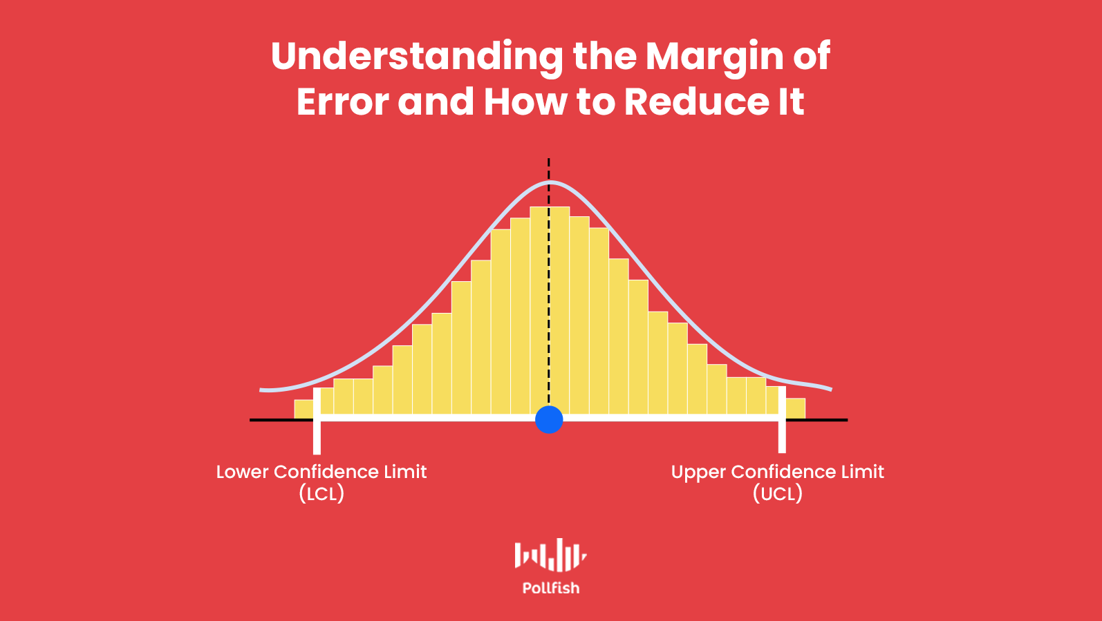
You may have pondered, what is the margin of error during your survey research, as this figure is sure to come up when analyzing data and forming an accurate reading of survey results.

In survey research and statistics, this pesky error rears its ugly head omnipresently. Commonly called the margin of error, this phenomenon is also referred to as the confidence interval. Despite the latter name, it is in the best interest of researchers to keep this metric low.

This is because, no matter who you survey or how many people, it is impossible to garner responses that represent everyone in the target population of your study. This is where the core of the margin of error lies, as it shows researchers how much of a survey’s results represent the views of its target population.

This article explains what is a margin of error and how to reduce it in your survey.

Defining the Margin of Error

The margin or error  — or the confidence interval — is a measurement of error in the results of a survey, specifically one that relies on the random sampling method . This metric shows researchers the degree to which they can expect survey results to reflect the views of the overall studied population.

As aforesaid, it is imperative to keep the margin of error low , as a high one points to a smaller likelihood of survey results to reflect the true views of your target population. As such, a higher margin of error renders your survey less reliable and inconclusive.

Moreover, a higher confidence interval (a misnomer as it may be) makes your survey unable to be used for statistical methods, such as in quantitative studies . It also debilitates descriptive and qualitative research . 

Researchers should thus aim for a lower margin of error, as it denotes higher confidence of a survey results’ accuracy, whereas a higher one signifies the opposite. 

The Utility of Studying the Margin of Error

While this statistic may be a frustrating reality in survey research, it is crucial to keep track of it. This is because survey data, necessary and enlightening as it may be, is imprecise. Why? Because survey samples represent a chunk (usually a small one) of your target population, and an even smaller one if it is in relation to your entire target market. 

Since a sampling pool (survey respondents) represents a larger population, there will always be the presence of uncertainty and imprecision. 

The confidence interval is useful in that it calculates this inherent imprecision to allow researchers to see how trustworthy their survey results are in representing a certain population.  

Additionally, the margin of error helps researchers determine the accuracy of a value, by expressing it in a range . The margin of error supports this, since the resulting answers of a survey question get assigned a percentage for statistical survey analysis. 

But since it is impossible to survey every last member of a target population, this percentage is only representative of the sampling pool . The margin of error allows this percentage to be expressed as a range to more accurately represent the answer in relation to the entire target population.

For example, if a survey’s results show that 40% of respondents sit while listening to music, this figure is incomplete. When you calculate the margin of error, on the other hand, it helps turn this figure into a more precise representation. If the margin of error turns out to be 4%, the percentage of 40% can be expressed as a range of 36-44%.

How to Calculate the Margin of Error

Calculating the margin of error requires plugging in a few variables into a formula. These include your sample size and the population standard deviation . The latter variable requires a calculation of its own. 

The standard deviation is a measure of the spread of scores in a data set that pertains to a specific population. A low standard deviation entails that most of the scores are closer to the average one, while a higher standard deviation shows that the scores are more dispersed. In short, this metric is also used for the purposes of data reliability.

These variables are just a few of the key aspects of calculating the margin of error. Below is the formula in its entirety.

The Formula Explained in Steps:

• Find the population standard deviation (σ) and determine your sample size (n).
• Get the square root of your sample size.
• Divide the population standard deviation (σ) by the result of the square root calculation.
• Multiply this result by the z-score that corresponds with your desired confidence level — not to be confused with the confidence interval (which is the margin of error). 

*Use the table below to find the z-score.  

How to Reduce the Margin of Error

As a researcher or business owner studying your target market, you are probably wondering how to reduce the margin of error. After all, a more reliable survey is going to be far more useful and one less obstacle to contend with. 

Here are several best practices to input into your survey research, to reduce the confidence interval. This will help make individual answers, as well as their ensuing variables (such as mean and average), become more precise. 

• Do this by changing how you gather the data. Ex: make precise measurements, make your process more orderly.
• Bear in mind that a larger sample size may require more time and resource allocation. 
• You should thus only lower the confidence level if the benefit of more precision (a reduced margin of error) outweighs the disadvantage of a lessened confidence level. 
• Example: If increasing the sample size is too costly for you, then lower the confidence level for a decreased confidence interval. Just remember, your confidence level has declined.
• Implement a one-sided confidence interval. This has a smaller margin of error than a two-sided confidence interval. This interval signifies only if a parameter is either smaller than or greater than a cut-off value. 
• It doesn’t show any information about the parameter on the opposite side. As such, use this to increase an estimate’s precision of an estimate only if you fear the estimate will be greater or less than a cut-off value, i.e., not both.

Using the Correct Survey Platform

Can using a strong online survey tool help decrease the margin of error? The answer is rather complicated. On one hand, a strong survey tool will help you avoid inaccuracies (think gibberish answers, straightlining, etc.) and illogical questions. It can also help ambiguity with open-ended questions.

These aspects are certainly crucial in helping eliminate ambiguity. But there are things that affect the margin of error that a survey simply has no control over.

For example, the population size and confidence level are factors outside of a survey and its hosting platform. 

With this in mind, you should understand that the margin of error cannot be fully diminished. It is impossible to perfectly align with the population you’re surveying. Especially when certain respondents have a tendency to change their minds. However, you can still determine how close you are to precisely reflecting their views by determining the margin of error yourself, or by calculating it with a designated tool (such as the one hyperlinked at the very beginning of this article).

What’s most important about an online survey platform is that it can deliver peace of mind on so many aspects that go into survey research , minimizing the labor that you need to exert into your studies and making the process much smoother and easier when it comes to reaching results (and analyzing them). 

Do you want to distribute your survey? Pollfish offers you access to millions of targeted consumers to get survey responses from $0.95 per complete. Launch your survey today.

Privacy Preference Center

Privacy preferences.

An official website of the United States government

The .gov means it’s official. Federal government websites often end in .gov or .mil. Before sharing sensitive information, make sure you’re on a federal government site.

The site is secure. The https:// ensures that you are connecting to the official website and that any information you provide is encrypted and transmitted securely.

• Publications
• Account settings

Preview improvements coming to the PMC website in October 2024. Learn More or Try it out now .

• Advanced Search
• Journal List
• v.15(1); 2023 Jan

Common Statistical Errors in Scientific Investigations: A Simple Guide to Avoid Unfounded Decisions

Alessandro rovetta.

1 Research and Disclosure Division, R&C Research, Bovezzo (BS), ITA

During my experience as an author, peer reviewer, and editor during COVID-19, I have encountered - and committed - various errors related to the interpretation and use of statistical measures and tests. Primarily concerning health sciences such as epidemiology, infodemiology, and public health, the evidence used to inform a conclusion carries an extremely high weight as it translates into decisions made to preserve the population's well-being. Therefore, the aforementioned evidence must be reliable. This short guide discusses the most common and dangerous mistakes I have experienced during my scientific journey. Real and invented examples have been proposed and analyzed in detail, showing possible interpretations, both correct and incorrect, and their consequences. Such a framework makes it clear that a statistical test alone cannot answer any scientific questions. Indeed, the interpretation of results and the verification of assumptions and test eligibility - subject to the author's evaluation - are crucial components of the integrity of the scientific investigation. Before using a test or adopting a measure, we must ask ourselves the following fundamental questions: Are there valid reasons to explore my research question? Am I sure my approach can fully and adequately answer my research question? Am I sure that my model's assumptions - basic and hidden - are sufficiently satisfied? How could violating those assumptions affect the validity of the results and stakeholders? Is the effect size relevant regardless of statistical significance?

Introduction

During the COVID-19 crisis, between May 2020 and December 2022, I published several peer-reviewed articles, carried out hundreds of peer reviews for over dozens of scientific journals, and edited various manuscripts for a couple of journals. In this experience, I noticed a recurrence of errors (including mine) concerning the use and interpretation of statistical measures and tests. In this regard, numerous authors have extensively addressed similar problems. For example, Greenland et al. thoroughly analyzed various errors in interpreting P -values and confidence intervals (CIs) [ 1 ]. Nonetheless, in this paper, I try to summarize and explain, most simply, the principal mistakes I pointed out during the last two years. In this scope, I adopt real and realistic health-related examples. In particular, I made this paper to provide a guide to help authors (including myself) develop more robust manuscripts and achieve more solid conclusions. Although correct data and calculations are unlikely to be useless or harmful to the scientific community, misinterpretations of the latter pose a severe threat to public health.

Technical report

CIs and statistical thresholds

It is too widely believed that overlapping 1 - α CIs (e.g., 95% CI) imply P > α (e.g., P  > 0.05). Here, we quickly prove that this implication is simply not true. For example, we apply the Welch t-test for the following average values ( N  = 100): X  = 0 (SD 0.05) and Y  = 1 (SD 0.5). The 95% CIs are (-0.10, 0.10) and (0.02, 1.98), i.e., they overlap (intersection size 0.08). Nonetheless, the test result is P  = 0.049 < 0.05 = α . It can be proved that nonoverlapping 1 - α  CIs imply P  < α ; however, as extensively discussed in the literature, obsession with significance thresholds should be discouraged (indeed, P = 0.049 and P = 0.051 are practically identical values) [ 1 ].

Statistical significance and effect size

On too many occasions, the existence and relevance of a certain phenomenon are attributed to a related statistical significance. Although this is wrong for various purely theoretical reasons (for instance, statistical significance regards the test adopted and not the phenomenon), here we focus on a more practical aspect: the applicability of a decision made by evaluating only statistical significance. Suppose my cardiologist recommended I lose weight significantly so as to reduce the risk of a heart attack. Thus, I measured my weight weekly for 10 weeks, obtaining the values ​​shown in Table ​ Table1 1 .

Applying a linear regression model, I found that the residuals were sufficiently compatible with the hypotheses of distributive normality (Shapiro-Wilk test P  = 0.67) and constant variance, also known as homoskedasticity (White test P  = 0.28). As the model was reliable, the slope of -0.07 kg/week (SE 0.01) - which strongly supported the negative trend - was very significant ( P  = 0.0001). Nonetheless, when I presented these highly significant findings to my cardiologist, he was hospitalized for a heart attack due to a fit of anger (sarcasm). Indeed, I believe that, however significant these results were, the 700 g lost in 10 weeks was not the health goal set.

Multicomparison adjustment of P -values

Adjustment for multicomparison is often necessary to reduce the number of false positives but introduces the risk of increasing false negatives. Hence, as in the previous case, its implementation must be assessed on a case-by-case basis. For example, if my objective is to detect anomalies that are potentially very dangerous to public health (e.g., via metal detectors in an airport), it is better to have a high number of false positives (false alarms of armed persons) than a high number of false negatives (which is equivalent to not identifying armed individuals). Conversely, if my purpose is to conduct an exploratory investigation (e.g., to look for causal correlations between various theoretically unrelated phenomena), then it can be crucial to avoid the so-called look elsewhere effect  and reduce (but not eliminate) spurious associations. A real-world example concerning Bonferroni correction is reported in the next section.

Inferential and descriptive statistics

Let's start with a real example, which is the number of annual deaths in Italy from 2015 to 2021 (data taken from ISTAT [ 1 ]). Considering that there is high data compatibility with the hypothesis of normality from 2015 to 2019 (Shapiro-Wilk test P  = 0.54) and we do not detect clear historical trends in that period, we calculate the average number of deaths between 2015 and 2019 ( X ) and compare it with those ​​of 2020 (Y1) and 2021 (Y2). After that, we subtract this average from all dataset values ​​in order to have the number of excess deaths, obtaining the new measures X  = 0 (SD 13,400, SEM 6,000, range [-19,000; 13,500]), Y1 = 100,000 (95% CI [88,000; 112,000]), Y2 = 63,000 (95% CI [51,000; 75,000]). Grubbs tests for (Y1, X ) and (Y2, X ) returned P  = 0.007 and P  = 0.04, respectively. Although these numbers are merciless and unambiguous, we now show how choosing an inappropriate test and/or adjustment can produce dangerous false negatives. For instance, implementing the Bonferroni correction (and for only two tested hypotheses), we get P  = 0.01 and P  = 0.08. Again, this makes it clear that the evaluation of the effect size must be totally separated from statistical significance and P -value adjustment is not always the best choice. Indeed, in the context of public health, the 63,000 excess deaths, taking into account both the narrow CIs and minimal data variability from 2015 to 2019, represent an extraordinarily alarming figure despite its statistical significance. But that's not all - even admitting a larger variability, statistical fluctuations capable of creating such high excesses are a major public health situation (that can lead, for example, to hospitals' overcrowding).

Models' assumptions

Statistical tests and models are reliable only when their assumptions are sufficiently compatible with our data. Too often, little importance is given to this aspect, which is absolutely essential for drawing valid scientific conclusions. For example, Figure ​ Figure1 1 shows three different outliers (blue, orange, and gray dots) for the same dataset (light-blue dots) and the associated linear correlations. As the use of the Pearson correlation standardly requires distributive normality (which implies the absence of outliers), it is evident that these results are biased (if the aim is to find a global linear relationship). The correlation value increases as the outlier increases. The associated P -values ​​are 0.005, 0.02, and 0.17.

In this regard, it is important to underline that P -values ​​are biased downward as they signal not the correlation significance but the violation of the normality assumption (i.e., they signal that the data are poorly compatible with the test hypothesis assumptions rather than the test hypothesis itself). Another example concerns homoskedasticity in linear regression models: indeed, its violation does not compromise the validity of the model but only the estimation of errors and the P -values. This can be seen in Figure ​ Figure2 2 (blue line): the data are very compatible with residual normality (Shapiro-Wilk test P  = 0.48) but not with homoskedasticity (White test P  = 0.001; the problem could be overcome by applying a weighted regression). Nonetheless, the linear behavior of the data is evident; thus, the model could still be useful for making decisions without considering inference and statistical errors.

Correlation value and slope

Phenomenon and correlation intensity are two different and generally independent aspects. As shown in Figure ​ Figure2, 2 , the correlation value is not related to the function slope: indeed, the blue line has a greater slope (about 4) than the orange line (about 2) despite its R2 being markedly lower (0.77 versus 0.99).

Hypothesis targeting and causation

Suppose I present the following real data to you without specifying what they represent (Figure ​ (Figure3 3 ).

Applying the usual linear regression model, it turns out that there is little evidence against distributive normality and homoskedasticity (Shapiro-Wilk test P  = 0.28, White test P  = 0.21). Furthermore, the correlation is marked ( R  = 0.97, 95% CI [0.91, 0.99]) and highly significant ( P  < 0.0001). It seems reasonable to conclude that at least one of the two variables affects the other or if the correlation is spurious, there is a confounding factor that affects the two variables similarly. Nonetheless, the two variables are the annual US money invested in science, space, and technology and the number of suicides by hanging, strangulation, and suffocation [ 2 ]. This shows an obvious but often underestimated fact: statistics alone can never provide evidence of causation. The targeting of a research hypothesis - understood as the set of evidence and reasoning that make a hypothesis worthy of research - is an essential part of any scientific investigation (including exploratory studies). Other misinterpretations concern Granger causality: indeed, Granger causality is not true causality [ 3 ]. For example, by searching Google Trends for the queries batman  (comics superhero) and pogba  (soccer player) [ 4 ], we get the following graph (Figure ​ (Figure4). 4 ). We apply the Granger causality with time lag = 11 weeks (one degree of nonseasonal differentiation for both series) and find ample evidence against Y ≠ f ( X ) ( P  = 0.002). Therefore, we should conclude that the web interest in Batman predicts the web interest in the soccer player Pogba, which is very unlikely (Google Trends-related queries confirm the absence of a causal relationship).

CIs and data variability

In many papers, it is customary to report CIs as an estimate of the precision of the measurement/calculation. While they are necessary to assess the relevance of the effect size, confidence (or credible) intervals concern the distribution of the average values; hence, in general, they do not provide information on the dataset variability. Proof of this can be easily obtained from the following example: Suppose we have a Gaussian dataset of 100 elements with an SD of 20 and another Gaussian dataset of 9 elements with an SD of 9. Both datasets have mean values equal to 0. The 95% CIs are (-4, 4) and (-6, 6), respectively. Therefore, the CI of the first dataset is narrower than the second despite its considerably larger SD. Again, we must always ask ourselves what our research purpose is and how our data and analysis characteristics can affect stakeholders.

Central limit theorem

The central limit theorem is often invoked to state that a dataset has Gaussian characteristics as it is sufficiently numerous (e.g., N > 30). However, this is simply wrong and misleading. Indeed, the central limit theorem concerns only the population of the mean values and not the original population or sample [ 5 ]. It follows that it is useful for applying parametric tests, but it does not justify the adoption of descriptive statistics such as mean, variance, or SD for non-Gaussian datasets. In this regard, an easy counterexample can be proposed: considering the dataset of 1250 elements shown in Figure ​ Figure5, 5 , the Shapiro-Wilk test returns P  < 0.0001. Moreover, the percentage difference between the median and mean is equal to 78.1%. Finally, the average value is outside the dataset. In conclusion, this dataset is extremely non-normal.

Mixed use of different tests: a precautionary note

It is a common practice to use different tests to measure the significance of discrepancies between similar datasets. For example, if the purpose is to compare three pairs of datasets, of which two are normally distributed, and one is not, then some authors may choose two parametric tests and one nonparametric test, respectively. Nonetheless, it is essential to consider that these tests might not only measure different quantities or the same quantity in different ways but that tests' assumptions and the sensitivity to their violation could also be very different. Thus, the same exact P -value (e.g., P  = 0.02) obtained from two different tests could imply a very different degree of statistical significance and meaning (of course, this could also happen even when the same test is applied multiple times, but the chance is lower according to what discussed above). Consequently, when the purpose is to inform a single set of decisions, adopting mixed tests could create a heterogeneity capable of strongly biasing the results. In this regard, considering these aspects in the analysis and the related uncertainty in the final conclusion is imperative.

Counterfactual scenarios

Evaluating a counterfactual scenario is one of the most complicated and important tasks in science. For example, if the objective is to estimate the impact of COVID-19 on mortality, it is necessary to make a prediction - without COVID-19 - based on the previous historical trend (e.g., the prior 5 or 10 years). This assessment is entirely based on the assumption that a trend remains unchanged in the absence of significant external events (the principle of parsimony). While this assumption is reasonable, and the history of science confirms its validity, a moderate degree of uncertainty must be considered. For instance, the superposition of nonlinear trends could give rise to a linear trend up to a certain date (threshold) and a nonlinear trend beyond the latter (Figure ​ (Figure6). 6 ). If the external event occurs in conjunction with the threshold, an improper causal association could be asserted (this is not the case with COVID-19 impact on mortality [ 6 ]).

Source: [ 6 ]

Moreover, the external factors could be multiple, which makes it difficult to identify which of these was predominant for the change in trend. For these reasons, once again, the scientific targeting of the hypotheses is fundamental for the investigation's validity. Indeed, only the combination of evidence from various disciplines can provide solid conclusive evidence. On the other side, this exposes the research more to authors' bias [ 7 ]. Finally, it is possible to obtain different results by observing different temporal windows to make comparisons. For example, the statistics on excess deaths in Italy during 2020 are slightly different if we consider the previous five years as a comparison time-lapse instead of the previous 10 years [ 6 ]. This happens because all the real models have a margin of uncertainty, and it is not always easy to select the correct width of the temporal window.

Hidden assumptions

Suppose we need to measure the impact of the COVID-19 pandemic on web interest in porn [ 8 ]. Thus, exploiting the central limit theorem, we apply a Welch t-test between the 2017-2019 and 2020-2022 datasets, obtaining a high (7.4, 95% CI 6.0-8.9) and significant (P<.0001) negative decrease due to COVID-19. Since the test's assumptions have been met, it could be concluded that the result is reasonable. However, comparing statistics such as mean and median requires a fundamental implicit assumption that there are no trends and seasonality in the time series (i.e., there is sufficient stationarity). Indeed, an evident downward trend was already underway before COVID-19 (Figure ​ (Figure7). 7 ). Nevertheless, while the result found is not surprising despite its low P -value (i.e., it is in line with the predictions or, at best, cannot answer the research question), it is still helpful to support the presence of a historical decreasing trend and quantify the global decrease.

Wrong choice of test for the goals of analysis

Suppose we want to measure the change in average daily particulate matter (PM) 2.5 concentrations during two specific weeks of two consecutive winters in a certain area. For this example, we assume that no historical trends were in place. Data were considered sufficiently normal (Shapiro-Wilk test  P = 0.35) to adopt the one-sample t-test on the paired differences (Table ​ (Table2 2 ).

*Critical value for public health.

CI, confidence interval; PM, particulate matter

The test result provides little evidence against the difference in the paired differences of PM 2.5 concentrations ( P  = 0.09). Hence, the two distributions could be considered similar. Nonetheless, we must ask ourselves: Are we applying the proper test for this public health assessment? The answer is no as exceeding some critical PM 2.5 concentrations ​​poses a more serious threat to health [ 9 ]. Indeed, the safety values ​​were exceeded in 6 out of 14 days in the 2020 series. In this regard, the negative lower limit of the 95% CI suggested that the test had poor accuracy due to the high variance of 2020 (CV1 = 43% versus CV2 = 17%). Another known but noteworthy case is that of the Mann-Whitney U test, which is frequently used to measure the significance of the difference between two medians or distributions. As has also been shown in other literature, this can be wrong in many ways [ 10 ]. Indeed, the Mann-Whitney test ranks all the values from low to high and then compares the mean ranks; therefore, it is sensitive to data spread [ 11 ]. It can be used to compare medians (and even means) only when the distributions of the two populations have the same shape. Thus, in this case, it is not a matter of the test’s assumptions but the analysis' goal.

Comparison of results

Suppose we have two independent samples of N  = 10 elements that sufficiently meet all the assumptions for using the Pearson correlation properly. The two correlations have values x  = 0.70 (95% CI 0.13-0.92; P = 0.02) and y  = 0.50 (95% CI -0.19 to 0.86; P  = 0.14). Based on these P -values, we conclude that the first correlation is much more significant than the second. This could lead us to say there is a substantial difference between the two correlations. Nevertheless, comparing their values ​​with the method of Eid et al. [ 12 ], we get P  = 0.28. Therefore, as also underlined by the large CIs, there is little evidence against the equality of the two correlations. This shows that to make claims about the comparison of two (or more) results, we must directly compare them through an appropriate test (or evaluate their effect size) and not rely on their single statistical significance.

Multicomparison adjustment to inform a final decision

One of the most common errors is to believe that the adjustment for the multicomparison should only be applied when the results or data are directly compared with each other (e.g., as done in the Comparison of Results section). Indeed, the adjustment for the multicomparison - when deemed appropriate - should be made when the final decision (e.g., to apply a lockdown based on the abnormal increase in flu symptoms among a population) is based on the result of multiple tests, regardless of whether these tests are mutually comparative or independent [ 6 ]. As a matter of fact, the increased likelihood of false positives is due to the high number of tests used and not to the nature of the latter [ 13 ].

Presentation of results

As also done in this paper, we often talk about test results as if they were properties of the dataset (e.g., the values ​​are normally distributed). This approach is technically inaccurate as applying different tests could produce different results. Indeed, the P -value is related to the test adopted and not the dataset itself. To prove this, we consider the following vector X  := (-14, 0, 1, 2, 3, 5, 6, 7, 9). If we apply the Shapiro-Wilk test to its components, we obtain P  = 0.03, which suggests that the dataset is not normal (i.e., there is low compatibility with the normality hypothesis). On the contrary, if we apply the Kolmogorov-Smirnov test, we obtain P  = 0.51, which suggests that the dataset can be considered normal (i.e., there is high compatibility with the normality hypothesis). However, this slight terminology abuse could be tolerated as long as the test adopted to evaluate the dataset compatibility with the fixed hypothesis is clearly specified.

This brief overview provides practical indications for epidemiological analysis and public health surveillance strategies. It has been proven that overlapping CIs do not imply exceeding the significance threshold (while it is true that nonoverlapping CIs imply P -values ​​lower than the threshold). However, as P -values are graded measures, the adoption of significance thresholds should be discouraged. Statistical significance, when properly used, provides information on how compatible ( P -values) or surprising ( S -values = -log( P -value, 2)) the results found are compared to the test hypothesis adopted through the chosen test, but, in general, it does not provide information on the effect size. Therefore, the intensity of a phenomenon or the importance of an outcome must be assessed separately according to the scientific goal, context, and stakeholders (especially when public health is involved). Adjustment for multicomparison should be evaluated according to the scientific or even ethical relevance of the decision to be informed (e.g., conservation of public health). Comparing two or more results based on their single significance is unreliable and potentially very misleading, as only a comparative test or a specific evaluation of their effect sizes provides information on their mutual relationship. If considered appropriate, the adjustment for multicomparison should only be applied based on the number of tests used to inform the final scientific decision and not on the type of test performed. In particular, it is not necessary for the test to directly compare two or more outcomes or data to require adjustment for multiple comparisons. Descriptive and inferential statistics offer different clues to inform public health or any other scientific decision. In particular, inferential statistics do not always fit into the context of public health surveillance. The metal detector approach should be enforced during health crises (especially when the available data is little) to counter or prevent their effects. Verifying the models' assumptions and evaluating the effects due to their violation is crucial to draw scientifically valid conclusions. Reviewers and editors of all academic journals and agencies should specifically request a thoughtful description of how these aspects were managed in a manuscript. Assuming that all the appropriate assumptions are verified, the correlation value provides information on how well the data is positioned along a line (e.g., Pearson) or other function (e.g., Spearman). However, the slope of these functions is a different and generally independent aspect. The hypothesis targeting is the basis of any scientific exploration; indeed, no statistical analysis (including Granger causality or similar) can provide evidence of causation without the latter. CIs and credibility intervals provide information on the distribution of mean values ​​but not on the variability of the dataset. This aspect must be considered according to the purpose of the analysis. Furthermore, it is always necessary to ask which characteristics of our data are relevant to inform the final decision and stakeholders. The central limit theorem guarantees the normality of the distribution of the mean values ​​of a sufficiently large dataset but is in no way valid for the dataset itself. The dataset's characteristics must be evaluated using appropriate tests and graphical representations according to the research purpose. The test used in this scope must always be clearly specified since P -values regard the test and not the dataset. Mixing different types of statistical tests to analyze similar datasets can lead to marked heterogeneity of scenarios, which can compromise the validity of the conclusion based on these tests. Carefully evaluating this aspect is fundamental to guarantee the scientific integrity of the whole research and inform the final decision properly. The evaluation of a counterfactual scenario is complex and always subject to a nonnegligible margin of unavoidable uncertainty. Therefore, hypothesis targeting and scientific rationale are key factors in determining a counterfactual model's validity and plausibility. When we use a statistical test, we don't just have to verify its standard assumptions but also ask ourselves if our data are suitable for applying such a test to respond to our research question. Moreover, when we use a statistical test, we must adequately consider whether this is suitable to help us in responding to our research question. Indeed, even if all assumptions (both primary and hidden) are verified, mere statistics cannot provide solid evidence for or against its use for a given scientific objective.

Conclusions

This framework makes it clear that a statistical test alone cannot answer any scientific questions. Indeed, the interpretation of results and verification of assumptions and test eligibility - subject to the author’s evaluation - are crucial components of the integrity of the scientific investigation. Therefore, before using a test or adopting a measure, we must ask ourselves the following fundamental questions: Are there valid scientific reasons to explore my research question? Am I sure my approach can fully and adequately answer my research question? Am I sure that my model's assumptions - basic and hidden - are sufficiently satisfied? How could violating those assumptions affect the validity of the results and the stakeholders? Is the effect size relevant regardless of statistical significance?

The content published in Cureus is the result of clinical experience and/or research by independent individuals or organizations. Cureus is not responsible for the scientific accuracy or reliability of data or conclusions published herein. All content published within Cureus is intended only for educational, research and reference purposes. Additionally, articles published within Cureus should not be deemed a suitable substitute for the advice of a qualified health care professional. Do not disregard or avoid professional medical advice due to content published within Cureus.

The authors have declared that no competing interests exist.

Human Ethics

Consent was obtained or waived by all participants in this study

Animal Ethics

Animal subjects: All authors have confirmed that this study did not involve animal subjects or tissue.

Sample Size Calculator and Margin of Error: The Ultimate Guide by Appinio

Appinio Research · 20.12.2022 · 19min read

Whether it's about political sentiment, customer satisfaction, the Appinio Hype Train or a company employee survey, surveys are the most common way to find out public sentiment, opinions, beliefs and tendencies. And of course the more people you ask questions to, the closer you get to a representative result. But imagine interviewing all the people in the UK to find out who they would vote for in the next election, impossible!

This is where the need of a representative sample comes into play.

A representative sample focuses on a portion of the population and aims to reflect the views of the general public. But, especially in survey research, what variables do you need to take into account? How do you know how many survey respondents you require to ensure you survey a representative sample of the population? In this article, we’ll show you which key values you need in order to calculate the perfect sample for your study and how accurately your results represent the population.

Do you want to calculate the sample size for your study quickly and already have all the key values? Then use our online sample size calculator margin or error to determine the sample you need.

Sample size calculator

Use our calculator to quickly check the sample size for your study. Just enter your values and check the result. All metrics used in the calculator are explained in detail later in the article. If you have more questions, feel free to reach out to

our experts via the chat.

Definition: What is a sample?

A sample is a small portion or quantity intended to show what the whole is like.

There are several different methods of sampling that can be used, for example, you could choose to use a “random sample,” where respondents are chosen entirely by chance from the population at large, therefore every member of the population has an equal chance to be selected for your study.

A random sample is useful when doing exploratory market research or gathering new ideas, but it would not be useful if you wanted to know how many Brits are vegan, as your random sample could exclude some participants (e.g. not enough women) or include too many people from the same group (e.g. too many Millennials), therefore, you would not be able to extract insights that are applicable to your desired target group or the general population.

The reason why sample size is important

That's why, in survey research especially, a sample needs to meet specific criteria and contain all the different groups - such as women, men or different age groups - in the same proportions to the population you want to represent. In addition, the sample should be large enough not only to be representative, but also to make reliable statements. When choosing a sample it is important to test its reliability, if a sample is too small the information collected may be partial, on the other hand if the sample is too large it would be a waste of resources. The larger the group, the closer are results to the target market, the less chance factors, errors and false statements can distort the result. The results are considered representative of the whole itself, i.e. applicable to the general public, when they reflect the normal distribution in the population

If you want to get survey data that is as reliable as possible, you need to strive to make your survey representative. In market research, you need to collect data from the target group before launching a product on the market in order to offer a product that consumers will want to buy or use. However, you can't ask every potential buyer their opinion, it would simply be too time-consuming and not cost-effective. Moreover, it is impossible to determine exactly the size of the potential buyer group. Therefore, before sending your survey out to your respondents, you need to define a sample size that represents your target population as closely as possible, and in all its facets.

How large should a sample be?

The larger the sample size, the more accurate results are, right?

Generally, the larger the sample, the more representative it is, that is under the condition that we are surveying the right people; namely, we won't survey men when we want to represent pregnant women.

The results of a survey are considered representative when the outcomes of the survey accurately reflect the overall population which means that you can draw reliable conclusions about the general population as all characteristics of the target population are also present in your sample.

So a larger sample makes reaching representativeness easier, but on the other hand, the larger the sample size, the more expensive and time-consuming your survey will be. So, how can you balance costs and representativeness?

In order to do this, you must make trade-offs between the size of the sample and the margin of error, namely, you have to find a sample size that is large enough to achieve the desired level of precision and stay within an acceptable margin of error.

Let’s have a look at the margin of error metric and what margin of error is considered acceptable.

What is the margin of error?

The margin of error (or marginal error) is a statistic expressing the amount of random sampling error in the results of a survey. The larger the margin of error, the less confidence one should have that a poll result would precisely reflect the result of a census of the entire population. The margin of error relates to the size of your sample and the difference between results from your survey data and those from population (normal) distribution, it tells you how close your results reflect the views from the overall population. Let's make an example.

As you can guess by the word margin, the margin of error is a range of values around the sample mean. For example, a survey of 1000 people of your targeted population gives you a 5% margin of error, meaning that 95% of the time the results are within 5% range of what they would be if you had asked every single person in your target population. Thus, if your survey data indicates that 40% of the total population approve or disapprove of something, the margin of error means that you can be 95% confident that the true figure falls between 35% and 45%. The marginal error indicates how close the results of the sample are to reality. This can be calculated by taking into account the sample size, margin of error and confidence level. The marginal error should not be too high, otherwise it can lead to wrong conclusions which could have serious consequences. An acceptable margin of error used by most survey researchers typically falls between 4% and 8% at the 95% confidence level. It is important to keep the margin of error as low as possible as the smaller the margin of error, the more confidence you may have in your results, the bigger the margin of error, the farther they can stray from the views of the total population, making your results unusable. As a rule of thumb, as sample size grows marginal error decreases but, it should be noted that a too large sample size makes the survey more expensive and time consuming. Therefore, finding a balance between marginal error and sample size is essential. With proper planning you can make sure that your sample is representative of the target population, with marginal errors as low as possible so your results are accurate and reliable.  Let’s keep in mind that what is considered an acceptable value also depends on the kind of research you’re conducting. For obvious reasons, medical studies and trials have higher standards and stricter criteria when it comes to sampling and collecting results than researching consumers' purchasing behaviour.

Margin of error calculator

Use our calculator to quickly check the margin of error for your study. Just enter your values and check the result. All metrics used in the calculator are explained in detail below. If you have more questions, feel free to reach out to our experts via the chat.

An acceptable margin of error used by most researchers typically falls between 3% and 6% at the 95% confidence level.

The key values to calculate sample size and margin of error

The key values to determine the optimal sample size and / or margin of error are the total population N, the standard deviation p, confidence interval (CI) and the Z-value z. Here is a brief explanation for every metric.

Standard deviation, p

When looking at survey results, you should be able to make general statements such as "xx% approve of this". However, this can vary greatly between respondents, which is why we also need to take into account standard deviation. Standard deviation is expressed in percentage and specifies the range of probable answers for each question. The higher this value, the more participants are needed to obtain an accurate result. The standard deviation value is usually set at 0.5 and indicates how much variation is expected in the answers of the respondents. Here's an example of how a high standard deviation can occur when using a Likert scale question: Imagine a survey is conducted to measure people's opinion on a new product. One of the questions is: How likely are you to recommend this product to a friend? Respondents reply via a Likert scale question with five options: "Strongly unlikely", "Unlikely", "Neutral", "Likely", "Strongly likely". Out of 100 respondents, 50 of them choose "Strongly unlikely" and the other 50 choose "Strongly likely". This means there is no middle ground in the responses, they are all at one of the two extremes. As we have half of the respondents choosing one extreme and the other half choosing the other extreme, the responses are not evenly distributed and the standard deviation would be much higher to indicate the large difference or spread between the responses. This high standard deviation is unusual when compared to a "normal" distribution of responses, where you would expect most responses to be close to the average, with fewer responses at the extremes. It is important to notice that a standard deviation value of 0.5 is considered a common value and typically only needs to be adjusted in edge cases, like the one mentioned in this example. If you have a specific use case in mind and are unsure on what kind of standard deviation to expect, you can also contact our experts for support.

Get a free demo and see the Appinio platform in action!

Z-score, z, and Confidence interval, (CI)

The Z-score measures how well the sample represents the total population (including the margin of error) and describes the deviation of a value from the average of your sample. Or in other words: The Z-value indicates how certain you could be that your study results correspond to reality. 

As it is more tangible, confidence intervals that represent a certain z-score are usually used for calculating a desired sample size or margin of error. This table shows the z-scores for the most common confidence intervals.

A confidence interval is a range of values, derived from a sample, that is used to estimate an unknown population parameter. It provides a level of certainty or confidence that the true population parameter falls within the interval.  The interval is calculated by taking a sample statistic (such as the mean or proportion) and adding and subtracting a margin of error, which is determined by the level of confidence desired and the sample size. The level of confidence is typically expressed as a percentage, such as 90%, 95%, or 99%.

The confidence interval is the range of values you expect your estimate to fall between if you redo your test, within a certain level of confidence.

Let’s use a visual example using a normal distribution.

For example, the probability of the population mean value being between -1.96 and +1.96 standard deviations (z-scores) from the sample mean is 95%.

Accordingly, there is a 5% chance that the population mean lies outside of the upper and lower confidence interval (as illustrated by the 2.5% of outliers on either side of the 1.96 z-scores).

Total population, N

In most everyday uses, the word population implies a group of people or at least a group of living beings. However, statisticians and researchers refer to whatever group they are studying as a population . The population of a study might be mothers of children under the age of 5 years old, doctors or users of a specific product. In order to draw the most precise conclusions possible, statisticians and researchers would need to know all the characteristics of the people in the desired population, but this is impossible or impractical most of the time, since population sets tend to be quite large. That’s why they select samples of the population, namely a smaller group drawn from the total population that has the characteristics of the entire population, so that the observations and conclusions made against the sample data can be attributed to the population as a whole. In our Appinio calculator we do not consider the total population as for most studies the population size is so large (e.g. all Germans) that it doesn’t affect the required sample size or margin of error. Only when the population you want to investigate is extremely small - like all male dentists in London - the total population needs to be taken into account. In this case you can check out our advanced formula below or directly consult our experts for help.

Open live chat

The case of unknown population

In most cases, determining the population size precisely is not possible, because it is too large and broad. In these cases, you can only use the upper part of the standard formula to calculate the minimum sample size:

Formula for determining the sample size

For completion’s sake, we are also going to show you how you can calculate the appropriate sample size using the extended formula, but if you are not a fan of maths and formulas bring back school memories that you’d like to keep hidden, use our Appinio calculators above. Once you determine all key values mentioned above, you can use the equation below to determine the optimal sample size. The following standard formula is best suited for small to medium population sizes.

Conclusions

In conclusion, a reliable sample size is critical for making accurate, representative and meaningful conclusions when conducting survey research. This ensures that marginal errors are minimised and that results can be extrapolated from the population with greater certainty. By following the outlined formula, you can determine the optimal sample size for your study to ensure accurate and reliable results.

We have discussed marginal error, sample size and the calculation of Z-value. To determine the sample size for a survey, you must use the standard formula and consider three key values: Margin of error, standard deviation, and Z-value. In specific use cases where you want to represent a very small population, population size needs to be considered additionally.  By following this formula, you can ensure accuracy and reliability in your survey results. The marginal error is a measure used to describe how well a sample represents the total population and refers to the likelihood of an error occurring. The Z-value is calculated based on the confidence level and indicates how certain you can be that your results correspond to reality. Finally, the sample size should be determined using the standard formula to minimise marginal errors and extrapolate results to the full population accurately.

Do you want to start your own survey but don't quite know how?

Have a look at the Appinio Hype Tracker Report! For the Appinio Hype Tracker Reports we investigate a population that is representative according to age and gender. Find all Appinio Hype Tracker volumes on our Report Page and register for the dashboard free of charge here.

Get free access to the platform!

Join the loop 💌

Be the first to hear about new updates, product news, and data insights. We'll send it all straight to your inbox.

Get the latest market research news straight to your inbox! 💌

Wait, there's more

17.04.2024 | 25min read

Quota Sampling: Definition, Types, Methods, Examples

15.04.2024 | 34min read

What is Market Share? Definition, Formula, Examples

11.04.2024 | 34min read

What is Data Analysis? Definition, Tools, Examples

• Salary & Income Tax Calculators
• Mortgage Calculators
• Retirement Calculators
• Depreciation Calculators
• Statistics and Analysis Calculators
• Date and Time Calculators
• Contractor Calculators
• Budget & Savings Calculators
• Loan Calculators
• Forex Calculators
• Real Function Calculators
• Engineering Calculators
• Tax Calculators
• Volume Calculators
• 2D Shape Calculators
• 3D Shape Calculators
• Logistics Calculators
• HRM Calculators
• Sales & Investments Calculators
• Grade & GPA Calculators
• Conversion Calculators
• Ratio Calculators
• Sports & Health Calculators
• Other Calculators

Margin of Error Calculator

This simple margin of error (MOE) calculator can be employed to compute the MOE of a survey in accordance with the sample proportion and size, and the desired confidence level.

You can use the calculator to compute the MOE in four simple steps:

• Use the drop-down menu to select the confidence level
• Input the sample size and then the proportion percentage
• If required, provide details of the population size
• Click on the "Calculate" button to generate the outputs.

The Margin of Error in Statistics

The majority of surveys that are conducted for research purposes are based on information that is collected from a sample population as opposed to the full population (a census). As the sample is only representative of the full population, it is likely that some error will occur, not in terms of the calculation, but in terms of the sampling. That is, a sampling error will emerge because the researchers did not include everyone that exists within a given population. The MOE measures the maximum amount by which the sample results may differ from the full population. As most responses to survey questions can be presented in terms of percentages, it makes sense that the MOE is also presented as a percentage.

Confidence Level (α) 70% 75% 80% 85% 90% 91% 92% 93% 94% 95% 96% 97% 98% 99% 99.5% 99.9% 99.99%

Sample Size (n)

Proportion Percentage (p)

Population Size (N) (optional)

Margin of Error Formula

The Margin of Error (MOE) Calculator uses the following formulas:

1.  MOE = z * √ p * (1 - p) / √ n

2.  MOE (with finite population correction) = z * √ p * (1 - p) / √ (N - 1) * n / (N - n)

MOE   is the margin of error,

z   is the z-score associated with a level of confidence,

p   is the sample proportion, expressed as a decimal,

n   is the sample size,

N is the population size.

To estimate the sample size, take a look at our sample size calculator .

Margin of Error Calculation Example:   A market research agency conducted a survey to identify how many mobile phone users use their devices to access social media. They surveyed 1000 mobile phone users and found that 540 regularly used their devices to access their social media profiles.

Let's assume that we require a 95% level of confidence; as such, the z-score = 1.96.

The sample population, p, is 540 / 1000 = 0.54. (The sample size, n, was 1000.)

As such, the margin of error in this survey is as follows:

MOE = z * √ p * (1 - p) / √ n

MOE = 1.96 * √ 0.54 * (1 - 0.54) / √ 1000

MOE = 0.977 / 31.623 * 100 = 3.089%

These results indicate that the market research company can conclude with 95% confidence that 54% of mobile phone users use their device to access social media, give or take 3%.

Reference: Daniel WW (1999). Biostatistics: A Foundation for Analysis in the Health Sciences. 7th edition. New York: John Wiley & Sons.

• Currently 4.78/5

Rating: 4.8 /5 (724 votes)