hypothesis testing calculator t value

t-test Calculator

Table of contents

Welcome to our t-test calculator! Here you can not only easily perform one-sample t-tests , but also two-sample t-tests , as well as paired t-tests .

Do you prefer to find the p-value from t-test, or would you rather find the t-test critical values? Well, this t-test calculator can do both! 😊

What does a t-test tell you? Take a look at the text below, where we explain what actually gets tested when various types of t-tests are performed. Also, we explain when to use t-tests (in particular, whether to use the z-test vs. t-test) and what assumptions your data should satisfy for the results of a t-test to be valid. If you've ever wanted to know how to do a t-test by hand, we provide the necessary t-test formula, as well as tell you how to determine the number of degrees of freedom in a t-test.

When to use a t-test?

A t-test is one of the most popular statistical tests for location , i.e., it deals with the population(s) mean value(s).

There are different types of t-tests that you can perform:

• A one-sample t-test;
• A two-sample t-test; and
• A paired t-test.

In the next section , we explain when to use which. Remember that a t-test can only be used for one or two groups . If you need to compare three (or more) means, use the analysis of variance ( ANOVA ) method.

The t-test is a parametric test, meaning that your data has to fulfill some assumptions :

• The data points are independent; AND
• The data, at least approximately, follow a normal distribution .

If your sample doesn't fit these assumptions, you can resort to nonparametric alternatives. Visit our Mann–Whitney U test calculator or the Wilcoxon rank-sum test calculator to learn more. Other possibilities include the Wilcoxon signed-rank test or the sign test.

Which t-test?

Your choice of t-test depends on whether you are studying one group or two groups:

One sample t-test

Choose the one-sample t-test to check if the mean of a population is equal to some pre-set hypothesized value .

The average volume of a drink sold in 0.33 l cans — is it really equal to 330 ml?

The average weight of people from a specific city — is it different from the national average?

Two-sample t-test

Choose the two-sample t-test to check if the difference between the means of two populations is equal to some pre-determined value when the two samples have been chosen independently of each other.

In particular, you can use this test to check whether the two groups are different from one another .

The average difference in weight gain in two groups of people: one group was on a high-carb diet and the other on a high-fat diet.

The average difference in the results of a math test from students at two different universities.

This test is sometimes referred to as an independent samples t-test , or an unpaired samples t-test .

Paired t-test

A paired t-test is used to investigate the change in the mean of a population before and after some experimental intervention , based on a paired sample, i.e., when each subject has been measured twice: before and after treatment.

In particular, you can use this test to check whether, on average, the treatment has had any effect on the population .

The change in student test performance before and after taking a course.

The change in blood pressure in patients before and after administering some drug.

How to do a t-test?

So, you've decided which t-test to perform. These next steps will tell you how to calculate the p-value from t-test or its critical values, and then which decision to make about the null hypothesis.

Decide on the alternative hypothesis :

Use a two-tailed t-test if you only care whether the population's mean (or, in the case of two populations, the difference between the populations' means) agrees or disagrees with the pre-set value.

Use a one-tailed t-test if you want to test whether this mean (or difference in means) is greater/less than the pre-set value.

Compute your T-score value :

Formulas for the test statistic in t-tests include the sample size , as well as its mean and standard deviation . The exact formula depends on the t-test type — check the sections dedicated to each particular test for more details.

Determine the degrees of freedom for the t-test:

The degrees of freedom are the number of observations in a sample that are free to vary as we estimate statistical parameters. In the simplest case, the number of degrees of freedom equals your sample size minus the number of parameters you need to estimate . Again, the exact formula depends on the t-test you want to perform — check the sections below for details.

The degrees of freedom are essential, as they determine the distribution followed by your T-score (under the null hypothesis). If there are d degrees of freedom, then the distribution of the test statistics is the t-Student distribution with d degrees of freedom . This distribution has a shape similar to N(0,1) (bell-shaped and symmetric) but has heavier tails . If the number of degrees of freedom is large (>30), which generically happens for large samples, the t-Student distribution is practically indistinguishable from N(0,1).

💡 The t-Student distribution owes its name to William Sealy Gosset, who, in 1908, published his paper on the t-test under the pseudonym "Student". Gosset worked at the famous Guinness Brewery in Dublin, Ireland, and devised the t-test as an economical way to monitor the quality of beer. Cheers! 🍺🍺🍺

p-value from t-test

Recall that the p-value is the probability (calculated under the assumption that the null hypothesis is true) that the test statistic will produce values at least as extreme as the T-score produced for your sample . As probabilities correspond to areas under the density function, p-value from t-test can be nicely illustrated with the help of the following pictures:

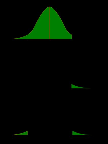
The following formulae say how to calculate p-value from t-test. By cdf t,d we denote the cumulative distribution function of the t-Student distribution with d degrees of freedom:

p-value from left-tailed t-test:

p-value = cdf t,d (t score )

p-value from right-tailed t-test:

p-value = 1 − cdf t,d (t score )

p-value from two-tailed t-test:

p-value = 2 × cdf t,d (−|t score |)

or, equivalently: p-value = 2 − 2 × cdf t,d (|t score |)

However, the cdf of the t-distribution is given by a somewhat complicated formula. To find the p-value by hand, you would need to resort to statistical tables, where approximate cdf values are collected, or to specialized statistical software. Fortunately, our t-test calculator determines the p-value from t-test for you in the blink of an eye!

t-test critical values

Recall, that in the critical values approach to hypothesis testing, you need to set a significance level, α, before computing the critical values , which in turn give rise to critical regions (a.k.a. rejection regions).

Formulas for critical values employ the quantile function of t-distribution, i.e., the inverse of the cdf :

Critical value for left-tailed t-test: cdf t,d -1 (α)

critical region:

(-∞, cdf t,d -1 (α)]

Critical value for right-tailed t-test: cdf t,d -1 (1-α)

[cdf t,d -1 (1-α), ∞)

Critical values for two-tailed t-test: ±cdf t,d -1 (1-α/2)

(-∞, -cdf t,d -1 (1-α/2)] ∪ [cdf t,d -1 (1-α/2), ∞)

To decide the fate of the null hypothesis, just check if your T-score lies within the critical region:

If your T-score belongs to the critical region , reject the null hypothesis and accept the alternative hypothesis.

If your T-score is outside the critical region , then you don't have enough evidence to reject the null hypothesis.

How to use our t-test calculator

Choose the type of t-test you wish to perform:

A one-sample t-test (to test the mean of a single group against a hypothesized mean);

A two-sample t-test (to compare the means for two groups); or

A paired t-test (to check how the mean from the same group changes after some intervention).

Two-tailed;

Left-tailed; or

Right-tailed.

This t-test calculator allows you to use either the p-value approach or the critical regions approach to hypothesis testing!

Enter your T-score and the number of degrees of freedom . If you don't know them, provide some data about your sample(s): sample size, mean, and standard deviation, and our t-test calculator will compute the T-score and degrees of freedom for you .

Once all the parameters are present, the p-value, or critical region, will immediately appear underneath the t-test calculator, along with an interpretation!

One-sample t-test

The null hypothesis is that the population mean is equal to some value μ 0 \mu_0 μ 0 ​ .

The alternative hypothesis is that the population mean is:

• different from μ 0 \mu_0 μ 0 ​ ;
• smaller than μ 0 \mu_0 μ 0 ​ ; or
• greater than μ 0 \mu_0 μ 0 ​ .

One-sample t-test formula :

• μ 0 \mu_0 μ 0 ​ — Mean postulated in the null hypothesis;
• n n n — Sample size;
• x ˉ \bar{x} x ˉ — Sample mean; and
• s s s — Sample standard deviation.

Number of degrees of freedom in t-test (one-sample) = n − 1 n-1 n − 1 .

The null hypothesis is that the actual difference between these groups' means, μ 1 \mu_1 μ 1 ​ , and μ 2 \mu_2 μ 2 ​ , is equal to some pre-set value, Δ \Delta Δ .

The alternative hypothesis is that the difference μ 1 − μ 2 \mu_1 - \mu_2 μ 1 ​ − μ 2 ​ is:

• Different from Δ \Delta Δ ;
• Smaller than Δ \Delta Δ ; or
• Greater than Δ \Delta Δ .

In particular, if this pre-determined difference is zero ( Δ = 0 \Delta = 0 Δ = 0 ):

The null hypothesis is that the population means are equal.

The alternate hypothesis is that the population means are:

• μ 1 \mu_1 μ 1 ​ and μ 2 \mu_2 μ 2 ​ are different from one another;
• μ 1 \mu_1 μ 1 ​ is smaller than μ 2 \mu_2 μ 2 ​ ; and
• μ 1 \mu_1 μ 1 ​ is greater than μ 2 \mu_2 μ 2 ​ .

Formally, to perform a t-test, we should additionally assume that the variances of the two populations are equal (this assumption is called the homogeneity of variance ).

There is a version of a t-test that can be applied without the assumption of homogeneity of variance: it is called a Welch's t-test . For your convenience, we describe both versions.

Two-sample t-test if variances are equal

Use this test if you know that the two populations' variances are the same (or very similar).

Two-sample t-test formula (with equal variances) :

where s p s_p s p ​ is the so-called pooled standard deviation , which we compute as:

• Δ \Delta Δ — Mean difference postulated in the null hypothesis;
• n 1 n_1 n 1 ​ — First sample size;
• x ˉ 1 \bar{x}_1 x ˉ 1 ​ — Mean for the first sample;
• s 1 s_1 s 1 ​ — Standard deviation in the first sample;
• n 2 n_2 n 2 ​ — Second sample size;
• x ˉ 2 \bar{x}_2 x ˉ 2 ​ — Mean for the second sample; and
• s 2 s_2 s 2 ​ — Standard deviation in the second sample.

Number of degrees of freedom in t-test (two samples, equal variances) = n 1 + n 2 − 2 n_1 + n_2 - 2 n 1 ​ + n 2 ​ − 2 .

Two-sample t-test if variances are unequal (Welch's t-test)

Use this test if the variances of your populations are different.

Two-sample Welch's t-test formula if variances are unequal:

• s 1 s_1 s 1 ​ — Standard deviation in the first sample;
• s 2 s_2 s 2 ​ — Standard deviation in the second sample.

The number of degrees of freedom in a Welch's t-test (two-sample t-test with unequal variances) is very difficult to count. We can approximate it with the help of the following Satterthwaite formula :

Alternatively, you can take the smaller of n 1 − 1 n_1 - 1 n 1 ​ − 1 and n 2 − 1 n_2 - 1 n 2 ​ − 1 as a conservative estimate for the number of degrees of freedom.

🔎 The Satterthwaite formula for the degrees of freedom can be rewritten as a scaled weighted harmonic mean of the degrees of freedom of the respective samples: n 1 − 1 n_1 - 1 n 1 ​ − 1 and n 2 − 1 n_2 - 1 n 2 ​ − 1 , and the weights are proportional to the standard deviations of the corresponding samples.

As we commonly perform a paired t-test when we have data about the same subjects measured twice (before and after some treatment), let us adopt the convention of referring to the samples as the pre-group and post-group.

The null hypothesis is that the true difference between the means of pre- and post-populations is equal to some pre-set value, Δ \Delta Δ .

The alternative hypothesis is that the actual difference between these means is:

Typically, this pre-determined difference is zero. We can then reformulate the hypotheses as follows:

The null hypothesis is that the pre- and post-means are the same, i.e., the treatment has no impact on the population .

The alternative hypothesis:

• The pre- and post-means are different from one another (treatment has some effect);
• The pre-mean is smaller than the post-mean (treatment increases the result); or
• The pre-mean is greater than the post-mean (treatment decreases the result).

Paired t-test formula

In fact, a paired t-test is technically the same as a one-sample t-test! Let us see why it is so. Let x 1 , . . . , x n x_1, ... , x_n x 1 ​ , ... , x n ​ be the pre observations and y 1 , . . . , y n y_1, ... , y_n y 1 ​ , ... , y n ​ the respective post observations. That is, x i , y i x_i, y_i x i ​ , y i ​ are the before and after measurements of the i -th subject.

For each subject, compute the difference, d i : = x i − y i d_i := x_i - y_i d i ​ := x i ​ − y i ​ . All that happens next is just a one-sample t-test performed on the sample of differences d 1 , . . . , d n d_1, ... , d_n d 1 ​ , ... , d n ​ . Take a look at the formula for the T-score :

Δ \Delta Δ — Mean difference postulated in the null hypothesis;

n n n — Size of the sample of differences, i.e., the number of pairs;

x ˉ \bar{x} x ˉ — Mean of the sample of differences; and

s s s  — Standard deviation of the sample of differences.

Number of degrees of freedom in t-test (paired): n − 1 n - 1 n − 1

t-test vs Z-test

We use a Z-test when we want to test the population mean of a normally distributed dataset, which has a known population variance . If the number of degrees of freedom is large, then the t-Student distribution is very close to N(0,1).

Hence, if there are many data points (at least 30), you may swap a t-test for a Z-test, and the results will be almost identical. However, for small samples with unknown variance, remember to use the t-test because, in such cases, the t-Student distribution differs significantly from the N(0,1)!

🙋 Have you concluded you need to perform the z-test? Head straight to our z-test calculator !

What is a t-test?

A t-test is a widely used statistical test that analyzes the means of one or two groups of data. For instance, a t-test is performed on medical data to determine whether a new drug really helps.

What are different types of t-tests?

Different types of t-tests are:

• One-sample t-test;
• Two-sample t-test; and
• Paired t-test.

How to find the t value in a one sample t-test?

To find the t-value:

• Subtract the null hypothesis mean from the sample mean value.
• Divide the difference by the standard deviation of the sample.
• Multiply the resultant with the square root of the sample size.

.css-slt4t3.css-slt4t3{color:#2B3148;background-color:transparent;font-family:"Roboto","Helvetica","Arial",sans-serif;font-size:20px;line-height:24px;overflow:visible;padding-top:0px;position:relative;}.css-slt4t3.css-slt4t3:after{content:'';-webkit-transform:scale(0);-moz-transform:scale(0);-ms-transform:scale(0);transform:scale(0);position:absolute;border:2px solid #EA9430;border-radius:2px;inset:-8px;z-index:1;}.css-slt4t3 .js-external-link-button.link-like,.css-slt4t3 .js-external-link-anchor{color:inherit;border-radius:1px;-webkit-text-decoration:underline;text-decoration:underline;}.css-slt4t3 .js-external-link-button.link-like:hover,.css-slt4t3 .js-external-link-anchor:hover,.css-slt4t3 .js-external-link-button.link-like:active,.css-slt4t3 .js-external-link-anchor:active{text-decoration-thickness:2px;text-shadow:1px 0 0;}.css-slt4t3 .js-external-link-button.link-like:focus-visible,.css-slt4t3 .js-external-link-anchor:focus-visible{outline:transparent 2px dotted;box-shadow:0 0 0 2px #6314E6;}.css-slt4t3 p,.css-slt4t3 div{margin:0px;display:block;}.css-slt4t3 pre{margin:0px;display:block;}.css-slt4t3 pre code{display:block;width:-webkit-fit-content;width:-moz-fit-content;width:fit-content;}.css-slt4t3 pre:not(:first-child){padding-top:8px;}.css-slt4t3 ul,.css-slt4t3 ol{display:block margin:0px;padding-left:20px;}.css-slt4t3 ul li,.css-slt4t3 ol li{padding-top:8px;}.css-slt4t3 ul ul,.css-slt4t3 ol ul,.css-slt4t3 ul ol,.css-slt4t3 ol ol{padding-top:0px;}.css-slt4t3 ul:not(:first-child),.css-slt4t3 ol:not(:first-child){padding-top:4px;} .css-4okk7a{margin:auto;background-color:white;overflow:auto;overflow-wrap:break-word;word-break:break-word;}.css-4okk7a code,.css-4okk7a kbd,.css-4okk7a pre,.css-4okk7a samp{font-family:monospace;}.css-4okk7a code{padding:2px 4px;color:#444;background:#ddd;border-radius:4px;}.css-4okk7a figcaption,.css-4okk7a caption{text-align:center;}.css-4okk7a figcaption{font-size:12px;font-style:italic;overflow:hidden;}.css-4okk7a h3{font-size:1.75rem;}.css-4okk7a h4{font-size:1.5rem;}.css-4okk7a .mathBlock{font-size:24px;-webkit-padding-start:4px;padding-inline-start:4px;}.css-4okk7a .mathBlock .katex{font-size:24px;text-align:left;}.css-4okk7a .math-inline{background-color:#f0f0f0;display:inline-block;font-size:inherit;padding:0 3px;}.css-4okk7a .videoBlock,.css-4okk7a .imageBlock{margin-bottom:16px;}.css-4okk7a .imageBlock__image-align--left,.css-4okk7a .videoBlock__video-align--left{float:left;}.css-4okk7a .imageBlock__image-align--right,.css-4okk7a .videoBlock__video-align--right{float:right;}.css-4okk7a .imageBlock__image-align--center,.css-4okk7a .videoBlock__video-align--center{display:block;margin-left:auto;margin-right:auto;clear:both;}.css-4okk7a .imageBlock__image-align--none,.css-4okk7a .videoBlock__video-align--none{clear:both;margin-left:0;margin-right:0;}.css-4okk7a .videoBlock__video--wrapper{position:relative;padding-bottom:56.25%;height:0;}.css-4okk7a .videoBlock__video--wrapper iframe{position:absolute;top:0;left:0;width:100%;height:100%;}.css-4okk7a .videoBlock__caption{text-align:left;}@font-face{font-family:'KaTeX_AMS';src:url(/katex-fonts/KaTeX_AMS-Regular.woff2) format('woff2'),url(/katex-fonts/KaTeX_AMS-Regular.woff) format('woff'),url(/katex-fonts/KaTeX_AMS-Regular.ttf) format('truetype');font-weight:normal;font-style:normal;}@font-face{font-family:'KaTeX_Caligraphic';src:url(/katex-fonts/KaTeX_Caligraphic-Bold.woff2) format('woff2'),url(/katex-fonts/KaTeX_Caligraphic-Bold.woff) format('woff'),url(/katex-fonts/KaTeX_Caligraphic-Bold.ttf) format('truetype');font-weight:bold;font-style:normal;}@font-face{font-family:'KaTeX_Caligraphic';src:url(/katex-fonts/KaTeX_Caligraphic-Regular.woff2) format('woff2'),url(/katex-fonts/KaTeX_Caligraphic-Regular.woff) format('woff'),url(/katex-fonts/KaTeX_Caligraphic-Regular.ttf) format('truetype');font-weight:normal;font-style:normal;}@font-face{font-family:'KaTeX_Fraktur';src:url(/katex-fonts/KaTeX_Fraktur-Bold.woff2) format('woff2'),url(/katex-fonts/KaTeX_Fraktur-Bold.woff) format('woff'),url(/katex-fonts/KaTeX_Fraktur-Bold.ttf) format('truetype');font-weight:bold;font-style:normal;}@font-face{font-family:'KaTeX_Fraktur';src:url(/katex-fonts/KaTeX_Fraktur-Regular.woff2) format('woff2'),url(/katex-fonts/KaTeX_Fraktur-Regular.woff) format('woff'),url(/katex-fonts/KaTeX_Fraktur-Regular.ttf) format('truetype');font-weight:normal;font-style:normal;}@font-face{font-family:'KaTeX_Main';src:url(/katex-fonts/KaTeX_Main-Bold.woff2) format('woff2'),url(/katex-fonts/KaTeX_Main-Bold.woff) format('woff'),url(/katex-fonts/KaTeX_Main-Bold.ttf) format('truetype');font-weight:bold;font-style:normal;}@font-face{font-family:'KaTeX_Main';src:url(/katex-fonts/KaTeX_Main-BoldItalic.woff2) format('woff2'),url(/katex-fonts/KaTeX_Main-BoldItalic.woff) format('woff'),url(/katex-fonts/KaTeX_Main-BoldItalic.ttf) format('truetype');font-weight:bold;font-style:italic;}@font-face{font-family:'KaTeX_Main';src:url(/katex-fonts/KaTeX_Main-Italic.woff2) format('woff2'),url(/katex-fonts/KaTeX_Main-Italic.woff) format('woff'),url(/katex-fonts/KaTeX_Main-Italic.ttf) format('truetype');font-weight:normal;font-style:italic;}@font-face{font-family:'KaTeX_Main';src:url(/katex-fonts/KaTeX_Main-Regular.woff2) format('woff2'),url(/katex-fonts/KaTeX_Main-Regular.woff) format('woff'),url(/katex-fonts/KaTeX_Main-Regular.ttf) format('truetype');font-weight:normal;font-style:normal;}@font-face{font-family:'KaTeX_Math';src:url(/katex-fonts/KaTeX_Math-BoldItalic.woff2) format('woff2'),url(/katex-fonts/KaTeX_Math-BoldItalic.woff) format('woff'),url(/katex-fonts/KaTeX_Math-BoldItalic.ttf) format('truetype');font-weight:bold;font-style:italic;}@font-face{font-family:'KaTeX_Math';src:url(/katex-fonts/KaTeX_Math-Italic.woff2) format('woff2'),url(/katex-fonts/KaTeX_Math-Italic.woff) format('woff'),url(/katex-fonts/KaTeX_Math-Italic.ttf) format('truetype');font-weight:normal;font-style:italic;}@font-face{font-family:'KaTeX_SansSerif';src:url(/katex-fonts/KaTeX_SansSerif-Bold.woff2) format('woff2'),url(/katex-fonts/KaTeX_SansSerif-Bold.woff) format('woff'),url(/katex-fonts/KaTeX_SansSerif-Bold.ttf) format('truetype');font-weight:bold;font-style:normal;}@font-face{font-family:'KaTeX_SansSerif';src:url(/katex-fonts/KaTeX_SansSerif-Italic.woff2) format('woff2'),url(/katex-fonts/KaTeX_SansSerif-Italic.woff) format('woff'),url(/katex-fonts/KaTeX_SansSerif-Italic.ttf) format('truetype');font-weight:normal;font-style:italic;}@font-face{font-family:'KaTeX_SansSerif';src:url(/katex-fonts/KaTeX_SansSerif-Regular.woff2) format('woff2'),url(/katex-fonts/KaTeX_SansSerif-Regular.woff) format('woff'),url(/katex-fonts/KaTeX_SansSerif-Regular.ttf) format('truetype');font-weight:normal;font-style:normal;}@font-face{font-family:'KaTeX_Script';src:url(/katex-fonts/KaTeX_Script-Regular.woff2) format('woff2'),url(/katex-fonts/KaTeX_Script-Regular.woff) format('woff'),url(/katex-fonts/KaTeX_Script-Regular.ttf) format('truetype');font-weight:normal;font-style:normal;}@font-face{font-family:'KaTeX_Size1';src:url(/katex-fonts/KaTeX_Size1-Regular.woff2) format('woff2'),url(/katex-fonts/KaTeX_Size1-Regular.woff) format('woff'),url(/katex-fonts/KaTeX_Size1-Regular.ttf) format('truetype');font-weight:normal;font-style:normal;}@font-face{font-family:'KaTeX_Size2';src:url(/katex-fonts/KaTeX_Size2-Regular.woff2) format('woff2'),url(/katex-fonts/KaTeX_Size2-Regular.woff) format('woff'),url(/katex-fonts/KaTeX_Size2-Regular.ttf) format('truetype');font-weight:normal;font-style:normal;}@font-face{font-family:'KaTeX_Size3';src:url(/katex-fonts/KaTeX_Size3-Regular.woff2) format('woff2'),url(/katex-fonts/KaTeX_Size3-Regular.woff) format('woff'),url(/katex-fonts/KaTeX_Size3-Regular.ttf) format('truetype');font-weight:normal;font-style:normal;}@font-face{font-family:'KaTeX_Size4';src:url(/katex-fonts/KaTeX_Size4-Regular.woff2) format('woff2'),url(/katex-fonts/KaTeX_Size4-Regular.woff) format('woff'),url(/katex-fonts/KaTeX_Size4-Regular.ttf) format('truetype');font-weight:normal;font-style:normal;}@font-face{font-family:'KaTeX_Typewriter';src:url(/katex-fonts/KaTeX_Typewriter-Regular.woff2) format('woff2'),url(/katex-fonts/KaTeX_Typewriter-Regular.woff) format('woff'),url(/katex-fonts/KaTeX_Typewriter-Regular.ttf) format('truetype');font-weight:normal;font-style:normal;}.css-4okk7a .katex{font:normal 1.21em KaTeX_Main,Times New Roman,serif;line-height:1.2;text-indent:0;text-rendering:auto;}.css-4okk7a .katex *{-ms-high-contrast-adjust:none!important;border-color:currentColor;}.css-4okk7a .katex .katex-version::after{content:'0.13.13';}.css-4okk7a .katex .katex-mathml{position:absolute;clip:rect(1px, 1px, 1px, 1px);padding:0;border:0;height:1px;width:1px;overflow:hidden;}.css-4okk7a .katex .katex-html>.newline{display:block;}.css-4okk7a .katex .base{position:relative;display:inline-block;white-space:nowrap;width:-webkit-min-content;width:-moz-min-content;width:-webkit-min-content;width:-moz-min-content;width:min-content;}.css-4okk7a .katex .strut{display:inline-block;}.css-4okk7a .katex .textbf{font-weight:bold;}.css-4okk7a .katex .textit{font-style:italic;}.css-4okk7a .katex .textrm{font-family:KaTeX_Main;}.css-4okk7a .katex .textsf{font-family:KaTeX_SansSerif;}.css-4okk7a .katex .texttt{font-family:KaTeX_Typewriter;}.css-4okk7a .katex .mathnormal{font-family:KaTeX_Math;font-style:italic;}.css-4okk7a .katex .mathit{font-family:KaTeX_Main;font-style:italic;}.css-4okk7a .katex .mathrm{font-style:normal;}.css-4okk7a .katex .mathbf{font-family:KaTeX_Main;font-weight:bold;}.css-4okk7a .katex .boldsymbol{font-family:KaTeX_Math;font-weight:bold;font-style:italic;}.css-4okk7a .katex .amsrm{font-family:KaTeX_AMS;}.css-4okk7a .katex .mathbb,.css-4okk7a .katex .textbb{font-family:KaTeX_AMS;}.css-4okk7a .katex .mathcal{font-family:KaTeX_Caligraphic;}.css-4okk7a .katex .mathfrak,.css-4okk7a .katex .textfrak{font-family:KaTeX_Fraktur;}.css-4okk7a .katex .mathtt{font-family:KaTeX_Typewriter;}.css-4okk7a .katex .mathscr,.css-4okk7a .katex .textscr{font-family:KaTeX_Script;}.css-4okk7a .katex .mathsf,.css-4okk7a .katex .textsf{font-family:KaTeX_SansSerif;}.css-4okk7a .katex .mathboldsf,.css-4okk7a .katex .textboldsf{font-family:KaTeX_SansSerif;font-weight:bold;}.css-4okk7a .katex .mathitsf,.css-4okk7a .katex .textitsf{font-family:KaTeX_SansSerif;font-style:italic;}.css-4okk7a .katex .mainrm{font-family:KaTeX_Main;font-style:normal;}.css-4okk7a .katex .vlist-t{display:inline-table;table-layout:fixed;border-collapse:collapse;}.css-4okk7a .katex .vlist-r{display:table-row;}.css-4okk7a .katex .vlist{display:table-cell;vertical-align:bottom;position:relative;}.css-4okk7a .katex .vlist>span{display:block;height:0;position:relative;}.css-4okk7a .katex .vlist>span>span{display:inline-block;}.css-4okk7a .katex .vlist>span>.pstrut{overflow:hidden;width:0;}.css-4okk7a .katex .vlist-t2{margin-right:-2px;}.css-4okk7a .katex .vlist-s{display:table-cell;vertical-align:bottom;font-size:1px;width:2px;min-width:2px;}.css-4okk7a .katex .vbox{display:-webkit-inline-box;display:-webkit-inline-flex;display:-ms-inline-flexbox;display:inline-flex;-webkit-flex-direction:column;-ms-flex-direction:column;flex-direction:column;-webkit-align-items:baseline;-webkit-box-align:baseline;-ms-flex-align:baseline;align-items:baseline;}.css-4okk7a .katex .hbox{display:-webkit-inline-box;display:-webkit-inline-flex;display:-ms-inline-flexbox;display:inline-flex;-webkit-flex-direction:row;-ms-flex-direction:row;flex-direction:row;width:100%;}.css-4okk7a .katex .thinbox{display:-webkit-inline-box;display:-webkit-inline-flex;display:-ms-inline-flexbox;display:inline-flex;-webkit-flex-direction:row;-ms-flex-direction:row;flex-direction:row;width:0;max-width:0;}.css-4okk7a .katex .msupsub{text-align:left;}.css-4okk7a .katex .mfrac>span>span{text-align:center;}.css-4okk7a .katex .mfrac .frac-line{display:inline-block;width:100%;border-bottom-style:solid;}.css-4okk7a .katex .mfrac .frac-line,.css-4okk7a .katex .overline .overline-line,.css-4okk7a .katex .underline .underline-line,.css-4okk7a .katex .hline,.css-4okk7a .katex .hdashline,.css-4okk7a .katex .rule{min-height:1px;}.css-4okk7a .katex .mspace{display:inline-block;}.css-4okk7a .katex .llap,.css-4okk7a .katex .rlap,.css-4okk7a .katex .clap{width:0;position:relative;}.css-4okk7a .katex .llap>.inner,.css-4okk7a .katex .rlap>.inner,.css-4okk7a .katex .clap>.inner{position:absolute;}.css-4okk7a .katex .llap>.fix,.css-4okk7a .katex .rlap>.fix,.css-4okk7a .katex .clap>.fix{display:inline-block;}.css-4okk7a .katex .llap>.inner{right:0;}.css-4okk7a .katex .rlap>.inner,.css-4okk7a .katex .clap>.inner{left:0;}.css-4okk7a .katex .clap>.inner>span{margin-left:-50%;margin-right:50%;}.css-4okk7a .katex .rule{display:inline-block;border:solid 0;position:relative;}.css-4okk7a .katex .overline .overline-line,.css-4okk7a .katex .underline .underline-line,.css-4okk7a .katex .hline{display:inline-block;width:100%;border-bottom-style:solid;}.css-4okk7a .katex .hdashline{display:inline-block;width:100%;border-bottom-style:dashed;}.css-4okk7a .katex .sqrt>.root{margin-left:0.27777778em;margin-right:-0.55555556em;}.css-4okk7a .katex .sizing.reset-size1.size1,.css-4okk7a .katex .fontsize-ensurer.reset-size1.size1{font-size:1em;}.css-4okk7a .katex .sizing.reset-size1.size2,.css-4okk7a .katex .fontsize-ensurer.reset-size1.size2{font-size:1.2em;}.css-4okk7a .katex .sizing.reset-size1.size3,.css-4okk7a .katex .fontsize-ensurer.reset-size1.size3{font-size:1.4em;}.css-4okk7a .katex .sizing.reset-size1.size4,.css-4okk7a .katex .fontsize-ensurer.reset-size1.size4{font-size:1.6em;}.css-4okk7a .katex .sizing.reset-size1.size5,.css-4okk7a .katex .fontsize-ensurer.reset-size1.size5{font-size:1.8em;}.css-4okk7a .katex .sizing.reset-size1.size6,.css-4okk7a .katex .fontsize-ensurer.reset-size1.size6{font-size:2em;}.css-4okk7a .katex .sizing.reset-size1.size7,.css-4okk7a .katex .fontsize-ensurer.reset-size1.size7{font-size:2.4em;}.css-4okk7a .katex .sizing.reset-size1.size8,.css-4okk7a .katex .fontsize-ensurer.reset-size1.size8{font-size:2.88em;}.css-4okk7a .katex .sizing.reset-size1.size9,.css-4okk7a .katex .fontsize-ensurer.reset-size1.size9{font-size:3.456em;}.css-4okk7a .katex .sizing.reset-size1.size10,.css-4okk7a .katex .fontsize-ensurer.reset-size1.size10{font-size:4.148em;}.css-4okk7a .katex .sizing.reset-size1.size11,.css-4okk7a .katex .fontsize-ensurer.reset-size1.size11{font-size:4.976em;}.css-4okk7a .katex .sizing.reset-size2.size1,.css-4okk7a .katex .fontsize-ensurer.reset-size2.size1{font-size:0.83333333em;}.css-4okk7a .katex .sizing.reset-size2.size2,.css-4okk7a .katex .fontsize-ensurer.reset-size2.size2{font-size:1em;}.css-4okk7a .katex .sizing.reset-size2.size3,.css-4okk7a .katex .fontsize-ensurer.reset-size2.size3{font-size:1.16666667em;}.css-4okk7a .katex .sizing.reset-size2.size4,.css-4okk7a .katex .fontsize-ensurer.reset-size2.size4{font-size:1.33333333em;}.css-4okk7a .katex .sizing.reset-size2.size5,.css-4okk7a .katex .fontsize-ensurer.reset-size2.size5{font-size:1.5em;}.css-4okk7a .katex .sizing.reset-size2.size6,.css-4okk7a .katex .fontsize-ensurer.reset-size2.size6{font-size:1.66666667em;}.css-4okk7a .katex .sizing.reset-size2.size7,.css-4okk7a .katex .fontsize-ensurer.reset-size2.size7{font-size:2em;}.css-4okk7a .katex .sizing.reset-size2.size8,.css-4okk7a .katex .fontsize-ensurer.reset-size2.size8{font-size:2.4em;}.css-4okk7a .katex .sizing.reset-size2.size9,.css-4okk7a .katex .fontsize-ensurer.reset-size2.size9{font-size:2.88em;}.css-4okk7a .katex .sizing.reset-size2.size10,.css-4okk7a .katex .fontsize-ensurer.reset-size2.size10{font-size:3.45666667em;}.css-4okk7a .katex .sizing.reset-size2.size11,.css-4okk7a .katex .fontsize-ensurer.reset-size2.size11{font-size:4.14666667em;}.css-4okk7a .katex .sizing.reset-size3.size1,.css-4okk7a .katex .fontsize-ensurer.reset-size3.size1{font-size:0.71428571em;}.css-4okk7a .katex .sizing.reset-size3.size2,.css-4okk7a .katex .fontsize-ensurer.reset-size3.size2{font-size:0.85714286em;}.css-4okk7a .katex .sizing.reset-size3.size3,.css-4okk7a .katex .fontsize-ensurer.reset-size3.size3{font-size:1em;}.css-4okk7a .katex .sizing.reset-size3.size4,.css-4okk7a .katex .fontsize-ensurer.reset-size3.size4{font-size:1.14285714em;}.css-4okk7a .katex .sizing.reset-size3.size5,.css-4okk7a .katex .fontsize-ensurer.reset-size3.size5{font-size:1.28571429em;}.css-4okk7a .katex .sizing.reset-size3.size6,.css-4okk7a .katex .fontsize-ensurer.reset-size3.size6{font-size:1.42857143em;}.css-4okk7a .katex .sizing.reset-size3.size7,.css-4okk7a .katex .fontsize-ensurer.reset-size3.size7{font-size:1.71428571em;}.css-4okk7a .katex .sizing.reset-size3.size8,.css-4okk7a .katex .fontsize-ensurer.reset-size3.size8{font-size:2.05714286em;}.css-4okk7a .katex .sizing.reset-size3.size9,.css-4okk7a .katex .fontsize-ensurer.reset-size3.size9{font-size:2.46857143em;}.css-4okk7a .katex .sizing.reset-size3.size10,.css-4okk7a .katex .fontsize-ensurer.reset-size3.size10{font-size:2.96285714em;}.css-4okk7a .katex .sizing.reset-size3.size11,.css-4okk7a .katex .fontsize-ensurer.reset-size3.size11{font-size:3.55428571em;}.css-4okk7a .katex .sizing.reset-size4.size1,.css-4okk7a .katex .fontsize-ensurer.reset-size4.size1{font-size:0.625em;}.css-4okk7a .katex .sizing.reset-size4.size2,.css-4okk7a .katex .fontsize-ensurer.reset-size4.size2{font-size:0.75em;}.css-4okk7a .katex .sizing.reset-size4.size3,.css-4okk7a .katex .fontsize-ensurer.reset-size4.size3{font-size:0.875em;}.css-4okk7a .katex .sizing.reset-size4.size4,.css-4okk7a .katex .fontsize-ensurer.reset-size4.size4{font-size:1em;}.css-4okk7a .katex .sizing.reset-size4.size5,.css-4okk7a .katex .fontsize-ensurer.reset-size4.size5{font-size:1.125em;}.css-4okk7a .katex .sizing.reset-size4.size6,.css-4okk7a .katex .fontsize-ensurer.reset-size4.size6{font-size:1.25em;}.css-4okk7a .katex .sizing.reset-size4.size7,.css-4okk7a .katex .fontsize-ensurer.reset-size4.size7{font-size:1.5em;}.css-4okk7a .katex .sizing.reset-size4.size8,.css-4okk7a .katex .fontsize-ensurer.reset-size4.size8{font-size:1.8em;}.css-4okk7a .katex .sizing.reset-size4.size9,.css-4okk7a .katex .fontsize-ensurer.reset-size4.size9{font-size:2.16em;}.css-4okk7a .katex .sizing.reset-size4.size10,.css-4okk7a .katex .fontsize-ensurer.reset-size4.size10{font-size:2.5925em;}.css-4okk7a .katex .sizing.reset-size4.size11,.css-4okk7a .katex .fontsize-ensurer.reset-size4.size11{font-size:3.11em;}.css-4okk7a .katex .sizing.reset-size5.size1,.css-4okk7a .katex .fontsize-ensurer.reset-size5.size1{font-size:0.55555556em;}.css-4okk7a .katex .sizing.reset-size5.size2,.css-4okk7a .katex .fontsize-ensurer.reset-size5.size2{font-size:0.66666667em;}.css-4okk7a .katex .sizing.reset-size5.size3,.css-4okk7a .katex .fontsize-ensurer.reset-size5.size3{font-size:0.77777778em;}.css-4okk7a .katex .sizing.reset-size5.size4,.css-4okk7a .katex .fontsize-ensurer.reset-size5.size4{font-size:0.88888889em;}.css-4okk7a .katex .sizing.reset-size5.size5,.css-4okk7a .katex .fontsize-ensurer.reset-size5.size5{font-size:1em;}.css-4okk7a .katex .sizing.reset-size5.size6,.css-4okk7a .katex .fontsize-ensurer.reset-size5.size6{font-size:1.11111111em;}.css-4okk7a .katex .sizing.reset-size5.size7,.css-4okk7a .katex .fontsize-ensurer.reset-size5.size7{font-size:1.33333333em;}.css-4okk7a .katex .sizing.reset-size5.size8,.css-4okk7a .katex .fontsize-ensurer.reset-size5.size8{font-size:1.6em;}.css-4okk7a .katex .sizing.reset-size5.size9,.css-4okk7a .katex .fontsize-ensurer.reset-size5.size9{font-size:1.92em;}.css-4okk7a .katex .sizing.reset-size5.size10,.css-4okk7a .katex .fontsize-ensurer.reset-size5.size10{font-size:2.30444444em;}.css-4okk7a .katex .sizing.reset-size5.size11,.css-4okk7a .katex .fontsize-ensurer.reset-size5.size11{font-size:2.76444444em;}.css-4okk7a .katex .sizing.reset-size6.size1,.css-4okk7a .katex .fontsize-ensurer.reset-size6.size1{font-size:0.5em;}.css-4okk7a .katex .sizing.reset-size6.size2,.css-4okk7a .katex .fontsize-ensurer.reset-size6.size2{font-size:0.6em;}.css-4okk7a .katex .sizing.reset-size6.size3,.css-4okk7a .katex .fontsize-ensurer.reset-size6.size3{font-size:0.7em;}.css-4okk7a .katex .sizing.reset-size6.size4,.css-4okk7a .katex .fontsize-ensurer.reset-size6.size4{font-size:0.8em;}.css-4okk7a .katex .sizing.reset-size6.size5,.css-4okk7a .katex .fontsize-ensurer.reset-size6.size5{font-size:0.9em;}.css-4okk7a .katex .sizing.reset-size6.size6,.css-4okk7a .katex .fontsize-ensurer.reset-size6.size6{font-size:1em;}.css-4okk7a .katex .sizing.reset-size6.size7,.css-4okk7a .katex .fontsize-ensurer.reset-size6.size7{font-size:1.2em;}.css-4okk7a .katex .sizing.reset-size6.size8,.css-4okk7a .katex .fontsize-ensurer.reset-size6.size8{font-size:1.44em;}.css-4okk7a .katex .sizing.reset-size6.size9,.css-4okk7a .katex .fontsize-ensurer.reset-size6.size9{font-size:1.728em;}.css-4okk7a .katex .sizing.reset-size6.size10,.css-4okk7a .katex .fontsize-ensurer.reset-size6.size10{font-size:2.074em;}.css-4okk7a .katex .sizing.reset-size6.size11,.css-4okk7a .katex .fontsize-ensurer.reset-size6.size11{font-size:2.488em;}.css-4okk7a .katex .sizing.reset-size7.size1,.css-4okk7a .katex .fontsize-ensurer.reset-size7.size1{font-size:0.41666667em;}.css-4okk7a .katex .sizing.reset-size7.size2,.css-4okk7a .katex .fontsize-ensurer.reset-size7.size2{font-size:0.5em;}.css-4okk7a .katex .sizing.reset-size7.size3,.css-4okk7a .katex .fontsize-ensurer.reset-size7.size3{font-size:0.58333333em;}.css-4okk7a .katex .sizing.reset-size7.size4,.css-4okk7a .katex .fontsize-ensurer.reset-size7.size4{font-size:0.66666667em;}.css-4okk7a .katex .sizing.reset-size7.size5,.css-4okk7a .katex .fontsize-ensurer.reset-size7.size5{font-size:0.75em;}.css-4okk7a .katex .sizing.reset-size7.size6,.css-4okk7a .katex .fontsize-ensurer.reset-size7.size6{font-size:0.83333333em;}.css-4okk7a .katex .sizing.reset-size7.size7,.css-4okk7a .katex .fontsize-ensurer.reset-size7.size7{font-size:1em;}.css-4okk7a .katex .sizing.reset-size7.size8,.css-4okk7a .katex .fontsize-ensurer.reset-size7.size8{font-size:1.2em;}.css-4okk7a .katex .sizing.reset-size7.size9,.css-4okk7a .katex .fontsize-ensurer.reset-size7.size9{font-size:1.44em;}.css-4okk7a .katex .sizing.reset-size7.size10,.css-4okk7a .katex .fontsize-ensurer.reset-size7.size10{font-size:1.72833333em;}.css-4okk7a .katex .sizing.reset-size7.size11,.css-4okk7a .katex .fontsize-ensurer.reset-size7.size11{font-size:2.07333333em;}.css-4okk7a .katex .sizing.reset-size8.size1,.css-4okk7a .katex .fontsize-ensurer.reset-size8.size1{font-size:0.34722222em;}.css-4okk7a .katex .sizing.reset-size8.size2,.css-4okk7a .katex .fontsize-ensurer.reset-size8.size2{font-size:0.41666667em;}.css-4okk7a .katex .sizing.reset-size8.size3,.css-4okk7a .katex .fontsize-ensurer.reset-size8.size3{font-size:0.48611111em;}.css-4okk7a .katex .sizing.reset-size8.size4,.css-4okk7a .katex .fontsize-ensurer.reset-size8.size4{font-size:0.55555556em;}.css-4okk7a .katex .sizing.reset-size8.size5,.css-4okk7a .katex .fontsize-ensurer.reset-size8.size5{font-size:0.625em;}.css-4okk7a .katex .sizing.reset-size8.size6,.css-4okk7a .katex .fontsize-ensurer.reset-size8.size6{font-size:0.69444444em;}.css-4okk7a .katex .sizing.reset-size8.size7,.css-4okk7a .katex .fontsize-ensurer.reset-size8.size7{font-size:0.83333333em;}.css-4okk7a .katex .sizing.reset-size8.size8,.css-4okk7a .katex .fontsize-ensurer.reset-size8.size8{font-size:1em;}.css-4okk7a .katex .sizing.reset-size8.size9,.css-4okk7a .katex .fontsize-ensurer.reset-size8.size9{font-size:1.2em;}.css-4okk7a .katex .sizing.reset-size8.size10,.css-4okk7a .katex .fontsize-ensurer.reset-size8.size10{font-size:1.44027778em;}.css-4okk7a .katex .sizing.reset-size8.size11,.css-4okk7a .katex .fontsize-ensurer.reset-size8.size11{font-size:1.72777778em;}.css-4okk7a .katex .sizing.reset-size9.size1,.css-4okk7a .katex .fontsize-ensurer.reset-size9.size1{font-size:0.28935185em;}.css-4okk7a .katex .sizing.reset-size9.size2,.css-4okk7a .katex .fontsize-ensurer.reset-size9.size2{font-size:0.34722222em;}.css-4okk7a .katex .sizing.reset-size9.size3,.css-4okk7a .katex .fontsize-ensurer.reset-size9.size3{font-size:0.40509259em;}.css-4okk7a .katex .sizing.reset-size9.size4,.css-4okk7a .katex .fontsize-ensurer.reset-size9.size4{font-size:0.46296296em;}.css-4okk7a .katex .sizing.reset-size9.size5,.css-4okk7a .katex .fontsize-ensurer.reset-size9.size5{font-size:0.52083333em;}.css-4okk7a .katex .sizing.reset-size9.size6,.css-4okk7a .katex .fontsize-ensurer.reset-size9.size6{font-size:0.5787037em;}.css-4okk7a .katex .sizing.reset-size9.size7,.css-4okk7a .katex .fontsize-ensurer.reset-size9.size7{font-size:0.69444444em;}.css-4okk7a .katex .sizing.reset-size9.size8,.css-4okk7a .katex .fontsize-ensurer.reset-size9.size8{font-size:0.83333333em;}.css-4okk7a .katex .sizing.reset-size9.size9,.css-4okk7a .katex .fontsize-ensurer.reset-size9.size9{font-size:1em;}.css-4okk7a .katex .sizing.reset-size9.size10,.css-4okk7a .katex .fontsize-ensurer.reset-size9.size10{font-size:1.20023148em;}.css-4okk7a .katex .sizing.reset-size9.size11,.css-4okk7a .katex .fontsize-ensurer.reset-size9.size11{font-size:1.43981481em;}.css-4okk7a .katex .sizing.reset-size10.size1,.css-4okk7a .katex .fontsize-ensurer.reset-size10.size1{font-size:0.24108004em;}.css-4okk7a .katex .sizing.reset-size10.size2,.css-4okk7a .katex .fontsize-ensurer.reset-size10.size2{font-size:0.28929605em;}.css-4okk7a .katex .sizing.reset-size10.size3,.css-4okk7a .katex .fontsize-ensurer.reset-size10.size3{font-size:0.33751205em;}.css-4okk7a .katex .sizing.reset-size10.size4,.css-4okk7a .katex .fontsize-ensurer.reset-size10.size4{font-size:0.38572806em;}.css-4okk7a .katex .sizing.reset-size10.size5,.css-4okk7a .katex .fontsize-ensurer.reset-size10.size5{font-size:0.43394407em;}.css-4okk7a .katex .sizing.reset-size10.size6,.css-4okk7a .katex .fontsize-ensurer.reset-size10.size6{font-size:0.48216008em;}.css-4okk7a .katex .sizing.reset-size10.size7,.css-4okk7a .katex .fontsize-ensurer.reset-size10.size7{font-size:0.57859209em;}.css-4okk7a .katex .sizing.reset-size10.size8,.css-4okk7a .katex .fontsize-ensurer.reset-size10.size8{font-size:0.69431051em;}.css-4okk7a .katex .sizing.reset-size10.size9,.css-4okk7a .katex .fontsize-ensurer.reset-size10.size9{font-size:0.83317261em;}.css-4okk7a .katex .sizing.reset-size10.size10,.css-4okk7a .katex .fontsize-ensurer.reset-size10.size10{font-size:1em;}.css-4okk7a .katex .sizing.reset-size10.size11,.css-4okk7a .katex .fontsize-ensurer.reset-size10.size11{font-size:1.19961427em;}.css-4okk7a .katex .sizing.reset-size11.size1,.css-4okk7a .katex .fontsize-ensurer.reset-size11.size1{font-size:0.20096463em;}.css-4okk7a .katex .sizing.reset-size11.size2,.css-4okk7a .katex .fontsize-ensurer.reset-size11.size2{font-size:0.24115756em;}.css-4okk7a .katex .sizing.reset-size11.size3,.css-4okk7a .katex .fontsize-ensurer.reset-size11.size3{font-size:0.28135048em;}.css-4okk7a .katex .sizing.reset-size11.size4,.css-4okk7a .katex .fontsize-ensurer.reset-size11.size4{font-size:0.32154341em;}.css-4okk7a .katex .sizing.reset-size11.size5,.css-4okk7a .katex .fontsize-ensurer.reset-size11.size5{font-size:0.36173633em;}.css-4okk7a .katex .sizing.reset-size11.size6,.css-4okk7a .katex .fontsize-ensurer.reset-size11.size6{font-size:0.40192926em;}.css-4okk7a .katex .sizing.reset-size11.size7,.css-4okk7a .katex .fontsize-ensurer.reset-size11.size7{font-size:0.48231511em;}.css-4okk7a .katex .sizing.reset-size11.size8,.css-4okk7a .katex .fontsize-ensurer.reset-size11.size8{font-size:0.57877814em;}.css-4okk7a .katex .sizing.reset-size11.size9,.css-4okk7a .katex .fontsize-ensurer.reset-size11.size9{font-size:0.69453376em;}.css-4okk7a .katex .sizing.reset-size11.size10,.css-4okk7a .katex .fontsize-ensurer.reset-size11.size10{font-size:0.83360129em;}.css-4okk7a .katex .sizing.reset-size11.size11,.css-4okk7a .katex .fontsize-ensurer.reset-size11.size11{font-size:1em;}.css-4okk7a .katex .delimsizing.size1{font-family:KaTeX_Size1;}.css-4okk7a .katex .delimsizing.size2{font-family:KaTeX_Size2;}.css-4okk7a .katex .delimsizing.size3{font-family:KaTeX_Size3;}.css-4okk7a .katex .delimsizing.size4{font-family:KaTeX_Size4;}.css-4okk7a .katex .delimsizing.mult .delim-size1>span{font-family:KaTeX_Size1;}.css-4okk7a .katex .delimsizing.mult .delim-size4>span{font-family:KaTeX_Size4;}.css-4okk7a .katex .nulldelimiter{display:inline-block;width:0.12em;}.css-4okk7a .katex .delimcenter{position:relative;}.css-4okk7a .katex .op-symbol{position:relative;}.css-4okk7a .katex .op-symbol.small-op{font-family:KaTeX_Size1;}.css-4okk7a .katex .op-symbol.large-op{font-family:KaTeX_Size2;}.css-4okk7a .katex .op-limits>.vlist-t{text-align:center;}.css-4okk7a .katex .accent>.vlist-t{text-align:center;}.css-4okk7a .katex .accent .accent-body{position:relative;}.css-4okk7a .katex .accent .accent-body:not(.accent-full){width:0;}.css-4okk7a .katex .overlay{display:block;}.css-4okk7a .katex .mtable .vertical-separator{display:inline-block;min-width:1px;}.css-4okk7a .katex .mtable .arraycolsep{display:inline-block;}.css-4okk7a .katex .mtable .col-align-c>.vlist-t{text-align:center;}.css-4okk7a .katex .mtable .col-align-l>.vlist-t{text-align:left;}.css-4okk7a .katex .mtable .col-align-r>.vlist-t{text-align:right;}.css-4okk7a .katex .svg-align{text-align:left;}.css-4okk7a .katex svg{display:block;position:absolute;width:100%;height:inherit;fill:currentColor;stroke:currentColor;fill-rule:nonzero;fill-opacity:1;stroke-width:1;stroke-linecap:butt;stroke-linejoin:miter;stroke-miterlimit:4;stroke-dasharray:none;stroke-dashoffset:0;stroke-opacity:1;}.css-4okk7a .katex svg path{stroke:none;}.css-4okk7a .katex img{border-style:none;min-width:0;min-height:0;max-width:none;max-height:none;}.css-4okk7a .katex .stretchy{width:100%;display:block;position:relative;overflow:hidden;}.css-4okk7a .katex .stretchy::before,.css-4okk7a .katex .stretchy::after{content:'';}.css-4okk7a .katex .hide-tail{width:100%;position:relative;overflow:hidden;}.css-4okk7a .katex .halfarrow-left{position:absolute;left:0;width:50.2%;overflow:hidden;}.css-4okk7a .katex .halfarrow-right{position:absolute;right:0;width:50.2%;overflow:hidden;}.css-4okk7a .katex .brace-left{position:absolute;left:0;width:25.1%;overflow:hidden;}.css-4okk7a .katex .brace-center{position:absolute;left:25%;width:50%;overflow:hidden;}.css-4okk7a .katex .brace-right{position:absolute;right:0;width:25.1%;overflow:hidden;}.css-4okk7a .katex .x-arrow-pad{padding:0 0.5em;}.css-4okk7a .katex .cd-arrow-pad{padding:0 0.55556em 0 0.27778em;}.css-4okk7a .katex .x-arrow,.css-4okk7a .katex .mover,.css-4okk7a .katex .munder{text-align:center;}.css-4okk7a .katex .boxpad{padding:0 0.3em 0 0.3em;}.css-4okk7a .katex .fbox,.css-4okk7a .katex .fcolorbox{box-sizing:border-box;border:0.04em solid;}.css-4okk7a .katex .cancel-pad{padding:0 0.2em 0 0.2em;}.css-4okk7a .katex .cancel-lap{margin-left:-0.2em;margin-right:-0.2em;}.css-4okk7a .katex .sout{border-bottom-style:solid;border-bottom-width:0.08em;}.css-4okk7a .katex .angl{box-sizing:border-box;border-top:0.049em solid;border-right:0.049em solid;margin-right:0.03889em;}.css-4okk7a .katex .anglpad{padding:0 0.03889em 0 0.03889em;}.css-4okk7a .katex .eqn-num::before{counter-increment:katexEqnNo;content:'(' counter(katexEqnNo) ')';}.css-4okk7a .katex .mml-eqn-num::before{counter-increment:mmlEqnNo;content:'(' counter(mmlEqnNo) ')';}.css-4okk7a .katex .mtr-glue{width:50%;}.css-4okk7a .katex .cd-vert-arrow{display:inline-block;position:relative;}.css-4okk7a .katex .cd-label-left{display:inline-block;position:absolute;right:calc(50% + 0.3em);text-align:left;}.css-4okk7a .katex .cd-label-right{display:inline-block;position:absolute;left:calc(50% + 0.3em);text-align:right;}.css-4okk7a .katex-display{display:block;margin:1em 0;text-align:center;}.css-4okk7a .katex-display>.katex{display:block;white-space:nowrap;}.css-4okk7a .katex-display>.katex>.katex-html{display:block;position:relative;}.css-4okk7a .katex-display>.katex>.katex-html>.tag{position:absolute;right:0;}.css-4okk7a .katex-display.leqno>.katex>.katex-html>.tag{left:0;right:auto;}.css-4okk7a .katex-display.fleqn>.katex{text-align:left;padding-left:2em;}.css-4okk7a body{counter-reset:katexEqnNo mmlEqnNo;}.css-4okk7a table{width:-webkit-max-content;width:-moz-max-content;width:max-content;}.css-4okk7a .tableBlock{max-width:100%;margin-bottom:1rem;overflow-y:scroll;}.css-4okk7a .tableBlock thead,.css-4okk7a .tableBlock thead th{border-bottom:1px solid #333!important;}.css-4okk7a .tableBlock th,.css-4okk7a .tableBlock td{padding:10px;text-align:left;}.css-4okk7a .tableBlock th{font-weight:bold!important;}.css-4okk7a .tableBlock caption{caption-side:bottom;color:#555;font-size:12px;font-style:italic;text-align:center;}.css-4okk7a .tableBlock caption>p{margin:0;}.css-4okk7a .tableBlock th>p,.css-4okk7a .tableBlock td>p{margin:0;}.css-4okk7a .tableBlock [data-background-color='aliceblue']{background-color:#f0f8ff;color:#000;}.css-4okk7a .tableBlock [data-background-color='black']{background-color:#000;color:#fff;}.css-4okk7a .tableBlock [data-background-color='chocolate']{background-color:#d2691e;color:#fff;}.css-4okk7a .tableBlock [data-background-color='cornflowerblue']{background-color:#6495ed;color:#fff;}.css-4okk7a .tableBlock [data-background-color='crimson']{background-color:#dc143c;color:#fff;}.css-4okk7a .tableBlock [data-background-color='darkblue']{background-color:#00008b;color:#fff;}.css-4okk7a .tableBlock [data-background-color='darkseagreen']{background-color:#8fbc8f;color:#000;}.css-4okk7a .tableBlock [data-background-color='deepskyblue']{background-color:#00bfff;color:#000;}.css-4okk7a .tableBlock [data-background-color='gainsboro']{background-color:#dcdcdc;color:#000;}.css-4okk7a .tableBlock [data-background-color='grey']{background-color:#808080;color:#fff;}.css-4okk7a .tableBlock [data-background-color='lemonchiffon']{background-color:#fffacd;color:#000;}.css-4okk7a .tableBlock [data-background-color='lightpink']{background-color:#ffb6c1;color:#000;}.css-4okk7a .tableBlock [data-background-color='lightsalmon']{background-color:#ffa07a;color:#000;}.css-4okk7a .tableBlock [data-background-color='lightskyblue']{background-color:#87cefa;color:#000;}.css-4okk7a .tableBlock [data-background-color='mediumblue']{background-color:#0000cd;color:#fff;}.css-4okk7a .tableBlock [data-background-color='omnigrey']{background-color:#f0f0f0;color:#000;}.css-4okk7a .tableBlock [data-background-color='white']{background-color:#fff;color:#000;}.css-4okk7a .tableBlock [data-text-align='center']{text-align:center;}.css-4okk7a .tableBlock [data-text-align='left']{text-align:left;}.css-4okk7a .tableBlock [data-text-align='right']{text-align:right;}.css-4okk7a .tableBlock [data-vertical-align='bottom']{vertical-align:bottom;}.css-4okk7a .tableBlock [data-vertical-align='middle']{vertical-align:middle;}.css-4okk7a .tableBlock [data-vertical-align='top']{vertical-align:top;}.css-4okk7a .tableBlock__font-size--xxsmall{font-size:10px;}.css-4okk7a .tableBlock__font-size--xsmall{font-size:12px;}.css-4okk7a .tableBlock__font-size--small{font-size:14px;}.css-4okk7a .tableBlock__font-size--large{font-size:18px;}.css-4okk7a .tableBlock__border--some tbody tr:not(:last-child){border-bottom:1px solid #e2e5e7;}.css-4okk7a .tableBlock__border--bordered td,.css-4okk7a .tableBlock__border--bordered th{border:1px solid #e2e5e7;}.css-4okk7a .tableBlock__border--borderless tbody+tbody,.css-4okk7a .tableBlock__border--borderless td,.css-4okk7a .tableBlock__border--borderless th,.css-4okk7a .tableBlock__border--borderless tr,.css-4okk7a .tableBlock__border--borderless thead,.css-4okk7a .tableBlock__border--borderless thead th{border:0!important;}.css-4okk7a .tableBlock:not(.tableBlock__table-striped) tbody tr{background-color:unset!important;}.css-4okk7a .tableBlock__table-striped tbody tr:nth-of-type(odd){background-color:#f9fafc!important;}.css-4okk7a .tableBlock__table-compactl th,.css-4okk7a .tableBlock__table-compact td{padding:3px!important;}.css-4okk7a .tableBlock__full-size{width:100%;}.css-4okk7a .textBlock{margin-bottom:16px;}.css-4okk7a .textBlock__text-formatting--finePrint{font-size:12px;}.css-4okk7a .textBlock__text-infoBox{padding:0.75rem 1.25rem;margin-bottom:1rem;border:1px solid transparent;border-radius:0.25rem;}.css-4okk7a .textBlock__text-infoBox p{margin:0;}.css-4okk7a .textBlock__text-infoBox--primary{background-color:#cce5ff;border-color:#b8daff;color:#004085;}.css-4okk7a .textBlock__text-infoBox--secondary{background-color:#e2e3e5;border-color:#d6d8db;color:#383d41;}.css-4okk7a .textBlock__text-infoBox--success{background-color:#d4edda;border-color:#c3e6cb;color:#155724;}.css-4okk7a .textBlock__text-infoBox--danger{background-color:#f8d7da;border-color:#f5c6cb;color:#721c24;}.css-4okk7a .textBlock__text-infoBox--warning{background-color:#fff3cd;border-color:#ffeeba;color:#856404;}.css-4okk7a .textBlock__text-infoBox--info{background-color:#d1ecf1;border-color:#bee5eb;color:#0c5460;}.css-4okk7a .textBlock__text-infoBox--dark{background-color:#d6d8d9;border-color:#c6c8ca;color:#1b1e21;}.css-4okk7a .text-overline{-webkit-text-decoration:overline;text-decoration:overline;}.css-4okk7a.css-4okk7a{color:#2B3148;background-color:transparent;font-family:"Roboto","Helvetica","Arial",sans-serif;font-size:20px;line-height:24px;overflow:visible;padding-top:0px;position:relative;}.css-4okk7a.css-4okk7a:after{content:'';-webkit-transform:scale(0);-moz-transform:scale(0);-ms-transform:scale(0);transform:scale(0);position:absolute;border:2px solid #EA9430;border-radius:2px;inset:-8px;z-index:1;}.css-4okk7a .js-external-link-button.link-like,.css-4okk7a .js-external-link-anchor{color:inherit;border-radius:1px;-webkit-text-decoration:underline;text-decoration:underline;}.css-4okk7a .js-external-link-button.link-like:hover,.css-4okk7a .js-external-link-anchor:hover,.css-4okk7a .js-external-link-button.link-like:active,.css-4okk7a .js-external-link-anchor:active{text-decoration-thickness:2px;text-shadow:1px 0 0;}.css-4okk7a .js-external-link-button.link-like:focus-visible,.css-4okk7a .js-external-link-anchor:focus-visible{outline:transparent 2px dotted;box-shadow:0 0 0 2px #6314E6;}.css-4okk7a p,.css-4okk7a div{margin:0px;display:block;}.css-4okk7a pre{margin:0px;display:block;}.css-4okk7a pre code{display:block;width:-webkit-fit-content;width:-moz-fit-content;width:fit-content;}.css-4okk7a pre:not(:first-child){padding-top:8px;}.css-4okk7a ul,.css-4okk7a ol{display:block margin:0px;padding-left:20px;}.css-4okk7a ul li,.css-4okk7a ol li{padding-top:8px;}.css-4okk7a ul ul,.css-4okk7a ol ul,.css-4okk7a ul ol,.css-4okk7a ol ol{padding-top:0px;}.css-4okk7a ul:not(:first-child),.css-4okk7a ol:not(:first-child){padding-top:4px;} Test setup

Choose test type

t-test for the population mean, μ, based on one independent sample . Null hypothesis H 0 : μ = μ 0  

Alternative hypothesis H 1

Test details

Significance level α

The probability that we reject a true H 0 (type I error).

Degrees of freedom

Calculated as sample size minus one.

Test results

Hypothesis Testing Calculator

Related: confidence interval calculator, type ii error.

The first step in hypothesis testing is to calculate the test statistic. The formula for the test statistic depends on whether the population standard deviation (σ) is known or unknown. If σ is known, our hypothesis test is known as a z test and we use the z distribution. If σ is unknown, our hypothesis test is known as a t test and we use the t distribution. Use of the t distribution relies on the degrees of freedom, which is equal to the sample size minus one. Furthermore, if the population standard deviation σ is unknown, the sample standard deviation s is used instead. To switch from σ known to σ unknown, click on $\boxed{\sigma}$ and select $\boxed{s}$ in the Hypothesis Testing Calculator.

Next, the test statistic is used to conduct the test using either the p-value approach or critical value approach. The particular steps taken in each approach largely depend on the form of the hypothesis test: lower tail, upper tail or two-tailed. The form can easily be identified by looking at the alternative hypothesis (H a ). If there is a less than sign in the alternative hypothesis then it is a lower tail test, greater than sign is an upper tail test and inequality is a two-tailed test. To switch from a lower tail test to an upper tail or two-tailed test, click on $\boxed{\geq}$ and select $\boxed{\leq}$ or $\boxed{=}$, respectively.

In the p-value approach, the test statistic is used to calculate a p-value. If the test is a lower tail test, the p-value is the probability of getting a value for the test statistic at least as small as the value from the sample. If the test is an upper tail test, the p-value is the probability of getting a value for the test statistic at least as large as the value from the sample. In a two-tailed test, the p-value is the probability of getting a value for the test statistic at least as unlikely as the value from the sample.

To test the hypothesis in the p-value approach, compare the p-value to the level of significance. If the p-value is less than or equal to the level of signifance, reject the null hypothesis. If the p-value is greater than the level of significance, do not reject the null hypothesis. This method remains unchanged regardless of whether it's a lower tail, upper tail or two-tailed test. To change the level of significance, click on $\boxed{.05}$. Note that if the test statistic is given, you can calculate the p-value from the test statistic by clicking on the switch symbol twice.

In the critical value approach, the level of significance ($\alpha$) is used to calculate the critical value. In a lower tail test, the critical value is the value of the test statistic providing an area of $\alpha$ in the lower tail of the sampling distribution of the test statistic. In an upper tail test, the critical value is the value of the test statistic providing an area of $\alpha$ in the upper tail of the sampling distribution of the test statistic. In a two-tailed test, the critical values are the values of the test statistic providing areas of $\alpha / 2$ in the lower and upper tail of the sampling distribution of the test statistic.

To test the hypothesis in the critical value approach, compare the critical value to the test statistic. Unlike the p-value approach, the method we use to decide whether to reject the null hypothesis depends on the form of the hypothesis test. In a lower tail test, if the test statistic is less than or equal to the critical value, reject the null hypothesis. In an upper tail test, if the test statistic is greater than or equal to the critical value, reject the null hypothesis. In a two-tailed test, if the test statistic is less than or equal the lower critical value or greater than or equal to the upper critical value, reject the null hypothesis.

When conducting a hypothesis test, there is always a chance that you come to the wrong conclusion. There are two types of errors you can make: Type I Error and Type II Error. A Type I Error is committed if you reject the null hypothesis when the null hypothesis is true. Ideally, we'd like to accept the null hypothesis when the null hypothesis is true. A Type II Error is committed if you accept the null hypothesis when the alternative hypothesis is true. Ideally, we'd like to reject the null hypothesis when the alternative hypothesis is true.

Hypothesis testing is closely related to the statistical area of confidence intervals. If the hypothesized value of the population mean is outside of the confidence interval, we can reject the null hypothesis. Confidence intervals can be found using the Confidence Interval Calculator . The calculator on this page does hypothesis tests for one population mean. Sometimes we're interest in hypothesis tests about two population means. These can be solved using the Two Population Calculator . The probability of a Type II Error can be calculated by clicking on the link at the bottom of the page.

T Statistic Calculator (T-Value)

Introduction.

The T-statistic, also known as the T-value, is a statistical measure used to assess whether the means of two groups are significantly different from each other. It is a fundamental tool in hypothesis testing, helping researchers determine whether the differences observed in a sample are likely due to random chance or if they represent a real effect. The T-statistic is particularly useful when dealing with small sample sizes where the distribution of data may not be perfectly normal.

In this article, we will explore the T-Statistic Calculator, its formula, how to use it, provide an example, and answer some frequently asked questions to help you understand this crucial statistical concept.

The formula for calculating the T-statistic depends on the context of the analysis. There are two main scenarios: when you have two independent sample groups or when you have one sample group and you want to compare it to a known population mean. Here are the formulas for both scenarios:

1. Independent Sample T-Test:

For comparing the means of two independent sample groups, the T-statistic formula is as follows:

T = (x̄₁ – x̄₂) / (s√((1/n₁) + (1/n₂)))

• x̄₁ and x̄₂ are the sample means of the two groups.
• s is the pooled standard deviation of the two groups.
• n₁ and n₂ are the sample sizes of the two groups.

2. One-Sample T-Test:

For comparing the mean of a single sample group to a known population mean, the T-statistic formula is as follows:

T = (x̄ – μ) / (s / √n)

• x̄ is the sample mean.
• μ is the known population mean.
• s is the sample standard deviation.
• n is the sample size.

How to Use?

Using the T-Statistic Calculator is relatively straightforward:

• Identify the type of analysis you are conducting: independent sample T-test or one-sample T-test.
• For the independent sample T-test, you need data from two separate groups.
• For the one-sample T-test, you need data from a single group and a known population mean for comparison.
• For the independent sample T-test, input the means, standard deviations, and sample sizes of both groups.
• For the one-sample T-test, input the sample mean, known population mean, sample standard deviation, and sample size.
• Click the “Calculate” button.
• The calculator will provide you with the T-statistic value.
• Compare the calculated T-statistic to a critical value from the T-distribution table or use it to calculate a p-value.

Let’s walk through an example of a one-sample T-test using the T-Statistic Calculator:

Suppose you are a manufacturer of light bulbs, and you claim that your bulbs last, on average, 1200 hours. You want to test this claim using a sample of 30 light bulbs, and you find that the sample has a mean lifespan of 1150 hours with a standard deviation of 100 hours.

• Identify the type of analysis: one-sample T-test.
• Sample mean ( x̄ ): 1150 hours
• Known population mean ( μ ): 1200 hours
• Sample standard deviation ( s ): 100 hours
• Sample size ( n ): 30 bulbs
• Enter the values into the T-Statistic Calculator.
• Click “Calculate.”
• The calculator provides you with the T-statistic value, let’s say it’s -2.0.
• You can now compare this T-statistic to a critical value or calculate a p-value. In this case, you might find that the T-statistic corresponds to a p-value of 0.029.

Q1: What is the T-distribution?

The T-distribution is a probability distribution used in hypothesis testing when the sample size is small, and the population standard deviation is unknown. It resembles a normal distribution but has heavier tails.

Q2: What is a p-value, and how is it related to the T-statistic?

The p-value is a probability that measures the evidence against a null hypothesis. In T-testing, a smaller p-value suggests stronger evidence against the null hypothesis. You can calculate the p-value using the T-statistic and degrees of freedom.

Q3: What is the significance level (alpha) in hypothesis testing?

The significance level (alpha) is the threshold value used to determine the statistical significance of results. Common choices for alpha are 0.05 and 0.01. If the p-value is less than alpha, you reject the null hypothesis.

Conclusion:

The T-Statistic Calculator, also known as the T-value calculator, is an essential tool in statistical analysis, helping researchers assess the significance of differences between sample means or compare a sample mean to a known population mean. Understanding how to calculate and interpret the T-statistic is crucial for making informed decisions in various fields, including science, engineering, and business. By following the provided formula and guidelines, you can use this calculator to perform hypothesis tests and draw meaningful conclusions from your data.

Leave a Comment Cancel reply

Save my name, email, and website in this browser for the next time I comment.

An open portfolio of interoperable, industry leading products

The Dotmatics digital science platform provides the first true end-to-end solution for scientific R&D, combining an enterprise data platform with the most widely used applications for data analysis, biologics, flow cytometry, chemicals innovation, and more.

Statistical analysis and graphing software for scientists

Bioinformatics, cloning, and antibody discovery software

Plan, visualize, & document core molecular biology procedures

Electronic Lab Notebook to organize, search and share data

Proteomics software for analysis of mass spec data

Modern cytometry analysis platform

Analysis, statistics, graphing and reporting of flow cytometry data

Software to optimize designs of clinical trials

T test calculator

A t test compares the means of two groups. There are several types of two sample t tests and this calculator focuses on the three most common: unpaired, welch's, and paired t tests. Directions for using the calculator are listed below, along with more information about two sample t tests and help on which is appropriate for your analysis. NOTE: This is not the same as a one sample t test; for that, you need this One sample t test calculator .

1. Choose data entry format

Caution: Changing format will erase your data.

2. Choose a test

Help me choose

3. Enter data

Help me arrange the data

4. View the results

What is a t test.

A t test is used to measure the difference between exactly two means. Its focus is on the same numeric data variable rather than counts or correlations between multiple variables. If you are taking the average of a sample of measurements, t tests are the most commonly used method to evaluate that data. It is particularly useful for small samples of less than 30 observations. For example, you might compare whether systolic blood pressure differs between a control and treated group, between men and women, or any other two groups.

This calculator uses a two-sample t test, which compares two datasets to see if their means are statistically different. That is different from a one sample t test , which compares the mean of your sample to some proposed theoretical value.

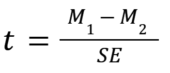
The most general formula for a t test is composed of two means (M1 and M2) and the overall standard error (SE) of the two samples:

See our video on How to Perform a Two-sample t test for an intuitive explanation of t tests and an example.

How to use the t test calculator

• Choose your data entry format . This will change how section 3 on the page looks. The first two options are for entering your data points themselves, either manually or by copy & paste. The last two are for entering the means for each group, along with the number of observations (N) and either the standard error of that mean (SEM) or standard deviation of the dataset (SD) standard error. If you have already calculated these summary statistics, the latter options will save you time.
• Choose a test from the three options: Unpaired t test, Welch's unpaired t test, or Paired t test. Use our Ultimate Guide to t tests if you are unsure which is appropriate, as it includes a section on "How do I know which t test to use?". Notice not all options are available if you enter means only.
• Enter data for the test, based on the format you chose in Step 1.
• Click Calculate Now and View the results. All options will perform a two-tailed test .

Performing t tests? We can help.

Sign up for more information on how to perform t tests and other common statistical analyses.

Common t test confusion

In addition to the number of t test options, t tests are often confused with completely different techniques as well. Here's how to keep them all straight.

Correlation and regression are used to measure how much two factors move together. While t tests are part of regression analysis, they are focused on only one factor by comparing means in different samples.

ANOVA is used for comparing means across three or more total groups. In contrast, t tests compare means between exactly two groups.

Finally, contingency tables compare counts of observations within groups rather than a calculated average. Since t tests compare means of continuous variable between groups, contingency tables use methods such as chi square instead of t tests.

Assumptions of t tests

Because there are several versions of t tests, it's important to check the assumptions to figure out which is best suited for your project. Here are our analysis checklists for unpaired t tests and paired t tests , which are the two most common. These (and the ultimate guide to t tests ) go into detail on the basic assumptions underlying any t test:

• Exactly two groups
• Sample is normally distributed
• Independent observations
• Unequal or equal variance?
• Paired or unpaired data?

Interpreting results

The three different options for t tests have slightly different interpretations, but they all hinge on hypothesis testing and P values. You need to select a significance threshold for your P value (often 0.05) before doing the test.

While P values can be easy to misinterpret , they are the most commonly used method to evaluate whether there is evidence of a difference between the sample of data collected and the null hypothesis. Once you have run the correct t test, look at the resulting P value. If the test result is less than your threshold, you have enough evidence to conclude that the data are significantly different.

If the test result is larger or equal to your threshold, you cannot conclude that there is a difference. However, you cannot conclude that there was definitively no difference either. It's possible that a dataset with more observations would have resulted in a different conclusion.

Depending on the test you run, you may see other statistics that were used to calculate the P value, including the mean difference, t statistic, degrees of freedom, and standard error. The confidence interval and a review of your dataset is given as well on the results page.

Graphing t tests

This calculator does not provide a chart or graph of t tests, however, graphing is an important part of analysis because it can help explain the results of the t test and highlight any potential outliers. See our Prism guide for some graphing tips for both unpaired and paired t tests.

Prism is built for customized, publication quality graphics and charts. For t tests we recommend simply plotting the datapoints themselves and the mean, or an estimation plot . Another popular approach is to use a violin plot, like those available in Prism.

For more information

Our ultimate guide to t tests includes examples, links, and intuitive explanations on the subject. It is quite simply the best place to start if you're looking for more about t tests!

If you enjoyed this calculator, you will love using Prism for analysis. Take a free 30-day trial to do more with your data, such as:

• Clear guidance to pick the right t test and detailed results summaries
• Custom, publication quality t test graphics, violin plots, and more
• More t test options, including normality testing as well as nested and multiple t tests
• Non-parametric test alternatives such as Wilcoxon, Mann-Whitney, and Kolmogorov-Smirnov

Check out our video on how to perform a t test in Prism , for an example from start to finish!

Remember, this page is just for two sample t tests. If you only have one sample, you need to use this calculator instead.

We Recommend:

Analyze, graph and present your scientific work easily with GraphPad Prism. No coding required.

• PRE-ALGEBRA
• MORE MATH FINANCE BUSINESS ENGINEERING FINANCE CHARTS MATH WORKSHEETS CURRENCY CONVERTER MULTIPLICATION TABLES DEPRECIATION SPORTS CALCULATORS HEALTH equations tricks history notes register login

• Engineering

t-Test Calculator

T-test - work with steps.

Input Data : Data set x = 3, 11, 17, 28, 34 Data set y = 5, 8, 13, 19, 28 Total number of elements = 5 Objective : Find the t-score by using mean and standard deviation. Solution : Mean 1 = (3 + 11 + 17 + 28 + 34)/5 = 93/5 Mean 1 = 18.6 Mean 2 = (5 + 8 + 13 + 19 + 28)/5 = 73/5 Mean 2 = 14.6 SD1 = √(1/5 - 1) x ((3 - 18.6) 2 + ( 11 - 18.6) 2 + ( 17 - 18.6) 2 + ( 28 - 18.6) 2 + ( 34 - 18.6) 2 ) = √(1/4) x ((-15.6) 2 + (-7.6) 2 + (-1.6) 2 + (9.4) 2 + (15.4) 2 ) = √(0.25) x ((243.36) + (57.76) + (2.56) + (88.36) + (237.16)) = √(0.25) x 629.2 = √157.3 SD1 = 12.5419 SD2 = √(1/5 - 1) x ((5 - 14.6) 2 + ( 8 - 14.6) 2 + ( 13 - 14.6) 2 + ( 19 - 14.6) 2 + ( 28 - 14.6) 2 ) = √(1/4) x ((-9.6) 2 + (-6.6) 2 + (-1.6) 2 + (4.4) 2 + (13.4) 2 ) = √(0.25) x ((92.16) + (43.56) + (2.56) + (19.36) + (179.56)) = √(0.25) x 337.2 = √84.3 SD2 = 9.1815 t-score = x 1 - x 2 √(SD1 2 /n1 + SD2 2 /n2) = 18.6 - 14.6 √((12.5419) 2 /5 + (9.1815) 2 /5) = 4 √((157.3)/5 + (84.3)/5) = 4 √(31.46 + 16.86) = 4 √(48.32) = 4 6.9513 t-score = 0.5754

t-test calculator is an online statistics tool to estimate the significance of observed differences between the means of two samples when there is a null hypothesis that is no significant difference between the means by using standard deviation. It is necessary to follow the next steps:

• Enter two samples (observed values) in the box. These values must be real numbers or variables and may be separated by commas. The values can be copied from a text document or a spreadsheet.
• Press the "GENERATE WORK" button to make the computation.
• t-Test calculator will give a test whether samples from two independent populations provide that the populations have different means.

What is t-Test?

A hypothesis test consists of two hypotheses, the null hypothesis and the alternative hypothesis or research hypothesis. The symbol $H_0$ represents the null hypothesis. The null hypothesis reflects that there will be no observed effect on the experiment. The null hypothesis consists of an equal sign. The alternative hypothesis reflects that there is an observed effect on the experiment. The symbol $H_a$ represents the alternative hypothesis. The first step in testing is to determine the null hypothesis and the alternative hypothesis. Regarding the testing hypothesis, there are some important terms. Rejection region is the set of values leads to rejection of the null hypothesis. Non-rejection region is the set of values that leads to nonrejection of the null hypothesis. Critical values are the value that separates the rejection and non-rejection regions. The t-Test is used in comparing the means of two populations. There are two approaches:

• When the samples from the two populations are independent;
• When the samples from the two populations are depended, i.e. when they are paired.
• If populations standard deviations are equal, $\sigma_1-\sigma_2$
• If populations standard deviations are different

How to Find t-Critical Value

To perform a hypothesis test to compare two population means, $\mu_1$ and $\mu_2$, we have some assumptions:

• Simple and independent random samples;
• Normal populations or large samples.

t-Test with Mean and Standard Deviation

A t-Test is one of the most frequently used tests in statistics. A t-Test is useful to conclude if the results are correct and applicable to the entire population. If we want to analyze simple experiments or when making simple comparisons between levels of independent variable we use the t-Test. It's used in comparison between two separate groups of individuals, for example: male vs female, experimental vs control group, etc. Practice Problem 1: There are two company A and B. We want to test average age of employees at these companies so we use a random sample of employee ages from each company.

• Hypergeometric distribution Calculator
• Error Function Calculator
• Beta Function Calculator
• Gamma Function Calculator
• Digamma Function Calculator
• F-Test Calculator
• Statistical Data Set Range Calculator
• Effect of Size Calculator
• Sampling Error Calculator
• Percent Error Calculator
• Percentile Calculator
• Signal to Noise Ratio Calculator

• Salary & Income Tax Calculators
• Mortgage Calculators
• Retirement Calculators
• Depreciation Calculators
• Statistics and Analysis Calculators
• Date and Time Calculators
• Contractor Calculators
• Budget & Savings Calculators
• Loan Calculators
• Forex Calculators
• Real Function Calculators
• Engineering Calculators
• Tax Calculators
• Volume Calculators
• 2D Shape Calculators
• 3D Shape Calculators
• Logistics Calculators
• HRM Calculators
• Sales & Investments Calculators
• Grade & GPA Calculators
• Conversion Calculators
• Ratio Calculators
• Sports & Health Calculators
• Other Calculators

Student T-Value Calculator

You can use this T-Value Calculator to calculate the Student's t-value based on the significance level and the degrees of freedom in the standard deviation.

How to use the calculator

• Enter the degrees of freedom (df)
• Enter the significance level alpha (α is a number between 0 and 1)
• Click the "Calculate" button to calculate the Student's t-critical value.

Degrees of Freedom (df) :

Significance Level (α) :

• Currently 4.76/5

Rating: 4.8 /5 (821 votes)

• Math Lessons
• Math Formulas
• Calculators

Math Calculators, Lessons and Formulas

It is time to solve your math problem

• HW Help (paid service)
• Statistics and probability
• T-test calculator

T-Test calculator

The Student's t-test is used to determine if means of two data sets differ significantly. This calculator will generate a step by step explanation on how to apply t - test.

• Factoring Polynomials
• Solving equations
• Rationalize Denominator
• Arithmetic sequences
• Polynomial Roots
• Synthetic Division
• Polynomial Operations
• Graphing Polynomials
• Simplify Polynomials
• Generate From Roots
• Simplify Expression
• Multiplication / Division
• Addition / Subtraction
• Simplifying
• Quadratic Equations Solver
• Polynomial Equations
• Solving Equations - With Steps
• Solving (with steps)
• Quadratic Plotter
• Factoring Trinomials
• Equilateral Triangle
• Right Triangle
• Oblique Triangle
• Square Calculator
• Rectangle Calculator
• Circle Calculator
• Hexagon Calculator
• Rhombus Calculator
• Trapezoid Calculator
• Triangular Prism
• Distance calculator
• Midpoint Calculator
• Triangle Calculator
• Graphing Lines
• Lines Intersection
• Two Point Form
• Line-Point Distance
• Parallel/Perpendicular
• Circle Equation
• Circle From 3 Points
• Circle-line Intersection
• Modulus, inverse, polar form
• Vectors (2D & 3D)
• Add, Subtract, Multiply
• Determinant Calculator
• Matrix Inverse
• Characteristic Polynomial
• Eigenvalues
• Eigenvectors
• Matrix Decomposition
• Limit Calculator
• Derivative Calculator
• Integral Calculator
• Arithmetic Sequences
• Geometric Sequences
• Find n th Term
• Degrees to Radians
• Trig. Equations
• Long Division
• Evaluate Expressions
• Fraction Calculator
• Greatest Common Divisor GCD
• Least Common Multiple LCM
• Prime Factorization
• Scientific Notation
• Percentage Calculator
• Dec / Bin / Hex
• Probability Calculator
• Probability Distributions
• Descriptive Statistics
• Standard Deviation
• Z - score Calculator
• Normal Distribution
• T-Test Calculator
• Correlation & Regression
• Simple Interest
• Compound Interest
• Amortization Calculator
• Annuity Calculator
• Work Problems

Hire MATHPORTAL experts to do math homework for you.

Prices start at $3 per problem.

Twelve younger adults and twelve older adults conducted a life satisfaction test. The data are presented in the table below. Compute the appropriate t-test.

Are the means between two data sets are significantly different at level $\alpha < 0.05$.

Related Calculators

Was this calculator helpful?

Please tell me how can I make this better.

Welcome to MathPortal. This website's owner is mathematician Miloš Petrović. I designed this website and wrote all the calculators, lessons, and formulas .

If you want to contact me, probably have some questions, write me using the contact form or email me on [email protected]

Email (optional)

P-value Calculator

Statistical significance calculator to easily calculate the p-value and determine whether the difference between two proportions or means (independent groups) is statistically significant. T-test calculator & z-test calculator to compute the Z-score or T-score for inference about absolute or relative difference (percentage change, percent effect). Suitable for analysis of simple A/B tests.

Related calculators

• Using the p-value calculator
• What is "p-value" and "significance level"
• P-value formula
• Why do we need a p-value?
• How to interpret a statistically significant result / low p-value
• P-value and significance for relative difference in means or proportions

    Using the p-value calculator

This statistical significance calculator allows you to perform a post-hoc statistical evaluation of a set of data when the outcome of interest is difference of two proportions (binomial data, e.g. conversion rate or event rate) or difference of two means (continuous data, e.g. height, weight, speed, time, revenue, etc.). You can use a Z-test (recommended) or a T-test to find the observed significance level (p-value statistic). The Student's T-test is recommended mostly for very small sample sizes, e.g. n < 30. In order to avoid type I error inflation which might occur with unequal variances the calculator automatically applies the Welch's T-test instead of Student's T-test if the sample sizes differ significantly or if one of them is less than 30 and the sampling ratio is different than one.

If entering proportions data, you need to know the sample sizes of the two groups as well as the number or rate of events. These can be entered as proportions (e.g. 0.10), percentages (e.g. 10%) or just raw numbers of events (e.g. 50).

If entering means data, simply copy/paste or type in the raw data, each observation separated by comma, space, new line or tab. Copy-pasting from a Google or Excel spreadsheet works fine.

The p-value calculator will output : p-value, significance level, T-score or Z-score (depending on the choice of statistical hypothesis test), degrees of freedom, and the observed difference. For means data it will also output the sample sizes, means, and pooled standard error of the mean. The p-value is for a one-sided hypothesis (one-tailed test), allowing you to infer the direction of the effect (more on one vs. two-tailed tests ). However, the probability value for the two-sided hypothesis (two-tailed p-value) is also calculated and displayed, although it should see little to no practical applications.

Warning: You must have fixed the sample size / stopping time of your experiment in advance, otherwise you will be guilty of optional stopping (fishing for significance) which will inflate the type I error of the test rendering the statistical significance level unusable. Also, you should not use this significance calculator for comparisons of more than two means or proportions, or for comparisons of two groups based on more than one metric. If a test involves more than one treatment group or more than one outcome variable you need a more advanced tool which corrects for multiple comparisons and multiple testing. This statistical calculator might help.

    What is "p-value" and "significance level"

The p-value is a heavily used test statistic that quantifies the uncertainty of a given measurement, usually as a part of an experiment, medical trial, as well as in observational studies. By definition, it is inseparable from inference through a Null-Hypothesis Statistical Test (NHST) . In it we pose a null hypothesis reflecting the currently established theory or a model of the world we don't want to dismiss without solid evidence (the tested hypothesis), and an alternative hypothesis: an alternative model of the world. For example, the statistical null hypothesis could be that exposure to ultraviolet light for prolonged periods of time has positive or neutral effects regarding developing skin cancer, while the alternative hypothesis can be that it has a negative effect on development of skin cancer.

In this framework a p-value is defined as the probability of observing the result which was observed, or a more extreme one, assuming the null hypothesis is true . In notation this is expressed as:

p(x 0 ) = Pr(d(X) > d(x 0 ); H 0 )

where x 0 is the observed data (x 1 ,x 2 ...x n ), d is a special function (statistic, e.g. calculating a Z-score), X is a random sample (X 1 ,X 2 ...X n ) from the sampling distribution of the null hypothesis. This equation is used in this p-value calculator and can be visualized as such:

Therefore the p-value expresses the probability of committing a type I error : rejecting the null hypothesis if it is in fact true. See below for a full proper interpretation of the p-value statistic .

Another way to think of the p-value is as a more user-friendly expression of how many standard deviations away from the normal a given observation is. For example, in a one-tailed test of significance for a normally-distributed variable like the difference of two means, a result which is 1.6448 standard deviations away (1.6448σ) results in a p-value of 0.05.

The term "statistical significance" or "significance level" is often used in conjunction to the p-value, either to say that a result is "statistically significant", which has a specific meaning in statistical inference ( see interpretation below ), or to refer to the percentage representation the level of significance: (1 - p value), e.g. a p-value of 0.05 is equivalent to significance level of 95% (1 - 0.05 * 100). A significance level can also be expressed as a T-score or Z-score, e.g. a result would be considered significant only if the Z-score is in the critical region above 1.96 (equivalent to a p-value of 0.025).

    P-value formula

There are different ways to arrive at a p-value depending on the assumption about the underlying distribution. This tool supports two such distributions: the Student's T-distribution and the normal Z-distribution (Gaussian) resulting in a T test and a Z test, respectively.

In both cases, to find the p-value start by estimating the variance and standard deviation, then derive the standard error of the mean, after which a standard score is found using the formula [2] :

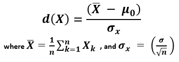
X (read "X bar") is the arithmetic mean of the population baseline or the control, μ 0 is the observed mean / treatment group mean, while σ x is the standard error of the mean (SEM, or standard deviation of the error of the mean).

When calculating a p-value using the Z-distribution the formula is Φ(Z) or Φ(-Z) for lower and upper-tailed tests, respectively. Φ is the standard normal cumulative distribution function and a Z-score is computed. In this mode the tool functions as a Z score calculator.

When using the T-distribution the formula is T n (Z) or T n (-Z) for lower and upper-tailed tests, respectively. T n is the cumulative distribution function for a T-distribution with n degrees of freedom and so a T-score is computed. Selecting this mode makes the tool behave as a T test calculator.

The population standard deviation is often unknown and is thus estimated from the samples, usually from the pooled samples variance. Knowing or estimating the standard deviation is a prerequisite for using a significance calculator. Note that differences in means or proportions are normally distributed according to the Central Limit Theorem (CLT) hence a Z-score is the relevant statistic for such a test.

    Why do we need a p-value?

If you are in the sciences, it is often a requirement by scientific journals. If you apply in business experiments (e.g. A/B testing) it is reported alongside confidence intervals and other estimates. However, what is the utility of p-values and by extension that of significance levels?

First, let us define the problem the p-value is intended to solve. People need to share information about the evidential strength of data that can be easily understood and easily compared between experiments. The picture below represents, albeit imperfectly, the results of two simple experiments, each ending up with the control with 10% event rate treatment group at 12% event rate.

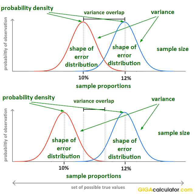
However, it is obvious that the evidential input of the data is not the same, demonstrating that communicating just the observed proportions or their difference (effect size) is not enough to estimate and communicate the evidential strength of the experiment. In order to fully describe the evidence and associated uncertainty , several statistics need to be communicated, for example, the sample size, sample proportions and the shape of the error distribution. Their interaction is not trivial to understand, so communicating them separately makes it very difficult for one to grasp what information is present in the data. What would you infer if told that the observed proportions are 0.1 and 0.12 (e.g. conversion rate of 10% and 12%), the sample sizes are 10,000 users each, and the error distribution is binomial?

Instead of communicating several statistics, a single statistic was developed that communicates all the necessary information in one piece: the p-value . A p-value was first derived in the late 18-th century by Pierre-Simon Laplace, when he observed data about a million births that showed an excess of boys, compared to girls. Using the calculation of significance he argued that the effect was real but unexplained at the time. We know this now to be true and there are several explanations for the phenomena coming from evolutionary biology. Statistical significance calculations were formally introduced in the early 20-th century by Pearson and popularized by Sir Ronald Fisher in his work, most notably "The Design of Experiments" (1935) [1] in which p-values were featured extensively. In business settings significance levels and p-values see widespread use in process control and various business experiments (such as online A/B tests, i.e. as part of conversion rate optimization, marketing optimization, etc.).

    How to interpret a statistically significant result / low p-value

Saying that a result is statistically significant means that the p-value is below the evidential threshold (significance level) decided for the statistical test before it was conducted. For example, if observing something which would only happen 1 out of 20 times if the null hypothesis is true is considered sufficient evidence to reject the null hypothesis, the threshold will be 0.05. In such case, observing a p-value of 0.025 would mean that the result is interpreted as statistically significant.

But what does that really mean? What inference can we make from seeing a result which was quite improbable if the null was true?

Observing any given low p-value can mean one of three things [3] :

• There is a true effect from the tested treatment or intervention.
• There is no true effect, but we happened to observe a rare outcome. The lower the p-value, the rarer (less likely, less probable) the outcome.
• The statistical model is invalid (does not reflect reality).

Obviously, one can't simply jump to conclusion 1.) and claim it with one hundred percent certainty, as this would go against the whole idea of the p-value and statistical significance. In order to use p-values as a part of a decision process external factors part of the experimental design process need to be considered which includes deciding on the significance level (threshold), sample size and power (power analysis), and the expected effect size, among other things. If you are happy going forward with this much (or this little) uncertainty as is indicated by the p-value calculation suggests, then you have some quantifiable guarantees related to the effect and future performance of whatever you are testing, e.g. the efficacy of a vaccine or the conversion rate of an online shopping cart.

Note that it is incorrect to state that a Z-score or a p-value obtained from any statistical significance calculator tells how likely it is that the observation is "due to chance" or conversely - how unlikely it is to observe such an outcome due to "chance alone". P-values are calculated under specified statistical models hence 'chance' can be used only in reference to that specific data generating mechanism and has a technical meaning quite different from the colloquial one. For a deeper take on the p-value meaning and interpretation, including common misinterpretations, see: definition and interpretation of the p-value in statistics .

    P-value and significance for relative difference in means or proportions

When comparing two independent groups and the variable of interest is the relative (a.k.a. relative change, relative difference, percent change, percentage difference), as opposed to the absolute difference between the two means or proportions, the standard deviation of the variable is different which compels a different way of calculating p-values [5] . The need for a different statistical test is due to the fact that in calculating relative difference involves performing an additional division by a random variable: the event rate of the control during the experiment which adds more variance to the estimation and the resulting statistical significance is usually higher (the result will be less statistically significant). What this means is that p-values from a statistical hypothesis test for absolute difference in means would nominally meet the significance level, but they will be inadequate given the statistical inference for the hypothesis at hand.

In simulations I performed the difference in p-values was about 50% of nominal: a 0.05 p-value for absolute difference corresponded to probability of about 0.075 of observing the relative difference corresponding to the observed absolute difference. Therefore, if you are using p-values calculated for absolute difference when making an inference about percentage difference, you are likely reporting error rates which are about 50% of the actual, thus significantly overstating the statistical significance of your results and underestimating the uncertainty attached to them.

In short - switching from absolute to relative difference requires a different statistical hypothesis test. With this calculator you can avoid the mistake of using the wrong test simply by indicating the inference you want to make.

    References

1 Fisher R.A. (1935) – "The Design of Experiments", Edinburgh: Oliver & Boyd

2 Mayo D.G., Spanos A. (2010) – "Error Statistics", in P. S. Bandyopadhyay & M. R. Forster (Eds.), Philosophy of Statistics, (7, 152–198). Handbook of the Philosophy of Science . The Netherlands: Elsevier.

3 Georgiev G.Z. (2017) "Statistical Significance in A/B Testing – a Complete Guide", [online] https://blog.analytics-toolkit.com/2017/statistical-significance-ab-testing-complete-guide/ (accessed Apr 27, 2018)

4 Mayo D.G., Spanos A. (2006) – "Severe Testing as a Basic Concept in a Neyman–Pearson Philosophy of Induction", British Society for the Philosophy of Science , 57:323-357

5 Georgiev G.Z. (2018) "Confidence Intervals & P-values for Percent Change / Relative Difference", [online] https://blog.analytics-toolkit.com/2018/confidence-intervals-p-values-percent-change-relative-difference/ (accessed May 20, 2018)

Cite this calculator & page

If you'd like to cite this online calculator resource and information as provided on the page, you can use the following citation: Georgiev G.Z., "P-value Calculator" , [online] Available at: https://www.gigacalculator.com/calculators/p-value-significance-calculator.php URL [Accessed Date: 16 May, 2024].

Our statistical calculators have been featured in scientific papers and articles published in high-profile science journals by:

The author of this tool

     Statistical calculators

• Student T-Value Calculator
• T Score vs Z Score
• Student T Test Excel
• T Table Calculator
• Student's T Test
• T Table Values
• Null Hypothesis T Test
• T Table Degrees of Freedom
• T Table Critical Values
• T Table Statistics
• Z Score Table
• T Table Confidence Interval
• T Table Hypothesis Testing
• Z Score Calculator
• Chi Square Table
• T Table Blog
• F Distribution Tables
• 1 mcg to mg
• 5 mcg to mg
• 10 mcg to mg
• 50 mcg to mg
• 100 mcg to mg
• 125 mcg to mg
• 200 mcg to mg
• 250 mcg to mg
• 300 mcg to mg
• 400 mcg to mg
• 500 mcg to mg
• 1000 mcg to mg
• 1 mg to mcg
• 2 mg to mcg
• 5 mg to cmg
• 10 mg to cmg
• 25 mg to mcg
• 50 mg to mcg
• 100 mg to mcg
• 200 mg to mcg
• 250 mg to mcg
• 1000 mg to mcg
• 1 tbsp to oz
• 2 tbsp to oz
• 3 tbsp to oz
• 4 tbsp to oz
• 5 tbsp to oz
• 6 tbsp to oz
• 1 tbsp to ml
• 2 tbsp to ml
• 3 tbsp to ml
• 5 tbsp to ml
• 0.5 KG to LB
• 1.7 KG to LB
• 10 KG to LB
• 15 KG to LB
• 20 KG to LB
• 22.5 KG to LB
• 23 KG to LB
• 25 KG to LB
• 50 KG to LB
• 60 KG to LB
• 65 KG to LB
• 70 KG to LB
• 80 KG to LB
• 90 KG to LB
• 100 KG to LB
• 150 KG to LB
• 60 LB to KG
• 90 LB to KG
• 120 LB to KG
• 130 LB to KG
• 135 LB to KG
• 140 LB to KG
• 150 LB to KG
• 155 LB to KG
• 160 LB to KG
• 165 LB to KG
• 170 LB to KG
• 180 LB to KG
• 190 LB to KG
• 200 LB to KG
• 160 CM to Feet
• 165 CM to Feet
• 168 CM to Feet
• 170 CM to Feet
• 172 CM to Feet
• 173 CM to Feet
• 175 CM to Feet
• 178 CM to Feet
• 180 CM to Feet
• 3 CM to Inches
• 5 CM to Inches
• 12 CM to Inches
• 13 CM to Inches
• 14 CM to Inches
• 15 CM to Inches
• 16 CM to Inches
• 17 CM to Inches
• 18 CM to Inches
• 20 CM to Inches
• 21 CM to Inches
• 22 CM to Inches
• 23 CM to Inches
• 25 CM to Inches
• 28 CM to Inches
• 30 CM to Inches
• 40 CM to Inches
• 45 CM to Inches
• 50 CM to Inches
• 60 CM to Inches
• 70 CM to Inches
• 90 CM to Inches
• 5 Inches to CM
• 6 Inches to CM
• 10 Inches to CM
• 12 Inches to CM
• 21 Inches to CM
• 23 Inches to CM
• 24 Inches to CM
• 28 Inches to CM
• 34 Inches to CM
• 35 Inches to CM
• 36 Inches to CM
• 43 Inches to CM
• 45 Inches to CM
• 54 Inches to CM
• 63 Inches to CM
• 71 Inches to CM
• 74 Inches to CM
• 96 Inches to CM
• 500 watts to amps
• 600 watts to amps
• 800 watts to amps
• 1000 watts to amps
• 1200 watts to amps
• 1500 watts to amps
• 2000 watts to amps
• 2500 watts to amps
• 3000 watts to amps
• 4000 watts to amps
• 5000 watts to amps
• 36.5 C to F
• 36.6 C to F
• 36.7 C to F
• 36.8 C to F
• 37.2 C to F
• 37.5 C to F
• 15 Fahrenheit to Celsius
• 40 Fahrenheit to Celsius
• 50 Fahrenheit to Celsius
• 60 Fahrenheit to Celsius
• 70 Fahrenheit to Celsius
• 72 Fahrenheit to Celsius
• 75 Fahrenheit to Celsius
• 80 Fahrenheit to Celsius
• 90 Fahrenheit to Celsius
• 100 Fahrenheit to Celsius
• 180 Fahrenheit to Celsius
• P Value Calculator
• I Roman Numerals
• II Roman Numerals
• III Roman Numerals
• IV Roman Numerals
• V Roman Numerals
• VI Roman Numerals
• VII Roman Numerals
• VIII Roman Numerals
• IX Roman Numerals
• X Roman Numerals
• XI Roman Numerals
• XII Roman Numerals
• XIII Roman Numerals
• XIV Roman Numerals
• XV Roman Numerals
• XVI Roman Numerals
• XVII Roman Numerals
• XVIII Roman Numerals
• XIX Roman Numerals
• XX Roman Numerals
• XXI Roman Numerals
• XXII Roman Numerals
• XXIII Roman Numerals
• XXIV Roman Numerals
• XXV Roman Numerals
• XXVI Roman Numerals
• XXVII Roman Numerals
• XXVIII Roman Numerals
• XXIX Roman Numerals
• XXX Roman Numerals
• XXXI Roman Numerals
• XXXII Roman Numerals
• XXXIII Roman Numerals
• XXXIV Roman Numerals
• XXXV Roman Numerals
• XXXVI Roman Numerals
• XXXVII Roman Numerals
• XXXVIII Roman Numerals
• XXXIX Roman Numerals
• XL Roman Numerals
• XLI Roman Numerals
• XLII Roman Numerals
• XLIII Roman Numerals
• XLIV Roman Numerals
• XLV Roman Numerals
• XLVI Roman Numerals
• XLVII Roman Numerals
• XLVIII Roman Numerals
• XLIX Roman Numerals
• L Roman Numerals
• LI Roman Numerals
• LII Roman Numerals
• LIII Roman Numerals
• LIV Roman Numerals
• LV Roman Numerals
• LVI Roman Numerals
• LVII Roman Numerals
• LVIII Roman Numerals
• LIX Roman Numerals
• LX Roman Numerals
• LXI Roman Numerals
• LXII Roman Numerals
• LXIII Roman Numerals
• LXIV Roman Numerals
• LXV Roman Numerals
• LXVI Roman Numerals
• LXVII Roman Numerals
• LXVIII Roman Numerals
• LXIX Roman Numerals
• LXX Roman Numerals
• LXXI Roman Numerals
• LXXII Roman Numerals
• LXXIII Roman Numerals
• LXXIV Roman Numerals
• LXXV Roman Numerals
• LXXVI Roman Numerals
• LXXVII Roman Numerals
• LXXVIII Roman Numerals
• LXXIX Roman Numerals
• LXXX Roman Numerals
• LXXXI Roman Numerals
• LXXXII Roman Numerals
• LXXXIII Roman Numerals
• LXXXIV Roman Numerals
• LXXXV Roman Numerals
• LXXXVI Roman Numerals
• LXXXVII Roman Numerals
• LXXXVIII Roman Numerals
• LXXXIX Roman Numerals
• XC Roman Numerals
• XCI Roman Numerals
• XCII Roman Numerals
• XCIII Roman Numerals
• XCIV Roman Numerals
• XCV Roman Numerals
• XCVI Roman Numerals
• XCVII Roman Numerals
• XCVIII Roman Numerals
• XCIX Roman Numerals
• C Roman Numerals
• CI Roman Numerals
• CII Roman Numerals
• CIII Roman Numerals
• CIV Roman Numerals
• CV Roman Numerals
• CVI Roman Numerals
• CVII Roman Numerals
• CVIII Roman Numerals
• CIX Roman Numerals
• CX Roman Numerals
• CXI Roman Numerals
• CXII Roman Numerals
• CXIII Roman Numerals
• CXIV Roman Numerals
• CXV Roman Numerals
• CXVI Roman Numerals
• CXVII Roman Numerals
• CXVIII Roman Numerals
• CXIX Roman Numerals
• CXX Roman Numerals
• CXXI Roman Numerals
• CXXII Roman Numerals
• CXXIII Roman Numerals
• CXXIV Roman Numerals
• CXXV Roman Numerals
• CXXVI Roman Numerals
• CXXVII Roman Numerals
• CXXVIII Roman Numerals
• CXXIX Roman Numerals
• CXXX Roman Numerals
• CXXXI Roman Numerals
• CXXXII Roman Numerals
• CXXXIII Roman Numerals
• CXXXIV Roman Numerals
• CXXXV Roman Numerals
• CXXXVI Roman Numerals
• CXXXVII Roman Numerals
• CXXXVIII Roman Numerals
• CXXXIX Roman Numerals
• CXL Roman Numerals
• CXLI Roman Numerals
• CXLII Roman Numerals
• CXLIII Roman Numerals
• CXLIV Roman Numerals
• CXLV Roman Numerals
• CXLVI Roman Numerals
• CXLVII Roman Numerals
• CXLVIII Roman Numerals
• CXLIX Roman Numerals
• CL Roman Numerals
• CLI Roman Numerals
• CLII Roman Numerals
• CLIII Roman Numerals
• CLIV Roman Numerals
• CLV Roman Numerals
• CLVI Roman Numerals
• CLVII Roman Numerals
• CLVIII Roman Numerals
• CLIX Roman Numerals
• CLX Roman Numerals
• CLXI Roman Numerals
• CLXII Roman Numerals
• CLXIII Roman Numerals
• CLXIV Roman Numerals
• Standard Deviation Calculator
• Using LETTERS in R: A Comprehensive Guide
• Combination Calculator
• Permutation Calculator
• Mean Calculator
• Median Calculator
• Empirical Rule Calculator
• Word Counter
• Factor Calculator
• Square Root Calculator
• Root Calculator
• Is 1 a Prime Number?
• Is 2 a Prime Number?
• Is 7 a Prime Number?
• Is 11 a Prime Number?
• Is 13 a Prime Number?
• Is 17 a Prime Number?
• Is 19 a Prime Number?
• Is 23 a Prime Number?
• Is 27 a Prime Number?
• Is 29 a Prime Number?
• Is 31 a Prime Number?
• Is 37 a Prime Number?
• Is 41 a Prime Number?
• Is 51 a Prime Number?
• Is 53 a Prime Number?
• Shoe Size EU to US
• Shoe Sizes Men to Women
• UK Shoe Size to US
• Online Timer
• Online Digital Stopwatch
• What are Mathematical Coordinates?

​Student t-Value Calculator Online

Student t-value calculator.

In order to calculate the Student T Value for any degrees of freedom and given probability. The calculator will return Student T Values for one tail (right) and two tailed probabilities. Please input degrees of freedom and probability level and then click “CALCULATE”

“extremely user friendly”

“truly amazing!”

“so easy to use!”

Statistics Calculator

You want to analyze your data effortlessly? DATAtab makes it easy and online.

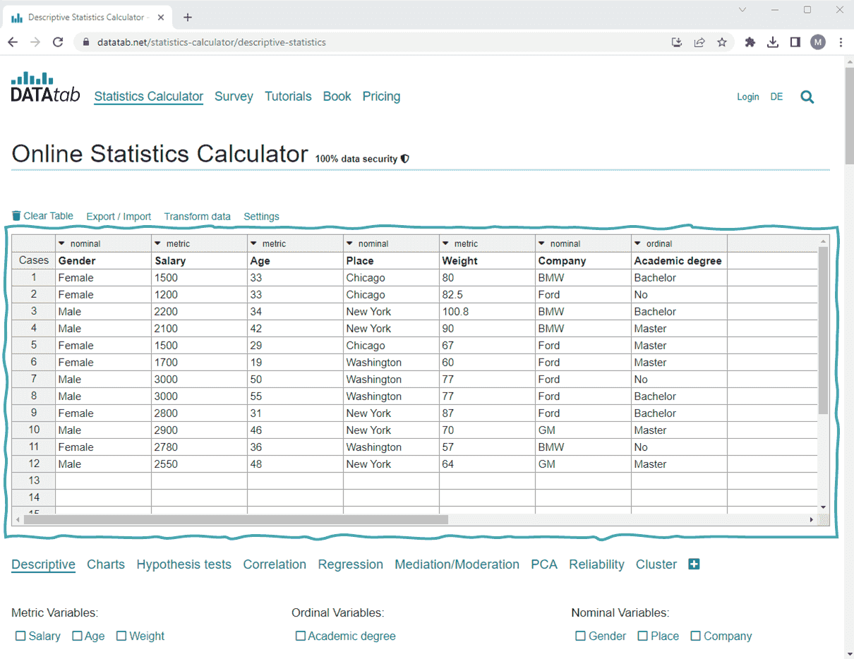
Online Statistics Calculator

What do you want to calculate online? The online statistics calculator is simple and uncomplicated! Here you can find a list of all implemented methods!

Create charts online with DATAtab

Create your charts for your data directly online and uncomplicated. To do this, insert your data into the table under Charts and select which chart you want.

The advantages of DATAtab

Statistics, as simple as never before..

DATAtab is a modern statistics software, with unique user-friendliness. Statistical analyses are done with just a few clicks, so DATAtab is perfect for statistics beginners and for professionals who want more flow in the user experience.

Directly in the browser, fully flexible.

Directly in the browser, fully flexible. DATAtab works directly in your web browser. You have no installation and maintenance effort whatsoever. Wherever and whenever you want to use DATAtab, just go to the website and get started.

All the statistical methods you need.

DATAtab offers you a wide range of statistical methods. We have selected the most central and best known statistical methods for you and do not overwhelm you with special cases.

Data security is a top priority.

All data that you insert and evaluate on DATAtab always remain on your end device. The data is not sent to any server or stored by us (not even temporarily). Furthermore, we do not pass on your data to third parties in order to analyze your user behavior.

Many tutorials with simple examples.

In order to facilitate the introduction, DATAtab offers a large number of free tutorials with focused explanations in simple language. We explain the statistical background of the methods and give step-by-step explanations for performing the analyses in the statistics calculator.

Practical Auto-Assistant.

DATAtab takes you by the hand in the world of statistics. When making statistical decisions, such as the choice of scale or measurement level or the selection of suitable methods, Auto-Assistants ensure that you get correct results quickly.

Charts, simple and clear.

With DATAtab data visualization is fun! Here you can easily create meaningful charts that optimally illustrate your results.

New in the world of statistics?

DATAtab was primarily designed for people for whom statistics is new territory. Beginners are not overwhelmed with a lot of complicated options and checkboxes, but are encouraged to perform their analyses step by step.

Online survey very simple.

DATAtab offers you the possibility to easily create an online survey, which you can then evaluate immediately with DATAtab.

Our references

Alternative to statistical software like SPSS and STATA

DATAtab was designed for ease of use and is a compelling alternative to statistical programs such as SPSS and STATA. On datatab.net, data can be statistically evaluated directly online and very easily (e.g. t-test, regression, correlation etc.). DATAtab's goal is to make the world of statistical data analysis as simple as possible, no installation and easy to use. Of course, we would also be pleased if you take a look at our second project Statisty .

Extensive tutorials

Descriptive statistics.

Here you can find out everything about location parameters and dispersion parameters and how you can describe and clearly present your data using characteristic values.

Hypothesis Test

Here you will find everything about hypothesis testing: One sample t-test , Unpaired t-test , Paired t-test and Chi-square test . You will also find tutorials for non-parametric statistical procedures such as the Mann-Whitney u-Test and Wilcoxon-Test . mann-whitney-u-test and the Wilcoxon test

The regression provides information about the influence of one or more independent variables on the dependent variable. Here are simple explanations of linear regression and logistic regression .

Correlation

Correlation analyses allow you to analyze the linear association between variables. Learn when to use Pearson correlation or Spearman rank correlation . With partial correlation , you can calculate the correlation between two variables to the exclusion of a third variable.

Partial Correlation

The partial correlation shows you the correlation between two variables to the exclusion of a third variable.

Levene Test

The Levene Test checks your data for variance equality. Thus, the levene test is used as a prerequisite test for many hypothesis tests .

The p-value is needed for every hypothesis test to be able to make a statement whether the null hypothesis is accepted or rejected.

Distributions

DATAtab provides you with tables with distributions and helpful explanations of the distribution functions. These include the Table of t-distribution and the Table of chi-squared distribution

Contingency table

With a contingency table you can get an overview of two categorical variables in the statistics.

Equivalence and non-inferiority

In an equivalence trial, the statistical test aims at showing that two treatments are not too different in characteristics and a non-inferiority trial wants to show that an experimental treatment is not worse than an established treatment.

If there is a clear cause-effect relationship between two variables, then we can speak of causality. Learn more about causality in our tutorial.

Multicollinearity

Multicollinearity is when two or more independent variables have a high correlation.

Effect size for independent t-test

Learn how to calculate the effect size for the t-test for independent samples.

Reliability analysis calculator

On DATAtab, Cohen's Kappa can be easily calculated online in the Cohen’s Kappa Calculator . there is also the Fleiss Kappa Calculator . Of course, the Cronbach's alpha can also be calculated in the Cronbach's Alpha Calculator .

Analysis of variance with repeated measurement

Repeated measures ANOVA tests whether there are statistically significant differences in three or more dependent samples.

Cite DATAtab: DATAtab Team (2024). DATAtab: Online Statistics Calculator. DATAtab e.U. Graz, Austria. URL https://datatab.net

Two Sample T-Test Calculator (Pooled-Variance)

Enter sample data, information, assumptions, required sample data.

• Calculators
• Descriptive Statistics
• Merchandise
• Which Statistics Test?

P Value from T Score Calculator

This should be self-explanatory, but just in case it's not: your t -score goes in the T Score box, you stick your degrees of freedom in the DF box ( N - 1 for single sample and dependent pairs, ( N 1 - 1 ) + ( N 2 - 1 ) for independent samples), select your significance level and whether you're testing a one or two-tailed hypothesis (if you're not sure, go with the defaults), then press the button.

If you need to derive a T Score from raw data, then you can find t test calculators here .

Enter your values above, then press "Calculate".

Additional T Statistic Calculators

If you're interested in using the t statistic for hypothesis testing and the like, then we have a number of other calculators that might help you.

T-Test Calculator for 2 Independent Means T-Test Calculator for 2 Dependent Means T-Test Calculator for a Single Sample

Statistics Made Easy

Two Sample t-test Calculator

t = -1.608761

p-value (one-tailed) = 0.060963

p-value (two-tailed) = 0.121926

Featured Posts

Hey there. My name is Zach Bobbitt. I have a Masters of Science degree in Applied Statistics and I’ve worked on machine learning algorithms for professional businesses in both healthcare and retail. I’m passionate about statistics, machine learning, and data visualization and I created Statology to be a resource for both students and teachers alike.  My goal with this site is to help you learn statistics through using simple terms, plenty of real-world examples, and helpful illustrations.

5 Replies to “Two Sample t-test Calculator”

Hi! Thanks for efforts.

-1.838687427 I get this for t value.

Could you please check? Classical two independant samples formula: t = (ma- mb)/ sqrt( s*s/12 – s*s/12)

Thank you learnt something. For df = 12, I had to subtract one from each of the samples

good work zach

Hi, I noticed that in using the calculators for hypothesis testing, the default level of significance is 0.05 and you cannot change it. Is there a way I can change the level of significance to 0.1 or say 0.01?

Leave a Reply Cancel reply

Your email address will not be published. Required fields are marked *

Join the Statology Community

Sign up to receive Statology's exclusive study resource: 100 practice problems with step-by-step solutions. Plus, get our latest insights, tutorials, and data analysis tips straight to your inbox!

By subscribing you accept Statology's Privacy Policy.

User Preferences

Content preview.

Arcu felis bibendum ut tristique et egestas quis:

• Ut enim ad minim veniam, quis nostrud exercitation ullamco laboris
• Duis aute irure dolor in reprehenderit in voluptate
• Excepteur sint occaecat cupidatat non proident

Keyboard Shortcuts

S.3.2 hypothesis testing (p-value approach).

The P -value approach involves determining "likely" or "unlikely" by determining the probability — assuming the null hypothesis was true — of observing a more extreme test statistic in the direction of the alternative hypothesis than the one observed. If the P -value is small, say less than (or equal to) \(\alpha\), then it is "unlikely." And, if the P -value is large, say more than \(\alpha\), then it is "likely."

If the P -value is less than (or equal to) \(\alpha\), then the null hypothesis is rejected in favor of the alternative hypothesis. And, if the P -value is greater than \(\alpha\), then the null hypothesis is not rejected.

Specifically, the four steps involved in using the P -value approach to conducting any hypothesis test are:

• Specify the null and alternative hypotheses.
• Using the sample data and assuming the null hypothesis is true, calculate the value of the test statistic. Again, to conduct the hypothesis test for the population mean μ , we use the t -statistic \(t^*=\frac{\bar{x}-\mu}{s/\sqrt{n}}\) which follows a t -distribution with n - 1 degrees of freedom.
• Using the known distribution of the test statistic, calculate the P -value : "If the null hypothesis is true, what is the probability that we'd observe a more extreme test statistic in the direction of the alternative hypothesis than we did?" (Note how this question is equivalent to the question answered in criminal trials: "If the defendant is innocent, what is the chance that we'd observe such extreme criminal evidence?")
• Set the significance level, \(\alpha\), the probability of making a Type I error to be small — 0.01, 0.05, or 0.10. Compare the P -value to \(\alpha\). If the P -value is less than (or equal to) \(\alpha\), reject the null hypothesis in favor of the alternative hypothesis. If the P -value is greater than \(\alpha\), do not reject the null hypothesis.

Example S.3.2.1

Mean gpa section  .

In our example concerning the mean grade point average, suppose that our random sample of n = 15 students majoring in mathematics yields a test statistic t * equaling 2.5. Since n = 15, our test statistic t * has n - 1 = 14 degrees of freedom. Also, suppose we set our significance level α at 0.05 so that we have only a 5% chance of making a Type I error.

Right Tailed

The P -value for conducting the right-tailed test H 0 : μ = 3 versus H A : μ > 3 is the probability that we would observe a test statistic greater than t * = 2.5 if the population mean \(\mu\) really were 3. Recall that probability equals the area under the probability curve. The P -value is therefore the area under a t n - 1 = t 14 curve and to the right of the test statistic t * = 2.5. It can be shown using statistical software that the P -value is 0.0127. The graph depicts this visually.

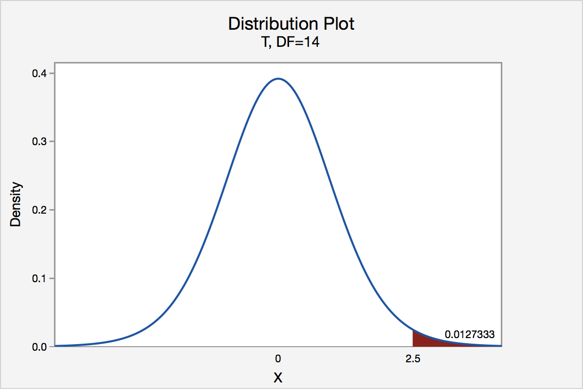
The P -value, 0.0127, tells us it is "unlikely" that we would observe such an extreme test statistic t * in the direction of H A if the null hypothesis were true. Therefore, our initial assumption that the null hypothesis is true must be incorrect. That is, since the P -value, 0.0127, is less than \(\alpha\) = 0.05, we reject the null hypothesis H 0 : μ = 3 in favor of the alternative hypothesis H A : μ > 3.

Note that we would not reject H 0 : μ = 3 in favor of H A : μ > 3 if we lowered our willingness to make a Type I error to \(\alpha\) = 0.01 instead, as the P -value, 0.0127, is then greater than \(\alpha\) = 0.01.

Left Tailed

In our example concerning the mean grade point average, suppose that our random sample of n = 15 students majoring in mathematics yields a test statistic t * instead of equaling -2.5. The P -value for conducting the left-tailed test H 0 : μ = 3 versus H A : μ < 3 is the probability that we would observe a test statistic less than t * = -2.5 if the population mean μ really were 3. The P -value is therefore the area under a t n - 1 = t 14 curve and to the left of the test statistic t* = -2.5. It can be shown using statistical software that the P -value is 0.0127. The graph depicts this visually.

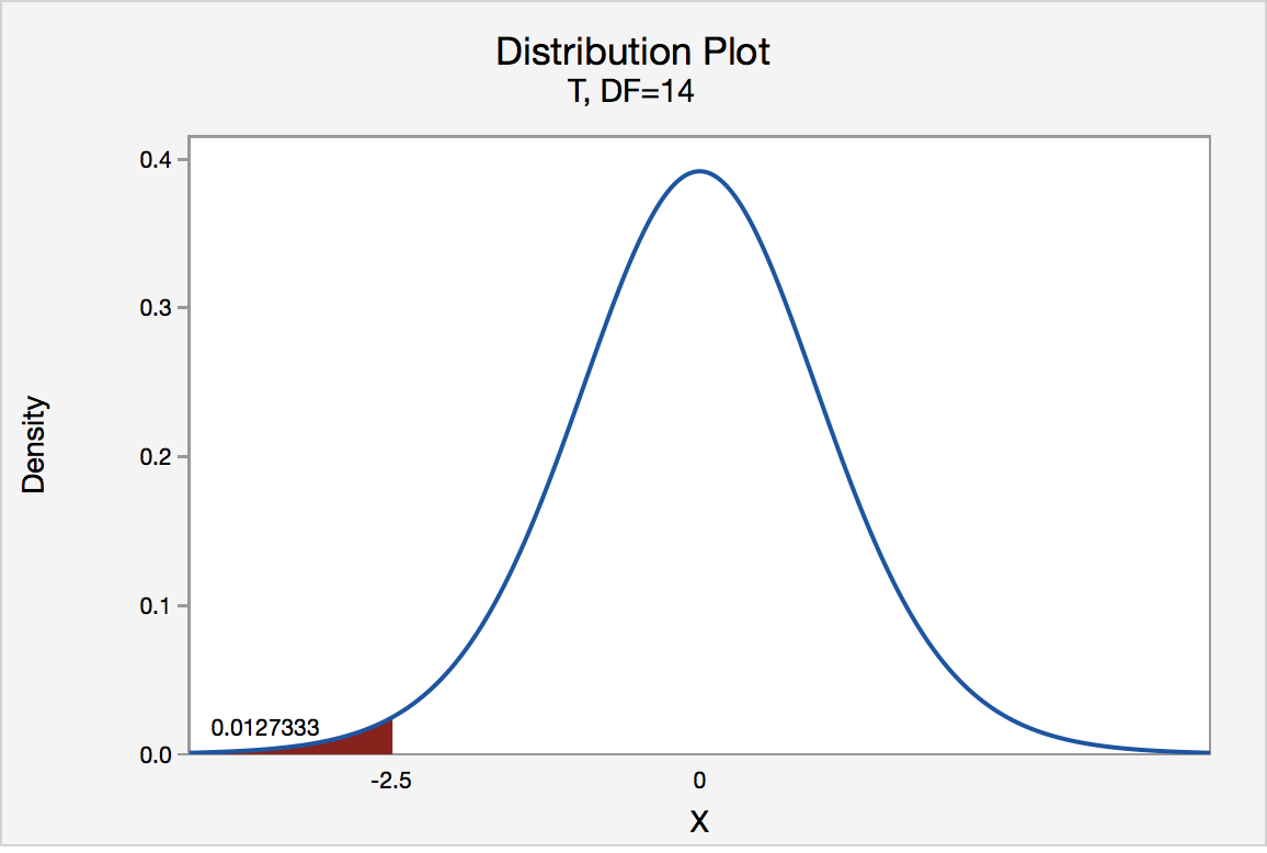
The P -value, 0.0127, tells us it is "unlikely" that we would observe such an extreme test statistic t * in the direction of H A if the null hypothesis were true. Therefore, our initial assumption that the null hypothesis is true must be incorrect. That is, since the P -value, 0.0127, is less than α = 0.05, we reject the null hypothesis H 0 : μ = 3 in favor of the alternative hypothesis H A : μ < 3.

Note that we would not reject H 0 : μ = 3 in favor of H A : μ < 3 if we lowered our willingness to make a Type I error to α = 0.01 instead, as the P -value, 0.0127, is then greater than \(\alpha\) = 0.01.

In our example concerning the mean grade point average, suppose again that our random sample of n = 15 students majoring in mathematics yields a test statistic t * instead of equaling -2.5. The P -value for conducting the two-tailed test H 0 : μ = 3 versus H A : μ ≠ 3 is the probability that we would observe a test statistic less than -2.5 or greater than 2.5 if the population mean μ really was 3. That is, the two-tailed test requires taking into account the possibility that the test statistic could fall into either tail (hence the name "two-tailed" test). The P -value is, therefore, the area under a t n - 1 = t 14 curve to the left of -2.5 and to the right of 2.5. It can be shown using statistical software that the P -value is 0.0127 + 0.0127, or 0.0254. The graph depicts this visually.

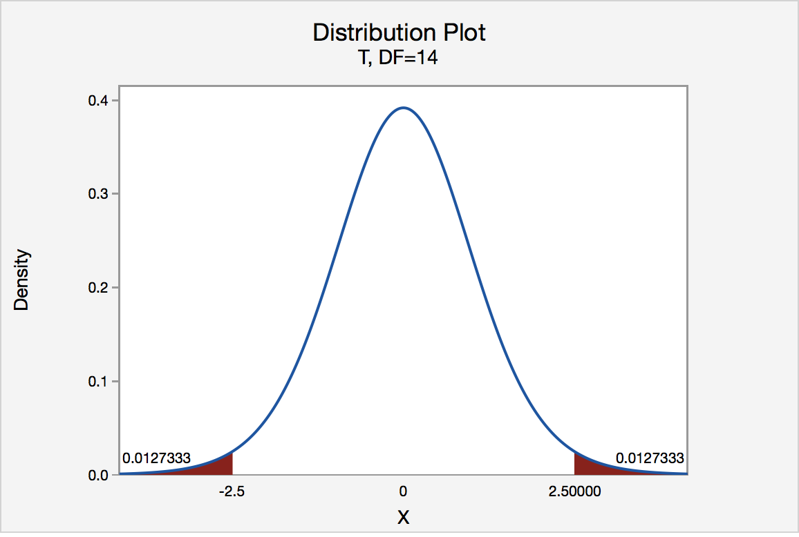
Note that the P -value for a two-tailed test is always two times the P -value for either of the one-tailed tests. The P -value, 0.0254, tells us it is "unlikely" that we would observe such an extreme test statistic t * in the direction of H A if the null hypothesis were true. Therefore, our initial assumption that the null hypothesis is true must be incorrect. That is, since the P -value, 0.0254, is less than α = 0.05, we reject the null hypothesis H 0 : μ = 3 in favor of the alternative hypothesis H A : μ ≠ 3.

Note that we would not reject H 0 : μ = 3 in favor of H A : μ ≠ 3 if we lowered our willingness to make a Type I error to α = 0.01 instead, as the P -value, 0.0254, is then greater than \(\alpha\) = 0.01.

Now that we have reviewed the critical value and P -value approach procedures for each of the three possible hypotheses, let's look at three new examples — one of a right-tailed test, one of a left-tailed test, and one of a two-tailed test.

The good news is that, whenever possible, we will take advantage of the test statistics and P -values reported in statistical software, such as Minitab, to conduct our hypothesis tests in this course.

How to Calculate p value from t test in Excel

Learn to calculate p-values in Excel for statistical significance. Explore methods, hypothesis testing roles & decision-making based... read more

#ez_toc_widget_sticky--1 .ez-toc-widget-sticky-container ul.ez-toc-widget-sticky-list li.active{ background-color: #ededed; } Steps To Follow

Get Trainings

Advance your Microsoft Excel & Office Skills with the MyExcelOnline Academy!

Peek through the statistical keyhole to discover the power of the P-value. It’s the probability that study results are due to chance if the null hypothesis holds true—essential for determining statistical significance. In this article, we will learn 2 quick methods on how to calculate p value in Microsoft Excel .

Key Takeaways:

• P-Value: The Statistical Key – It unveils the likelihood of chance influencing study outcomes if the null hypothesis were accurate.
• Data Preparation is Crucial – Before diving into P-value calculations, ensure your data is pristine, organized, and free from errors.
• Simple Methods for P-Value Calculation – Excel offers user-friendly functions like T.TEST and Data Analysis ToolPak for swift P-value determination.
• Interpreting P-Values – A P-value below 0.05 suggests significant findings, while above indicates results may be due to chance.

Table of Contents

Unlocking the Mystery of the P-Value in Excel

What is a p-value.

Imagine you’re peering through a keyhole at the secret workings of statistical analysis . Right there, in the center of it all, is the P-value—an intriguing figure that holds the power to unlock the truth behind your data. In statistics, the P-value represents the probability that the results of your study could occur by chance if the null hypothesis, which is usually a statement of ‘no effect’ or ‘no difference’, were true.

It’s essentially the key that statisticians use to determine whether or not they’ve stumbled upon something that could be statistically significant.

The Role of P-Value in Hypothesis Testing

When you’re delving into hypothesis testing, the P-value acts like a trusty sidekick, helping you to navigate the tricky terrain of statistical significance. Think of it as a guide that tells you whether the observational differences or relationships uncovered in your data are likely to hold true for the wider population, or if they might just be the result of random chance.

A smaller P-value, one that dips below the agreed-upon threshold (often 0.05), whispers a hint that your findings may challenge the status quo, suggesting that the null hypothesis might not hold up. On the flip side, a larger P-value, one that looms above this benchmark, suggests that the null hypothesis cannot be dismissed—the results could simply be a fluke of chance.

Setting the Stage for P-Value Calculation

Preparing your data for analysis.

Before you get to unravel the secrets of the P-value, it’s crucial that you set the stage right by preparing your data. This means you should start off by arranging your experimental results into two clean columns, each representing different conditions or groups for comparison. Make sure that your data is neatly formatted without any stray values that could throw off your calculations. Remove duplicates , correct any entry errors, and ensure that all data points are consistent in their units of measurement.

This meticulous preparation clears the path for a smoother analysis and more reliable insights, setting a rock-solid foundation for your P-value calculations.

The Roadmap to Calculating P-Value

Method 1: using the insert function button.

If you’re looking to calculate the P-value in Excel without getting too technical, then using the Insert Function button is like taking the scenic route on a data analysis road trip. Here’s what you need to do:

STEP 1: Park your cursor in the cell where you want the P-value to appear.

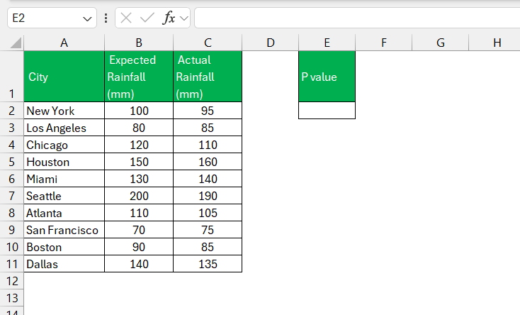
STEP 2: Click the “fx” button next to the formula bar, bringing up the Insert Function dialog box.

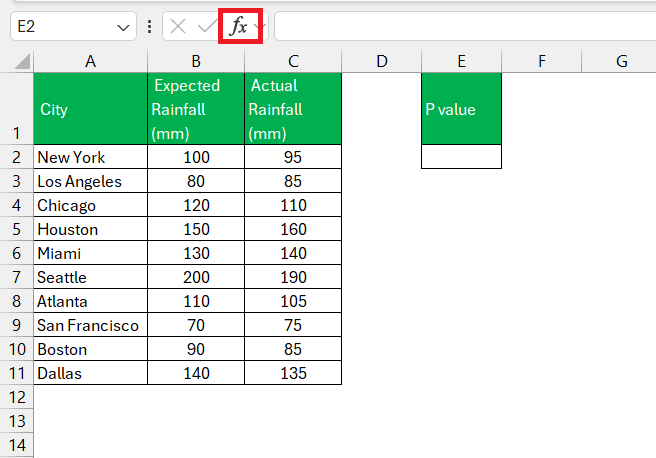
STEP 3: Now, type “T.TEST” into the search bar. When it pops up in the list, select it to open the door to calculate the P-value.

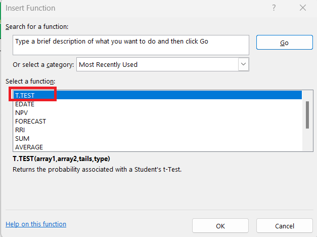
STEP 4: Next, you’ll be greeted by the Function Arguments dialog box. This is where you’ll input your data ranges for both groups you’re comparing into “Array1” and “Array2,” select whether you’re conducting a one-tailed or two-tailed test, and choose the type of t-test you’re running.

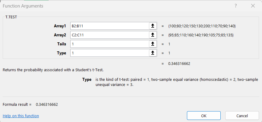
STEP 5: After hitting “OK,” Excel does the legwork and delivers the P-value right where you need it.

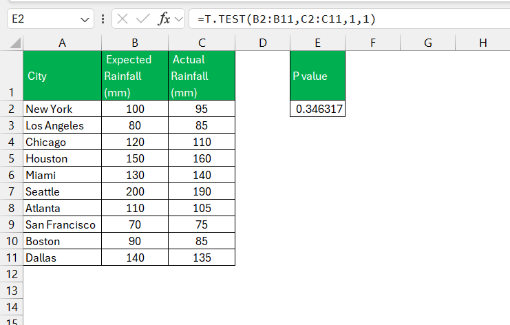
By using this friendly function, Excel handles the complex calculations in the background while you comfortably navigate through the intuitive interface.

Method 2: Delving into Analysis ToolPAk

To calculate the P-value using this method, follow the steps below:

STEP 1: Before we start, go to the Data Tab in Excel Ribbon and look for Data Analysis. If not found, follow the steps below to install it. Otherwise, you can directly go to STEP 5.

STEP 2: Go to File > Options.

STEP 3: In the dialog box, go to Add-ins in the left pane. Select Excel Add-ins from the dropdown and click on Go.

STEP 4: Select Analysis ToolPak and Click OK.

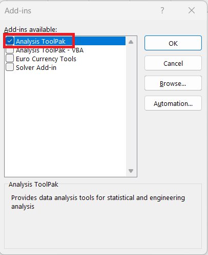
STEP 5: Go to Data Tab > Data Analysis.

STEP 6: In the Data Analysis dialog box, select ‘t-Test: Paired Two Sample for Means’ and click ‘OK’.

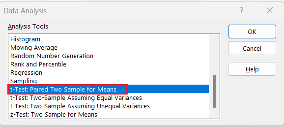
STEP 7: In the ‘t-Test: Paired Two Sample for Means’ dialogue box, select –

• Select the first data set as Variable Range 1.
• Select the second data set as Variable Range 2.
• Select Output Range.

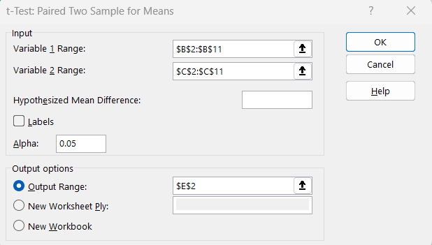
The p-value will be displayed in the t-test result.

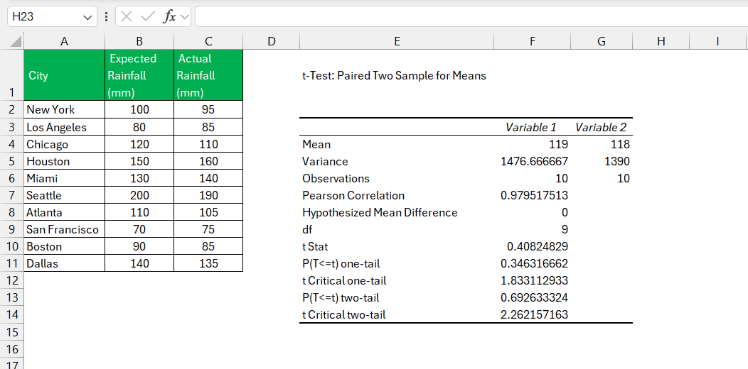
Specific Paths for Different Tests

Deciphering one-tailed p-value calculations.

Engage your statistical gears, because when you’re calculating a one-tailed P-value, you’re taking a more directed approach. You’re essentially investigating if one dataset is significantly greater than or less than the other, not just different. Excel simplifies this process through its functions, allowing you to focus on whether your data leans significantly in one direction.

As you unpack your one-tailed results, remember that a P-value greater than your alpha level (commonly set at 0.05) signals that you shouldn’t reject the null hypothesis. Your findings fall within the realm of normal range, with no significant slant. However, if your P-value cruises below that threshold, it’s waving a flag that the alternative hypothesis deserves some spotlight—that there’s a significant tilt in your data.

Navigating Through Two-Tailed P-Value Computations

Navigating through two-tailed P-value computations is like setting sail in open waters—you need to be prepared for anything, as you’re testing for any significant difference without specifying a direction. In Excel, achieving this balanced approach is a matter of adjusting your sails—simply replace the tails argument with 2 when using the T.TEST function or the T Distribution functions.

In this wider sea of possibilities, a small P-value, again compared against the alpha level of 0.05 or your chosen criterion, hints at the presence of a significant difference. But unlike a one-tailed test, direction doesn’t factor in. The key is the magnitude of the difference—whether one dataset is either much greater or much less—it’s the difference itself that’s significant here.

So batten down the hatches and make sure your data is shipshape. When done correctly, two-tailed tests provide a robust analysis of your datasets, ensuring you capture any significant differences, wherever they may lie.

Interpreting Your Results

What does your p-value mean.

Your P-value is like a secret message about your data waiting to be decoded. A small P-value, typically less than 0.05, is a whisper of a revelation—it hints strongly that your results might not be due to just luck or random chance, instead pointing to a real effect or difference. In contrast, a P-value that’s larger tells you to hold your horses—there’s not enough evidence to declare that what you’re observing is anything more than a statistical mirage.

Think of your P-value as a gauge on your dashboard, with 0.05 being a critical threshold. If the needle is to the left, switch on your “Eureka!” alert. To the right, and it’s time to keep the champagne on ice, as further investigation or new data might be necessary to draw firm conclusions.

Making Informed Decisions Based on P-Values

Making decisions based on P-values is akin to using a compass on a data-driven expedition. It doesn’t point you to an X-marks-the-spot treasure chest directly, but it helps you avoid wandering aimlessly or falling into the quicksand of faulty conclusions.

With a P-value in hand, you can make decisions with greater confidence. If the P-value sails below the 0.05 threshold, it’s a strong wind in your sails towards rejecting the null hypothesis and considering your alternative hypothesis credible. On the flip side, if the P-value is above 0.05, it’s wise to consider that your hypothesis might need revisiting, or that more data could be needed to clarify the waters.

However, it’s essential to weigh your P-value against the context of your study, including the effect size and confidence intervals. Sailing toward the truth involves considering all instruments at your disposal—not just the P-value compass.

FAQs on Calculating P-Value in Excel

What is p-value in excel.

The p-value in Excel is a probability score that tells you the strength of your evidence against the null hypothesis. It’s a way to measure if the data at hand could very well be a fluke or if there’s a statistically significant difference or association. In simpler terms, the p-value helps you understand whether your findings are due to actual effects or mere random chance.

How do you find the p-value in Excel?

To find the p-value in Excel, you’d typically use built-in functions like T.TEST for t-tests or the Data Analysis tool after installing the Analysis ToolPak. These Excel features help you calculate the p-value by inputting your data range, selecting tail type, and choosing the test type, guiding you swiftly towards the statistical significances in your data.

Is it necessary to have a strong statistics background to calculate p-values in Excel?

Not at all! While a solid grip on statistics can be beneficial, Excel’s user-friendly interface and functions greatly simplify the process of calculating p-values. You can perform these calculations effectively even with a basic understanding of statistical principles, thanks to Excel’s guided tools and wide array of resources available for support.

How can one-tailed and two-tailed tests affect the p-value in Excel?

In Excel, a one-tailed test evaluates if a dataset is significantly greater or less than another, influencing the p-value by focusing on a single direction of interest . Meanwhile, a two-tailed test checks for any significant difference regardless of direction, effectively doubling the critical area and can result in a larger p-value. Choosing between the two hinges on your hypothesis specifics, directly impacting the p-value and your conclusions.

Can Excel handle all types of hypothesis tests for p-value calculations?

Excel boasts a robust suite of statistical functions, able to tackle a wide range of hypothesis tests for p-value calculations. However, it may not be the best fit for extremely specialized or complex analyses, where dedicated statistical software would offer more nuanced control and options. For most standard tests, though, Excel has you covered.

John Michaloudis

John Michaloudis is a former accountant and finance analyst at General Electric, a Microsoft MVP since 2020, an Amazon #1 bestselling author of 4 Microsoft Excel books and teacher of Microsoft Excel & Office over at his flagship Academy Online Course .

Related Articles

How to Use Excel Rate Function for Interest Calculations

How to Graph Normal Distribution in Excel Fast

Excel Age Difference Calculator – How to Calculate Birthday Date & Gaps Fast!

Get Video Training

Dramatically Reduce Repetition, Stress, and Overtime! Exponentially Increase Your Chances of a Promotion, Pay Raise or New Job! Learn in as little as 5 minutes a day or on your schedule.