what dependent variable can be used to test the hypothesis

Want to create or adapt books like this? Learn more about how Pressbooks supports open publishing practices.

17 Introduction to Hypothesis Testing

Jenna Lehmann

What is Hypothesis Testing?

Hypothesis testing is a big part of what we would actually consider testing for inferential statistics. It’s a procedure and set of rules that allow us to move from descriptive statistics to make inferences about a population based on sample data. It is a statistical method that uses sample data to evaluate a hypothesis about a population.

This type of test is usually used within the context of research. If we expect to see a difference between a treated and untreated group (in some cases the untreated group is the parameters we know about the population), we expect there to be a difference in the means between the two groups, but that the standard deviation remains the same, as if each individual score has had a value added or subtracted from it.

Steps of Hypothesis Testing

The following steps will be tailored to fit the first kind of hypothesis testing we will learn first: single-sample z-tests. There are many other kinds of tests, so keep this in mind.

• Null Hypothesis (H0): states that in the general population there is no change, no difference, or no relationship, or in the context of an experiment, it predicts that the independent variable has no effect on the dependent variable.
• Alternative Hypothesis (H1): states that there is a change, a difference, or a relationship for the general population, or in the context of an experiment, it predicts that the independent variable has an effect on the dependent variable.

• Critical Region: Composed of the extreme sample values that are very unlikely to be obtained if the null hypothesis is true. Determined by alpha level. If sample data fall in the critical region, the null hypothesis is rejected, because it’s very unlikely they’ve fallen there by chance.
• After collecting the data, we find the sample mean. Now we can compare the sample mean with the null hypothesis by computing a z-score that describes where the sample mean is located relative to the hypothesized population mean. We use the z-score formula.
• We decided previously what the two z-score boundaries are for a critical score. If the z-score we get after plugging the numbers in the aforementioned equation is outside of that critical region, we reject the null hypothesis. Otherwise, we would say that we failed to reject the null hypothesis.

Regions of the Distribution

Because we’re making judgments based on probability and proportion, our normal distributions and certain regions within them come into play.

The Critical Region is composed of the extreme sample values that are very unlikely to be obtained if the null hypothesis is true. Determined by alpha level. If sample data fall in the critical region, the null hypothesis is rejected, because it’s very unlikely they’ve fallen there by chance.

These regions come into play when talking about different errors.

A Type I Error occurs when a researcher rejects a null hypothesis that is actually true; the researcher concludes that a treatment has an effect when it actually doesn’t. This happens when a researcher unknowingly obtains an extreme, non-representative sample. This goes back to alpha level: it’s the probability that the test will lead to a Type I error if the null hypothesis is true.

A result is said to be significant or statistically significant if it is very unlikely to occur when the null hypothesis is true. That is, the result is sufficient to reject the null hypothesis. For instance, two means can be significantly different from one another.

Factors that Influence and Assumptions of Hypothesis Testing

Assumptions of Hypothesis Testing:

• Random sampling: it is assumed that the participants used in the study were selected randomly so that we can confidently generalize our findings from the sample to the population.
• Independent observation: two observations are independent if there is no consistent, predictable relationship between the first observation and the second. The value of σ is unchanged by the treatment; if the population standard deviation is unknown, we assume that the standard deviation for the unknown population (after treatment) is the same as it was for the population before treatment. There are ways of checking to see if this is true in SPSS or Excel.
• Normal sampling distribution: in order to use the unit normal table to identify the critical region, we need the distribution of sample means to be normal (which means we need the population to be distributed normally and/or each sample size needs to be 30 or greater based on what we know about the central limit theorem).

Factors that influence hypothesis testing:

• The variability of the scores, which is measured by either the standard deviation or the variance. The variability influences the size of the standard error in the denominator of the z-score.
• The number of scores in the sample. This value also influences the size of the standard error in the denominator.

Test statistic: indicates that the sample data are converted into a single, specific statistic that is used to test the hypothesis (in this case, the z-score statistic).

Directional Hypotheses and Tailed Tests

In a directional hypothesis test , also known as a one-tailed test, the statistical hypotheses specify with an increase or decrease in the population mean. That is, they make a statement about the direction of the effect.

The Hypotheses for a Directional Test:

• H0: The test scores are not increased/decreased (the treatment doesn’t work)
• H1: The test scores are increased/decreased (the treatment works as predicted)

Because we’re only worried about scores that are either greater or less than the scores predicted by the null hypothesis, we only worry about what’s going on in one tail meaning that the critical region only exists within one tail. This means that all of the alpha is contained in one tail rather than split up into both (so the whole 5% is located in the tail we care about, rather than 2.5% in each tail). So before, we cared about what’s going on at the 0.025 mark of the unit normal table to look at both tails, but now we care about 0.05 because we’re only looking at one tail.

A one-tailed test allows you to reject the null hypothesis when the difference between the sample and the population is relatively small, as long as that difference is in the direction that you predicted. A two-tailed test, on the other hand, requires a relatively large difference independent of direction. In practice, researchers hypothesize using a one-tailed method but base their findings off of whether the results fall into the critical region of a two-tailed method. For the purposes of this class, make sure to calculate your results using the test that is specified in the problem.

Effect Size

A measure of effect size is intended to provide a measurement of the absolute magnitude of a treatment effect, independent of the size of the sample(s) being used. Usually done with Cohen’s d. If you imagine the two distributions, they’re layered over one another. The more they overlap, the smaller the effect size (the means of the two distributions are close). The more they are spread apart, the greater the effect size (the means of the two distributions are farther apart).

Statistical Power

The power of a statistical test is the probability that the test will correctly reject a false null hypothesis. It’s usually what we’re hoping to get when we run an experiment. It’s displayed in the table posted above. Power and effect size are connected. So, we know that the greater the distance between the means, the greater the effect size. If the two distributions overlapped very little, there would be a greater chance of selecting a sample that leads to rejecting the null hypothesis.

This chapter was originally posted to the Math Support Center blog at the University of Baltimore on June 11, 2019.

Math and Statistics Guides from UB's Math & Statistics Center Copyright © by Jenna Lehmann is licensed under a Creative Commons Attribution-NonCommercial-ShareAlike 4.0 International License , except where otherwise noted.

Share This Book

User Preferences

Content preview.

Arcu felis bibendum ut tristique et egestas quis:

• Ut enim ad minim veniam, quis nostrud exercitation ullamco laboris
• Duis aute irure dolor in reprehenderit in voluptate
• Excepteur sint occaecat cupidatat non proident

Keyboard Shortcuts

S.3 hypothesis testing.

In reviewing hypothesis tests, we start first with the general idea. Then, we keep returning to the basic procedures of hypothesis testing, each time adding a little more detail.

The general idea of hypothesis testing involves:

• Making an initial assumption.
• Collecting evidence (data).
• Based on the available evidence (data), deciding whether to reject or not reject the initial assumption.

Every hypothesis test — regardless of the population parameter involved — requires the above three steps.

Example S.3.1

Is normal body temperature really 98.6 degrees f section  .

Consider the population of many, many adults. A researcher hypothesized that the average adult body temperature is lower than the often-advertised 98.6 degrees F. That is, the researcher wants an answer to the question: "Is the average adult body temperature 98.6 degrees? Or is it lower?" To answer his research question, the researcher starts by assuming that the average adult body temperature was 98.6 degrees F.

Then, the researcher went out and tried to find evidence that refutes his initial assumption. In doing so, he selects a random sample of 130 adults. The average body temperature of the 130 sampled adults is 98.25 degrees.

Then, the researcher uses the data he collected to make a decision about his initial assumption. It is either likely or unlikely that the researcher would collect the evidence he did given his initial assumption that the average adult body temperature is 98.6 degrees:

• If it is likely , then the researcher does not reject his initial assumption that the average adult body temperature is 98.6 degrees. There is not enough evidence to do otherwise.
• either the researcher's initial assumption is correct and he experienced a very unusual event;
• or the researcher's initial assumption is incorrect.

In statistics, we generally don't make claims that require us to believe that a very unusual event happened. That is, in the practice of statistics, if the evidence (data) we collected is unlikely in light of the initial assumption, then we reject our initial assumption.

Example S.3.2

Criminal trial analogy section  .

One place where you can consistently see the general idea of hypothesis testing in action is in criminal trials held in the United States. Our criminal justice system assumes "the defendant is innocent until proven guilty." That is, our initial assumption is that the defendant is innocent.

In the practice of statistics, we make our initial assumption when we state our two competing hypotheses -- the null hypothesis ( H 0 ) and the alternative hypothesis ( H A ). Here, our hypotheses are:

• H 0 : Defendant is not guilty (innocent)
• H A : Defendant is guilty

In statistics, we always assume the null hypothesis is true . That is, the null hypothesis is always our initial assumption.

The prosecution team then collects evidence — such as finger prints, blood spots, hair samples, carpet fibers, shoe prints, ransom notes, and handwriting samples — with the hopes of finding "sufficient evidence" to make the assumption of innocence refutable.

In statistics, the data are the evidence.

The jury then makes a decision based on the available evidence:

• If the jury finds sufficient evidence — beyond a reasonable doubt — to make the assumption of innocence refutable, the jury rejects the null hypothesis and deems the defendant guilty. We behave as if the defendant is guilty.
• If there is insufficient evidence, then the jury does not reject the null hypothesis . We behave as if the defendant is innocent.

In statistics, we always make one of two decisions. We either "reject the null hypothesis" or we "fail to reject the null hypothesis."

Errors in Hypothesis Testing Section  

Did you notice the use of the phrase "behave as if" in the previous discussion? We "behave as if" the defendant is guilty; we do not "prove" that the defendant is guilty. And, we "behave as if" the defendant is innocent; we do not "prove" that the defendant is innocent.

This is a very important distinction! We make our decision based on evidence not on 100% guaranteed proof. Again:

• If we reject the null hypothesis, we do not prove that the alternative hypothesis is true.
• If we do not reject the null hypothesis, we do not prove that the null hypothesis is true.

We merely state that there is enough evidence to behave one way or the other. This is always true in statistics! Because of this, whatever the decision, there is always a chance that we made an error .

Let's review the two types of errors that can be made in criminal trials:

Table S.3.2 shows how this corresponds to the two types of errors in hypothesis testing.

Note that, in statistics, we call the two types of errors by two different  names -- one is called a "Type I error," and the other is called  a "Type II error." Here are the formal definitions of the two types of errors:

There is always a chance of making one of these errors. But, a good scientific study will minimize the chance of doing so!

Making the Decision Section  

Recall that it is either likely or unlikely that we would observe the evidence we did given our initial assumption. If it is likely , we do not reject the null hypothesis. If it is unlikely , then we reject the null hypothesis in favor of the alternative hypothesis. Effectively, then, making the decision reduces to determining "likely" or "unlikely."

In statistics, there are two ways to determine whether the evidence is likely or unlikely given the initial assumption:

• We could take the " critical value approach " (favored in many of the older textbooks).
• Or, we could take the " P -value approach " (what is used most often in research, journal articles, and statistical software).

In the next two sections, we review the procedures behind each of these two approaches. To make our review concrete, let's imagine that μ is the average grade point average of all American students who major in mathematics. We first review the critical value approach for conducting each of the following three hypothesis tests about the population mean $\mu$:

In Practice

• We would want to conduct the first hypothesis test if we were interested in concluding that the average grade point average of the group is more than 3.
• We would want to conduct the second hypothesis test if we were interested in concluding that the average grade point average of the group is less than 3.
• And, we would want to conduct the third hypothesis test if we were only interested in concluding that the average grade point average of the group differs from 3 (without caring whether it is more or less than 3).

Upon completing the review of the critical value approach, we review the P -value approach for conducting each of the above three hypothesis tests about the population mean \(\mu\). The procedures that we review here for both approaches easily extend to hypothesis tests about any other population parameter.

Statistics Resources

• Excel - Tutorials
• Basic Probability Rules
• Single Event Probability
• Complement Rule
• Intersections & Unions
• Compound Events
• Levels of Measurement
• Independent and Dependent Variables
• Entering Data
• Central Tendency
• Data and Tests
• Displaying Data
• Discussing Statistics In-text
• SEM and Confidence Intervals
• Two-Way Frequency Tables
• Empirical Rule
• Finding Probability
• Accessing SPSS
• Chart and Graphs
• Frequency Table and Distribution
• Descriptive Statistics
• Converting Raw Scores to Z-Scores
• Converting Z-scores to t-scores
• Split File/Split Output
• Partial Eta Squared
• Downloading and Installing G*Power: Windows/PC
• Correlation
• Testing Parametric Assumptions
• One-Way ANOVA
• Two-Way ANOVA
• Repeated Measures ANOVA
• Goodness-of-Fit
• Test of Association
• Pearson's r
• Point Biserial
• Mediation and Moderation
• Simple Linear Regression
• Multiple Linear Regression
• Binomial Logistic Regression
• Multinomial Logistic Regression
• Independent Samples T-test
• Dependent Samples T-test
• Testing Assumptions
• T-tests using SPSS
• T-Test Practice
• Predictive Analytics This link opens in a new window
• Quantitative Research Questions
• Null & Alternative Hypotheses
• One-Tail vs. Two-Tail
• Alpha & Beta
• Associated Probability
• Decision Rule
• Statement of Conclusion
• Statistics Group Sessions

ASC Chat Hours

ASC Chat is usually available at the following times ( Pacific Time):

If there is not a coach on duty, submit your question via one of the below methods:

  928-440-1325

  Ask a Coach

  [email protected]

Search our FAQs on the Academic Success Center's  Ask a Coach   page.

Reading List

In quantitative research, we can’t make claims without having some statistics to support it. In other words, it can’t be determined if the null or the alternative hypothesis is supported until the hypothesis has been explored, using the data that was collected.

There are numerous tests that can be used to test a hypothesis. Which test you use will depend on a number of factors. The purpose of this section is to discuss the basics of hypothesis testing.

Steps of Hypothesis Testing:

• State the Null & Alternative Hypotheses. These should reflect the hypothesis test that you anticipate conducting. For example, an alternative hypothesis for an ANOVA will state that there are significant differences between one or more means.
• Determine α. This refers to the amount of Type I error you are willing to make or the chance of determining that the null hypothesis is false when it is in fact true.
• State the decision rule. The decision rule states the circumstances under which the null hypothesis will be rejected. For a research paper, this will be comparing the obtained p-value (level of significance) of the test statistic to the alpha set for the hypothesis. For example, “If p < .05, the null hypothesis will be rejected.”
• Calculate the test statistic. In other words, conduct your hypothesis test with the appropriate statistical analysis. In most cases, this will be done using a statistical analysis tool, like SPSS.
• Reject the null hypothesis – In this case, the p-value for the test statistic is less than alpha. There is evidence to suggest the alternative is true.
• Fail to reject the null hypothesis – The p-value from the hypothesis test was greater than alpha. There is not sufficient evidence to suggest the null is not true.
• State the conclusion of the test in layman’s terms. This is where you connect the statistics back to the specific hypothesis being tested. For example, “The results of the hypothesis test indicate that the salary of factory workers varies based on gender.”

Was this resource helpful?

• << Previous: Quantitative Research Questions
• Next: Null & Alternative Hypotheses >>
• Last Updated: Apr 19, 2024 3:09 PM
• URL: https://resources.nu.edu/statsresources

Hypothesis testing

When interpreting research findings, researchers need to assess whether these findings may have occurred by chance. Hypothesis testing is a systematic procedure for deciding whether the results of a research study support a particular theory which applies to a population.

Hypothesis testing uses sample data to evaluate a hypothesis about a population . A hypothesis test assesses how unusual the result is, whether it is reasonable chance variation or whether the result is too extreme to be considered chance variation.

Basic concepts

• Null and research hypothesis

Probability value and types of errors

Effect size and statistical significance.

• Directional and non-directional hypotheses

Null and research hypotheses

To carry out statistical hypothesis testing, research and null hypothesis are employed:

• Research hypothesis : this is the hypothesis that you propose, also known as the alternative hypothesis HA. For example:

H A: There is a relationship between intelligence and academic results.

H A: First year university students obtain higher grades after an intensive Statistics course.

H A; Males and females differ in their levels of stress.

• The null hypothesis (H o ) is the opposite of the research hypothesis and expresses that there is no relationship between variables, or no differences between groups; for example:

H o : There is no relationship between intelligence and academic results.

H o:  First year university students do not obtain higher grades after an intensive Statistics course.

H o : Males and females will not differ in their levels of stress.

The purpose of hypothesis testing is to test whether the null hypothesis (there is no difference, no effect) can be rejected or approved. If the null hypothesis is rejected, then the research hypothesis can be accepted. If the null hypothesis is accepted, then the research hypothesis is rejected.

In hypothesis testing, a value is set to assess whether the null hypothesis is accepted or rejected and whether the result is statistically significant:

• A critical value is the score the sample would need to decide against the null hypothesis.
• A probability value is used to assess the significance of the statistical test. If the null hypothesis is rejected, then the alternative to the null hypothesis is accepted.

The probability value, or p value , is the probability of an outcome or research result given the hypothesis. Usually, the probability value is set at 0.05: the null hypothesis will be rejected if the probability value of the statistical test is less than 0.05. There are two types of errors associated to hypothesis testing:

• What if we observe a difference – but none exists in the population?
• What if we do not find a difference – but it does exist in the population?

These situations are known as Type I and Type II errors:

• Type I Error: is the type of error that involves the rejection of a null hypothesis that is actually true (i.e. a false positive).
• Type II Error:  is the type of error that occurs when we do not reject a null hypothesis that is false (i.e. a false negative).

These errors cannot be eliminated; they can be minimised, but minimising one type of error will increase the probability of committing the other type.

The probability of making a Type I error depends on the criterion that is used to accept or reject the null hypothesis: the p value or alpha level . The alpha is set by the researcher, usually at .05, and is the chance the researcher is willing to take and still claim the significance of the statistical test.). Choosing a smaller alpha level will decrease the likelihood of committing Type I error.

For example, p<0.05  indicates that there are 5 chances in 100 that the difference observed was really due to sampling error – that 5% of the time a Type I error will occur or that there is a 5% chance that the opposite of the null hypothesis is actually true.

With a p<0.01, there will be 1 chance in 100 that the difference observed was really due to sampling error – 1% of the time a Type I error will occur.

The p level is specified before analysing the data. If the data analysis results in a probability value below the α (alpha) level, then the null hypothesis is rejected; if it is not, then the null hypothesis is not rejected.

When the null hypothesis is rejected, the effect is said to be statistically significant. However, statistical significance does not mean that the effect is important.

A result can be statistically significant, but the effect size may be small. Finding that an effect is significant does not provide information about how large or important the effect is. In fact, a small effect can be statistically significant if the sample size is large enough.

Information about the effect size, or magnitude of the result, is given by the statistical test. For example, the strength of the correlation between two variables is given by the coefficient of correlation, which varies from 0 to 1.

• A hypothesis that states that students who attend an intensive Statistics course will obtain higher grades than students who do not attend would be directional.
• A non-directional hypothesis states that there will be differences between students who attend do or don’t attend an intensive Statistics course, but we don’t know what group will get higher grades than the other. The hypothesis only states that they will obtain different grades.

The hypothesis testing process

The hypothesis testing process can be divided into five steps:

• Restate the research question as research hypothesis and a null hypothesis about the populations.
• Determine the characteristics of the comparison distribution.
• Determine the cut off sample score on the comparison distribution at which the null hypothesis should be rejected.
• Determine your sample’s score on the comparison distribution.
• Decide whether to reject the null hypothesis.

This example illustrates how these five steps can be applied to text a hypothesis:

• Let’s say that you conduct an experiment to investigate whether students’ ability to memorise words improves after they have consumed caffeine.
• The experiment involves two groups of students: the first group consumes caffeine; the second group drinks water.
• Both groups complete a memory test.
• A randomly selected individual in the experimental condition (i.e. the group that consumes caffeine) has a score of 27 on the memory test. The scores of people in general on this memory measure are normally distributed with a mean of 19 and a standard deviation of 4.
• The researcher predicts an effect (differences in memory for these groups) but does not predict a particular direction of effect (i.e. which group will have higher scores on the memory test). Using the 5% significance level, what should you conclude?

Step 1 : There are two populations of interest.

Population 1: People who go through the experimental procedure (drink coffee).

Population 2: People who do not go through the experimental procedure (drink water).

• Research hypothesis: Population 1 will score differently from Population 2.
• Null hypothesis: There will be no difference between the two populations.

Step 2 : We know that the characteristics of the comparison distribution (student population) are:

Population M = 19, Population SD= 4, normally distributed. These are the mean and standard deviation of the distribution of scores on the memory test for the general student population.

Step 3 : For a two-tailed test (the direction of the effect is not specified) at the 5% level (25% at each tail), the cut off sample scores are +1.96 and -1.99.

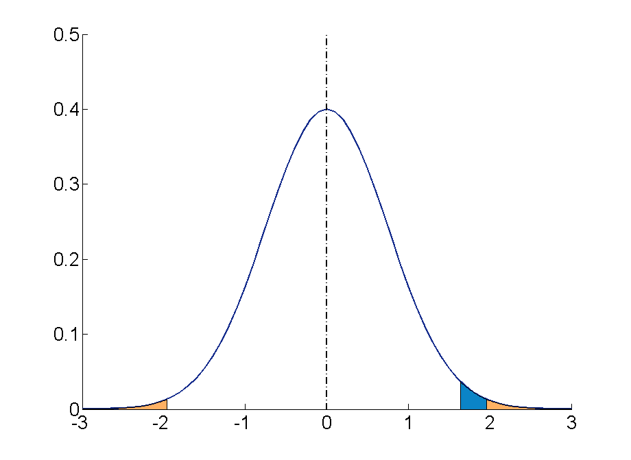
Step 4 : Your sample score of 27 needs to be converted into a Z value. To calculate Z = (27-19)/4= 2 ( check the Converting into Z scores section if you need to review how to do this process)

Step 5 : A ‘Z’ score of 2 is more extreme than the cut off Z of +1.96 (see figure above). The result is significant and, thus, the null hypothesis is rejected.

You can find more examples here:

• Statistics (RMIT Learning Lab)

Some commonly used statistical techniques

Correlation analysis, multiple regression.

• Analysis of variance

Chi-square test for independence

Correlation analysis explores the association between variables . The purpose of correlational analysis is to discover whether there is a relationship between variables, which is unlikely to occur by sampling error. The null hypothesis is that there is no relationship between the two variables. Correlation analysis provides information about:

• The direction of the relationship: positive or negative- given by the sign of the correlation coefficient.
• The strength or magnitude of the relationship between the two variables- given by the correlation coefficient, which varies from 0 (no relationship between the variables) to 1 (perfect relationship between the variables).
• Direction of the relationship.

A positive correlation indicates that high scores on one variable are associated with high scores on the other variable; low scores on one variable are associated with low scores on the second variable . For instance, in the figure below, higher scores on negative affect are associated with higher scores on perceived stress

A negative correlation indicates that high scores on one variable are associated with low scores on the other variable. The graph shows that a person who scores high on perceived stress will probably score low on mastery. The slope of the graph is downwards- as it moves to the right. In the figure below, higher scores on mastery are associated with lower scores on perceived stress.

Fig 2. Negative correlation between two variables. Adapted from Pallant, J. (2013). SPSS survival manual: A step by step guide to data analysis using IBM SPSS (5th ed.). Sydney, Melbourne, Auckland, London: Allen & Unwin

2. The strength or magnitude of the relationship

The strength of a linear relationship between two variables is measured by a statistic known as the correlation coefficient , which varies from 0 to -1, and from 0 to +1. There are several correlation coefficients; the most widely used are Pearson’s r and Spearman’s rho. The strength of the relationship is interpreted as follows:

• Small/weak: r= .10 to .29
• Medium/moderate: r= .30 to .49
• Large/strong: r= .50 to 1

It is important to note that correlation analysis does not imply causality. Correlation is used to explore the association between variables, however, it does not indicate that one variable causes the other. The correlation between two variables could be due to the fact that a third variable is affecting the two variables.

Multiple regression is an extension of correlation analysis. Multiple regression is used to explore the relationship between one dependent variable and a number of independent variables or predictors . The purpose of a multiple regression model is to predict values of a dependent variable based on the values of the independent variables or predictors. For example, a researcher may be interested in predicting students’ academic success (e.g. grades) based on a number of predictors, for example, hours spent studying, satisfaction with studies, relationships with peers and lecturers.

A multiple regression model can be conducted using statistical software (e.g. SPSS). The software will test the significance of the model (i.e. does the model significantly predicts scores on the dependent variable using the independent variables introduced in the model?), how much of the variance in the dependent variable is explained by the model, and the individual contribution of each independent variable.

Example of multiple regression model

From Dunn et al. (2014). Influence of academic self-regulation, critical thinking, and age on online graduate students' academic help-seeking.

In this model, help-seeking is the dependent variable; there are three independent variables or predictors. The coefficients show the direction (positive or negative) and magnitude of the relationship between each predictor and the dependent variable. The model was statistically significant and predicted 13.5% of the variance in help-seeking.

t-Tests are employed to compare the mean score on some continuous variable for two groups . The null hypothesis to be tested is there are no differences between the two groups (e.g. anxiety scores for males and females are not different).

If the significance value of the t-test is equal or less than .05, there is a significant difference in the mean scores on the variable of interest for each of the two groups. If the value is above .05, there is no significant difference between the groups.

t-Tests can be employed to compare the mean scores of two different groups (independent-samples t-test ) or to compare the same group of people on two different occasions ( paired-samples t-test) .

In addition to assessing whether the difference between the two groups is statistically significant, it is important to consider the effect size or magnitude of the difference between the groups. The effect size is given by partial eta squared (proportion of variance of the dependent variable that is explained by the independent variable) and Cohen’s d (difference between groups in terms of standard deviation units).

In this example, an independent samples t-test was conducted to assess whether males and females differ in their perceived anxiety levels. The significance of the test is .004. Since this value is less than .05, we can conclude that there is a statistically significant difference between males and females in their perceived anxiety levels.

Whilst t-tests compare the mean score on one variable for two groups, analysis of variance is used to test more than two groups . Following the previous example, analysis of variance would be employed to test whether there are differences in anxiety scores for students from different disciplines.

Analysis of variance compare the variance (variability in scores) between the different groups (believed to be due to the independent variable) with the variability within each group (believed to be due to chance). An F ratio is calculated; a large F ratio indicates that there is more variability between the groups (caused by the independent variable) than there is within each group (error term). A significant F test indicates that we can reject the null hypothesis; i.e. that there is no difference between the groups.

Again, effect size statistics such as Cohen’s d and eta squared are employed to assess the magnitude of the differences between groups.

In this example, we examined differences in perceived anxiety between students from different disciplines. The results of the Anova Test show that the significance level is .005. Since this value is below .05, we can conclude that there are statistically significant differences between students from different disciplines in their perceived anxiety levels.

Chi-square test for independence is used to explore the relationship between two categorical variables. Each variable can have two or more categories.

For example, a researcher can use a Chi-square test for independence to assess the relationship between study disciplines (e.g. Psychology, Business, Education,…) and help-seeking behaviour (Yes/No). The test compares the observed frequencies of cases with the values that would be expected if there was no association between the two variables of interest. A statistically significant Chi-square test indicates that the two variables are associated (e.g. Psychology students are more likely to seek help than Business students). The effect size is assessed using effect size statistics: Phi and Cramer’s V .

In this example, a Chi-square test was conducted to assess whether males and females differ in their help-seeking behaviour (Yes/No). The crosstabulation table shows the percentage of males of females who sought/didn't seek help. The table 'Chi square tests' shows the significance of the test (Pearson Chi square asymp sig: .482). Since this value is above .05, we conclude that there is no statistically significant difference between males and females in their help-seeking behaviour.

• << Previous: Probability and the normal distribution
• Next: Statistical techniques >>

Quantitative Analysis Guide: Choose Statistical Test for 2 or More Dependent Variables

• Finding Data
• Which Statistical Software to Use?
• Merging Data Sets
• Reshaping Data Sets
• Choose Statistical Test for 1 Dependent Variable
• Choose Statistical Test for 2 or More Dependent Variables

• Data Services Home Page
• Statistical Software Comparison
• What statistical test to use?
• Data Visualization Resources
• Data Analysis Examples External (UCLA) examples of regression and power analysis
• Supported software
• Request a consultation
• Making your code reproducible

Choosing a Statistical Test - Two or More Dependent Variables

• This table is designed to help you choose an appropriate statistical test for data with two or more dependent variables .
• Hover your mouse over the test name (in the Test column) to see its description.
• The Methodology column contains links to resources with more information about the test.
• The How To columns contain links with examples on how to run these tests in SPSS, Stata, SAS, R and MATLAB.
• The colors group statistical tests according to the key below:

* This is a user-written add-on

This page was adapted from the UCLA Statistical Consulting Group . We thank the UCLA Institute for Digital Research and Education (IDRE) for permission to adapt and distribute this page from our site.

• << Previous: Choose Statistical Test for 1 Dependent Variable
• Last Updated: Apr 18, 2024 4:36 AM
• URL: https://guides.nyu.edu/quant

Research Variables 101

Independent variables, dependent variables, control variables and more

By: Derek Jansen (MBA) | Expert Reviewed By: Kerryn Warren (PhD) | January 2023

If you’re new to the world of research, especially scientific research, you’re bound to run into the concept of variables , sooner or later. If you’re feeling a little confused, don’t worry – you’re not the only one! Independent variables, dependent variables, confounding variables – it’s a lot of jargon. In this post, we’ll unpack the terminology surrounding research variables using straightforward language and loads of examples .

Overview: Variables In Research

What (exactly) is a variable.

The simplest way to understand a variable is as any characteristic or attribute that can experience change or vary over time or context – hence the name “variable”. For example, the dosage of a particular medicine could be classified as a variable, as the amount can vary (i.e., a higher dose or a lower dose). Similarly, gender, age or ethnicity could be considered demographic variables, because each person varies in these respects.

Within research, especially scientific research, variables form the foundation of studies, as researchers are often interested in how one variable impacts another, and the relationships between different variables. For example:

• How someone’s age impacts their sleep quality
• How different teaching methods impact learning outcomes
• How diet impacts weight (gain or loss)

As you can see, variables are often used to explain relationships between different elements and phenomena. In scientific studies, especially experimental studies, the objective is often to understand the causal relationships between variables. In other words, the role of cause and effect between variables. This is achieved by manipulating certain variables while controlling others – and then observing the outcome. But, we’ll get into that a little later…

The “Big 3” Variables

Variables can be a little intimidating for new researchers because there are a wide variety of variables, and oftentimes, there are multiple labels for the same thing. To lay a firm foundation, we’ll first look at the three main types of variables, namely:

• Independent variables (IV)
• Dependant variables (DV)
• Control variables

What is an independent variable?

Simply put, the independent variable is the “ cause ” in the relationship between two (or more) variables. In other words, when the independent variable changes, it has an impact on another variable.

For example:

• Increasing the dosage of a medication (Variable A) could result in better (or worse) health outcomes for a patient (Variable B)
• Changing a teaching method (Variable A) could impact the test scores that students earn in a standardised test (Variable B)
• Varying one’s diet (Variable A) could result in weight loss or gain (Variable B).

It’s useful to know that independent variables can go by a few different names, including, explanatory variables (because they explain an event or outcome) and predictor variables (because they predict the value of another variable). Terminology aside though, the most important takeaway is that independent variables are assumed to be the “cause” in any cause-effect relationship. As you can imagine, these types of variables are of major interest to researchers, as many studies seek to understand the causal factors behind a phenomenon.

Need a helping hand?

What is a dependent variable?

While the independent variable is the “ cause ”, the dependent variable is the “ effect ” – or rather, the affected variable . In other words, the dependent variable is the variable that is assumed to change as a result of a change in the independent variable.

Keeping with the previous example, let’s look at some dependent variables in action:

• Health outcomes (DV) could be impacted by dosage changes of a medication (IV)
• Students’ scores (DV) could be impacted by teaching methods (IV)
• Weight gain or loss (DV) could be impacted by diet (IV)

In scientific studies, researchers will typically pay very close attention to the dependent variable (or variables), carefully measuring any changes in response to hypothesised independent variables. This can be tricky in practice, as it’s not always easy to reliably measure specific phenomena or outcomes – or to be certain that the actual cause of the change is in fact the independent variable.

As the adage goes, correlation is not causation . In other words, just because two variables have a relationship doesn’t mean that it’s a causal relationship – they may just happen to vary together. For example, you could find a correlation between the number of people who own a certain brand of car and the number of people who have a certain type of job. Just because the number of people who own that brand of car and the number of people who have that type of job is correlated, it doesn’t mean that owning that brand of car causes someone to have that type of job or vice versa. The correlation could, for example, be caused by another factor such as income level or age group, which would affect both car ownership and job type.

To confidently establish a causal relationship between an independent variable and a dependent variable (i.e., X causes Y), you’ll typically need an experimental design , where you have complete control over the environmen t and the variables of interest. But even so, this doesn’t always translate into the “real world”. Simply put, what happens in the lab sometimes stays in the lab!

As an alternative to pure experimental research, correlational or “ quasi-experimental ” research (where the researcher cannot manipulate or change variables) can be done on a much larger scale more easily, allowing one to understand specific relationships in the real world. These types of studies also assume some causality between independent and dependent variables, but it’s not always clear. So, if you go this route, you need to be cautious in terms of how you describe the impact and causality between variables and be sure to acknowledge any limitations in your own research.

What is a control variable?

In an experimental design, a control variable (or controlled variable) is a variable that is intentionally held constant to ensure it doesn’t have an influence on any other variables. As a result, this variable remains unchanged throughout the course of the study. In other words, it’s a variable that’s not allowed to vary – tough life 🙂

As we mentioned earlier, one of the major challenges in identifying and measuring causal relationships is that it’s difficult to isolate the impact of variables other than the independent variable. Simply put, there’s always a risk that there are factors beyond the ones you’re specifically looking at that might be impacting the results of your study. So, to minimise the risk of this, researchers will attempt (as best possible) to hold other variables constant . These factors are then considered control variables.

Some examples of variables that you may need to control include:

• Temperature
• Time of day
• Noise or distractions

Which specific variables need to be controlled for will vary tremendously depending on the research project at hand, so there’s no generic list of control variables to consult. As a researcher, you’ll need to think carefully about all the factors that could vary within your research context and then consider how you’ll go about controlling them. A good starting point is to look at previous studies similar to yours and pay close attention to which variables they controlled for.

Of course, you won’t always be able to control every possible variable, and so, in many cases, you’ll just have to acknowledge their potential impact and account for them in the conclusions you draw. Every study has its limitations, so don’t get fixated or discouraged by troublesome variables. Nevertheless, always think carefully about the factors beyond what you’re focusing on – don’t make assumptions!

Other types of variables

As we mentioned, independent, dependent and control variables are the most common variables you’ll come across in your research, but they’re certainly not the only ones you need to be aware of. Next, we’ll look at a few “secondary” variables that you need to keep in mind as you design your research.

• Moderating variables
• Mediating variables
• Confounding variables
• Latent variables

Let’s jump into it…

What is a moderating variable?

A moderating variable is a variable that influences the strength or direction of the relationship between an independent variable and a dependent variable. In other words, moderating variables affect how much (or how little) the IV affects the DV, or whether the IV has a positive or negative relationship with the DV (i.e., moves in the same or opposite direction).

For example, in a study about the effects of sleep deprivation on academic performance, gender could be used as a moderating variable to see if there are any differences in how men and women respond to a lack of sleep. In such a case, one may find that gender has an influence on how much students’ scores suffer when they’re deprived of sleep.

It’s important to note that while moderators can have an influence on outcomes , they don’t necessarily cause them ; rather they modify or “moderate” existing relationships between other variables. This means that it’s possible for two different groups with similar characteristics, but different levels of moderation, to experience very different results from the same experiment or study design.

What is a mediating variable?

Mediating variables are often used to explain the relationship between the independent and dependent variable (s). For example, if you were researching the effects of age on job satisfaction, then education level could be considered a mediating variable, as it may explain why older people have higher job satisfaction than younger people – they may have more experience or better qualifications, which lead to greater job satisfaction.

Mediating variables also help researchers understand how different factors interact with each other to influence outcomes. For instance, if you wanted to study the effect of stress on academic performance, then coping strategies might act as a mediating factor by influencing both stress levels and academic performance simultaneously. For example, students who use effective coping strategies might be less stressed but also perform better academically due to their improved mental state.

In addition, mediating variables can provide insight into causal relationships between two variables by helping researchers determine whether changes in one factor directly cause changes in another – or whether there is an indirect relationship between them mediated by some third factor(s). For instance, if you wanted to investigate the impact of parental involvement on student achievement, you would need to consider family dynamics as a potential mediator, since it could influence both parental involvement and student achievement simultaneously.

What is a confounding variable?

A confounding variable (also known as a third variable or lurking variable ) is an extraneous factor that can influence the relationship between two variables being studied. Specifically, for a variable to be considered a confounding variable, it needs to meet two criteria:

• It must be correlated with the independent variable (this can be causal or not)
• It must have a causal impact on the dependent variable (i.e., influence the DV)

Some common examples of confounding variables include demographic factors such as gender, ethnicity, socioeconomic status, age, education level, and health status. In addition to these, there are also environmental factors to consider. For example, air pollution could confound the impact of the variables of interest in a study investigating health outcomes.

Naturally, it’s important to identify as many confounding variables as possible when conducting your research, as they can heavily distort the results and lead you to draw incorrect conclusions . So, always think carefully about what factors may have a confounding effect on your variables of interest and try to manage these as best you can.

What is a latent variable?

Latent variables are unobservable factors that can influence the behaviour of individuals and explain certain outcomes within a study. They’re also known as hidden or underlying variables , and what makes them rather tricky is that they can’t be directly observed or measured . Instead, latent variables must be inferred from other observable data points such as responses to surveys or experiments.

For example, in a study of mental health, the variable “resilience” could be considered a latent variable. It can’t be directly measured , but it can be inferred from measures of mental health symptoms, stress, and coping mechanisms. The same applies to a lot of concepts we encounter every day – for example:

• Emotional intelligence
• Quality of life
• Business confidence
• Ease of use

One way in which we overcome the challenge of measuring the immeasurable is latent variable models (LVMs). An LVM is a type of statistical model that describes a relationship between observed variables and one or more unobserved (latent) variables. These models allow researchers to uncover patterns in their data which may not have been visible before, thanks to their complexity and interrelatedness with other variables. Those patterns can then inform hypotheses about cause-and-effect relationships among those same variables which were previously unknown prior to running the LVM. Powerful stuff, we say!

Let’s recap

In the world of scientific research, there’s no shortage of variable types, some of which have multiple names and some of which overlap with each other. In this post, we’ve covered some of the popular ones, but remember that this is not an exhaustive list .

To recap, we’ve explored:

• Independent variables (the “cause”)
• Dependent variables (the “effect”)
• Control variables (the variable that’s not allowed to vary)

If you’re still feeling a bit lost and need a helping hand with your research project, check out our 1-on-1 coaching service , where we guide you through each step of the research journey. Also, be sure to check out our free dissertation writing course and our collection of free, fully-editable chapter templates .

Psst... there’s more!

This post was based on one of our popular Research Bootcamps . If you're working on a research project, you'll definitely want to check this out ...

You Might Also Like:

Very informative, concise and helpful. Thank you

Helping information.Thanks

practical and well-demonstrated

Very helpful and insightful

Submit a Comment Cancel reply

Your email address will not be published. Required fields are marked *

Save my name, email, and website in this browser for the next time I comment.

• Print Friendly

Research Hypothesis In Psychology: Types, & Examples

Saul Mcleod, PhD

Editor-in-Chief for Simply Psychology

BSc (Hons) Psychology, MRes, PhD, University of Manchester

Saul Mcleod, PhD., is a qualified psychology teacher with over 18 years of experience in further and higher education. He has been published in peer-reviewed journals, including the Journal of Clinical Psychology.

Learn about our Editorial Process

Olivia Guy-Evans, MSc

Associate Editor for Simply Psychology

BSc (Hons) Psychology, MSc Psychology of Education

Olivia Guy-Evans is a writer and associate editor for Simply Psychology. She has previously worked in healthcare and educational sectors.

On This Page:

A research hypothesis, in its plural form “hypotheses,” is a specific, testable prediction about the anticipated results of a study, established at its outset. It is a key component of the scientific method .

Hypotheses connect theory to data and guide the research process towards expanding scientific understanding

Some key points about hypotheses:

• A hypothesis expresses an expected pattern or relationship. It connects the variables under investigation.
• It is stated in clear, precise terms before any data collection or analysis occurs. This makes the hypothesis testable.
• A hypothesis must be falsifiable. It should be possible, even if unlikely in practice, to collect data that disconfirms rather than supports the hypothesis.
• Hypotheses guide research. Scientists design studies to explicitly evaluate hypotheses about how nature works.
• For a hypothesis to be valid, it must be testable against empirical evidence. The evidence can then confirm or disprove the testable predictions.
• Hypotheses are informed by background knowledge and observation, but go beyond what is already known to propose an explanation of how or why something occurs.

Predictions typically arise from a thorough knowledge of the research literature, curiosity about real-world problems or implications, and integrating this to advance theory. They build on existing literature while providing new insight.

Types of Research Hypotheses

Alternative hypothesis.

The research hypothesis is often called the alternative or experimental hypothesis in experimental research.

It typically suggests a potential relationship between two key variables: the independent variable, which the researcher manipulates, and the dependent variable, which is measured based on those changes.

The alternative hypothesis states a relationship exists between the two variables being studied (one variable affects the other).

A hypothesis is a testable statement or prediction about the relationship between two or more variables. It is a key component of the scientific method. Some key points about hypotheses:

• Important hypotheses lead to predictions that can be tested empirically. The evidence can then confirm or disprove the testable predictions.

In summary, a hypothesis is a precise, testable statement of what researchers expect to happen in a study and why. Hypotheses connect theory to data and guide the research process towards expanding scientific understanding.

An experimental hypothesis predicts what change(s) will occur in the dependent variable when the independent variable is manipulated.

It states that the results are not due to chance and are significant in supporting the theory being investigated.

The alternative hypothesis can be directional, indicating a specific direction of the effect, or non-directional, suggesting a difference without specifying its nature. It’s what researchers aim to support or demonstrate through their study.

Null Hypothesis

The null hypothesis states no relationship exists between the two variables being studied (one variable does not affect the other). There will be no changes in the dependent variable due to manipulating the independent variable.

It states results are due to chance and are not significant in supporting the idea being investigated.

The null hypothesis, positing no effect or relationship, is a foundational contrast to the research hypothesis in scientific inquiry. It establishes a baseline for statistical testing, promoting objectivity by initiating research from a neutral stance.

Many statistical methods are tailored to test the null hypothesis, determining the likelihood of observed results if no true effect exists.

This dual-hypothesis approach provides clarity, ensuring that research intentions are explicit, and fosters consistency across scientific studies, enhancing the standardization and interpretability of research outcomes.

Nondirectional Hypothesis

A non-directional hypothesis, also known as a two-tailed hypothesis, predicts that there is a difference or relationship between two variables but does not specify the direction of this relationship.

It merely indicates that a change or effect will occur without predicting which group will have higher or lower values.

For example, “There is a difference in performance between Group A and Group B” is a non-directional hypothesis.

Directional Hypothesis

A directional (one-tailed) hypothesis predicts the nature of the effect of the independent variable on the dependent variable. It predicts in which direction the change will take place. (i.e., greater, smaller, less, more)

It specifies whether one variable is greater, lesser, or different from another, rather than just indicating that there’s a difference without specifying its nature.

For example, “Exercise increases weight loss” is a directional hypothesis.

Falsifiability

The Falsification Principle, proposed by Karl Popper , is a way of demarcating science from non-science. It suggests that for a theory or hypothesis to be considered scientific, it must be testable and irrefutable.

Falsifiability emphasizes that scientific claims shouldn’t just be confirmable but should also have the potential to be proven wrong.

It means that there should exist some potential evidence or experiment that could prove the proposition false.

However many confirming instances exist for a theory, it only takes one counter observation to falsify it. For example, the hypothesis that “all swans are white,” can be falsified by observing a black swan.

For Popper, science should attempt to disprove a theory rather than attempt to continually provide evidence to support a research hypothesis.

Can a Hypothesis be Proven?

Hypotheses make probabilistic predictions. They state the expected outcome if a particular relationship exists. However, a study result supporting a hypothesis does not definitively prove it is true.

All studies have limitations. There may be unknown confounding factors or issues that limit the certainty of conclusions. Additional studies may yield different results.

In science, hypotheses can realistically only be supported with some degree of confidence, not proven. The process of science is to incrementally accumulate evidence for and against hypothesized relationships in an ongoing pursuit of better models and explanations that best fit the empirical data. But hypotheses remain open to revision and rejection if that is where the evidence leads.

• Disproving a hypothesis is definitive. Solid disconfirmatory evidence will falsify a hypothesis and require altering or discarding it based on the evidence.
• However, confirming evidence is always open to revision. Other explanations may account for the same results, and additional or contradictory evidence may emerge over time.

We can never 100% prove the alternative hypothesis. Instead, we see if we can disprove, or reject the null hypothesis.

If we reject the null hypothesis, this doesn’t mean that our alternative hypothesis is correct but does support the alternative/experimental hypothesis.

Upon analysis of the results, an alternative hypothesis can be rejected or supported, but it can never be proven to be correct. We must avoid any reference to results proving a theory as this implies 100% certainty, and there is always a chance that evidence may exist which could refute a theory.

How to Write a Hypothesis

• Identify variables . The researcher manipulates the independent variable and the dependent variable is the measured outcome.
• Operationalized the variables being investigated . Operationalization of a hypothesis refers to the process of making the variables physically measurable or testable, e.g. if you are about to study aggression, you might count the number of punches given by participants.
• Decide on a direction for your prediction . If there is evidence in the literature to support a specific effect of the independent variable on the dependent variable, write a directional (one-tailed) hypothesis. If there are limited or ambiguous findings in the literature regarding the effect of the independent variable on the dependent variable, write a non-directional (two-tailed) hypothesis.
• Make it Testable : Ensure your hypothesis can be tested through experimentation or observation. It should be possible to prove it false (principle of falsifiability).
• Clear & concise language . A strong hypothesis is concise (typically one to two sentences long), and formulated using clear and straightforward language, ensuring it’s easily understood and testable.

Consider a hypothesis many teachers might subscribe to: students work better on Monday morning than on Friday afternoon (IV=Day, DV= Standard of work).

Now, if we decide to study this by giving the same group of students a lesson on a Monday morning and a Friday afternoon and then measuring their immediate recall of the material covered in each session, we would end up with the following:

• The alternative hypothesis states that students will recall significantly more information on a Monday morning than on a Friday afternoon.
• The null hypothesis states that there will be no significant difference in the amount recalled on a Monday morning compared to a Friday afternoon. Any difference will be due to chance or confounding factors.

More Examples

• Memory : Participants exposed to classical music during study sessions will recall more items from a list than those who studied in silence.
• Social Psychology : Individuals who frequently engage in social media use will report higher levels of perceived social isolation compared to those who use it infrequently.
• Developmental Psychology : Children who engage in regular imaginative play have better problem-solving skills than those who don’t.
• Clinical Psychology : Cognitive-behavioral therapy will be more effective in reducing symptoms of anxiety over a 6-month period compared to traditional talk therapy.
• Cognitive Psychology : Individuals who multitask between various electronic devices will have shorter attention spans on focused tasks than those who single-task.
• Health Psychology : Patients who practice mindfulness meditation will experience lower levels of chronic pain compared to those who don’t meditate.
• Organizational Psychology : Employees in open-plan offices will report higher levels of stress than those in private offices.
• Behavioral Psychology : Rats rewarded with food after pressing a lever will press it more frequently than rats who receive no reward.

• school Campus Bookshelves
• menu_book Bookshelves
• perm_media Learning Objects
• login Login
• how_to_reg Request Instructor Account
• hub Instructor Commons
• Download Page (PDF)
• Download Full Book (PDF)
• Periodic Table
• Physics Constants
• Scientific Calculator
• Reference & Cite
• Tools expand_more
• Readability

selected template will load here

This action is not available.

9.1: Two Sample Mean T-Test for Dependent Groups

• Last updated
• Save as PDF
• Page ID 24061

• Rachel Webb
• Portland State University

Dependent samples or matched pairs , occur when the subjects are paired up, or matched in some way. Most often, this model is characterized by selection of a random sample where each member is observed under two different conditions, before/after some experiment, or subjects that are similar (matched) to each other are studied under two different conditions.

There are 3 types of hypothesis tests for comparing two dependent population means µ 1 and µ 2 , where, µ D is the expected difference of the matched pairs.

Note: If each pair were equal to one another then the mean of the differences would be zero. We could also use this model to test with a magnitude of a difference, but we rarely cover that scenario, therefore we are usually test against the difference of zero.

The t-test for dependent samples is a statistical test for comparing the means from two dependent populations (or the difference between the means from two populations). The t-test is used when the differences are normally distributed. The samples also must be dependent.

The formula for the t-test statistic is: \(t=\frac{\bar{D}-\mu_{D}}{\left(\frac{S_{D}}{\sqrt{n}}\right)}\).

Where the t-distribution with degrees of freedom, df = n – 1

Note we will usually only use the case where µ D equals zero.

The subscript “ D ” denotes the difference between population one and two. It is important to compute D = x 1 – x 2 for each pair of observations. However, this makes setting up the hypotheses more challenging for one-tailed tests.

If we were looking for an increase in test scores from before to after, then we would expect the after score to be larger. When we take a smaller number minus a larger number then the difference would be negative. If we put the before group first and the after group second then we would need a left-tailed test μ D < 0 to test the “increase” in test scores. This is opposite of the sign we associate for “increase.” If we swap the order and use the after group first, then the before group would have a larger number minus a smaller number which would be positive and we would do a right-tailed test μ D > 0.

Always subtract in the same order the data is presented in the question. An easier way to decide on the one-tailed test is to write down the two labels and then put a less than () symbol between them depending on the question. For example, if the research statement is a weight loss program significantly decreases the average weight, the sign of the test would change depending on which group came first. If we subtract before weight – after weight, then we would want to have before > after and use μ D > 0. If we have the after weight as the first measurement then we would subtract the after weight – before weight and want after < before and use μ D < 0. If you keep your labels in the same order as they appear in the question, compare them and carry this sign down to the alternative hypothesis.

The traditional method (or critical value method), the p-value method, and the confidence interval method are performed with steps that are identical to those when performing hypothesis tests for one population.

A dietician is testing to see if a new diet program reduces the average weight. They randomly sample 35 patients and measure them before they start the program and then weigh them again after 2 months on the program. What are the correct hypotheses?

Let x 1 = weight before a weight-loss program and x 2 = weight after the weight-loss program. We want to test if, on average, participants lose weight. Therefore, the difference D = x 1 – x 2 . This gives D = before weight – after weight, thus if on average people do lose weight, then in general the before > after and the D’s are positive. How we define our differences determines that this example is a right-tailed test (carry the > sign down to the alternative hypothesis) and the correct hypotheses are:

H 0 : µ D = 0

H 1 : µ D > 0

If we were to do the same problem but reverse the order and take D = after weight – before weight the correct alternative hypothesis is H 1 : µ D < 0 since after weight < before weight. Just be consistent throughout your problem, and never switch the order of the groups in a problem.

P-Value Method Example

In an effort to increase production of an automobile part, the factory manager decides to play music in the manufacturing area. Eight workers are selected, and the number of items each produced for a specific day is recorded. After one week of music, the same workers are monitored again. The data are given in the table. At \(\alpha\) = 0.05, can the manager conclude that the music has increased production? Assume production is normally distributed. Use the p-value method.

Using the 1-var stats on the differences in your calculator, we compute \(\bar{D}=\bar{x}=2\), s D = s x = 2.0702, n = 8.

The test statistic is: \(\t=\frac{\bar{D}-\mu_{D}}{\left(\frac{s_{D}}{\sqrt{n}}\right)}=\frac{-2-0}{\left(\frac{2.0702}{\sqrt{8}}\right)}=-2.7325\).

The p-value for a two-tailed t-test with degrees of freedom = n – 1 = 7, is found by finding the area to the left of the test statistic –2.7325 using technology.

Decision: Since the p-value = 0.0146 is less than \(\alpha\) = 0.05, we reject H 0 .

Summary: At the 5% level of significance, there is enough evidence to support the claim that the mean production rate increases when music is played in the manufacturing area.

TI-84: Find the differences between the sample pairs (you can subtract two lists to do this). Press the [STAT] key and then the [EDIT] function, enter the difference column into list one. Press the [STAT] key, arrow over to the [TESTS] menu. Arrow down to the option [2:T -Test] and press the [ENTER]. Arrow over to the [Data] menu and press the [ENTER] key. Then type in the hypothesized mean as 0, List: L3, leave Freq:1 alone, arrow over to the \(\neq\), <, >, sign that is the same in the problem’s alternative hypothesis statement then press the [ENTER] key, arrow down to [Calculate] and press the [ENTER] key. The calculator returns the t-test statistic, the p-value, mean of the differences \(\bar{D}=\bar{x}\) and standard deviation of the differences s D = s x .

TI-89: Find the differences between the sample pairs (you can subtract two lists to do this). Go to the [Apps] Stat/List Editor , enter the two data sets in lists 1 and 2. Move the cursor so that it is highlighted on the header of list3. Press [2 nd ] Var-Link and move down to list1 and press [Enter]. This brings the name list1 back to the list3 at the bottom, select the minus [-] key, then select [2 nd ] Var-link and this time highlight list2 and press [Enter]. You should now see list1-list2 at the bottom of the window. Press [Enter] then the differences will be stored in list3. Press [2 nd ] then F6 [Tests], select 2: T-Test . Select the [Data] menu. Then type in the hypothesized mean as 0, List: list1, Freq:1, arrow over to the \(\neq\), <, >, and select the sign that is the same in the problem’s alternative hypothesis, press the [ENTER] key to calculate. The calculator returns the t-test statistic, p-value, \(\bar{D}=\bar{x}\) and s D = s x .

Excel: Start by entering the data in two columns in the same order that they appear in the problem. Then select Data > Data Analysis > t-test: Paired Two Sample for Means, then select OK.

Select the Before data (including the label) into the Variable 1 Range, and the After data (including the label) in the Variable 2 Range. Type in zero for the Hypothesized Mean Difference box. Select the box for Labels (do not select this if you do not have labels in the variable range selected). Change alpha to fit the problem. You can leave the default to open in a new worksheet or change output range to be one cell where you want the top left of the output table to start (make sure this cell does not overlap any existing data). Then select OK. See below for example.

You get the following output:

One nice feature in Excel is that you get the p-value and the critical value in the output. The critical value can be taken from the Excel output; however, Excel never gives negative critical values. Since we are doing a left-tailed test we will need to use the t-score = -1.8946.

If we were to draw and shade the critical region for the sampling distribution, it would look like Figure 9 -2.

The decision is made by comparing the test statistic t = -2.7325 with the critical value t α = -1.8946.

Since the test statistic is in the shaded critical region, we would reject H 0 .

At the 5% level of significance, there is enough evidence to support the claim that the mean production rate increases when music is played in the manufacturing area.

The decision and summary should not change from using the p-value method.

Confidence Interval Method

A (1 – \(\alpha\))*100% confidence interval for the difference between two population means with matched pairs: μ D = mean of the differences.

\(\bar{D}-t_{\frac{\alpha}{2}}\left(\frac{s_{D}}{\sqrt{n}}\right)<\mu_{D}<\bar{D}+t_{\alpha / 2}\left(\frac{s_{D}}{\sqrt{n}}\right)\]

Or more compactly as \(\bar{D} \pm t_{\alpha / 2}\left(\frac{s_{D}}{\sqrt{n}}\right)\)

Where the t-distribution has degrees of freedom, df = n – 1, where n is the number of pairs.

Hands-On Cafe records the number of online orders for eight randomly selected locations for two consecutive days. Assume the number of online orders is normally distributed. Find the 95% confidence interval for the mean difference. Is there evidence of a difference in mean number of orders for the two days?

Use technology to compute the mean, standard deviation and sample size.

Note if you use a TI calculator then \(\bar{D}=\bar{x}\) and s D = s x .

Find the interval estimate: \(\bar{D} \pm t_{\frac{\alpha}{2}}\left(\frac{s_{D}}{\sqrt{n}}\right)\)

\(\begin{aligned} &\Rightarrow-1.75 \pm 2.36462\left(\frac{2.05287}{\sqrt{8}}\right) \\ &\Rightarrow-1.75 \pm 1.7162 . \end{aligned}\)

Write the answer using standard notation –3.4662 < μ D < –0.0335 or interval notation (–3.4662, –0.0338).

For an interpretation of the interval, if we were to use the same sampling techniques, approximately 95 out of 100 times the confidence interval (–3.4662, –0.0338) would contain the population mean difference in the number of orders between Thursday and Friday.

Since both endpoints are negative, we can be 95% confident that the population mean number of orders for Thursday is between 3.4662 and 0.0338 orders lower than Friday.

Excel: Type in both samples in two adjacent columns, and then subtract each pair in a third column and label the column Difference.

Select Data > Data Analysis > Descriptive Statistics and click OK.

Select the Difference column for the input range including the label, then check the box next to Labels in first row (do not select this box if you did not highlight a label in the input range). Use the default new worksheet or select a single cell for the Output Range where you want your top left-hand corner of the table to start. Check the boxes Summary Statistics and Confidence Level for Mean. Change the confidence level to fit the question, and then select OK.

The confidence interval is the mean ± margin of error. In two different cells subtract and then add the margin of error from the mean to get the confidence interval limits and then put your answer in interval notation (–3.4662, – 0.0338).

TI-84: First, find the differences between the samples. Then on the TI-83 press the [STAT] key, arrow over to the [TESTS] menu, arrow down to the [8:TInterval] option and press the [ENTER] key. Arrow over to the [Data] menu and press the [ENTER] key. The defaults are List: L1, Freq:1. If this is set with a different list, arrow down and use [2 nd ] [1] to get L1. Then type in the confidence level. Arrow down to [Calculate] and press the [ENTER] key. The calculator returns the confidence interval, \(\bar{D}=\bar{x}\) and s D = s x .

TI-89: First, find the differences between the samples. Go to the [Apps] Stat/List Editor , then enter the differences into list 1. Press [2 nd ] then F7 [Ints], then select 2: T-Interval . Select the [Data] menu. Enter in List: list1, Freq:1. Then type in the confidence level. Press the [ENTER] key to calculate. The calculator returns the confidence interval, \(\bar{D}=\bar{x}\) and s D = s x .

• Bipolar Disorder
• Therapy Center
• When To See a Therapist
• Types of Therapy
• Best Online Therapy
• Best Couples Therapy
• Best Family Therapy
• Managing Stress
• Sleep and Dreaming
• Understanding Emotions
• Self-Improvement
• Healthy Relationships
• Student Resources
• Personality Types
• Guided Meditations
• Verywell Mind Insights
• 2023 Verywell Mind 25
• Mental Health in the Classroom
• Editorial Process
• Meet Our Review Board
• Crisis Support

How to Write a Great Hypothesis

Hypothesis Definition, Format, Examples, and Tips

Kendra Cherry, MS, is a psychosocial rehabilitation specialist, psychology educator, and author of the "Everything Psychology Book."

Amy Morin, LCSW, is a psychotherapist and international bestselling author. Her books, including "13 Things Mentally Strong People Don't Do," have been translated into more than 40 languages. Her TEDx talk,  "The Secret of Becoming Mentally Strong," is one of the most viewed talks of all time.

Verywell / Alex Dos Diaz

• The Scientific Method

Hypothesis Format

Falsifiability of a hypothesis.

• Operationalization

Hypothesis Types

Hypotheses examples.

• Collecting Data

A hypothesis is a tentative statement about the relationship between two or more variables. It is a specific, testable prediction about what you expect to happen in a study. It is a preliminary answer to your question that helps guide the research process.

Consider a study designed to examine the relationship between sleep deprivation and test performance. The hypothesis might be: "This study is designed to assess the hypothesis that sleep-deprived people will perform worse on a test than individuals who are not sleep-deprived."

At a Glance

A hypothesis is crucial to scientific research because it offers a clear direction for what the researchers are looking to find. This allows them to design experiments to test their predictions and add to our scientific knowledge about the world. This article explores how a hypothesis is used in psychology research, how to write a good hypothesis, and the different types of hypotheses you might use.

The Hypothesis in the Scientific Method

In the scientific method , whether it involves research in psychology, biology, or some other area, a hypothesis represents what the researchers think will happen in an experiment. The scientific method involves the following steps:

• Forming a question
• Performing background research
• Creating a hypothesis
• Designing an experiment
• Collecting data
• Analyzing the results
• Drawing conclusions
• Communicating the results

The hypothesis is a prediction, but it involves more than a guess. Most of the time, the hypothesis begins with a question which is then explored through background research. At this point, researchers then begin to develop a testable hypothesis.

Unless you are creating an exploratory study, your hypothesis should always explain what you  expect  to happen.

In a study exploring the effects of a particular drug, the hypothesis might be that researchers expect the drug to have some type of effect on the symptoms of a specific illness. In psychology, the hypothesis might focus on how a certain aspect of the environment might influence a particular behavior.

Remember, a hypothesis does not have to be correct. While the hypothesis predicts what the researchers expect to see, the goal of the research is to determine whether this guess is right or wrong. When conducting an experiment, researchers might explore numerous factors to determine which ones might contribute to the ultimate outcome.

In many cases, researchers may find that the results of an experiment  do not  support the original hypothesis. When writing up these results, the researchers might suggest other options that should be explored in future studies.

In many cases, researchers might draw a hypothesis from a specific theory or build on previous research. For example, prior research has shown that stress can impact the immune system. So a researcher might hypothesize: "People with high-stress levels will be more likely to contract a common cold after being exposed to the virus than people who have low-stress levels."

In other instances, researchers might look at commonly held beliefs or folk wisdom. "Birds of a feather flock together" is one example of folk adage that a psychologist might try to investigate. The researcher might pose a specific hypothesis that "People tend to select romantic partners who are similar to them in interests and educational level."

Elements of a Good Hypothesis

So how do you write a good hypothesis? When trying to come up with a hypothesis for your research or experiments, ask yourself the following questions:

• Is your hypothesis based on your research on a topic?
• Can your hypothesis be tested?
• Does your hypothesis include independent and dependent variables?

Before you come up with a specific hypothesis, spend some time doing background research. Once you have completed a literature review, start thinking about potential questions you still have. Pay attention to the discussion section in the  journal articles you read . Many authors will suggest questions that still need to be explored.

How to Formulate a Good Hypothesis

To form a hypothesis, you should take these steps:

• Collect as many observations about a topic or problem as you can.
• Evaluate these observations and look for possible causes of the problem.
• Create a list of possible explanations that you might want to explore.
• After you have developed some possible hypotheses, think of ways that you could confirm or disprove each hypothesis through experimentation. This is known as falsifiability.

In the scientific method ,  falsifiability is an important part of any valid hypothesis. In order to test a claim scientifically, it must be possible that the claim could be proven false.

Students sometimes confuse the idea of falsifiability with the idea that it means that something is false, which is not the case. What falsifiability means is that  if  something was false, then it is possible to demonstrate that it is false.

One of the hallmarks of pseudoscience is that it makes claims that cannot be refuted or proven false.

The Importance of Operational Definitions

A variable is a factor or element that can be changed and manipulated in ways that are observable and measurable. However, the researcher must also define how the variable will be manipulated and measured in the study.

Operational definitions are specific definitions for all relevant factors in a study. This process helps make vague or ambiguous concepts detailed and measurable.

For example, a researcher might operationally define the variable " test anxiety " as the results of a self-report measure of anxiety experienced during an exam. A "study habits" variable might be defined by the amount of studying that actually occurs as measured by time.

These precise descriptions are important because many things can be measured in various ways. Clearly defining these variables and how they are measured helps ensure that other researchers can replicate your results.

Replicability

One of the basic principles of any type of scientific research is that the results must be replicable.

Replication means repeating an experiment in the same way to produce the same results. By clearly detailing the specifics of how the variables were measured and manipulated, other researchers can better understand the results and repeat the study if needed.

Some variables are more difficult than others to define. For example, how would you operationally define a variable such as aggression ? For obvious ethical reasons, researchers cannot create a situation in which a person behaves aggressively toward others.

To measure this variable, the researcher must devise a measurement that assesses aggressive behavior without harming others. The researcher might utilize a simulated task to measure aggressiveness in this situation.

Hypothesis Checklist

• Does your hypothesis focus on something that you can actually test?
• Does your hypothesis include both an independent and dependent variable?
• Can you manipulate the variables?
• Can your hypothesis be tested without violating ethical standards?

The hypothesis you use will depend on what you are investigating and hoping to find. Some of the main types of hypotheses that you might use include:

• Simple hypothesis : This type of hypothesis suggests there is a relationship between one independent variable and one dependent variable.
• Complex hypothesis : This type suggests a relationship between three or more variables, such as two independent and dependent variables.
• Null hypothesis : This hypothesis suggests no relationship exists between two or more variables.
• Alternative hypothesis : This hypothesis states the opposite of the null hypothesis.
• Statistical hypothesis : This hypothesis uses statistical analysis to evaluate a representative population sample and then generalizes the findings to the larger group.
• Logical hypothesis : This hypothesis assumes a relationship between variables without collecting data or evidence.

A hypothesis often follows a basic format of "If {this happens} then {this will happen}." One way to structure your hypothesis is to describe what will happen to the  dependent variable  if you change the  independent variable .

The basic format might be: "If {these changes are made to a certain independent variable}, then we will observe {a change in a specific dependent variable}."

A few examples of simple hypotheses:

• "Students who eat breakfast will perform better on a math exam than students who do not eat breakfast."
• "Students who experience test anxiety before an English exam will get lower scores than students who do not experience test anxiety."​
• "Motorists who talk on the phone while driving will be more likely to make errors on a driving course than those who do not talk on the phone."
• "Children who receive a new reading intervention will have higher reading scores than students who do not receive the intervention."

Examples of a complex hypothesis include:

• "People with high-sugar diets and sedentary activity levels are more likely to develop depression."
• "Younger people who are regularly exposed to green, outdoor areas have better subjective well-being than older adults who have limited exposure to green spaces."

Examples of a null hypothesis include:

• "There is no difference in anxiety levels between people who take St. John's wort supplements and those who do not."
• "There is no difference in scores on a memory recall task between children and adults."
• "There is no difference in aggression levels between children who play first-person shooter games and those who do not."

Examples of an alternative hypothesis:

• "People who take St. John's wort supplements will have less anxiety than those who do not."
• "Adults will perform better on a memory task than children."
• "Children who play first-person shooter games will show higher levels of aggression than children who do not." 

Collecting Data on Your Hypothesis

Once a researcher has formed a testable hypothesis, the next step is to select a research design and start collecting data. The research method depends largely on exactly what they are studying. There are two basic types of research methods: descriptive research and experimental research.

Descriptive Research Methods

Descriptive research such as  case studies ,  naturalistic observations , and surveys are often used when  conducting an experiment is difficult or impossible. These methods are best used to describe different aspects of a behavior or psychological phenomenon.

Once a researcher has collected data using descriptive methods, a  correlational study  can examine how the variables are related. This research method might be used to investigate a hypothesis that is difficult to test experimentally.

Experimental Research Methods

Experimental methods  are used to demonstrate causal relationships between variables. In an experiment, the researcher systematically manipulates a variable of interest (known as the independent variable) and measures the effect on another variable (known as the dependent variable).

Unlike correlational studies, which can only be used to determine if there is a relationship between two variables, experimental methods can be used to determine the actual nature of the relationship—whether changes in one variable actually  cause  another to change.

The hypothesis is a critical part of any scientific exploration. It represents what researchers expect to find in a study or experiment. In situations where the hypothesis is unsupported by the research, the research still has value. Such research helps us better understand how different aspects of the natural world relate to one another. It also helps us develop new hypotheses that can then be tested in the future.

Thompson WH, Skau S. On the scope of scientific hypotheses .  R Soc Open Sci . 2023;10(8):230607. doi:10.1098/rsos.230607

Taran S, Adhikari NKJ, Fan E. Falsifiability in medicine: what clinicians can learn from Karl Popper [published correction appears in Intensive Care Med. 2021 Jun 17;:].  Intensive Care Med . 2021;47(9):1054-1056. doi:10.1007/s00134-021-06432-z

Eyler AA. Research Methods for Public Health . 1st ed. Springer Publishing Company; 2020. doi:10.1891/9780826182067.0004

Nosek BA, Errington TM. What is replication ?  PLoS Biol . 2020;18(3):e3000691. doi:10.1371/journal.pbio.3000691

Aggarwal R, Ranganathan P. Study designs: Part 2 - Descriptive studies .  Perspect Clin Res . 2019;10(1):34-36. doi:10.4103/picr.PICR_154_18

Nevid J. Psychology: Concepts and Applications. Wadworth, 2013.

By Kendra Cherry, MSEd Kendra Cherry, MS, is a psychosocial rehabilitation specialist, psychology educator, and author of the "Everything Psychology Book."

Dependent t-test for paired samples

What does this test do.

The dependent t-test (also called the paired t-test or paired-samples t-test) compares the means of two related groups to determine whether there is a statistically significant difference between these means.

What variables do you need for a dependent t-test?

You need one dependent variable that is measured on an interval or ratio scale (see our Types of Variable guide if you need clarification). You also need one categorical variable that has only two related groups.

What is meant by "related groups"?

A dependent t-test is an example of a "within-subjects" or "repeated-measures" statistical test. This indicates that the same participants are tested more than once. Thus, in the dependent t-test, "related groups" indicates that the same participants are present in both groups. The reason that it is possible to have the same participants in each group is because each participant has been measured on two occasions on the same dependent variable. For example, you might have measured the performance of 10 participants in a spelling test (the dependent variable) before and after they underwent a new form of computerised teaching method to improve spelling. You would like to know if the computer training improved their spelling performance. Here, we can use a dependent t-test because we have two related groups. The first related group consists of the participants at the beginning (prior to) the computerised spell training and the second related group consists of the same participants, but now at the end of the computerised training.

Does the dependent t-test test for "changes" or "differences" between related groups?

The dependent t-test can be used to test either a "change" or a "difference" in means between two related groups, but not both at the same time. Whether you are measuring a "change" or "difference" between the means of the two related groups depends on your study design. The two types of study design are indicated in the following diagrams.

How do you detect differences between experimental conditions using the dependent t-test?

The dependent t-test can look for "differences" between means when participants are measured on the same dependent variable under two different conditions. For example, you might have tested participants' eyesight (dependent variable) when wearing two different types of spectacle (independent variable). See the diagram below for a general schematic of this design approach (click the image to enlarge):

Find out more about the dependent t-test on the next page .