Z-Test for Statistical Hypothesis Testing Explained

The Z-test is a statistical hypothesis test used to determine where the distribution of the test statistic we are measuring, like the mean , is part of the normal distribution .
There are multiple types of Z-tests, however, we’ll focus on the easiest and most well known one, the one sample mean test. This is used to determine if the difference between the mean of a sample and the mean of a population is statistically significant.

What Is a Z-Test?
A Z-test is a type of statistical hypothesis test where the test-statistic follows a normal distribution.
The name Z-test comes from the Z-score of the normal distribution. This is a measure of how many standard deviations away a raw score or sample statistics is from the populations’ mean.
Z-tests are the most common statistical tests conducted in fields such as healthcare and data science . Therefore, it’s an essential concept to understand.
Requirements for a Z-Test
In order to conduct a Z-test, your statistics need to meet a few requirements, including:
- A Sample size that’s greater than 30. This is because we want to ensure our sample mean comes from a distribution that is normal. As stated by the c entral limit theorem , any distribution can be approximated as normally distributed if it contains more than 30 data points.
- The standard deviation and mean of the population is known .
- The sample data is collected/acquired randomly .
More on Data Science: What Is Bootstrapping Statistics?
Z-Test Steps
There are four steps to complete a Z-test. Let’s examine each one.
4 Steps to a Z-Test
- State the null hypothesis.
- State the alternate hypothesis.
- Choose your critical value.
- Calculate your Z-test statistics.
1. State the Null Hypothesis
The first step in a Z-test is to state the null hypothesis, H_0 . This what you believe to be true from the population, which could be the mean of the population, μ_0 :

2. State the Alternate Hypothesis
Next, state the alternate hypothesis, H_1 . This is what you observe from your sample. If the sample mean is different from the population’s mean, then we say the mean is not equal to μ_0:

3. Choose Your Critical Value
Then, choose your critical value, α , which determines whether you accept or reject the null hypothesis. Typically for a Z-test we would use a statistical significance of 5 percent which is z = +/- 1.96 standard deviations from the population’s mean in the normal distribution:

This critical value is based on confidence intervals.
4. Calculate Your Z-Test Statistic
Compute the Z-test Statistic using the sample mean, μ_1 , the population mean, μ_0 , the number of data points in the sample, n and the population’s standard deviation, σ :

If the test statistic is greater (or lower depending on the test we are conducting) than the critical value, then the alternate hypothesis is true because the sample’s mean is statistically significant enough from the population mean.
Another way to think about this is if the sample mean is so far away from the population mean, the alternate hypothesis has to be true or the sample is a complete anomaly.
More on Data Science: Basic Probability Theory and Statistics Terms to Know
Z-Test Example
Let’s go through an example to fully understand the one-sample mean Z-test.
A school says that its pupils are, on average, smarter than other schools. It takes a sample of 50 students whose average IQ measures to be 110. The population, or the rest of the schools, has an average IQ of 100 and standard deviation of 20. Is the school’s claim correct?
The null and alternate hypotheses are:

Where we are saying that our sample, the school, has a higher mean IQ than the population mean.
Now, this is what’s called a right-sided, one-tailed test as our sample mean is greater than the population’s mean. So, choosing a critical value of 5 percent, which equals a Z-score of 1.96 , we can only reject the null hypothesis if our Z-test statistic is greater than 1.96.
If the school claimed its students’ IQs were an average of 90, then we would use a left-tailed test, as shown in the figure above. We would then only reject the null hypothesis if our Z-test statistic is less than -1.96.
Computing our Z-test statistic, we see:

Therefore, we have sufficient evidence to reject the null hypothesis, and the school’s claim is right.
Hope you enjoyed this article on Z-tests. In this post, we only addressed the most simple case, the one-sample mean test. However, there are other types of tests, but they all follow the same process just with some small nuances.
Built In’s expert contributor network publishes thoughtful, solutions-oriented stories written by innovative tech professionals. It is the tech industry’s definitive destination for sharing compelling, first-person accounts of problem-solving on the road to innovation.
Great Companies Need Great People. That's Where We Come In.

10 Chapter 10: Hypothesis Testing with Z
Setting up the hypotheses.
When setting up the hypotheses with z, the parameter is associated with a sample mean (in the previous chapter examples the parameters for the null used 0). Using z is an occasion in which the null hypothesis is a value other than 0. For example, if we are working with mothers in the U.S. whose children are at risk of low birth weight, we can use 7.47 pounds, the average birth weight in the US, as our null value and test for differences against that. For now, we will focus on testing a value of a single mean against what we expect from the population.
Using birthweight as an example, our null hypothesis takes the form: H 0 : μ = 7.47 Notice that we are testing the value for μ, the population parameter, NOT the sample statistic ̅X (or M). We are referring to the data right now in raw form (we have not standardized it using z yet). Again, using inferential statistics, we are interested in understanding the population, drawing from our sample observations. For the research question, we have a mean value from the sample to use, we have specific data is – it is observed and used as a comparison for a set point.
As mentioned earlier, the alternative hypothesis is simply the reverse of the null hypothesis, and there are three options, depending on where we expect the difference to lie. We will set the criteria for rejecting the null hypothesis based on the directionality (greater than, less than, or not equal to) of the alternative.
If we expect our obtained sample mean to be above or below the null hypothesis value (knowing which direction), we set a directional hypothesis. O ur alternative hypothesis takes the form based on the research question itself. In our example with birthweight, this could be presented as H A : μ > 7.47 or H A : μ < 7.47.
Note that we should only use a directional hypothesis if we have a good reason, based on prior observations or research, to suspect a particular direction. When we do not know the direction, such as when we are entering a new area of research, we use a non-directional alternative hypothesis. In our birthweight example, this could be set as H A : μ ≠ 7.47
In working with data for this course we will need to set a critical value of the test statistic for alpha (α) for use of test statistic tables in the back of the book. This is determining the critical rejection region that has a set critical value based on α.
Determining Critical Value from α
We set alpha (α) before collecting data in order to determine whether or not we should reject the null hypothesis. We set this value beforehand to avoid biasing ourselves by viewing our results and then determining what criteria we should use.
When a research hypothesis predicts an effect but does not predict a direction for the effect, it is called a non-directional hypothesis . To test the significance of a non-directional hypothesis, we have to consider the possibility that the sample could be extreme at either tail of the comparison distribution. We call this a two-tailed test .
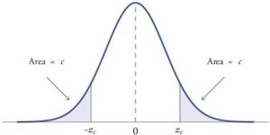
Figure 1. showing a 2-tail test for non-directional hypothesis for z for area C is the critical rejection region.
When a research hypothesis predicts a direction for the effect, it is called a directional hypothesis . To test the significance of a directional hypothesis, we have to consider the possibility that the sample could be extreme at one-tail of the comparison distribution. We call this a one-tailed test .
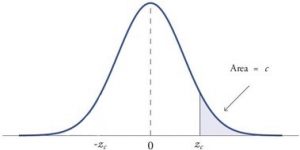
Figure 2. showing a 1-tail test for a directional hypothesis (predicting an increase) for z for area C is the critical rejection region.
Determining Cutoff Scores with Two-Tailed Tests
Typically we specify an α level before analyzing the data. If the data analysis results in a probability value below the α level, then the null hypothesis is rejected; if it is not, then the null hypothesis is not rejected. In other words, if our data produce values that meet or exceed this threshold, then we have sufficient evidence to reject the null hypothesis ; if not, we fail to reject the null (we never “accept” the null). According to this perspective, if a result is significant, then it does not matter how significant it is. Moreover, if it is not significant, then it does not matter how close to being significant it is. Therefore, if the 0.05 level is being used, then probability values of 0.049 and 0.001 are treated identically. Similarly, probability values of 0.06 and 0.34 are treated identically. Note we will discuss ways to address effect size (which is related to this challenge of NHST).
When setting the probability value, there is a special complication in a two-tailed test. We have to divide the significance percentage between the two tails. For example, with a 5% significance level, we reject the null hypothesis only if the sample is so extreme that it is in either the top 2.5% or the bottom 2.5% of the comparison distribution. This keeps the overall level of significance at a total of 5%. A one-tailed test does have such an extreme value but with a one-tailed test only one side of the distribution is considered.
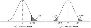
Figure 3. Critical value differences in one and two-tail tests. Photo Credit
Let’s re view th e set critical values for Z.
We discussed z-scores and probability in chapter 8. If we revisit the z-score for 5% and 1%, we can identify the critical regions for the critical rejection areas from the unit standard normal table.
- A two-tailed test at the 5% level has a critical boundary Z score of +1.96 and -1.96
- A one-tailed test at the 5% level has a critical boundary Z score of +1.64 or -1.64
- A two-tailed test at the 1% level has a critical boundary Z score of +2.58 and -2.58
- A one-tailed test at the 1% level has a critical boundary Z score of +2.33 or -2.33.
Review: Critical values, p-values, and significance level
There are two criteria we use to assess whether our data meet the thresholds established by our chosen significance level, and they both have to do with our discussions of probability and distributions. Recall that probability refers to the likelihood of an event, given some situation or set of conditions. In hypothesis testing, that situation is the assumption that the null hypothesis value is the correct value, or that there is no effec t. The value laid out in H 0 is our condition under which we interpret our results. To reject this assumption, and thereby reject the null hypothesis, we need results that would be very unlikely if the null was true.
Now recall that values of z which fall in the tails of the standard normal distribution represent unlikely values. That is, the proportion of the area under the curve as or more extreme than z is very small as we get into the tails of the distribution. Our significance level corresponds to the area under the tail that is exactly equal to α: if we use our normal criterion of α = .05, then 5% of the area under the curve becomes what we call the rejection region (also called the critical region) of the distribution. This is illustrated in Figure 4.

Figure 4: The rejection region for a one-tailed test
The shaded rejection region takes us 5% of the area under the curve. Any result which falls in that region is sufficient evidence to reject the null hypothesis.
The rejection region is bounded by a specific z-value, as is any area under the curve. In hypothesis testing, the value corresponding to a specific rejection region is called the critical value, z crit (“z-crit”) or z* (hence the other name “critical region”). Finding the critical value works exactly the same as finding the z-score corresponding to any area under the curve like we did in Unit 1. If we go to the normal table, we will find that the z-score corresponding to 5% of the area under the curve is equal to 1.645 (z = 1.64 corresponds to 0.0405 and z = 1.65 corresponds to 0.0495, so .05 is exactly in between them) if we go to the right and -1.645 if we go to the left. The direction must be determined by your alternative hypothesis, and drawing then shading the distribution is helpful for keeping directionality straight.
Suppose, however, that we want to do a non-directional test. We need to put the critical region in both tails, but we don’t want to increase the overall size of the rejection region (for reasons we will see later). To do this, we simply split it in half so that an equal proportion of the area under the curve falls in each tail’s rejection region. For α = .05, this means 2.5% of the area is in each tail, which, based on the z-table, corresponds to critical values of z* = ±1.96. This is shown in Figure 5.

Figure 5: Two-tailed rejection region
Thus, any z-score falling outside ±1.96 (greater than 1.96 in absolute value) falls in the rejection region. When we use z-scores in this way, the obtained value of z (sometimes called z-obtained) is something known as a test statistic, which is simply an inferential statistic used to test a null hypothesis.
Calculate the test statistic: Z
Now that we understand setting up the hypothesis and determining the outcome, let’s examine hypothesis testing with z! The next step is to carry out the study and get the actual results for our sample. Central to hypothesis test is comparison of the population and sample means. To make our calculation and determine where the sample is in the hypothesized distribution we calculate the Z for the sample data.
Make a decision
To decide whether to reject the null hypothesis, we compare our sample’s Z score to the Z score that marks our critical boundary. If our sample Z score falls inside the rejection region of the comparison distribution (is greater than the z-score critical boundary) we reject the null hypothesis.
The formula for our z- statistic has not changed:

To formally test our hypothesis, we compare our obtained z-statistic to our critical z-value. If z obt > z crit , that means it falls in the rejection region (to see why, draw a line for z = 2.5 on Figure 1 or Figure 2) and so we reject H 0 . If z obt < z crit , we fail to reject. Remember that as z gets larger, the corresponding area under the curve beyond z gets smaller. Thus, the proportion, or p-value, will be smaller than the area for α, and if the area is smaller, the probability gets smaller. Specifically, the probability of obtaining that result, or a more extreme result, under the condition that the null hypothesis is true gets smaller.
Conversely, if we fail to reject, we know that the proportion will be larger than α because the z-statistic will not be as far into the tail. This is illustrated for a one- tailed test in Figure 6.

Figure 6. Relation between α, z obt , and p
When the null hypothesis is rejected, the effect is said to be statistically significant . Do not confuse statistical significance with practical significance. A small effect can be highly significant if the sample size is large enough.
Why does the word “significant” in the phrase “statistically significant” mean something so different from other uses of the word? Interestingly, this is because the meaning of “significant” in everyday language has changed. It turns out that when the procedures for hypothesis testing were developed, something was “significant” if it signified something. Thus, finding that an effect is statistically significant signifies that the effect is real and not due to chance. Over the years, the meaning of “significant” changed, leading to the potential misinterpretation.
Review: Steps of the Hypothesis Testing Process
The process of testing hypotheses follows a simple four-step procedure. This process will be what we use for the remained of the textbook and course, and though the hypothesis and statistics we use will change, this process will not.
Step 1: State the Hypotheses
Your hypotheses are the first thing you need to lay out. Otherwise, there is nothing to test! You have to state the null hypothesis (which is what we test) and the alternative hypothesis (which is what we expect). These should be stated mathematically as they were presented above AND in words, explaining in normal English what each one means in terms of the research question.
Step 2: Find the Critical Values
Next, we formally lay out the criteria we will use to test our hypotheses. There are two pieces of information that inform our critical values: α, which determines how much of the area under the curve composes our rejection region, and the directionality of the test, which determines where the region will be.
Step 3: Compute the Test Statistic
Once we have our hypotheses and the standards we use to test them, we can collect data and calculate our test statistic, in this case z . This step is where the vast majority of differences in future chapters will arise: different tests used for different data are calculated in different ways, but the way we use and interpret them remains the same.
Step 4: Make the Decision
Finally, once we have our obtained test statistic, we can compare it to our critical value and decide whether we should reject or fail to reject the null hypothesis. When we do this, we must interpret the decision in relation to our research question, stating what we concluded, what we based our conclusion on, and the specific statistics we obtained.
Example: Movie Popcorn
Let’s see how hypothesis testing works in action by working through an example. Say that a movie theater owner likes to keep a very close eye on how much popcorn goes into each bag sold, so he knows that the average bag has 8 cups of popcorn and that this varies a little bit, about half a cup. That is, the known population mean is μ = 8.00 and the known population standard deviation is σ =0.50. The owner wants to make sure that the newest employee is filling bags correctly, so over the course of a week he randomly assesses 25 bags filled by the employee to test for a difference (n = 25). He doesn’t want bags overfilled or under filled, so he looks for differences in both directions. This scenario has all of the information we need to begin our hypothesis testing procedure.
Our manager is looking for a difference in the mean cups of popcorn bags compared to the population mean of 8. We will need both a null and an alternative hypothesis written both mathematically and in words. We’ll always start with the null hypothesis:
H 0 : There is no difference in the cups of popcorn bags from this employee H 0 : μ = 8.00
Notice that we phrase the hypothesis in terms of the population parameter μ, which in this case would be the true average cups of bags filled by the new employee.
Our assumption of no difference, the null hypothesis, is that this mean is exactly
the same as the known population mean value we want it to match, 8.00. Now let’s do the alternative:
H A : There is a difference in the cups of popcorn bags from this employee H A : μ ≠ 8.00
In this case, we don’t know if the bags will be too full or not full enough, so we do a two-tailed alternative hypothesis that there is a difference.
Our critical values are based on two things: the directionality of the test and the level of significance. We decided in step 1 that a two-tailed test is the appropriate directionality. We were given no information about the level of significance, so we assume that α = 0.05 is what we will use. As stated earlier in the chapter, the critical values for a two-tailed z-test at α = 0.05 are z* = ±1.96. This will be the criteria we use to test our hypothesis. We can now draw out our distribution so we can visualize the rejection region and make sure it makes sense

Figure 7: Rejection region for z* = ±1.96
Step 3: Calculate the Test Statistic
Now we come to our formal calculations. Let’s say that the manager collects data and finds that the average cups of this employee’s popcorn bags is ̅X = 7.75 cups. We can now plug this value, along with the values presented in the original problem, into our equation for z:
So our test statistic is z = -2.50, which we can draw onto our rejection region distribution:

Figure 8: Test statistic location
Looking at Figure 5, we can see that our obtained z-statistic falls in the rejection region. We can also directly compare it to our critical value: in terms of absolute value, -2.50 > -1.96, so we reject the null hypothesis. We can now write our conclusion:
When we write our conclusion, we write out the words to communicate what it actually means, but we also include the average sample size we calculated (the exact location doesn’t matter, just somewhere that flows naturally and makes sense) and the z-statistic and p-value. We don’t know the exact p-value, but we do know that because we rejected the null, it must be less than α.
Effect Size
When we reject the null hypothesis, we are stating that the difference we found was statistically significant, but we have mentioned several times that this tells us nothing about practical significance. To get an idea of the actual size of what we found, we can compute a new statistic called an effect size. Effect sizes give us an idea of how large, important, or meaningful a statistically significant effect is.
For mean differences like we calculated here, our effect size is Cohen’s d :
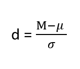
Effect sizes are incredibly useful and provide important information and clarification that overcomes some of the weakness of hypothesis testing. Whenever you find a significant result, you should always calculate an effect size
Table 1. Interpretation of Cohen’s d
Example: Office Temperature
Let’s do another example to solidify our understanding. Let’s say that the office building you work in is supposed to be kept at 74 degree Fahrenheit but is allowed
to vary by 1 degree in either direction. You suspect that, as a cost saving measure, the temperature was secretly set higher. You set up a formal way to test your hypothesis.
You start by laying out the null hypothesis:
H 0 : There is no difference in the average building temperature H 0 : μ = 74
Next you state the alternative hypothesis. You have reason to suspect a specific direction of change, so you make a one-tailed test:
H A : The average building temperature is higher than claimed H A : μ > 74

Now that you have everything set up, you spend one week collecting temperature data:
You calculate the average of these scores to be 𝑋̅ = 76.6 degrees. You use this to calculate the test statistic, using μ = 74 (the supposed average temperature), σ = 1.00 (how much the temperature should vary), and n = 5 (how many data points you collected):
z = 76.60 − 74.00 = 2.60 = 5.78
1.00/√5 0.45
This value falls so far into the tail that it cannot even be plotted on the distribution!

Figure 7: Obtained z-statistic
You compare your obtained z-statistic, z = 5.77, to the critical value, z* = 1.645, and find that z > z*. Therefore you reject the null hypothesis, concluding: Based on 5 observations, the average temperature (𝑋̅ = 76.6 degrees) is statistically significantly higher than it is supposed to be, z = 5.77, p < .05.
d = (76.60-74.00)/ 1= 2.60
The effect size you calculate is definitely large, meaning someone has some explaining to do!
Example: Different Significance Level
First, let’s take a look at an example phrased in generic terms, rather than in the context of a specific research question, to see the individual pieces one more time. This time, however, we will use a stricter significance level, α = 0.01, to test the hypothesis.
We will use 60 as an arbitrary null hypothesis value: H 0 : The average score does not differ from the population H 0 : μ = 50
We will assume a two-tailed test: H A : The average score does differ H A : μ ≠ 50
We have seen the critical values for z-tests at α = 0.05 levels of significance several times. To find the values for α = 0.01, we will go to the standard normal table and find the z-score cutting of 0.005 (0.01 divided by 2 for a two-tailed test) of the area in the tail, which is z crit * = ±2.575. Notice that this cutoff is much higher than it was for α = 0.05. This is because we need much less of the area in the tail, so we need to go very far out to find the cutoff. As a result, this will require a much larger effect or much larger sample size in order to reject the null hypothesis.
We can now calculate our test statistic. The average of 10 scores is M = 60.40 with a µ = 60. We will use σ = 10 as our known population standard deviation. From this information, we calculate our z-statistic as:
Our obtained z-statistic, z = 0.13, is very small. It is much less than our critical value of 2.575. Thus, this time, we fail to reject the null hypothesis. Our conclusion would look something like:
Notice two things about the end of the conclusion. First, we wrote that p is greater than instead of p is less than, like we did in the previous two examples. This is because we failed to reject the null hypothesis. We don’t know exactly what the p- value is, but we know it must be larger than the α level we used to test our hypothesis. Second, we used 0.01 instead of the usual 0.05, because this time we tested at a different level. The number you compare to the p-value should always be the significance level you test at. Because we did not detect a statistically significant effect, we do not need to calculate an effect size. Note: some statisticians will suggest to always calculate effects size as a possibility of Type II error. Although insignificant, calculating d = (60.4-60)/10 = .04 which suggests no effect (and not a possibility of Type II error).
Review Considerations in Hypothesis Testing
Errors in hypothesis testing.
Keep in mind that rejecting the null hypothesis is not an all-or-nothing decision. The Type I error rate is affected by the α level: the lower the α level the lower the Type I error rate. It might seem that α is the probability of a Type I error. However, this is not correct. Instead, α is the probability of a Type I error given that the null hypothesis is true. If the null hypothesis is false, then it is impossible to make a Type I error. The second type of error that can be made in significance testing is failing to reject a false null hypothesis. This kind of error is called a Type II error.
Statistical Power
The statistical power of a research design is the probability of rejecting the null hypothesis given the sample size and expected relationship strength. Statistical power is the complement of the probability of committing a Type II error. Clearly, researchers should be interested in the power of their research designs if they want to avoid making Type II errors. In particular, they should make sure their research design has adequate power before collecting data. A common guideline is that a power of .80 is adequate. This means that there is an 80% chance of rejecting the null hypothesis for the expected relationship strength.
Given that statistical power depends primarily on relationship strength and sample size, there are essentially two steps you can take to increase statistical power: increase the strength of the relationship or increase the sample size. Increasing the strength of the relationship can sometimes be accomplished by using a stronger manipulation or by more carefully controlling extraneous variables to reduce the amount of noise in the data (e.g., by using a within-subjects design rather than a between-subjects design). The usual strategy, however, is to increase the sample size. For any expected relationship strength, there will always be some sample large enough to achieve adequate power.
Inferential statistics uses data from a sample of individuals to reach conclusions about the whole population. The degree to which our inferences are valid depends upon how we selected the sample (sampling technique) and the characteristics (parameters) of population data. Statistical analyses assume that sample(s) and population(s) meet certain conditions called statistical assumptions.
It is easy to check assumptions when using statistical software and it is important as a researcher to check for violations; if violations of statistical assumptions are not appropriately addressed then results may be interpreted incorrectly.
Learning Objectives
Having read the chapter, students should be able to:
- Conduct a hypothesis test using a z-score statistics, locating critical region, and make a statistical decision including.
- Explain the purpose of measuring effect size and power, and be able to compute Cohen’s d.
Exercises – Ch. 10
- List the main steps for hypothesis testing with the z-statistic. When and why do you calculate an effect size?
- z = 1.99, two-tailed test at α = 0.05
- z = 1.99, two-tailed test at α = 0.01
- z = 1.99, one-tailed test at α = 0.05
- You are part of a trivia team and have tracked your team’s performance since you started playing, so you know that your scores are normally distributed with μ = 78 and σ = 12. Recently, a new person joined the team, and you think the scores have gotten better. Use hypothesis testing to see if the average score has improved based on the following 8 weeks’ worth of score data: 82, 74, 62, 68, 79, 94, 90, 81, 80.
- A study examines self-esteem and depression in teenagers. A sample of 25 teens with a low self-esteem are given the Beck Depression Inventory. The average score for the group is 20.9. For the general population, the average score is 18.3 with σ = 12. Use a two-tail test with α = 0.05 to examine whether teenagers with low self-esteem show significant differences in depression.
- You get hired as a server at a local restaurant, and the manager tells you that servers’ tips are $42 on average but vary about $12 (μ = 42, σ = 12). You decide to track your tips to see if you make a different amount, but because this is your first job as a server, you don’t know if you will make more or less in tips. After working 16 shifts, you find that your average nightly amount is $44.50 from tips. Test for a difference between this value and the population mean at the α = 0.05 level of significance.
Answers to Odd- Numbered Exercises – Ch. 10
1. List hypotheses. Determine critical region. Calculate z. Compare z to critical region. Draw Conclusion. We calculate an effect size when we find a statistically significant result to see if our result is practically meaningful or important
5. Step 1: H 0 : μ = 42 “My average tips does not differ from other servers”, H A : μ ≠ 42 “My average tips do differ from others”
Introduction to Statistics for Psychology Copyright © 2021 by Alisa Beyer is licensed under a Creative Commons Attribution-NonCommercial-ShareAlike 4.0 International License , except where otherwise noted.
Share This Book
Z test is a statistical test that is conducted on data that approximately follows a normal distribution. The z test can be performed on one sample, two samples, or on proportions for hypothesis testing. It checks if the means of two large samples are different or not when the population variance is known.
A z test can further be classified into left-tailed, right-tailed, and two-tailed hypothesis tests depending upon the parameters of the data. In this article, we will learn more about the z test, its formula, the z test statistic, and how to perform the test for different types of data using examples.
What is Z Test?
A z test is a test that is used to check if the means of two populations are different or not provided the data follows a normal distribution. For this purpose, the null hypothesis and the alternative hypothesis must be set up and the value of the z test statistic must be calculated. The decision criterion is based on the z critical value.
Z Test Definition
A z test is conducted on a population that follows a normal distribution with independent data points and has a sample size that is greater than or equal to 30. It is used to check whether the means of two populations are equal to each other when the population variance is known. The null hypothesis of a z test can be rejected if the z test statistic is statistically significant when compared with the critical value.
Z Test Formula
The z test formula compares the z statistic with the z critical value to test whether there is a difference in the means of two populations. In hypothesis testing , the z critical value divides the distribution graph into the acceptance and the rejection regions. If the test statistic falls in the rejection region then the null hypothesis can be rejected otherwise it cannot be rejected. The z test formula to set up the required hypothesis tests for a one sample and a two-sample z test are given below.
One-Sample Z Test
A one-sample z test is used to check if there is a difference between the sample mean and the population mean when the population standard deviation is known. The formula for the z test statistic is given as follows:
z = \(\frac{\overline{x}-\mu}{\frac{\sigma}{\sqrt{n}}}\). \(\overline{x}\) is the sample mean, \(\mu\) is the population mean, \(\sigma\) is the population standard deviation and n is the sample size.
The algorithm to set a one sample z test based on the z test statistic is given as follows:
Left Tailed Test:
Null Hypothesis: \(H_{0}\) : \(\mu = \mu_{0}\)
Alternate Hypothesis: \(H_{1}\) : \(\mu < \mu_{0}\)
Decision Criteria: If the z statistic < z critical value then reject the null hypothesis.
Right Tailed Test:
Alternate Hypothesis: \(H_{1}\) : \(\mu > \mu_{0}\)
Decision Criteria: If the z statistic > z critical value then reject the null hypothesis.
Two Tailed Test:
Alternate Hypothesis: \(H_{1}\) : \(\mu \neq \mu_{0}\)
Two Sample Z Test
A two sample z test is used to check if there is a difference between the means of two samples. The z test statistic formula is given as follows:
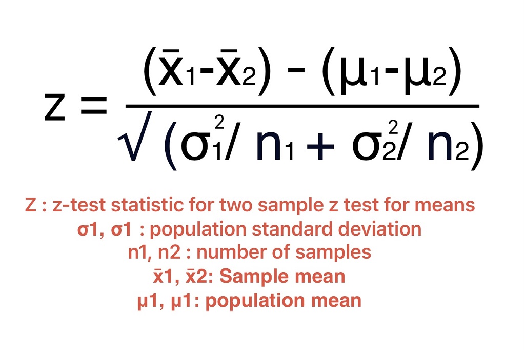
z = \(\frac{(\overline{x_{1}}-\overline{x_{2}})-(\mu_{1}-\mu_{2})}{\sqrt{\frac{\sigma_{1}^{2}}{n_{1}}+\frac{\sigma_{2}^{2}}{n_{2}}}}\). \(\overline{x_{1}}\), \(\mu_{1}\), \(\sigma_{1}^{2}\) are the sample mean, population mean and population variance respectively for the first sample. \(\overline{x_{2}}\), \(\mu_{2}\), \(\sigma_{2}^{2}\) are the sample mean, population mean and population variance respectively for the second sample.
The two-sample z test can be set up in the same way as the one-sample test. However, this test will be used to compare the means of the two samples. For example, the null hypothesis is given as \(H_{0}\) : \(\mu_{1} = \mu_{2}\).

Z Test for Proportions
A z test for proportions is used to check the difference in proportions. A z test can either be used for one proportion or two proportions. The formulas are given as follows.
One Proportion Z Test
A one proportion z test is used when there are two groups and compares the value of an observed proportion to a theoretical one. The z test statistic for a one proportion z test is given as follows:
z = \(\frac{p-p_{0}}{\sqrt{\frac{p_{0}(1-p_{0})}{n}}}\). Here, p is the observed value of the proportion, \(p_{0}\) is the theoretical proportion value and n is the sample size.
The null hypothesis is that the two proportions are the same while the alternative hypothesis is that they are not the same.
Two Proportion Z Test
A two proportion z test is conducted on two proportions to check if they are the same or not. The test statistic formula is given as follows:
z =\(\frac{p_{1}-p_{2}-0}{\sqrt{p(1-p)\left ( \frac{1}{n_{1}} +\frac{1}{n_{2}}\right )}}\)
where p = \(\frac{x_{1}+x_{2}}{n_{1}+n_{2}}\)
\(p_{1}\) is the proportion of sample 1 with sample size \(n_{1}\) and \(x_{1}\) number of trials.
\(p_{2}\) is the proportion of sample 2 with sample size \(n_{2}\) and \(x_{2}\) number of trials.
How to Calculate Z Test Statistic?
The most important step in calculating the z test statistic is to interpret the problem correctly. It is necessary to determine which tailed test needs to be conducted and what type of test does the z statistic belong to. Suppose a teacher claims that his section's students will score higher than his colleague's section. The mean score is 22.1 for 60 students belonging to his section with a standard deviation of 4.8. For his colleague's section, the mean score is 18.8 for 40 students and the standard deviation is 8.1. Test his claim at \(\alpha\) = 0.05. The steps to calculate the z test statistic are as follows:
- Identify the type of test. In this example, the means of two populations have to be compared in one direction thus, the test is a right-tailed two-sample z test.
- Set up the hypotheses. \(H_{0}\): \(\mu_{1} = \mu_{2}\), \(H_{1}\): \(\mu_{1} > \mu_{2}\).
- Find the critical value at the given alpha level using the z table. The critical value is 1.645.
- Determine the z test statistic using the appropriate formula. This is given by z = \(\frac{(\overline{x_{1}}-\overline{x_{2}})-(\mu_{1}-\mu_{2})}{\sqrt{\frac{\sigma_{1}^{2}}{n_{1}}+\frac{\sigma_{2}^{2}}{n_{2}}}}\). Substitute values in this equation. \(\overline{x_{1}}\) = 22.1, \(\sigma_{1}\) = 4.8, \(n_{1}\) = 60, \(\overline{x_{2}}\) = 18.8, \(\sigma_{2}\) = 8.1, \(n_{2}\) = 40 and \(\mu_{1} - \mu_{2} = 0\). Thus, z = 2.32
- Compare the critical value and test statistic to arrive at a conclusion. As 2.32 > 1.645 thus, the null hypothesis can be rejected. It can be concluded that there is enough evidence to support the teacher's claim that the scores of students are better in his class.
Z Test vs T-Test
Both z test and t-test are univariate tests used on the means of two datasets. The differences between both tests are outlined in the table given below:
Related Articles:
- Probability and Statistics
- Data Handling
- Summary Statistics
Important Notes on Z Test
- Z test is a statistical test that is conducted on normally distributed data to check if there is a difference in means of two data sets.
- The sample size should be greater than 30 and the population variance must be known to perform a z test.
- The one-sample z test checks if there is a difference in the sample and population mean,
- The two sample z test checks if the means of two different groups are equal.
Examples on Z Test
Example 1: A teacher claims that the mean score of students in his class is greater than 82 with a standard deviation of 20. If a sample of 81 students was selected with a mean score of 90 then check if there is enough evidence to support this claim at a 0.05 significance level.
Solution: As the sample size is 81 and population standard deviation is known, this is an example of a right-tailed one-sample z test.
\(H_{0}\) : \(\mu = 82\)
\(H_{1}\) : \(\mu > 82\)
From the z table the critical value at \(\alpha\) = 1.645
z = \(\frac{\overline{x}-\mu}{\frac{\sigma}{\sqrt{n}}}\)
\(\overline{x}\) = 90, \(\mu\) = 82, n = 81, \(\sigma\) = 20
As 3.6 > 1.645 thus, the null hypothesis is rejected and it is concluded that there is enough evidence to support the teacher's claim.
Answer: Reject the null hypothesis
Example 2: An online medicine shop claims that the mean delivery time for medicines is less than 120 minutes with a standard deviation of 30 minutes. Is there enough evidence to support this claim at a 0.05 significance level if 49 orders were examined with a mean of 100 minutes?
Solution: As the sample size is 49 and population standard deviation is known, this is an example of a left-tailed one-sample z test.
\(H_{0}\) : \(\mu = 120\)
\(H_{1}\) : \(\mu < 120\)
From the z table the critical value at \(\alpha\) = -1.645. A negative sign is used as this is a left tailed test.
\(\overline{x}\) = 100, \(\mu\) = 120, n = 49, \(\sigma\) = 30
As -4.66 < -1.645 thus, the null hypothesis is rejected and it is concluded that there is enough evidence to support the medicine shop's claim.
Example 3: A company wants to improve the quality of products by reducing defects and monitoring the efficiency of assembly lines. In assembly line A, there were 18 defects reported out of 200 samples while in line B, 25 defects out of 600 samples were noted. Is there a difference in the procedures at a 0.05 alpha level?
Solution: This is an example of a two-tailed two proportion z test.
\(H_{0}\): The two proportions are the same.
\(H_{1}\): The two proportions are not the same.
As this is a two-tailed test the alpha level needs to be divided by 2 to get 0.025.
Using this, the critical value from the z table is 1.96.
\(n_{1}\) = 200, \(n_{2}\) = 600
\(p_{1}\) = 18 / 200 = 0.09
\(p_{2}\) = 25 / 600 = 0.0416
p = (18 + 25) / (200 + 600) = 0.0537
z =\(\frac{p_{1}-p_{2}-0}{\sqrt{p(1-p)\left ( \frac{1}{n_{1}} +\frac{1}{n_{2}}\right )}}\) = 2.62
As 2.62 > 1.96 thus, the null hypothesis is rejected and it is concluded that there is a significant difference between the two lines.
go to slide go to slide go to slide

Book a Free Trial Class
FAQs on Z Test
What is a z test in statistics.
A z test in statistics is conducted on data that is normally distributed to test if the means of two datasets are equal. It can be performed when the sample size is greater than 30 and the population variance is known.
What is a One-Sample Z Test?
A one-sample z test is used when the population standard deviation is known, to compare the sample mean and the population mean. The z test statistic is given by the formula \(\frac{\overline{x}-\mu}{\frac{\sigma}{\sqrt{n}}}\).
What is the Two-Sample Z Test Formula?
The two sample z test is used when the means of two populations have to be compared. The z test formula is given as \(\frac{(\overline{x_{1}}-\overline{x_{2}})-(\mu_{1}-\mu_{2})}{\sqrt{\frac{\sigma_{1}^{2}}{n_{1}}+\frac{\sigma_{2}^{2}}{n_{2}}}}\).
What is a One Proportion Z test?
A one proportion z test is used to check if the value of the observed proportion is different from the value of the theoretical proportion. The z statistic is given by \(\frac{p-p_{0}}{\sqrt{\frac{p_{0}(1-p_{0})}{n}}}\).
What is a Two Proportion Z Test?
When the proportions of two samples have to be compared then the two proportion z test is used. The formula is given by \(\frac{p_{1}-p_{2}-0}{\sqrt{p(1-p)\left ( \frac{1}{n_{1}} +\frac{1}{n_{2}}\right )}}\).
How Do You Find the Z Test?
The steps to perform the z test are as follows:
- Set up the null and alternative hypotheses.
- Find the critical value using the alpha level and z table.
- Calculate the z statistic.
- Compare the critical value and the test statistic to decide whether to reject or not to reject the null hypothesis.
What is the Difference Between the Z Test and the T-Test?
A z test is used on large samples n ≥ 30 and normally distributed data while a t-test is used on small samples (n < 30) following a student t distribution . Both tests are used to check if the means of two datasets are the same.
- Privacy Policy
Z Test – Formula, Definition, Examples, Types
- 9 December 2023 28 December 2023
Table of Contents
What is Z Test
A z test is a statistical test in hypothesis testing to determine whether two population means are different when the population variance is known and the sample size is large.
Z-tests are similar to t-tests. T-tests are used when we have a small sample size and the standard deviation is unknown.
When to use the z test
We can use z test for hypothesis testing if the following prior conditions are met.
- Normal distribution of data
- All data points are independent
- Standard deviation is known
- Sample Size ≥ 30
- Equal sample variance
As per the central limit theorem, as we increase the number of samples, there is more probability the data is normally distributed. Therefore we need more than 30 samples in the z-test for hypothesis testing to ensure the data is normally distributed.
If the population variance is unknown, we can still use the Z Test by estimating the population variance from the sample data. This is possible only if the number of sample data points is greater than 30.
Relation between z-score and Margin of Error
We can use the z-score to calculate the margin of error .
The margin of error = 2 x Standard deviation for sample distribution
Standard deviation for sample distribution = Population Standard Deviation / √n
Steps to conduct the Z-test
Here is the list of steps we use to conduct the z-test in hypothesis testing.
- Get the data
- Check for prior conditions
- Define null and alternative hypotheses
- Finalize a significant level or alpha
- Get the z-score
- Calculate the z-test statistic
- Evaluate the results
What Is a Z-Score?
The z-score or z-statistic is a number that represents how many standard deviations above or below a data point is from the population mean in normal distribution.
Significance of Z-test in Machine Learning
We can use hypothesis testing or z-test in machine learning to:
- Evaluate the ML model’s performance
- Determine ML model parameters’ significance.
- Evaluate a model’s accuracy
- Test the statistical validity of machine learning algorithms like linear regression and logistic regression.
We can use a z-test to compare the means of two data groups to determine if there is a significant difference between them. We can Improve the ML model using this information, or select the best set of features.
Types of Z Test in Hypothesis Testing
Here is the list of various types of z-test for hypothesis testing.
- Z-test for Means
- Z-test for Proportions

Z Test for Means
We use z-test for means to compare the means of two samples or sample and the population mean. We can further classify z test for means into two types:
- One sample z test for means
- Two Sample z test for means
One-Sample Z-Test for Means
One-sample z-test is used to compare the sample mean with the population mean. In other words, it checks whether the sample belongs to the given population using Z-statistics. This test is similar to one-sample t-test .

In this test, we try to determine how far the sample mean is from the population mean in terms of the number of standard deviations. Afterward, we determine if this deviation is statistically significant by comparing z-statistics and critical values.
Calculation Formula

We can use one sample z-test to determine:
- If the average part diameter is 15mm.
- Whether the average monthly stock return is greater than 2%.
Problem Statement Example
Determine if a packing average weight is 50 grams considering we have sample weight data for 35 samples. From production data, we know that the standard deviation for packing weight is 1.5.
Here we can use z test to prove or reject the statement.
Step-1: Get the Sample Data
We collect 35 packings randomly from the production line and record their weight.
50, 49, 51, 49.5, 49, 48.8, 51.2, 50.8, 50.6, 49.95, 50.1, 50.9, 47.3, 47.6, 50, 51.2, 50.8, 50.6, 49, 48.8, 51.2, 50.8, 50.5, 49.95, 50.12, 50.9, 47.8, 47.6, 50, 49.2, 47.8, 48, 48.5, 51.2, 50.2
Step-2: Check if we can use the z test
Next step to to check if we can use the z-test for this hypothesis testing.
- Normal distribution of data : Test of normality is found ok
- All data points are independent : Yes independent samples are considered.
- Standard deviation is known : Yes, value is given in problem statement
- Sample Size ≥ 30 : yes
- Equal sample variance : Not applicable for one sample test
Step-3: Define null and Alternative Hypotheses
Null Hypothesis: Packing Average weight is not equal to 50 grams.
Alternate Hypothesis: Packing Average weight is equal to 50 grams.
Step-4: Finalize Alpha
We are considering alpha = 0.05
Step-5: Calculate the z-statistic
Sample Mean = 49.72971, Population Mean = 50, Population Standard Deviation = 1.5, n = 35
Z-Statistics = (49.729 – 50) / (1.5 / √351) = – 0.271 / 0.2535 = -1.059
Step-6: Calculate the critical z-score or p-value from the Z-table
p-value for z-statistic(-1.059) = .2896
We suggest you read this article on how to calculate critical value and p-value from the z-table.
Step-7: Evaluate the results
Calculated p-value (.2896) > alpha (0.05)
The test results are not statistically significant and we can not reject the null hypothesis.
Two-Sample Z Test for means
A two-sample z-test is used to compare the means of two samples. We can use two sample z-tests for means to determine whether the means of two populations that generated the two samples are equal or different. This test is similar to an independent two-sample t-test .

Application Examples
Here is the list of application examples of two sample z-tests for means.
- Determine if there is a difference in average wait time at two restaurants.
- If there is a difference of 5 grams in packing average weight from two different machines (machine-1 and machine-2). From production data, we know that the average package weight from two machines is 45 grams and 50 grams respectively whereas a standard deviation of 1.5 and 1.3 is observed.
- If the average salary of the two groups is based on gender (male and female).
- Compare a website’s earnings with two different layouts.
- Compare the performance of two sections in a class.
Null and Alternate Hypothesis for two Sample z-test
Null hypothesis: There is no significant difference in the means of the two populations. => μ1 – μ2= 0
Alternate hypothesis: The means of the two populations are significantly different => μ1 – μ2≠ 0
Two sample z test for means calculation formula
Z Test for Proportions
We use z-test for proportions to compare proportions for two samples or sample and the hypothesized proportions. We can further classify z test for means into two types:
- One sample z test for proportions
- Two Sample z test for proportions
One-Sample Z-Test for Proportions
One-sample Z-test for proportion is a hypothesis test used to compare hypothesized proportion to a given theoretical population proportion. In other words, it checks whether there is a difference in hypothesized or sample proportion and population proportion.
We can use z-test to answer the following questions:
- Is there any difference in sample proportion and population proportion?
- Is the difference between population and sample proportion statistically significant?
Calculation formula for One sample z-test for proportions

Application Example for One sample z-test for proportion
A quality engineer wants to check whether there is a difference between population and sample proportion for the rejection rate for parts manufactured on a production line. The rejected part proportion is 5% during production, whereas it was 8% when we selected 50 random samples.
Is this difference in proportion statistically significant if the Level of Significance is 0.05?
Step-1: Collect the required data
Population Proportion (Po) = 0.05, Sample Proportion (P) = 0.08, number of samples (n) = 50, alpha = 0.05
The next step to to check for the following prior conditions to conduct the z-test.
- Standard deviation is known : Yes, the value is given in the problem statement
- Equal sample variance : Yes
Step-3: Define null and alternative hypotheses
Null Hypothesis: There is no difference between the sample and production parts.
Alternate Hypothesis: Sample and production parts are different.
Step-4: Finalize alpha
Considering our application, we are considering alpha=0.05
Z-Statistics = (P – Po) / √ [Po (1 – Po) / n] = (0.08 – 0.05) / √ [0.05 * (1-0.05) / 50]
Z-Statistics = 0.03 / √ (0.000095) = 0.03 / 0.0308 = 0.974
Step-6: Calculate the critical value
p-value for z-statistic(0.974) = .330
Calculated p-value (.330) > alpha (0.05)
We can use z-test for proportions to determine whether the proportion of government school students passing the IIT exam is similar to national proportion.
Two-Sample Z-Test for Proportions
Two-sample z-test for proportions is a hypothesis test that is used to determine if two samples are from the same population. We need population proportions for this test. We do not require any information on population standard deviation.
We can use this test for the following applications:
- Compare the proportion of users in two groups who can buy a product when they visit the store.
- A/B Testing: Compare reviews about a product on two user groups.
Null and Alternate Hypothesis for two Sample Z-test
Null hypothesis: Two populations are equal. => μ1 – μ2=0
Alternate hypothesis: The means of two populations are significantly different => μ1 – μ2=0

Application Example for Two-Sample Z-Test for Proportions
A marketing person wants to determine how different age groups customers think about a new product. We can use the two-proportion z test to determine if the proportion of customers who think positively about a new product is different in two groups.
In the first sample of 150 customers, 100 customers think positively about the product. Whereas, for the second sample of 200 customers 110 customers think positively about a new product.
Z-test Statistic Calculation
p̂1 = 100 / 150 = 0.66, p̂2 = 110 / 200 = 0.55, p̂ = (100+110) / (150+200) = 0.6
Z-Statistics = (p̂1 – p̂2) / √ [p (1-p) (1/n1 + 1/n2]]
Z-Statistics = (0.66 — 0.55) / √ [0.6 (1-0.6) (1/150 + 1/200)]
= 0.11 / √ [0.6 * 0.4 (0.0066+0.005)] = 0.11 / √ [0.6*0.4*0.0116]
= 0.11 / √ [0.6 * 0.4 * 0.0116] = 0.11 / 0.0431 = 2.55
P-value calculation from z-table
p-value for z-statistic(2.55) = .010772
Results Evaluation
Calculated p-value (.010772) < alpha (0.05)
The test results are statistically significant and we can reject the null hypothesis. In other words two populations are statistically different
Key Takeaways
We use the z-test in hypothesis testing to evaluate whether the test results are statistically significant or not. In other words, it checks whether the mean of two groups or a group and value is similar.
- Z-test is a statistical test to determine whether two population means are different when the variances are known and the sample size is large.
- Z-statistic follows a normal distribution.
- In Z-tests assume that the population standard deviation is known.
Frequently Asked Questions on Z-Test
We can find the critical z-score from the z-table in the following steps.
Step-1: Get a confidence level
Step-2: Calculate the area under the z-distribution curve to the left.
Step-3: Look for the calculated area in the z-table.
Step-4: The sum of the corresponding values for the calculated area is the value of critical z-score.
We suggest you read this article on how to read the z-table for more details .
Yes, you can use the z-test when the number of samples is less than 30 if the population variance is known. The z-test is typically used when working with a normal distribution and known population parameters.
Z-test is preferred over t-test in following conditions:
- Large sample size.
- Population variance is known.
- Normal distribution of data.
The z-distribution is normal distribution with “0” mean and “1” standard deviation. The t-distribution shape is similar to the normal distribution with heavier tails. T-distribution shape depends on the data degrees of freedom.
We can use one sample z-test for means to determine:
Two sample z-tests for means can be used in the following conditions.
- Compare a website’s earnings with two different layouts or the performance of two sections in a class.
We can use one sample z-test for proportion to:
- Determine if the sample rejection proportion is similar to the part rejection proportion during production.
- Whether the proportion of government school students passing the IIT exam is similar to the national proportion.
We can use two sample z-test for proportion to:
- Compare the review of a product from two age group of peoples.
We can use two sample z-test for means to compare the accuracy of two machine learning algorithms on a given data.
Leave a Reply Cancel reply
Your email address will not be published. Required fields are marked *
Save my name, email, and website in this browser for the next time I comment.
Introduction to Statistics and Data Analysis
6 hypothesis testing: the z-test.
We’ve all had the experience of standing at a crosswalk waiting staring at a pedestrian traffic light showing the little red man. You’re waiting for the little green man so you can cross. After a little while you’re still waiting and there aren’t any cars around. You might think ‘this light is really taking a long time’, but you continue waiting. Minutes pass and there’s still no little green man. At some point you come to the conclusion that the light is broken and you’ll never see that little green man. You cross on the little red man when it’s clear.
You may not have known this but you just conducted a hypothesis test. When you arrived at the crosswalk, you assumed that the light was functioning properly, although you will always entertain the possibility that it’s broken. In terms of hypothesis testing, your ‘null hypothesis’ is that the light is working and your ‘alternative hypothesis’ is that it’s broken. As time passes, it seems less and less likely that light is working properly. Eventually, the probability of the light working given how long you’ve been waiting becomes so low that you reject the null hypothesis in favor of the alternative hypothesis.
This sort of reasoning is the backbone of hypothesis testing and inferential statistics. It’s also the point in the course where we turn the corner from descriptive statistics to inferential statistics. Rather than describing our data in terms of means and plots, we will now start using our data to make inferences, or generalizations, about the population that our samples are drawn from. In this course we’ll focus on standard hypothesis testing where we set up a null hypothesis and determine the probability of our observed data under the assumption that the null hypothesis is true (the much maligned p-value). If this probability is small enough, then we conclude that our data suggests that the null hypothesis is false, so we reject it.
In this chapter, we’ll introduce hypothesis testing with examples from a ‘z-test’, when we’re comparing a single mean to what we’d expect from a population with known mean and standard deviation. In this case, we can convert our observed mean into a z-score for the standard normal distribution. Hence the name z-test.
It’s time to introduce the hypothesis test flow chart . It’s pretty self explanatory, even if you’re not familiar with all of these hypothesis tests. The z-test is (1) based on means, (2) with only one mean, and (3) where we know \(\sigma\) , the standard deviation of the population. Here’s how to find the z-test in the flow chart:

6.1 Women’s height example
Let’s work with the example from the end of the last chapter where we started with the fact that the heights of US women has a mean of 63 and a standard deviation of 2.5 inches. We calculated that the average height of the 122 women in Psych 315 is 64.7 inches. We then used the central limit theorem and calculated the probability of a random sample 122 heights from this population having a mean of 64.7 or greater is 2.4868996^{-14}. This is a very, very small number.
Here’s how we do it using R:
Let’s think of our sample as a random sample of UW psychology students, which is a reasonable assumption since all psychology students have to take a statistics class. What does this sample say about the psychology students that are women at UW compared to the US population? It could be that these psychology students at UW have the same mean and standard deviation as the US population, but our sample just happens to have an unusual number of tall women, but we calculated that the probability of this happening is really low. Instead, it makes more sense that the population that we’re drawing from has a mean that’s greater than the US population mean. Notice that we’re making a conclusion about the whole population of women psychology students based on our one sample.
Using the terminology of hypothesis testing, we first assumed the null hypothesis that UW women psych students have the same mean (and standard deviation) as the US population. The null hypothesis is written as:
\[ H_{0}: \mu = 63 \] In this example, our alternative hypothesis is that the mean of our population is larger than the mean of null hypothesis population. We write this as:
\[ H_{A}: \mu > 63 \]
Next, after obtaining a random sample and calculate the mean, we calculate the probability of drawing a mean this large (or larger) from the null hypothesis distribution.
If this probability is low enough, we reject the null hypothesis in favor of the alternative hypothesis. When our probability allows us to reject the null hypothesis, we say that our observed results are ‘statistically significant’.
In statistics terms, we never say we ‘accept that alternative hypothesis’ as true. All we can say is that we don’t think the null hypothesis is true. I know it’s subtle, but in science can never prove that a hypothesis is true or not. There’s always the possibility that we just happened to grab an unusual sample from the null hypothesis distribution.
6.2 The hated p<.05
The probability that we obtain our observed mean or greater given that the null hypothesis is true is called the p-value. How improbable is improbable enough to reject the null hypothesis? The p-value for our example above on women’s heights is astronomically low, so it’s clear that we should reject \(H_{0}\) .
The p-value that’s on the border of rejection is called the alpha ( \(\alpha\) ) value. We reject \(H_{0}\) when our p-value is less than \(\alpha\) .
You probably know that the most common value of alpha is \(\alpha = .05\) .
The first publication of this value dates back to Sir Ronald Fisher, in his seminal 1925 book Statistical Methods for Research Workers where he states:
“It is convenient to take this point as a limit in judging whether a deviation is considered significant or not. Deviations exceeding twice the standard deviation are thus formally regarded as significant.” (p. 47)
If you read the chapter on the normal distribution, then you should know that 95% of the area under the normal distribution lies within \(\pm\) two standard deviations of the mean. So the probability of obtaining a sample that exceeds two standard deviations from the mean (in either direction) is .05.
6.3 IQ example
Let’s do an example using IQ scores. IQ scores are normalized to have a mean of 100 and a standard deviation of 15 points. Because they’re normalized, they are a rare example of a population which has a known mean and standard deviation. In the next chapter we’ll discuss the t-test, which is used in the more common situation when we don’t know the population standard deviation.
Suppose you have the suspicion that graduate students have higher IQ’s than the general population. You have enough time to go and measure the IQ’s of 25 randomly sampled grad students and obtain a mean of 105. Is this difference between our this observed mean and 100 statistically significant using an alpha value of \(\alpha = 0.05\) ?
Here the null hypothesis is:
\[ H_{0}: \mu = 100\]
And the alternative hypothesis is:
\[ H_{A}: \mu > 100 \]
We know that the parameters for the null hypothesis are:
\[ \mu = 100 \] and \[ \sigma = 15 \]
From this, we can calculate the probability of observing our mean of 105 or higher using the central limit theorem and what we know about the normal distribution:
\[ \sigma_{\bar{x}} = \frac{\sigma_{x}}{\sqrt{n}} = \frac{15}{\sqrt{25}} = 3 \] From this, we can calculate the probability of our observed mean using R’s ‘pnorm’ function. Here’s how to do the whole thing in R.
Since our p-value of 0.0478 is (just barely) less than our chosen value of \(\alpha = 0.05\) as our criterion, we reject \(H_{0}\) for this (contrived) example and conclude that our observed mean of 105 is significantly greater than 100, so our study suggests that the average graduate student has a higher IQ than the overall population.
You should feel uncomfortable making such a hard, binary decision for such a borderline case. After all, if we had chosen our second favorite value of alpha, \(\alpha = .01\) , we would have failed to reject \(H_{0}\) . This discomfort is a primary reason why statisticians are moving away from this discrete decision making process. Later on we’ll discuss where things are going, including reporting effect sizes, and using confidence intervals.
6.4 Alpha values vs. critical values
Using R’s qnorm function, we can find the z-score for which only 5% of the area lies above:
So the probability of a randomly sampled z-score exceeding 1.644854 is less than 5%. It follows that if we convert our observed mean into z-score values, we will reject \(H_{0}\) if and only if our z-score is greater than 1.644854. This value is called the ‘critical value’ because it lies on the boundary between rejecting and failing to reject \(H_{0}\) .
In our last example, the z-score for our observed mean is:
\[ z = \frac{X-\mu}{\frac{\sigma}{\sqrt{n}}} = \frac{105 - 100}{3} = 1.67 \] Our z-score is just barely greater than the critical value of 1.644854, which makes sense because our p-value is just barely less than 0.05.
Sometimes you’ll see textbooks will compare critical values to observed scores for the decision making process in hypothesis testing. This dates back to days were computers were less available and we had to rely on tables instead. There wasn’t enough space in a book to hold complete tables which prohibited the ability to look up a p-value for any observed value. Instead only critical values for specific values of alpha were included. If you look at really old papers, you’ll see statistics reported as \(p<.05\) or \(p<.01\) instead of actual p-values for this reason.
It may help to visualize the relationship between p-values, alpha values and critical values like this:

The red shaded region is the upper 5% of the standard normal distribution which starts at the critical value of z=1.644854. This is sometimes called the ‘rejection region’. The blue vertical line is drawn at our observed value of z=1.67. You can see that the red line falls just inside the rejection region, so we Reject \(H_{0}\) !
6.5 One vs. two-tailed tests
Recall that our alternative hypothesis was to reject if our mean IQ was significantly greater than the null hypothesis mean: \(H_{A}: \mu > 100\) . This implies that the situation where \(\mu < 100\) is never even in consideration, which is weird. In science, we’re trying to understand the true state of the world. Although we have a hunch that grad student IQ’s are higher than average, there is always the possibility that they are lower than average. If our sample came up with an IQ well below 100, we’d simply fail to reject \(H_{0}\) and move on. This feels like throwing out important information.
The test we just ran is called a ‘one-tailed’ test because we only reject \(H_{0}\) if our results fall in one of the two tails of the population distribution.
Instead, it might make more sense to reject \(H_{0}\) if we get either an unusually large or small score. This means we need two critical values - one above and one below zero. At first thought you might think we just duplicate our critical value from a one-tailed test to the other side. But will double the area of the rejection region. That’s not a good thing because if \(H_{0}\) is true, there’s actually a \(2\alpha\) probability that we’ll draw a score in the rejection region.
Instead, we divide the area into two tails, each containing an area of \(\frac{\alpha}{2}\) . For \(\alpha\) = 0.05, we can find the critical value of z with qnorm:
So with a two-tailed test at \(\alpha = 0.05\) we reject \(H_{0}\) if our observed z-score is either above z = 1.96 or less than -1.96. This is that value around 2 that Sir Ronald Fischer was talking about!
Here’s what the critical regions and observed value of z looks like for our example with a two-tailed test:

You can see that splitting the area of \(\alpha = 0.05\) into two halves increased the critical value in the positive direction from 1.64 to 1.96, making it harder to reject \(H_{0}\) . For our example, this changes our decision: our observed value of z = 1.67 no longer falls into the rejection region, so now we fail to reject \(H_{0}\) .
If we now fail to reject \(H_{0}\) , what about the p-value? Remember, for a one-tailed test, p = \(\alpha\) if our observed z-score lands right on the critical value of z. The same is true for a two-tailed test. But the z-score moved so that the area above that score is \(\frac{\alpha}{2}\) . So for a two-tailed test, in order to have a p-value of \(\alpha\) when our z-score lands right on the critical value, we need to double p-value hat we’d get for a one-tailed test.
For our example, the p-value for the one tailed test was \(p=0.0478\) . So if we use a two-tailed test, our p-value is \((2)(0.0478) = 0.0956\) . This value is greater than \(\alpha\) = 0.05, which makes sense because we just showed above that we fail to reject \(H_{0}\) with a two tailed test.
Which is the right test, one-tailed or two-tailed? Ideally, as scientists, we should be agnostic about the results of our experiment. But in reality, we all know that the results are more interesting if they are statistically significant. So you can imagine that for this example, given a choice between one and two-tailed, we’d choose a one-tailed test so that we can reject \(H_{0}\) .
There are two problems with this. First, we should never adjust our choice of hypothesis test after we observe the data. That would be an example of ‘p-hacking’, a topic we’ll discuss later. Second, most statisticians these days strongly recommend against one-tailed tests. The only reason for a one-tailed test is if there is no logical or physical possibility for a population mean to fall below the null hypothesis mean.
User Preferences
Content preview.
Arcu felis bibendum ut tristique et egestas quis:
- Ut enim ad minim veniam, quis nostrud exercitation ullamco laboris
- Duis aute irure dolor in reprehenderit in voluptate
- Excepteur sint occaecat cupidatat non proident
Keyboard Shortcuts
1.2 - the 7 step process of statistical hypothesis testing.
We will cover the seven steps one by one.
Step 1: State the Null Hypothesis
The null hypothesis can be thought of as the opposite of the "guess" the researchers made. In the example presented in the previous section, the biologist "guesses" plant height will be different for the various fertilizers. So the null hypothesis would be that there will be no difference among the groups of plants. Specifically, in more statistical language the null for an ANOVA is that the means are the same. We state the null hypothesis as:
\(H_0 \colon \mu_1 = \mu_2 = ⋯ = \mu_T\)
for T levels of an experimental treatment.
Step 2: State the Alternative Hypothesis
\(H_A \colon \text{ treatment level means not all equal}\)
The alternative hypothesis is stated in this way so that if the null is rejected, there are many alternative possibilities.
For example, \(\mu_1\ne \mu_2 = ⋯ = \mu_T\) is one possibility, as is \(\mu_1=\mu_2\ne\mu_3= ⋯ =\mu_T\). Many people make the mistake of stating the alternative hypothesis as \(\mu_1\ne\mu_2\ne⋯\ne\mu_T\) which says that every mean differs from every other mean. This is a possibility, but only one of many possibilities. A simple way of thinking about this is that at least one mean is different from all others. To cover all alternative outcomes, we resort to a verbal statement of "not all equal" and then follow up with mean comparisons to find out where differences among means exist. In our example, a possible outcome would be that fertilizer 1 results in plants that are exceptionally tall, but fertilizers 2, 3, and the control group may not differ from one another.
Step 3: Set \(\alpha\)
If we look at what can happen in a hypothesis test, we can construct the following contingency table:
You should be familiar with Type I and Type II errors from your introductory courses. It is important to note that we want to set \(\alpha\) before the experiment ( a-priori ) because the Type I error is the more grievous error to make. The typical value of \(\alpha\) is 0.05, establishing a 95% confidence level. For this course, we will assume \(\alpha\) =0.05, unless stated otherwise.
Step 4: Collect Data
Remember the importance of recognizing whether data is collected through an experimental design or observational study.
Step 5: Calculate a test statistic
For categorical treatment level means, we use an F- statistic, named after R.A. Fisher. We will explore the mechanics of computing the F- statistic beginning in Lesson 2. The F- value we get from the data is labeled \(F_{\text{calculated}}\).
Step 6: Construct Acceptance / Rejection regions
As with all other test statistics, a threshold (critical) value of F is established. This F- value can be obtained from statistical tables or software and is referred to as \(F_{\text{critical}}\) or \(F_\alpha\). As a reminder, this critical value is the minimum value of the test statistic (in this case \(F_{\text{calculated}}\)) for us to reject the null.
The F- distribution, \(F_\alpha\), and the location of acceptance/rejection regions are shown in the graph below:
Step 7: Based on Steps 5 and 6, draw a conclusion about \(H_0\)
If \(F_{\text{calculated}}\) is larger than \(F_\alpha\), then you are in the rejection region and you can reject the null hypothesis with \(\left(1-\alpha \right)\) level of confidence.
Note that modern statistical software condenses Steps 6 and 7 by providing a p -value. The p -value here is the probability of getting an \(F_{\text{calculated}}\) even greater than what you observe assuming the null hypothesis is true. If by chance, the \(F_{\text{calculated}} = F_\alpha\), then the p -value would be exactly equal to \(\alpha\). With larger \(F_{\text{calculated}}\) values, we move further into the rejection region and the p- value becomes less than \(\alpha\). So, the decision rule is as follows:
If the p- value obtained from the ANOVA is less than \(\alpha\), then reject \(H_0\) in favor of \(H_A\).
- Practice Mathematical Algorithm
- Mathematical Algorithms
- Pythagorean Triplet
- Fibonacci Number
- Euclidean Algorithm
- LCM of Array
- GCD of Array
- Binomial Coefficient
- Catalan Numbers
- Sieve of Eratosthenes
- Euler Totient Function
- Modular Exponentiation
- Modular Multiplicative Inverse
- Stein's Algorithm
- Juggler Sequence
- Chinese Remainder Theorem
- Quiz on Fibonacci Numbers
- Machine Learning Mathematics
Linear Algebra and Matrix
- Scalar and Vector
- Python Program to Add Two Matrices
- Python program to multiply two matrices
- Vector Operations
- Product of Vectors
- Scalar Product of Vectors
- Dot and Cross Products on Vectors
- Transpose a matrix in Single line in Python
- Transpose of a Matrix
- Adjoint and Inverse of a Matrix
- How to inverse a matrix using NumPy
- Determinant of a Matrix
- Program to find Normal and Trace of a matrix
- Data Science | Solving Linear Equations
- Data Science - Solving Linear Equations with Python
- System of Linear Equations
- System of Linear Equations in three variables using Cramer's Rule
- Eigenvalues
- Applications of Eigenvalues and Eigenvectors
- How to compute the eigenvalues and right eigenvectors of a given square array using NumPY?
Statistics for Machine Learning
- Descriptive Statistic
- Measures of Central Tendency
- Measures of Dispersion | Types, Formula and Examples
- Mean, Variance and Standard Deviation
- Calculate the average, variance and standard deviation in Python using NumPy
- Random Variables
- Difference between Parametric and Non-Parametric Methods
- Probability Distribution
- Confidence Interval
- Mathematics | Covariance and Correlation
- Program to find correlation coefficient
- Robust Correlation
- Normal Probability Plot
- Quantile Quantile plots
- True Error vs Sample Error
- Bias-Variance Trade Off - Machine Learning
- Understanding Hypothesis Testing
- Paired T-Test - A Detailed Overview
- P-value in Machine Learning
- F-Test in Statistics
- Residual Leverage Plot (Regression Diagnostic)
- Difference between Null and Alternate Hypothesis
- Mann and Whitney U test
- Wilcoxon Signed Rank Test
- Kruskal Wallis Test
- Friedman Test
- Mathematics | Probability
Probability and Probability Distributions
- Mathematics - Law of Total Probability
- Bayes's Theorem for Conditional Probability
- Mathematics | Probability Distributions Set 1 (Uniform Distribution)
- Mathematics | Probability Distributions Set 4 (Binomial Distribution)
- Mathematics | Probability Distributions Set 5 (Poisson Distribution)
- Uniform Distribution Formula
- Mathematics | Probability Distributions Set 2 (Exponential Distribution)
- Mathematics | Probability Distributions Set 3 (Normal Distribution)
- Mathematics | Beta Distribution Model
- Gamma Distribution Model in Mathematics
- Chi-Square Test for Feature Selection - Mathematical Explanation
- Student's t-distribution in Statistics
- Python - Central Limit Theorem
- Mathematics | Limits, Continuity and Differentiability
- Implicit Differentiation
Calculus for Machine Learning
- Engineering Mathematics - Partial Derivatives
- Advanced Differentiation
- How to find Gradient of a Function using Python?
- Optimization techniques for Gradient Descent
- Higher Order Derivatives
- Taylor Series
- Application of Derivative - Maxima and Minima | Mathematics
- Absolute Minima and Maxima
- Optimization for Data Science
- Unconstrained Multivariate Optimization
- Lagrange Multipliers
- Lagrange's Interpolation
- Linear Regression in Machine learning
- Ordinary Least Squares (OLS) using statsmodels
Regression in Machine Learning
Different tests are used in statistics to compare distinct samples or groups and make conclusions about populations. These tests, also referred to as statistical tests, concentrate on examining the probability or possibility of acquiring the observed data under particular premises or hypotheses. They offer a framework for evaluating the evidence for or against a given hypothesis.
A statistical test starts with the formulation of a null hypothesis (H0) and an alternative hypothesis (Ha). The alternative hypothesis proposes a particular link or effect, whereas the null hypothesis reflects the default assumption and often states no effect or no difference.
The p-value indicates the likelihood of observing the data or more extreme results assuming the null hypothesis is true. Researchers compare the calculated p-value to a predetermined significance level, often denoted as α, to make a decision regarding the null hypothesis. If the p-value is smaller than α, the results are considered statistically significant, leading to the rejection of the null hypothesis in favor of the alternative hypothesis.
The p-value is calculated using a variety of statistical tests, including the Z-test, T-test , Chi-squared test , ANOVA , Z-test , and F-test , among others. In this article, we will focus on explaining the Z-test.
What is Z-Test?
Z-test is a statistical test that is used to determine whether the mean of a sample is significantly different from a known population mean when the population standard deviation is known. It is particularly useful when the sample size is large (>30).
Z-test can also be defined as a statistical method that is used to determine whether the distribution of the test statistics can be approximated using the normal distribution or not. It is the method to determine whether two sample means are approximately the same or different when their variance is known and the sample size is large (should be >= 30).
The Z-test compares the difference between the sample mean and the population means by considering the standard deviation of the sampling distribution. The resulting Z-score represents the number of standard deviations that the sample mean deviates from the population mean. This Z-Score is also known as Z-Statistics, and can be formulated as:

The average family annual income in India is 200k, with a standard deviation of 5k, and the average family annual income in Delhi is 300k.
Then Z-Score for Delhi will be.

This indicates that the average family’s annual income in Delhi is 20 standard deviations above the mean of the population (India).
When to Use Z-test:
- The sample size should be greater than 30. Otherwise, we should use the t-test.
- Samples should be drawn at random from the population.
- The standard deviation of the population should be known.
- Samples that are drawn from the population should be independent of each other.
- The data should be normally distributed , however, for a large sample size, it is assumed to have a normal distribution because central limit theorem
Hypothesis Testing
A hypothesis is an educated guess/claim about a particular property of an object. Hypothesis testing is a way to validate the claim of an experiment.
- Null Hypothesis: The null hypothesis is a statement that the value of a population parameter (such as proportion, mean, or standard deviation) is equal to some claimed value. We either reject or fail to reject the null hypothesis. The null hypothesis is denoted by H 0 .
- Alternate Hypothesis: The alternative hypothesis is the statement that the parameter has a value that is different from the claimed value. It is denoted by H A .
Level of significance: It means the degree of significance in which we accept or reject the null hypothesis. Since in most of the experiments 100% accuracy is not possible for accepting or rejecting a hypothesis, we, therefore, select a level of significance. It is denoted by alpha (∝).
Steps to perform Z-test:
- First, identify the null and alternate hypotheses.
- Determine the level of significance (∝).
- Find the critical value of z in the z-test using

- n: sample size.
- Now compare with the hypothesis and decide whether to reject or not reject the null hypothesis
Type of Z-test
- Left-tailed Test: In this test, our region of rejection is located to the extreme left of the distribution. Here our null hypothesis is that the claimed value is less than or equal to the mean population value.

- Right-tailed Test: In this test, our region of rejection is located to the extreme right of the distribution. Here our null hypothesis is that the claimed value is less than or equal to the mean population value.

- Two-tailed test: In this test, our region of rejection is located to both extremes of the distribution. Here our null hypothesis is that the claimed value is equal to the mean population value.

Below is an example of performing the z-test:
Example One-Tailed Test:
A school claimed that the students who study that are more intelligent than the average school. On calculating the IQ scores of 50 students, the average turns out to be 110. The mean of the population IQ is 100 and the standard deviation is 15. State whether the claim of the principal is right or not at a 5% significance level.

- Now, we look up to the z-table. For the value of ∝=0.05, the z-score for the right-tailed test is 1.645.
- Here 4.71 >1.645, so we reject the null hypothesis.
- If the z-test statistics are less than the z-score, then we will not reject the null hypothesis.
Code Implementations
Two-sampled z-test:.
In this test, we have provided 2 normally distributed and independent populations, and we have drawn samples at random from both populations. Here, we consider u 1 and u 2 to be the population mean, and X 1 and X 2 to be the observed sample mean. Here, our null hypothesis could be like this:

and alternative hypothesis

and the formula for calculating the z-test score:

There are two groups of students preparing for a competition: Group A and Group B. Group A has studied offline classes, while Group B has studied online classes. After the examination, the score of each student comes. Now we want to determine whether the online or offline classes are better.
Group A: Sample size = 50, Sample mean = 75, Sample standard deviation = 10 Group B: Sample size = 60, Sample mean = 80, Sample standard deviation = 12
Assuming a 5% significance level, perform a two-sample z-test to determine if there is a significant difference between the online and offline classes.
Step 1: Null & Alternate Hypothesis

Step 2: Significance Label

Step 3: Z-Score

Step 4: Check to Critical Z-Score value in the Z-Table for apha/2 = 0.025
- Critical Z-Score = 1.96
Step 5: Compare with the absolute Z-Score value
- absolute(Z-Score) > Critical Z-Score
- Reject the null hypothesis. There is a significant difference between the online and offline classes.
Type 1 error and Type II error:
- Type I error: Type 1 error has occurred when we reject the null hypothesis, even when the hypothesis is true. This error is denoted by alpha.
- Type II error: Type II error occurred when we didn’t reject the null hypothesis, even when the hypothesis is false. This error is denoted by beta.
Please Login to comment...
Similar reads.
- Engineering Mathematics
- Machine Learning
- Mathematical

Improve your Coding Skills with Practice
What kind of Experience do you want to share?

- school Campus Bookshelves
- menu_book Bookshelves
- perm_media Learning Objects
- login Login
- how_to_reg Request Instructor Account
- hub Instructor Commons
- Download Page (PDF)
- Download Full Book (PDF)
- Periodic Table
- Physics Constants
- Scientific Calculator
- Reference & Cite
- Tools expand_more
- Readability
selected template will load here
This action is not available.
1.2: The 7-Step Process of Statistical Hypothesis Testing
- Last updated
- Save as PDF
- Page ID 33320

- Penn State's Department of Statistics
- The Pennsylvania State University
We will cover the seven steps one by one.
Step 1: State the Null Hypothesis
The null hypothesis can be thought of as the opposite of the "guess" the researchers made: in this example, the biologist thinks the plant height will be different for the fertilizers. So the null would be that there will be no difference among the groups of plants. Specifically, in more statistical language the null for an ANOVA is that the means are the same. We state the null hypothesis as: \[H_{0}: \ \mu_{1} = \mu_{2} = \ldots = \mu_{T}\] for \(T\) levels of an experimental treatment.
Why do we do this? Why not simply test the working hypothesis directly? The answer lies in the Popperian Principle of Falsification. Karl Popper (a philosopher) discovered that we can't conclusively confirm a hypothesis, but we can conclusively negate one. So we set up a null hypothesis which is effectively the opposite of the working hypothesis. The hope is that based on the strength of the data, we will be able to negate or reject the null hypothesis and accept an alternative hypothesis. In other words, we usually see the working hypothesis in \(H_{A}\).
Step 2: State the Alternative Hypothesis
\[H_{A}: \ \text{treatment level means not all equal}\]
The reason we state the alternative hypothesis this way is that if the null is rejected, there are many possibilities.
For example, \(\mu_{1} \neq \mu_{2} = \ldots = \mu_{T}\) is one possibility, as is \(\mu_{1} = \mu_{2} \neq \mu_{3} = \ldots = \mu_{T}\). Many people make the mistake of stating the alternative hypothesis as \(mu_{1} \neq mu_{2} \neq \ldots \neq \mu_{T}\), which says that every mean differs from every other mean. This is a possibility, but only one of many possibilities. To cover all alternative outcomes, we resort to a verbal statement of "not all equal" and then follow up with mean comparisons to find out where differences among means exist. In our example, this means that fertilizer 1 may result in plants that are really tall, but fertilizers 2, 3, and the plants with no fertilizers don't differ from one another. A simpler way of thinking about this is that at least one mean is different from all others.
Step 3: Set \(\alpha\)
If we look at what can happen in a hypothesis test, we can construct the following contingency table:
You should be familiar with type I and type II errors from your introductory course. It is important to note that we want to set \(\alpha\) before the experiment ( a priori ) because the Type I error is the more grievous error to make. The typical value of \(\alpha\) is 0.05, establishing a 95% confidence level. For this course, we will assume \(\alpha\) =0.05, unless stated otherwise.
Step 4: Collect Data
Remember the importance of recognizing whether data is collected through an experimental design or observational study.
Step 5: Calculate a test statistic
For categorical treatment level means, we use an \(F\) statistic, named after R.A. Fisher. We will explore the mechanics of computing the \(F\) statistic beginning in Chapter 2. The \(F\) value we get from the data is labeled \(F_{\text{calculated}}\).
Step 6: Construct Acceptance / Rejection regions
As with all other test statistics, a threshold (critical) value of \(F\) is established. This \(F\) value can be obtained from statistical tables or software and is referred to as \(F_{\text{critical}}\) or \(F_{\alpha}\). As a reminder, this critical value is the minimum value for the test statistic (in this case the F test) for us to be able to reject the null.
The \(F\) distribution, \(F_{\alpha}\), and the location of acceptance and rejection regions are shown in the graph below:
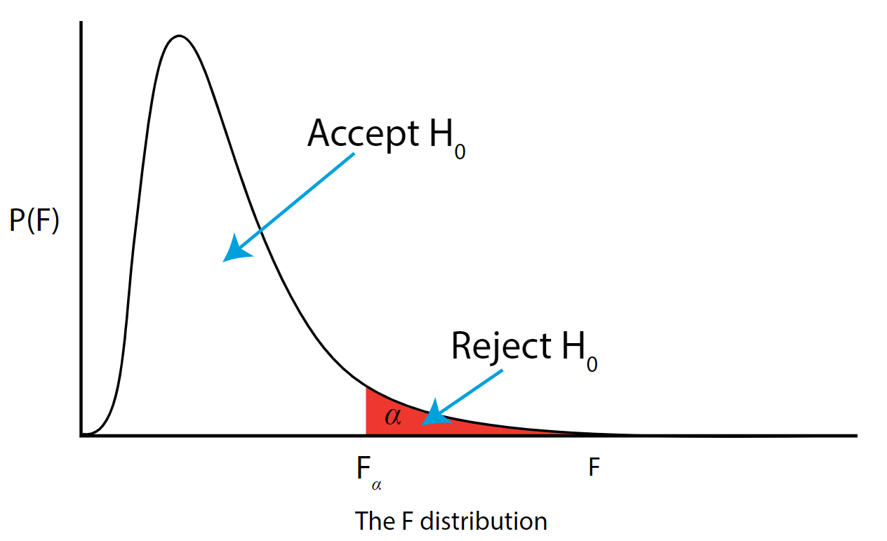.png?revision=1&size=bestfit&width=629&height=383 "steps in hypothesis testing using z test")
Step 7: Based on steps 5 and 6, draw a conclusion about H0
If the \(F_{\text{\calculated}}\) from the data is larger than the \(F_{\alpha}\), then you are in the rejection region and you can reject the null hypothesis with \((1 - \alpha)\) level of confidence.
Note that modern statistical software condenses steps 6 and 7 by providing a \(p\)-value. The \(p\)-value here is the probability of getting an \(F_{\text{calculated}}\) even greater than what you observe assuming the null hypothesis is true. If by chance, the \(F_{\text{calculated}} = F_{\alpha}\), then the \(p\)-value would exactly equal \(\alpha\). With larger \(F_{\text{calculated}}\) values, we move further into the rejection region and the \(p\) - value becomes less than \(\alpha\). So the decision rule is as follows:
If the \(p\) - value obtained from the ANOVA is less than \(\alpha\), then reject \(H_{0}\) and accept \(H_{A}\).
If you are not familiar with this material, we suggest that you review course materials from your basic statistics course.
IMAGES
VIDEO
COMMENTS
Related posts: Null Hypothesis: Definition, Rejecting & Examples and Understanding Significance Levels. Two-Sample Z Test Hypotheses. Null hypothesis (H 0): Two population means are equal (µ 1 = µ 2).; Alternative hypothesis (H A): Two population means are not equal (µ 1 ≠ µ 2).; Again, when the p-value is less than or equal to your significance level, reject the null hypothesis.
A Z-test is a type of statistical hypothesis test where the test-statistic follows a normal distribution. The name Z-test comes from the Z-score of the normal distribution. This is a measure of how many standard deviations away a raw score or sample statistics is from the populations' mean. Z-tests are the most common statistical tests ...
Conduct a hypothesis test using a z-score statistics, locating critical region, and make a statistical decision including. Explain the purpose of measuring effect size and power, and be able to compute Cohen's d. Exercises - Ch. 10. List the main steps for hypothesis testing with the z-statistic. When and why do you calculate an effect size?
Set this number aside for a moment. Step 3: Insert the numbers from Step 1 and Step 2 into the test statistic formula: Solving the formula, we get: Z = 8.99. We need to find out if the z-score falls into the " rejection region .". Step 4: Find the z-score associated with α/2. I'll use the following table of known values:
This Z-test calculator is a tool that helps you perform a one-sample Z-test on the population's mean. Two forms of this test - a two-tailed Z-test and a one-tailed Z-tests - exist, and can be used depending on your needs. You can also choose whether the calculator should determine the p-value from Z-test or you'd rather use the critical value ...
There are 5 main steps in hypothesis testing: State your research hypothesis as a null hypothesis and alternate hypothesis (H o) and (H a or H 1 ). Collect data in a way designed to test the hypothesis. Perform an appropriate statistical test. Decide whether to reject or fail to reject your null hypothesis. Present the findings in your results ...
Below these are summarized into six such steps to conducting a test of a hypothesis. Set up the hypotheses and check conditions: Each hypothesis test includes two hypotheses about the population. One is the null hypothesis, notated as H 0, which is a statement of a particular parameter value. This hypothesis is assumed to be true until there is ...
The Z-test January 9, 2021 Contents Example 1: (one tailed z-test) Example 2: (two tailed z-test) Questions Answers The z-test is a hypothesis test to determine if a single observed mean is signi cantly di erent (or greater or less than) the mean under the null hypothesis, hypwhen you know the standard deviation of the population.
Testin ggyp ( p) Hypotheses (6 Steps) 4. Determine critical values or cutoffs How extreme must our data be to reject the null? Critical Values: Test statistic values beyond which we will reject the null hypothesis (cutoffs) p levels (α): Probabilities used to determine the critical value 5. Calculate test statistic (e.g., z statistic)
There are several statistical tests for different types of distributions, usually, for a normal distribution, the z-test or test based on z-scores is used. Make a decision : Given the result obtained by the statistical test and the criteria for the decision defined in step 2, whether the null hypothesis is rejected or retained is determined.
the simplest hypothesis test, the z test. We learn how the z distribution and the z test make fair comparisons possible through standardization. Specifically, we learn: 1. How to use a z table. 2. How to implement the basic steps of hypothesis testing. 3. How to conduct a z test to compare a single sample to a known population. The z Table
The z test formula compares the z statistic with the z critical value to test whether there is a difference in the means of two populations. In hypothesis testing, the z critical value divides the distribution graph into the acceptance and the rejection regions.If the test statistic falls in the rejection region then the null hypothesis can be rejected otherwise it cannot be rejected.
Figure 8.1.1 8.1. 1: You can use a hypothesis test to decide if a dog breeder's claim that every Dalmatian has 35 spots is statistically sound. (Credit: Robert Neff) A statistician will make a decision about these claims. This process is called "hypothesis testing." A hypothesis test involves collecting data from a sample and evaluating the data.
Next step to to check if we can use the z-test for this hypothesis testing. Normal distribution of data : Test of normality is found ok; All data points are independent: Yes independent samples are considered. Standard deviation is known : Yes, value is given in problem statement; Sample Size ≥ 30 : yes
The goal of hypothesis testing is to determine the likelihood that a population parameter, such as the mean, is likely to be true. In this section, we describe the four steps of hypothesis testing that were briefly introduced in Section 8.1: Step 1: State the hypotheses. Step 2: Set the criteria for a decision. Step 3: Compute the test ...
This chapter lays out the basic logic and process of hypothesis testing. We will perform z tests, which use the z score formula from Chapter 6 and data from a sample mean to make an inference about a population.. Logic and Purpose of Hypothesis Testing. A hypothesis is a prediction that is tested in a research study. The statistician R. A. Fisher explained the concept of hypothesis testing ...
6 Hypothesis Testing: the z-test. We've all had the experience of standing at a crosswalk waiting staring at a pedestrian traffic light showing the little red man. You're waiting for the little green man so you can cross. After a little while you're still waiting and there aren't any cars around. You might think 'this light is really ...
Using this information with the generic form, which mimics a t t test statistic, the proportions test statistic is. ztest = p^ − p pq n−−√ (9.5.3) (9.5.3) z t e s t = p ^ − p p q n. where p p is the number k k which appears in the H0 H 0 hypothesis statement (see table above). This test statistic is valid only if np ≥ 5 n p ≥ 5 ...
Z-tests are statistical hypothesis testing techniques that are used to determine whether the null hypothesis relating to comparing sample means or proportions with that of population at a given significance level can be rejected or otherwise based on the z-statistics or z-score. As a data scientist, you must get a good understanding of the z-tests and its applications to test the hypothesis ...
Step 7: Based on Steps 5 and 6, draw a conclusion about H 0. If F calculated is larger than F α, then you are in the rejection region and you can reject the null hypothesis with ( 1 − α) level of confidence. Note that modern statistical software condenses Steps 6 and 7 by providing a p -value. The p -value here is the probability of getting ...
An area of .05 is equal to a z-score of 1.645. Step 6: Find the test statistic using this formula: For this set of data: z= (112.5 - 100) / (15/√30) = 4.56. Step 6: If Step 6 is greater than Step 5, reject the null hypothesis. If it's less than Step 5, you cannot reject the null hypothesis.
Hypothesis testing is a way to validate the claim of an experiment. ... Steps to perform Z-test: First, identify the null and alternate hypotheses. Determine the level of significance (∝). Find the critical value of z in the z-test using; Calculate the z-test statistics. Below is the formula for calculating the z-test statistics.
Step 7: Based on steps 5 and 6, draw a conclusion about H0. If the F\calculated F \calculated from the data is larger than the Fα F α, then you are in the rejection region and you can reject the null hypothesis with (1 − α) ( 1 − α) level of confidence. Note that modern statistical software condenses steps 6 and 7 by providing a p p -value.