ozone depletion introduction for essay

Talk to our experts

1800-120-456-456

Depletion of Ozone Layer Essay

Essay on Depletion of Ozone Layer

The essay on ozone layer depletion and protection gives us insight into changes in our environment. Ozone is super-charged oxygen in the lower level of the stratosphere. It makes a layer in the air, which goes about as a spread to the Earth against the bright radiation of the Sun. The ozone layer's shelter is with a variable degree less thick close to the outside of the Earth contrasted with the tallness of 30km. This depletion of Ozone layer essay explains the causes and effects of its depletion.

Ozone Layer Depletion

Ozone layer consumption is the diminishing of the ozone layer present in the upper air. This happens when the chlorine and bromine iotas in the environment interact with ozone and crush the ozone atoms. One chlorine can pulverize 100,000 atoms of ozone. It is devastated more rapidly than it is made. A few mixes discharge chlorine and bromine on presentation to high bright light, which at that point adds to the ozone layer consumption. Such mixes are known as Ozone Depleting Substances.

This essay on ozone layer in English states the most important causes of ozone depletion. A few contaminations in the environment like chlorofluorocarbons (CH 3 ) cause the exhaustion of the ozone layer. These CFCs and other comparable gases, when reaching the stratosphere they are separated by the bright radiation, and accordingly, the free particles of chlorine or bromine. These molecules are profoundly responsive to ozone and disturb stratospheric science. The responses drain the ozone layer. Researchers state that the unregulated dispatching of rockets brings about substantially more exhaustion of the ozone layer than the CFCs do. If not controlled, this may bring about a tremendous loss of the ozone layer constantly by 2050.

The depletion of ozone layer essay also provides the following effects of the depletion. Because of the consumption of the ozone layer, the Earth is presented to ultra-disregard radiation. These beams cause a harmful impact on living creatures on the Earth. It influences the cycle of photosynthesis in plants. Ascend in the temperature, different skin infections, a decline of invulnerability, and so forth are the plausible outcomes. Direct presentation to bright radiations prompts skin and eye malignant growth in creatures. Tiny fishes are incredibly influenced by the introduction to destructive bright beams. These are higher in the amphibian natural way of life.

The greater part of the cleaning items has chlorine and bromine, delivering synthetics that discover a route into the air and influence the ozone layer. These ought to be subbed with common items to secure the climate. The vehicles produce a lot of ozone-depleting substances that lead to a dangerous atmospheric deviation, just as ozone consumption. Along these lines, vehicles' utilization ought to be limited, however much as could be expected. Normal techniques ought to be actualized to dispose of bugs and weeds as opposed to utilizing synthetics. One can utilize eco-accommodating synthetic compounds to eliminate the nuisances or eliminate the weeds physically.

For the security of the ozone layer, the Vienna Conference in March 1985 was held. In September 1987, the Montreal Protocol was agreed upon. This was followed by the Kyoto Protocol of 1997. Under the Protocol, 37 nations invest in a decrease of four GreenHouse Gases and two gatherings of gases delivered by them, and all part nations give general responsibilities.

Prevention of the Depletion of the Ozone Layer

Ozone layer depletion can be avoided by first understanding the root of the problem. This means that first, the students have to understand what causes ozone layer depletion and then reduce those practices as much as possible. One of the reasons why ozone depletion happens is because of the increased production of chlorofluorocarbons. These are present in many things around us such as in solvents, refrigerators, air conditioners, etc.

The ozone layer also gets depleted due to Nitrogenous compounds such as NO 2 , NO, N 2 O. One other reason for ozone layer depletion are the natural causes or processes such as Sun-spots etc but this cannot be considered as one of the main reasons for the depletion in the Ozone layer because the only harm it does is 1-2 percent. Some other examples of the things which deplete the Ozone layer are natural volcanoes. So, the methods to prevent Ozone layer Depletion are avoiding the use of Ozone-depleting substances which include, CFCs in refrigerators etc or avoiding using private means of transport and using public transports as much as possible or trying using bicycle or walking which is an environmentally friendly solution. Also, the students should note that replacing eco-friendly substances at the place of chlorine, bromine or other harmful releasing products helps in the prevention of ozone layer depletion.

The essay on depletion of the ozone layer tells us about the harmful effects of it and ways to combat it. This ozone layer depletion essay in English helps us recognize its cause and provides us with insight into how to stop them.

FAQs on Depletion of Ozone Layer Essay

1. What is the Ozone Layer?

Ozone has been the most receptive type of sub-atomic oxygen and the fourth most impressive oxidizing specialist. It has a wonderful focus at around 2 ppm or less. However, higher fixation is aggravating. It is utilized as a disinfectant and blanching operator. In nature, O 3 is framed in the stratosphere when bright light strikes an oxygen particle. A photon parts the oxygen particle into two profoundly receptive oxygen atoms(O). These consolidate rapidly with an oxygen particle to shape ozone. The O 3 promptly retains UV light and separates into its constituent segments.

2. Where is the Ozone Hole found?

One instance of ozone depletion is the yearly ozone hole over Antarctica that has been continuously on-going during the Antarctic spring, since the mid-1980s. This isn't generally a gap through the ozone layer, yet rather a huge territory of the stratosphere with incredibly low ozone measures. Understand that ozone exhaustion isn't restricted to the zone over the South Pole. Exploration has indicated that ozone consumption happens over the scopes that incorporate North America, Europe, Asia, and quite a bit of Africa, Australia, and South America. In the 19th century, the ozone hole has extended to every continent.

3. Where can I find a well-written essay on the Depletion of the Ozone Layer?

Students can easily find a well-written essay on the Depletion of the Ozone layer at Vedantu. The essay is informative and easy to understand because of the proper usage of simple words. There are various other essays available also in the Vedantu app which are easily available to the students for their better preparation for any examinations or competitions which they may be expecting. To find more such essays sign in at Vedantu via our website or app and read an essay of your choice.

4. Are there any harmful effects due to the Depletion of the Ozone layer?

There are numerous harmful effects of Ozone layer depletion. Some of them are increased temperature of the planet earth, variants of skin infections, eye problems, a faster rate of aging, Cancer, reduction in the rate of flowering plants and so much more. The students must know that it is very important to avoid this from happening or the results will be disastrous. Hence, they must educate themselves by learning about the causes of these effects and how to reduce them for a better world.

5. Why should I study the Depletion of the Ozone layer?

The students should know about the study of the Ozone layer as this is what affects the climate indirectly and directly. One must take the appropriate measures to do everything they possibly can in order to make sure that they are doing their due for the climate and the planet earth. There should be various meetings, events and other group-based activities which educate people about the importance of the Ozone layer and why its depletion should be avoided at all costs. The students should also take the matters into their own hands to make sure that the people around them are not causing any excessive damage or adding to the reasons for the depletion of the ozone layer. This can only be made sure if the institutions educate the students on the various environmental topics and how the students can make a difference. Teachers and schools are also responsible in many ways to present the students with these topics which are later on helpful in life. This is why it is important for the essays in English to be about the various informative things which are needed in real life. Thus, it is important that every student understands the essay about the depletion of the ozone layer as it not only helps them to write in English smoothly but also makes sure they are getting educated through the various topics aforementioned. Thus, make sure that you read the essay on the depletion of the ozone layer as it is not only a theoretical scientific topic but also helps in enhancing one’s writing skills.

Report Highlights
EU-Summaries

About the publications

The evolution of ozone layer depletion, its impact on climate change, health and the environment.

Level 1: Highlights [en]
Level 2: Long Summary [en]

Introduction

The Assessment reports on key findings on environment and health since the last full Assessment of 2010, paying attention to the interactions between ozone depletion and climate change .

The most severe and most surprising ozone loss was discovered to be recurring in springtime over Antarctica. The loss in this region is commonly called the “ozone hole” because the ozone depletion is so large and localized. In response to the prospect of increasing ozone depletion, the governments of the world crafted the 1987 United Nations Montreal Protocol as an international means to address this global issue. Thanks to development of “ozone-friendly” substitutes for the now-controlled “Ozone Depleting Substances” (ODS) substances, such as chloro-fluoro-carbons or CFCs long used a.o. in most refrigeration and air conditioning systems, the total global accumulation of ODS has slowed and begun to decrease and initial signs of recovery of the ozone layer have been identified. Production and consumption of all principal ODS by developed and developing nations has already been largely decreased and will be almost completely phased out before the middle of the 21 st century.

Those gases that are still increasing in the atmosphere , such as halon-1301 and HCFCs, will begin to decrease in the coming decades if compliance with the Protocol continues. However, it is only after mid-century that the effective abundance of ODS is expected to fall to values that were present before the Antarctic ozone hole was first observed in the early 1980s.

According to the UNEP progress report (2015) 1 , by 2013 the implementation of the Montreal Protocol had already achieved significant benefits for the ozone layer and, consequently, for surface UV-B radiation . Model calculations have shown that, without the Montreal Protocol, a deep Arctic “ ozone hole”, would have occurred in 2011 given the meteorological conditions in that year. The decline of stratospheric ozone over the Northern Hemisphere mid-latitudes would have continued, more than doubling to about 15% by 2013 relative to the onset of ozone-depletion. In addition, the Antarctic ozone hole would have been 40% larger in 2013 relative to what was observed, with enhanced loss of ozone also at sub-polar latitudes of the Southern Hemisphere.

1 UNITED NATIONS ENVIRONMENT PROGRAMME Environmental Effects of Ozone Depletion and its Interactions with Climate Change Progress Report, 2015

What is stratospheric ozone and how is it formed?

Ozone is constituted of three atom of oxygen combined which is formed in upper part of the Earth’s atmosphere in small amounts where it forms a layer. This layer is vital to human well-being and ecosystem health as it absorbs a large part of the Sun’s biologically harmful ultraviolet radiation .. This region, called the stratosphere , is more than 10 km (6 miles) above Earth’s surface. There, about 90% of atmospheric ozone is contained in the “ ozone layer ,” which shields us from harmful ultraviolet radiation from the Sun. In the mid-1970s, it was discovered that some human-produced chemicals could lead to depletion of the ozone layer.

By contrast, ozone formed at Earth’s surface in excess of natural amounts is considered “bad” ozone because it is harmful to humans, plants, and animals but ozone produced naturally near the surface and in the lower atmosphere plays an important beneficial role in chemically removing pollutants from the atmosphere.

The distribution of total ozone over Earth varies with location on timescales that range from daily to seasonal. Total ozone is generally lowest at the equator where it is produced and highest in polar region atmosphere . The variations are caused by large-scale movements of stratospheric air and the chemical production and destruction of ozone. An important feature of seasonal ozone changes is the natural chemical destruction that occurs when daylight is continuous in the summer polar stratosphere , which causes total ozone to decrease gradually toward its lowest values in early fall.

How is stratospheric ozone depleted?

The initial step in the depletion of stratospheric ozone induced by human activities is the emission, at Earth’s surface, of certain organic gases containing chlorine and bromine like the CFCs used in part because their low reactivity and toxicity along with carbon tetrachloride (CCl 4 ) and methyl chloroform (CH 3 CCl 3 ) and the halons, which were used in fire extinguishers. Halogen source gases are compared in their effectiveness to destroy stratospheric ozone using their Ozone Depletion Potential (ODP) calculated relative to CFC-11, which has an ODP defined to be 1. A gas with a larger ODP destroys more ozone over its atmospheric lifetime. Lifetimes of the principal zone-depleting substances vary from 1 to 100 years.

Because they are unreactive and do not dissolve readily in rain or snow, these gases accumulate in the lower atmosphere . Natural air motions transport these accumulated gases to the stratosphere , where they are converted to more reactive molecules by the ultraviolet radiation originating from the sun. Some of these molecules, like chlorine radicals and chlorine monoxide (ClO) then participate in reactions that destroy ozone in “catalytic” cycles made up of two or more separate reactions. As a result, a single chlorine or bromine atom can destroy many thousands of ozone molecules before it leaves the stratosphere and returns to the lower atmosphere where these reactive chlorine and bromine gases are removed from Earth’s atmosphere by rain and snow.

The severe depletion of the Antarctic ozone layer known as the “ ozone hole” occurs because of the special meteorological and chemical conditions that exist there when the very low winter temperatures in the Antarctic stratosphere cause polar stratospheric clouds (PSCs) to form which are isolated from stratospheric air in the polar vortex and preventing “fresh ozone” from the tropical region to temporarily replace the destroyed ozone, thus producing the ozone hole in Antarctic springtime. Depletion of the global ozone layer increased gradually in the 1980s and reached a maximum of about 5% in the early 1990s. The depletion has lessened since then and now is about 3% averaged over the globe.

Significant depletion of the Arctic ozone layer also occurs in most years in the late winter/early spring period (January–March). However, the maximum depletion is less severe than that observed in the Antarctic and with large year-to-year differences as a consequence of the highly variable meteorological conditions found in the Arctic polar stratosphere .

Eventually other factors such as changes in solar radiation , as well as the formation of stratospheric particles after volcanic eruptions, also influence and may affect the ozone layer .

Was the Montreal protocol signed in 1985 effective to protect and restore the ozone layer?

The Montreal Protocol controls led to a substantial reduction in the emissions of ODS over the last two decades. The Scientific Assessment Panel of the Montreal Protocol on Substances that Deplete the Ozone Layer 2 concludes that atmospheric abundance of most controlled ODS is decreasing. There are several indications that the global ozone layer is beginning to recover from ODS-induced depletion.

Observations now show a clear 5% increase of ozone in the upper stratosphere (42 km) over the 2000-2013 period. Model simulations suggest that about half of this increase results from a cooling in this region due to CO 2 increases, while the other half results from Equivalent Effective Stratospheric Chlorine (EESC), designed as one measure of the potential for ozone depletion in the stratosphere, decreases. However, the variability of the atmosphere and the influence of climate change have hindered a definitive attribution of the observed global ozone increases since 2000 to the concomitant ODS decreases.

In Antarctica, large ozone depletion continues to occur each year. In the Arctic, ozone depletion is generally less pronounced than in Antarctica but more variable: the very high stratospheric ozone concentrations observed in the spring of 2010 were followed by record-low concentrations in spring 2011.

These reductions of emissions of ODS, while protecting the ozone layer , have the additional and very significant benefit of reducing the human contribution to climate change . Without Montreal Protocol controls, the contribution to climate forcing from annual ODS emissions could now be 10-fold larger than its present value, which would be a significant fraction of the climate forcing from current carbon dioxide (CO 2 ) emissions 3 . Increases in ODS substitute gases, which are also greenhouse gases but to a lesser extent, could offset much of this climate benefit by substantially contributing to human induced climate forcing in the coming decades.

What about the increase of UV-B irradiance associated to the ozone layer depletion?

As a result of the success of the Montreal Protocol in limiting ozone depletion, since the mid-1990s the changes in UV-B measured at many sites are due largely to factors other than ozone. Nevertheless stabilisation of the concentrations of stratospheric ozone and possible beginning of a recovery of UV-B irradiance are not yet detectable in the measurements because of the large natural variability.

In the meantime, the increases in UV-B irradiance, ranging from 5 to 10% per decade and reported for several northern mid-latitude sites, are caused predominantly by reductions in cloudiness and aerosols while UV-B irradiance decrease at some northern high latitude sites, during that period, are mainly due to reduction in snow- or ice-cover. Future levels of UV-B irradiance at high latitudes will be determined by the recovery of stratospheric ozone and by changes in clouds and reflectivity of the Earth’s surface. In Antarctica, reductions of up to 40% in mean noontime UV Index (UVI) are projected for 2100.

According to the progress report 2015, measurements at several sites over the last decade have shown decreases in surface UV-B radiation that are consistent with observed increases in total ozone . However, at some sites, changes in aerosols , clouds and, at high latitudes, sea ice were the main drivers of changes in UV-B radiation.

The UVI is indeed, according to the UNEP report, projected to decrease by up to 7% at northern high latitudes because of the anticipated increases in cloud cover and reductions in surface reflectivity due to ice-melt while anticipated decreases in aerosols would result in increases in the UVI, particularly in densely populated areas. Outside the Polar regions, future changes in UV-B irradiance will likely be dominated by changes in factors other than ozone and by the end of the 21 st century, the effect of the recovery of ozone on UV-B irradiance will be very small, leading to decreases in UVI of between 0 and 5%.

The 2015 report states that from a variety of proxy data for nine locations in Spain, erythremal irradiance increased between 1950 and 2011 by about 13%, of which half was due to decreases in ozone while between 1985 and 2011, an increase of about 6% was calculated, mostly due to decreasing amounts of aerosols and clouds.

In the Arctic, the areal extent and thickness of sea ice continue to decline. Recent modelling efforts estimate that exposure to the UV-B wavelength range in the surface waters of the Arctic Sea may increase as much as tenfold between 1950 and 2100 due to the melting of sea ice.

What is the link between the ozone layer depletion and climate change?

Ozone depletion itself is not the principal cause of global climate change . Changes in ozone and climate are directly linked because ozone absorbs solar radiation and is also a greenhouse gas . Stratospheric ozone depletion leads to surface cooling, while the observed increases in tropospheric ozone and other greenhouse gases lead to surface warming.

The ozone layer depletion also helped to keep East Antarctica cold, but conversely has helped to make the Maritime Antarctic region one of the fastest warming regions on the planet. In contrast to the warming of most ocean waters, there is a significant cooling in the North Atlantic between Greenland and Ireland. This is due to a weakening of the Gulf Stream that heats the North Atlantic, the American East coast , and Northern Europe.

For the 2015 report, when considering the effects of climate change , it has become clear that processes resulting in changes in stratospheric ozone are more complex than previously believed. As a result of this, human health and environmental problems will be longer-lasting and more regionally variable.

The solar UV radiation has the potential to contribute to climate change via its stimulation of emissions of carbon monoxide , carbon dioxide , methane , and other volatile organic compounds from plants, plant litter and soil surfaces but their magnitude, rates and spatial patterns remain highly uncertain at present.

These UV radiation processes could also increase emissions of trace gases that affect the atmospheric radiation budget ( radiative forcing ) and hence changes in climate.

Resultant changes in precipitation patterns have been correlated with ecosystem changes such as increased tree growth in Eastern New Zealand and expansion of agriculture in South-eastern South America. Conversely, in Patagonia and East Antarctica, declining tree and moss bed growth have been linked to reduced availability of water. A full understanding of the effects of ozone depletion on terrestrial ecosystems in these regions should therefore consider both UV radiation and climate change .

Solar UV radiation is driving production of substantial amounts of carbon dioxide from Arctic waters. The production is enhanced by the changes in rainfall, melting of ice, snow and the permafrost , which lead to more organic material being washed from the land in to Arctic rivers, lakes and coastal oceans. Solar UV radiation degrades this organic material, which stimulates CO 2 and CO emissions from the water bodies, both directly and by enhanced microbial decomposition. New results indicate that up to 40% of the emissions of CO 2 from the Arctic may come from this source, much larger than earlier estimates.

Where photochemical priming plays an important role, changes in continental runoff and ice melting, due to climate change , are likely to result in enhanced UV-induced and microbial degradation of dissolved organic matter and release of carbon dioxide (CO 2 ). Such positive feedbacks are particularly pronounced in the Arctic resulting in Arctic amplification of the release of CO 2 (see next point).

Other changes in climate associated with ozone layer depletion include changes to wind patterns , temperature and precipitation across the Southern Hemisphere. More intense winds lead to enhanced wind-driven upwelling of carbon-rich deep water and less uptake of atmospheric CO 2 by the Southern Ocean , reducing the oceans potential to act as a carbon sink (less sequestering of carbon). These winds also transport more dust from drying areas of South America into the oceans and onto the Antarctic continent. In the oceans this can enhance iron fertilisation resulting in more plankton and increased numbers of krill . On the continent the dust may contain spores of novel microbes that increase the risk of invasion of non-indigenous species and this transport from drying areas, such as in South America, into the oceans, may enhance fertilisation by iron and resulting in more plankton and greater carbon uptake.

Conversely, says the 2015 report, climate change could enhance the production in marine environments of short-lived halogens (e.g., methylene chloride, bromoform) that cause depletion of ozone in the stratosphere and troposphere .

What is the link between ozone depletion gases (ODS) and climate change?

Global average abundances of the major, well-mixed, long-lived greenhouse gases

Most ozone depleting substances are also strong greenhouse gases and, in a world without the Montreal Protocol on ODS ban (minus 98% consumption worldwide between 1986 and 2015) restrictions, annual ODS emissions could be today as important for climate forcing as those of CO 2 and be 10-fold larger than its present value 4 . Transitory ODS substitute gases, H-CFCs first, then HFCs (hydrofluorocarbons) are also greenhouse gases but most of them to a lesser extent and their transitory use as substitutes to ODS represented the most important contribution to the reduction of the global greenhouse gases emissions.

Anyway, because the first generations of substitute chemicals, like hydrofluorocarbons (F-gases or HFCs) had still a significant greenhouse gas potential which could in the long term offset the climate benefit by substantially contributing to human induced climate forcing, their progressive phasing out was decided in 2016 in an amendment of the Montreal Protocol 5 .

Other changes in climate associated with ozone layer depletion include changes to wind patterns, temperature and precipitation across the Southern Hemisphere reducing the oceans potential to act as a carbon sink (less sequestering of carbon).

Has ozone depletion produced significant effects on human health?

In spring 2011 the erythemal (sunburning) dose averaged over the duration of the low- ozone period increased by 40-50% at several Arctic and Scandinavian sites in response to episodic decreases of ozone at high latitudes (about 25% over Central Europe). Nevertheless, according to the UNEP report (2014), changing behaviour with regard to sun exposure by many fair-skinned populations has probably had more significant adverse and beneficial consequences on human health than increasing UV-B irradiance due to ozone depletion. The increase in holiday travel to sunny climates, wearing clothing that covers less of the body, and the desire for a tan are all likely to have contributed to higher personal levels of exposure to UV-B radiation than in previous decades.

Regarding adverse effects:

Immediate adverse effects of excessive UV-B irradiation are sunburn of the skin and inflammation of the eye including photo- conjunctivitis or photo-keratitis, cancers of the eyelid and the surface of the eye, cortical cataract and pterygium.
Long-term regular low dose or repeated high-dose exposure to the sun causes melanoma and non-melanoma (basal and squamous cell ) carcinomas of the skin and cataract and pterygium (a growth on the conjunctiva ) of the eye.

The incidence of each of these skin cancers has risen significantly since the 1960s in fair-skinned populations , but has stabilised in recent years in younger age groups in several countries, perhaps due to effective public health campaigns. Cataract is the leading cause of blindness worldwide. The 2015 report underlines that incidence of both non- melanoma skin cancers, primarily in fair-skinned populations, and cutaneous melanoma (CM) continues to increase globally with exposure to solar UV radiation the most important cause but, in many countries, mortality may have peaked. For example, the age-standardised incidence rate of CM per 100,000 persons in the UK for 2009-2011 increased by 57% in men and 39% in women respectively, compared to 2000-2002 and doubled from 1982 to 2011 in the USA.

Exposure to solar UV radiation can also alter the immune response to a variety of microorganisms in animal studies, and recent reports support a similar role in humans.

Common strategies to avoid over-exposure to solar UV radiation should aim to balance the harmful and beneficial effects of sun exposure even if such a balance may be difficult to achieve in practice as the recommended time outdoors will differ between individuals, depending on personal factors such as skin colour, age, and clothing as well as on environmental factors such as location, time of day, and season of year.

Regarding beneficial effects of exposure of the skin to solar UV radiation the major known is the synthesis of vitamin D with is critical in maintaining blood calcium levels and is required for strong bones and its deficiency might increase the risk of an array of diseases such as cancers , autoimmune diseases and infections.

What are the impacts of ozone layer depletion and UV-B increases on terrestrial ecosystems?

Various abiotic and biotic factors affect plants are influenced by UV-B radiation in ways that can have both positive and negative consequences on plant productivity and functioning of ecosystem in intricate feedbacks and complexity. Plant productivity is likely decreased slightly due to the increased UV radiation while exposure to UV-B radiation can promote plant hardiness, and enhance plant resistance to herbivores and pathogens , improving the quality, and increase or decrease the yields of agricultural and horticultural products.

While UV-B radiation does not penetrate into soil to any significant depth, it can affect a number of belowground processes through alterations in aboveground plant parts, microorganisms , and plant litter . These include modifications of the interactions between plant roots, microbes, soil animals and neighbouring plants, with potential consequences for soil fertility , carbon storage, plant productivity and species composition. UV-B radiation can also influence rates of photodecomposition of dead plant and is now being considered as an important driver of decomposition, although uncertainty exists in quantifying its significance. It is known that UV radiation facilitates the breakdown of pesticides and may in some cases increase toxicity of certain pesticides and/or their degradation products.

The 2015 report also underlines that stimulation by UV radiation of polyphenolics can increase the nutritional quality of plant products and plant tolerance to stress conditions and that the increased frequency and extent of wildfires due to climate change become important sources of aerosols which emit black carbon (BC) and organic carbon (OC) smoke particles that can persist in the atmosphere for days to weeks with significant effects on surface UV radiation.

What are the impacts of ozone layer depletion on aquatic ecosystems?

Species composition and distribution of many marine ecosystems may strongly be influenced with warmer oceans due to feedbacks between temperature, UV radiation and greenhouse gas concentrations.

Higher air temperatures are increasing the surface water temperatures of numerous lakes and oceans, with many large lakes warming at twice the rate of air temperatures in some regions. Warming of the ocean results in stronger stratification that decreases the depth of the upper mixed layer and also reduces upward transport of nutrients across the thermocline from deeper layers. The decrease in the depth of the upper mixed layer exposes organisms that dwell in it to greater amounts of solar visible and UV radiation which may overwhelm their capability for protection and repair by producing UV-absorbing compounds. On the other hand, climate change -induced increases in concentrations of dissolved organic matter in inland and coastal waters reduce the depth of penetration of UV radiation.

Increased concentrations of atmospheric CO 2 are continuing to cause acidification of the ocean , which also alters marine chemical environments and interferes with the calcification process by which organisms, such as phytoplankton, macroalgae and many animals including molluscs , zooplankton and corals, produce exoskeletons protecting themselves from predators and solar UV radiation .

Phytoplankton (primary feed producers) are decreasing along the West side of the Antarctic Peninsula due to increased solar UV-B radiation and rapid regional climate change . For others such as corals, the warming may alter their tolerance of other stressors. This warming also can shift the thermal niche of organisms towards the pole and causes changes in community structure. Change in ice phenology as well as light and nutrient availability may affect species composition.

Decreased penetration of UV radiation also reduces the natural disinfection of surface water containing viruses , pathogens , and parasites. In contrast to the UV-disinfection of surface waters , exposure to high levels of UV radiation can either stress or suppress the immune system of hosts, making them more susceptible to infection.

Eventually, microplastics debris created in the oceans by solar UV radiation from the weathering of plastic litter on beaches is also a growing environmental issue. These microplastic particles concentrate toxic chemicals dissolved in seawater and are ingested by zooplankton, thus providing a potential mechanism for transfer of pollutants into the marine food web.

Are there other environmental effects of ozone layer depletion?

The carbon cycle is strongly influenced by interactions between droughts and intensity of UV- radiation at the Earth’s surface. Increased aridity due to climate change and severity of droughts will change the amount of plant cover, thereby increasing UV-induced decomposition of dead plant matter (plant litter ). These increased losses could have large impacts on terrestrial carbon cycling in arid ecosystems .

New results have shown that lignin is readily decomposed with exposure to solar UV radiation , reducing long-term storage of carbon in perennial terrestrial systems.

UV radiation also induces photoreactions that dissipate pollutants and pathogens says the 2015 report, which affect the fate and transport of pesticides , pharmaceuticals, heavy metals , nanomaterials and pathogens.

Is ozone layer depletion affecting air quality?

UV radiation is known to be a critical driver of the formation of photochemical smog, e.g. ozone and aerosols . UV radiation may also play a role in the destruction of aerosol particles. Ground-level ozone concentrations may increase substantially over large geographic regions due to a combination of stratospheric ozone recovery and climate change in the coming decades. UV radiation is an essential driver for the formation of photochemical smog, which consists mainly of ground-level ozone and particulate matter . Greater exposures to these pollutants have been linked to increased risks of cardiovascular and respiratory diseases in humans and are associated globally with several million premature deaths per year. Tropospheric (ground-level) ozone may alter biological diversity and affect the function of natural ecosystems and also have adverse effects on yields of crops. Future changes in UV radiation and climate and significant reductions in emissions will alter the rates of formation of ground-level ozone and some particulate matter and must be considered in predictions of air quality and consequences for human and environmental health.

Hydroxyl radicals (∙OH), which are responsible for the self-cleaning of the atmosphere UV radiation , are also affected by changes in UV radiation. However, on global scales, models differ in their predictions with consequent uncertainties.

By contrast, based on current data says the 2015 report, the amount of trifluoroacetic acid (TFA) formed from HCFCs and HFCs in the troposphere is too small to be a risk to the health of humans and the environment. No new negative environmental effects of the substitutes for the ozone depleting substances or their breakdown-products have been identified even if some present substitutes for the ozone depleting substances continue to contribute, although much less than former ozone depleting substances like CFCs, to global climate change if concentrations rise above current levels.

Has the increase of UV-radiation an impact on materials resistance?

Solar UV radiation and climate change affect the outdoor service lifetime of PVC building products, still the most-used plastic in building and of polypropylenes containing recycled plastic by changes in bulk morphology that also results in a reduced. Nanoscale inorganic fillers could provide superior stability against solar UV irradiation relative to conventional fillers in coatings especially those in clear-coatings on wood or textile fibre-coatings of textile and plastics. The benefits of nanofillers in bulk plastics, however need more information to assess their efficacy.

Regarding wood , graphene, zirconium dioxide, iron oxide, titanium, and cerium oxide can control UV-induced yellowing in several wood species . Similarly, surface modification of wood with nanocellulose crystals and epoxidised soybean oil also result in good UV stabilisation.

Effectiveness of specific fabrics depends on the weave characteristics but can be further improved by surface-treating the fibres with a UV absorber. Textile fabrics block the personal exposure to solar UV radiation , whereas glass usually blocks mainly UV-B radiation. Glazing for windows is being developed to further improve their thermal properties and also results in increased filtering of the UV radiation with benefits for health of humans and indoor components of buildings and artwork. In cable-jackets with the new aluminum-based fire retardants, initial degradation by UV radiation yields a filler-rich surface layer that screens the underlying polymer from further degradation.

What was the situation of ozone-depleting substances in the European Union market in 2015?

Consumption of controlled ozone–depleting substances

The European Environmental Agency (EEA) publishes a yearly report on the subject 6,7 . Globally, consumption of ODS controlled under the Montreal Protocol declined by some 98.34 % worldwide between 1986 and 2015.

However, much remains to be done to ensure that the damage to the ozone layer is reverted. Initiatives to further reduce releases of ODS could involve the following:

Addressing the strong growth in the production and consumption of HCFCs in developing countries;
Collecting and safely disposing of the large quantities of ODS contained in old equipment and buildings (the so-called ODS 'banks');
Ensuring that restrictions on ODS continue to be properly implemented and the remaining worldwide use of ODS declines further;
Preventing illegal trade in ODS; and
Strengthening the international and European framework on ODS (e.g. inclusion of other known ODS, restricting exemptions).

Consumption: The consumption of ODS in the EU has been negative or close to zero since 2010 and, in 2015, the consumption of controlled substances reached its lowest negative level since 2006 . Controlled substances with a high ODP (e.g. CFCs and CTC) exhibit a different trend in consumption from those with a low ODP (e.g. HCFCs).

Imports: The largest imported quantities were of hydrochlorofluorocarbons (HCFCs) (52 % when expressed in metric tonnes), methyl bromide (MB), chlorofluorocarbons (CFCs) and bromochloromethane (BCM) and virgin carbon tetrachloride (CTC) and virgin CFCs when expressed in ODP tonnes.

Exports: The quantity of controlled virgin substances exported from the EU (including re-export) continued to decline (down by 17 %), and the total quantity exported in 2015 (2 152 ODP tonnes) was made up predominantly of HCFCs (84 % when expressed in metric tonnes), 26 % lower than that in 2014.

Production: Controlled substances produced were predominantly HCFCs (71 % of the total production in metric tonnes), CTC and trichloroethane (TCA) down by 4 %. Controlled substances were produced almost exclusively for feedstock use inside the EU (91 % of the quantity produced, in metric tonnes) with a decline in production for some uses, e.g. refrigeration, unintentional by-production, process agent use and feedstock use outside the EU.

Only minor quantities of CFCs and hydrobromofluorocarbons (HBFCs), and no MB or BCM, were produced in 2015. A total of about 10 000 tonnes of controlled substances (CTC, HCFCs and CFCs) were destroyed, explained to a large extent by the increased destruction, compared with 2014, of unintentionally produced CTC.

The production of new substances (expressed in metric tonnes) was six times higher than the production of controlled substances. However, owing to the lower ODP of new substances, these amounts constitute, when expressed in ODP tonnes, approximately 30 % of the combined production of controlled and new substances in the EU.

Emissions: The total make-up and emissions of controlled substances used as process agents stayed well below restrictions imposed by both the Montreal Protocol and the ODS Regulation. Emissions of controlled substances from their use as feedstock decreased to an average emissions rate of 0.07 % (calculated as the ratio of total emissions to total quantities used as make-up (4), expressed in metric tonnes).

F-gases: Approximately 75 % (both in tonnes and CO 2 eq.) of F-gases supplied to the market in 2015 were intended for use as refrigerants for refrigeration, air conditioning and heating purposes. These were almost exclusively HFCs.

Of 2015 total supply, 10 % (by mass) was intended for use in insulation foams; 96 % of this was HFCs. Measured in CO 2 eq., the proportion of F-gases intended for use in foams was only 3 %.
Aerosols (both medical and non-medical) were the intended application of 10 % (tonnes) of 2014 total supply, 6 % as CO 2 eq. The gases used for aerosols were almost entirely HFCs.
SF6 intended for electrical equipment (switchgear) contributed only a small fraction when measured in tonnes but a considerable portion of supply as CO 2 eq.

The overall trends that can be identified from companies reporting can be summarised as follows:

Production of F-gas continued to decline, with 2015 levels 5 % (as CO 2 eq.) below those reported for 2014;
Imports decreased by about 40 % compared with the exceptionally high amounts reported for 2014 (by weight and as CO 2 eq.). Compared with 2013, bulk imports in 2015 increased by about 8 % ;
Exports have decreased by 2 % (tonnes) or 1 % (CO 2 eq.) since 2014. Compared with 2013, exports in 2015 increased by 18 % (tonnes) and 23 % (CO 2 eq.).
Supply has decreased by about 24 % (by weight and as CO 2 eq.) since 2014. Compared with 2013, bulk supply (7) increased by 9 % by weight but decreased by 3 % as CO 2 eq. in 2015.

Destruction of F-gases has been increasing consistently since 2008, with the exception of very low numbers reported for 2013. While destroyed gases are not accounted for in the bulk supply/total supply metrics, if compared with bulk supply, the 2015 level of destruction would be 1.5 % of bulk supply by mass or 5 % as CO 2 eq.

Accidental poisoning
Acrylamide in food
Acupuncture
Agriculture
Aids Epidemic
Air Pollution Europe
Air quality in Europe
Allergenic fragrances
Aluminium exposure
Animal testing
Antibiotic resistance
Antibiotics Research
Antimicrobial resistance
Aquatic environment
Arctic Climate Change
Artificial Light
Artificial Light and Health
Aspartame Reevaluation
Aspirin & Cancer
Benzodiazepines
Biodiversity
Biological Diversity
Biosecurity
Bisphenol A
CO 2 Capture & Storage
Cancer rates and mortality, types and causes
Chemical Mixtures
Children & Screens
Chlorine Sodium Hypochlorite
Chlorpyrifos pesticide
Chronic Diseases on Labour Practices
Circular Economy
Climate Change
Climate Change Mitigation
Climate impact of shale gas
Climate impacts adaptation
Dental Amalgams
Dental Fillings
Desertification
Diet & Nutrition
Ecosystem Change
Effects of cannabis
Electromagnetic Fields
Electronic Cigarettes
Endocrine Disruptors
Endocrine disrupting properties of pesticides
Endocrine disruptors risks
Energy Saving Lamps
Energy Technologies
Epidemic diseases
Estrogen-progestogen cancer risk
Europe Green Deal
Evaluation of endocrine disruptors
Exposure to chemical mixtures
Fisheries and aquaculture
Fluorinated gases
Food & Agriculture
Food Wastage
Forests & Energy
Forests & agriculture land use
Fukushima Consequences
Fukushima accident
Genetically Modified Crops
Geothermal Energy
Global Biodiversity Outlook 4
Global Public Health Threats
Global Warming
Gluten intolerance
Glyphosate and cancer
Hazardous chemicals
Health Effects of Electromagnetic Fields
Health Environment Management
Illicit drugs in Europe
Impacts of a 4°C global warming
India Millennium Development Goals
Indonesian forests
Indoor Air Quality
Land Degradation and Desertification
Lyme Disease
Marine Litter
Marine litter
Mercury from dental amalgam
Mercury in CFL
Metal-on-Metal hip implants
Methylene glycol
Mineral extraction risks
Multiple vaccinations
Nano-silica
Nanomaterials
Nanotechnologies
Neonicotinoids
Nitrogen Dioxide
Non-human primates
Organic Food
Ozone layer depletion
Parabens used in cosmetics
Particulate Matter
Perfluorooctanoic acid (PFOA)
Personal Music Players & Hearing
Pesticides occupational risks
Pharmaceuticals environment
Phosphate resources
Phthalates Comparison
Phthalates in school supplies
Poly brominated flame retardant decaBDE
Power lines
Psychoactive Drugs
Radiological nuclear emergency
Respiratory Diseases
Safety of Cosmetics
Safety of sunscreens
Sand Extraction
Security Scanners
Silver Nanoparticles
Single-use plastics
Soils degradation
Solar Energy
State of the European Environment
Static Fields
Substitution of harmful chemicals
Sulfaxoflor Pesticide
Sunbeds & UV radiation
Sustainable oceans
Synthetic Biology
Thorium nuclear fuel
Tidal Energy
Titanium dioxide nanoparticles
Tooth Whiteners
Transgenic salmon
Tuberculosis
Wastewater management
Water Disinfectants
Water Resources
Water Resources Assessments
Water resources
Wind Resources
X-Ray Full-Body Scanners

Get involved!

This summary is free and ad-free, as is all of our content. You can help us remain free and independant as well as to develop new ways to communicate science by becoming a Patron!

Terms & Conditions

Biology Article

Ozone Layer Depletion

Ozone layer and its depletion, ozone layer definition.

“The ozone layer is a region in the earth’s stratosphere that contains high concentrations of ozone and protects the earth from the harmful ultraviolet radiations of the sun.”

Table of Contents

What is an Ozone Layer?

What is ozone layer depletion, causes of ozone layer depletion, ozone depleting substances (ods), effects of ozone layer depletion, solutions to ozone layer depletion.

The ozone layer is mainly found in the lower portion of the earth’s atmosphere. It has the potential to absorb around 97-99% of the harmful ultraviolet radiations coming from the sun that can damage life on earth. If the ozone layer was absent, millions of people would develop skin diseases and may have weakened immune systems.

However, scientists have discovered a hole in the ozone layer over Antarctica. This has focussed their concern on various environmental issues and steps to control them. The main reasons for the ozone hole are chlorofluorocarbons, carbon tetrachloride, methyl bromide and hydrochlorofluorocarbons.

Let us have a detailed look at the various causes and effects of ozone layer depletion.

“Ozone layer depletion is the gradual thinning of the earth’s ozone layer in the upper atmosphere caused due to the release of chemical compounds containing gaseous bromine or chlorine from industries or other human activities.”

Ozone layer depletion is the thinning of the ozone layer present in the upper atmosphere. This happens when the chlorine and bromine atoms in the atmosphere come in contact with ozone and destroy the ozone molecules. One chlorine can destroy 100,000 molecules of ozone. It is destroyed more quickly than it is created.

Some compounds release chlorine and bromine on exposure to high ultraviolet light, which then contributes to ozone layer depletion. Such compounds are known as Ozone Depleting Substances (ODS).

The ozone-depleting substances that contain chlorine include chlorofluorocarbon, carbon tetrachloride, hydrochlorofluorocarbons, and methyl chloroform. Whereas, the ozone-depleting substances that contain bromine are halons, methyl bromide, and hydro bromofluorocarbons.

Chlorofluorocarbons are the most abundant ozone-depleting substance. It is only when the chlorine atom reacts with some other molecule, it does not react with ozone.

Montreal Protocol was proposed in 1987 to stop the use, production and import of ozone-depleting substances and minimise their concentration in the atmosphere to protect the ozone layer of the earth.

Chlorofluorocarbons

Chlorofluorocarbons or CFCs are the main cause of ozone layer depletion. These are released by solvents, spray aerosols, refrigerators, air-conditioners, etc.

The molecules of chlorofluorocarbons in the stratosphere are broken down by ultraviolet radiations and release chlorine atoms. These atoms react with ozone and destroy it.

Unregulated Rocket Launches

Researches say that the unregulated launching of rockets results in much more depletion of the ozone layer than the CFCs do. If not controlled, this might result in a huge loss of the ozone layer by the year 2050.

Nitrogenous Compounds

The nitrogenous compounds such as NO 2 , NO, N 2 O are highly responsible for the depletion of the ozone layer.

Natural Causes

The ozone layer has been found to be depleted by certain natural processes such as Sun-spots and stratospheric winds. But it does not cause more than 1-2% of the ozone layer depletion.

The volcanic eruptions are also responsible for the depletion of the ozone layer.

“Ozone-depleting substances are the substances such as chlorofluorocarbons, halons, carbon tetrachloride, hydrofluorocarbons, etc. that are responsible for the depletion of the ozone layer.”

Following is the list of some main ozone-depleting substances and the sources from where they are released:

Effects on Human Health

Humans will be directly exposed to the harmful ultraviolet radiation of the sun due to the depletion of the ozone layer. This might result in serious health issues among humans, such as skin diseases, cancer , sunburns, cataract, quick ageing and weak immune system.

Effects on Animals

Direct exposure to ultraviolet radiations leads to skin and eye cancer in animals.

Effects on the Environment

Strong ultraviolet rays may lead to minimal growth, flowering and photosynthesis in plants. The forests also have to bear the harmful effects of the ultraviolet rays.

Effects on Marine Life

Planktons are greatly affected by the exposure to harmful ultraviolet rays. These are higher in the aquatic food chain. If the planktons are destroyed, the organisms present in the food chain are also affected.

The depletion of the ozone layer is a serious issue and various programmes have been launched by the government of various countries to prevent it. However, steps should be taken at the individual level as well to prevent the depletion of the ozone layer.

Following are some points that would help in preventing this problem at a global level:

Avoid Using ODS

Reduce the use of ozone depleting substances. E.g. avoid the use of CFCs in refrigerators and air conditioners, replacing the halon based fire extinguishers, etc.

Minimise the Use of Vehicles

The vehicles emit a large amount of greenhouse gases that lead to global warming as well as ozone depletion. Therefore, the use of vehicles should be minimised as much as possible.

Use Eco-friendly Cleaning Products

Most of the cleaning products have chlorine and bromine releasing chemicals that find a way into the atmosphere and affect the ozone layer. These should be substituted with natural products to protect the environment.

Use of Nitrous Oxide should be Prohibited

The government should take actions and prohibit the use of harmful nitrous oxide that is adversely affecting the ozone layer. People should be made aware of the harmful effects of nitrous oxide and the products emitting the gas so that its use is minimised at the individual level as well.

Frequently Asked Questions

What is ozone layer depletion how does it occur.

The thinning of the ozone layer present in the upper atmosphere is called ozone layer depletion. Some chemical compounds release chlorine and bromine, which in exposure to high ultraviolet light causes the depletion of ozone.

What are ozone-depleting substances? Give examples.

The chemical substances which are responsible for depletion of the earth’s protective ozone layer are called ozone-depleting substances (ODS). Examples are halons, chlorofluorocarbons, hydrofluorocarbons, carbon tetrachloride etc.

What is the main aim of the Montreal Protocol?

The Montreal Protocol is a global agreement which was proposed in the year 1987. The agreement focuses on protecting the ozone layer by minimising the production and consumption of ozone-depleting substances.

What are the effects of ozone layer depletion on human health?

Ozone layer helps in shielding the harmful ultraviolet rays of the sun. Depletion of the ozone layer exposes humans to harmful ultraviolet rays, this causes skin diseases, cataract, cancer, impaired immune system etc.

For more detailed information on the ozone layer, ozone layer depletion, causes, effects and solutions to ozone layer depletion, keep visiting BYJU’S website or download the BYJU’S app for further reference.

Put your understanding of this concept to test by answering a few MCQs. Click ‘Start Quiz’ to begin!

Select the correct answer and click on the “Finish” button Check your score and answers at the end of the quiz

Visit BYJU’S for all Biology related queries and study materials

Your result is as below

Request OTP on Voice Call

Register with BYJU'S & Download Free PDFs

Want to create or adapt books like this? Learn more about how Pressbooks supports open publishing practices.

The Ozone Layer

Ozone (O 3 ) is a gaseous molecule that occurs in different parts of the atmosphere (Figure 1). It is chemically reactive and is dangerous to plant and animal life when present in the lower portions of the atmosphere. This type of ozone, called ground-level ozone , is a significant hazard to human health and is associated with pollution from vehicle exhaust and other anthropogenic emissions (see section 10.1 ).

Ozone in the upper atmosphere is naturally occurring and beneficial to life because it blocks harmful radiation from the sun. This type of ozone is called stratospheric ozone . Ozone in the stratosphere (Figure 2) forms when the energy of sunlight breaks apart the two oxygen atoms in an O2 molecule. Each lone oxygen atom can then combine with a different O 2 molecule to form O 3 , ozone. The ozone layer is the portion of the stratosphere where ozone molecules are present, mixed in among the other gases that comprise the atmosphere (Figure 2).

Layers of the atmosphere, showing the ozone layer in the stratosphere

Radiation from the sun is also called electromagnetic radiation or simply referred to as light. The sun emits different types of light, including but not limited to x-rays, visible light, microwaves, and ultraviolet light. The various types of light are distinguished by their different wavelengths. As the wavelength decreases, the amount of energy in that light increases. Ultraviolet light , for example, has shorter wavelengths than visible light and is thus more energetic. Ozone molecules absorb ultraviolet (UV) light, which is advantageous for life on Earth because UV light can break down important biomolecules such as DNA, leading to cell death and mutations.

Ozone Depletion

Unfortunately, the ozone layer that protects life on Earth from harmful UV light has been depleted due to human activities. The ozone depletion process begins when CFCs (chlorofluorocarbons) and other ozone-depleting substances (ODS) are emitted into the atmosphere. The industry used CFCs as refrigerants, degreasing solvents, and propellants. In the lower atmosphere, CFC molecules are extremely stable chemically and do not dissolve in the rain, and thus can linger for long periods. After several years, ODS molecules eventually reach the ozone layer in the stratosphere, starting about 10 kilometers above the Earth’s surface.

Once in the stratosphere, CFCs and other ODS destroy ozone molecules. In the case of CFCs, UV light in the stratosphere knocks loose a chlorine atom from the molecule, which can then destroy numerous ozone molecules, as shown in Figure 3. In effect, ODS are removing ozone faster than it is created by natural processes (as described above), leading to a thinning of the ozone layer. This thinning represents a reduction in the concentration of ozone molecules in a particular portion of the stratosphere. Areas, where the ozone layer has thinned are commonly called holes. However, this is not entirely accurate because ozone is still present; it just exists at concentrations much lower than normal.

Policies to Reduce Ozone Destruction

Tackling the issue of ozone layer destruction is an example of global cooperation that produced meaningful action on a large-scale environmental problem. In 1973, scientists first calculated that CFCs could reach the stratosphere and destroy ozone. Based only on their calculations, the United States and most Scandinavian countries banned CFCs in spray cans in 1978.

But more confirmation that CFCs break down ozone was needed before additional action was taken. In 1985, members of the British Antarctic Survey reported that a 50% reduction in the ozone layer had been found over Antarctica in the previous three springs, a very important finding.

Two years after that seminal British Antarctic Survey report, an agreement titled the “Montreal Protocol on Substances that Deplete the Ozone Layer” was ratified by nations worldwide. The Montreal Protocol, as it is commonly called, controls the production and emission of 96 chemicals that damage the ozone layer. As a result, CFCs have been mostly phased out since 1995, although they were used in developing nations until 2010. Some of the less hazardous substances will not be phased out until 2030. The Montreal Protocol also requires that wealthier nations donate money to develop technologies that will replace these chemicals.

The Montreal Protocol was a success, and scientists have found that the ozone layer is recovering and the size of the ozone “holes” are shrinking, thanks to a drastic reduction in the emission of ODS like CFCs. However, the recovery process is slow because CFCs take many years to reach the stratosphere and can survive there a long time before they break down and are rendered harmless. Thus, the ozone layer will take many more decades to recover fully.

However, constant vigilance and monitoring are needed as illegal production and emission of CFCs and other ODS threaten recovery efforts. In 2018, scientists from the US National Oceanic and Atmospheric Administration reported that emissions of a particular type of CFC had increased 25% since 2012. Follow-up studies have since approximated the emissions originating in particular regions of eastern Asia.

Health and Environmental Effects of Ozone Layer Depletion

Photo of The ozone layer absorbs UV-B and UV-C light, protecting life on Earth from its harmful effects

There are three types of UV light, each distinguished by their wavelengths: UV-A, UV-B, and UV-C. Stratospheric ozone molecules absorb the sun’s UV-C light and most of its UV-B light (Figure 5).

Reductions in stratospheric ozone levels led to higher levels of UV-B reaching the Earth’s surface, which is a serious hazard to human health. Studies have shown that in the Antarctic, the amount of UV-B measured at the surface can double due to thinning of the ozone layer. UV-B harms cells because it can interact with biomolecules like DNA and damage them. This can lead to mutations and cell death. UV-B cannot penetrate multicellular organisms very far and thus tends only to affect cells near the surface, such as in the skin of animals. Microbes like bacteria, however, are composed of only one cell and can therefore be killed by UV-B.

Laboratory and epidemiological studies demonstrate that UV-B causes certain types of skin cancers in humans and plays a major role in developing malignant melanoma (a particularly dangerous form of skin cancer). In addition, UV-B causes cataracts, a clouding of the lens in the eye that can lead to poor vision or even blindness.

It is important to note that all sunlight contains some UV-B light, even with normal stratospheric ozone levels. Therefore, protecting your skin and eyes from the sun is important. Ozone layer depletion increases the amount of UV-B and the risk of health effects.

Share This Book

What is the ozone layer, and why is it important?

Over the last 50 years, holes in the ozone layer have opened up. why does that matter for life on earth.

One of the most pressing environmental problems over the last century has been the depletion of the ozone layer. But what is the ozone layer, and why does it matter?

Ozone is a gas present naturally within Earth’s atmosphere. It is formed of three oxygen atoms (giving it the chemical formula O 3 ). Its structure makes it unstable: it can be easily formed and broken down through interaction with other compounds.

Ozone is most highly concentrated at two very different altitudes in the atmosphere: near the surface, and high in the atmosphere (in the stratosphere). Its function is very different in these two zones.

‘Good ozone’ and ‘bad ozone’

Ozone close to the surface is called tropospheric ozone, and it is often referred to as ‘ bad ozone ’. Ozone concentrations are lower in the troposphere than in the stratosphere.

We can see this in the diagram.

However, ozone concentrations close to the Earth’s surface can be temporarily and locally higher, because of emissions from motor vehicle exhausts, industrial processes, electric utilities, and chemical solvents. Ground-level ozone is a local air pollutant, and can negatively impact human health. Breathing ozone is particularly harmful to the young, elderly, and people with underlying respiratory problems.

This is very different from ozone high in the atmosphere: stratospheric ozone. It’s referred to as ‘ good ozone ’.

As shown in the diagram, ozone concentrations are higher in the stratosphere than in the troposphere.

The stratosphere includes the zone commonly called the ‘ozone layer’. It plays a crucial role in keeping the planet habitable by absorbing potentially dangerous ultraviolet (UV-B) radiation from the sun. Before its depletion, the ozone layer typically absorbed 97 to 99% of incoming UV-B radiation.

This means we need high ozone concentrations in the stratosphere to ensure that life — including human life — is not exposed to harmful concentrations of UV-B radiation.

In our work on the ozone layer , we focus on this ozone high in the atmosphere (the ‘good ozone’). The impact of ozone near the surface (‘bad ozone’) is covered in our work on air pollution .

Why is the ozone layer important?

The ozone layer absorbs 97% to 99% of the sun’s incoming ultraviolet radiation (UV-B).

This is fundamental to protecting life on Earth’s surface from exposure to harmful levels of this radiation, which can damage and disrupt DNA.

In the 1970s and ‘80s, humans emitted large amounts of gases that depleted this ozone in the upper atmosphere. As ozone concentrations in the stratosphere fell, and a hole in the ozone layer opened up, there have been measurable increases in the amount of UV-B radiation reaching the surface.

The chart shows the measured change in annual quantities of UV irradiance reaching Earth’s surface, in 2008 compared to 1979. 1

What’s noticeable is that ozone depletion and UV irradiance have increased much more in the Southern Hemisphere. This is because ozone depletion is also impacted by temperature and sunlight. Temperatures are colder at high latitudes in the Southern Hemisphere, so polar stratospheric clouds can form. These clouds can accelerate the reactions that break ozone down.

You will also notice that ozone depletion is worse at higher latitudes. It’s non-existent at the equator, and rises steeply towards the poles. Again, this is influenced by temperature and sunlight. That’s why ozone holes form at the poles, rather than the equator.

This increase in UV-B irradiation reaching the surface matters for life on Earth. One of the biggest concerns has been an increased risk of skin cancer (as well as skin damage and aging). 2 This is because UV-B irradiation can damage skin DNA.

Since the 1980s, the world has achieved rapid progress : the near-elimination of ozone-depleting substances and the trend toward recovering the ozone layer are among the most successful international environmental achievements to date.

Several studies have estimated that millions of excess skin cancer cases have been avoided due to the Montreal Protocol and its follow-up treaties. 3

This is given for UV at a wavelength of 305 nanometers (nm), which is well within the range where it has maximum damage to DNA.

Herman, J. R. (2010). Global increase in UV irradiance during the past 30 years (1979–2008) estimated from satellite data . Journal of Geophysical Research: Atmospheres, 115(D4).

Pitcher, H. M., & Longstreth, J. D. (1991). Melanoma mortality and exposure to ultraviolet radiation: an empirical relationship . Environment International, 17(1), 7-21.

Clydesdale, G. J., Dandie, G. W., & Muller, H. K. (2001). Ultraviolet light induced injury: immunological and inflammatory effects . Immunology and Cell Biology, 79(6), 547.

Dijk, A., Slaper, H., den Outer, P. N., Morgenstern, O., Braesicke, P., Pyle, J. A., & Tourpali, K. (2013). Skin Cancer Risks Avoided by the Montreal Protocol—Worldwide Modeling Integrating Coupled Climate: Chemistry Models with a Risk Model for UV . Photochemistry and Photobiology, 89(1), 234-246.

Slaper, H., G. J. M. Velders, J. S. Daniel, F. R. de Gruijl and J. C. van der Leun (1996) Estimates of ozone depletion and skin cancer incidence to examine the Vienna convention achievements . Nature 384(6606), 256–258.

Cite this work

Our articles and data visualizations rely on work from many different people and organizations. When citing this article, please also cite the underlying data sources. This article can be cited as:

BibTeX citation

Reuse this work freely

All visualizations, data, and code produced by Our World in Data are completely open access under the Creative Commons BY license . You have the permission to use, distribute, and reproduce these in any medium, provided the source and authors are credited.

The data produced by third parties and made available by Our World in Data is subject to the license terms from the original third-party authors. We will always indicate the original source of the data in our documentation, so you should always check the license of any such third-party data before use and redistribution.

All of our charts can be embedded in any site.

Our World in Data is free and accessible for everyone.

Help us do this work by making a donation.

ENVIRONMENT

What is the ozone layer, and why does it matter?

Human activity has damaged this protective layer of the stratosphere, but scientists say the ozone layer is on track for recovery.

Earth's ozone layer, an early symbol of global environmental degradation, is improving and on track to recover by the middle of the 21st century.

Over the past 30 years, humans have successfully phased out many of the chemicals that harm the ozone layer , the atmospheric shield that sits in the stratosphere about nine to 18 miles (15 to 30 kilometers) above Earth's surface.

Atmospheric ozone absorbs ultraviolet (UV) radiation from the sun, particularly harmful UVB-type rays. Exposure to UVB radiation is linked with increased risk of skin cancer and cataracts, as well as damage to plants and marine ecosystems. Atmospheric ozone is sometimes labeled as the "good" ozone, because of its protective role, and shouldn't be confused with tropospheric, or ground-level, "bad" ozone, a key component of air pollution that is linked with respiratory disease.

( See where air pollution is lethal. )

Ozone (O3) is a highly reactive gas whose molecules are comprised of three oxygen atoms. Its concentration in the atmosphere naturally fluctuates depending on seasons and latitudes, but it was generally stable when global measurements began in 1957 .

Groundbreaking research in the 1970s and 1980s revealed signs of trouble.

Ozone threats and 'the hole'

In 1974, Mario Molina and Sherwood Rowland, two chemists at the University of California, Irvine, published an article in the journal Nature detailing threats to the ozone layer from chlorofluorocarbon (CFC) gases. At the time, CFCs were commonly used in aerosol sprays and as coolants in many refrigerators. As they reach the stratosphere, the sun's UV rays break CFCs down into substances such as chlorine.

This groundbreaking research—for which they were awarded the 1995 Nobel Prize in chemistry —concluded that the atmosphere had a “finite capacity for absorbing chlorine” atoms in the stratosphere.

One atom of chlorine can destroy more than 100,000 ozone molecules, according to the U.S. Environmental Protection Agency , eradicating ozone much more quickly than it can be replaced.

Molina and Rowland’s study was validated in 1985, when a team of English scientists found a hole in the ozone layer over Antarctica that was later linked to CFCs. The "hole" is actually an area of the stratosphere with extremely low concentrations of ozone that reoccurs every year at the beginning of the Southern Hemisphere spring (August to October).

At the North Pole, a degraded ozone layer is responsible for the Arctic's rapid rate of warming, according to a 2020 study published in Nature Climate Change . CFCs are a more potent greenhouse gas than carbon dioxide, the most abundant planet-warming gas.

Aerosol from cans sometimes contains ozone-depleting substances called chlorofluorocarbons, or CFCs.

The ozone layer’s status today

In a report released in early 2023 , scientists keeping track of the ozone layer noted that Earth's atmosphere is recovering. The ozone layer will be restored to its 1980 condition—before the ozone hole emerged—by 2040. More persistent ozone holes over the Arctic and Antarctica should recover by 2045 and 2066, respectively.

This progress is thanks to the Montreal Protocol on Substances That Deplete the Ozone Layer , a landmark agreement signed by 197 UN member countries in 1987 to phase out ozone-depleting substances. Without the pact, the EPA estimates the U.S. would have seen an additional 280 million cases of skin cancer, 1.5 million skin cancer deaths, and 45 million cataracts—and the world would be at least 25 percent hotter.

( Read more about how climate change is a threat to human health. )

Nearly all the ozone-destroying chemicals banned by the Montreal Protocol have been phased out, but some harmful gases are still used. Hydrochlorofluorocarbons (HCFCs), transitional substitutes that are less damaging but still harmful to ozone, are still in use in some countries. HCFCs are also powerful greenhouse gases that trap heat and contribute to climate change .

Though HFCs represent a small fraction of emissions compared with carbon dioxide and other greenhouse gases , their planet-warming effect prompted an addition to the Montreal Protocol, the Kigali Amendment , in 2016. The amendment, which came into force in January 2019, aims to slash the use of HFCs by more than 80 percent over the next three decades.

In the meantime, companies and scientists are working on climate-friendly alternatives, including new coolants and technologies that reduce or eliminate dependence on chemicals altogether.

FREE BONUS ISSUE

Why deforestation matters—and what we can do to stop it

Another weapon to fight climate change? Put carbon back where we found it

The science of 'superbolts,' the world's strongest lightning strikes

Tonga's volcanic eruption triggered a staggering 2,600 lightning flashes a minute

These breathtaking natural wonders no longer exist

Perpetual Planet
Environment
Paid Content

History & Culture

History & Culture
History Magazine
Mind, Body, Wonder
Gory Details
2023 in Review
Terms of Use
Privacy Policy
Your US State Privacy Rights
Children's Online Privacy Policy
Interest-Based Ads
About Nielsen Measurement
Do Not Sell or Share My Personal Information
Nat Geo Home
Attend a Live Event
Book a Trip
Inspire Your Kids
Shop Nat Geo
Visit the D.C. Museum
Learn About Our Impact
Support Our Mission
Advertise With Us
Customer Service
Renew Subscription
Manage Your Subscription
Work at Nat Geo
Sign Up for Our Newsletters
Contribute to Protect the Planet

Ozone Depletion 101

Far above Earth's surface, the ozone layer helps to protect life from harmful ultraviolet radiation. Learn what CFCs are, how they have contributed to the ozone hole, and how the 1989 Montreal Protocol sought to put an end to ozone depletion.

Conservation, Earth Science, Climatology, Meteorology

Media Credits

The audio, illustrations, photos, and videos are credited beneath the media asset, except for promotional images, which generally link to another page that contains the media credit. The Rights Holder for media is the person or group credited.

Web Producer

Last updated.

October 19, 2023

User Permissions

For information on user permissions, please read our Terms of Service. If you have questions about how to cite anything on our website in your project or classroom presentation, please contact your teacher. They will best know the preferred format. When you reach out to them, you will need the page title, URL, and the date you accessed the resource.

If a media asset is downloadable, a download button appears in the corner of the media viewer. If no button appears, you cannot download or save the media.

Text on this page is printable and can be used according to our Terms of Service .

Interactives

Any interactives on this page can only be played while you are visiting our website. You cannot download interactives.

Related Resources

http://www.ozonelayer.noaa.gov/science/o3depletion.htm Last updated on 20 March 2008 by [email protected]

school Campus Bookshelves
menu_book Bookshelves
perm_media Learning Objects
login Login
how_to_reg Request Instructor Account
hub Instructor Commons
Download Page (PDF)
Download Full Book (PDF)
Periodic Table
Physics Constants
Scientific Calculator
Reference & Cite
Tools expand_more
Readability

selected template will load here

This action is not available.

10: Air Pollution, Climate Change, & Ozone Depletion

Last updated
Save as PDF
Page ID 14632

Matthew R. Fisher
Oregon Coast Community College via OpenOregon

Learning Outcomes

Identify sources of air pollution
List common air pollutants
Explain how the greenhouse effect causes the atmosphere to retain heat
Explain how we know that humans are responsible for recent climate change
List some effects of climate change
Identify some climate change policies and adaptation measures
10.1: Atmospheric Pollution Air pollution occurs in many forms but can generally be thought of as gaseous and particulate contaminants that are present in the earth’s atmosphere. Chemicals discharged into the air that have a direct impact on the environment are called primary pollutants. These primary pollutants sometimes react with other chemicals in the air to produce secondary pollutants.
10.2: Ozone Depletion The ozone depletion process begins when CFCs (chlorofluorocarbons) and other ozone-depleting substances (ODS) are emitted into the atmosphere. CFC molecules are extremely stable, and they do not dissolve in rain. After a period of several years, ODS molecules reach the stratosphere, about 10 kilometers above the Earth’s surface. CFCs were used by industry as refrigerants, degreasing solvents, and propellants.
10.3: Acid Rain Acid rain is a term referring to a mixture of wet and dry deposition (deposited material) from the atmosphere containing higher than normal amounts of nitric and sulfuric acids. The precursors, or chemical forerunners, of acid rain formation result from both natural sources, such as volcanoes and decaying vegetation, and man-made sources, primarily emissions of sulfur dioxide (SO₂) and nitrogen oxides (NOₓ) resulting from fossil fuel combustion.
10.4: Climate Change Earth’s temperature depends on the balance between energy entering and leaving the planet. When incoming energy from the sun is absorbed, Earth warms. When the sun’s energy is reflected back into space, Earth avoids warming. When energy is released from Earth into space, the planet cools. Many factors, both natural and human, can cause changes in Earth’s energy balance.
10.5: Chapter Resources

Thumbnail image - Traffic congestion is a daily reality of India’s urban centers. Slow speeds and idling vehicles produce, per trip, 4 to 8 times more pollutants and consume more carbon footprint fuels, than free flowing traffic. This 2008 image shows traffic congestion in Delhi.

An official website of the United States government

Here’s how you know

Official websites use .gov A .gov website belongs to an official government organization in the United States.

Secure .gov websites use HTTPS A lock ( Lock A locked padlock ) or https:// means you’ve safely connected to the .gov website. Share sensitive information only on official, secure websites.

JavaScript appears to be disabled on this computer. Please click here to see any active alerts .

Information on Ozone and Ozone Depletion

Unlike the oxygen molecules present in the atmosphere, which are composed of two oxygen atoms bound together, ozone is made up of three oxygen atoms. This chemical structure grants ozone some unique properties which make it essential for the health and well-being of humans and ecosystems . Specifically, ozone absorbs harmful ultraviolet B (UV-B) radiation from the sun, which can cause cancer and cataracts in humans, and upsets biogeochemical cycles.

Ozone’s beneficial effects are especially impressive given how little ozone actually sits between the sun and Earth’s surface. Most of the ozone present in the atmosphere is concentrated in the stratospheric “ozone layer,” about 9 to 22 miles (15 – 35 km) above the surface (around twice the altitude at which commercial airplanes fly). Even in this layer, there are only a few thousand ozone molecules for every billion air molecules.

In the 1970s, scientists discovered that certain human-made chemicals containing chlorine and bromine can cause the depletion of stratospheric ozone . These chemicals have historically been used in a number of applications, from foam-blowing to refrigeration. Once released at Earth’s surface, they eventually migrate upwards to the stratosphere, where ultraviolet (UV) radiation from the sun converts them into reactive gases that destroy ozone. By the 1980s, it was clear that these ozone-depleting substances (ODS) were indeed having a significant impact on stratospheric ozone, leading to the creation of a progressively worsening “ozone hole” each springtime over Antarctica.

The international community reacted quickly, and the Montreal Protocol on Substances that Deplete the Ozone Layer was signed in 1987. The Montreal Protocol and its amendments provide for a complete phaseout of ODS, and the Protocol is the first treaty in the history of the United Nations to achieve universal ratification. To fulfill its international obligations, the United States passed Title VI of the Clean Air Act in 1990 , empowering EPA to protect the stratospheric ozone layer. As a result of this coordinated action, the concentration of ODS in the atmosphere has dropped substantially over the past decades, and the ozone layer is expected to nearly completely recover to its pre-1980 levels by the middle of the 21st century.

Basic Ozone Layer Science

Learn about the ozone layer and ozone depletion.

Health and Environmental Effects of Ozone Layer Depletion

Learn about the consequences of ozone depletion and UV-B for human health and the environment.

Ozone-Depleting Substances

See a list of chemicals categorized as ozone-depleting substances (ODS) under the Montreal Protocol.

Current State of the Ozone Layer

Learn about the recovery of the ozone layer.

Atmospheric and Health Effects Framework Model Estimating Ultraviolet Radiation-induced Health Effects

Learn about EPA’s model to estimate the health effects of ultraviolet radiation and the positive impacts of the Montreal Protocol.

EPA’s Vintaging Model of ODS Substitutes

Learn about EPA’s model to estimate the annual chemical emissions from industrial sectors that have used ODS in their products.

Atmospheric and Health Effects Framework Model
Regulatory Programs Under the Clean Air Act
Related Actions and Programs
International Action

Biotechnology
Biochemistry
Microbiology
Cell Biology
Cell Signaling
Diversity in Life Form
Molecular Biology
CBSE Class 10 Biology Syllabus 2023-2024 Exam
CBSE Class 10 Biology Chapter-Wise Notes

Life Process

CBSE Class 10 Science Notes Chapter 5 Life Processes
Nutrition in Living Organism
Autotrophic Nutrition - Definition, Types and Examples
Heterotrophic Nutrition
Nutrition In Human Beings - Carbohydrates, Vitamins, Proteins and Fats
Respiration
Body Fluids and Circulation
Means of Transportation In Plants
Human Excretory System
Excretion In Plants - Definition, Types, Transpiration, Examples

Control and Coordination

NCERT Notes Class 10 Control and Coordination
Human Nervous System - Structure, Function, and Types
Reflex Action
Brain Anatomy: Structure, Parts, and Function
Protection of the Central Nervous System
Coordination in Plants
Movement Due to Growth in Plants

How does an Organism Reproduce?

How Do Organisms Reproduce For Class-10 CBSE Science Notes
Asexual Reproduction - Definition, Characteristics, Types, Examples
Human Reproductive System
Male Reproductive System - Structure, Organs, Functions
Female Reproductive System - Diagram, Functions, Organs

Heredity and Evolution

Heredity and Evolution Notes Class 10 Notes
How do the Traits and Characters get expressed?
Sex Determination
Evolution - Introduction, Causes, Need, Examples
Acquired and Inherited Traits - Definition, Differences, Examples
Speciation and Evolution
Tracing Evolutionary Relationships
Evolution Of Humans - History, Stages, Characteristics, FAQs

Our Environment

Our Environment - Notes CBSE Class 10
Components of Ecosystem - Biotic and Abiotic
Food Chains and Food Webs

Ozone Layer Depletion

Managing the Garbage we Produce

NCERT Solutions

NCERT Solutions for Class 10 Biology
NCERT Solutions for Class 10 Science Chapter 5 – Life Process
NCERT Solutions for Class 10 Science Chapter 6 Control And Coordination
NCERT Solutions for Class 10 Science Chapter 7 – How Do Organisms Reproduce?
NCERT Solutions for Class 10 Science Chapter 8 Heredity
NCERT Solutions for Class 10 Science Chapter-13 Our Environment

Ozone layer depletion is the decline of the ozone layer in the upper atmosphere. This occurs when ozone molecules come into touch with and are destroyed by atoms of chlorine and bromine found in the atmosphere. Ozone molecules can be destroyed by one chlorine molecule. It degrades faster than it is produced. In this article, we will study the ozone layer, ozone depletion, causes and prevention of ozone layer depletion.

Table of Content

What is an Ozone Layer?

What is the Ozone Layer Depletion?

Causes of Ozone Layer Depletion

Ozone depleting substances (ods), effects of ozone layer depletion, prevention for ozone layer depletion.

The area of the stratosphere that absorbs the majority of the Sun’s UV energy is known as the ozone layer or ozone shield. In comparison to other areas of the atmosphere, it has a high concentration of ozone (O3), yet it is still relatively low in comparison to other gases in the stratosphere. The average ozone concentration in the Earth’s atmosphere is about 0.3 parts per million, whereas the ozone layer has a concentration of fewer than 10 parts per million. Although its thickness varies seasonally and geographically, the ozone layer is primarily located in the lower stratosphere, from about 15 to 35 kilometers (9 to 22 mi) above Earth.

What is Ozone Layer Depletion?

The steady thinning of the ozone layer in the upper atmosphere of the earth is known as ozone layer depletion . The ozone hole, a far more important springtime drop in stratospheric ozone in Earth’s Polar Regions, is also brought on by ozone depletion. A decrease in the ozone layer in the high atmosphere is referred to as ozone layer depletion. It harms the environment and the natural world. For the atmosphere and all of the organisms on the planet, including the flora and wildlife, ozone layer depletion is a major problem.

Concern over increasing cancer risks and other harmful effects due to ozone depletion and the ozone hole has spread throughout the world. The ozone layer blocks harmful ultraviolet (UVB) light wavelengths from entering the Earth’s atmosphere. These wavelengths harm plants and animals as well as cause skin cancer, sunburn, permanent blindness, and cataracts, all of which were predicted to sharply increase as a result of the weakening of the ozone layer. The Montreal Protocol, which outlaws the manufacture of CFCs, halons, and other ozone-depleting substances, was adopted in 1987 as a result of these concerns. Scientists are currently working to create new refrigerants to replace current ones.

Ozone layer depletion is a prime concern and ozone layer depletion is caused by multiple factors. The different factors that cause ozone layer depletion are listed below:

Chlorofluorocarbon

The primary factor of ozone depletion and ozone opening is chlorofluorocarbons also known as CFCs, particularly produced by halocarbon refrigerants, solvents, aerosols, sprays, AC, and froth-blowing specialists. CFCs released by them travel to the atmosphere, and their UV rays break the CFC molecule and Chlorine is released. Chlorine reacts with the ozone layer molecule and starts reacting with them.

Nitrogenous Compounds

Different nitrogen compounds like NO 2 , NO, and N 2 O also cause ozone layer depletion.

Unregulated Rocket Launches

Rocket launches are also the major cause of ozone layer depletion. Research shows that this is the major factor that causes ozone layer depletion more than chlorofluorocarbon.

Natural Causes

Due to sun spots or stratospheric wind also cause ozone layer depletion. But natural causes are not the prime cause of ozone depletion.

Ozone-depleting substances are chemicals that affect or cause ozone layer depletion. For example-Halons, Chlorofluorocarbons, hydrofluorocarbons, etc.

Following are the Ozone depleting substances which cause ozone layer depletion:

Ozone layer depletion directly affect all living organisms. Due to ozone layer depletion, the UV rays direct come to the earth’s surface and do harmful effects on mankind and the environment:

Increased UV Radiation

While ozone is a tiny part of the Earth’s atmosphere, it is responsible for the majority of UVB radiation absorption. The amount of UVB light that penetrates the ozone layer diminishes rapidly with slant-path thickness and density. When stratospheric ozone levels fall, more UVB reaches the Earth’s surface.

Increased Tropospheric Ozone

Increased tropospheric ozone is caused by increased surface UV. Ground-level ozone is widely known as a health danger since ozone is hazardous due to its high oxidant characteristics. Young children, the elderly, and those suffering from asthma or other respiratory problems are especially vulnerable. At the moment, ozone at ground level is mostly formed by the impact of UV radiation on combustion gases emitted by vehicles.

Effects on Crops

An increase in UV radiation is expected to have an impact on crops. A number of commercially significant plant species, such as rice, rely on cyanobacteria living on their roots to retain nitrogen. Cyanobacteria are UV-sensitive and would be harmed by an increase in UV light.

Effect on Humans

Due to ozone depletion UV rays do not absorb and they came directly to the earth’s surface. Humans directly came in contact with UV rays which cause skin cancer, Skin disease, UV rays affect eye cataracts, and mutation in the genome.

Effects on Animals

If animals come in direct contact with UV rays that leads to skin cancer and eye cancer.

Effect on Environment

When plants came in direct contact with UV rays it affects the photosynthesis rate, growth, and flowering of a plant. The whole first also effect if it gets direct exposure to UV rays.

Effect on Marine Ecosystem

Planktons are the most abundant food present in the aquatic ecosystem food chain. UV rays directly affect the plankton which affects the aquatic food chain directly.

Ozone depletion affects living organisms in a harmful way. There are some preventive measures to control ozone layer depletion. Such methods are:

Minimize the use of vehicles

Vehicles cause air pollution: release greenhouse gases which are a major factor in global warming and also lead to ozone depletion. Minimizing the use of Vehicles helps to control ozone depletion.

Stop using ODS

Avoiding using appliances that release ozone-depleting substances such as AC, refrigerators, etc. Replacing the fire extinguishers with halons-free extinguishers.

Prohibition of Nitrous Oxide

Nitrous Oxide causes ozone depletion. Avoiding Nitrous oxide reaction help to prevent Ozone layer depletion.

Use Eco-friendly Cleaning Products

Most cleaning products contain chemicals that released chlorine and bromine. They find their way into the atmosphere and cause ozone layer depletion.

Also Read: Ozone Layer Ozone Chlorofluorocarbons and Ozone Depletion

FAQ’s – Ozone Layer Depletion

1. what is ozone depletion and its effects.

Ozone depletion is the slow loss of ozone in the upper atmosphere as a result of human activity. The Earth’s surface receives more UVB radiation when ozone layer thickness decreases. UVB induces non-melanoma skin cancer and is a significant factor in the growth of malignant melanoma, according to laboratory and epidemiological research.

2. Where does ozone depletion occur?

Stratospheric ozone depletion happens in both hemispheres of the Earth. This is more apparent in the Southern Hemisphere (Antarctica) than in the Northern Hemisphere (Arctic). This is because the creation of the ozone hole is closely related to the temperature of the stratosphere.

3. What are 3 harmful effects of ozone depletion?

Increased UV radiation reaching the Earth as a result of ozone depletion can lead to a rise in skin cancer, cataracts, and compromised immune systems. Too much UV exposure is thought to be contributing to the rise in melanoma, the deadliest of all skin cancers.

4. What causes ozone depletion?

Chlorine and bromine atoms in the stratosphere react with ozone molecules to destroy them. One chlorine atom has the ability to destroy more than 100,000 ozone molecules before it is removed from the stratosphere. Ozone can be destroyed faster than it is normally produced.

5. What is the importance of ozone layer?

The ultraviolet light (UV-B) from the sun is absorbed by the ozone layer between 97% and 99%. This is essential for protecting life on Earth’s surface from dangerous levels of radiation that can disrupt and damage DNA.

Please Login to comment...

Improve your Coding Skills with Practice

What kind of Experience do you want to share?

The Ozone Depletion Phenomenon (1996)

Chapter: the ozone depletion phenomenon, beyond discovery, the path from research to human benefit™.

This article was adapted by Ron Cowen from an article written by F. Sherwood Rowland for Beyond Discovery: The Path from Research to Human Benefit ™ , a project of the National Academy of Sciences. The Academy, located in Washington, D.C., is a society of distinguished scholars engaged in scientific and engineering research, and dedicated to the use of science and technology for the public welfare. For over a century, it has provided independent, objective scientific advice to the nation. Visit our Web site, http://www2.nas.edu/bsi

[email protected] (202) 334-1575 April 1996

THE OZONE DEPLETION PHENOMENON

L ike an infection that grows more and more virulent, the continent-size hole in Earth's ozone layer keeps getting bigger and bigger.

Each year since the late 1970s, much of the protective layer of stratospheric ozone above Antarctica has disappeared during September, creating what is popularly known as the ozone hole. The Antarctic hole now measures about 9 million square miles, nearly the size of North America. Less dramatic, but still significant, depletion of ozone levels has been recorded around the globe. With less ozone in the atmosphere, more ultraviolet radiation strikes Earth, causing more skin cancer, eye damage, and possible harm to crops.

What is ozone? How did researchers discover its role in Earth's atmosphere and the devastating consequences of its depletion? The following article, adapted from an account by Dr. F. Sherwood Rowland, a pioneering researcher in the field who shared the 1995 Nobel Prize in Chemistry for his work, attempts to answer these and other questions. In doing so, it dramatically illustrates how science works and, in particular, how basic research—motivated by a desire to understand nature—often leads to practical results of immense societal benefit that could not have been anticipated when the research first began.

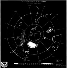
A satellite image of the ozone hole (pink area) over Antarctica taken on September 25, 1995.

The Problem

For four months of every year, Antarctica's McMurdo Research Station lies shrouded in darkness. Then the first rays of light peek out over the horizon. Each day, the sun lingers in the sky, just a little longer and the harsh polar winter slowly gives way to spring.

Spring also brings another type of light to the Antarctic, a light that harms instead of nurtures. In this season of new beginnings, the hole in the ozone layer reforms, allowing lethal ultraviolet radiation to stream through Earth's atmosphere.

The hole lasts for only two months, but its timing could not be worse. Just as sunlight awakens activity in dormant plants and animals, it also delivers a dose of harmful ultraviolet radiation. After eight weeks, the hole leaves Antarctica, only to pass over more populated areas, including New Zealand and Australia. This biologically damaging, high-energy radiation can

cause skin cancer, injure eyes, harm the immune system, and upset the fragile balance of an entire ecosystem.

Although, two decades ago, most scientists would have scoffed at the notion that industrial chemicals could destroy ozone high up in the atmosphere, researchers now know that chlorine creates the hole by devouring ozone molecules. Years of study on the ground, in aircraft, and from satellites has conclusively identified the source of the chlorine: human-made chemicals called chlorofluorocarbons (CFCs) that have been used in spray cans, foam packaging, and refrigeration materials.

All About Ozone

Ozone is a relatively simple molecule, consisting of three oxygen atoms bound together. Yet it has dramatically different effects depending upon its location. Near Earth's surface, where ozone comes into direct contact with life forms, it primarily displays a destructive side. Because it reacts strongly with other molecules, large concentrations of ozone near the ground prove toxic to living things. At higher altitudes, where 90 percent of our planet's ozone resides, it does a remarkable job of absorbing ultraviolet radiation. In the absence of this gaseous shield in the stratosphere, the harmful radiation has a perfect portal through which to strike Earth.

Although a combination of weather conditions and CFC chemistry conspire to create the thinnest ozone levels in the sky above the South Pole, CFCs are mainly released at northern latitudes—mostly from Europe, Russia, Japan, and North America—and play a leading role in lowering ozone concentrations around the globe.

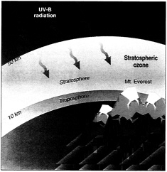
Stratospheric ozone occupies the region of the atmosphere between 10 and 50 kilometers from Earth's surface and provides a shield against damaging ultraviolet radiation.

Worldwide monitoring has shown that stratospheric ozone has declined for at least two decades, with losses of about 10 percent in the winter and spring and 5 percent in the summer and autumn in such diverse locations as Europe, North America, and Australia. Researchers now find depletion over the North Pole as well, and the problem seems to be getting worse each year. According to a United Nations report, the annual dose of harmful ultraviolet radiation striking the northern hemisphere rose by 5 percent during the past decade.

During the past 40 years, the world has seen an alarming increase in the incidence of malignant skin cancer; the rate today is tenfold higher than in the 1950s. Although the entire increase cannot be blamed on ozone loss and increased exposure to ultraviolet radiation, there is evidence of a relationship. Scientists estimate that for each 1 percent decline in ozone levels, humans will suffer as much as a 2 to 3 percent increase in the incidence of certain skin cancers.

Exploring Earth's Atmosphere

Like many lines of scientific inquiry, research leading to the prediction and discovery of global ozone depletion and the damaging effects of CFCs followed a path full of twists and turns. Investigators did not set our to determine whether human activity affects our environment nor did they know much about chemical pollutants. Instead, they began with basic questions about the nature of Earth's atmosphere—its composition, density, and temperature distribution.

The composition of our planet's atmosphere fascinated humans long before chemistry became a formal science. “The storm thundered and lightened, and the air was filled with sulfur,” Homer wrote in the Odyssey, referring to the sharp odor, created during thunderstorms, of what later became known as ozone.

By the late 1800s, atmospheric scientists had isolated carbon monoxide and inferred the existence of a second combustible gas in the air, which they tentatively identified as methane, the simplest hydrocarbon. But in attempting to further analyze the composition of the atmosphere, researchers at the turn of the century faced a major stumbling block: virtually all gases, except for molecular nitrogen and oxygen, exist in such minute concentrations that available equipment could not detect them.

Help, however, was on the way. During the 1880s, scientists had begun perfecting a new, highly precise method of identifying a compound by recording a special kind of chemical fingerprint—the particular pattern of wavelengths of light it emits or absorbs. Scientists call this pattern a spectrum.

In the 1920s, G.M.B. Dobson developed a spectrometer that could measure small concentrations of ozone. By measuring the spectrum of air, the Belgian scientist M.V. Migeotte demonstrated in 1948 that methane is a common constituent of the atmosphere with a concentration of about one part per million by volume. Soon, scientists had the tools to detect other atmospheric gases that occur in concentrations one-tenth to one-hundredth as great as that. By the 1950s, researchers had identified 14 atmospheric chemical constituents.

Despite this progress, researchers were still missing a major piece of the atmospheric puzzle. All of the compounds detected possessed an even number of electrons, a characteristic which typically gives chemical stability. Other less common compounds with an odd number of electrons—known as free radicals—readily undergo chemical reactions and do not survive for long. These compounds play crucial roles in such phenomena as urban smog, the loss of stratospheric ozone, and the global removal of atmospheric impurities.

Scientists had not detected free radicals because they reside in the atmosphere at concentrations well below the part-per-million level that state-of-the-art equipment in 1948 could detect. But unrelated research in an entirely different field, analytical chemistry, soon came to the rescue. Analytical chemists had begun developing a cavalcade of new instruments and methods to measure minute quantities of compounds in the laboratory.

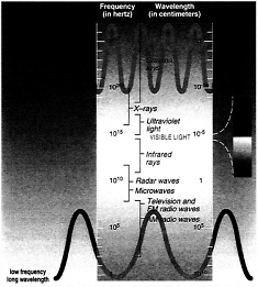
Cancer-causing ultraviolet radiation occupies the region of the spectrum between visible light and even higher frequency radiation such as x-rays and gamma rays.

Such research spurred advances on two fronts: a substantial increase in the precision and accuracy of measurements of atmospheric gases and a striking decrease in the minimum concentration of a compound that must be present to be detected. As a result, the number of atmospheric compounds identified by scientists has increased from 14 in the early 1950s to more than 3,000 today. Detectors today routinely measure compounds at concentrations below one part per trillion, and some can record gases that occur in concentrations one-thousandth as great at that.

The hole lasts for only two months, but its timing could not be worse. Just as sunlight awakens activity in dormant plants and animals, it also delivers a dose of harmful ultraviolet radiation.

Even in some of the most remote locations on Earth, scientists have detected hundreds of compounds. Curiously, some of the substances that occur in the smallest concentrations rank as some of the biggest players in altering the atmosphere. A case in point: the group of chemicals known as CFCs.

Enter the CFCs

CFCs were invented about 65 years ago during a search for a new, nontoxic substance that could serve as a safe refrigerant. One of these new substances, often known by the DuPont trademark Freon, soon replaced ammonia as the standard cooling fluid in home refrigerators. It later became the main coolant in automobile air conditioners.

The 1950s and 1960s saw CFCs used in a variety, of other applications: as a propellant in aerosol sprays, in manufacturing plastics, and as a cleanser for electronic components. All this activity doubled the worldwide use of CFCs every six to seven years. By the early 1970s, industry used about a million tons every year.

Yet as recently as the late 1960s, scientists remained unaware that CFCs could affect the atmosphere. Their ignorance was not from lack of interest, but from lack of tools. Detecting the minuscule concentrations of these compounds in the atmosphere would require a new generation of sensitive detectors.

After developing such a detector, the British scientist James Lovelock, in 1970, became the first to detect CFCs in the air. He reported that one of these compounds, CFC-11, had an atmospheric concentration of about 60 parts per trillion. To put that measurement in perspective, the concentration of methane (natural gas) is 25,000 times greater. Twenty years earlier, merely detecting methane had been considered a major feat.

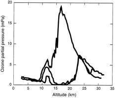
Ozone loss over the South Pole in 1995 (in green) compared with 1993 (in red). The blue line shows values before ozone destruction began.

S OURCE. National Oceanic and Atmospheric Administration.

Lovelock found CFC-11 in every air sample that passed over Ireland from the direction of London. That was not surprising, because most major cities, including London, widely used CFCs. However, Lovelock also detected CFC-11 from air samples

Advances in Atmospheric Science and Policy Decisions Through 1996

This timeline shows the chain of events leading to prediction of the ozone depletion phenomenon, recognition of its consequences, and eventual actions to avert a threatened disaster. It is rich in examples of how basic research often contributes to unanticipated outcomes of immense societal benefit.

Christian Friedrich Schönbein identifies ozone as a component of the lower atmosphere and names it.

W.N. Hartley identifies ozone as the substance that absorbs ultraviolet radiation from the sun at wavelengths below 290 nanometers. He also shows that ozone resides primarily at high altitudes.

1913–1932

C. Fabry and M. Buisson show that the total amount of ozone in a vertical column of the atmosphere can be measured and that it equals (in modern units) 300 Dobson units.

G.M.B. Dobson sets up a regular program of ozone measurements at Oxford with his newly developed spectrophotometer.

Sydney Chapman explains how sunlight striking molecular oxygen in the atmosphere generates ozone.

As part of the International Geophysical Year, four to five research stations in Antarctica begin making regular ozone measurements.

The Nimbus series of satellites begins making ozone measurements.

James Lovelock uses his electron capture detector to measure chlorofluorocarbons(CFCs).

Richard Stolars and Ralph Cicerone disco stratospheric chlorine chain reaction.

directly off the North Atlantic, uncontaminated by recent urban pollution.

This unexpected discovery prompted Lovelock to do further studies. Accordingly, he asked the British government for a modest sum of money to place his apparatus on board a ship traveling from England to Antarctica. His request was rejected; one reviewer commented that even if such a measurement succeeded, he could not imagine a more useless bit of knowledge than finding the atmospheric concentration of CFC-11.

But Lovelock persisted. Using his own money, he put his experiment aboard the research vessel Shackleton in 1971. Two years later the British researcher reported that his shipboard apparatus had detected CFC-11 in every one of the more than 50 air samples collected in the North and South Atlantic. Lovelock correctly concluded that the gas was carried by large-scale wind motions. He also stated that CFCs were not hazardous to the environment, a conclusion soon to be proven wrong.

Ozone Loss: The Chemical Culprits

In 1972, the life of atmospheric scientist F. Sherwood Rowland took a critical turn when he heard a lecture describing Lovelock's work. Like other researchers at the time, Rowland had no inkling that CFCs could harm the environment, but the injection into the atmosphere of large quantities of previously unknown compounds piqued his interest. What would be the ultimate fate of these compounds? Rowland, joined by Mario Molina, a colleague at the University of California, Irvine, decided to find out.

The scientists showed that CFCs remained undisturbed in the lower atmosphere for decades. Invulnerable to visible sunlight, nearly insoluble in water, and resistant to oxidation, CFCs display an impressive durability in the atmosphere's lower depths. But at altitudes above 18 miles, with 99 percent of all air molecules lying beneath them, CFCs show their vulnerability. At this height, the harsh, high-energy ultraviolet radiation from the sun impinges directly on the CFC molecules, breaking them apart into chlorine atoms and residual fragments.

If Rowland and Molina had ended their CFC study with these findings, no one other than atmospheric scientists would ever have heard about it. However, scientific completeness required that the researchers explore not only the fate of the CFCs, but also of the highly reactive atomic and molecular fragments generated by the ultraviolet radiation.

In examining these fragments, Rowland and Molina were aided by prior basic research on chemical

Sherwood Rowland and Mario Molina discover that CFCs can destroy ozone the stratosphere.

The National Academy of Sciences releases its report verifying the Rowland-Molina finding.

The Food and Drug Administration and the Environmental Protection Agency announce a phase-out of CFCs in aerosols.

CFCs used in aerosols are banned in the United States.

A British research group led by Joseph Farman detects a 40 percent ozone loss over Antarctica during spring in the southern hemisphere.

NASA satellite data confirm the existence of the ozone hole over the Antarctic.

The Montreal Protocol is signed, calling for eventual worldwide CFC reduction by 50 percent.

The United States ratifies the Montreal Protocol in a unanimous vote.

Scientists present preliminary findings of a hole in the ozone layer over the Arctic.

Complete ban on industrial production of CFCs goes into effect.

F. Sherwood Rowland, Mario Molina, and Paul Crutzen awarded the Nobel prize for their work in atmospheric chemistry.

kinetics—the study of how quickly molecules react with one another and how such reactions take place. Scientists had demonstrated that a simple laboratory experiment will show how rapidly a particular reaction takes place, even if the reaction involves the interaction of a chlorine atom with methane at an altitude of 18 miles and a temperature of −60 degrees Fahrenheit.

Rowland and Molina did not have to carry out even a single laboratory experiment on the reaction rates of chlorine atoms. They had only to look up the rates already measured by other scientists. Basic research into chemical kinetics had reduced a decade's worth of work to two or three days.

After reviewing the pertinent reactions, the two researchers determined that most of the chlorine atoms combine with ozone, the form of oxygen that protects Earth from ultraviolet radiation. When chlorine and ozone react, they form the free radical chlorine oxide, which in turn becomes part of a chain reaction. As a result of that chain reaction, a single chlorine atom can remove as many as 100,000 molecules of ozone.

Unknown to Rowland and Molina, the same chlorine atom chain reaction had been discovered a few months earlier by Richard Stolarski and Ralph Cicerone. In 1974, Rowland and Molina made a disturbing prediction: If industry continued to release a million tons of CFCs into the atmosphere each year, atmospheric ozone would eventually drop by 7 to 13 percent.

To make matters worse, other scientists had demonstrated that an entirely different group of compounds could further reduce ozone levels. Paul Crutzen first showed in 1970 that nitrogen oxides react catalytically with ozone, playing an important role in the natural ozone balance. Soil-borne microorganisms produce nitrogen oxides as a decay product, and Crutzen's work spotlighted how microbe-rich agricultural fertilizers might lead to reduced ozone levels. His research and that of Harold Johnston also focused attention on the effect of nitrogen oxides spewed by high-altitude aircraft. These emissions may also reduce ozone levels in the stratosphere.

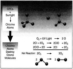
Chlorine atoms induce the decomposition of two ozone molecules into three oxygen molecules in a net chain reaction in which the chlorine atoms are regenerated so that decomposition of ozone continues.

Earlier studies, which had investigated whether exhaust emissions from the supersonic transport and other high-speed aircraft could damage the environment, had already begun to document the effects of ozone loss. Compiled because of the perceived threat from these aircraft, the data were brought to bear on the very real threat from CFCs and nitrogen oxides.

With less ozone in the atmosphere, more ultraviolet radiation reaches Earth. Scientists estimated that increased exposure would lead to a higher incidence of skin cancer, cataracts, and damage to the immune system and to slowed plant growth. Because some CFCs persist in the atmosphere for more than 100 years, these effects would last throughout the twenty-first century.

Concluding that such long-term hazards were unacceptable, Rowland and Molina called for a ban on further release of CFCs. Alerted to this clear and present danger, the United States, Canada, Norway, and Sweden in the late 1970s banned the use of CFCs in aerosol sprays.

The Ozone Hole Emerges

As it turned out, the ozone problem was far worse than Rowland and Molina could have imagined. The first warning signs of a bigger crisis did not appear until the late 1970s, but the studies that uncovered these findings had their roots in research dating back nearly a century.

In the 1880s, W.N. Hartley discovered that a broad band of ultraviolet light reaches Earth almost unimpeded. This band, known as UV-A, has wavelengths just slightly shorter than ordinary visible light. The ozone layer partly absorbs another ultraviolet band, known as UV-B, before it can reach Earth. During the 1920s, G.M.B. Dobson managed to measure the ratio of UV-A to UV-B in incoming sunlight. By doing so, he determined for the first time the total amount of ozone in the atmosphere.

Dobson had hoped his study would lead to a new method of predicting the weather. Instead, he became interested in the seasonal variations in ozone concentrations. An instrument that he developed, the Dobson spectrometer, has become the standard for monitoring ozone from the ground.

When chlorine and ozone react, they form the free radical chlorine oxide, which in turn becomes part of a chain reaction. As a result of that chain reaction, a single chlorine atom can remove as many as 100,000 molecules of ozone.

The rapid development of new scientific tools after World War II—many of them based on wartime instrumentation—led to a flowering of studies in earth science. In 1957–1958, this led to a worldwide scientific effort known as the International Geophysical Year (IGY). IGY sparked an international outpouring of research on the oceans, the atmosphere, and unexplored land areas of the planet.

Monitoring ozone levels in the south polar region, researchers found them to be consistently about 35 percent higher in late spring than in winter. Annual monitoring showed the same seasonal pattern through the late 1970s.

But in 1978 and 1979, the British scientists found something different. In October, the beginning of spring in the southern hemisphere, the researchers detected less ozone than had been detected during the past 20 years. During the next several years, October ozone levels continued to decline.

In 1984, when the British first reported their disturbing findings, October ozone levels were about 35 percent lower than the average for the 1960s. The U.S. satellite Nimbus-7 quickly confirmed the results, and the term Antarctic ozone hole entered popular language.

The Evidence Mounts

By the mid 1980s, scientists had become expert in measuring the concentration of chlorine-containing compounds in the stratosphere. Some monitored the compounds from the ground; others used balloons or aircraft. In 1986 and 1987, these scientists, including Susan Solomon and James Anderson, established that the unprecedented ozone loss over Antarctica involved atomic chlorine and chlorine oxide radicals.

At the same time, measurements in the lower atmosphere established that CFC levels had increased steadily and dramatically since the first recordings taken by Lovelock in 1970. The conclusion was clear: The prime sources of the ozone-devouring chlorine atoms over Antarctica were the CFCs and two other pollutants, the industrial solvents carbon tetrachloride and methylchloroform.

A satellite operated by the National Aeronautics and Space Administration appears to have removed any possible doubt about the role of CFCs. Data collected over the past three years by the Upper Atmosphere Research Satellite revealed these compounds in the stratosphere. Moreover, the satellite has traced the worldwide accumulation of stratospheric fluorine gases, a direct breakdown product of CFCs. The quantitative balance of CFCs and its products eliminates the possibility that chlorine from volcanic eruptions or other natural sources created the ozone hole.

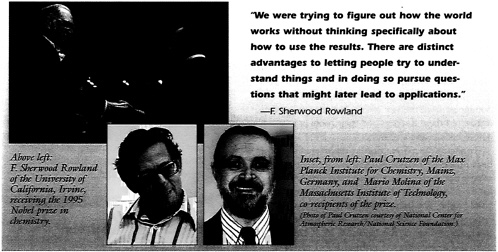
The Outcome: Potential Catastrophe Averted

Painstaking research on ozone and the atmosphere over the past 40 years has led to a global ban on CFC production. Since 1987, more than 150 countries have signed an international agreement, the Montreal Protocol, which called for a phased reduction in the release of CFCs such that the yearly amount added to the atmosphere in 1999 would be half that of 1986. Modifications of that treaty called for a complete ban on CFCs which began in January 1996. Even with this ban in effect, chlorine from CFCs will continue to accumulate in the atmosphere for another decade. It may take until the middle of the next century for ozone levels in the Antarctic to return to 1970s levels.

More globally, ozone depletion is expected to remain a fact of life for several decades to come, but thanks to the research that led to early recognition of the problem and steps that have been taken to address it, the potential consequences are much less severe than they otherwise would have been.

Scientists estimate, for example, that if active research in stratospheric chemistry had not been in place at the time the ozone hole was discovered in 1985 and confirmed in 1986, global ozone depletion, measuring 4 percent today, would be close to 10 percent by the year 2000. Even larger ozone depletion would have been observed over the United States and Eastern Europe, substantially exceeding the current measurements there of about 10 percent loss in winter and spring and 5 percent in summer and autumn. These larger losses have been avoided because basic research in the atmospheric sciences had already advanced to a level where it was able to explain the chemical reactions occurring in the ozone layer. That knowledge allowed other informed political and regulatory decisions to be made

In 1995, the Royal Swedish Academy of Sciences awarded Rowland, Molina, and Crutzen the Nobel prize in chemistry for showing “how sensitive the ozone layer is to the influence of anthropogenic emissions of certain compounds.” In explaining the chemical mechanisms that affect the thickness of the ozone layer, “the three researchers have contributed to our salvation from a global environment problem that could have catastrophic consequences,” the academy noted.

As lawmakers and the public face new challenges in the struggle to protect the environment, they will increasingly rely on basic research to open new vistas and suggest new solutions about these pressing concerns.

Like an infection that grows more and more virulent, the continent-size hole in Earth's ozone layer keeps getting bigger and bigger.

Each year since the late 1970s, much of the protective layer of stratospheric ozone above Antarctica has disappeared during September, creating what is popularly known as the ozone hole. The Antarctic hole now measures about 9 million square miles, nearly the size of North America. Less dramatic, still significant, depletion of ozone levels has been recorded around the globe. With less ozone in the atmosphere, more ultraviolet radiation strikes Earth, causing more skin cancer, eye damage, and possible harm to crops.

READ FREE ONLINE

Welcome to OpenBook!

You're looking at OpenBook, NAP.edu's online reading room since 1999. Based on feedback from you, our users, we've made some improvements that make it easier than ever to read thousands of publications on our website.

Do you want to take a quick tour of the OpenBook's features?

Show this book's table of contents , where you can jump to any chapter by name.

...or use these buttons to go back to the previous chapter or skip to the next one.

Jump up to the previous page or down to the next one. Also, you can type in a page number and press Enter to go directly to that page in the book.

Switch between the Original Pages , where you can read the report as it appeared in print, and Text Pages for the web version, where you can highlight and search the text.

To search the entire text of this book, type in your search term here and press Enter .

Share a link to this book page on your preferred social network or via email.

View our suggested citation for this chapter.

Ready to take your reading offline? Click here to buy this book in print or download it as a free PDF, if available.

Get Email Updates

Do you enjoy reading reports from the Academies online for free ? Sign up for email notifications and we'll let you know about new publications in your areas of interest when they're released.

Share full article

Supported by

Richard Benedick, Negotiator of Landmark Ozone Treaty, Dies at 88

He played a key role in securing the Montreal Protocol, an international environmental pact to protect the ozone layer by reducing the use of certain chemicals.

Richard Benedick in a black-and-white photo wearing a suit, glasses and a patterned tie while sitting next to a globe.

By Trip Gabriel

A May 1985 report in the journal Nature was alarming. High above Antarctica, a massive hole had opened in the ozone shield that protects life on earth from the sun’s ultraviolet rays.

The finding confirmed what scientists had warned of since the 1970s : Atmospheric ozone was being broken down by the wide use of chlorofluorocarbons, chemicals known as CFCs, which were found in aerosol sprays, refrigeration and air-conditioning.

Just over two years later, dozens of nations meeting in Montreal signed an agreement to significantly reduce CFCs, which the Environmental Protection Agency estimated would prevent 27 million deaths from skin cancers.

“This is perhaps the most historically significant international environmental agreement,” Richard E. Benedick, the chief United States negotiator, said at the time .

Ever since, the Montreal Protocol, as the pact is known, has stood as a milestone of collective action in the face of a planetary environmental threat, as well as a rebuke of the lack of international resolve to tackle the more dire and complex threat of climate change.

Mr. Benedick, who was a career diplomat in the State Department when the Montreal Protocol was signed in 1987, and who patiently wore down opposition from foreign nations while withstanding powerful internal critics in the Reagan administration, died on March 16 in Falls Church, Va. He was 88.

His daughter, Julianna Benedick, confirmed the death. She said that he had suffered from advanced dementia and that he had been living in a memory care home since 2018.

It is no small paradox that a global treaty to address atmospheric pollution was negotiated during the presidency of Ronald Reagan, who was elected as a champion of business and a sworn enemy of government regulations.

But support for addressing the threat of CFCs to human health was possible because environmental issues were less bitterly partisan than they would later become, and because U.S. industry — chiefly DuPont, the largest maker of the chemicals — preferred an international treaty to the possibility of more draconian cuts by Congress.

Still, as Mr. Benedick wrote in a 1991 book about the road to a deal, “Ozone Diplomacy: New Directions in Safeguarding the Planet,” success was never assured during the nine months in which the treaty was hammered out. “Most observers in and out of government,” he wrote, “believed at that time that an agreement on international regulation of CFCs would be impossible to reach.”

Mr. Benedick, whom colleagues described as energetic and dogged, was instrumental to the success. “He was a tenacious guy; he was like a terrier with a bone,” John D. Negroponte, then an assistant secretary of state who was Mr. Benedick’s superior and ally, said in an interview. “The atmosphere in this town — it was an uphill fight; I don’t think it would have happened without him.”

In the Reagan administration, leaders of the State Department and the Environmental Protection Administration favored regulating CFCs. But in the middle of the international talks, strong opposition emerged from Donald P. Hodel, the interior secretary, and William R. Graham Jr., the White House science adviser.

Mr. Hodel said Americans worrying about skin cancer from ozone loss should not expect more government regulation, but should try “personal protection,” namely hats, sunglasses and sunscreen.

His comments, once leaked to the press, were widely mocked, inspiring editorial cartoons of fish and animals — which are also at risk from ultraviolet rays — in sunglasses. Environmentalists greeted Mr. Hodel at a news conference with their faces smeared white with sunscreen.

Other opposition came from foreign countries, chiefly Japan, the Soviet Union and the European bloc, which argued that the scientific link between CFCs and ozone depletion was not proved.

The State Department sent key scientists from the U.S. government’s science agencies to Moscow, Tokyo and Brussels to educate their counterparts.

“I think it helped get the message across,” Mr. Negroponte said. “Dick was the brains behind that.”

In the end, President Reagan came down on the side of Mr. Benedick and the State Department, overruling the anti-regulatory faction in his administration. Among the reasons suggested for the decision was that Mr. Reagan had recently had a cancerous growth removed.

The Montreal Protocol, which required cutting the use of CFCs by half, was signed by 24 countries in September 1987. It was ratified unanimously the next year by the U.S. Senate. In 1990, the protocol was toughened to eventually phase out CFCs entirely. Today, nearly every country in the world has banned them.

Concentrations of long-lived ozone-depleting chemicals in the stratosphere have gradually declined, with the ozone hole above Antarctica expected to heal by the 2060s, according to the National Oceanic and Atmospheric Administration.

Richard Elliott Benedick was born on May 10, 1935, in the Bronx. His father, Lester L. Benedick, was in the insurance business. His mother, Rose (Katz) Benedick, died while giving birth, and as a result, Mr. Benedick’s daughter said, “He never liked celebrating his birthday.”

Lester Benedick remarried to Jean (Shamsky) Benedick.

Richard, raised in the Bronx, earned a bachelor’s degree in economics from Columbia University, an M.A. in economics from Yale and a Ph.D. from the Harvard Business School. His dissertation was titled “Industrial Finance in Iran.”

In 1957 he married Hildegard Schulz, whom he met at the International House at Yale. She accompanied Mr. Benedick, then a foreign service officer specializing in economic development in the State Department, to postings in Iran, Pakistan, France and Germany. The couple divorced in 1982.

Mr. Benedick’s second marriage, to Helen Freeman, also ended in divorce. Later he had a long-term companion, Irene Federwisch. In addition to his daughter, from his first marriage, he is survived by a son, Andreas Benedick, also from that marriage; a granddaughter; and two great-grandchildren.

At the time of the Montreal Protocol, Mr. Benedick was deputy assistant secretary of state for environment, health and natural resources and coordinator of population affairs.

“Richard was energetic, even passionate,” said William K. Reilly, who was president of the World Wildlife Fund, where Mr. Benedick was a fellow after negotiating the Montreal Protocol. “It was a career highlight for him and for the United States, a masterful diplomatic achievement.”

When he returned to the State Department under President George H.W. Bush, Mr. Benedick attempted to apply ozone diplomacy to the issue of global warming, which scientists had begun to warn was the most perilous environmental threat. A government scientist, James Hansen, told the Senate and the press in 1988 that the evidence that global warming had begun could be detected “with 99 percent confidence.” His statement became front-page news.

Mr. Reilly, who led the E.P.A. under Mr. Bush, said the politics of the administration did not favor action. Secretary of State James A. Baker III “chose to recuse himself from climate,” Mr. Reilly said. Mr. Bush’s chief of staff, John H. Sununu, vetoed a proposal from the E.P.A . to have the president propose a global treaty on carbon emissions. When Mr. Hansen reappeared before the Senate in 1989, the White House censored his testimony to inject doubts that human activity caused climate change.

Mr. Benedick was not a scientist, but he was a great admirer of nature and the outdoors.

“He absolutely loved taking our family to the national parks,” Ms. Benedick, his daughter, said. “He planned five cross-country trips when we were children in the ’70s and ’80s. We’d fly to California and visited pretty much every national park driving east. He’d have us get up at the crack of dawn to watch the sunrise over Yosemite or Bryce or Zion or Monument Valley.”

Trip Gabriel is a national correspondent. He covered the past two presidential campaigns and has served as the Mid-Atlantic bureau chief and a national education reporter. He formerly edited the Styles sections. He joined The Times in 1994. More about Trip Gabriel

Scientific Assessment of Ozone Depletion: 2022

Twenty questions and answers about the ozone layer, twenty questions and answers about the ozone layer: 2022 update, recommended citation, twenty questions and answers about the ozone layer citation:.

Ross J. Salawitch (Lead Author), Laura A. McBride, Chelsea R. Thompson, Eric L. Fleming, Richard L. McKenzie, Karen H. Rosenlof, Sarah J. Doherty, David W. Fahey, Twenty Questions and Answers About the Ozone Layer: 2022 Update, Scientific Assessment of Ozone Depletion: 2022 , 75 pp., World Meteorological Organization, Geneva, Switzerland, 2023.

The Twenty Questions and Answers About the Ozone Layer: 2022 Update is a component of the Scientific Assessment of Ozone Depletion: 2022 report. The report is prepared quadrennially by the Scientific Assessment Panel (SAP) of the Montreal Protocol on Substances that Deplete the Ozone Layer . The 2022 edition of the Twenty Questions document is the fifth update of the original edition that appeared in the 2002 Assessment Report. The motivation behind this scientific publication is to tell the story of ozone depletion, ozone-depleting substances and the success of the Montreal Protocol. The questions and answers format divides the narrative into topics that can be read and studied individually by the intended audience of specialists and non-specialists. The topics range from the most basic (e.g., What is ozone?) to more recent developments (e.g., the Kigali Amendment to the Montreal Protocol). Each question begins with a short answer followed by a longer, more comprehensive answer. Figures enhance the narrative by illustrating key concepts and results. This document is principally based on scientific results presented in the 2022 and earlier Assessment Reports and has been extensively reviewed by scientists and non-specialists to ensure quality and readability.

We hope that you find this Twenty Questions and Answers edition of value in communicating the scientific basis of ozone depletion and the success of the Montreal Protocol in protecting the ozone layer and climate.

David W. Fahey, Paul A. Newman, John A. Pyle, and Bonfils Safari Co-Chairs of the Scientific Assessment Panel

Introduction

Ozone is present only in small amounts in the atmosphere. Nevertheless, ozone is vital to human well-being as well as agricultural and ecosystem sustainability. Most of Earth's ozone resides in the stratosphere, the layer of the atmosphere that is more than 10 kilometers (6 miles) above the surface. About 90% of atmospheric ozone is contained in the stratospheric "ozone layer", which shields Earth's surface from harmful ultraviolet radiation emitted by the Sun.

In the mid-1970s scientists discovered that some human-produced chemicals could lead to depletion of the stratospheric ozone layer. The resulting increase in ultraviolet radiation at Earth's surface would increase incidents of skin cancer and eye cataracts, suppress the immune systems of humans, and also adversely affect agriculture as well as terrestrial and oceanic ecosystems.

Following the discovery of this environmental issue, researchers sought a better understanding of this threat to the ozone layer. Monitoring stations showed that the abundances of gases that are ozone-depleting substances (ODSs), such as chlorofluorocarbons (CFCs), were steadily increasing in the atmosphere. These trends were linked to growing production and use of CFCs and other ODSs for spray can propellants, refrigeration and air conditioning, foam blowing, industrial cleaning, and other applications. Measurements in the laboratory and in the atmosphere characterized the chemical reactions that were involved in ozone destruction. Computer models of the atmosphere employing this information were used to simulate how much ozone depletion was already occurring and to predict how much more might occur in the future.

By the mid-1980s observations of the ozone layer showed that depletion was indeed occurring. The most severe ozone loss, unexpected at the time of discovery, was found to be recurring each springtime over Antarctica. The loss in this region is commonly called the "ozone hole" because the ozone depletion is so large and localized. A thinning of the ozone layer also has been observed over other regions of the globe, such as the Arctic and northern and southern midlatitudes.

The work of many scientists throughout the world has built a broad and solid scientific understanding of the ozone-depletion process. With this foundation, we know that ozone depletion has been occurring and we understand why. Most importantly, we know that if the most potent ODSs were to continue to be emitted and increase in the atmosphere, the result would be ever greater depletion of the ozone layer.

In 1985, the world's governments adopted the Vienna Convention for the Protection of the Ozone Layer in response to the prospect of increasing ozone depletion. The Vienna Convention provided a framework through which nations agreed to take appropriate measures to protect human health and the environment from activities that harm the ozone layer, including cooperation on systematic observations, research and exchange of information. In 1987, this framework led to the Montreal Protocol on Substances that Deplete the Ozone Layer (the Montreal Protocol), an international treaty designed to control the production and consumption of CFCs and other ODSs. As a result of the broad compliance with the Montreal Protocol and subsequent amendments and adjustments as well as industry's development and deployment of "ozone-friendly" substitutes to replace CFCs, the total global accumulation of ODSs in the atmosphere has begun to decrease.

The replacement of CFCs has occurred in two phases: first via the use of hydrochlorofluorocarbons (HCFCs) that cause considerably less damage to the ozone layer compared to CFCs, and second by the introduction of hydrofluorocarbons (HFCs) that do not deplete ozone. In response, global ozone depletion has stabilized, and initial signs of recovery of the ozone layer are being observed. With continued compliance, substantial recovery of the ozone layer is expected by the middle of the 21st century. The day the Montreal Protocol was agreed upon, 16 September, is now celebrated as the International Day for the Preservation of the Ozone Layer. The Montreal Protocol has also decreased the human drivers of global warming, because many CFCs and HFCs are potent greenhouse gases (GHGs).

The amendment and adjustment process is a vitally important aspect of the Montreal Protocol, allowing the protocol to evolve and address emerging issues as our scientific understanding matures. The Protocol was amended or adjusted between 1990 and 2007 at meetings held in London, Copenhagen, Vienna, Beijing, and Montreal (see Q14). The most recent amendment was formulated at the Meeting of the Parties of the Montreal Protocol held in Kigali, Rwanda during October 2016. The Kigali Amendment phases down future global production and consumption of some HFCs to protect future climate, an important new milestone for the Montreal Protocol (see Q19). The Kigali Amendment was motivated by projections of substantial increases in the global use of HFCs in the coming decades. The control of HFCs under this amendment marks the first time the Montreal Protocol has adopted controls solely for the protection of climate.

The protection of the ozone layer and climate under the Montreal Protocol is a story of notable achievements: discovery, understanding, decisions, actions, and verification. It is a success story written by many: scientists, technologists, economists, legal experts, and policymakers, in which continuous dialogue has been a key ingredient. A timeline of milestones related to the science of stratospheric ozone depletion, international scientific assessments, and the Montreal Protocol is illustrated in Figure Q0-1 .

Stratospheric ozone depletion and policy milestones

To help communicate the broad understanding of the Montreal Protocol, ODSs, and ozone depletion, as well as the relationship of these topics to GHGs and global warming, this component of the Scientfic Assessment of Ozone Depletion: 2022 report describes the state of this science with 20 illustrated questions and answers. The questions and answers address the nature of atmospheric ozone, the chemicals that cause ozone depletion, how global and polar ozone depletion occur, the extent of ozone depletion, the success of the Montreal Protocol, the possible future of the ozone layer, and the protection against climate change now provided by the Kigali Amendment. Computer model projections show that GHGs such as carbon dioxide (CO 2 ), methane (CH 4 ), and nitrous oxide (N 2 O) will have a growing influence on global ozone in the coming decades, and in some cases may exceed the influence of ODSs on ozone by the middle of this century, given the expected future decline in the atmospheric abundance of ODSs.

For each question, a brief answer is first given in highlighted text; an expanded answer then follows. The answers are based on the information presented in the 2022 and earlier Assessment reports as well as other international scientific assessments. These reports and the answers provided here were prepared and reviewed by a large number of international scientists who are experts in different research fields related to the science of stratospheric ozone and climate 2 .

1 Here and throughout, the term ozone-depleting substances (ODSs) refers to gases containing either chlorine or bromine that are released to the atmosphere as a result of human activity and are controlled under Annexes A, B, C, or E of the Montreal Protocol.

2 See Appendix for Acknowledgments .

Ozone in our atmosphere

Q1 what is ozone, how is it formed, and where is it in the atmosphere.

Ozone is a gas that is naturally present in our atmosphere. Each ozone molecule contains three atoms of oxygen and is denoted chemically as O 3 . Ozone is found primarily in two regions of the atmosphere. About 10% of Earth's ozone is in the troposphere, which extends from the surface to about 10-15 kilometers (6-9 miles) altitude. About 90% of Earth's ozone resides in the stratosphere, the region of the atmosphere between the top of the troposphere and about 50 kilometers (31 miles) altitude. The part of the stratosphere with the highest amount of ozone is commonly referred to as the "ozone layer". Throughout the atmosphere, ozone is formed in multistep chemical processes that are initiated by sunlight. In the stratosphere, the process begins with an oxygen molecule (O 2 ) being broken apart by ultraviolet radiation from the Sun. In the troposphere, ozone is formed by a different set of chemical reactions that involve naturally occurring gases as well as those from sources of air pollution.

Ozone is a gas that is naturally present in our atmosphere. Ozone has the chemical formula O 3 because an ozone molecule contains three oxygen atoms (see Figure Q1-1 ). Ozone was discovered in laboratory experiments in the mid-1800s. Ozone's presence in the atmosphere was later discovered using chemical and optical measurement methods. The word ozone is derived from the Greek word óζειν (ozein) , meaning "to smell." Ozone has a pungent odor that allows it to be detected even at very low amounts. Ozone reacts rapidly with many chemical compounds and is explosive in concentrated amounts. Electrical discharges are generally used to produce ozone for industrial processes such as air and water purification and bleaching of textiles and food products.

Ozone location. Most ozone (about 90%) is found in the stratosphere, which begins about 10-15 kilometers (km) above Earth's surface and extends up to about 50 km altitude. The stratospheric region with the highest concentration of ozone, between about 15 and 35 km altitude, is commonly known as the "ozone layer" (see Figure Q1-2 ). The stratospheric ozone layer extends over the entire globe, with some variation in its altitude and thickness. Most of the remaining ozone (about 10%) is found in the troposphere, which is the lowest region of the atmosphere, between Earth's surface and the stratosphere. Tropospheric air is the "air we breathe" and, as such, excess ozone in the troposphere has harmful consequence (see Q2 ).

Ozone abundance. Ozone molecules constitute a small fraction of the gas molecules in the atmosphere. Most air molecules are either oxygen (O 2 ) or nitrogen (N 2 ). In the stratosphere, near the peak concentration of the ozone layer, there are typically a few thousand ozone molecules for every billion air molecules (1 billion = 1,000 million). In the troposphere near Earth's surface, ozone is even less abundant, with a typical range of 20 to 100 ozone molecules for each billion air molecules. The highest ozone values near the surface occur in air that is polluted by human activities. Throughout this document the word “abundance” refers to the concentration or amount of an atmospheric gas or some other physical quantity.

As an illustration of the low relative abundance of ozone in our atmosphere, one can imagine bringing all the ozone molecules in the troposphere and stratosphere down to Earth's surface and forming a layer of pure ozone that extends over the entire globe. The resulting layer would have an average thickness of about three millimeters (0.12 inches), which scientists would report as 300 Dobson Units (see Q3 ). Nonetheless, this extremely small fraction of the atmosphere plays a vital role in protecting life on Earth (see Q2 ).

Stratospheric ozone. Stratospheric ozone is formed naturally by chemical reactions involving solar ultraviolet radiation (sunlight) and oxygen molecules, which make up about 21% of the atmosphere. In the first step, solar ultraviolet radiation breaks apart one oxygen molecule (O 2 ) to produce two oxygen atoms (2 O) (see Figure Q1-3 ). In the second step, each of these highly reactive oxygen atoms combines with an oxygen molecule to produce an ozone molecule (O 3 ). These reactions occur continually whenever solar ultraviolet radiation is present in the stratosphere. As a result, the largest ozone production occurs in the tropical stratosphere.

The production of stratospheric ozone is balanced by its destruction in chemical reactions. Ozone reacts continually with sunlight and a wide variety of natural and human-produced chemicals in the stratosphere. In each reaction, an ozone molecule is lost and other chemical compounds are produced. Important reactive gases that destroy ozone are hydrogen and nitrogen oxides and those containing chlorine and bromine (see Q7 ). Some stratospheric ozone is regularly transported down into the troposphere and can occasionally influence ozone amounts at Earth's surface.

Tropospheric ozone. Near Earth's surface, ozone is produced by chemical reactions involving gases emitted into the atmosphere from both natural sources and human activities. Ozone production in the troposphere primarily occurs by reactions of hydrocarbon and nitrogen oxide gases, and all require sunlight for completion. Fossil fuel combustion and deforestation are the primary sources of pollutant gases that lead to production of tropospheric ozone. As in the stratosphere, ozone in the troposphere is destroyed by naturally occurring chemical reactions and by reactions involving human-produced chemicals. Tropospheric ozone can also be destroyed when ozone reacts with a variety of surfaces, such as those of soils and plants.

Balance of chemical processes. Ozone abundances in the stratosphere and troposphere are determined by the balance between chemical processes that produce and destroy ozone. The balance is determined by the amounts of reactive gases and how the rate or effectiveness of the various reactions varies with sunlight intensity, location in the atmosphere, temperature, and other factors. As atmospheric conditions change to favor ozone-producing reactions in a certain location, ozone abundances increase. Similarly, if conditions change to favor other reactions that destroy ozone, abundances decrease. The balance of production and loss reactions, combined with atmospheric air motions that transport and mix air with different ozone abundances, determines the global distribution of ozone on timescales of days to many months (see also Q3 ). Global stratospheric ozone decreased from the 1970s to the late 1990s (see Q12 and Q13 ) because the amounts of reactive gases containing chlorine and bromine in the stratosphere increased due to human activities (see Q6 and Q15 ).

Q2 Why do we care about atmospheric ozone?

Ozone in the stratosphere absorbs a large part of the Sun's biologically harmful ultraviolet radiation. Stratospheric ozone is considered "good" ozone because of this beneficial role. In contrast, ozone formed at Earth's surface in excess of natural amounts is considered “bad” ozone because this gas is harmful to humans, plants, and animals.

Ozone in the stratosphere (Good ozone) . Stratospheric ozone is considered good for humans and other life forms because ozone absorbs ultraviolet (UV) radiation from the Sun (see Figure Q2-1 ). The Sun emits UV radiation that scientists categorize into three wavelength ranges: UV-C (100 to 280 nanometer (nm) wavelengths); UV-B (280 to 315 nm), and UV-A (315 to 400 nm). The energy of solar UV radiation, which cannot be seen by the human eye, is higher at shorter wavelengths. Exposure to high energy UV-C radiation is particularly dangerous to all life forms. Fortunately, UV-C radiation is entirely absorbed within the ozone layer. Most UV-B radiation emitted by the Sun is absorbed by the ozone layer; the rest reaches Earth's surface. In humans, increased exposure to UV-B radiation raises the risks of skin cancer and cataracts, and suppresses the immune system. Exposure to UV-B radiation before adulthood and cumulative exposure are both important health risk factors. Excessive UV-B exposure also can damage terrestrial plant life, including agricultural crops, single-celled organisms, and aquatic ecosystems. Low energy UV radiation, UV-A, which is not absorbed significantly by the ozone layer, causes premature aging of the skin.

Protecting stratospheric ozone. In the mid-1970s, it was discovered that gases containing chlorine and bromine atoms released by human activities could cause stratospheric ozone depletion (see Q5 and Q6 ). These gases, referred to as halogen source gases, and also as ozone-depleting substances (ODSs), chemically release their chlorine and bromine atoms after they reach the stratosphere. Ozone depletion increases surface UV-B radiation above naturally occurring amounts. International efforts have been successful in protecting the ozone layer through controls on the production and consumption of ODSs (see Q14 and Q15 ).

UV Protection by the Stratospheric Ozone Layer

Ozone in the troposphere (Bad ozone) . Ozone near Earth's surface in excess of natural amounts is considered bad ozone (see Figure Q1-2 ). Surface ozone in excess of natural levels is formed by reactions involving air pollutants emitted from human activities, such as nitrogen oxides (NOx), carbon monoxide (CO), and various hydrocarbons (gases containing hydrogen, carbon, and often oxygen). Exposure to ozone at concentrations above natural levels is harmful to humans, plants, and other living systems because ozone reacts strongly to destroy or alter molecules that constitute biological tissue. Enhanced surface ozone caused by air pollution reduces crop yields and forest growth. In humans, exposure to high levels of ozone can reduce lung capacity; cause chest pains, throat irritation, and coughing; and worsen pre-existing health conditions related to the heart and lungs. In addition, increases in tropospheric ozone lead to a warming of Earth's surface because ozone is a greenhouse gas (GHG) (see Q17 ). The negative effects of excess tropospheric ozone contrast sharply with the protection from harmful UV radiation afforded by preserving the natural abundance of stratospheric ozone.

Reducing tropospheric ozone. Limiting the emission of certain common pollutants reduces the production of excess ozone near Earth's surface, where ozone can affect humans, plants, and animals. Major sources of pollutants include large cities, where fossil fuel consumption for transportation, heating, and industrial activities is concentrated, power plants that rely on coal, oil, or natural gas, as well as deforestation, wildfires, and the burning of savannah for agriculture. Many programs around the globe have been successful in reducing or limiting the emission of pollutants that cause production of excess ozone near Earth's surface.

Natural ozone. In the absence of human activities, ozone would still be present near Earth's surface and throughout the troposphere and stratosphere because ozone is a natural component of the clean atmosphere. Natural emissions from the biosphere, mainly from trees, participate in chemical reactions that produce ozone. Atmospheric ozone plays important ecological roles beyond absorbing UV radiation. For example, ozone initiates the chemical removal of many pollutants as well as some GHGs, such as methane (CH 4 ). In addition, the absorption by ozone of solar UV radiation as well as visible and infrared radiation is a natural source of heat in the stratosphere, causing temperatures to increase with altitude. Stratospheric temperatures affect the balance of ozone production and destruction processes (see Q1 ) and air motions that redistribute ozone throughout the stratosphere (see Q3 ).

Q3 How is total ozone distributed over the globe?

The distribution of total ozone over Earth varies with geographic location and on daily and seasonal time-scales. These variations are caused by large-scale movements of stratospheric and tropospheric air and the chemical production and destruction of ozone. Total ozone is generally lowest at the equator and highest in midlatitude and polar regions.

Total ozone. The total column of ozone at any location on the globe is defined as the sum of all the ozone in the atmosphere directly above that location. Most ozone resides in the stratospheric ozone layer and a small percentage (about 5 to 10%) is distributed throughout the troposphere (see Q1 ). Total column ozone values are usually reported in Dobson units denoted as "DU." Typical values vary between 200 and 500 DU over the globe, with a global average abundance of about 300 DU (see Figure Q3-1 ). The ozone molecules required for total ozone to be 300 DU would form a layer of pure ozone gas at Earth's surface having a thickness of only 3 millimeters (0.12 inches) (see Q1 ), which is about the height of a stack of 2 common coins, if these molecules could be isolated and compressed. It is remarkable that a layer of pure ozone only 3 millimeters thick protects life on Earth's surface from most of the harmful UV radiation emitted by the Sun (see Q2 ).

Global distribution. Total ozone varies strongly with latitude over the globe, with the largest values occurring at middle and high latitudes during most of the year (see Figure Q3-1 ). This distribution is the result of the large-scale circulation of air in the stratosphere that slowly transports ozone-rich air from high altitudes in the tropics, where ozone production from solar ultraviolet radiation is largest, toward the poles. Ozone accumulates at middle and high latitudes, increasing the vertical extent of the ozone layer and, at the same time, total ozone. The total column of ozone is generally smallest in the tropics for all seasons. An exception since the mid-1980s is the region of low values of ozone over Antarctica during spring in the Southern Hemisphere, a phenomenon known as the Antarctic ozone hole (dark blue, Figure Q3-1 ; also see Q10 and Q11 ).

Seasonal distribution. Total ozone also varies with season, as shown in Figure Q3-1 using two-week averages of ozone taken from satellite observations acquired in 2021. March and September plots represent the early spring and autumn seasons in the Northern and Southern Hemispheres, respectively. June and December plots similarly represent the early summer and winter seasons. During spring, total ozone exhibits maximums at latitudes poleward of about 45° N in the Northern Hemisphere and between 45° and 60° S in the Southern Hemisphere. These spring maximums are a result of increased transport of ozone from its source region in the tropics toward high latitudes during late autumn and winter. This poleward ozone transport is much weaker during the summer and early autumn periods and is weaker overall in the Southern Hemisphere.

This natural seasonal cycle can be observed clearly in the Northern Hemisphere as shown in Figure Q3-1 , with increasing values in Arctic total ozone during winter, a clear maximum in spring, and decreasing values from summer to autumn. In the Antarctic, however, a pronounced minimum in total ozone is observed during spring. The minimum is known as the "ozone hole", which is caused by the widespread chemical depletion of ozone in spring by pollutants known as ozone-depleting substances (see Q5 and Q10 ). In the late 1970s, before the ozone hole appeared each year, much higher ozone values than those currently observed were found in the Antarctic spring (see Q10 ). Currently, the lowest values of total ozone across the globe and all seasons are found during early spring in the Antarctic, as shown in Figure Q3-1 . After spring, these low values disappear from total ozone maps as polar air mixes with lower-latitude air containing much higher amounts of ozone.

In the tropics, the change in total ozone through the progression of the seasons is much smaller than at higher latitudes. This feature is present because seasonal changes in both sunlight and ozone transport are much smaller in the tropics compared to higher latitudes.

The abundance of ozone is larger at midlatitudes in the Northern Hemisphere (NH) than the Southern Hemisphere (SH), for all four seasons in the respective hemispheres. The thinner ozone layer at SH midlatitudes compared to NH midlatitudes is due to several factors: differences in the large-scale circulation of the two hemispheres that preceded the development of the ozone hole as well as larger abundances of tropospheric ozone in the NH compared to the SH that is caused by more pollution in the more heavily populated NH. Dilution of ozone-depleted air from the Antarctic ozone hole region starting in the 1980s further increases the hemispheric difference in total ozone. This hemispheric total ozone difference results in higher levels of UV light reaching the surface in the SH compared to the NH (see Q16 ).

Natural variations. Total ozone varies strongly with latitude and longitude, as seen within the seasonal plots in Figure Q3-1 . These patterns come about for two reasons. First, atmospheric winds transport air between regions of the stratosphere that have high ozone values and those that have low ozone values. Tropospheric weather systems can temporarily alter the vertical extent of the ozone layer in a region, and thereby change total ozone. The regular nature of these air motions, in some cases associated with geographical features (oceans and mountains), in turn causes recurring patterns in the distribution of total ozone. Second, ozone variations occur as a result of changes in the balance of chemical production and loss processes. This balance is very sensitive to the amount of solar UV radiation (see Q2 ) reaching the various parts of the atmosphere.

There is a good understanding of how chemistry and air motions work together to cause the observed large-scale features in total ozone, such as those seen in Figure Q3-1 . Ozone changes are routinely monitored by a large group of scientists using satellite, airborne, and ground-based instruments. The continued analyses of these observations provide an important long-term basis to quantify the contribution of human activities to ozone depletion.

Global Satellite Maps of Total Ozone in 2021

Q4 How is ozone measured in the atmosphere?

The amount of ozone in the atmosphere is measured by instruments on the ground and carried aloft on balloons, aircraft, and satellites. Some instruments measure ozone remotely over long distances by using ozone's unique optical absorption or emission properties. Other instruments measure ozone locally by continuously drawing air samples into a small detection chamber.

The abundance of ozone in the atmosphere is measured by a variety of techniques (see Figure Q4-1 ). The techniques make use of ozone's unique optical and chemical properties. There are two principal categories of measurement techniques: local and remote. Ozone measurements by these techniques have been essential in monitoring changes in the ozone layer and in developing our understanding of the processes that control ozone abundances.

Local measurements. Local measurements of the atmospheric abundance of ozone are those that require air to be drawn directly into an instrument. Once inside an instrument's detection chamber, the amount of ozone is determined by measuring the absorption of ultraviolet (UV) radiation or by the electrical current or light produced in a chemical reaction involving ozone. The latter approach is used in "ozonesondes", which are lightweight, ozone-measuring modules suitable for launching on small balloons. The balloons ascend up to altitudes of about 32 to 35 kilometers (km), high enough to measure ozone in the stratospheric ozone layer. Ozonesondes are launched regularly at many locations around the world. Local ozone-measuring instruments using optical or chemical detection schemes are also used on research aircraft to measure the distribution of ozone in the troposphere and lower stratosphere (up to altitudes of about 20 km). High-altitude research aircraft can reach the ozone layer at most locations over the globe and can reach furthest into the layer at high latitudes. Ozone measurements are also being made routinely on some commercial aircraft flights. Local measurements of the abundance of ozone at the surface are obtained at many thousands of sites over the globe, which provide hourly data critical for assessing and improving air quality throughout the world.

Remote measurements. Remote measurements of total ozone amounts and the altitude distributions of ozone are obtained by detecting ozone at large distances from the instrument. Most remote measurements of ozone rely on its unique absorption of UV radiation. Sources of UV radiation that can be used are sunlight (and reflected sunlight from the moon), lasers, and starlight. For example, satellite instruments use the absorption of solar UV radiation by the atmosphere or the absorption of sunlight scattered from the surface of Earth to measure ozone over nearly the entire globe on a daily basis. Lidar instruments, which measure backscattered laser light, are routinely deployed at ground sites and on research aircraft to detect ozone over a distance of many kilometers along the laser light path. A network of ground-based instruments measures ozone by detecting small changes in the amount of the Sun's UV radiation that reaches Earth's surface. Other instruments measure ozone using either its absorption of infrared, visible, or ultraviolet radiation or its emission of microwave or infrared radiation at different altitudes in the atmosphere, thereby obtaining information on the vertical distribution of ozone. Emission measurements have the advantage of providing remote ozone measurements at night, which is particularly valuable for sampling polar regions during winter, when there is continuous darkness.

The ozone depletion process

Q5 how do emissions of halogen source gases lead to stratospheric ozone depletion.

The initial step in the depletion of stratospheric ozone by human activities is the emission, at Earth's surface, of gases that contain chlorine and bromine and have long atmospheric lifetimes. Most of these gases accumulate in the lower atmosphere because they are relatively unreactive and do not dissolve readily in rain or snow. Natural air motions eventually transport these accumulated gases to the stratosphere, where they are converted to more reactive gases. Some of these gases then participate in reactions that destroy ozone. Finally, when stratospheric large-scale circulation patterns return this air to the lower atmosphere, these reactive chlorine and bromine gases are removed from Earth's atmosphere by rain and snow.

The principal steps in stratospheric ozone depletion caused by human activities are shown in Figure Q5-1 .

Emission, accumulation, and transport. The process begins with the emission , at Earth's surface, of long-lived source gases containing the halogens chlorine and bromine ( Q6 ). The halogen source gases, often referred to as ozone-depleting substances (ODSs), include manufactured chemicals released to the atmosphere when used in a variety of applications, such as refrigeration, air conditioning, and foam blowing. Chlorofluorocarbons (CFCs) are an important example of chlorine-containing source gases. Emitted source gases accumulate in the lower atmosphere (troposphere) and are slowly transported to the stratosphere by natural air motions. The accumulation occurs because most source gases are highly unreactive in the lower atmosphere. Furthermore, only a small amount of halogen source gases dissolve in ocean waters. The low reactivity of these manufactured halogenated gases within the lower atmosphere is one property that made them well suited for specialized applications such as refrigeration.

Some halogen gases are emitted in substantial quantities from natural sources (see Q6 ). These emissions also accumulate in the troposphere, are transported to the stratosphere, and participate in ozone destruction reactions. These naturally emitted gases are part of the natural balance of ozone production and destruction that predates the large release of manufactured halogenated gases and the associated observed ozone depletion.

Conversion, reaction, and removal. Halogen source gases do not react directly with ozone. Once in the stratosphere, halogen source gases are chemically converted to reactive and reservoir halogen gases by the absorption of ultraviolet radiation from the Sun (see Q7 ). The rate of conversion is related to the atmospheric lifetime of a gas (see Q6 ). Gases with longer lifetimes have slower conversion rates and survive longer in the atmosphere after emission. Lifetimes of the principal ODSs vary from about 1 to 100 years (see Table Q6-1 ). Emitted gas molecules with atmospheric lifetimes greater than a few decades circulate between the troposphere and stratosphere multiple times, on average, before conversion occurs.

The reactive gases formed from halogen source gases react chemically to destroy ozone in the stratosphere (see Q8 ). The average depletion of total ozone attributed to reactive gases is smallest in the tropics and largest at high latitudes (see Q12 ). In polar regions, reactions that occur on the surface of polar stratospheric clouds, which exist only at low temperatures, greatly increase the abundance of the most important reactive chlorine gas, chlorine monoxide (ClO) (see Q9 ). his process results in substantial ozone destruction in polar regions in late winter/early spring (see Q10 and Q11 ).

Air in the stratosphere is generally isolated from the troposphere. A small portion of stratospheric air returns to the troposphere every day, bringing along reactive and reservoir halogen gases. On average, it takes several years for air throughout the global stratosphere to return to the troposphere. Reactive halogen gases that are transported back to the troposphere are removed from the atmosphere by rain and other precipitation or deposited by wind onto Earth's land or ocean surfaces. These removal processes bring to an end the destruction of ozone by chlorine and bromine atoms that were first released to the atmosphere as components of halogen source gas molecules.

Tropospheric conversion. Halogen source gases with short lifetimes (less than 1 year) undergo significant chemical conversion in the troposphere, producing reactive and reservoir halogen gases. Source gas molecules that are not converted are transported to the stratosphere. Only small portions of reactive and reservoir halogen gases produced in the troposphere are transported to the stratosphere, because most are removed by precipitation. Important examples of halogen gases that undergo some tropospheric removal, prior to transport to the stratosphere, are the hydrochlorofluorocarbons (HCFCs), methyl bromide (CH 3 Br), methyl chloride (CH 3 Cl), and gases containing iodine (see Q6 ).

Principal Steps in the Depletion of Stratospheric Ozone

Q6 What emissions from human activities lead to ozone depletion?

Certain industrial processes and consumer products result in the emission of ozone-depleting substances (ODSs) to the atmosphere. Principal ODSs are manufactured halogen source gases that are now controlled worldwide by the Montreal Protocol. These gases bring chlorine and bromine atoms to the stratosphere, where they destroy ozone in chemical reactions. Important examples are the chlorofluorocarbons (CFCs), once used in almost all refrigeration and air conditioning systems, and the halons, which were used as fire extinguishing agents. Current ODS abundances in the atmosphere are known directly from air sample measurements.

Halogen source gases versus ozone-depleting substances (ODSs). Halogen source gases that are emitted by human activities and controlled by the Montreal Protocol are generally referred to as ODSs. The Montreal Protocol controls the global production and consumption of ODSs (see Q14 ). Halogen source gases such as methyl chloride (CH 3 Cl) that have predominantly natural sources are not classified as ODSs. The contributions of various ODSs and natural halogen source gases to the total amount of chlorine and bromine entering the stratosphere are shown in Figure Q6-1 . Total chlorine and total bromine entering the stratosphere peaked in 1993 and 1999, respectively. The difference in the timing of these peaks is a result of various phaseout schedules specified by the Montreal Protocol and its amendments and adjustments, different atmospheric lifetimes of halogen source gases, and the time delays between production and emission of the numerous source gases. Also shown are the contributions to total chlorine and bromine in 2020, highlighting the reductions of 11% and 15%, respectively, achieved by the controls of the Montreal Protocol.

Ozone-depleting substances (ODSs). The principal ODSs are manufactured for specific industrial uses or consumer products, most of which result in the eventual emission of these gases to the atmosphere. Total ODS emissions increased substantially from the middle to the late 20th century, reached a peak in the late 1980s, and are now in decline (see Figure Q0-1 ). Because of their long atmospheric lifetimes, a large fraction of the emitted ODSs reach the stratosphere, where they are converted to reactive and reservoir gases containing chlorine and bromine that lead to ozone depletion.

ODSs containing only carbon, chlorine, and fluorine are called chlorofluorocarbons , usually abbreviated as CFCs. The principal CFCs are CFC-11 (CCl 3 F), CFC-12 (CCl 2 F 2 ), and CFC-113 (CCl 2 FCClF 2 ). CFCs, along with carbon tetrachloride (CCl 4 ) and methyl chloroform (CH 3 CCl 3 ), historically have been the most important chlorine-containing halogen source gases emitted by human activities. These and other chlorine-containing ODSs have been used in many applications, including refrigeration, air conditioning, foam blowing, spray can propellants, and cleaning of metals and electronic components. As a result of the Montreal Protocol controls, the abundances of these chlorine source gases have decreased since 1993 (see Figure Q6-1 ). The concentrations of CFC-11 and CFC-12 peaked in 1994 and 2002, respectively, and have since decreased (see Figure Q15-1 ). The abundances of CFC-11 and CFC-12 in 2020 were 16% and 2.8% lower than their values in 1993, respectively.

The class of compounds known as hydrochlorofluorocarbons (HCFCs) contain hydrogen, in addition to chlorine, fluorine, and carbon. HCFC-22 (CHF 2 Cl), developed in the 1930s, has been used as a refrigerant, primarily in residential air conditioners, since the 1940s. As detailed below, HCFCs are less harmful to the ozone layer compared to CFCs. In the 1990s, the use of HCFC-22 expanded and other HCFCs were developed as substitutes for CFCs. Consequently, the chlorine content of HCFCs entering the stratosphere increased by 185% between 1993 and 2020 (see Figure Q6-1 ). With restrictions on production starting in 1996, and globally in place since 2013, the atmospheric abundances of HCFCs are expected to peak between 2023 and 2030 (see Figures Q0-1 and Q15-1 ). Classes of compounds known as hydrofluorocarbons (HFCs) and hydrofluoroolefins (HFOs) constitute the replacement for many applications of HCFCs.

Another category of ODSs contains bromine. The most important of these gases are the halons and methyl bromide (CH 3 Br). Halons are a group of industrial compounds that contain at least one bromine and one carbon atom; halons may or may not contain a chlorine atom. Halons were originally developed to extinguish fires and were widely used to protect large computer installations, military hardware, and commercial aircraft engines. Consequently, halons are often released directly into the atmosphere upon use or testing of these fire suppression systems. The most abundant halons emitted by human activities are halon-1211 (CBrClF 2 ) and halon-1301 (CBrF 3 ). Methyl bromide is used primarily as a fumigant for pest control in agriculture and disinfection of export shipping goods, and also has significant natural sources.

As a result of the controls of the Montreal Protocol, the contribution to the atmospheric abundance of methyl bromide from human activities decreased by 71% between 1999 and 2020 (see Figure Q6-1 ). The concentration of halon-1211 peaked in 2005 and has been decreasing ever since, reaching an abundance in 2020 that was 22% below that measured in 1999. The abundance of halon-1301, on the other hand, increased by 19% since 1999 and is expected to slowly decline into the next decade because of continued small releases and a long atmospheric lifetime (see Figure Q15-1 ). In 2020, the bromine content of other halons (mainly halon-1202 and halon-2402) was 25% below the amount present in 1999.

Natural sources of chlorine and bromine. There are a few halogen source gases present in the stratosphere that have large natural sources. These include methyl chloride (CH 3 Cl) and methyl bromide (CH 3 Br), both of which are emitted by oceanic and terrestrial ecosystems. In addition, very short-lived source gases (defined as compounds with atmospheric lifetimes typically less than 0.5 year) containing bromine such as bromoform (CHBr3) and dibromomethane (CH 2 Br 2 ) are also released to the atmosphere, primarily from biological activity in the oceans. Only a fraction of the emissions of very short-lived source gases reaches the stratosphere because these gases are efficiently removed in the lower atmosphere. Volcanoes provide an episodic source of reactive halogen gases that sometimes reach the stratosphere in appreciable quantities.

Other natural sources of halogens include reactive chlorine and bromine produced by evaporation of ocean spray. However, these reactive chemicals play no role in stratospheric ozone depletion because they readily dissolve in water and are removed in the troposphere.

In 2020, natural sources contributed about 17% of total stratospheric chlorine and about 56% of total stratospheric bromine (see Figure Q6-1 ). The amount of chlorine and bromine entering the stratosphere from natural sources is known to be fairly constant over time and, therefore, cannot be the cause of the ozone depletion observed since the 1980s.

Halogen Source Gases Entering the Stratosphere

Other human activities that are sources of chlorine and bromine gases. Other chlorine- and bromine-containing gases are released to the atmosphere from human activities. Common examples are the use of chlorine-containing solvents and industrial chemicals, and the use of chlorine gases in paper production and disinfection of potable and industrial water supplies (including swimming pools). Most of these gases are very short-lived and only a small fraction of their emissions reaches the stratosphere. The contribution of very short-lived chlorinated gases from natural sources and human activities to total stratospheric chlorine was 63% larger in 2020 than in 1993, and now contributes about 4% (130 ppt) of the total chlorine entering the stratosphere (see Figure Q6-1 ). The Montreal Protocol does not control the production and consumption of very short-lived chlorine source gases, although the atmospheric abundances of some (notably dichloromethane, CH 2 Cl 2 ) have increased substantially in recent years. Solid rocket engines, such as those used to propel payloads into orbit, release reactive chlorine gases directly into the troposphere and stratosphere. The quantities of chlorine emitted globally by rockets is currently small in comparison with halogen emissions from other human activities.

Lifetimes and emissions. Estimates of global emissions in 2020 for a selected set of halogen source gases are given in Table Q6-1 . These emissions occur from continued production of HCFCs and HFCs as well as the release of gases from banks. Emission from banks refers to the atmospheric release of halocarbons from existing equipment, chemical stockpiles, foams, and other products. In 2020 the global emission of the refrigerant HCFC-22 constituted the largest annual release, by mass, of a halocarbon from human activities. Release in 2020 of HFC-134a (CH 2 FCF 3 ), another refrigerant, was second largest. The emission of methyl chloride (CH 3 Cl) is primarily from natural sources such as the ocean biosphere, terrestrial plants, salt marshes and fungi. The human source of methyl chloride is small relative to the total natural source (see Q15 ).

After emission, halogen source gases are either removed from the atmosphere or undergo chemical conversion in the troposphere, stratosphere, or mesosphere. The time to remove or convert about 63% of a gas is often called its atmospheric lifetime. Lifetimes vary from less than 1 year to 100 years for the principal chlorine- and bromine-containing gases (see Table Q6-1 ). The long-lived gases are converted to other gases primarily in the stratosphere and essentially all of their original halogen content becomes available to participate in the destruction of stratospheric ozone. Conversely, gases with short lifetimes such as methyl bromide, methyl chloride, and some HCFCs are converted to other gases in the troposphere, which are then removed from the atmosphere by rain and snow. Therefore, only a fraction of their halogen content contributes to ozone depletion in the stratosphere. Methyl chloride, despite its large source, constituted only about 17% (540 ppt) of the halogen source gases entering the stratosphere in 2020 (see Figure Q6-1 ).

The amount of an emitted gas that is present in the atmosphere represents a balance between its emission and removal rates. A wide range of current emission rates and atmospheric lifetimes are derived for the various source gases (see Table Q6-1 ). The atmospheric abundances of most of the principal CFCs and halons have decreased since 1990 in response to smaller emission rates, while those of the important substitute gases, the HCFCs, continue to slowly increase under the provisions of the Montreal Protocol (see Q15 ). In the past few years, the rate of the increase of the atmospheric abundance of HCFCs has declined. In the coming decades, the emissions and atmospheric abundances of all controlled ODSs are expected to decrease under these provisions.

Ozone Depletion Potential (ODP). The effectiveness of halogen source gases at destroying stratospheric ozone is given by the ODP (see Table Q6-1 and Q17 ). A gas with a larger ODP destroys more stratospheric ozone than a gas with a smaller ODP. The calculation of ODP requires the use of computer models that simulate atmospheric ozone and is found relative to CFC-11, which has an ODP defined to be 1. The ODP of a gas is based upon a comparison of the amount of ozone depletion caused by the continuous emission to the atmosphere of a certain mass of that gas, relative to the amount of ozone depletion following emission of the same mass of CFC-11. Halogen source gases controlled by the Montreal Protocol have a wide range of ODPs. Halon-1211 and halon-1301 have ODPs significantly larger than that of CFC-11 and most other chlorinated gases because bromine is much more effective (about 60 times) on a per-atom basis than chlorine in chemical reactions that destroy ozone. The gases with smaller values of ODP generally have shorter atmospheric lifetimes or contain fewer chlorine and bromine atoms compared to gases with larger ODPs.

HFCs & other fluorine-containing gases. Many of the source gases in Figure Q6-1 also contain fluorine, another halogen, in addition to chlorine or bromine. After the source gases undergo conversion in the stratosphere (see Q5 ), the fluorine content of these gases is left in chemical forms that do not cause ozone depletion. As a consequence, halogen source gases that contain fluorine and no other halogens are not classified as ODSs. An important example of these are the HFCs, which are included in Table Q6-1 because they are common ODS substitute gases. HFCs do not contain chlorine or bromine and, consequently, all HFCs have an ODP of zero.

Many HFCs are strong greenhouse gases, as quantified by a metric termed the Global Warming Potential (GWP) (see Q17 ). The Kigali Amendment to the Montreal Protocol now controls the production and consumption of HFCs (see Q19 ), especially those HFCs with high GWPs. As a result, industry has transitioned in part to production and use of a subset of HFCs with very low GWPs known as hydrofluoroolefins (HFOs), which are also composed of hydrogen, fluorine, and carbon atoms. Here, the "O" stands for olefin, a term used by chemists to refer to the double carbon bond of these compounds that results in small tropospheric lifetimes and GWPs for HFOs. One such HFO, HFO-1234yf (CF 3 CFCH 2 ), has a GWP of less than 1 due to its 12 day lifetime.

Iodine containing gases. Iodine is a component of several gases that are naturally emitted from the oceans and from some human activities. Research on the importance of iodine for stratospheric ozone is being conducted, in part, because trifluoroiodomethane (CF 3 I) is a possible replacement for halons in fire extinguishers and also because CF 3 I has been proposed as an ingredient of low-GWP refrigerant blends. Although iodine can participate in ozone destruction reactions, iodine-containing source gases all have very short lifetimes, with most of the removal occurring in the lower atmosphere within a few days. Since the last assessment, there has been an upward revision to the upper limit on the amount of iodine reaching the stratosphere, which is now estimated to be about 1 ppt. The importance for stratospheric ozone of very short-lived iodine containing source gases, including a possible enhancement of polar ozone depletion, remains an active area of investigation.

Other non-halogen gases. Other non-halogen gases that influence stratospheric ozone abundances have also increased in the stratosphere as a result of emissions from human activities (see Q20 ). Important examples are methane (CH 4 ), which reacts in the stratosphere to form water vapor and reactive hydrogen, and nitrous oxide (N 2 O), which reacts in the stratosphere to form nitrogen oxides. These reactive products participate in the destruction of stratospheric ozone. Increased levels of atmospheric carbon dioxide (CO 2 ) alter stratospheric temperature and winds, which also affect the abundance of stratospheric ozone. Should future atmospheric abundances of CO 2 , CH 4 and N 2 O increase significantly relative to present-day values, these increases will affect future levels of stratospheric ozone through combined effects on temperature, winds, and chemistry (see Figure Q20-2 ). Efforts are underway to reduce the emissions of these gases under the Paris Agreement of the United Nations Framework Convention on Climate Change because they cause surface warming (see Q18 and Q19 ). Although past emissions of ODSs still dominate global ozone depletion today, future emissions of N 2 O from human activities are expected to become relatively more important for ozone depletion as the atmospheric abundances of ODSs decline (see Q20 ).

Table Q6-1. Atmospheric lifetimes, global emissions, Ozone Depletion Potentials, and Global Warming Potentials of some halogen source gases and HFC substitute gases.

a Includes both human activities (production and banks) and natural sources. Emissions are in units of kilotonnes per year (1 kilotonne = 1000 metric tons = 1 gigagram = 10 9 grams). These emission estimates are based on analysis of atmospheric observations. The range of values for each emission estimate reflects the uncertainty in estimating emissions from atmospheric observations.

b 100-year GWP. ODPs and GWPs are discussed in Q17 . Values are calculated for emissions of an equal mass of each gas. ODPs given here reflect current scientific values and in some cases differ from those used in the Montreal Protocol.

Q7 What are the reactive halogen gases that destroy stratospheric ozone?

Chlorine and bromine containing halogen source gases that enter the stratosphere arise from both human activities and natural processes ( Q6 ). When exposed to ultraviolet radiation from the Sun, these halogen source gases are converted to other gases that also contain chlorine and bromine. Some of the gases act as chemical reservoirs, which can then be converted into ClO and BrO, the two most important reactive gases that participate in catalytic reactions that destroy ozone.

Halogen-containing gases present in the stratosphere can be divided into two groups: halogen source gases as well as reactive and reservoir halogen gases (see Figure Q7-1 ). The source gases, which include ozone-depleting substances (ODSs), are emitted at Earth's surface by natural processes and by human activities (see Q6 ) and are chemically inert in the lower atmosphere. Once in the stratosphere, the halogen source gases chemically convert at different rates to form the reactive and reservoir halogen gases. The conversion occurs in the stratosphere instead of the troposphere because solar ultraviolet (UV) radiation (a component of sunlight) is needed for the breakup of these compounds, and solar UV radiation is more intense in the stratosphere than the troposphere (see Q2 ).Reactive gases containing the halogens chlorine and bromine participate in a series of chemical reactions that remove stratospheric ozone (see Q8 ).

Reactive and reservoir halogen gases. The chemical conversion of halogen source gases, which involves solar ultraviolet radiation and other chemical reactions, produces a number of reactive and reservoir halogen gases. These reactive and reservoir gases contain all of the chlorine and bromine atoms originally present in the source gases. The chlorine content of all of the reactive and reservoir gases is termed available chlorine , while the bromine content of similar gases is termed available bromine .

The most important reactive and reservoir chlorine and bromine containing gases that form in the stratosphere are shown in Figure Q7-1 . Throughout the stratosphere, the most abundant are typically hydrogen chloride (HCl) and chlorine nitrate (ClONO 2 ). These two gases are considered reservoir gases because, while they do not react directly with ozone, they can be converted to the most reactive forms that do chemically destroy ozone. The halogens most reactive with ozone are chlorine monoxide (ClO) and bromine monoxide (BrO) molecules, as well as chlorine and bromine (Cl and Br) atoms. A large fraction of available bromine is generally in the form of BrO, whereas usually only a small fraction of available chlorine is in the form of ClO. The unusually cold conditions that occur in the polar regions during winter cause the reservoir gases HCl and ClONO 2 to undergo nearly complete conversion to ClO and related reactive gases. This conversion occurs through chemical reactions that take place on the surface or within polar stratospheric cloud (PSC) particles (see Q9 ).

Chlorine at midlatitudes. Reactive and reservoir chlorine gases have been observed extensively in the stratosphere using both local and remote measurement techniques, including observations from satellite instruments. The measurements from space displayed in Figure Q7-2 are representative of how the amounts of chlorine-containing gases change between the surface and the upper stratosphere at middle to high latitudes. Total chlorine (see red line in Figure Q7-2 ) is the sum of chlorine contained in halogen source gases (e.g., CFC-11, CFC-12) and in the reservoir and reactive gases (e.g., HCl, ClONO2, and ClO). Total chlorine is constant to within about 10% from the surface to above 50 km (31 miles) altitude. In the troposphere, total chlorine is contained almost entirely in the source gases described in Figure Q6-1 . At higher altitudes, the source gases become a smaller fraction of total chlorine as they are converted to the reactive and reservoir chlorine gases. At the highest altitudes, total chlorine is all in the form of reactive and reservoir chlorine gases.

In the altitude range of the ozone layer at midlatitudes, as shown in Figure Q7-2 , the reservoir gases HCl and ClONO 2 account for most of the available chlorine. The abundance of ClO, the most important reactive gas in ozone depletion, is a small fraction of total chlorine. The abundance of ClO peaks in the upper stratosphere about 40 km (24.9 miles) above the surface. In this region of the atmosphere the abundance of ozone reached a minimum in the late 1990s, at about the time the abundance of ClO in the upper stratosphere maximized. In the lower and middle stratosphere (altitudes below about 30 km, or 18.6 miles above the surface), the low abundance of ClO tends to limit the amount of ozone destruction that occurs outside of polar regions.

Chlorine in polar regions. Chlorine gases in polar regions undergo large changes between autumn and late winter. Meteorological and chemical conditions in both polar regions are now routinely observed from space in all seasons. Maps of autumn and late winter conditions at an altitude of 18 km (11.2 miles), near the center of the ozone layer (see Figure Q11-3) over the Antarctic are contrasted in Figure Q7-3 These observations document dramatic differences in chemistry and temperature for these two seasons.

Ozone values are high over the entire Antarctic continent during autumn in the Southern Hemisphere. Temperatures are mid-range, HCl and nitric acid (HNO 3 ) are high, and ClO is very low. High HCl indicates that substantial conversion of halogen source gases to this reservoir gas has occurred in the stratosphere. In the 1980s and early 1990s, the abundances of the reservoir gases HCl and ClONO 2 increased substantially in the stratosphere following increased emissions of halogen source gases. HNO 3 is an abundant, primarily naturally-occurring stratospheric compound that plays a major role in stratospheric ozone chemistry by both moderating ozone destruction and condensing to form polar stratospheric clouds (PSCs), thereby enabling conversion of chlorine reservoirs gases to ozone-destroying forms (see Q9 ). The low abundance of ClO indicates that little conversion of the reservoir to reactive gases occurs in autumn, thereby limiting chemical ozone destruction.

By late winter (September), a remarkable change in the composition of the Antarctic stratosphere has taken place. Low amounts of ozone reflect substantial depletion at 18 km altitude over an area larger than the Antarctic continent. Antarctic ozone holes arise from similar chemical destruction throughout much of the altitude range of the ozone layer (see altitude profile in Figure Q11-3 ). The meteorological and chemical conditions in late winter, characterized by very low temperatures, very low HCl and HNO 3 , and very high ClO, are distinctly different from those found in autumn. Low stratospheric temperatures occur during winter, when solar heating is reduced. Low HCl and high ClO reflect the conversion of the halogen reservoir compounds, HCl and ClONO 2 , to the most important reactive form of chlorine, ClO. This conversion occurs selectively in winter on PSCs, which form at very low temperatures (see Q9 ). Low HNO 3 is indicative of its condensation to form these PSCs, some of which subsequently fall to lower altitudes through gravitational settling. High abundances of ClO generally cause ozone depletion to continue in the Antarctic region until mid- October (spring), when the lowest ozone values usually are observed (see Q10 ). As temperatures rise at the end of the winter, PSC formation is halted, ClO is converted back into the reservoir species HCl and ClONO 2 (see Q9 ), and ozone destruction is curtailed.

Similar changes in meteorological and chemical conditions are also observed between autumn and late winter for some years in the Arctic, leading to substantial ozone loss. In spring of 2020, Arctic ozone reached exceptionally low values. A very stable, cold, and long-lived stratospheric Arctic vortex enabled halogen-catalyzed chemical ozone loss that exceeded the previous record-breaking loss observed in spring 2011 (see Q11). Substantial chemical loss of Arctic ozone will continue to occur in cold winters/springs, as long as the concentrations of ODSs are well above natural levels.

Bromine observations. Fewer measurements are available for reactive and reservoir bromine gases in the lower stratosphere than for chlorine gases. This difference arises in part because of the lower abundance of bromine, which makes quantification of its atmospheric abundance more challenging. The most widely observed bromine gas is BrO, which can be observed from space. Estimates of the concentration of available bromine in the stratosphere are higher than expected from the decomposition of halons and methyl bromide, the most important bromine source gases that are produced by human activities. This difference was the first direct evidence that very short-lived (VSL) bromine-containing source gases reach the stratosphere. Subsequently, direct observations of VSL source gases have confirmed their importance. In 2020, slightly more than one-quarter of the total stratospheric bromine is supplied by these naturally occurring, VSL source gases (see Q6 ).

Chemical Conditions Observed in the Ozone Layer Over Antarctica

Q8 What are the chlorine and bromine reactions that destroy stratospheric ozone?

Reactive gases containing chlorine and bromine destroy stratospheric ozone in “catalytic” cycles made up of two or more separate reactions. As a result, a single chlorine or bromine atom can destroy many thousands of ozone molecules before it leaves the stratosphere. In this way, a small amount of reactive chlorine or bromine has a large impact on the ozone layer. A special situation develops in polar regions in the late winter/early spring season, where large enhancements in the abundance of the most important reactive gas, chlorine monoxide, lead to severe ozone depletion.

Stratospheric ozone is destroyed by reactions involving reactive halogen gases, which are produced in the chemical conversion of halogen source gases (see Figure Q7-1 ). The most reactive of these gases are chlorine monoxide (ClO), bromine monoxide (BrO), and chlorine and bromine atoms (Cl and Br). These gases participate in three principal reaction cycles that destroy ozone.

Cycle 1. Ozone destruction Cycle 1 is illustrated in Figure Q8-1 . The cycle is made up of two basic reactions: Cl + O 3 and ClO + O. The net result of Cycle 1 is to convert one ozone molecule and one oxygen atom into two oxygen molecules. In each cycle, chlorine acts as a catalyst because ClO and Cl react and are reformed. In this way, one Cl atom participates in many cycles, destroying many ozone molecules. For typical stratospheric conditions at middle or low latitudes, a single chlorine atom can destroy thousands of ozone molecules before it happens to react with another gas, breaking the catalytic cycle. During the total time of its stay in the stratosphere, a chlorine atom can thus destroy many thousands of ozone molecules.

Polar Cycles 2 and 3. The abundance of ClO is greatly increased in polar regions during late winter and early spring, relative to other seasons, as a result of reactions on the surfaces of polar stratospheric clouds (see Q7 and Q9 ). Cycles 2 and 3 (see Figure Q8-2 ) become the dominant reaction mechanisms for polar ozone loss because of the high abundances of ClO and the relatively low abundance of atomic oxygen (which limits the rate of ozone loss by Cycle 1). Cycle 2 begins with the self-reaction of ClO. Cycle 3, which begins with the reaction of ClO with BrO, has two reaction pathways that produce either Cl and Br or BrCl. The net result of both cycles is to destroy two ozone molecules and create three oxygen molecules. Cycles 2 and 3 account for most of the ozone loss observed in the stratosphere over the Arctic and Antarctic regions in the late winter/early spring season (see Q10 and Q11 ). At high ClO abundances, the rate of polar ozone destruction can reach 2 to 3% per day.

Ozone Destruction Cycles in Polar Regions

Sunlight requirement. Sunlight is required to complete and maintain these reaction cycles. Cycle 1 requires ultraviolet (UV) radiation (a component of sunlight) that is strong enough to break apart molecular oxygen into atomic oxygen. Cycle 1 is most important in the stratosphere at altitudes above about 30 km (18.6 miles), where solar UV-C radiation (100 to 280 nanometer (nm) wavelengths) is most intense (see Figure Q2-1 ).

Cycles 2 and 3 also require sunlight. In the continuous darkness of winter in the polar stratosphere, reaction Cycles 2 and 3 cannot occur. Sunlight is needed to break apart (ClO) 2 and BrCl, resulting in abundances of ClO and BrO large enough to drive rapid loss of ozone by Cycles 2 and 3. These cycles are most active when sunlight returns to the polar regions in late winter/early spring. Therefore, the greatest destruction of ozone occurs in the partially to fully sunlit periods after midwinter in the polar stratosphere.

Sunlight in the UV-A (315 to 400 nm wavelengths) and visible (400 to 700 nm wavelengths) parts of the spectrum needed in Cycles 2 and 3 is not sufficient to form ozone because this process requires more energetic solar UV-C solar radiation (see Q1 and Q2 ). In the late winter/early spring, only UV-A and visible solar radiation is present in the polar stratosphere, due to low Sun angles. As a result, the rate of ozone destruction by Cycles 2 and 3 in the sunlit polar stratosphere during springtime greatly exceeds the rate of ozone production.

Other reactions. . Global abundances of ozone are controlled by many other reactions (see Q1 ). Reactive hydrogen and reactive nitrogen gases, for example, are involved in catalytic ozone-destruction cycles, similar to those described above, that also take place in the stratosphere. Reactive hydrogen is supplied by the stratospheric decomposition of water (H 2 O) and methane (CH 4 ). Methane emissions result from both natural sources and a wide variety of human activities. The abundance of stratospheric H 2 O is controlled by the temperature of the upper tropical troposphere as well as the decomposition of stratospheric CH 4 . Reactive nitrogen is supplied by the stratospheric decomposition of nitrous oxide (N 2 O), also emitted by natural sources and human activities. The importance of reactive hydrogen and nitrogen gases in ozone depletion relative to reactive halogen gases is expected to increase in the future because the atmospheric abundances of the reactive halogen gases are decreasing as a result of the Montreal Protocol, while abundances of CH 4 and N 2 O are projected to increase due to various human activities (see Q20 ).

Q9 Why has an "ozone hole" appeared over Antarctica when ozone-depleting substances are present throughout the stratosphere?

Ozone-depleting substances are present throughout the stratospheric ozone layer because they are transported great distances by atmospheric air motions. The severe depletion of the Antarctic ozone layer known as the "ozone hole" occurs because of particular meteorological and chemical conditions that exist there and nowhere else on the globe. The very low winter temperatures in the Antarctic stratosphere cause polar stratospheric clouds (PSCs) to form. Specific chemical reactions that occur on PSCs, combined with the isolation of polar stratospheric air inside the polar vortex, allow chlorine and bromine reactions to produce the ozone hole over Antarctica in springtime.

The severe depletion of stratospheric ozone in late winter and early spring in the Antarctic is known as the "ozone hole" (see Q10 ). The ozone hole appears over Antarctica because meteorological and chemical conditions unique to this region increase the effectiveness of ozone destruction by reactive halogen gases (see Q7 and Q8 ). The formation of the Antarctic ozone hole requires the combination of temperatures low enough to form polar stratospheric clouds (PSCs), isolation of polar vortex air from air in other stratospheric regions, sunlight, and sufficient amounts of available chlorine (see Q8 ).

Minimum Air Temperatures in the Polar Stratosphere

Distribution of halogen gases. Halogen source gases that are emitted at Earth's surface and have lifetimes longer than about 1 year (see Table Q6-1 ) are present in comparable amounts throughout the stratosphere in both hemispheres, even though most of the emissions occur in the Northern Hemisphere. The stratospheric abundances are comparable in both hemispheres because most long-lived source gases have no significant natural removal processes in the lower atmosphere, and because winds and convection redistribute and mix air efficiently throughout the troposphere on the timescale of weeks to months. Halogen source gases enter the stratosphere primarily from the tropical upper troposphere. Stratospheric air motions then transport these gases upward and toward the pole in both hemispheres.

Low polar temperatures. The severe ozone destruction that leads to the ozone hole requires low temperatures to be present over a range of stratospheric altitudes, over large geographical regions, and for an extended period of time. Low temperatures are important because they allow liquid and solid PSC particles to form. Chemical reactions within and on the surfaces of these PSC particles initiate a remarkable increase in the most important reactive chlorine gas, chlorine monoxide (ClO) (see below as well as Q7 and Q8 ). Air is usually too warm to enable the formation of clouds in the stratosphere. Only the polar regions during winter have temperatures low enough for stratospheric clouds to form, because air cools due to lack of sunlight. In the Antarctic winter, minimum daily temperatures are generally much lower and less variable than those in the Arctic winter (see Figure Q9-1 ). Antarctic temperatures also remain below PSC formation temperatures for much longer periods during winter. These and other meteorological differences occur because of variations between the hemispheres in the distributions of land, ocean, and mountains at middle and high latitudes. As a consequence, winter temperatures are low enough for PSCs to form somewhere in the Antarctic for nearly the entire winter (about 5 months), and only for limited periods (about 1 to 4 months) in the Arctic for most winters.

Isolated conditions. Stratospheric air in the polar regions is relatively isolated for long periods in the winter months. This isolation results from strong winds that encircle the poles during winter, forming a polar vortex , which prevents substantial transport and mixing of air into or out of the polar stratosphere. This circulation strengthens in winter as stratospheric temperatures decrease. The polar vortex circulation tends to be stronger in the Southern Hemisphere (SH) than in the Northern Hemisphere (NH), because northern latitudes have more mountainous regions and adjacent areas of ocean and land with contrasting temperatures than is present at southern latitudes. This situation leads to more meteorological disturbances in the circulation of the NH, which increase the mixing in of air from lower latitudes toward the pole, warming the Arctic stratosphere. Since winter temperatures are therefore lower in the SH than in the NH polar stratosphere, the isolation of air in the polar vortex is much more effective in the Antarctic than in the Arctic. Once temperatures drop low enough, PSCs form within the polar vortex and induce chemical changes such as an increase in the abundance of ClO (see Q8 ). These changes persist for many weeks to months due to the isolation of stratospheric air in the Antarctic.

Polar stratospheric clouds (PSCs). Chemical reactions within and on the surfaces of liquid and solid PSC particles can substantially increase the relative abundances of reactive chlorine gases. These reactions convert the reservoir forms of chlorine gases, hydrogen chloride (HCl) and chlorine nitrate (ClONO 2 ) to the most important reactive form, ClO (see Figure Q7-3 ). The abundance of ClO increases from a small fraction of available chlorine to comprise more than half of all available chlorine (see Q7 ). With increased ClO, the catalytic cycles involving ClO and BrO become active in the chemical destruction of ozone whenever sunlight is available (see Q8 ).

Different types of liquid and solid PSC particles form when stratospheric temperatures fall below about -78°C (-108°F) in polar regions (see Figure Q9-1 ). As a result, PSCs are often found over large areas of the winter polar regions and over extensive altitude ranges in both hemispheres, with substantially larger regions and for longer time periods in the Antarctic than in the Arctic. The most common type of PSC forms from nitric acid (HNO 3 ) and water condensing on pre-existing liquid sulfuric acid (H 2 SO 4 )-containing particles. Some of these particles freeze to form solid particles. At even lower temperatures (-85°C or -121°F), water condenses to form ice particles. PSC particles grow large enough and are numerous enough that cloud-like features can be observed from the ground under certain conditions, particularly when the Sun is near the horizon (see Figure Q9-2 ). PSCs are often found near mountain ranges in polar regions because the motion of air over the mountains can cause localized cooling in the stratosphere, which increases condensation of water and HNO 3 .

When average temperatures begin increasing in late winter, PSCs form less frequently, which slows down the conversion of chlorine from reservoir to reactive forms throughout the polar region. Without continued production, the abundance of ClO decreases as other chemical reactions re-form the reservoir gases, ClONO 2 and HCl. When temperatures rise above PSC formation thresholds, usually sometime between late January and early March in the Arctic and by mid-October in the Antarctic (see Figure Q9-1 ), the most intense period of ozone depletion ends.

Arctic Polar Stratospheric Clouds (PSCs)

Nitric acid and water removal. Once formed, the largest PSC particles fall to lower altitudes because of gravity. The largest particles can descend several kilometers in the stratosphere within a few days during the low-temperature winter/spring period. Because PSCs often contain a significant fraction of available HNO 3 , their descent removes HNO 3 from regions of the ozone layer. This process is called denitrification of the stratosphere. Because HNO 3 is a source for nitrogen oxides (NOx) in the stratosphere, denitrification removes the NOx available for converting the highly reactive chlorine gas ClO back into the reservoir gas ClONO 2 . As a result, ClO remains chemically active for a longer period, thereby increasing chemical ozone destruction. Significant denitrification occurs each winter in the Antarctic and only for occasional winters in the Arctic, because PSC formation temperatures must be sustained over an extensive altitude region and time period to lead to denitrification (see Figure Q9-1 ).

Ice particles form at temperatures that are a few degrees lower than those required for PSC formation from HNO 3 . If these water ice particles grow large enough, their gravitational settling can remove a significant fraction of water vapor from regions of the ozone layer over the course of a winter. This process is called dehydration of the stratosphere. Because of the very low temperatures required to form ice, dehydration is common in the Antarctic and rare in the Arctic. The removal of water vapor does not directly affect the catalytic reactions that destroy ozone. Dehydration indirectly affects ozone destruction by suppressing PSC formation later in winter, which reduces the production of ClO by reactions on PSCs.

Discovering the role of PSCs. Ground-based observations of PSCs were available many decades before the role of PSCs in polar ozone destruction was recognized. The geographical and altitudinal extent of PSCs in both polar regions was not fully known until PSCs were observed by satellite instruments starting in the late 1970s. The role of PSC particles in converting reservoir chlorine gases to ClO was not understood until after the discovery of the Antarctic ozone hole in 1985. Our understanding of the chemical role of PSC particles developed from laboratory studies of their surface reactivity, computer modeling studies of polar stratospheric chemistry, and measurements that sampled particles and reactive chlorine gases, such as ClO, in the polar stratosphere.

Stratospheric ozone depletion

Q10 how severe is the depletion of the antarctic ozone layer.

Severe depletion of the Antarctic ozone layer was first reported in the mid-1980s. Antarctic ozone depletion is seasonal, occurring primarily in late winter and early spring (August - November). Peak depletion occurs in early October when ozone is often completely destroyed over a range of stratospheric altitudes, thereby reducing total ozone by as much as two-thirds at some locations. This severe depletion creates the "ozone hole" apparent in images of Antarctic total ozone acquired using satellite instruments. In most years the maximum area of the ozone hole far exceeds the size of the Antarctic continent.

The severe depletion of Antarctic ozone, known as the "ozone hole", was first reported in the mid-1980s (see box in Q9 ). The depletion is attributable to chemical destruction by reactive halogen gases (see Q7 and Q8 ), which increased everywhere in the stratosphere in the latter half of the 20th century (see Q15 ). Conditions in the Antarctic winter and early spring stratosphere enhance ozone depletion because of (1) the long periods of extremely low temperatures during polar night, which cause polar stratospheric clouds (PSCs) to form; (2) the large abundance of reactive halogen gases produced in reactions on PSCs; and (3) the isolation of polar stratospheric air, which allows time for chemical destruction processes to occur after the return of sunlight. The severity of Antarctic ozone depletion as well as long-term changes can be seen using satellite observations of total ozone and profiles of ozone versus altitude.

Antarctic ozone hole. The most widely used images of Antarctic ozone depletion are derived from measurements of total ozone made with satellite instruments. A map of Antarctic early spring measurements shows a large region centered near the South Pole in which total ozone is highly depleted (see Figure Q10-1 ). This region has come to be called the "ozone hole" because of the near-circular contours of low ozone values in the maps. The reported area of the ozone hole for a given year is defined here as the geographical region within the 220-Dobson unit (DU) contour in total ozone maps (see white line in Figure Q10-1) averaged between 21-30 September. The area reached a maximum of 28 million square km (about 11 million square miles) in 2006, which is more than twice the area of the Antarctic continent (see Figure Q10-2 ). Minimum values of total ozone inside the ozone hole averaged in late September to mid-October are near 120 DU, which is only one-third of the springtime values of about 350 DU observed in the early 1970s (see Figures Q10-3 and Q11-1). Low total ozone inside the ozone hole contrasts strongly with the distribution of much larger values outside the ozone hole. This common feature can be seen in Figure Q10-1 , where a broad geographic region with values of total ozone around 350 DU surrounds the ozone hole in September 2021, revealing the edge of the polar vortex that acts as a barrier to the transport of ozone-rich midlatitude air into the polar region (see Q9 ).

Altitude profiles of Antarctic ozone. The low total ozone values within the ozone hole are caused by nearly complete removal of ozone in the lower stratosphere. Balloon-borne ozone instruments (see Q4 ) demonstrate that this depletion occurs within the ozone layer, the altitude region that normally contains the highest abundances of ozone. At geographic locations with the lowest total ozone values, ozonesonde measurements show that the chemical destruction of ozone has often been complete over an altitude region of up to several kilometers. For example, in the ozone profile over South Pole, Antarctica on 10 October 2020 (see red line in left panel of Figure Q11-3 ), ozone abundances are essentially zero over the altitude region from 14 to 20 km. The lowest winter temperatures and highest abundances of reactive chlorine (ClO) occur in this altitude region (see Figure Q7-3 ). The differences in the South Pole ozone profiles averaged over 1967-1971 and over 1990-2021 in Figure Q11-3 show how reactive halogen gases have dramatically altered the ozone layer. For the 1967-1971 time period, a normal ozone layer is clearly evident in the October average profile, with a peak near 16 km altitude. In the 1990-2021 average profile, a broad minimum centered near 16 km is observed, with ozone values reduced at some altitudes by up to 90% relative to normal values.

Long-term total ozone changes. Prior to 1960, the amount of reactive halogen gases in the stratosphere was insufficient to cause significant chemical loss of Antarctic ozone. Ground-based observations show that the steady decline in total ozone over the Halley Bay research station (76°S) (see box in Q9 ) during each October first became apparent in the early 1970s.

Satellite observations reveal that in 1979, total ozone during October near the South Pole was slightly lower than found at other high southerly latitudes (see Figure 10-3 ). Computer model simulations indicate that Antarctic ozone depletion actually began in the early 1960s. Until the early 1980s, depletion of total ozone was not large enough to result in minimum values falling below the 220-DU threshold that is now commonly used to denote the boundary of the ozone hole (see Figure Q10-1 ). Starting in the mid-1980s, a region of total ozone well below 220 DU centered over the South Pole became apparent in satellite maps of October total ozone (see Figure Q10-3 ). Observations of total ozone from satellite instruments can be used in multiple ways to examine how ozone depletion has changed in the Antarctic region over the past 50 years, including:

First, ozone hole areas displayed in Figure Q10-2 show that the area of depletion increased after 1980, then became fairly stable in the 1990s, 2000s, and into the mid-2010s, often reaching an area of 25 million square km (about the size of North America). Exceptions are the unexpectedly low areas of depletion observed in 2002 and 2019, which are explained in the box at the end of this Question.

Second, minimum Antarctic ozone amounts displayed in Figure Q10-2 show that the severity of the depletion increased beginning around 1980 along with the rise in the ozone hole area. Fairly constant minimum values of total ozone, near 110 DU, were observed in the 1990s and 2000s, with the exceptions of 2002 and 2019. There is some indication of an increase in the minimum value of total ozone since the early 2010s. However, in 2020 and 2021 unusually cold conditions produced large and long-lasting ozone holes, whereas in 2019 a weather disturbance resulted in a small, shallow ozone hole (see box). The ozone holes of 2019, 2020, and 2021 demonstrate the importance of year-to-year variability in ozone hole conditions, which challenges the identification of recovery due to declining levels of ODSs.

Third, total ozone maps over the Antarctic and surrounding regions Figure Q10-3 show how the ozone hole has developed over time. October averages show the absence of an ozone hole in the 1970s, the extent of the ozone hole around the time of its discovery in 1985 (see box in Q9), followed by the progression throughout the 1990s, the 2010s, and into the early 2020s.

Fourth, values of total ozone averaged poleward of 63°S for each October ( Figure Q11-1 ) show how total ozone has changed in the Antarctic region. After decreasing steeply in the early years of the ozone hole, polar-cap averages of total ozone are now approximately 30% smaller than those in pre-ozone hole years (1970-1982). Increased year-to-year variability in Antarctic-region ozone is evident since 2000.

Disappearance of the Antarctic ozone hole in spring. Severe depletion of Antarctic ozone occurs each spring. In mid-October, temperatures in the polar lower stratosphere begin to increase (see Figure Q9-1 ), eventually rising to a level that prevents the formation of PSCs and production of ClO. Consequently, the most effective chemical cycles that destroy ozone are curtailed (see Q8 ). Typically, the polar vortex breaks down during late November or early December, ending the isolation of high-latitude air and increasing the exchange of air between the Antarctic stratosphere and lower latitudes. This exchange allows substantial amounts of ozone-rich air to be transported poleward, where it displaces or mixes with air depleted in ozone. As a result of these large-scale transport and mixing processes, the ozone hole typically disappears by mid-December.

Long-term recovery of the Antarctic ozone hole. There are emerging indications that the size and maximum ozone depletion (severity) of the Antarctic ozone hole has diminished since 2000. The signature of recovery is clearest during September, which is early spring in the Southern Hemisphere. Although accounting for the effect of natural variability on the size and depth of the ozone hole is challenging, the weight of evidence suggests that the decline in the amount of reactive halogen gases in the stratosphere since 2000 has made a substantial contribution to the observed reductions in the size and depth of the ozone hole during September. The reduction of Antarctic ozone depletion leading to full recovery of total ozone back to the value observed in the early 1980s requires continued, sustained reductions of ozone-depleting substances in the stratosphere. Even with the halogen source gas reductions already underway (see Q15 ), the return of Antarctic total ozone to 1980 values is not expected to occur until the mid-2060s (see Q20 ).

Q11 Is there depletion of the Arctic ozone layer?

Yes, significant depletion of the Arctic ozone layer now occurs in most years in the late winter and early spring period (January - March). However, Arctic ozone depletion is less severe than that observed in the Antarctic and exhibits larger year-to-year differences as a consequence of the more variable meteorological conditions found in the Arctic polar stratosphere. Even the most severe Arctic ozone depletion does not lead to total ozone amounts as low as those seen in the Antarctic, because Arctic ozone abundances during early winter before the onset of ozone depletion are much larger than those in the Antarctic. Consequently, an extensive and recurrent "ozone hole", as found in the Antarctic stratosphere, does not occur in the Arctic.

Significant depletion of ozone has been observed in the Arctic stratosphere in recent decades. The depletion is attributable to chemical destruction by reactive halogen gases (see Q8 ), which increased in the stratosphere in the latter half of the 20th century (see Q15 ). Arctic depletion also occurs in the late winter/early spring period (January - March), however over a somewhat shorter period than in the Antarctic (July - October). Similar to the Antarctic (see Q10 ), Arctic ozone depletion occurs because of (1) periods of very low temperatures, which lead to the formation of polar stratospheric clouds (PSCs); (2) the large abundance of reactive halogen gases produced in reactions on PSCs; and (3) the isolation of polar stratospheric air, which allows time for chemical destruction processes to occur after the return of sunlight. However, these conditions occur less often in the Arctic than in the Antarctic.

Total ozone observed in the Arctic during spring (see Figure Q11-1 ), even for years with significant ozone depletion, is higher than is commonly observed in the Antarctic during spring. Extensive and recurrent ozone holes as found in the Antarctic stratosphere do not occur in the Arctic. Stratospheric ozone abundances during early winter, before the onset of ozone depletion, are naturally higher in the Arctic than in the Antarctic because transport of ozone from its source region in the tropics to higher latitudes is more vigorous in the Northern Hemisphere. Furthermore, ozone depletion is limited because, in comparison to Antarctic conditions, average temperatures in the Arctic stratosphere are always significantly higher (see Figure Q9-1 ) and the isolation of polar stratospheric air is less effective (see Q9 ). These differences occur because northern latitudes have a greater prevalence of mountainous regions and contrasting areas of ocean and land than southern latitudes (compare Figures Q10-3 and Q11-2), which creates more meteorological disturbances that warm the Arctic stratosphere (see box in Q10 ). Consequently, the extent and timing of Arctic ozone depletion varies considerably from year to year.

Arctic ozone depletion in some winter/spring seasons occurs over many weeks, in others only for brief periods. These differences are controlled by the stability of and temperature within the Arctic vortex circulation system. Meteorological conditions affect the strength of the circulation of air in the Arctic stratosphere and the amount of ozone transported to the polar region. When the Arctic vortex is weak and disrupted, the polar region has larger amounts of ozone since temperatures are higher than normal and more ozone is transported by the winds to high latitudes. In contrast, a strong and stable vortex leads to lower-than-normal amounts of total ozone in the Arctic due to both more severe chemical loss and weaker poleward transport of ozone.

Long-term total ozone changes. Two important ways in which satellite observations can be used are to examine the average total ozone abundances in the Arctic region for the last half century and to contrast these values with Antarctic abundances.

First, total ozone averaged poleward of 63°N for each March shows how total ozone has changed in the Arctic (see Figure Q11-1 ). The seasonal poleward and downward transport of ozone-rich air is naturally stronger in the Northern Hemisphere. As a result, before ozone depletion begins normal Arctic values are close to 450 DU while Antarctic values are close to 330 DU. Changes in total ozone from the 1970-1982 average value (horizontal line in Figure Q11-1 ) are due to a combination of chemical destruction by halogens and meteorological (natural) variations. In the last quarter century, these two aspects have contributed about equally to the observed year-to-year variations of ozone in the Arctic. Decreases from pre-ozone-hole average values (1970-1982) were observed in the Arctic by the mid-1980s, when larger changes were already occurring in the Antarctic. The decreases in total ozone in the Arctic are generally much smaller than those found in the Antarctic and lead to total ozone values that are typically about 10 to 20% below normal. Maximum decreases in total ozone of about 30% observed in March 1997, 2011, and 2020 for considerable regions of the Arctic (see Figure Q11-2 ) are the most comparable to Antarctic depletion. In all three Arctic winters, meteorological conditions inhibited transport of ozone-rich air to high latitudes, and in 2011 and 2020 persistently low temperatures facilitated severe chemical depletion of ozone by reactive halogens (see Q8 ).

Second, total ozone maps over the Arctic and surrounding regions (see Figure Q11-2 ) show year-to-year changes in total ozone during March. In the 1970s, total ozone values were near 450 DU when averaged over the Arctic region in March. Beginning in the 1990s and continuing until present, values above 450 DU have been increasingly absent from the March average maps. A comparison of the maps in the 1970s and 2020, for example, shows a striking reduction of total ozone throughout the Arctic region. The large geographical extent of low total ozone in the March maps for years 1997, 2011, and 2020 represent exceptional events in the Arctic observational record of the last five decades, as noted above in the discussion of Figure Q11-1 . The large-scale differences between Arctic ozone distributions observed in March 2011, 2014, 2020, and 2021 are a prime example of the influence of meteorology in driving year-to-year variations in Arctic ozone depletion. Despite the decline in the concentration of reactive gases in the polar stratosphere beginning around year 2000, there is little evidence of recovery of Arctic ozone. Detection of ozone recovery for the Arctic is made difficult by the smaller amount of depletion compared to the Antarctic, combined with larger natural variability in the year-to-year changes in the amount of Arctic ozone.

Altitude profiles of Arctic ozone. As in the Antarctic, Arctic ozone is measured using a variety of instruments (see Q4 ). These measurements document daily to seasonal changes within the ozone layer. Spring Arctic and Antarctic balloon-borne ozone measurements are shown in Figure Q11-3 . Arctic profiles were obtained from the Ny-Ålesund research station at 79°N. For 1990-2021, the March average reveals the presence of a substantial ozone layer, contrasting sharply with the severely depleted Antarctic ozone layer in the October average over the same time period. This contrast further demonstrates how higher stratospheric temperatures, more variable meteorology, and larger amounts of ozone present in mid-winter have protected the Arctic ozone layer from having extended altitude regions of near-zero ozone as regularly occurs in the Antarctic, despite there being similar abundances of halogen gases (see Q7 ) in the two regions.

The Arctic profiles shown in Figure Q11-3 for 4 April 2011 and 28 March 2020 are two of the most severely depleted in the 30-year record from Ny-Ålesund. Arctic ozone reached exceptionally low values in the spring of 2020 due to the presence of a very stable, cold, and long-lived polar vortex that led to lower-than-normal poleward transport of ozone and enabled extensive halogen-catalyzed chemical loss of ozone, which exceeded the previous record-breaking loss in spring 2011 (see Figure Q11-1 ). Chemical loss averaged over the Arctic vortex for March 2020 is estimated to be about 120 DU, nearly equal to the difference between the total ozone values associated with the 28 March 2020 profile and the 1991-2021 average profile shown in Figure Q11-3 . Chemical loss of Arctic ozone in spring 2020 is similar in magnitude to the loss that regularly occurs over Antarctica.

Substantial chemical loss of Arctic ozone will continue to occur during cold winters and springs, as long as the concentrations of ODSs are well above natural levels. Although significant, the Arctic ozone depletion during both 2011 and 2020 resulted in amounts of ozone between 15 and 20 km altitude that are substantially larger than routinely observed in the Antarctic during October, such as in the profile from 10 October 2020 shown in Figure Q11-3 . In the Antarctic stratosphere, near-complete depletion of ozone over many kilometers in altitude and over areas almost as large as North America is a common occurrence (see Figure Q10-2 ).

Restoring ozone in spring. As in the Antarctic, ozone depletion in the Arctic is largest in the late winter/early spring season. In spring, temperatures in the polar lower stratosphere increase (see Figure Q9-1 ), halting the formation of PSCs, the production of ClO, and the chemical cycles that destroy ozone. The breakdown of the polar vortex ends the isolation of air in the high-latitude region, allowing more ozone-rich air to be transported poleward, where it displaces or mixes with air in which ozone may have been depleted. As a result of these large-scale transport and mixing processes, the signature of large-scale and extensive ozone depletion at high northern latitudes typically disappears by April or earlier.

Q12 How large is the depletion of the ozone layer outside of polar regions?

The abundance of total ozone between 60°S and 60°N is now about 2-3% below the amount present during 1964-1980. The abundance of total ozone in this region declined steadily throughout the 1980s due to the increases in reactive halogen gases in the stratosphere resulting from human activities. In the early 1990s, due to additional ozone loss that followed the 1991 eruption of Mount Pinatubo, total ozone between 60°S to 60°N was depleted by 5% relative to the 1964-1980 average, the maximum depletion observed over the past six decades. In both hemispheres, total ozone depletion is small near the equator and increases toward the poles. The larger depletion at higher latitudes, particularly in the Southern Hemisphere, is driven in part by the late winter/early spring destruction of polar ozone, which influences ozone at lower latitudes following the breakdown of the polar vortex in each hemisphere.

Decreases in total ozone averaged over 60°S to 60°N, termed here global ozone, first became apparent in the 1980s (see Figure Q12-1 ) due to the rise in stratospheric halogens that result from human activities (see Figure Q15-1 ). Most of the depletion has occurred in the stratospheric ozone layer, where most ozone resides (see Figure Q1-2 ). Following the eruption of Mount Pinatubo in June 1991, global ozone in the early 1990s reached a minimum value that was 5% lower than the 1964-1980 average. This massive volcanic eruption dramatically increased the number of sulfuric acid-containing particles throughout the stratosphere. These particles significantly increased the effectiveness of reactive halogen gases in destroying ozone (see Q13 ). and, thereby, decreased global ozone by an additional 2% relative to its long-term trend for several years following the eruption. Since the mid-1990s, global ozone has gradually increased, due to the recovery of the ozone layer from this volcanically-induced perturbation as well as the slow, steady decline in stratospheric halogens driven by the Montreal Protocol (see Q14 ). Since 2010, global ozone has been about 2 to 3% below the 1964-1980 average.

Polar regions. Observed total ozone depletion varies significantly with latitude across the globe. The largest reductions occur at high southern latitudes as a result of the severe ozone loss over Antarctica each year during winter/spring (see Q9 and Q10 ). The next largest depletion is observed in the high latitudes of the Northern Hemisphere, caused in part by winter losses over the Arctic in some years (see Q11 ). Since ozone loss in polar regions is described extensively in the answers to other questions, the focus below is on the 60°S-60°N region, where the vast majority of the world's population resides.

Midlatitude regions. Ozone depletion is also observed at midlatitudes. Present-day (2017-2020 average) total ozone at midlatitudes of the Southern Hemisphere (SH) (35°S-60°S) is about 5% below the 1964-1980 average, whereas total ozone at midlatitudes of the Northern Hemisphere (NH) (35°N-60°N) is about 4% below the 1964-1980 average (see Figure Q12-1 ). Midlatitude ozone depletion has two contributing factors. First, ozone-depleted air over both polar regions is dispersed away from the poles during and after each winter/spring period, thereby reducing ozone at midlatitudes. Second, chemical destruction of ozone occurs at midlatitudes, contributing to the observed reductions in these regions. Ozone depletion at midlatitudes is much smaller than in polar regions (see Figure Q20-1 ) because the amount of reactive and reservoir halogen gases is lower and the dramatic seasonal increase of ClO, the most important reactive halogen gas (see Figure Q7-3 ), does not occur at midlatitudes. The slightly larger depletion of ozone at SH midlatitudes, compared to NH midlatitudes, is caused by the dispersion of air from the Antarctic ozone hole.

Tropical region. Total ozone in the tropics (20°S-20°N latitude) has been only weakly affected by chemical depletion. Present-day total ozone in the tropics is about 1% below the 1964-1980 average. In the tropical lower stratosphere, air is transported from the lower atmosphere (troposphere) over about an 18-month period. As a result, the fraction of ozone-depleting substances (ODSs) (halogen source gases) that is converted to reactive and reservoir halogen gases (see Figure Q7-1 ) is small. With little reactive and reservoir halogen gases available, total ozone depletion in this region is also small. In addition, net ozone production occurs in the tropics because of high average amounts of solar ultraviolet radiation. In contrast, stratospheric air in polar regions has been in the stratosphere for about 4 to 7 years, allowing time for significant conversion of ODSs to reactive and reservoir halogen gases (see Figure Q5-1 ). These systematic differences in the composition of stratospheric air are a consequence of large-scale atmospheric transport: air enters the stratosphere in the tropics, moves poleward in both hemispheres, and then descends and ultimately returns to the troposphere in the middle to high latitudes.

Ozone recovery. The Montreal Protocol, strengthened by its amendments and adjustments, has successfully controlled the production and consumption of ODSs, which act to destroy the ozone layer (see Q14 ). As a result, a quantity termed equivalent effective stratospheric chlorine (EESC; the total chlorine and bromine abundances in the stratosphere) peaked in the late 1990s and is now decreasing (see Q6 and Q15 ). An increase in upper stratospheric ozone coincident with the decline in EESC is well documented, constituting an important initial sign of the recovery of the ozone layer. However, ozone in the upper stratosphere makes only a small contribution to total ozone.

The depletion of total ozone over 1979 to 1995 varies as a function of latitude, with the largest losses occurring at the highest latitudes in both hemispheres (see Figure Q12-2 ). Over this time period EESC nearly doubled. The pattern of ozone loss as a function of latitude is caused by two factors: 1) the tendency for larger levels of reactive and reservoir halogen gases to be present at higher latitudes due to the pattern of large-scale atmospheric transport along with the time required for significant conversion of ODSs to reactive and reservoir halogen gases as described above (see Q5 and Q7 ) and 2) greater influence of the dispersal of severely ozone-depleted air from the Antarctic ( Q10 ) and Arctic ( Q11 ) vortices at the end of their respective winters at the higher latitudes.

Over the time period 1996 to 2020, there has been a rise in total ozone of 0.4 % per decade averaged over 60°S-60°N (see Figures Q12-1 and Q12-2) that is consistent with the decline in the abundance of ODSs (see Q14 and Q15 ). The data indicate most of this increase in total ozone occurs between 35°-60° of the Southern Hemisphere. For the tropics (20°S-20°N), trends in total ozone over 1996 to 2020 are small and not statistically significant. The abundance of EESC at midlatitudes declined by about 15% from 1996 to 2020. The smaller decline of EESC over this 24-year time period compared to the doubling of EESC over the shorter 1979 to 1995 time period is due to the long lifetime for atmospheric removal of ODSs (see Table Q6-1 ), combined with the rapid growth in the emissions of ODSs in the 1970s and 1980s (see Figure Q0-1 ). The small increase in ozone shown in Figure Q12-2 for 1996 to 2020 is consistent with the scientific community's current understanding of the processes that control the abundance of atmospheric ozone.

Identifying an ozone increase that is attributable to the observed decrease in the amount of ODSs is challenging because halogen levels are not the only factor that determines the abundance of stratospheric ozone. Total ozone declined over most of the globe (60°S-60°N) during the 1980s and early 1990s, reaching a minimum in 1993 due to the combined effects of ODSs and the eruption of Mount Pinatubo in 1991 (see Figures Q12-1 and Q13-1). This global ozone minimum was observed half a decade before the EESC maximum was reached due to the strong global ozone response to enhanced amounts of stratospheric sulfate aerosol after the volcanic eruption of Mount Pinatubo, which led to increased ozone depletion for several years. Observed global ozone increases in the mid-1990s were caused by the steady removal of volcanic aerosol from the stratosphere by natural processes, which occurred at the time EESC was approaching its maximum (see Q13 ).

Another factor complicating the identification of ozone recovery in different regions of the atmosphere is the year-to-year variation of the stratospheric circulation. In most regions of the atmosphere, these variations lead to ozone variability that is currently still larger than the increases in ozone expected from the observed decrease in EESC. Finally, increases in greenhouse gases (GHGs) such as carbon dioxide (CO 2 ), which warm the lower atmosphere, affect ozone by decreasing stratospheric temperatures and by strengthening the stratospheric circulation. A colder stratosphere slows down the rate of ozone loss reactions (outside of polar regions), while a stronger circulation enhances the transport of ozone from the tropics to middle and high latitudes.

The impact on stratospheric ozone from accumulated emissions of most ODSs will continue for several decades because of the long atmospheric lifetime of these gases. Assuming compliance with the Montreal Protocol, EESC will continue to decline over the coming decades and will return to pre-1980 levels around 2066 (see Figure Q15-1 ). Increases in the abundance of most GHGs are expected to accelerate this EESC-driven return of the global ozone layer to pre-1980 levels. However, not all ozone-depleting gases are halogen compounds. Nitrous oxide (N 2 O), a GHG with sources attributed to natural processes and various human activities, is projected to increase in the future, which will result in additional ozone depletion (see Q20 ). Finally, as long as atmospheric abundances of ODSs remain elevated, the possibility of substantial reductions in total ozone following major volcanic eruptions (see Q13 ) will persist.

Q13 Do changes in the Sun and volcanic eruptions affect the ozone layer?

Yes, factors such as changes in solar radiation and the formation of stratospheric aerosol particles after explosive volcanic eruptions do influence the ozone layer. Global ozone abundances vary by 1-2% between the maximum and minimum of the 11-year solar cycle. The abundance of global ozone decreased by about 2% for a few years after the June 1991 eruption of Mount Pinatubo, due to volcanic enhancement of stratospheric sulfate aerosols. However, neither factor can explain the observed decrease in global total ozone or the severe ozone depletion observed in polar regions over the past half century. The primary influence on long-term changes in total global ozone is the abundance of stratospheric halogens.

Changes in solar radiation and increases in stratospheric aerosols (small particles) from volcanic eruptions both affect the abundance of stratospheric ozone. Global total ozone in the early 1990s decreased by about 5% when compared to the 1964-1980 average, and is now about 2 to 3% below this value (see Q12 ). The long-term depletion of ozone is primarily attributed to increases in halogen source gases, with additional depletion in the early 1990s associated with the volcanic eruption of Mount Pinatubo. Equivalent effective stratospheric chlorine (EESC) (see definition in Q15 ) is often used as a measure of the potential of reactive and reservoir halogen gases to deplete ozone. Comparisons of the long-term changes in solar radiation, stratospheric volcanic aerosol, and EESC are useful in evaluating the contribution of these factors to long-term changes in total ozone.

Total ozone and solar changes. The formation of stratospheric ozone is initiated by ultraviolet (UV) radiation emitted by the Sun (see Q1 ). As a result, an increase in the Sun's UV radiation output increases the amount of ozone in Earth's atmosphere. Since the 1960s, ground-based and satellite instruments have recorded variations in the total energy emitted by the Sun, which is well correlated with changes in solar UV radiation. The Sun's radiation output varies over the well-documented 11-year solar cycle, as shown in Figure Q13-1 . in the quantity labeled incoming solar radiation. The long-term solar record exhibits alternating maximum and minimum values of total output, with maximum values separated by about 11 years. Global total ozone is relatively high compared to surrounding years during times of solar maxima and is relatively low during solar minima due to the sensitivity of ozone production to UV radiation, which increases during solar maxima. Analysis of measurements of ozone and incoming solar radiation shown in Figure Q13-1 shows that ozone levels vary by 1 to 2% between the maximum and minimum of a typical solar cycle. In addition to this 11-year variation, the total ozone record exhibits a long-term downward trend from the early 1980s to the early 2000s. If a decline in incoming solar radiation were the primary cause of the long-term decline in global total ozone, then the solar radiation would exhibit a similar long-term decrease. Instead, incoming solar radiation varies about a stable baseline over the modern instrument record. This comparison demonstrates that the observed long-term decline in global total ozone does not result from changes in the Sun's UV radiation output.

Total ozone and past volcanoes. Explosive volcanic eruptions inject sulfur gases directly into the stratosphere, causing new sulfate aerosol particles to be produced. These particles initially form downwind of the volcano and then disperse over large regions, as air is transported by stratospheric winds. The largest impact on global ozone usually takes place after explosive volcanic eruptions in the tropics, because the stratospheric circulation efficiently spreads tropical volcanic plumes to both hemispheres. A principal method of detecting the presence of volcanic particles in the stratosphere is to measure the transmission of solar radiation through the stratosphere to the ground, which is termed stratospheric aerosol optical depth (SAOD). When large amounts of new particles form over an extensive region of the stratosphere, SAOD increases and solar transmission is measurably reduced. Figure Q13-1 shows the long-term record of SAOD averaged over the entire stratosphere, based on measurements from ground-based and satellite instruments. Large increases in SAOD (reductions in solar transmission) are apparent after the explosive eruptions of Mount Agung (1963), Volcán de Fuego (1974), El Chichón (1982), and Mount Pinatubo (1991), all of which occurred in the tropics. Reduced transmission of solar radiation persists for a few years after each of these eruptions, until the stratospheric circulation and gravitational settling bring the volcanic sulfate aerosol particles back to the troposphere, where they are removed by precipitation.

Volcanic aerosol is primarily composed of sulfur compounds (sulfate). Chemical reactions on the surface of sulfate aerosol particles destroy stratospheric ozone by increasing the abundance of chlorine monoxide (ClO), a highly reactive chlorine gas (see Q7 ). The extent of ozone depletion depends on both the amount of sulfate aerosol produced following the eruption and the value of EESC (see Q15 ). Global ozone decreased for a few years following the eruptions of Mount Agung, Volcán de Fuego, El Chichón, and Mount Pinatubo. The ozone reduction from the eruption of Mount Pinatubo stands out in the global ozone record because it occurred at a time when EESC was near its peak and the perturbation to stratospheric sulfate aerosol was especially large (see Figures Q12-1 and Q13-1). Analysis of ozone observations shows that global total ozone declined by about 2% following the eruption of Mount Pinatubo in June 1991, and that this effect persisted for 2 to 3 years after the eruption. At times of relatively low EESC, such as the early 1960s, total ozone is not as sensitive to a volcanically induced increase in stratospheric aerosol as during current times, when values of EESC are much higher than background levels.

Effects on Global Ozone of Human and Natural Factors

If changes in the abundance of volcanic aerosol in the stratosphere were the primary cause of the long-term decline in global total ozone, then the record of stratospheric aerosol optical depth (marker of volcanic sulfate particles) would exhibit a slow, gradual rise. Instead, stratospheric volcanic aerosol has been quite low since 1995, a period of time over which global total ozone has been about 2 to 3% below the 1964-1980 value. The data record shown in Figure Q13-1 provides evidence that the long-term decrease in global total ozone relative to the 1964-1980 average does not result from changes in volcanic aerosol.

Total ozone and EESC. Values of EESC are derived from surface observations of ozone-depleting substances (ODSs) and represent the potential for ozone depletion from halogens at particular times and locations of the stratosphere (see Q15 ). The EESC record for the midlatitude, lower stratosphere rose well above the natural background level in the 1980s, peaked in 1998, and in 2022 was 18% below the peak value. The bottom panel of Figure Q13-1 compares the observed long-term record of global total ozone (magenta line) to the variation in ozone attributed to the changes in EESC (blue dashed line). This attribution curve is computed by a statistical model that considers the effects on ozone of EESC, stratospheric sulfur containing particles, variations in the total energy of incoming solar radiation, as well as a few factors related to changes in stratospheric circulation. The observed record of global total ozone follows the same general tendencies of the EESC attribution curve over the past half century, providing strong evidence that changes in stratospheric halogens in response to human activities are the primary factor responsible for the long-term variation of ozone depletion. Further evidence linking ODSs and long-term variations in total column ozone is provided by the climate-chemistry model simulations highlighted in Q20 .

Halogen gases from volcanic eruptions. Explosive volcanic eruptions have the potential to inject halogens directly into the stratosphere, in the form of gases such as hydrogen chloride (HCl), bromine monoxide (BrO), and iodine monoxide (IO). Although HCl does not react directly with ozone, stratospheric injections of HCl and other chlorine-containing gases following explosive volcanic eruptions can lead, through chemical reactions, to elevated amounts of reactive chlorine monoxide (ClO) that destroys ozone (see Figure Q7-3 ). Eruption plumes also contain a considerable amount of water vapor, which forms rainwater and ice in the rising fresh plume. Rainwater and ice efficiently scavenge and remove HCl while the plume is still in the lower atmosphere (troposphere). Most of the HCl in the explosive plume of Mount Pinatubo did not enter the stratosphere because of this scavenging by precipitation. The amount of injected halogens depends on the chemical composition of the magma, conditions of the eruption such as its explosivity and the local meteorology. Recent analyses of several historic, extremely large volcanic eruptions show the potential for quite large ozone loss from the stratospheric injection of halogens. A volcanic eruption of this nature has not occurred during the time period of the modern observational record.

Antarctic volcanoes. Volcanoes on the Antarctic continent are of special interest due to their close proximity to the Antarctic ozone hole. An explosive eruption could in principle inject volcanic aerosol or halogens directly into the stratosphere over Antarctica and contribute to ozone depletion. To be a possible cause of the annually recurring ozone hole beginning in the early 1980s, explosive eruptions of Antarctic volcanoes large enough to inject material into the stratosphere would need to have occurred at least every few years. This is not the case. Mount Erebus and Deception Island are the only two currently active volcanoes in Antarctica. No explosive eruptions of these volcanoes, or any other Antarctic volcano, have occurred since 1980. Explosive volcanic eruptions in the last three decades have not caused the Antarctic ozone hole and, as noted above, have not been sufficient to cause the long-term depletion of global total ozone.

Total ozone and future volcanoes. The abundance of EESC will remain high for much of the 21st century due to the long atmospheric lifetime of ODSs (see Figure Q15-1 ). With its slow decline, EESC will remain above the 1960 value throughout this century. Consequently, throughout the rest of this century, increases in the abundance of stratospheric sulfate aerosol particles caused by large volcanic eruptions similar to Mount Pinatubo have the potential to reduce global total ozone values for a few years. The ozone layer will be most vulnerable to such an eruption until midcentury, since EESC is projected to return to the 1980 value around 2066. Following an explosive eruption much larger than Mount Pinatubo, or an eruption that injects halogens into the stratosphere, peak ozone losses could both be greater than previously observed and persist for longer periods of time.

Controlling ozone-depleting substances

Q14 are there controls on the production of ozone-depleting substances.

Yes, the production and consumption of ozone-depleting substances (ODSs) are controlled under a 1987 international agreement known as the “Montreal Protocol on Substances that Deplete the Ozone Layer” and its subsequent amendments and adjustments. The Protocol, now ratified by 198 parties, establishes legally binding controls on the global production and consumption of ODSs. Production and consumption of controlled ODSs by developed and developing nations will be almost completely phased out by 2030.

The Vienna Convention and the Montreal Protocol. In 1985, a treaty called the Vienna Convention for the Protection of the Ozone Layer was signed by 26 nations. The signing nations agreed to take appropriate measures to protect the ozone layer from human activities. The Vienna Convention was a framework agreement that supported research, exchange of information, and future protocols. In response to growing concern, the Montreal Protocol on Substances that Deplete the Ozone Layer was signed in 1987 and, following ratification, entered into force in 1989. The Protocol has been successful in establishing and enforcing legally binding controls for developed and developing nations on the production and consumption of halogen source gases known to cause ozone depletion. Halogen source gases containing chlorine and bromine that are emitted by human activities and are controlled under the Montreal Protocol are referred to as ozone-depleting substances (ODSs). National consumption of an ODS is defined as production plus imports of the controlled substance, minus exports of the substance. Inadvertent emissions of ODSs used as feedstock (raw material used to synthesize other substances through a process of chemical transformation) are not controlled by the Montreal Protocol. Nations are, however, required to report imports, exports, and production of ODSs used as feedstocks. The Protocol provisions are structured for developed countries to act first and for developing countries to follow with financial assistance, technology transfer, and the sharing of knowledge for mitigation of emissions of ODSs as well as the destruction of ODSs within equipment or products. In 2009, the Montreal Protocol became the first multilateral environmental agreement to achieve universal ratification.

Amendments and Adjustments . As the scientific basis of ozone depletion became more certain after 1987 and substitutes and alternatives became available to replace ODSs, the Montreal Protocol was strengthened with amendments and adjustments. Each amendment is named after the city in which the Meeting of the Parties to the Montreal Protocol took place and by the year of the meeting. The timeline in Figure Figure Q0-1 shows some of the major decisions that have been adopted. These decisions brought additional ODSs under control, accelerated the timing of existing control measures, or prescribed phaseout dates for the production and consumption of certain gases. The initial Protocol measures were a 50% reduction in chlorofluorocarbon (CFC) production and consumption by 1998 and a freeze on halon production and consumption. The 1990 London Amendment called for a phaseout of the production and consumption of the most damaging ODSs in developed nations by 2000 and in developing nations by 2010. The 1992 Copenhagen Amendment accelerated the phaseout date for CFCs, halons, carbon tetrachloride, and methyl chloroform to 1996 in developed nations and also initiated controls on future production and consumption of hydrochlorofluorocarbons (HCFCs) in developed nations. Further controls on ODSs were agreed upon in later meetings in Vienna (1995), Montreal (1997, 2007), and Beijing (1999). The latest development is the 2016 Kigali Amendment (see Q19 ), which expanded the Montreal Protocol to control production and consumption of hydrofluorocarbons (HFCs) with high global warming potentials (GWPs) (see Table Q6-1 ). As explained below, HFCs are greenhouses gases (GHGs) which warm climate in the lower atmosphere and do not cause ozone depletion.

Influence of the Montreal Protocol. Montreal Protocol phase down schedules for each group of ODSs are based on several factors including (1) the effectiveness in depleting stratospheric ozone in comparison with other substances (see Ozone Depletion Potential, ODP, in Q17 ), ((2) the availability of suitable substitutes, and (3) the potential impact of controls on developing nations. The influence of Montreal Protocol provisions on stratospheric ODS abundances can be demonstrated with long-term changes in equivalent effective stratospheric chlorine (EESC).

Calculations of EESC combine the amounts of chlorine and bromine present in air near Earth's surface to form an estimate of the potential for ozone destruction in a particular stratospheric region on an annual basis (see definition in Q15 ). EESC values in the coming decades will be influenced by (1) the slow natural removal of ODSs present in the atmosphere, (2) emissions from continued production and use of ODSs, and (3) emissions from existing ODS banks. The phrase ODS banks refers to long-term containment of ODSs in various applications. Examples are CFCs in refrigeration and air-conditioning equipment as well as insulating foams, and halons in fire-extinguishing equipment. Annual emissions are projected based on release from existing banks and any new production and consumption of ODSs. The long-term changes in EESC at midlatitudes are shown in Figure Q14-1 , based upon estimates of future emissions of ODSs that were published in year 2007 for the following cases:

No Protocol. In a world-avoided scenario without the Montreal Protocol, the production, use, and emissions of CFCs and other ODSs continue to increase unabated after 1987. This No Protocol scenario is illustrated using an annual growth rate of 3% for the emissions of all ODSs. As a result, EESC increases nearly 10-fold by the mid-2050s compared with the 1980 value. Computer models of the atmosphere show that EESC under the No Protocol scenario dramatically increases global total ozone depletion between 1990 and 2020 relative to what actually occurred, and increases ozone depletion much more by midcentury. As a result, harmful UV-B radiation would have roughly doubled at Earth's surface by the middle of the 21st century, causing damage to ecosystem health, and a global rise in skin cancer and cataract cases (see Q16 ). Since ODSs are powerful GHGs, the climate forcing from ODSs increases substantially without the Montreal Protocol (see Q18 ).

Montreal Protocol provisions. International compliance with only the 1987 provisions of the Montreal Protocol and the later 1990 London Amendment substantially slowed the projected growth of EESC relative to the world-avoided (No Protocol) scenario. The projections show a decrease in future EESC values for the first time with the 1992 Copenhagen Amendments and Adjustments. The provisions became more stringent with the amendments and adjustments adopted in Beijing in 1999 and Montreal in 1997 and 2007. Now, with full compliance to the Protocol, ODSs will ultimately be phased out, with some exemptions for critical uses (see Q15 ). Global EESC is slowly decaying from its peak value in 1998 and is expected to reach 1980 values around 2066. The success of the Montreal Protocol to date is demonstrated by the decline in ODP-weighted emissions of ODSs shown in Figure Q0-1 . Total emissions peaked in 1987 at values about 10-fold higher than natural emissions from methyl chloride and methyl bromide (see Q15). Between 1987 and 2022, the emissions of ODSs from human activities decreased by almost 80%.

Figure Q14-1 also shows long-term changes in EESC for two additional cases from the 2022 Scientific Assessment of Ozone Depletion report:

Current trajectory. The current trajectory of EESC shown in Figure Q14-1 is based on observed abundances of ODSs from 2007 to 2021 and projected future abundances, assuming compliance with the Montreal Protocol. The current trajectory for EESC lies above the Montreal 2007 curve for two reasons: increased emissions of ODSs from banks as well as from feedstocks used for production of other chemicals, both relative to the assumptions of the original Montreal 2007 projection. The upward revision of the lifetime of CFC-11 and a few other ODSs since 2007, as well as unreported emissions of CFC-11, make small contributions to the slower decline of EESC than was projected in 2007.

Zero emissions. The zero emissions scenario demonstrates the reduction in EESC that occurs if emissions of all ODSs are set to zero beginning in 2023. This assumption eliminates the emissions from new production, feedstocks, and banks. Significant differences from the current trajectory are evident in the first decades following 2023 because the phaseout of all ODS production under the Protocol will not be complete in 2023 and continued bank emissions are substantial. In the zero-emissions scenario, EESC returns to the 1980 value about a decade earlier than currently projected (solid red and dashed black lines, Figure Q14-1 ).

HCFC substitute gases. The Montreal Protocol provides for the use of hydrochlorofluorocarbons (HCFCs) as transitional, short- term substitute compounds for ODSs with higher ODPs, such as CFC-12. HCFCs are used for refrigeration, in making insulating foams, and as solvents, all of which were primary uses of CFCs. HCFCs are generally more reactive in the troposphere than other ODSs because they contain hydrogen (H) in addition to chlorine, fluorine, and carbon. Per amount emitted to the atmosphere, HCFCs are 88 to 98% less effective than CFC-11 in depleting stratospheric ozone because their chemical removal occurs primarily in the troposphere (see ODPs in Table Q6-1 ). The dominance of tropospheric removal for HCFCs prevents most of the halogen content this group of ODSs from reaching the stratosphere. In contrast, CFCs and some other ODSs release all their halogen content in the stratosphere because they are chemically inert in the troposphere (see Q5 ).

Under the provisions of the Montreal Protocol, developed and developing countries may continue to produce and import HCFCs over the rest of this decade before they are ultimately phased out. In the 2007 Adjustment to the Protocol, the phaseout of HCFCs was accelerated so that nearly all production ceased by 2020 for developed countries and ceases by 2030 for developing countries, about a decade earlier than in previous provisions. In making this decision, the Parties reduced the contribution of HCFC emissions to both long-term ozone depletion and future climate forcing (see Q17 and Q18 ).

HFC substitute gases. Hydrofluorocarbons (HFCs) are transitional substitute compounds for CFCs, HCFCs, and other ODSs. HFCs contain hydrogen, fluorine, and carbon. HFCs do not contribute to ozone depletion because they contain no chlorine or bromine. However, most HFCs and ODSs are also GHGs with long atmosphere lifetimes, so they contribute to human-induced climate change (see Q18 and Q19 ). Under the auspices of the United Nations Framework Convention on Climate Change (UNFCCC), HFCs are included in the basket of GHGs for which regular reporting of national annual emissions are required. The Paris Agreement of the UNFCCC is an international accord designed to reduce the emissions of GHGs in order to limit global warming to well below 2.0°C relative to the start of the Industrial Era and pursue efforts to limit global warming to 1.5°C warming. Future growth in the production and consumption of HFCs with high GWPs is now limited by the 2016 Kigali Amendment to the Montreal Protocol (see Q19 ).

Very short-lived chlorine source gases. VSL halogenated source gases, defined as compounds with atmospheric lifetimes typically shorter than 0.5 years, are primarily converted to reactive halogen gases in the lower atmosphere (troposphere). Atmospheric release of most very short-lived chlorine source gases, such as dichloromethane (CH 2 Cl 2 which is also known as methylene chloride) and chloroform (CHCl 3 ), results primarily from human activities. This class of compounds is not controlled by the Montreal Protocol and therefore they are not included in the estimates of EESC shown in Figure Q14-1 . The atmospheric abundance of VSL chlorine source gases has increased substantially since the early 1990s and these gases presently contribute about 4% (130 ppt) to the total chlorine entering the stratosphere (see Figure Q6-1 ). Furthermore, the fraction of VSL gases that reach the stratosphere varies as a function of the location where the gases are emitted into the atmosphere. Should this class of compounds ever come under the control of the Montreal Protocol, future actions would be effective at lowering atmospheric abundances rather quickly, because these compounds are removed from the atmosphere within a few years.

Q15 Has the Montreal Protocol been successful in reducing ozone-depleting substances in the atmosphere?

Yes, as a result of the Montreal Protocol, the overall abundance of ozone-depleting substances (ODSs) in the atmosphere has been decreasing for the past two decades. If the nations of the world continue to comply with the provisions of the Montreal Protocol, the decrease will continue throughout the 21st century. Those gases that are still increasing in the atmosphere, HCFC-22 (CHF 2 Cl) and HCFC-141b (CH 3 CCl 2 F), will begin to decrease this decade if compliance with the Protocol continues. However, it is only after midcentury that the abundance of ODSs is expected to fall to values that were present before the Antarctic ozone hole was first observed in the early 1980s, due to the long atmospheric lifetime of these gases.

The Montreal Protocol and its amendments and adjustments have been very successful in reducing the atmospheric abundances of ozone-depleting substances (ODSs). ODSs are halogen source gases released by human activities whose production and consumption are now controlled by the Montreal Protocol (see Q14 ). The success of the Montreal Protocol controls is documented by (1) observed changes and future projections of the atmospheric abundances of the principal ODSs and (2) the long-term decrease in equivalent effective stratospheric chlorine (EESC).

Individual ODS reductions. The reduction in the atmospheric abundance of an ODS in response to controls on production and consumption depends principally on how rapidly this ODS is used and released to the atmosphere after being produced, as well as the atmospheric lifetime of the ODS (see Table Q6-1 ). For example, the abundances of ODSs with short lifetimes, such as methyl chloroform, respond quickly to emission reductions. In contrast, the abundances of ODSs with long lifetimes such as CFC-11 and CFC-12 respond slowly to emission reductions. Estimates of long-term changes in the atmospheric abundances of ODSs are based upon: (1) their measured abundances in air trapped for years within accumulated snow in polar regions, (2) observed atmospheric abundances using ground-based measurements, (3) projections of future abundances based on estimated future demand and compliance with Montreal Protocol provisions for the production and consumption of ODSs, and (4) emissions from ODS banks. The term bank refers to the total amounts of ODSs contained in existing equipment, chemical stockpiles, foams, and other products that have not yet been released to the atmosphere. The destruction of ODSs in banks prevents the eventual release of these compounds into the atmosphere. The long-term changes of the atmospheric abundances of individual ODSs and the natural chlorine and bromine source gases, methyl chloride (CH 3 Cl) and methyl bromide (CH 3 Br), assuming compliance with the Montreal Protocol, are shown in Figure Q15-1 . Key aspects of families of ODSs shown in this figure are:

CFCs. Chlorofluorocarbons (CFCs) include some of the most destructive chlorine-containing ODSs. CFC-11 and CFC-12, with large Ozone Depletion Potentials (ODPs) of 1 and 0.75, are the most abundant CFCs in the atmosphere owing to large historical emissions and long atmospheric lifetimes of about 50 and 100 years, respectively (see Table Q6-1 ). Under the Montreal Protocol, allowed production and consumption of CFCs ended in January 1996 for developed countries and in January 2010 for developing countries. As a consequence, the atmospheric abundances of CFC-11 and CFC-113 peaked in 1994 and 1996, respectively, and have been declining for more than two decades. In contrast, the abundance of CFC-12 peaked in 2002 and has been slowly decreasing, owing to its longer lifetime (about 100 years) and continuing emissions from CFC-12 banks, namely, refrigeration and air conditioning equipment and thermal insulating foams. With no further global production of the principal CFCs, except for the use of certain CFCs (mainly CFC-113 and CFC-114) as feedstocks and some limited exempted uses, along with some continuing emissions from banks, CFC abundances are projected to decline steadily throughout this century. From 2012 to 2018, the annual decline in CFC-11 slowed measurably compared to the expected decline, due to unreported production outside the provisions of the Montreal Protocol. In 2019 and 2020, global emissions of CFC-11 declined in a manner indicative of the elimination of most of these unreported emissions.

Halons. Halons are currently the most important bromine-containing ODSs. Halon-1211 and halon-1301 account for a significant fraction of bromine from all ODSs (see Figure Q6-1 ). Under the Montreal Protocol, production and consumption of halons for controlled uses ended in January 1994 for developed countries and in January 2010 for developing countries, with some essential use exemptions for both developed and developing countries. Atmospheric abundances of halon-1211 show significant decreases since peak concentrations were measured in the mid-2000s. Halon-2402 abundances have been decreasing slowly for the past two decades while those of halon-1301 have nearly peaked and are expected to decline in coming decades. The slow decline in the emission of halon-1301 is likely due to substantial banks in fire-extinguishing and other equipment that gradually release this compound to the atmosphere years after production. The abundance of halon-1301 is expected to remain high well into the 21st century because of its long lifetime (72 years) and continued release. Atmospheric emissions of halons continue to occur due to the use of halon-containing equipment in various fire-fighting applications.

Carbon tetrachloride. Production and consumption of carbon tetrachloride (CCl 4 ) for controlled uses in developed countries was phased out in 1996 and that in developing countries in 2010, with some essential use exemptions. As a result, atmospheric abundances of carbon tetrachloride have been decreasing for two decades. The decline is considerably less rapid than expected, suggesting that actual emissions are larger than the emissions derived from the reported consumption. Carbon tetrachloride that is used as raw material (feedstock) to make other chemicals is exempted when calculating the controlled levels of production and consumption under the Montreal Protocol, and some residual emissions do occur. Current understanding of global sources suggests emissions of carbon tetrachloride are presently dominated by inadvertent production and subsequent release during the chemical manufacturing processes of other compounds, as well as release from landfills and contaminated soils.

Methyl chloroform. The largest reduction to date in the abundance of an ODS (99% from its peak value) has been observed for methyl chloroform (CH 3 CCl 3 ). Production and consumption of methyl chloroform in developed countries ended in January 1996 and that in developing countries ended in January 2015, with limited essential use exemptions. Atmospheric abundances responded rapidly to the reduced emissions starting in the mid-1990s because methyl chloroform has a short atmospheric lifetime of about 5 years. Methyl chloroform was used mainly as a solvent and had typically been emitted soon after production. This compound is now approaching complete removal from the atmosphere due to the success of the Montreal Protocol.

HCFC substitute gases. The Montreal Protocol allows for the use of hydrochlorofluorocarbons (HCFCs) as short-term, transitional substitutes for CFCs and in other specific applications. As a result, the atmospheric abundances of HCFC-22, HCFC-141b, and HCFC-142b continue to grow in response to continued production, mainly in the developing world. HCFCs pose a lesser threat to the ozone layer than CFCs, because HCFCs have lower ODP values (less than about 0.1; see Table Q6-1 ). The 2007 Montreal Adjustment to the Protocol accelerated the phaseout of HCFCs by a decade for both developed countries (2020) and developing countries (2030) (see Q14 ). Future projections indicate that the principal HCFCs will all reach peak values between 2023 and 2030, and steadily decrease thereafter. The response of atmospheric abundances to decreasing emissions (due to gradual releases from existing banks such as insulating foams) will be relatively rapid because of the short atmospheric lifetimes of HCFCs (less than 17 years).

Methyl chloride and methyl bromide. Both methyl chloride (CH 3 Cl) and methyl bromide (CH 3 Br) are distinct among halogen source gases because substantial fractions of their emissions are associated with natural processes (see Q6 ). Methyl chloride is not controlled under the Montreal Protocol. The abundance of CH 3 Cl in the atmosphere has remained fairly constant throughout the last 40 years (see Figure Q15-1 ). Current sources of methyl chloride from human activities are thought to be small relative to its natural source, and to be dominated by the combustion of coal and chemical manufacturing.

In contrast, methyl bromide is controlled under the Montreal Protocol. Methyl bromide was primarily used as a fumigant. Nearly all developed country production and consumption of methyl bromide ended in January 2005 and that in developing countries ended in January 2015. The Protocol currently provides limited exemptions for methyl bromide production and use as a fumigant in agriculture as well as for quarantine and pre-shipment applications. Atmospheric abundances of methyl bromide declined rapidly in response to the reduced emissions starting in 1999, because its atmospheric lifetime is less than 1 year (see Figure Q15-1 ). Future projections show only small changes in methyl bromide abundances based on the assumptions of unchanged contributions from natural sources and small continued critical use exemptions. An important uncertainty in these projections is the future amount that will be produced and emitted under Montreal Protocol critical use, quarantine, and pre-shipment exemptions.

Past and Projected Atmospheric Abundances of Halogen Source Gases

Equivalent effective stratospheric chlorine (EESC). Important measures of the success of the Montreal Protocol are the past and projected changes in the values of equivalent effective stratospheric chlorine, which was introduced in Figures Q13-1 and Q14-1. EESC is one measure of the potential for ozone depletion in the stratosphere that can be calculated from atmospheric surface abundances of ODSs and natural chlorine and bromine gases. The calculation considers CFCs, HCFCs, methyl chloroform, carbon tetrachloride, halons, as well as methyl chloride and methyl bromide. For both past and future EESC values, the required atmospheric abundances are derived from measurements, historical estimates, or future projections based on compliance with the provisions of the Montreal Protocol.

EESC is derived from the amount of chlorine and bromine available in the stratosphere to deplete ozone. The term equivalent indicates that bromine gases, scaled by their greater per-atom effectiveness in depleting ozone, are included in EESC. Although chlorine is much more abundant in the stratosphere than bromine (about 150-fold) (see Figure Q6-1 ), bromine atoms are about 60 times more efficient than chlorine atoms in chemically destroying ozone in the lower stratosphere. The term effective indicates that only the estimated fractions of ODSs that have been converted to reactive and reservoir halogen gases, for a particular region of the stratosphere at a specified time, are included in the computed value of EESC value (see Q5 and Q7 ). Long-term changes of EESC generally depend on the altitude and latitude region in the stratosphere under consideration. The EESC curve shown in Figure Q15-1 is for the midlatitude, lower stratosphere (about 19 km altitude).

Long-term changes in EESC. In the latter half of the 20th century up until the 1990s, EESC values steadily increased (see Figure Q15-1 ), causing global ozone depletion. As a result of the Montreal Protocol regulations, the long-term increase in EESC slowed, values reached a peak in 1999, and EESC then began to decrease. By 2022, EESC at midlatitudes had declined by about 18% from the peak value. The initial decrease came primarily from the substantial, rapid reductions in the atmospheric abundance of methyl chloroform, which has a lifetime of only 5 years. The decrease is continuing with declining abundances of CFCs, carbon tetrachloride, and halon-1211. Decreases depend on natural processes that gradually decompose and remove halogen- containing gases from the global atmosphere (see Q5 ). Reduction of EESC to 1980 values or lower will require four more decades because the most abundant ODS gases now in the atmosphere have lifetimes ranging from 10 to 100 year (see Table Q6-1 ).

Implications of ozone depletion and the Montreal Protocol

Q16 does depletion of the ozone layer increase ground-level ultraviolet radiation.

Yes, ultraviolet radiation at Earth's surface increases as the amount of overhead total ozone decreases because ozone absorbs ultraviolet radiation from the Sun. Measurements by ground-based instruments and estimates made using satellite data provide evidence that surface ultraviolet radiation has increased in large geographic regions in response to ozone depletion.

Depletion of stratospheric ozone leads to an increase in solar ultraviolet radiation at Earth's surface. The increase occurs primarily in the ultraviolet-B (UV-B) component of the Sun's radiation. UV-B is defined as radiation in the wavelength range of 280 to 315 nanometers, which is invisible to the human eye. Long-term changes in UV-B radiation reaching the surface have been measured directly and can be estimated from changes in total ozone (see Q3 ).

Exposure to UV-B radiation can harm humans, other life forms, and materials (see Q2 ). Most of the effects of sunlight on the human body are caused by UV-B radiation. A principal effect is sunburn, which first appears as reddening of the skin, also called erythema. Excess exposure to UV-B radiation can lead to skin cancer. Erythemal radiation is regularly reported to the public in many countries in the form of the UV Index (UVI), which is proportional to the erythemally weighted UV radiation at Earth's surface. The UVI ranges from zero at night to more than 20 at noon for high elevations in the tropics.

Surface UV-B radiation. The amount of UV-B radiation reaching Earth's surface at a particular location depends in large part on total column ozone (see Q3 )in the atmosphere at that location. Ozone molecules in the stratosphere and in the troposphere absorb UV-B radiation, thereby significantly reducing the amount that reaches Earth's surface (see Q2 ). If conditions occur that reduce the abundance of ozone molecules somewhere in the troposphere or stratosphere, total ozone is reduced and the amount of UV-B radiation reaching Earth's surface is increased proportionately.

Additional causes of UV changes. The actual amount of UV-B radiation reaching Earth's surface at a specific location and time depends on a number of other factors, in addition to the amount of total ozone. The primary additional factor is the elevation of the Sun in the sky, which changes at any location with daily and seasonal cycles. Other factors include the altitude of the location, local cloudiness, the amount of ice or snow cover, and the amounts of atmospheric particles (aerosols) in the atmosphere above the location. Changes in clouds and aerosols are partially related to air pollution and greenhouse gas emissions from human activities. The seasonal change in the Earth-Sun distance is also a significant factor affecting the amount of UV-B radiation reaching the surface.

Measurements indicate that both increases and decreases in UV radiation at certain locations have resulted from variations in one or more of these factors. Estimating the impact of changes in these factors is complex. For example, an increase in cloud cover usually results in a reduction of UV radiation below the clouds and at the same time could increase UV radiation at a location in the mountains above the clouds. Conversely, if clouds don't sufficiently block the direct beam from the Sun, reflections from cloud particles can result in an increase in the amount of UV-B reaching the surface.

Biologically-weighted UV and the UV Index (UVI). The effect of ozone on the amount of biologically relevant UV that arrives at the Earth's surface is governed by the wavelength dependence of the biological action involved, which typically – as in the case for skin damage – increases towards shorter (higher energy) UV-B wavelengths. Effects are commonly reported in terms of the UVI. All else being equal, the UVI rises as the abundance of total ozone declines. This inverse relationship between total ozone and the UVI measured at surface locations at stations throughout the world is shown in Figure Q16-1 . The observations show that a 50% decline in total ozone is associated with a factor of two increase in the UVI.

The UVI is used internationally to increase public awareness about the detrimental effects of UV on human health and to guide the need for personal protective measures. Largest values of the UVI occur in the tropics, where the midday Sun has the highest elevation throughout the year and total ozone values tend to be low (see Figure Q3-1 ). At all latitudes, the UVI is larger in mountainous areas (due to less overhead air to scatter or absorb the radiation) and over snow- or ice-covered regions (due to increased surface reflectivity). Values of the UVI greater than 10 are considered 'extreme': under this circumstance, damage to sensitive fair skin can occur within 15 minutes of exposure.

The expected variation of the UVI with respect to total ozone is shown by the line marked "Model" in Figure Q16-1 , which is in excellent agreement with the observations. The sensitivity of UV-B to ozone change is similar to that for the UVI, whereas other biological weightings exhibit different sensitivities. For example, the sensitivity for damage to DNA as a function of total ozone is about twice as large as that for the UVI and UV-B, while the sensitivity for the production of Vitamin D in the skin is intermediate between those for DNA-damage and erythema.

Long-term surface UV changes. Changes in surface UV since the onset of ozone depletion are not well documented. Estimated changes derived from satellite measurements of ozone are incomplete because the backscattered radiation used by the satellites does not fully penetrate the lowermost portion of the atmosphere. Consequently, effects on UV radiation at Earth's surface due to interactions of sunlight with atmospheric aerosols and clouds must be estimated using computer models. Few ground-based measurements of UV radiation suitable for long term trend analysis were available prior to the early 1990s, during the period of most pronounced ozone depletion (see Q12 ). The start of the UV instrument record is further complicated by the volcanic eruption of Mount Pinatubo in 1991 (see Q13 ). Stratospheric aerosols from this eruption contributed to widespread ozone loss and also directly blocked solar radiation, including UV radiation, for more than a year.

The maximum daily UVI varies dramatically with location and season due largely to its strong dependence on solar elevation angle. Ground-based measurements since the early 1990s from the Palmer research station on the Antarctic Peninsula, the city of San Diego in southern California, and at Point Barrow near Utqiaġvik in northern Alaska enable a direct comparison between the UVI at polar and lower latitudes. The data show that the large geographical differences in the historical UVI have been dramatically affected by ozone depletion, especially at the Antarctic site, where the increases exceed historical geographic differences (see Figure Q16-2 ).

For San Diego and Point Barrow, the daily maximum UVI is largest during summer, when the midday Sun is closest to being overhead. For the Antarctic site, the daily maximum UVI now peaks in spring, the season of lowest total ozone due to the ozone hole (see Q10). The daily maximum UVI decreases significantly after mid-December due to the seasonal recovery of total ozone, following the break-up of the ozone hole (see Q10 ).

Prior to the development of the Antarctic ozone hole, the UVI was always much higher at San Diego (32°N) than at Palmer Station (64°S). Measurements at Palmer Station demonstrate the dramatic effect of Antarctic ozone depletion. There, estimates of the UVI for the years 1970 to 1976, a period before the appearance of the ozone hole, are compared with measurements for the period 1990-2020 when Antarctic ozone depletion increased the UVI throughout spring and into summer (orange shading). The development of the ozone hole led to large enhancements of the UVI that persist for many months, with the greatest increases occurring during spring.

The maximum UVI at Palmer Station is now larger by about a factor of 2.5 compared with the pre-ozone-hole period. The highest UVIs observed in spring now exceed those measured in spring and early summer in San Diego, despite San Diego's much lower latitude. The large levels of UV radiation reaching the surface due to the Antarctic ozone hole have had an adverse effect on the microscopic plants and animals at the base of the food chain in the high-latitude marine environment.

At San Diego, measurements of the UVI since 1992 and UVI values reconstructed based on pre-ozone depletion values are almost indistinguishable. This small change is consistent with the small variation in total ozone observed at subtropical latitudes (see Q12 ) and with the finding that the maximum daily UVI has remained essentially constant at these latitudes over about the past 20 years. At the Arctic site near Point Barrow, the UVI has increased by approximately 20% since the 1970s

Modeling UV changes. Despite the short data record, trends in the UVI measured at unpolluted sites since the early 1990s agree well with trends calculated from changes in total ozone. These measurements show that the change in the UVI from 1996 (around the time that stratospheric chlorine peaked, see Figure Q15-1 to 2020 have been small.

Model simulations of ozone in a world without the Montreal Protocol show that large increases in the UVI due to ozone depletion occur during the period 1996 to 2020. In these simulations, at mid-southern latitudes the UVI in summer increases by about 20%, and in springtime the UVI in Antarctica doubles without the Montreal Protocol. These illustrative estimates serve as a powerful testament to the benefit of the Montreal Protocol's role in protecting human health and the environment.

UV changes and human health. Over the past several decades, depletion of the stratospheric ozone layer together with societal changes in lifestyle have increased UV radiation exposure for many people. Increased UV exposure has adverse health effects, primarily associated with eye and skin disorders. UV radiation is a recognized risk factor for eye cataracts. For the skin, the most common threat is skin cancer. Over the past decades, the incidence of several types of skin tumors has risen significantly among people of all skin types. On the other hand, an important human health benefit of UV-B radiation exposure is the production of vitamin D, which plays a significant role in bone metabolism and the immune system. Human exposure to solar UV-B radiation requires a careful balance to maintain adequate levels of vitamin D, while minimizing the risks of skin and eye disorders.

Skin cancer in humans typically occurs long after exposure to UV radiation that causes sunburn. Even under the current provisions of the Montreal Protocol and its amendments and adjustments, projections of additional skin cancer cases associated with ozone depletion are largest in the first half of the 21st century. This projection represents a significant global health issue. Since recovery to 1980 values of total ozone averaged over 60°S to 60°N is projected to occur around the middle of this century (see Figure Q20-2 ), ozone depletion will continue to contribute to adverse human health effects over the coming decades.

In addition to detrimental effects on human health, increases in UV radiation reaching the surface also impact air quality, aquatic and terrestrial plants and ecosystems, biogeochemical cycling, and outdoor materials. The impacts of UV radiation are discussed in greater detail in reports by the Environmental Effects Assessment Panel (EEAP) of the Montreal Protocol on Substances that Deplete the Ozone Layer .

Relationship Between Changes in Total Column Ozone and the UV Index

Q17 Is depletion of the ozone layer the principal cause of global climate change?

No, ozone depletion is not the principal cause of global climate change. Ozone depletion and global climate change are linked because both ozone-depleting substances and their substitutes are greenhouse gases. The best estimate is that stratospheric ozone depletion has led to a small amount of surface cooling. Conversely, increases in tropospheric ozone and other greenhouse gases lead to surface warming. The effect on global climate change from stratospheric ozone depletion is small compared to the warming from the greenhouse gases responsible for observed global climate change. Since the early 1980s, the Antarctic ozone hole has contributed to changes in Southern Hemisphere surface climate through effects on the atmospheric circulation.

While stratospheric ozone depletion is not the principal cause of climate change, aspects of ozone depletion and climate change are closely linked. Both processes involve gases released to the atmosphere by human activities. The links are best understood by examining the contribution to climate change of the gases involved: ozone; ozone-depleting substances (or halogen source gases) and their substitutes; and other leading greenhouse gases.

Greenhouse gases and the radiative forcing of climate. The warming of Earth's surface and troposphere by the Sun is enhanced by the presence of greenhouse gases (GHGs). The natural abundances of GHGs in Earth's atmosphere absorb outgoing infrared radiation, trapping heat in the atmosphere and warming the surface. The most important natural GHG is water vapor. Without this natural greenhouse effect, Earth's surface would be much colder than current conditions. Human activities have led to significant increases in the atmospheric abundances of a number of long-lived and short-lived GHGs since 1750, the start of the Industrial Era, leading to warming of Earth's surface and associated climate changes. This group includes carbon dioxide (CO 2 ), methane (CH 4 ), nitrous oxide (N 2 O), tropospheric ozone, and halocarbons. Ozone-depleting substances (ODSs) and their substitutes make up a large fraction of the halocarbons in today's atmosphere. Increases in the abundances of these gases from human activities cause more outgoing infrared radiation to be absorbed and reemitted back to the surface, further warming the atmosphere and surface. This change in Earth's energy balance caused by human activities is called a radiative forcing of climate or, more simply, a climate forcing . The magnitude of this energy imbalance is usually evaluated at the top of the troposphere (tropopause) and is expressed using units of watts per square meter (W/m 2 ). The potential for climate change rises as this radiative forcing increases.

A summary of radiative forcings of climate in 2019 resulting from the increases in the principal long-lived and short-lived GHGs from human activities since 1750 is shown in Figure Q17-1 . Positive forcings lead to warming and negative forcings lead to cooling of Earth's surface. Climate forcings also lead to other changes, for example reductions in glacier and sea-ice extent, variations in precipitation patterns, and more extreme weather events. International climate assessments conclude that much of the observed surface warming and changes in other climate parameters over the last several decades are due to increases in the atmospheric abundances of CO 2 and other GHGs, which result from a variety of human activities.

Carbon dioxide, methane, and nitrous oxide. All three of these GHGs have both human and natural sources. The accumulation of CO 2 since 1750 represents the largest climate forcing caused by human activities. Carbon dioxide concentrations continue to increase in the atmosphere primarily as the result of burning fossil fuels (coal, oil, and natural gas) for energy and transportation, as well as from cement manufacturing. The global mean atmospheric abundance of CO 2 exceeded 416 parts per million (ppm) in 2021, which is about 50% larger than the abundance of CO 2 present in 1750. Carbon dioxide is considered a long-lived gas, since a significant fraction remains in the atmosphere 100 to 1000 years after emission.

Methane is a short-lived climate gas (atmospheric lifetime of about 12 years). Sources related to human activities include livestock, fossil fuel extraction and use, rice agriculture, and landfills. Natural sources include wetlands, termites, and oceans. The global mean atmospheric abundance of CH 4 has more than doubled since 1750.

Nitrous oxide is a long-lived climate gas (atmospheric lifetime of about 109 years). The largest source related to human activities is agriculture, especially the use of fertilizer. Microbial processes in soils that are part of natural biogeochemical cycles represent the largest natural source. In the stratosphere, nitrous oxide is the principal source of reactive nitrogen species that participate in ozone destruction cycles (see Q8 ). The global mean atmospheric abundance of nitrous oxide has increased by about 22% since 1750.

Halocarbons. Halocarbons in the atmosphere contribute to both ozone depletion and climate change. The halocarbons considered in Figures Q17-1 and Q17-2 are gases containing chlorine, bromine, or fluorine atoms that are either controlled under the Montreal Protocol or are GHGs that fall under the auspices of the United Nations Framework Convention on Climate Change (UNFCCC). Historically, ODSs were the only halocarbons controlled under the Montreal Protocol. In 2016, the Kigali Amendment to the Montreal Protocol established controls on the future production and consumption of certain hydrofluorocarbon (HFC) gases. Perfluorocarbons (PFCs) and sulfur hexafluoride (SF 6 ) are in the UNFCCC group of GHGs that now fall under the Paris Agreement. Perfluorocarbons are compounds that contain only carbon and fluorine atoms, such as carbon tetrafluoride (CF 4 ) and perfluoroethane (C 2 F 6 ). Technically, SF 6 is not a halocarbon since it lacks carbon. However, the environmental effects of SF 6 are commonly examined with those of halocarbon gases since all of these compounds contain at least one halogen atom.

In 2019, the halocarbon contribution to the radiative forcing (RF) of climate was 0.41 W/m 2 , which is the fourth largest GHG forcing following carbon dioxide, methane, and tropospheric ozone (see Figure Q17-1 ). The contributions of individual halocarbon gases controlled by the Montreal Protocol are highlighted in Figure Q17-2 . Within the halocarbons, CFC-12, CFC-11, and CFC-113 combined contribute the largest percentage (67%) to radiative forcing in 2019. The intermediate-term ODS substitutes, hydrochlorofluorocarbons (HCFCs), make the next largest contribution (15%). The long-term ODS substitutes HFCs plus PFCs and SF6 contribute 13%. Finally, CCl 4 and CH 3 CCl 3 contribute an additional 3% and the minor CFCs and halons contribute 2% to radiative forcing in 2019.

The large contribution of the CFCs to radiative forcing has been gradually decreasing following the decline in their atmospheric abundance and is expected to further decrease (see Figure Q15-1 ). Based on their long lifetimes, CFCs will still make a significant contribution, and most likely the largest contribution from ODSs, to the radiative forcing by halocarbons at the end of this century. Even with adherence to the provisions of the Kigali Amendment to the Montreal Protocol, the radiative forcing from HFCs is projected to increase for another two to three decades before starting to slowly decline (see Figure Q19-2 ).

Stratospheric and tropospheric ozone. Ozone in both the stratosphere and the troposphere absorbs infrared radiation emitted from Earth's surface, trapping heat in the atmosphere. Ozone also significantly absorbs solar ultraviolet (UV) radiation. As a result, increases or decreases in stratospheric or tropospheric ozone induce a climate forcing and, therefore, represent direct links between ozone and climate. Air pollution from a variety of human activities has led to increases in global tropospheric ozone (see Q2 ), causing a positive radiative forcing (warming) estimated to be +0.47 W/m 2 over the 1750-2019 time period, with a range of uncertainty spanning +0.24 to +0.70 W/m 2 (see Figure Q17-1 ). The large uncertainty in the climate forcing due to release of air pollutants reflects our limited knowledge of changes in the abundance of tropospheric ozone between 1750 and the mid-1950s as well as the difficulty in modeling the complex chemical processes that control the production of tropospheric ozone.

On the other hand, rising abundances of ODSs in the atmosphere since the middle of the 20th century have led to decreases in stratospheric ozone, causing a negative radiative forcing of -0.02 W/m 2 (cooling) over the 1750-2019 time period, with a range of uncertainty spanning -0.15 to +0.11 W/m 2 (see Figure Q17-1 ). The sign of the radiative forcing due to stratospheric ozone depletion is uncertain because this quantity is the difference between two terms of comparable magnitude, each of which has an associated uncertainty. The first term represents the trapping by ozone of outgoing infrared radiation released by the surface and lower atmosphere: this is a cooling term because less ozone results in less trapping of heat. The second term represents the absorption of solar UV radiation by ozone: this is a warming term because less ozone results in greater penetration of solar UV radiation into the lower atmosphere (troposphere). This radiative forcing due to stratospheric ozone depletion will diminish in the coming decades, as ODSs are gradually removed from the atmosphere.

It is clear that stratospheric ozone depletion is not a principal cause of present-day global warming. First, the climate forcing from ozone depletion is small. Second, the total radiative forcing of climate from other GHGs such as carbon dioxide, methane, halocarbons, and nitrous oxide is large and positive, leading to warming Figure Q17-1 . The total forcing from these other GHGs is the principal cause of the observed warming of Earth's surface.

Evaluation of Selected Ozone-Depleting Substances and Substitute Gases

Ozone Depletion Potentials and Global Warming Potentials. A useful way of comparing the influence of individual emissions of halocarbons on ozone depletion and climate change is to compare Ozone Depletion Potentials (ODPs) and Global Warming Potentials (GWPs). The ODP and GWP are the effectiveness of an emission of a gas in causing ozone depletion and climate forcing, respectively, relative to a reference gas (see Table Q6-1 ). The principal halocarbon gases are contrasted with each other in Figure Q17-3 . The ODP of CFC-11 and the GWP of carbon dioxide are assigned reference values of 1. The CFCs and carbon tetrachloride all have ODPs near 1, indicating comparable effectiveness in causing ozone depletion per mass emitted. The principal halons have ODPs greater than 7, making them the most effective ozone-depleting substances per mass emitted. All HFCs have ODPs of zero since they contain no chlorine and bromine, and therefore do not directly cause ozone depletion (see Q6 ).

All halocarbons have non-zero GWPs and, therefore, contribute to the RF of climate. The GWP does not correspond strongly with the ODP of a gas because these quantities depend on different chemical and physical properties of the molecule. For example, while HFC-143a does not destroy ozone (ODP equals zero), each kilogram emitted is about 6000 times more effective than a kilogram of carbon dioxide in causing climate forcing. When HFCs are released to the atmosphere, their contribution to climate forcing depends on their GWPs, which vary over a wide range (less than 1 to 15,000).

Montreal Protocol regulations have led to reductions in CFC emissions and increases in HCFC emissions (see Q15 ). As a result of these actions, the total RF from ODSs stopped increasing and is now slowly decreasing because HCFCs have lower GWPs than CFCs (see Q18 ). However, the overall RF of all halocarbons is slowly increasing because of growing contributions from non-ODS gases (HFCs, PFCs, and SF 6 ). The growth in the HFC contribution will be limited by the provisions of the 2016 Kigali Amendment (see Q19). It is important to note that despite having a GWP that is small in comparison to many other halocarbons and other greenhouse gases, carbon dioxide is the most important greenhouse gas produced by human activities because its emissions are large, its atmospheric lifetime is long, and its atmospheric abundance is far greater than those of all other greenhouse gases associated with human activities.

The Antarctic ozone hole and Southern Hemisphere climate. While stratospheric ozone depletion is not the principal cause of global climate change, the reoccurring Antarctic ozone hole has contributed to observed changes in climate parameters in the atmosphere and oceans of the Southern Hemisphere since the early 1980s. These research findings are explained in more detail in the box below.

Q18 Are Montreal Protocol controls of ozone-depleting substances also helping protect Earth's climate?

Yes. Many ozone-depleting substances (ODSs) are also potent greenhouse gases that contribute to global warming when they accumulate in the atmosphere. Montreal Protocol controls have led to a substantial reduction in the emissions of ODSs over the last two decades. These reductions, while protecting the ozone layer, have the additional benefit of reducing the human contribution to climate change. Without Montreal Protocol controls, the global warming due to ODSs could now be nearly three times the present value. With the 2016 Kigali Amendment to the Montreal Protocol, climate protection was extended to include controls on HFCs, which do not deplete ozone but contribute to global warming (see Q19 ).

The success of the Montreal Protocol in controlling the production and consumption of ozone-depleting substances (ODSs) has protected the ozone layer (see Q14 ). The resulting reductions in emissions and atmospheric abundances of ODSs also decreased the human influence on climate because all ODSs are greenhouse gases (see Q17 ). By protecting both ozone and climate, the Montreal Protocol has provided a dual benefit to society and Earth's ecosystems. As shown in Figure Q18-1 and described below, the dual benefit of the Montreal Protocol is highlighted by considering long-term baseline and world-avoided scenarios of ODS emissions, Ozone Depletion Potentials (ODPs), Global Warming Potentials (GWPs), equivalent effective stratospheric chlorine (EESC), and the radiative forcing (RF) of climate.

Baseline ODS scenario. he baseline scenario refers to actual past ODS emissions of the principal halogen source gases and projected emissions for the years 2021 to 2025. The baseline scenario is labeled "from observed ODS abundances" in Figure Q18-1 since, for 1960-2020, the emissions are based upon analysis of observed abundances of the principal ODS gases at Earth's surface (see Figure Q15-1 ). This scenario also includes emissions of the naturally occurring halogen source gases methyl chloride (CH 3 Cl) and methyl bromide (CH 3 Br). For this scenario the peak emission of ODSs occurs in the late 1980s (see Figure Q0-1 ).

For all of the emission scenarios shown in Figure Q18-1 , the annual emissions of each gas are added together after being weighted (multiplied) by their corresponding Ozone Depletion Potential (ODP) (upper left) or Global Warming Potential (GWP) (upper right) (see Q17 and Table Q6-1 ). The ODP and GWP of a given gas quantify how effective the gas is at destroying ozone (ODP) or warming climate (GWP) for the emission of a certain mass of the gas, relative to the effect on ozone or warming of the emission of the same mass of CFC-11 (for ODP) or CO 2 (for GWP). In both cases, the reference gases (CFC-11 and CO 2 ) are assigned a value of 1, and the ODP and GWP for all other gases are scaled accordingly (see Table Q6-1 and Q17 ). For example, 1 kg of halon-1211 emissions is expressed as 7.1 kg of CFC-11-equivalent emissions because the ODP of halon-1211 is 7.1. Similarly, the GWP-weighted sum is expressed as CO 2 -equivalent emissions because CO 2 is the reference gas, with an assigned GWP of 1. Likewise, 1 kg of carbon tetrachloride emissions is considered to be 2150 kg of CO 2 -equivalent emissions because the GWP of carbon tetrachloride is 2150. GWP-100 values are shown here and throughout reflecting a choice of a time horizon of 100 years.

World-avoided ODS scenario. The baseline scenario of ODS emissions can be contrasted with a scenario of ODS emissions that the world has avoided by successfully implementing the Montreal Protocol (see Figure Q18-1 ). The world-avoided scenario is derived by assuming that, from 1987 onwards, emissions of ODSs increase at a rate of 3% per year. This growth rate is consistent with the strong market for ODSs in the late 1980s, which included a wide variety of current and potential applications and had the potential for substantial growth in developing countries.

CO 2 emission scenario. Long-term emissions of CO 2 are also shown in the upper right panel of Figure 18-1 . Atmospheric CO 2 is the principal greenhouse gas emitted by human activities. The CO 2 emission curve represents global emissions from the sum of each nation's reported emissions from the combustion of coal, oil, natural gas, as well as the fuels used by the world's ships and airplanes, cement manufacturing, and the release of CO 2 due to global de-forestation.

ODP-weighted emissions. The ODP-weighted emission scenario based upon observed ODS abundances is one measure of how the overall threat to stratospheric ozone from ODSs has changed over time (see Figure Q18-1 , upper left panel). Since most ODSs remain in the atmosphere for years (see “Atmospheric lifetime” column in Table Q6-1), when ODP-weighted emissions rise this means there will be an increase in ozone destruction for many future years. Conversely, when emissions decline, less ozone will be destroyed in future years than if emissions had remained high. Annual ODP-weighted emissions increased substantially between 1960 and 1987, the year the Montreal Protocol was signed (see Figure Q0-1 ). After 1987, annual ODP-weighted emissions began a long and steady decline to present-day values. The decline in emissions is expected to continue, causing the atmospheric abundances of all individual ODSs to eventually decrease (see Figure Q15-1 ). The reductions in ODP-weighted emissions relative to the peak value in 1987 represent lower limits of the annual emissions avoided by the Montreal Protocol, which are a measure of its increasing success over time in protecting the ozone layer.

The upper limits of annual reductions in ODP-weighted emissions are derived from the world-avoided scenario. The difference between the world-avoided emission scenario and the baseline scenario (purple shaded region in Figure Q18-1 , upper left panel) represents an estimate of the ozone layer protection provided by the Montreal Protocol.

The Montreal Protocol Protection of Ozone and Climate from Global Emissions of Ozone-Depleting Substances (ODSs)

GWP-weighted emissions. The GWP-weighted emission scenario based upon observed ODS abundances is a measure of how the overall threat to Earth's climate from ODSs has changed over time (see Figure Q18-1 , upper right panel). As GWP-weighted emissions rise, the RF of climate in the future due to the accumulation of ODSs in the atmosphere also increases. The long-term changes in the GWP-weighted scenario are very similar to those in the ODP-weighted scenario. Both show an increase before 1987 and a decrease afterwards. This similarity follows from the dominant role that both CFC-11 and CFC-12 play in ozone depletion and climate forcing from ODSs. The difference between the world-avoided emission scenario and the baseline scenario (purple shaded region in Figure Q18-1 , upper right panel) represents an estimate of the climate protection provided by the Montreal Protocol.

Annual GWP-weighted emissions of ODSs were a large percentage (about 20-40%) of global emissions of CO 2 between 1960 and 1987. Thereafter, this percentage has steadily decreased and was 2-3% of global CO 2 emissions in 2022. This past trend stands in sharp contrast to the world-avoided scenario, in which emissions of ODSs rise to more than 50% of CO 2 emissions in 2022. Another way to understand the climate benefit of the Montreal Protocol is to compare the height of the purple shaded region in 2022 to the rise in the emissions of CO 2 since 1987, as shown in Figure Q18-1 (upper right panel). These two quantities are nearly equal in magnitude, demonstrating that since 1987 the Montreal Protocol has avoided an increase in GWP-weighted emissions of ODSs that nearly equals the increase in global emissions of CO 2 over this same time period.

EESC scenarios. The EESC scenarios in Figure Q18-1 (lower left panel) provide a measure of the year-to-year potential of the atmospheric abundances of ODSs to destroy stratospheric ozone. Two scenarios are shown: the baseline that uses observed abundances of ODSs (with a projection to 2025) and the world-avoided scenario described above. The derivation of EESC from ODS atmospheric abundances is discussed in Q15 and the same EESC baseline scenario is shown in Figures Q13-1, Q14-1 (red curve), and Q15-1 for different time intervals. When ODS- weighted emissions declined after 1987, EESC did not decrease in a proportional manner because of the long atmospheric lifetimes of the principal ODSs (see Table Q6-1 ). As shown in Figure Q18-1 , EESC reached its peak value nearly a decade after the peak in ODP-weighted emissions, and by 2022 the decrease in EESC from its peak value was only about 18%, compared to the 80% decrease in ODP-weighted emissions achieved by 2022. Conversely, had the emissions of ODSs followed the world-avoided scenario, EESC would be more than twice the value in today's stratosphere. In this case, computer simulations show global total ozone values in 2020 are about 17% lower than the 1964-1980 average. Even larger depletions occur in subsequent years. The Montreal Protocol and its amendments and adjustments have provided vitally important protection to the global ozone layer and climate.

Radiative forcing scenarios. The RF of climate scenarios in Figure 18-1 (lower right panel) provide a measure of the year- to-year contribution to climate change from the atmospheric abundances of ODSs. The RF of an ODS is equal to the net increase in its atmospheric abundance since 1750 multiplied by its radiative efficiency, which quantifies how effective a given ODS molecule is at retaining infrared radiation. The RF of ODSs up to the present is calculated using observed atmospheric abundances. The RF due to ODSs increases smoothly from 1960 onward, peaks in 2010, and decreases very gradually in subsequent years. The decline of RF of climate in response to ODS emission reductions is slow because of the high abundances of the two principal contributing gases, CFC-11 and CFC-12, and their long atmospheric lifetimes of about 50 and 100 years, respectively.

Increasing the benefits of the Montreal Protocol. The benefit of the Montreal Protocol for protection of climate was expanded in 2016 through the Kigali Amendment, which placed controls on the production and consumption of some hydrofluorocarbons (HFCs) (see Q19 ). HFC compounds do not contain chlorine or bromine, and therefore do not deplete ozone. Many HFC gases have a high radiative efficiency and a long atmosphere lifetime, which leads to significant global warming (see Figure Q19-2 ). The ozone layer and climate benefits of the Montreal Protocol could be further increased by expanded capture and destruction of halons, chlorofluorocarbons (CFCs), and hydrochlorofluorocarbons (HCFCs) in banks, by avoiding emissions in continued use of ODSs as feedstock for the production of other chemicals, and by eliminating future emissions of halogen source gases not controlled by the Montreal Protocol, such as dichloromethane (CH 2 Cl 2 ). Banks are largely associated with ODSs contained in refrigeration, air conditioning, fire protection equipment, insulating foams, and stockpiles for servicing long-term applications. Atmospheric release of ODSs from existing banks is projected to contribute more to ozone depletion in the coming decades than the limited production and consumption of ODSs (HCFCs and CH 3 Br) allowed by the Montreal Protocol after 2023. If all available options were implemented to avoid future atmospheric release of ODSs starting in 2023, the return of EESC to 1980 values would be advanced by about a decade for both the midlatitude (see Figure Q14-1 ) and polar stratosphere.

Q19 How has the protection of climate by the Montreal Protocol expanded beyond the regulation of ozone-depleting substances?

At the 28th Meeting of the Parties to the Montreal Protocol held in Kigali, Rwanda, in October 2016, the Montreal Protocol was amended to control the production and consumption of hydrofluorocarbons (HFCs). The Montreal Protocol phaseout of chlorofluorocarbons (CFCs) led to the temporary use of hydrochlorofluorocarbons (HCFCs). The subsequent phaseout of HCFCs led to expanded long-term use of HFCs, because HFCs pose no direct threat to the ozone layer. However, HFCs are greenhouse gases and therefore contribute to climate change. Limiting the production and consumption of those HFCs with high global warming potentials is projected to avoid 0.3 to 0.5°C of global warming over this century. The Kigali Amendment marks the first time the Montreal Protocol has adopted regulations solely for the protection of climate.

The control of ozone-depleting substances (ODSs) by the Montreal Protocol provides the dual benefit of protecting Earth's ozone layer and global climate (see Q18 ). The widespread global use of hydrofluorocarbons (HFCs) and their projected future growth in the coming decades has been recognized by the Montreal Protocol as a potentially significant contribution to climate change from human activities. In response, the Kigali Amendment was adopted to control production and consumption of HFCs with high Global Warming Potentials (GWPs) (see Q17 ). Full compliance with the provisions of the Kigali Amendment will significantly enhance the climate-protection benefit of the Montreal Protocol.

Hydrofluorocarbons (HFCs). HFCs are replacement compounds for ODSs that were chosen because they contain no chlorine or bromine that cause ozone depletion. HFCs are widely used in the residential air-conditioning and refrigeration sectors and as foam-blowing agents, spray-can propellants, and feedstocks for the production of other chemicals. These uses are growing as the global phaseout of hydrochlorofluorocarbons (HCFCs), the early replacement compounds, nears completion. The GWPs of HFCs vary over a wide range due to differences in their physical and radiative properties (see Table Q6-1 and Figure Q17-3 ). For example, the GWP of HFC-134a (primarily used in air conditioning and refrigeration) is 1470, which means that after release to the atmosphere, each kilogram of HFC-134a is 1470 times more effective than a kilogram of CO 2 in increasing climate forcing over a century-long time period. In contrast, the GWP of HFO-1234yf, a substitute for HFC-134a, is less than 1.

HFC-23. HFC-23 is considered separately in the Kigali Amendment because this gas is primarily produced as an unwanted byproduct in the manufacture of HCFC-22 and HFCs. The global warming potential of HFC-23 is quite large (14,700), in part due to its long atmospheric lifetime of 228 years. Although many methods exist to chemically destroy HFC-23 at production facilities, this compound continues to be released to the atmosphere. For example, the atmospheric abundance of HFC-23 increased by 44% between 2009 and 2019. In 2019, the radiative forcing of HFC-23 was 0.006 W/m 2 , which is approximately 15% of the total forcing from all HFCs. The Kigali Amendment phases down, in conjunction with the other HFCs, unwanted by-production of HFC-23, but provides no specific control measures for emissions of HFC-23. Instead, the amendment directs nations to destroy HFC-23 to the extent practicable in order to avoid future emissions and the associated increased climate forcing.

Climate implications of HFC use. The total global emission of HFCs expressed in terms of CO 2 -equivalent emissions has grown steadily since 2000, equaling about 1 gigatonne CO 2 -equivalent per year in 2020 (see Figure Q19-1 ). The primary emissions of HFCs are of HFC-134a as well as HFC-143a, HFC-125 and HFC-32, which are widely used in blended refrigerants such as R404A (52% HFC-143a, 44% HFC-125, and 4% HFC-134a) and R410A (50% HFC-32, 50% HFC-125). Recent growth in the consumption (and emissions) of HFCs is due in part to replacing HCFCs that are being phased out under the Montreal Protocol with HFCs. In 2019, the atmospheric abundances of HFCs contributed about 10% of climate forcing from all halocarbon compounds (see Figure Q17-2 ) and less than 1% of the total climate forcing from all other long-lived greenhouse gases (see Figure Q17-1 ). Projections based on current production and consumption patterns and future economic growth indicate that, without the Kigali Amendment, HFC emissions could have reached around 5 gigatonnes CO 2 -equivalent per year by 2050 and nearly double that value by 2100 (see Figure Q19-1 ). This projected emission value for 2050 is about one half of the peak in CO 2 -equivalent emissions of ODSs in 1987 (see Figure Q18-1 ). Thus, in the absence of the Kigali Amendment, the projected growth in HFC emissions in the coming decades offsets a significant amount of the climate protection gained from reductions in ODS emissions under the Montreal Protocol.

Kigali Amendment. The future of HFC emissions was changed by the Montreal Protocol with the adoption of the Kigali Amendment in 2016. The amendment requires a phasedown of the global production and consumption of high-GWP HFCs by more than 80% (in CO 2 -equivalent) from the baseline level over the next 30 years. The phasedown schedule accommodates the concerns and interests of developed and developing countries, including those with high ambient temperatures that are likely going to have future increased demand for the use of air-conditioners. The Kigali Amendment entered into force on 1 January 2019. Figure Q19-1 shows how the amendment provisions dramatically reduce projected emissions of HFCs in the coming decades. The emissions of HFCs that are avoided by 2100 total about 420 gigatonnes CO 2 -equivalent, which is more than 10 years of present-day annual emissions of CO 2 due to human activities.

Expanding climate protection. The Kigali Amendment substantially expands the protection of climate afforded by the Montreal Protocol (see Q18 ). With full implementation of the amendment, annual global emissions of HFCs reach their peak value before 2040 (see Figure Q19-1 ). Without the amendment, yearly emissions are projected to increase until market saturation is reached in the second half of the century, at a value of about 10 gigatonnes CO 2 -equivalent per year, nearly five times more than the emission peak under the amendment. Furthermore, as shown in Figure Q19-2 , the long-term radiative forcing of climate, which is proportional to atmospheric abundances, is substantially reduced. Without the amendment, projected radiative forcing from HFCs increases throughout this century, reaching a value of about 0.6 W/m 2 in 2100. In this scenario, radiative forcing due to HFCs by the end of the century exceeds that of nitrous oxide and rivals that of methane. With the amendment, the radiative forcing of climate by HFCs reaches a peak value before 2050 and gradually decreases to about 0.07 W/m 2 in 2100. The ranges of climate forcing values for methane and nitrous oxide in 2100 as shown in Figure Q19-2 far exceed the 0.07 W/m 2 forcing due to HFCs under the Kigali Amendment.

The benefit of avoiding HFC radiative forcing over many decades as a result of the Kigali Amendment provisions can be expressed as an avoided increase in globally averaged surface temperature. The increase in temperature by the year 2100 due to future atmospheric growth of HFCs without the Kigali Amendment and national regulations is projected to be between 0.3 and 0.5°C (see Figure Q19-2 ). In contrast, the temperature increase is projected to be about 0.06°C with full implementation of the amendment, which is significantly less, for example, than the warming expected from projected abundances of methane and nitrous oxide in 2100. Currently, global warming due to all emissions from human activities is about 1.2°C since 1750, the start of the Industrial Era. The goal of the United Nations Framework Convention on Climate Change Paris Agreement is to limit global warming to well below 2.0°C since the start of the Industrial Era and to pursue efforts to limit global warming to 1.5°C. The temperature increase of 0.3 to 0.5°C avoided by the Kigali Amendment contributes substantially to the achievability of this goal.

Projected Emissions of Hydrofluorocarbons (HFCs)

Low-GWP substances. The Kigali Amendment encourages the use of low-GWP substances or other alternatives to replace high-GWP HFCs in the coming decades (see Table Q6-1 and Figure Q17-3 ). Other alternatives include propane, ammonia, and other climate-friendly technologies. The low-GWP substances include a subset of HFCs known as hydrofluoroolefins (HFOs), which are also composed only of hydrogen, fluorine and carbon atoms. The chemical structure of HFOs includes a double carbon bond, causing these compounds to be more reactive in the lower atmosphere (troposphere) than other HFCs. Consequently, HFOs have very short atmospheric lifetimes. One such compound, HFO-1234yf, has a lifetime of only 12 days, in contrast to HFC-23, HFC-143a, and HFC-134a with lifetimes of 228, 52, and 14 years, respectively (see Table Q6-1 ). The short atmospheric lifetimes of HFOs lead to very low GWPs. As a result, the emission of an HFO results in substantially lower climate forcing than the forcing caused by emission of the same mass of high-GWP HFCs (see Figure Q19-1 ).

The projections of emissions under the Kigali Amendment include a group of compounds labeled Low-GWP Alternatives in Figure Figure Q19-1 . These compounds are expected to cover the application demand from sectors in which the use of high-GWP HFCs is phased down. Even with the emissions of a large mass of these low-GWP alternatives, the future projected contribution to climate change is much less than contributions from projected emissions of high-GWP HFCs in the absence of the Kigali Amendment.

Other environmental consequences of HFC use. The atmospheric abundance of trifluoroacetic acid (TFA, chemical formula C 2 HF 3 O 2 ) is expected to increase in the coming decades due to future emissions of HFCs (including HFOs), HCFCs, and related compounds. When these compounds breakdown in the atmosphere, they produce TFA, a persistent, long-lived chemical with potentially harmful effects on animals, plants, and humans. The current concentration of TFA in rainwater and ocean water is generally very far below toxicity limits. Potential future environmental impacts of TFA are a subject of active research.

The Future. The phasedown of HFCs under the Kigali Amendment sets a path in which HFCs play a very limited role in future climate forcing. Achieving the maximum climate protection from the implementation of the amendment requires that compounds replacing high-GWP HFCs have much smaller or negligible GWPs. Technological developments related to low-GWP replacement substances or other alternatives along with improved refrigeration and air conditioning equipment will help achieve this maximum protection. The release of greenhouse gases in generating electricity for powering refrigeration and air conditioning equipment contributes to the indirect climate forcing from this sector. Improvements in the energy efficiency of equipment in this sector during the transition to low-GWP alternative refrigerants could potentially double the direct climate benefits of the Kigali Amendment. The combination of low-GWP replacement compounds, energy efficiency improvements, and the growth in renewable energy sources has great potential to minimize the direct and indirect contributions to climate forcing from global refrigeration and air conditioning applications.

Stratospheric ozone in the future

Q20 how is ozone expected to change in the coming decades.

Recovery of the global ozone layer from the effects of ozone-depleting substances (ODSs) is expected around the middle of the 21st century, assuming global compliance with the Montreal Protocol. Recovery will occur as ODSs and reactive halogen gas abundances in the stratosphere decrease in the coming decades. In addition to responding to ODSs, ozone abundances will increasingly be influenced by climate change. The impacts of future climate change on the ozone layer will vary between the tropics, midlatitudes, and polar regions, and strongly depend on future emissions of carbon dioxide (CO 2 ), methane (CH 4 ), and nitrous oxide (N 2 O). During the long recovery period, large volcanic eruptions could temporarily reduce global ozone amounts for several years.

The expected recovery of the global and polar ozone layer is a direct consequence of the success of the Montreal Protocol in reducing the global production and consumption of ODSs. Currently, the atmospheric abundances of most major ODSs and the associated annual values of equivalent effective stratospheric chlorine (EESC) are in decline (see Q15). In contrast to the diminishing role of ODSs, changes in climate are expected to have an increasing influence on future levels of total ozone. Climate change is driven by the projected growth in the abundance of greenhouse gases (GHGs), primarily carbon dioxide (CO 2 ), methane (CH 4 ), and nitrous oxide (N 2 O). Increasing amounts of GHGs will lead to changes in temperature, chemistry, and the circulation of the stratosphere, all of which affect ozone. Chemistry-climate models can be used to project how ozone is expected to respond to changes in ODSs and climate in particular geographic regions during the recovery period. Sporadic events such as major volcanic eruptions and wildfires, or deliberate actions such as the injection of aerosols into the stratosphere to mitigate global warming may also influence future ozone levels.

Using chemistry-climate models. Chemistry-climate models (CCMs) are complex computer programs that simulate temperature, winds, radiation, and the chemical composition of the atmosphere, including stratospheric ozone. The simulations of ozone are conducted as a function of time, altitude, and geographic location. Projections of total ozone presented here are based on the results from a group of chemistry-climate models that account for the influences of changes in ODSs and GHGs. These models show how changes in ozone are expected to vary across geographic regions by evaluating the complex interactions of the processes that control ozone and climate involving radiation, chemistry, and transport of chemicals by stratospheric winds. Model inputs include historical and projected concentrations of ODSs, GHGs (including CO 2 , CH 4 , and N 2 O, air pollutant gases, as well as incoming solar radiation. The results from chemistry-climate model simulations are used to identify particular processes that are important for future abundances of ozone. For example, model projections driven by increases in the atmospheric abundance of GHGs over the coming decades show a strengthening in the global-scale atmospheric circulation that brings air from the troposphere into the stratosphere in the tropics, moves stratospheric air poleward into both hemispheres, and then returns air to the troposphere at middle to high latitudes. These circulation changes will significantly alter the global distribution of ozone and the atmospheric lifetimes of ODSs and other long-lived gases (see Q6 ). Also, while Earth's surface is expected to continue to warm in response to positive radiative forcing of climate from GHGs (see Q17 ), the stratosphere is expected to continue to cool. A colder upper stratosphere leads to increases in ozone because lower temperatures slow down the gas-phase reactions responsible for ozone loss. Conversely, colder conditions at lower altitudes in the polar stratosphere have the potential to exacerbate ozone loss, especially if the presence of polar stratospheric clouds (PSCs) increases.

Methane and nitrous oxide are both involved in the chemistry that determines levels of stratospheric ozone. The main effect of higher amounts of CH 4 is to increase ozone, while that of rising N 2 O is to decrease ozone. The stratospheric decomposition of CH 4 leads to more reactive hydrogen gases that produce ozone in the lowest parts of the stratosphere and increases the conversion of reactive chlorine into its reservoir gas HCl (see Q7 ). The decomposition of CH 4 also leads to larger abundances of H 2 O, which cool the upper stratosphere, slowing down ozone loss reactions. Conversely, the decomposition of N 2 O produces reactive nitrogen gases that destroy ozone (see Q8 ). The effect of higher amounts of N 2 O on the depletion of the ozone layer becomes increasingly important as halogen levels decline.

Simulating recent ozone changes. Comparisons of model results with observations help confirm the causes of ozone depletion and increase confidence in model projections of future ozone amounts. Two important measures are the globally averaged total column ozone outside of polar regions (see Q3 ) and total ozone in the Antarctic during October (the month of peak ozone depletion). These observations are compared to simulations from a group of chemistry-climate models in Figure Q20-1 . Both time series of ozone show substantial depletion since 1980. The average model values of ozone follow the observed general decline in both regions, suggesting that the main processes involved in ozone depletion are well represented by these models.

There are significant year-to-year variations in global and Antarctic ozone that are not captured by these simulations. The differences between the observed and modeled values of ozone are due to factors such as interannual meteorological variability that are not well represented in these simulations. Over the time period 1996-2020, observed global ozone has exhibited considerable variability and risen slightly, by less than 1% (see Q12 ). Antarctic ozone during October has exhibited even more year-to-year variability, but there are emerging indications that the ozone hole has diminished in size and depth (maximum amount of ozone depletion) since 2000, particularly during September when the effects of meteorological variability are smaller (see Q10 ).

Long-term total ozone projections. Total ozone changes derived from chemistry-climate models are shown for 1960 to 2100 in Figure Q20-1 . These simulations use the projected abundances of ODSs given in the 2018 Scientific Assessment of Ozone Depletion report. A computation of EESC (see Q15 ) based on this 2018 projection of ODSs shows a return to the 1980 level in years 2061 and 2077 for the midlatitude and polar stratospheres, respectively.

The model simulations shown in Figure Q20-1 use projections of CO 2 , CH 4 , and N 2 O termed the Shared Socioeconomic Pathways (SSPs). Each SSP provides an estimate of future abundances of GHGs based on projected emissions, which are constructed using various assumptions of population growth and economic development, as well as technological innovation and political decisions related to the environment. Figure Q20-1 shows the evolution of annually averaged ozone outside the polar regions (60°S-60°N) (top) and ozone during October at 70°S-90°S (bottom), for a high climate forcing scenario (SSP3-7.0; purple line), a medium scenario (SSP2-4.5; dark orange line), and a low scenario (SSP1-2.6; blue line). These three lines represent the multi-model mean (MMM) projection from numerous CCMs.

These simulations show that the future recovery of the ozone layer outside of the polar regions will be governed mostly by GHGs, assuming continued adherence to the Montreal Protocol. The wide range of possible future levels of CO 2 , CH 4 , and N 2 O is an important limitation to providing accurate future projections of ozone globally and for the ozone hole ( Figure Q20-1 ), as well as in other geographic regions. For 60°S-60°N, total ozone recovers to the 1980 level more rapidly under the high climate forcing scenario because large future increases in both CO 2 and CH 4 tend to increase ozone. Under the low climate forcing scenario, the MMM of the CCMs projects that ozone over 60°S-60°N may not reach the 1980 level by the end of this century. In this low climate forcing simulation, future declines in total ozone driven by rising N 2 O outweigh the small future ozone increases caused by CO 2 and CH 4 . For the MMM of the medium climate forcing scenario (dark orange line in Figure Q20-1 ), total ozone over 60°S-60°N is projected to return to the 1980 level around year 2040.

The one-standard deviation range of computed values of ozone from these CCMs for all three scenarios is shown by the orange shaded region in Figure Q20-1 (see caption), which depicts the uncertainty in the model projections of ozone for both regions. There is a considerable range of model projections for total ozone at the end of the century for 60°S-60°N, because of sensitivity to the actual future abundance of GHGs for the three scenarios considered here, as well as variations among CCMs regarding how the stratospheric circulation will actually respond to a specific GHG scenario. The CCM simulations in Figure Q20-1 show that for the Antarctic ozone hole (October, 70°S-90°S) the future evolution of total ozone is largely governed by ODSs, with modest sensitivity to GHGs. Here, total ozone is projected to return to the 1980 level in 2066 for both the low and medium climate forcing scenarios (blue and dark orange lines, Figure Q20-1 ). Under the high climate forcing scenario, a more rapid recovery of October total ozone for 70°S-90°S is projected, with a return to the 1980 level at mid-century. Because of the impact of GHGs, these recovery years for the return of Antarctic total ozone to the 1980 level precede 2078, which is the year EESC is projected to return to its 1980 level for the polar stratosphere.

The multi-model mean of CCM simulations conducted for Northern Hemisphere (NH) midlatitudes (35°N-60°N) and Southern Hemisphere (SH) midlatitudes (35°S-60°S) (results not shown) project a return of total ozone to the 1980 level around years 2035 and 2045, respectively, for the medium climate forcing scenario. The faster return of total ozone to the 1980 level forecast for NH midlatitudes under this scenario is caused by a greater sensitivity of ozone to future abundances of GHGs in the NH compared to the SH, as explained below. The return to the 1980 level of total ozone for both NH and SH midlatitudes occurs considerably sooner than year 2061, when EESC is projected to return to the 1980 level. Finally, the MMM of CCM simulations for the tropics (20°S-20°N) (results not shown) under the medium climate forcing scenario indicates that total ozone will remain below the 1980 level until the end of this century.

Figure Q20-2 illustrates, for six geographic regions, the combined effect on ozone of future changes in ODSs, the GHGs CO 2 , CH 4 , and N 2 O (white line marked “Sum of all gases”) as well as the individual effect on ozone of each GHG and all ODSs. These effects on ozone are determined by varying the abundance of each quantity individually, while holding the abundances of the others constant at their level in 1960. All of the results shown in Figure Q20-2 are for the medium climate forcing SSP2-4.5 scenario and rely on simulations from a single CCM. As such, the timing of the recovery of ozone to the 1980 level differs slightly from the values stated above, which are based on the MMM of simulations from numerous CCMs. In Figure Q20-2 the change of ozone is shown relative to the 1960 level to more clearly display the results prior to 1980.

The breakdown of individual drivers of future ozone for these six selected regions shown in Figure Q20-2 is an illustrative example of the complexity of projecting the future recovery of stratospheric ozone, as the sensitivity to various factors differs markedly between regions.

Total Ozone Change in Response to Ozone-Depleting Sunstances and Greenhouse Gases

Future changes in total ozone for the various regions are described with respect to a return to the level in year 1960 (see figure caption):

Antarctic. Total ozone changes are largest in the Antarctic region in springtime (October). Chemistry-climate models show that ODSs are the predominant factor in Antarctic ozone depletion in the past and in the coming decades. The future increase of CO 2 and CH 4 in this scenario acts to increase ozone, while the future increase in N 2 O decreases ozone. All of these impacts on ozone are smaller than the present impact of ODSs, and the effects of CO 2 , CH 4 , and N 2 O nearly cancel one another later in the century. As a result, changes in total ozone when all forcings are considered (white line) mostly follow the change driven by ODSs (dark pink shaded region). Although meteorological variability in the Antarctic in late winter/early spring when ozone depletion occurs causes a substantial range in the observations and model projections (see Figure Q20-1 ), Antarctic total ozone is projected to remain below the 1960 level throughout the rest of this century.

Arctic. Total ozone changes in the Arctic during spring (March) are considerably smaller than in the Antarctic (see Q11 ). After midcentury, Arctic total ozone increases to values above those expected from future reductions in ODSs alone because of the strengthening of atmospheric circulation and enhanced stratospheric cooling associated with increases in GHGs such as CO 2 . For this medium climate forcing scenario, Arctic spring total ozone is projected to exceed the 1960 level after around 2065.

Northern and southern midlatitudes. Changes in the annual averages of total ozone in midlatitudes are much smaller than the springtime losses in polar regions. In the northern midlatitudes, the all-forcings simulation (white line) indicates a return of total ozone to the 1960 value around 2045, even though EESC remains above its 1960 value until the end of the century. In the southern midlatitudes, total ozone returns to the 1960 level around 2085, about four decades later than projected for the Northern Hemisphere. The maximum ozone depletion near year 2000 is much larger for the Southern Hemisphere, and total ozone more closely follows the depletion driven by ODSs. This behavior reflects the influence of the Antarctic ozone hole on the southern midlatitudes, driven by the transport of ozone-depleted air following the breakup of the polar vortex in late spring (see Q10 ). The larger value of midlatitude total ozone from mid-century to the end of this century when all forcings are considered (white lines) compared to ozone depletion due only to ODSs (dark pink shaded region) reflects the influence of changes in stratospheric circulation and upper stratospheric temperatures by CO 2 and CH 4 for this medium climate forcing scenario, especially in the NH.

Tropics. Total ozone changes in the tropics are smaller than in any other region. Ozone is less sensitive to ODSs in the tropical stratosphere because of the dominant roles of production and transport in controlling ozone and the low amounts of reactive halogens available in this region (see Q12 ). Total ozone gradually increases until around 2060, and then remains fairly constant and slightly below the 1960 level until the end of the century. The near-constant value of tropical ozone during the latter part of the century is primarily due to climate-change-induced strengthening of the stratospheric circulation, which leads to enhanced transport of ozone out of the tropics and into midlatitudes. This circulation change also influences the Arctic and midlatitude regions, as noted above.

The globe. The annual average of global (60°S to 60°N) otal ozone is projected to return to the 1960 level around 2075, even though EESC remains above its 1960 value until the end of the century. Chemistry-climate model analysis suggests that the early return of total ozone relative to EESC, as well as the end-of-century rise, are primarily a result of upper stratospheric cooling and strengthening of the stratospheric circulation caused by increasing GHGs. Towards the latter part of this century, increased abundances of N 2 O may lead to more ozone depletion (dark blue shaded region) than ODSs (dark pink shaded region).

Future ultraviolet radiation. Projections of long-term changes in total ozone can be used to estimate long-term changes in solar ultraviolet (UV) radiation reaching Earth's surface (see Q16 ). The UV-B component of ultraviolet radiation (see Q2 ) decreases as total ozone increases. Based on the ozone increases in the chemistry-climate model projections, clear-sky (cloud-free) UV-B radiation is expected to be below the 1960 value by the end of the century across much of the globe in regions that are not currently affected by high levels of tropospheric air pollution. Clear-sky UV-B radiation values are expected to remain high in Antarctica, where total ozone is expected to remain below its 1960 value even at the end of this century.

Volcanoes, wildfires, and climate intervention. There are several factors not included in chemistry-climate model projections shown above that have the potential to affect future amounts of total ozone. For example, explosive volcanic eruptions have temporarily reduced global total ozone in the past (see Q13 ) by enhancing the stratospheric sulfate aerosol layer. Large volcanic eruptions that occur while EESC values remain high are expected to reduce total ozone for a few years. Such volcanic eruptions are an additional source of uncertainty that is not included in the ozone projections in Figures Q20-1 and Q20-2. Extreme wildfires can generate deep thunderstorms, termed pyrocumulonimbus (pyroCb) clouds, that inject particles from biomass burning into the stratosphere. The biomass burning particles consist of organic carbon, inorganic components and a significant fraction of black carbon that enhance the absorption of solar radiation. These pyroCb particles likely impact the ozone layer and climate in a manner that differs substantially from the impact of sulfate aerosols.

Numerous climate intervention (also called geoengineering) methods have been proposed to reduce climate forcing from human activities. A widely discussed method is the intentional enhancement of sulfate aerosols in the stratosphere from direct injections of sulfur-containing substances, known as Stratospheric Aerosol Injection (SAI). With sufficient enhancement, the added aerosols would cool the Earth's surface through increased reflection of sunlight back to space, similar to the effect observed after volcanic eruptions that inject sulfate into the stratosphere (see Figure Q13-1 ). While SAI could reduce some of the impacts of global warming, it cannot restore past climatic conditions and may cause unintended side effects, including changes in the concentration of stratospheric ozone, a delay in the recovery of the ozone hole, and changes to the atmospheric circulation. Aerosol heating of the lowermost stratosphere by SAI using sulfates could result in further residual impacts, including changes in regional surface temperature and precipitation patterns. How much aerosol injection would be needed and the duration of that injection would depend on the desired climate outcomes and the trajectory of greenhouse gas emissions and decarbonization efforts. The sign of stratospheric ozone changes will depend on the details of the SAI implementation as well as the concentrations of EESC and N 2 O at the time of injection. Changes in stratospheric water vapor due to variations in temperature and circulation resulting from SAI may also play a role in governing how stratospheric ozone would be affected by SAI.

Studies are currently being conducted to determine materials for SAI other than sulfate that have chemical and radiative properties that would reduce the effect of SAI on ozone and stratospheric heating. These studies are just beginning; significant laboratory and modeling work on materials other than sulfate is needed before their effects on ozone and stratospheric transport can be reliably estimated.

Terminology

Chemical formulae and nomenclature, chlorine compounds, bromine compounds, other halogens, other gases, acknowledgements, list of authors, contributors, and reviewers, assessment co-chairs, lead author, contributing authors.

COMMENTS

Depletion of Ozone Layer Essay for Students in English
The essay on ozone layer depletion and protection gives us insight into changes in our environment. Ozone is super-charged oxygen in the lower level of the stratosphere. It makes a layer in the air, which goes about as a spread to the Earth against the bright radiation of the Sun. The ozone layer's shelter is with a variable degree less thick ...
Ozone depletion
ozone depletion, gradual thinning of Earth's ozone layer in the upper atmosphere caused by the release of chemical compounds containing gaseous chlorine or bromine from industry and other human activities. The thinning is most pronounced in the polar regions, especially over Antarctica. Ozone depletion is a major environmental problem because it increases the amount of ultraviolet (UV ...
Ozone layer depletion: 1. Introduction
Introduction. The Assessment reports on key findings on environment and health since the last full Assessment of 2010, paying attention to the interactions between ozone depletion and climate change.. The most severe and most surprising ozone loss was discovered to be recurring in springtime over Antarctica. The loss in this region is commonly called the "ozone hole" because the ozone ...
Ozone Layer Depletion
Ozone layer depletion is the thinning of the ozone layer that protects the earth from the harmful UV radiations. Explore the causes, effects, and solutions to ozone layer depletion only at BYJU'S. ... Super Nice content Good as essay. Reply. Punam Saha. September 11, 2020 at 10:25 pm. Superb!!!!! Reply. Deepika. September 14, 2020 at 9:12 pm ...
Ozone depletion
Ozone depletion consists of two related events observed since the late 1970s: a steady lowering of about four percent in the total amount of ozone in Earth's atmosphere, and a much larger springtime decrease in stratospheric ozone (the ozone layer) around Earth's polar regions. The latter phenomenon is referred to as the ozone hole.There are also springtime polar tropospheric ozone depletion ...
PDF Int roduc t i on t o Oz one De pl e t i on
generally growing larger and deeper each year. In 1992, ozone over Antarctica had depleted by 60% from previous observations; and the size of the hole had increased, covering twenty-three million square miles. The overall decline in stratospheric ozone levels was estimated at 3% per decade. By the mid-1990s, ozone depletion extended over latitudes
10.2 Ozone Depletion
10.2 Ozone Depletion - Introduction to Environmental Sciences and Sustainability. The Ozone Layer. Figure 1. The ozone molecule is comprised of three oxygen atoms covalently bonded. "Ozone" by UCAR (Randy Russell) is licensed under CC BY-SA. Ozone (O 3) is a gaseous molecule that occurs in different parts of the atmosphere (Figure 1).
What is the ozone layer, and why is it important?
The ozone layer absorbs 97% to 99% of the sun's incoming ultraviolet radiation (UV-B). This is fundamental to protecting life on Earth's surface from exposure to harmful levels of this radiation, which can damage and disrupt DNA. In the 1970s and '80s, humans emitted large amounts of gases that depleted this ozone in the upper atmosphere.
Ozone layer facts and information
Ozone (O3) is a highly reactive gas whose molecules are comprised of three oxygen atoms. Its concentration in the atmosphere naturally fluctuates depending on seasons and latitudes, but it was ...
Ozone Depletion 101
Subjects. Conservation, Earth Science, Climatology, Meteorology. Failed to fetch. Far above Earth's surface, the ozone layer helps to protect life from harmful ultraviolet radiation. Learn what CFCs are, how they have contributed to the ozone hole, and how the 1989 Montreal Protocol sought to put an end to ozone depletion.
NOAA CSL: Scientific Assessment of Ozone Depletion: 2014
Scientific Assessment of Ozone Depletion: 2014 Twenty Questions and Answers About the Ozone Layer: 2014 Update Twenty Questions and Answers About the Ozone Layer: 2014 Update Introduction. Ozone is present only in small amounts in Earth's atmosphere. Nevertheless, it is vital to human well-being and ecosystem health.
10.2: Ozone Depletion
Figure 10.2.2 10.2. 2. Because ozone filters out harmful UVB radiation, less ozone means higher UVB levels at the surface. The more the depletion, the larger the increase in incoming UVB. UVB has been linked to skin cancer, cataracts, damage to materials like plastics, and harm to certain crops and marine organisms.
Science
Science: Ozone Depletion. In the stratosphere, the region of the atmosphere between about 6 and 30 miles (10 and 50 kilometers) above the Earth's surface, ozone (O3) plays a vital role by absorbing harmful ultraviolet radiation from the sun.Stratospheric ozone is threatened by some of the human-made gases that have been released into the atmosphere, including those known as chlorofluorocarbons ...
PDF Ozone Layer Depletion: Its Consequences, the Causal Debate, and
essay, we briefly touched upon the ozone layer and the concerns at the time that it was being eroded. World attention haa since been ... Table 2: The 1986 SCF' /S.SCF research fronts deding with ozone pollution and depletion. A= number of core paper-a. Nrrmber 86-05% 86-0691 86-0975 86-1317 86-1493 86-1604 86-2003 86-3983 86-6616
PDF Ozone Layer Depletion
Ozone Layer Depletion. The stratospheric ozone layer forms a thin shield in the upper atmosphere, protecting life on Earth from the sun's ultraviolet (UV) rays. It has been called the Earth's sunscreen. In the 1980s, scientists found evidence that the ozone layer was being depleted. Depletion of the ozone layer results in increased UV ...
10: Air Pollution, Climate Change, & Ozone Depletion
The ozone depletion process begins when CFCs (chlorofluorocarbons) and other ozone-depleting substances (ODS) are emitted into the atmosphere. CFC molecules are extremely stable, and they do not dissolve in rain. After a period of several years, ODS molecules reach the stratosphere, about 10 kilometers above the Earth's surface.
NOAA CSL: Scientific Assessment of Ozone Depletion: 2022
The 2022 WMO/UNEP Ozone Assessment contains the most up-to-date understanding of ozone depletion, reflecting the thinking of hundreds of international scientific experts who contribute to its preparation and review. This assessment includes an update on trends in ODSs, HFCs, global and polar ozone and the link between stratospheric ozone changes and climate, as well as a new chapter on the ...
Information on Ozone and Ozone Depletion
Information on Ozone and Ozone Depletion. Unlike the oxygen molecules present in the atmosphere, which are composed of two oxygen atoms bound together, ozone is made up of three oxygen atoms. This chemical structure grants ozone some unique properties which make it essential for the health and well-being of humans and ecosystems.
Scientific Assessment of Ozone Depletion: 2018
The complete Twenty Questions and Answers About the Ozone Layer: 2018 Update is available as a PDF download. In addition, all figures are available for download, in four formats: encapsulated postscript [eps], optimized for print [cmyk jpg], optimized for screen [rgb jpg], and png files optimal for presentations (i.e. PowerPoint).
Ozone Layer Depletion
Ozone layer depletion is the decline of the ozone layer in the upper atmosphere. This occurs when ozone molecules come into touch with and are destroyed by atoms of chlorine and bromine found in the atmosphere. Ozone molecules can be destroyed by one chlorine molecule. It degrades faster than it is produced.
Scientific Assessment of Ozone Depletion: 2018
The Twenty Questions and Answers About the Ozone Layer: 2018 Update is a component of the Scientific Assessment of Ozone Depletion: 2018 report. The report is prepared quadrennially by the Scientific Assessment Panel (SAP) of the Montreal Protocol on Substances that Deplete the Ozone Layer. The 2018 edition of the 20 Questions document is the ...
The Ozone Depletion Phenomenon
THE OZONE DEPLETION PHENOMENON. L ike an infection that grows more and more virulent, the continent-size hole in Earth's ozone layer keeps getting bigger and bigger. Each year since the late 1970s, much of the protective layer of stratospheric ozone above Antarctica has disappeared during September, creating what is popularly known as the ozone ...
Richard Benedick, Negotiator of Landmark Ozone Treaty, Dies at 88
Concentrations of long-lived ozone-depleting chemicals in the stratosphere have gradually declined, with the ozone hole above Antarctica expected to heal by the 2060s, according to the National ...
Scientific Assessment of Ozone Depletion: 2022
The 2022 edition of the Twenty Questions document is the fifth update of the original edition that appeared in the 2002 Assessment Report. The motivation behind this scientific publication is to tell the story of ozone depletion, ozone-depleting substances and the success of the Montreal Protocol. The questions and answers format divides the ...

Essay on Depletion of Ozone Layer

Ozone Layer Depletion

Prevention of the Depletion of the Ozone Layer

FAQs on Depletion of Ozone Layer Essay

The evolution of ozone layer depletion, its impact on climate change, health and the environment.

Introduction

What is stratospheric ozone and how is it formed?

How is stratospheric ozone depleted?

Was the Montreal protocol signed in 1985 effective to protect and restore the ozone layer?

What about the increase of UV-B irradiance associated to the ozone layer depletion?

What is the link between the ozone layer depletion and climate change?

What is the link between ozone depletion gases (ODS) and climate change?

Has ozone depletion produced significant effects on human health?

What are the impacts of ozone layer depletion and UV-B increases on terrestrial ecosystems?

What are the impacts of ozone layer depletion on aquatic ecosystems?

Are there other environmental effects of ozone layer depletion?

Is ozone layer depletion affecting air quality?

Has the increase of UV-radiation an impact on materials resistance?

What was the situation of ozone-depleting substances in the European Union market in 2015?

Get involved!

Ozone Layer Depletion

What is an Ozone Layer?

Chlorofluorocarbons

Unregulated Rocket Launches

Nitrogenous Compounds

Natural Causes

Effects on Human Health

Effects on Animals

Effects on the Environment

Effects on Marine Life

Avoid Using ODS

Minimise the Use of Vehicles

Use Eco-friendly Cleaning Products

Use of Nitrous Oxide should be Prohibited

Frequently Asked Questions

What are ozone-depleting substances? Give examples.

What is the main aim of the Montreal Protocol?

What are the effects of ozone layer depletion on human health?

Leave a Comment Cancel reply

Register with BYJU'S & Download Free PDFs

The Ozone Layer

Ozone Depletion

Policies to Reduce Ozone Destruction

Health and Environmental Effects of Ozone Layer Depletion

Share This Book

What is the ozone layer, and why is it important?

‘Good ozone’ and ‘bad ozone’

Why is the ozone layer important?

Cite this work

Reuse this work freely

What is the ozone layer, and why does it matter?

Ozone threats and 'the hole'

The ozone layer’s status today

FREE BONUS ISSUE

You May Also Like

Why deforestation matters—and what we can do to stop it

Another weapon to fight climate change? Put carbon back where we found it

The science of 'superbolts,' the world's strongest lightning strikes

Tonga's volcanic eruption triggered a staggering 2,600 lightning flashes a minute

These breathtaking natural wonders no longer exist

History & Culture

Ozone Depletion 101

Media Credits

Web Producer

User Permissions

Interactives

Related Resources

10: Air Pollution, Climate Change, & Ozone Depletion

Information on Ozone and Ozone Depletion

Life Process

Control and Coordination

How does an Organism Reproduce?

Heredity and Evolution

Our Environment

Ozone Layer Depletion

NCERT Solutions

What is an Ozone Layer?

Causes of Ozone Layer Depletion

What is Ozone Layer Depletion?

Chlorofluorocarbon