regular physics vector addition assignment

5.1 Vector Addition and Subtraction: Graphical Methods

Section learning objectives.

By the end of this section, you will be able to do the following:

• Describe the graphical method of vector addition and subtraction
• Use the graphical method of vector addition and subtraction to solve physics problems

Teacher Support

The learning objectives in this section will help your students master the following standards:

• (E) develop and interpret free-body force diagrams.

Section Key Terms

The graphical method of vector addition and subtraction.

Recall that a vector is a quantity that has magnitude and direction. For example, displacement, velocity, acceleration, and force are all vectors. In one-dimensional or straight-line motion, the direction of a vector can be given simply by a plus or minus sign. Motion that is forward, to the right, or upward is usually considered to be positive (+); and motion that is backward, to the left, or downward is usually considered to be negative (−).

In two dimensions, a vector describes motion in two perpendicular directions, such as vertical and horizontal. For vertical and horizontal motion, each vector is made up of vertical and horizontal components. In a one-dimensional problem, one of the components simply has a value of zero. For two-dimensional vectors, we work with vectors by using a frame of reference such as a coordinate system. Just as with one-dimensional vectors, we graphically represent vectors with an arrow having a length proportional to the vector’s magnitude and pointing in the direction that the vector points.

[BL] [OL] Review vectors and free body diagrams. Recall how velocity, displacement and acceleration vectors are represented.

Figure 5.2 shows a graphical representation of a vector; the total displacement for a person walking in a city. The person first walks nine blocks east and then five blocks north. Her total displacement does not match her path to her final destination. The displacement simply connects her starting point with her ending point using a straight line, which is the shortest distance. We use the notation that a boldface symbol, such as D , stands for a vector. Its magnitude is represented by the symbol in italics, D , and its direction is given by an angle represented by the symbol θ . θ . Note that her displacement would be the same if she had begun by first walking five blocks north and then walking nine blocks east.

Tips For Success

In this text, we represent a vector with a boldface variable. For example, we represent a force with the vector F , which has both magnitude and direction. The magnitude of the vector is represented by the variable in italics, F , and the direction of the variable is given by the angle θ . θ .

The head-to-tail method is a graphical way to add vectors. The tail of the vector is the starting point of the vector, and the head (or tip) of a vector is the pointed end of the arrow. The following steps describe how to use the head-to-tail method for graphical vector addition .

• If there are more than two vectors, continue to add the vectors head-to-tail as described in step 2. In this example, we have only two vectors, so we have finished placing arrows tip to tail.
• To find the magnitude of the resultant, measure its length with a ruler. When we deal with vectors analytically in the next section, the magnitude will be calculated by using the Pythagorean theorem.
• To find the direction of the resultant, use a protractor to measure the angle it makes with the reference direction (in this case, the x -axis). When we deal with vectors analytically in the next section, the direction will be calculated by using trigonometry to find the angle.

[AL] Ask two students to demonstrate pushing a table from two different directions. Ask students what they feel the direction of resultant motion will be. How would they represent this graphically? Recall that a vector’s magnitude is represented by the length of the arrow. Demonstrate the head-to-tail method of adding vectors, using the example given in the chapter. Ask students to practice this method of addition using a scale and a protractor.

[BL] [OL] [AL] Ask students if anything changes by moving the vector from one place to another on a graph. How about the order of addition? Would that make a difference? Introduce negative of a vector and vector subtraction.

Watch Physics

Visualizing vector addition examples.

This video shows four graphical representations of vector addition and matches them to the correct vector addition formula.

• Yes, if we add the same two vectors in a different order it will still give the same resultant vector.
• No, the resultant vector will change if we add the same vectors in a different order.

Vector subtraction is done in the same way as vector addition with one small change. We add the first vector to the negative of the vector that needs to be subtracted. A negative vector has the same magnitude as the original vector, but points in the opposite direction (as shown in Figure 5.6 ). Subtracting the vector B from the vector A , which is written as A − B , is the same as A + (− B ). Since it does not matter in what order vectors are added, A − B is also equal to (− B ) + A . This is true for scalars as well as vectors. For example, 5 – 2 = 5 + (−2) = (−2) + 5.

Global angles are calculated in the counterclockwise direction. The clockwise direction is considered negative. For example, an angle of 30 ∘ 30 ∘ south of west is the same as the global angle 210 ∘ , 210 ∘ , which can also be expressed as −150 ∘ −150 ∘ from the positive x -axis.

Using the Graphical Method of Vector Addition and Subtraction to Solve Physics Problems

Now that we have the skills to work with vectors in two dimensions, we can apply vector addition to graphically determine the resultant vector , which represents the total force. Consider an example of force involving two ice skaters pushing a third as seen in Figure 5.7 .

In problems where variables such as force are already known, the forces can be represented by making the length of the vectors proportional to the magnitudes of the forces. For this, you need to create a scale. For example, each centimeter of vector length could represent 50 N worth of force. Once you have the initial vectors drawn to scale, you can then use the head-to-tail method to draw the resultant vector. The length of the resultant can then be measured and converted back to the original units using the scale you created.

You can tell by looking at the vectors in the free-body diagram in Figure 5.7 that the two skaters are pushing on the third skater with equal-magnitude forces, since the length of their force vectors are the same. Note, however, that the forces are not equal because they act in different directions. If, for example, each force had a magnitude of 400 N, then we would find the magnitude of the total external force acting on the third skater by finding the magnitude of the resultant vector. Since the forces act at a right angle to one another, we can use the Pythagorean theorem. For a triangle with sides a, b, and c, the Pythagorean theorem tells us that

Applying this theorem to the triangle made by F 1 , F 2 , and F tot in Figure 5.7 , we get

Note that, if the vectors were not at a right angle to each other ( 90 ∘ ( 90 ∘ to one another), we would not be able to use the Pythagorean theorem to find the magnitude of the resultant vector. Another scenario where adding two-dimensional vectors is necessary is for velocity, where the direction may not be purely east-west or north-south, but some combination of these two directions. In the next section, we cover how to solve this type of problem analytically. For now let’s consider the problem graphically.

Worked Example

Adding vectors graphically by using the head-to-tail method: a woman takes a walk.

Use the graphical technique for adding vectors to find the total displacement of a person who walks the following three paths (displacements) on a flat field. First, she walks 25 m in a direction 49 ∘ 49 ∘ north of east. Then, she walks 23 m heading 15 ∘ 15 ∘ north of east. Finally, she turns and walks 32 m in a direction 68 ∘ 68 ∘ south of east.

Graphically represent each displacement vector with an arrow, labeling the first A , the second B , and the third C . Make the lengths proportional to the distance of the given displacement and orient the arrows as specified relative to an east-west line. Use the head-to-tail method outlined above to determine the magnitude and direction of the resultant displacement, which we’ll call R .

(1) Draw the three displacement vectors, creating a convenient scale (such as 1 cm of vector length on paper equals 1 m in the problem), as shown in Figure 5.8 .

(2) Place the vectors head to tail, making sure not to change their magnitude or direction, as shown in Figure 5.9 .

(3) Draw the resultant vector R from the tail of the first vector to the head of the last vector, as shown in Figure 5.10 .

(4) Use a ruler to measure the magnitude of R , remembering to convert back to the units of meters using the scale. Use a protractor to measure the direction of R . While the direction of the vector can be specified in many ways, the easiest way is to measure the angle between the vector and the nearest horizontal or vertical axis. Since R is south of the eastward pointing axis (the x -axis), we flip the protractor upside down and measure the angle between the eastward axis and the vector, as illustrated in Figure 5.11 .

In this case, the total displacement R has a magnitude of 50 m and points 7 ∘ 7 ∘ south of east. Using its magnitude and direction, this vector can be expressed as

The head-to-tail graphical method of vector addition works for any number of vectors. It is also important to note that it does not matter in what order the vectors are added. Changing the order does not change the resultant. For example, we could add the vectors as shown in Figure 5.12 , and we would still get the same solution.

[BL] [OL] [AL] Ask three students to enact the situation shown in Figure 5.8 . Recall how these forces can be represented in a free-body diagram. Giving values to these vectors, show how these can be added graphically.

Subtracting Vectors Graphically: A Woman Sailing a Boat

A woman sailing a boat at night is following directions to a dock. The instructions read to first sail 27.5 m in a direction 66.0 ∘ 66.0 ∘ north of east from her current location, and then travel 30.0 m in a direction 112 ∘ 112 ∘ north of east (or 22.0 ∘ 22.0 ∘ west of north). If the woman makes a mistake and travels in the opposite direction for the second leg of the trip, where will she end up? The two legs of the woman’s trip are illustrated in Figure 5.13 .

We can represent the first leg of the trip with a vector A , and the second leg of the trip that she was supposed to take with a vector B . Since the woman mistakenly travels in the opposite direction for the second leg of the journey, the vector for second leg of the trip she actually takes is − B . Therefore, she will end up at a location A + (− B ), or A − B . Note that − B has the same magnitude as B (30.0 m), but is in the opposite direction, 68 ∘ ( 180 ∘ − 112 ∘ ) 68 ∘ ( 180 ∘ − 112 ∘ ) south of east, as illustrated in Figure 5.14 .

We use graphical vector addition to find where the woman arrives A + (− B ).

(1) To determine the location at which the woman arrives by accident, draw vectors A and − B .

(2) Place the vectors head to tail.

(3) Draw the resultant vector R .

(4) Use a ruler and protractor to measure the magnitude and direction of R .

These steps are demonstrated in Figure 5.15 .

In this case

Because subtraction of a vector is the same as addition of the same vector with the opposite direction, the graphical method for subtracting vectors works the same as for adding vectors.

Adding Velocities: A Boat on a River

A boat attempts to travel straight across a river at a speed of 3.8 m/s. The river current flows at a speed v river of 6.1 m/s to the right. What is the total velocity and direction of the boat? You can represent each meter per second of velocity as one centimeter of vector length in your drawing.

We start by choosing a coordinate system with its x-axis parallel to the velocity of the river. Because the boat is directed straight toward the other shore, its velocity is perpendicular to the velocity of the river. We draw the two vectors, v boat and v river , as shown in Figure 5.16 .

Using the head-to-tail method, we draw the resulting total velocity vector from the tail of v boat to the head of v river .

By using a ruler, we find that the length of the resultant vector is 7.2 cm, which means that the magnitude of the total velocity is

By using a protractor to measure the angle, we find θ = 32.0 ∘ . θ = 32.0 ∘ .

If the velocity of the boat and river were equal, then the direction of the total velocity would have been 45°. However, since the velocity of the river is greater than that of the boat, the direction is less than 45° with respect to the shore, or x axis.

Teacher Demonstration

Plot the way from the classroom to the cafeteria (or any two places in the school on the same level). Ask students to come up with approximate distances. Ask them to do a vector analysis of the path. What is the total distance travelled? What is the displacement?

Practice Problems

Virtual physics, vector addition.

In this simulation , you will experiment with adding vectors graphically. Click and drag the red vectors from the Grab One basket onto the graph in the middle of the screen. These red vectors can be rotated, stretched, or repositioned by clicking and dragging with your mouse. Check the Show Sum box to display the resultant vector (in green), which is the sum of all of the red vectors placed on the graph. To remove a red vector, drag it to the trash or click the Clear All button if you wish to start over. Notice that, if you click on any of the vectors, the | R | | R | is its magnitude, θ θ is its direction with respect to the positive x -axis, R x is its horizontal component, and R y is its vertical component. You can check the resultant by lining up the vectors so that the head of the first vector touches the tail of the second. Continue until all of the vectors are aligned together head-to-tail. You will see that the resultant magnitude and angle is the same as the arrow drawn from the tail of the first vector to the head of the last vector. Rearrange the vectors in any order head-to-tail and compare. The resultant will always be the same.

Grasp Check

True or False—The more long, red vectors you put on the graph, rotated in any direction, the greater the magnitude of the resultant green vector.

Check Your Understanding

• backward and to the left
• backward and to the right
• forward and to the right
• forward and to the left

True or False—A person walks 2 blocks east and 5 blocks north. Another person walks 5 blocks north and then two blocks east. The displacement of the first person will be more than the displacement of the second person.

Use the Check Your Understanding questions to assess whether students achieve the learning objectives for this section. If students are struggling with a specific objective, the Check Your Understanding will help identify which objective is causing the problem and direct students to the relevant content.

As an Amazon Associate we earn from qualifying purchases.

This book may not be used in the training of large language models or otherwise be ingested into large language models or generative AI offerings without OpenStax's permission.

Want to cite, share, or modify this book? This book uses the Creative Commons Attribution License and you must attribute Texas Education Agency (TEA). The original material is available at: https://www.texasgateway.org/book/tea-physics . Changes were made to the original material, including updates to art, structure, and other content updates.

Access for free at https://openstax.org/books/physics/pages/1-introduction

• Authors: Paul Peter Urone, Roger Hinrichs
• Publisher/website: OpenStax
• Book title: Physics
• Publication date: Mar 26, 2020
• Location: Houston, Texas
• Book URL: https://openstax.org/books/physics/pages/1-introduction
• Section URL: https://openstax.org/books/physics/pages/5-1-vector-addition-and-subtraction-graphical-methods

© Jan 19, 2024 Texas Education Agency (TEA). The OpenStax name, OpenStax logo, OpenStax book covers, OpenStax CNX name, and OpenStax CNX logo are not subject to the Creative Commons license and may not be reproduced without the prior and express written consent of Rice University.

• school Campus Bookshelves
• menu_book Bookshelves
• perm_media Learning Objects
• login Login
• how_to_reg Request Instructor Account
• hub Instructor Commons
• Download Page (PDF)
• Download Full Book (PDF)
• Periodic Table
• Physics Constants
• Scientific Calculator
• Reference & Cite
• Tools expand_more
• Readability

selected template will load here

This action is not available.

3.2: Vector Addition and Subtraction- Graphical Methods

• Last updated
• Save as PDF
• Page ID 1492

Learning Objectives

By the end of this section, you will be able to:

• Understand the rules of vector addition, subtraction, and multiplication.
• Apply graphical methods of vector addition and subtraction to determine the displacement of moving objects.

Vector Addition and Subtraction: Graphical Methods

Vectors in Two Dimensions

A vector is a quantity that has magnitude and direction. Displacement, velocity, acceleration, and force, for example, are all vectors. In one-dimensional, or straight-line, motion, the direction of a vector can be given simply by a plus or minus sign. In two dimensions (2-d), however, we specify the direction of a vector relative to some reference frame (i.e., coordinate system), using an arrow having length proportional to the vector’s magnitude and pointing in the direction of the vector.

Figure shows such a graphical representation of a vector , using as an example the total displacement for the person walking in a city considered in Kinematics in Two Dimensions: An Introduction. We shall use the notation that a boldface symbol, such as \(D\), stands for a vector. Its magnitude is represented by the symbol in italics, \(D\), and its direction by \(θ\).

VECTORS IN THIS TEXT

In this text, we will represent a vector with a boldface variable. For example, we will represent the quantity force with the vector \(F\), which has both magnitude and direction. The magnitude of the vector will be represented by a variable in italics, such as \(F\), and the direction of the variable will be given by an angle \(θ\).

Figure \(\PageIndex{2}\): A person walks 9 blocks east and 5 blocks north. The displacement is 10.3 blocks at an angle .1 º north of east.

Vector Addition: Head-to-Tail Method

The head-to-tail method is a graphical way to add vectors, described in Figure below and in the steps following. The tail of the vector is the starting point of the vector, and the head (or tip) of a vector is the final, pointed end of the arrow.

Step 1. Draw an arrow to represent the first vector (9 blocks to the east) using a ruler and protractor .

Step 2. Now draw an arrow to represent the second vector (5 blocks to the north). Place the tail of the second vector at the head of the first vector.

Step 3. If there are more than two vectors, continue this process for each vector to be added. Note that in our example, we have only two vectors, so we have finished placing arrows tip to tail .

Step 4. Draw an arrow from the tail of the first vector to the head of the last vector . This is the resultant , or the sum, of the other vectors.

Step 5. To get the magnitude of the resultant, measure its length with a ruler. (Note that in most calculations, we will use the Pythagorean theorem to determine this length.)

Step 6. To get the direction of the resultant, measure the angle it makes with the reference frame using a protractor. (Note that in most calculations, we will use trigonometric relationships to determine this angle.)

The graphical addition of vectors is limited in accuracy only by the precision with which the drawings can be made and the precision of the measuring tools. It is valid for any number of vectors.

Example \(\PageIndex{1}\):Adding Vectors Graphically Using the Head-to-Tail Method: A Woman Takes a Walk

Use the graphical technique for adding vectors to find the total displacement of a person who walks the following three paths (displacements) on a flat field. First, she walks 25.0 m in a direction north of east. Then, she walks 23.0 m heading north of east. Finally, she turns and walks 32.0 m in a direction 68.0° south of east.

Represent each displacement vector graphically with an arrow, labeling the first , the second , and the third , making the lengths proportional to the distance and the directions as specified relative to an east-west line. The head-to-tail method outlined above will give a way to determine the magnitude and direction of the resultant displacement, denoted .

(1) Draw the three displacement vectors.

(2) Place the vectors head to tail retaining both their initial magnitude and direction.

(3) Draw the resultant vector, .

(4) Use a ruler to measure the magnitude of , and a protractor to measure the direction of . While the direction of the vector can be specified in many ways, the easiest way is to measure the angle between the vector and the nearest horizontal or vertical axis. Since the resultant vector is south of the eastward pointing axis, we flip the protractor upside down and measure the angle between the eastward axis and the vector.

In this case, the total displacement is seen to have a magnitude of 50.0 m and to lie in a direction south of east. By using its magnitude and direction, this vector can be expressed as = 50.0 m and = 7 . 0 º south of east.

The head-to-tail graphical method of vector addition works for any number of vectors. It is also important to note that the resultant is independent of the order in which the vectors are added. Therefore, we could add the vectors in any order as illustrated in Figure and we will still get the same solution.

Here, we see that when the same vectors are added in a different order, the result is the same. This characteristic is true in every case and is an important characteristic of vectors. Vector addition is commutative . Vectors can be added in any order.

\(A+B=B+A.\)

(This is true for the addition of ordinary numbers as well—you get the same result whether you add + 3 or + 2 , for example).

Vector Subtraction

Vector subtraction is a straightforward extension of vector addition. To define subtraction (say we want to subtract from , written – B , we must first define what we mean by subtraction. The negative of a vector is defined to be ; that is, graphically the negative of any vector has the same magnitude but the opposite direction , as shown in Figure. In other words, has the same length as , but points in the opposite direction. Essentially, we just flip the vector so it points in the opposite direction.

The subtraction of vector from vector is then simply defined to be the addition of to . Note that vector subtraction is the addition of a negative vector. The order of subtraction does not affect the results.

This is analogous to the subtraction of scalars (where, for example, ( –2 ) ) . Again, the result is independent of the order in which the subtraction is made. When vectors are subtracted graphically, the techniques outlined above are used, as the following example illustrates.

Example \(\PageIndex{1}\):Subtracting Vectors Graphically: A Woman Sailing a Boat

A woman sailing a boat at night is following directions to a dock. The instructions read to first sail 27.5 m in a direction north of east from her current location, and then travel 30.0 m in a direction north of east (or west of north). If the woman makes a mistake and travels in the opposite direction for the second leg of the trip, where will she end up? Compare this location with the location of the dock.

We can represent the first leg of the trip with a vector , and the second leg of the trip with a vector . The dock is located at a location + B . If the woman mistakenly travels in the opposite direction for the second leg of the journey, she will travel a distance (30.0 m) in the direction – 112 º = 68 º south of east. We represent this as , as shown below. The vector has the same magnitude as but is in the opposite direction. Thus, she will end up at a location + ( – B ) , or – B .

We will perform vector addition to compare the location of the dock, + B , with the location at which the woman mistakenly arrives, + ( – B ) .

(1) To determine the location at which the woman arrives by accident, draw vectors and .

(2) Place the vectors head to tail.

(3) Draw the resultant vector .

(4) Use a ruler and protractor to measure the magnitude and direction of .

In this case, = 23 . 0 m and = 7 . 5 º south of east.

(5) To determine the location of the dock, we repeat this method to add vectors and . We obtain the resultant vector ' :

In this case = 52.9 m and = 90.1 º north of east.

We can see that the woman will end up a significant distance from the dock if she travels in the opposite direction for the second leg of the trip.

Because subtraction of a vector is the same as addition of a vector with the opposite direction, the graphical method of subtracting vectors works the same as for addition.

Multiplication of Vectors and Scalars

If we decided to walk three times as far on the first leg of the trip considered in the preceding example, then we would walk × 27 . 5 m , or 82.5 m, in a direction . 0 º north of east. This is an example of multiplying a vector by a positive scalar . Notice that the magnitude changes, but the direction stays the same.

If the scalar is negative, then multiplying a vector by it changes the vector’s magnitude and gives the new vector the opposite direction. For example, if you multiply by –2, the magnitude doubles but the direction changes. We can summarize these rules in the following way: When vector is multiplied by a scalar ,

• the magnitude of the vector becomes the absolute value of ,
• if is positive, the direction of the vector does not change,
• if is negative, the direction is reversed.

In our case, = 3 and = 27.5 m . Vectors are multiplied by scalars in many situations. Note that division is the inverse of multiplication. For example, dividing by 2 is the same as multiplying by the value (1/2). The rules for multiplication of vectors by scalars are the same for division; simply treat the divisor as a scalar between 0 and 1.

Resolving a Vector into Components

In the examples above, we have been adding vectors to determine the resultant vector. In many cases, however, we will need to do the opposite. We will need to take a single vector and find what other vectors added together produce it. In most cases, this involves determining the perpendicular components of a single vector, for example the x - and y -components, or the north-south and east-west components.

For example, we may know that the total displacement of a person walking in a city is 10.3 blocks in a direction .0 º north of east and want to find out how many blocks east and north had to be walked. This method is called finding the components (or parts) of the displacement in the east and north directions, and it is the inverse of the process followed to find the total displacement. It is one example of finding the components of a vector. There are many applications in physics where this is a useful thing to do. We will see this soon in Projectile Motion, and much more when we cover forces in Dynamics: Newton’s Laws of Motion. Most of these involve finding components along perpendicular axes (such as north and east), so that right triangles are involved. The analytical techniques presented in Vector Addition and Subtraction: Analytical Methods are ideal for finding vector components.

PHET EXPLORATIONS: MAZE GAME

Learn about position, velocity, and acceleration in the "Arena of Pain". Use the green arrow to move the ball. Add more walls to the arena to make the game more difficult. Try to make a goal as fast as you can.

• The graphical method of adding vectors and involves drawing vectors on a graph and adding them using the head-to-tail method. The resultant vector is defined such that + B = R . The magnitude and direction of are then determined with a ruler and protractor, respectively.
• The graphical method of subtracting vector from involves adding the opposite of vector , which is defined as B . In this case, – B = A + ( – B ) = R . Then, the head-to-tail method of addition is followed in the usual way to obtain the resultant vector .
• Addition of vectors is commutative such that + B = B + A .
• The head-to-tail method of adding vectors involves drawing the first vector on a graph and then placing the tail of each subsequent vector at the head of the previous vector. The resultant vector is then drawn from the tail of the first vector to the head of the final vector.
• If a vector is multiplied by a scalar quantity , the magnitude of the product is given by . If is positive, the direction of the product points in the same direction as ; if is negative, the direction of the product points in the opposite direction as .

Want to create or adapt books like this? Learn more about how Pressbooks supports open publishing practices.

4 Vector Addition

Last chapter we saw vectors are best thought of as instructions, e.g. “move 1 down and 2 to the right.”  What makes vectors useful is that we can combine vectors.  Let’s see how this works:

Exercise 4.1: Vector Addition

To figure out what this means physically, consider the displacement vector

There are several things to highlight from the above discussion.  First,

To add vectors, we just need to add the components .

The second thing to take away is that

When adding vectors, the “+” sign means  “and then.”

In physics, every equation can be thought of as a sentence in English!

A very big part of physics is being able to “translate” English into math and vice-versa: m ath is a tool, but understanding happens in English . 

This understanding allows us to figure out how to graphically add vectors as well, as we now show.

Exercise 4.2: Adding Vectors Graphically.

If you’re not sure how to get started, take a look at the solution video below.  You’ll get a few more chances to practice after watching the video.

Exercise 4.3: Practice Vector Addition

Exercise 4.4: Practice Vector Addition

Exercise 4.5: Equations are Sentences!

I mentioned that in physics  all equations should be thought of as sentences in English .  Let’s drive this point home.

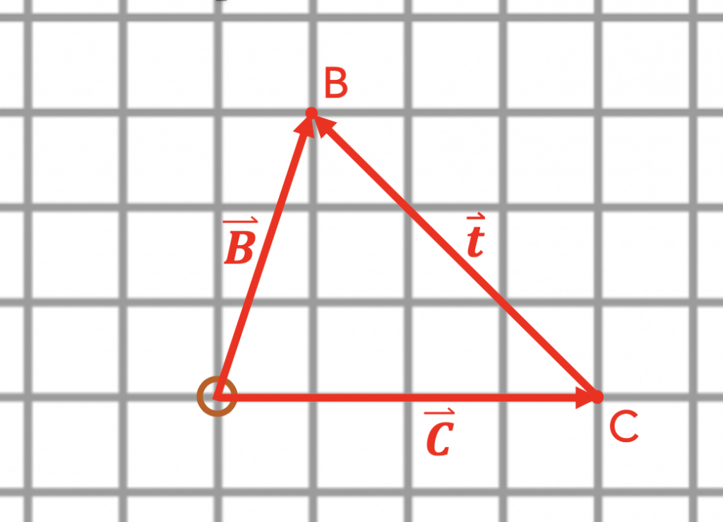
In the diagram below, you are standing at the origin (brown circle).  Your two friends Charlie (C) and Beth (B) are nearby.

Key Takeaways

Introductory Physics: Classical Mechanics Copyright © by . All Rights Reserved.

Share This Book

• school Campus Bookshelves
• menu_book Bookshelves
• perm_media Learning Objects
• login Login
• how_to_reg Request Instructor Account
• hub Instructor Commons
• Download Page (PDF)
• Download Full Book (PDF)
• Periodic Table
• Physics Constants
• Scientific Calculator
• Reference & Cite
• Tools expand_more
• Readability

selected template will load here

This action is not available.

1.6: Vector Addition

• Last updated
• Save as PDF
• Page ID 2822

Adding Vectors in Two Dimensions

In the following image, vectors A and B represent the two displacements of a person who walked 90. m east and then 50. m north. We want to add these two vectors to get the vector sum of the two movements.

The graphical process for adding vectors in two dimensions is to place the tail of the second vector on the arrow head of the first vector as shown above.

The sum of the two vectors is the vector that begins at the origin of the first vector and goes to the ending of the second vector, as shown below.

If we are using totally graphic means of adding these vectors, the magnitude of the sum can be determined by measuring the length of the sum vector and comparing it to the original standard. We then use a compass to measure the angle of the summation vector.

If we are using calculation, we first determine the inverse tangent of 50 units divided by 90 units and get the angle of 29° north of east. The length of the sum vector can then be determined mathematically by the Pythagorean theorem, a2+b2=c2. In this case, the length of the hypotenuse would be the square root of (8100 + 2500), or 103 units.

If three or four vectors are to be added by graphical means, we would continue to place each new vector head to toe with the vectors to be added until all the vectors were in the coordinate system. The resultant, or sum, vector would be the vector from the origin of the first vector to the arrowhead of the last vector; the magnitude and direction of this sum vector would then be measured.

Mathematical Methods of Vector Addition

We can add vectors mathematically using trig functions, the law of cosines, or the Pythagorean theorem.

If the vectors to be added are at right angles to each other, such as the example above, we would assign them to the sides of a right triangle and calculate the sum as the hypotenuse of the right triangle. We would also calculate the direction of the sum vector by using an inverse sin or some other trig function.

Suppose, however, that we wish to add two vectors that are not at right angles to each other. Let’s consider the vectors in the following images.

The two vectors we are to add are a force of 65 N at 30° north of east and a force of 35 N at 60° north of west.

We know that vectors in the same dimension can be added by regular arithmetic. Therefore, we can resolve each of these vectors into components that lay on the axes as pictured below. The resolution of vectors reduces each vector to a component on the north-south axis and a component on the east-west axis.

After resolving each vector into two components, we can now mathematically determine the magnitude of the components. Once we have done that, we can add the components in the same direction arithmetically. This will give us two vectors that are perpendicular to each other and can be the legs of a right triangle.

The east-west component of the first vector is (65 N)(cos 30°) = (65 N)(0.866) = 56.3 N north

The north-south component of the first vector is (65 N)(sin 30°) = (65 N)(0.500) = 32.5 N north

The east-west component of the second vector is (35 N)(cos 60°) = (35 N)(0.500) = 17.5 N west

The north-south component of the second vector is (35 N)(sin 60°) = (35 N)(0.866) = 30.3 N north

The sum of the two east-west components is 56.3 N - 17.5 N = 38.8 N east

The sum of the two north-south components is 32.5 N + 30.3 N = 62.8 N north

We can now consider those two vectors to be the sides of a right triangle and find the length and direction of the hypotenuse using the Pythagorean Theorem and trig functions.

c=38.82+62.82=74 N

sin⁡ x=62.874 so x=sin−1⁡0.84 so x=58∘

The direction of the sum vector is 74 N at 58° north of east.

Perpendicular vectors have no components in the other direction. For example, if a boat is floating down a river due south, and you are paddling the boat due east, the eastward vector has no component in the north-south direction and therefore, has no effect on the north-south motion. If the boat is floating down the river at 5 mph south and you paddle the boat eastward at 5 mph, the boat continues to float southward at 5 mph. The eastward motion has absolutely no effect on the southward motion. Perpendicular vectors have NO effect on each other.

A motorboat heads due east at 16 m/s across a river that flows due north at 9.0 m/s.

Example 1.6.1

What is the resultant velocity of the boat?

Since the two motions are perpendicular to each other, they can be assigned to the legs of a right triangle and the hypotenuse (resultant) calculated.

c=a2+b2=(16 m/s)2+(9.0 m/s)2=18 m/s

sin⁡θ=9.018=0.500 and therefore θ=30∘

The resultant is 18 m/s at 30° north of east.

Example 1.6.2

If the river is 135 m wide, how long does it take the boat to reach the other side?

The boat is traveling across the river at 16 m/s due to the motor. The current is perpendicular and therefore has no effect on the speed across the river. The time required for the trip can be determined by dividing the distance by the velocity.

t=dv=135 m16 m/s=8.4 s

Example 1.6.3

The boat is traveling across the river for 8.4 seconds and therefore, it is also traveling downstream for 8.4 seconds. We can determine the distance downstream the boat will travel by multiplying the speed downstream by the time of the trip.

d downstream =(v downstream )(t)=(9.0 m/s)(8.4 s)=76 m

Use this PLIX Interactive to visualize how any vector can be broken down into separate x and y components:

Interactive Element

• Vectors can be added mathematically using geometry and trigonometry.
• Vectors that are perpendicular to each other have no effect on each other.
• Vector addition can be accomplished by resolving the vectors to be added into components those vectors, and then completing the addition with the perpendicular components.
• What is the total distance walked by the hiker?
• What is the displacement (on a straight line) of the hiker from the camp?
• While flying due east at 33 m/s, an airplane is also being carried due north at 12 m/s by the wind. What is the plane’s resultant velocity?
• Two students push a heavy crate across the floor. John pushes with a force of 185 N due east and Joan pushes with a force of 165 N at 30° north of east. What is the resultant force on the crate?
• An airplane flying due north at 90. km/h is being blown due west at 50. km/h. What is the resultant velocity of the plane?

Explore More

Use this resource to answer the questions that follow.

• What are the steps the teacher undertakes in order to calculate the resultant vector in this problem?
• How does she find the components of the individual vectors?
• How does she use the individual vector’s components to find the components of the resultant vector?
• Once the components are determined, how does she find the overall resultant vector?

Additional Resources

Real World Application: Banked With No Friction

Vector Addition and Subtraction

• Two people are pushing a disabled car. One exerts a force of 200 N east, the other a force of 150 N east. What is the net force exerted on the car? (Assume friction to be negligible.)
• Two soccer players kick a ball simultaneously from opposite sides. Red #3 kicks with 50 N of force while Blue #5 kicks with 63 N of force. What is the net force on the ball?
• An airplane heads due north at 100 m/s through a 30 m/s cross wind blowing from the east to the west. Determine the resultant velocity of the airplane (relative to due north).
• A mountain climbing expedition establishes a base camp and two intermediate camps, A and B. Camp A is 11,200 m east of and 3,200 m above base camp. Camp B is 8400 m east of and 1700 m higher than Camp A. Determine the displacement between base camp and Camp B.
• A plane heads east with a velocity of 52 m/s through a 12 m/s cross wind blowing the plane south. Find the magnitude and direction of the plane's resultant velocity (relative to due east).
• An ambitious hiker walks 25 km west and then 35 km south in a day. Find the magnitude and direction of the hiker's resultant displacement (relative to due west).
• A boat heads directly across a river with a velocity of 12 m/s. If the river flows at 6.0 m/s find the magnitude and direction of the boat's resultant velocity. (State the direction relative to an imaginary line drawn straight across the river.)
• What distance did I travel?
• What's my resultant displacement (magnitude and direction relative to due east)?
• the bearing that the plane should take (relative to due north)
• the plane's speed with respect to the air
• At a particular instant, a stationary observer on the ground sees a package falling from a moving airplane with a speed v observer at an angle θ to the vertical. To the pilot flying horizontally at a constant speed relative to the ground the package appears to be falling vertically with a speed v pilot at that same instant. What is the speed of the pilot relative to the ground in terms of the given quantities?

graphical drill

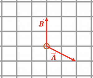
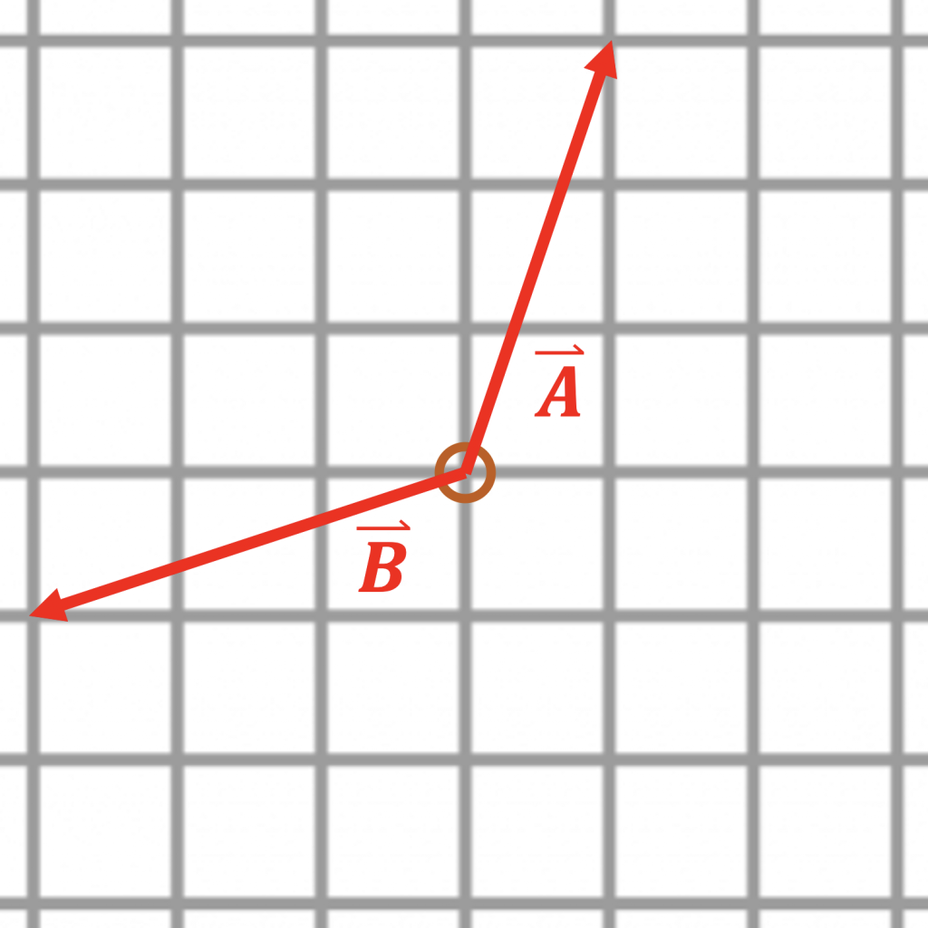
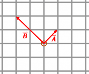
• worksheet-addition.pdf Determine the magnitude (in centimeters) and direction (in standard form) of the resultant vector B  +  A for each of the combinations below. Measure its length in centimeters and direction angle in standard form (i.e.; right 0°, up 90°, left 180°, down 270°, etc.). Use the horizontal reference lines as needed.
• worksheet-subtraction.pdf Determine the magnitude (in centimeters) and direction (in standard form) of the resultant vector B  −  A for each of the combinations below. Measure its length in centimeters and direction angle in standard form (i.e.; right 0°, up 90°, left 180°, down 270°, etc.). Use the horizontal reference lines as needed.

PHYS101: Introduction to Mechanics

Vector addition and subtraction.

As you read, pay attention to the worked examples: using the head-to-tail method to add multiple vectors in Example 3.1 and using the head-to-tail method to subtract vectors in Example 3.2.

Figure 3.8 Displacement can be determined graphically using a scale map, such as this one of the Hawaiian Islands. A journey from Hawai'i to Moloka'i has a number of legs, or journey segments. These segments can be added graphically with a ruler to determine the total two-dimensional displacement of the journey.

Vectors in Two Dimensions

A vector is a quantity that has magnitude and direction. Displacement, velocity, acceleration, and force, for example, are all vectors. In one-dimensional, or straight-line, motion, the direction of a vector can be given simply by a plus or minus sign. In two dimensions (2-d), however, we specify the direction of a vector relative to some reference frame (i.e., coordinate system), using an arrow having length proportional to the vector's magnitude and pointing in the direction of the vector.

Vectors in this Text

Vector Addition: Head-to-Tail Method

The head-to-tail method is a graphical way to add vectors, described in Figure 3.11 below and in the steps following. The tail of the vector is the starting point of the vector, and the head (or tip) of a vector is the final, pointed end of the arrow.

Step 1 . Draw an arrow to represent the first vector (9 blocks to the east) using a ruler and protractor.

Figure 3.12

Step 2 . Now draw an arrow to represent the second vector (5 blocks to the north). Place the tail of the second vector at the head of the first vector.

Figure 3.13

Step 3 . If there are more than two vectors, continue this process for each vector to be added. Note that in our example, we have only two vectors, so we have finished placing arrows tip to tail.

Step 4 . Draw an arrow from the tail of the first vector to the head of the last vector. This is the resultant, or the sum, of the other vectors.

Figure 3.14

Step 5 . To get the magnitude of the resultant, measure its length with a ruler. (Note that in most calculations, we will use the Pythagorean theorem to determine this length.)

Step 6 . To get the direction of the resultant, measure the angle it makes with the reference frame using a protractor. (Note that in most calculations, we will use trigonometric relationships to determine this angle.)

The graphical addition of vectors is limited in accuracy only by the precision with which the drawings can be made and the precision of the measuring tools. It is valid for any number of vectors.

Example 3.1 Adding Vectors Graphically Using the Head-to-Tail Method: A Woman Takes a Walk

(1) Draw the three displacement vectors.

Figure 3.15

(2) Place the vectors head to tail retaining both their initial magnitude and direction.

Figure 3.16

Figure 3.17

Figure 3.18

The head-to-tail graphical method of vector addition works for any number of vectors. It is also important to note that the resultant is independent of the order in which the vectors are added. Therefore, we could add the vectors in any order as illustrated in Figure 3.19 and we will still get the same solution.

Figure 3.19

Here, we see that when the same vectors are added in a different order, the result is the same. This characteristic is true in every case and is an important characteristic of vectors. Vector addition is commutative . Vectors can be added in any order.

Vector Subtraction

Example 3.2 Subtracting Vectors Graphically: A Woman Sailing a Boat

Figure 3.21

Figure 3.22

(2) Place the vectors head to tail.

Figure 3.23

Figure 3.24

We can see that the woman will end up a significant distance from the dock if she travels in the opposite direction for the second leg of the trip.

Because subtraction of a vector is the same as addition of a vector with the opposite direction, the graphical method of subtracting vectors works the same as for addition.

Multiplication of Vectors and Scalars

Resolving a vector into components.

In the examples above, we have been adding vectors to determine the resultant vector. In many cases, however, we will need to do the opposite. We will need to take a single vector and find what other vectors added together produce it. In most cases, this involves determining the perpendicular components of a single vector, for example the x- and y-components , or the north-south and east-west components.

• school Campus Bookshelves
• menu_book Bookshelves
• perm_media Learning Objects
• login Login
• how_to_reg Request Instructor Account
• hub Instructor Commons
• Download Page (PDF)
• Download Full Book (PDF)
• Periodic Table
• Physics Constants
• Scientific Calculator
• Reference & Cite
• Tools expand_more
• Readability

selected template will load here

This action is not available.

16.2: Vector Addition

• Last updated
• Save as PDF
• Page ID 55332

• Jacob Moore & Contributors
• Pennsylvania State University Mont Alto via Mechanics Map

The most common thing we will need to do with many vector quantities is to add them up. The sum of these vector quantities is the net vector quantity. For example, if we have a number of forces acting on a body, the sum of those forces is known as the net force.

The sum of any number of vectors can be determined geometrically using the following strategy. Starting with one of the vectors as the base, we redraw the second vector so that the tail of the second vector begins at the tip of the first vector. We can repeat this with a third vector, a forth vector and so on, putting the tail of each vector at the tip of the last vector until we have added taken all vectors into account. Once the vectors are all drawn tip to tail, the sum of all the vectors will be the vector connecting the tail of the first vector to the tip of the last vector.

In practice, the easiest way to determine the magnitude and direction of the sum of the vectors is to add the vectors in component form . This starts by separating each vector into \(x\), \(y\), and possibly \(z\) components. As we can see in the diagram below, the \(x\) component of the sum of all the vectors will be the sum of all the \(x\) components of the individual vectors. Similarly, the \(y\) and \(z\) components of the sum of the vectors will be the sum of all the \(y\) components and the sum of all the \(z\) components respectively.

Once we find the sum of the components in each direction, we can either leave the net vector in component form, or we can use the Pythagorean theorem and inverse tangent functions to convert the vector back into a magnitude and direction as detailed on the previous page on vectors .

Figure \(PageIndex{1}\): Vide lecture covering this section, delivered by Dr. Jacob Moore. YouTube source: https://youtu.be/0tv92MX2_ro .

Example \(\PageIndex{1}\)

Determine the sum of the force vectors in the diagram below. Leave the sum in component form.

Example \(\PageIndex{2}\)

Determine the sum of the force vectors in the diagram below. Give the sum in terms of a magnitude and a direction.

Example \(\PageIndex{3}\)

• TPC and eLearning
• Read Watch Interact
• What's NEW at TPC?
• Practice Review Test
• Teacher-Tools
• Subscription Selection
• Seat Calculator
• Ad Free Account
• Edit Profile Settings
• Classes (Version 2)
• Student Progress Edit
• Task Properties
• Export Student Progress
• Task, Activities, and Scores
• Metric Conversions Questions
• Metric System Questions
• Metric Estimation Questions
• Significant Digits Questions
• Proportional Reasoning
• Acceleration
• Distance-Displacement
• Dots and Graphs
• Graph That Motion
• Match That Graph
• Name That Motion
• Motion Diagrams
• Pos'n Time Graphs Numerical
• Pos'n Time Graphs Conceptual
• Up And Down - Questions
• Balanced vs. Unbalanced Forces
• Change of State
• Force and Motion
• Mass and Weight
• Match That Free-Body Diagram
• Net Force (and Acceleration) Ranking Tasks
• Newton's Second Law
• Normal Force Card Sort
• Recognizing Forces
• Air Resistance and Skydiving
• Solve It! with Newton's Second Law
• Which One Doesn't Belong?
• Component Addition Questions
• Head-to-Tail Vector Addition
• Projectile Mathematics
• Trajectory - Angle Launched Projectiles
• Trajectory - Horizontally Launched Projectiles
• Vector Addition
• Vector Direction
• Which One Doesn't Belong? Projectile Motion
• Forces in 2-Dimensions
• Being Impulsive About Momentum
• Explosions - Law Breakers
• Hit and Stick Collisions - Law Breakers
• Case Studies: Impulse and Force
• Impulse-Momentum Change Table
• Keeping Track of Momentum - Hit and Stick
• Keeping Track of Momentum - Hit and Bounce
• What's Up (and Down) with KE and PE?
• Energy Conservation Questions
• Energy Dissipation Questions
• Energy Ranking Tasks
• LOL Charts (a.k.a., Energy Bar Charts)
• Match That Bar Chart
• Words and Charts Questions
• Name That Energy
• Stepping Up with PE and KE Questions
• Case Studies - Circular Motion
• Circular Logic
• Forces and Free-Body Diagrams in Circular Motion
• Gravitational Field Strength
• Universal Gravitation
• Angular Position and Displacement
• Linear and Angular Velocity
• Angular Acceleration
• Rotational Inertia
• Balanced vs. Unbalanced Torques
• Getting a Handle on Torque
• Torque-ing About Rotation
• Properties of Matter
• Fluid Pressure
• Buoyant Force
• Sinking, Floating, and Hanging
• Pascal's Principle
• Flow Velocity
• Bernoulli's Principle
• Balloon Interactions
• Charge and Charging
• Charge Interactions
• Charging by Induction
• Conductors and Insulators
• Coulombs Law
• Electric Field
• Electric Field Intensity
• Polarization
• Case Studies: Electric Power
• Know Your Potential
• Light Bulb Anatomy
• I = ∆V/R Equations as a Guide to Thinking
• Parallel Circuits - ∆V = I•R Calculations
• Resistance Ranking Tasks
• Series Circuits - ∆V = I•R Calculations
• Series vs. Parallel Circuits
• Equivalent Resistance
• Period and Frequency of a Pendulum
• Pendulum Motion: Velocity and Force
• Energy of a Pendulum
• Period and Frequency of a Mass on a Spring
• Horizontal Springs: Velocity and Force
• Vertical Springs: Velocity and Force
• Energy of a Mass on a Spring
• Decibel Scale
• Frequency and Period
• Closed-End Air Columns
• Name That Harmonic: Strings
• Rocking the Boat
• Wave Basics
• Matching Pairs: Wave Characteristics
• Wave Interference
• Waves - Case Studies
• Color Addition and Subtraction
• Color Filters
• If This, Then That: Color Subtraction
• Light Intensity
• Color Pigments
• Converging Lenses
• Curved Mirror Images
• Law of Reflection
• Refraction and Lenses
• Total Internal Reflection
• Who Can See Who?
• Formulas and Atom Counting
• Atomic Models
• Bond Polarity
• Entropy Questions
• Cell Voltage Questions
• Heat of Formation Questions
• Reduction Potential Questions
• Oxidation States Questions
• Measuring the Quantity of Heat
• Hess's Law
• Oxidation-Reduction Questions
• Galvanic Cells Questions
• Thermal Stoichiometry
• Molecular Polarity
• Quantum Mechanics
• Balancing Chemical Equations
• Bronsted-Lowry Model of Acids and Bases
• Classification of Matter
• Collision Model of Reaction Rates
• Density Ranking Tasks
• Dissociation Reactions
• Complete Electron Configurations
• Elemental Measures
• Enthalpy Change Questions
• Equilibrium Concept
• Equilibrium Constant Expression
• Equilibrium Calculations - Questions
• Equilibrium ICE Table
• Intermolecular Forces Questions
• Ionic Bonding
• Lewis Electron Dot Structures
• Limiting Reactants
• Line Spectra Questions
• Mass Stoichiometry
• Measurement and Numbers
• Metals, Nonmetals, and Metalloids
• Metric Estimations
• Metric System
• Molarity Ranking Tasks
• Mole Conversions
• Name That Element
• Names to Formulas
• Names to Formulas 2
• Nuclear Decay
• Particles, Words, and Formulas
• Periodic Trends
• Precipitation Reactions and Net Ionic Equations
• Pressure Concepts
• Pressure-Temperature Gas Law
• Pressure-Volume Gas Law
• Chemical Reaction Types
• Significant Digits and Measurement
• States Of Matter Exercise
• Stoichiometry Law Breakers
• Stoichiometry - Math Relationships
• Subatomic Particles
• Spontaneity and Driving Forces
• Gibbs Free Energy
• Volume-Temperature Gas Law
• Acid-Base Properties
• Energy and Chemical Reactions
• Chemical and Physical Properties
• Valence Shell Electron Pair Repulsion Theory
• Writing Balanced Chemical Equations
• Mission CG1
• Mission CG10
• Mission CG2
• Mission CG3
• Mission CG4
• Mission CG5
• Mission CG6
• Mission CG7
• Mission CG8
• Mission CG9
• Mission EC1
• Mission EC10
• Mission EC11
• Mission EC12
• Mission EC2
• Mission EC3
• Mission EC4
• Mission EC5
• Mission EC6
• Mission EC7
• Mission EC8
• Mission EC9
• Mission RL1
• Mission RL2
• Mission RL3
• Mission RL4
• Mission RL5
• Mission RL6
• Mission KG7
• Mission RL8
• Mission KG9
• Mission RL10
• Mission RL11
• Mission RM1
• Mission RM2
• Mission RM3
• Mission RM4
• Mission RM5
• Mission RM6
• Mission RM8
• Mission RM10
• Mission LC1
• Mission RM11
• Mission LC2
• Mission LC3
• Mission LC4
• Mission LC5
• Mission LC6
• Mission LC8
• Mission SM1
• Mission SM2
• Mission SM3
• Mission SM4
• Mission SM5
• Mission SM6
• Mission SM8
• Mission SM10
• Mission KG10
• Mission SM11
• Mission KG2
• Mission KG3
• Mission KG4
• Mission KG5
• Mission KG6
• Mission KG8
• Mission KG11
• Mission F2D1
• Mission F2D2
• Mission F2D3
• Mission F2D4
• Mission F2D5
• Mission F2D6
• Mission KC1
• Mission KC2
• Mission KC3
• Mission KC4
• Mission KC5
• Mission KC6
• Mission KC7
• Mission KC8
• Mission AAA
• Mission SM9
• Mission LC7
• Mission LC9
• Mission NL1
• Mission NL2
• Mission NL3
• Mission NL4
• Mission NL5
• Mission NL6
• Mission NL7
• Mission NL8
• Mission NL9
• Mission NL10
• Mission NL11
• Mission NL12
• Mission MC1
• Mission MC10
• Mission MC2
• Mission MC3
• Mission MC4
• Mission MC5
• Mission MC6
• Mission MC7
• Mission MC8
• Mission MC9
• Mission RM7
• Mission RM9
• Mission RL7
• Mission RL9
• Mission SM7
• Mission SE1
• Mission SE10
• Mission SE11
• Mission SE12
• Mission SE2
• Mission SE3
• Mission SE4
• Mission SE5
• Mission SE6
• Mission SE7
• Mission SE8
• Mission SE9
• Mission VP1
• Mission VP10
• Mission VP2
• Mission VP3
• Mission VP4
• Mission VP5
• Mission VP6
• Mission VP7
• Mission VP8
• Mission VP9
• Mission WM1
• Mission WM2
• Mission WM3
• Mission WM4
• Mission WM5
• Mission WM6
• Mission WM7
• Mission WM8
• Mission WE1
• Mission WE10
• Mission WE2
• Mission WE3
• Mission WE4
• Mission WE5
• Mission WE6
• Mission WE7
• Mission WE8
• Mission WE9
• Vector Walk Interactive
• Name That Motion Interactive
• Kinematic Graphing 1 Concept Checker
• Kinematic Graphing 2 Concept Checker
• Graph That Motion Interactive
• Two Stage Rocket Interactive
• Rocket Sled Concept Checker
• Force Concept Checker
• Free-Body Diagrams Concept Checker
• Free-Body Diagrams The Sequel Concept Checker
• Skydiving Concept Checker
• Elevator Ride Concept Checker
• Vector Addition Concept Checker
• Vector Walk in Two Dimensions Interactive
• Name That Vector Interactive
• River Boat Simulator Concept Checker
• Projectile Simulator 2 Concept Checker
• Projectile Simulator 3 Concept Checker
• Hit the Target Interactive
• Turd the Target 1 Interactive
• Turd the Target 2 Interactive
• Balance It Interactive
• Go For The Gold Interactive
• Egg Drop Concept Checker
• Fish Catch Concept Checker
• Exploding Carts Concept Checker
• Collision Carts - Inelastic Collisions Concept Checker
• Its All Uphill Concept Checker
• Stopping Distance Concept Checker
• Chart That Motion Interactive
• Roller Coaster Model Concept Checker
• Uniform Circular Motion Concept Checker
• Horizontal Circle Simulation Concept Checker
• Vertical Circle Simulation Concept Checker
• Race Track Concept Checker
• Gravitational Fields Concept Checker
• Orbital Motion Concept Checker
• Angular Acceleration Concept Checker
• Balance Beam Concept Checker
• Torque Balancer Concept Checker
• Aluminum Can Polarization Concept Checker
• Charging Concept Checker
• Name That Charge Simulation
• Coulomb's Law Concept Checker
• Electric Field Lines Concept Checker
• Put the Charge in the Goal Concept Checker
• Circuit Builder Concept Checker (Series Circuits)
• Circuit Builder Concept Checker (Parallel Circuits)
• Circuit Builder Concept Checker (∆V-I-R)
• Circuit Builder Concept Checker (Voltage Drop)
• Equivalent Resistance Interactive
• Pendulum Motion Simulation Concept Checker
• Mass on a Spring Simulation Concept Checker
• Particle Wave Simulation Concept Checker
• Boundary Behavior Simulation Concept Checker
• Slinky Wave Simulator Concept Checker
• Simple Wave Simulator Concept Checker
• Wave Addition Simulation Concept Checker
• Standing Wave Maker Simulation Concept Checker
• Color Addition Concept Checker
• Painting With CMY Concept Checker
• Stage Lighting Concept Checker
• Filtering Away Concept Checker
• InterferencePatterns Concept Checker
• Young's Experiment Interactive
• Plane Mirror Images Interactive
• Who Can See Who Concept Checker
• Optics Bench (Mirrors) Concept Checker
• Name That Image (Mirrors) Interactive
• Refraction Concept Checker
• Total Internal Reflection Concept Checker
• Optics Bench (Lenses) Concept Checker
• Kinematics Preview
• Velocity Time Graphs Preview
• Moving Cart on an Inclined Plane Preview
• Stopping Distance Preview
• Cart, Bricks, and Bands Preview
• Fan Cart Study Preview
• Friction Preview
• Coffee Filter Lab Preview
• Friction, Speed, and Stopping Distance Preview
• Up and Down Preview
• Projectile Range Preview
• Ballistics Preview
• Juggling Preview
• Marshmallow Launcher Preview
• Air Bag Safety Preview
• Colliding Carts Preview
• Collisions Preview
• Engineering Safer Helmets Preview
• Push the Plow Preview
• Its All Uphill Preview
• Energy on an Incline Preview
• Modeling Roller Coasters Preview
• Hot Wheels Stopping Distance Preview
• Ball Bat Collision Preview
• Energy in Fields Preview
• Weightlessness Training Preview
• Roller Coaster Loops Preview
• Universal Gravitation Preview
• Keplers Laws Preview
• Kepler's Third Law Preview
• Charge Interactions Preview
• Sticky Tape Experiments Preview
• Wire Gauge Preview
• Voltage, Current, and Resistance Preview
• Light Bulb Resistance Preview
• Series and Parallel Circuits Preview
• Thermal Equilibrium Preview
• Linear Expansion Preview
• Heating Curves Preview
• Electricity and Magnetism - Part 1 Preview
• Electricity and Magnetism - Part 2 Preview
• Vibrating Mass on a Spring Preview
• Period of a Pendulum Preview
• Wave Speed Preview
• Slinky-Experiments Preview
• Standing Waves in a Rope Preview
• Sound as a Pressure Wave Preview
• DeciBel Scale Preview
• DeciBels, Phons, and Sones Preview
• Sound of Music Preview
• Shedding Light on Light Bulbs Preview
• Models of Light Preview
• Electromagnetic Radiation Preview
• Electromagnetic Spectrum Preview
• EM Wave Communication Preview
• Digitized Data Preview
• Light Intensity Preview
• Concave Mirrors Preview
• Object Image Relations Preview
• Snells Law Preview
• Reflection vs. Transmission Preview
• Magnification Lab Preview
• Reactivity Preview
• Ions and the Periodic Table Preview
• Periodic Trends Preview
• Intermolecular Forces Preview
• Melting Points and Boiling Points Preview
• Reaction Rates Preview
• Ammonia Factory Preview
• Stoichiometry Preview
• Nuclear Chemistry Preview
• Gaining Teacher Access
• Tasks and Classes
• Tasks - Classic
• Subscription
• Subscription Locator
• 1-D Kinematics
• Newton's Laws
• Vectors - Motion and Forces in Two Dimensions
• Momentum and Its Conservation
• Work and Energy
• Circular Motion and Satellite Motion
• Thermal Physics
• Static Electricity
• Electric Circuits
• Vibrations and Waves
• Sound Waves and Music
• Light and Color
• Reflection and Mirrors
• About the Physics Interactives
• Task Tracker
• Usage Policy
• Newtons Laws
• Vectors and Projectiles
• Forces in 2D
• Momentum and Collisions
• Circular and Satellite Motion
• Balance and Rotation
• Electromagnetism
• Waves and Sound
• Atomic Physics
• Forces in Two Dimensions
• Work, Energy, and Power
• Circular Motion and Gravitation
• Sound Waves
• 1-Dimensional Kinematics
• Circular, Satellite, and Rotational Motion
• Einstein's Theory of Special Relativity
• Waves, Sound and Light
• QuickTime Movies
• About the Concept Builders
• Pricing For Schools
• Directions for Version 2
• Measurement and Units
• Relationships and Graphs
• Rotation and Balance
• Vibrational Motion
• Reflection and Refraction
• Teacher Accounts
• Task Tracker Directions
• Kinematic Concepts
• Kinematic Graphing
• Wave Motion
• Sound and Music
• About CalcPad
• 1D Kinematics
• Vectors and Forces in 2D
• Simple Harmonic Motion
• Rotational Kinematics
• Rotation and Torque
• Rotational Dynamics
• Electric Fields, Potential, and Capacitance
• Transient RC Circuits
• Light Waves
• Units and Measurement
• Stoichiometry
• Molarity and Solutions
• Thermal Chemistry
• Acids and Bases
• Kinetics and Equilibrium
• Solution Equilibria
• Oxidation-Reduction
• Nuclear Chemistry
• NGSS Alignments
• 1D-Kinematics
• Projectiles
• Circular Motion
• Magnetism and Electromagnetism
• Graphing Practice
• About the ACT
• ACT Preparation
• For Teachers
• Other Resources
• Newton's Laws of Motion
• Work and Energy Packet
• Static Electricity Review
• Solutions Guide
• Solutions Guide Digital Download
• Motion in One Dimension
• Work, Energy and Power
• Frequently Asked Questions
• Purchasing the Download
• Purchasing the CD
• Purchasing the Digital Download
• About the NGSS Corner
• NGSS Search
• Force and Motion DCIs - High School
• Energy DCIs - High School
• Wave Applications DCIs - High School
• Force and Motion PEs - High School
• Energy PEs - High School
• Wave Applications PEs - High School
• Crosscutting Concepts
• The Practices
• Physics Topics
• NGSS Corner: Activity List
• NGSS Corner: Infographics
• About the Toolkits
• Position-Velocity-Acceleration
• Position-Time Graphs
• Velocity-Time Graphs
• Newton's First Law
• Newton's Second Law
• Newton's Third Law
• Terminal Velocity
• Projectile Motion
• Forces in 2 Dimensions
• Impulse and Momentum Change
• Momentum Conservation
• Work-Energy Fundamentals
• Work-Energy Relationship
• Roller Coaster Physics
• Satellite Motion
• Electric Fields
• Circuit Concepts
• Series Circuits
• Parallel Circuits
• Describing-Waves
• Wave Behavior Toolkit
• Standing Wave Patterns
• Resonating Air Columns
• Wave Model of Light
• Plane Mirrors
• Curved Mirrors
• Teacher Guide
• Using Lab Notebooks
• Current Electricity
• Light Waves and Color
• Reflection and Ray Model of Light
• Refraction and Ray Model of Light
• Classes (Legacy Version)
• Teacher Resources
• Subscriptions

• Newton's Laws
• Einstein's Theory of Special Relativity
• About Concept Checkers
• School Pricing
• Newton's Laws of Motion
• Newton's First Law
• Newton's Third Law

Teaching Ideas and Suggestions:

Related resources.

• Reading: Lessons 1 of the Motion in Two-Dimensions Chapter of the Tutorial are perfect accompaniments to this Interactive. The following pages will be particularly useful in understanding component addition: Vector A ddition Resultants Vector Components Vector Resolution Component Addition
• Minds On Physics Internet Modules: The Minds On Physics Internet Modules include a collection of interactive questioning modules that help learners assess their understanding of physics concepts and solidify those understandings by answering questions that require higher-order thinking. Assignments VP2, VP3, VP4, and VP5 of the Vectors and Projectiles module provide great complements to this Interactive. They are best used in the middle to later stages of the learning cycle. Visit the  Minds On Physics Internet Modules .  
• Curriculum/Practice: Several Concept Development worksheets at the Curriculum Corner will be very useful in assisting students in cultivating their understanding, most notably ... Addition of Vectors Vector Components, Vector Resolution and Vector Addition Vector Addition by Components Visit the  Curriculum Corner .  
• Labwork:  Simulations should always support (never replace) hands-on learning. The Laboratory section of The Physics Classroom website includes several hands-on ideas that complement this Interactive. Four notable lab ides include ... Map Lab As the Crow Flies Lab Where Am I? Lab Road Trip Lab Visit The Laboratory .