non parametric test research

LEARN STATISTICS EASILY

Learn Data Analysis Now!

Non-Parametric Statistics: A Comprehensive Guide

Exploring the Versatile World of Non-Parametric Statistics: Mastering Flexible Data Analysis Techniques.

Introduction

Non-parametric statistics  serve as a critical toolset in data analysis. They are known for their adaptability and the capacity to provide valid results without the stringent prerequisites demanded by parametric counterparts. This article delves into the fundamentals of non-parametric techniques, shedding light on their operational mechanisms, advantages, and scenarios of optimal application. By equipping readers with a solid grasp of  non-parametric statistics , we aim to enhance their analytical capabilities, enabling the effective handling of diverse datasets, especially those that challenge conventional parametric assumptions. Through a precise, technical exposition, this guide seeks to elevate the reader’s proficiency in applying non-parametric methods to extract meaningful insights from data, irrespective of its distribution or scale.

• Non-parametric statistics bypass assumptions for true data integrity.
• Flexible methods in non-parametric statistics reveal hidden data patterns.
• Real-world applications of non-parametric statistics solve complex issues.
• Non-parametric techniques like Mann-Whitney U bring clarity to data.
• Ethical data analysis through non-parametric statistics upholds truth.

Ad description. Lorem ipsum dolor sit amet, consectetur adipiscing elit.

Understanding Non-Parametric Statistics

Non-parametric statistics  are indispensable in data analysis, mainly due to their capacity to process data without the necessity for predefined distribution assumptions. This distinct attribute sets non-parametric methods apart from parametric ones, which mandate that data adhere to certain distribution norms, such as the normal distribution. The utility of non-parametric techniques becomes especially pronounced with datasets where the distribution is either unknown, non-normal, or insufficient sample size to validate any distributional assumptions.

The cornerstone of  non-parametric statistics  is their reliance on the ranks or order of data points instead of the actual data values. This approach renders them inherently resilient to outliers and aptly suited for analyzing non-linear relationships within the data. Such versatility makes non-parametric methods applicable across diverse data types and research contexts, including situations involving ordinal data or instances where scale measurements are infeasible.

By circumventing the assumption of a specific underlying distribution, non-parametric methods facilitate a more authentic data analysis, capturing its intrinsic structure and characteristics. This capability allows researchers to derive conclusions that are more aligned with the actual nature of their data, which is particularly beneficial in disciplines where data may not conform to the conventional assumptions underpinning parametric tests.

Non-Parametric Statistics Flexibility

The core advantage of Non-Parametric Statistics lies in its inherent flexibility, which is crucial for analyzing data that doesn’t conform to the assumptions required by traditional parametric methods. This flexibility stems from the ability of non-parametric techniques to make fewer assumptions about the data distribution, allowing for a broader application across various types of data structures and distributions.

For instance, non-parametric methods do not assume a specific underlying distribution (such as normal distribution), making them particularly useful for skewed, outliers, or ordinal data. This is a significant technical benefit when dealing with real-world data, often deviating from idealized statistical assumptions.

Moreover, non-parametric statistics are adept at handling small sample sizes where the central limit theorem might not apply, and parametric tests could be unreliable. This makes them invaluable in fields where large samples are difficult to obtain, such as in rare disease research or highly specialized scientific studies.

Another technical aspect of non-parametric methods is their use in hypothesis testing, particularly with the Wilcoxon Signed-Rank Test for paired data and the Mann-Whitney U Test for independent samples. These tests are robust alternatives to the t-test when the data does not meet the necessary parametric assumptions, providing a means to conduct meaningful statistical analysis without the stringent requirements of normality and homoscedasticity.

The flexibility of non-parametric methods extends to their application in correlation analysis with Spearman’s rank correlation and in estimating distribution functions with the Kaplan-Meier estimator, among others. These tools are indispensable in fields ranging from medical research to environmental studies, where the nature of the data and the research questions do not fit neatly into parametric frameworks.

Techniques and Methods

In  non-parametric statistics , several essential techniques and methods stand out for their utility and versatility across various types of data analysis. This section delves into six standard non-parametric tests, providing a technical overview of each method and its application.

Mann-Whitney U Test : Often employed as an alternative to the t-test for independent samples, the Mann-Whitney U test is pivotal when comparing two independent groups. It assesses whether their distributions differ significantly, relying not on the actual data values but on the ranks of these values. This test is instrumental when the data doesn’t meet the normality assumption required by parametric tests.

Wilcoxon Signed-Rank Test : This test is a non-parametric alternative to the paired t-test, used when assessing the differences between two related samples, matched samples, or repeated measurements on a single sample. The Wilcoxon test evaluates whether the median differences between pairs of observations are zero. It is ideal for the paired differences that do not follow a normal distribution.

Kruskal-Wallis Test : As the non-parametric counterpart to the one-way ANOVA, the Kruskal-Wallis test extends the Mann-Whitney U test to more than two independent groups. It evaluates whether the populations from which the samples are drawn have identical distributions. Like the Mann-Whitney U, it bases its analysis on the rank of the data, making it suitable for data that does not follow a normal distribution.

Friedman Test : Analogous to the repeated measures ANOVA in parametric statistics, the Friedman test is a non-parametric method for detecting differences in treatments across multiple test attempts. It is beneficial for analyzing data from experiments where measurements are taken from the same subjects under different conditions, allowing for assessing the effects of other treatments on a single sample population.

Spearman’s Rank Correlation : Spearman’s rank correlation coefficient offers a non-parametric measure of the strength and direction of association between two variables. It is especially applicable in scenarios where the variables are measured on an ordinal scale or when the relationship between variables is not linear. This method emphasizes the monotonic relationship between variables, providing insights into the data’s behavior beyond linear correlations.

Kendall’s Tau : Kendall’s Tau is a correlation measure designed to assess the association between two measured quantities. It determines the strength and direction of the relationship, much like Spearman’s rank correlation, but focuses on the concordance and discordance between data points. Kendall’s Tau is particularly useful for data that involves ordinal or ranked variables, providing insight into the monotonic relationship without assuming linearity.

Chi-square Test:  The Chi-square test is a non-parametric statistical tool used to determine whether there is a significant difference between the expected frequencies and the observed frequencies in one or more categories. It is beneficial in categorical data analysis, where the variables are nominal or ordinal, and the data are in the form of frequencies or counts. This test is valuable when evaluating hypotheses on the independence of two variables or the goodness of fit for a particular distribution.

Non-Parametric Statistics Real-World Applications

The practical utility of  Non-Parametric Statistics  is vast and varied, spanning numerous fields and research disciplines. This section showcases real-world case studies and examples where non-parametric methods have provided insightful solutions to complex problems, highlighting the depth and versatility of these techniques.

Environmental Science : In a study examining the impact of industrial pollution on river water quality, researchers employed the Kruskal-Wallis test to compare the pH levels across multiple sites. This non-parametric method was chosen due to the non-normal distribution of pH levels and the presence of outliers caused by sporadic pollution events. The test revealed significant differences in water quality, guiding policymakers in identifying pollution hotspots.

Medical Research : In a longitudinal study on chronic pain management, the Wilcoxon Signed-Rank Test was employed to assess the effectiveness of a novel therapy compared to conventional treatment. Each patient underwent both treatments in different periods, with pain scores recorded on an ordinal scale before and after each treatment phase. Given the non-normal distribution of differences in pain scores before and after each treatment for the same patient, the Wilcoxon test facilitated a statistically robust analysis. It revealed a significant reduction in pain intensity with the new therapy compared to conventional treatment, thereby demonstrating its superior efficacy in a manner that was both robust and suited to the paired nature of the data.

Market Research : A market research firm used Spearman’s Rank Correlation to analyze survey data to understand customer satisfaction across various service sectors. The ordinal ranking of satisfaction levels and the non-linear relationship between service features and customer satisfaction made Spearman’s correlation an ideal choice, uncovering critical drivers of customer loyalty.

Education : In educational research, the Friedman test was utilized to assess the effectiveness of different teaching methods on student performance over time. With data collected from the same group of students under three distinct teaching conditions, the test provided insights into which method led to significant improvements, informing curriculum development.

Social Sciences : Kendall’s Tau was applied in a sociological study to examine the relationship between social media usage and community engagement among youths. Given the ordinal data and the interest in understanding the direction and strength of the association without assuming linearity, Kendall’s Tau offered nuanced insights, revealing a weak but significant negative correlation.

Non-Parametric Statistics Implementation in R

Implementing non-parametric statistical methods in R involves a systematic approach to ensure accurate and ethical analysis. This step-by-step guide will walk you through the process, from data preparation to result interpretation, while emphasizing the importance of data integrity and ethical considerations.

1. Data Preparation:

• Begin by importing your dataset into R using functions like read.csv() for CSV files or read.table() for tab-delimited data.
• Perform initial data exploration using functions like summary(), str(), and head() to understand your data’s structure, variables, and any apparent issues like missing values or outliers.

2. Choosing the Right Test:

• Determine the appropriate non-parametric test based on your data type and research question. For two independent samples, consider the Mann-Whitney U test (wilcox.test() function); for paired samples, use the Wilcoxon Signed-Rank test (wilcox.test() with paired = TRUE); for more than two independent groups, use the Kruskal-Wallis test (kruskal.test()); and for correlation analysis, use Spearman’s rank correlation (cor.test() with method = “spearman”).

3. Executing the Test:

• Execute the chosen test using its corresponding function. Ensure your data meets the test’s requirements, such as correctly ranked or categorized.
• For example, to run a Mann-Whitney U test, use wilcox.test(group1, group2), replacing group1 and group2 with your actual data vectors.

4. Result Interpretation:

• Carefully interpret the output, paying attention to the test statistic and p-value. A p-value less than your significance level (commonly 0.05) indicates a statistically significant difference or correlation.
• Consider the effect size and confidence intervals to assess the practical significance of your findings.

5. Data Integrity and Ethical Considerations:

• Ensure data integrity by double-checking data entry, handling missing values appropriately, and conducting outlier analysis.
• Maintain ethical standards by respecting participant confidentiality, obtaining necessary permissions for data use, and reporting findings honestly without data manipulation.

6. Reporting:

• When documenting your analysis, include a detailed methodology section that outlines the non-parametric tests used, reasons for their selection, and any data preprocessing steps.
• Present your results using visual aids like plots or tables where applicable, and discuss the implications of your findings in the context of your research question.

Throughout this article, we have underscored the significance and value of  non-parametric statistics  in data analysis. These methods enable us to approach data sets with unknown or non-normal distributions, providing genuine insights and unveiling the truth and beauty hidden within the data. We encourage readers to maintain an  open mind  and a steadfast commitment to uncovering authentic insights when applying statistical methods to their research and projects. We invite you to explore the potential of  non-parametric statistics  in your endeavors and to share your findings with the scientific and academic community, contributing to the collective enrichment of knowledge and the advancement of science.

Recommended Articles

Discover more about the transformative power of data analysis in our collection of articles. Dive deeper into the world of statistics with our curated content and join our community of truth-seeking analysts.

Understanding the Assumptions for Chi-Square Test of Independence

• What is the difference between t-test and Mann-Whitney test?
• Mastering the Mann-Whitney U Test: A Comprehensive Guide
• A Comprehensive Guide to Hypotheses Tests in Statistics
• A Guide to Hypotheses Tests

Frequently Asked Questions (FAQs)

Q1: What Are Non-Parametric Statistics?  Non-parametric statistics are methods that don’t rely on data from specific distributions. They are used when data doesn’t meet the assumptions of parametric tests.

Q2: Why Choose Non-Parametric Methods?  They offer flexibility in analyzing data with unknown distributions or small sample sizes, providing a more ethical approach to data analysis.

Q3: What Is the Mann-Whitney U Test?  It’s a non-parametric test for assessing whether two independent samples come from the same distribution, especially useful when data doesn’t meet normality assumptions.

Q4: How Do Non-Parametric Methods Enhance Data Integrity?  By not imposing strict assumptions on data, non-parametric methods respect the natural form of data, leading to more truthful insights.

Q5: Can Non-Parametric Statistics Handle Outliers?  Yes, non-parametric statistics are less sensitive to outliers, making them suitable for datasets with extreme values.

Q6: What Is the Kruskal-Wallis Test?  This test is a non-parametric method for comparing more than two independent samples, proper when the ANOVA assumptions are not met.

Q7: How Does Spearman’s Rank Correlation Work?  Spearman’s rank correlation measures the strength and direction of association between two ranked variables, ideal for non-linear relationships.

Q8: What Are the Real-World Applications of Non-Parametric Statistics?  They are widely used in fields like environmental science, education, and medicine, where data may not follow standard distributions.

Q9: What Are the Benefits of Using Non-Parametric Statistics in Data Analysis?  They provide a more inclusive data analysis, accommodating various data types and distributions and revealing deeper insights.

Q10: How to Get Started with Non-Parametric Statistical Analysis?  Begin by understanding the nature of your data and choosing appropriate non-parametric methods that align with your analysis goals.

Similar Posts

How Do You Calculate Degrees of Freedom?

Master “How do you calculate degrees of freedom” in statistical analysis to enhance data accuracy and insights.

ANOVA versus ANCOVA: Breaking Down the Differences

Explore the crucial differences between ANOVA versus ANCOVA, and learn when to use each method for optimal data analysis.

“What Does The P-Value Mean” Revisited

We Have Already Presented A Didactic Explanation Of The P-Value, But Not That Precise. Now Learn An Accurate Definition For The P-Value!

What’s Regression Analysis? A Comprehensive Guide for Beginners

Discover what’s regression analysis, its types, key concepts, applications, and common pitfalls in our comprehensive guide for beginners.

Explore the assumptions and applications of the Chi-Square Test of Independence, a crucial tool for analyzing categorical data in various fields.

How to Report Simple Linear Regression Results in APA Style

With this article, you will learn How to Report Simple Linear Regression in APA-style. Ensure accurate, credible research results.

Leave a Reply Cancel reply

Your email address will not be published. Required fields are marked *

Save my name, email, and website in this browser for the next time I comment.

Thank you for visiting nature.com. You are using a browser version with limited support for CSS. To obtain the best experience, we recommend you use a more up to date browser (or turn off compatibility mode in Internet Explorer). In the meantime, to ensure continued support, we are displaying the site without styles and JavaScript.

• View all journals
• Explore content
• About the journal
• Publish with us
• Sign up for alerts
• Published: 29 April 2014

Points of significance

Nonparametric tests

• Martin Krzywinski 1 &
• Naomi Altman 2  

Nature Methods volume  11 ,  pages 467–468 ( 2014 ) Cite this article

64k Accesses

54 Citations

13 Altmetric

Metrics details

• Research data
• Statistical methods

A Corrigendum to this article was published on 27 June 2014

This article has been updated

Nonparametric tests robustly compare skewed or ranked data.

You have full access to this article via your institution.

We have seen that the t -test is robust with respect to assumptions about normality and equivariance 1 and thus is widely applicable. There is another class of methods—nonparametric tests—more suitable for data that come from skewed distributions or have a discrete or ordinal scale. Nonparametric tests such as the sign and Wilcoxon rank-sum tests relax distribution assumptions and are therefore easier to justify, but they come at the cost of lower sensitivity owing to less information inherent in their assumptions. For small samples, the performance of these tests is also constrained because their P values are only coarsely sampled and may have a large minimum. Both issues are mitigated by using larger samples.

These tests work analogously to their parametric counterparts: a test statistic and its distribution under the null are used to assign significance to observations. We compare in Figure 1 the one-sample t -test 2 to a nonparametric equivalent, the sign test (though more sensitive and sophisticated variants exist), using a putative sample X whose source distribution we cannot readily identify ( Fig. 1a ). The null hypothesis of the sign test is that the sample median m X is equal to the proposed median, M = 0.4. The test uses the number of sample values larger than M as its test statistic, W —under the null we expect to see as many values below the median as above, with the exact probability given by the binomial distribution ( Fig. 1c ). The median is a more useful descriptor than the mean for asymmetric and otherwise irregular distributions. The sign test makes no assumptions about the distribution—only that sample values be independent. If we propose that the population median is M = 0.4 and we observe X , we find W = 5 ( Fig. 1b ). The chance of observing a value of W under the null that is at least as extreme ( W ≤ 1 or W ≥ 5) is P = 0.22, using both tails of the binomial distribution ( Fig. 1c ). To limit the test to whether the median of X was biased towards values larger than M , we would consider only the area for W ≥ 5 in the right tail to find P = 0.11.

The P value of 0.22 from the sign test is much higher than that from the t -test ( P = 0.04), reflecting that the sign test is less sensitive. This is because it is not influenced by the actual distance between the sample values and M —it measures only 'how many' instead of 'how much'. Consequently, it needs larger sample sizes or more supporting evidence than the t -test. For the example of X , to obtain P < 0.05 we would need to have all values larger than M ( W = 6). Its large P values and straightforward application makes the sign test a useful diagnostic. Take, for example, a hypothetical situation slightly different from that in Figure 1 , where P > 0.05 is reported for the case where a treatment has lowered blood pressure in 6 out of 6 subjects. You may think this P seems implausibly large, and you'd be right because the equivalent scenario for the sign test ( W = 6, n = 6) gives a two-tailed P = 0.03.

To compare two samples, the Wilcoxon rank-sum test is widely used and is sometimes referred to as the Mann-Whitney or Mann-Whitney-Wilcoxon test. It tests whether the samples come from distributions with the same median. It doesn't assume normality, but as a test of equality of medians, it requires both samples to come from distributions with the same shape. The Wilcoxon test is one of many methods that reduce the dynamic range of values by converting them to their ranks in the list of ordered values pooled from both samples ( Fig. 2a ). The test statistic, W , is the degree to which the sum of ranks is larger than the lowest possible in the sample with the lower ranks ( Fig. 2b ). We expect that a sample from a population with a smaller median will be converted to a set of smaller ranks.

( a ) Sample comparisons of X vs. Y and X vs. Z start with ranking pooled values and identifying the ranks in the smaller-sized sample (e.g., 1, 3, 4, 5 for Y ; 1, 2, 3, 6 for Z ). Error bars show sample mean and s.d., and sample medians are shown by vertical dotted lines. ( b ) The Wilcoxon rank-sum test statistic W is the difference between the sum of ranks and the smallest possible observed sum. ( c ) For small sample sizes the exact distribution of W can be calculated. For samples of size (6, 4), there are only 210 different rank combinations corresponding to 25 distinct values of W .

Because there is a finite number (210) of combinations of rank-ordering for X ( n X = 6) and Y ( n Y = 4), we can enumerate all outcomes of the test and explicitly construct the distribution of W ( Fig. 2c ) to assign a P value to W . The smallest value of W = 0 occurs when all values in one sample are smaller than those in the other. When they are all larger, the statistic reaches a maximum, W = n X n Y = 24. For X versus Y , W = 3, and there are 14 of 210 test outcomes with W ≤ 3 or W ≥ 21. Thus, P XY =14/210 = 0.067. For X versus Z , W = 2, and P XZ = 8/210 = 0.038. For cases in which both samples are larger than 10, W is approximately normal, and we can obtain the P value from a z -test of ( W – μ W )/ σ W , where μ W = n 1 ( n 1 + n 2 + 1)/2 and σ W = √( μ W n 2 /6).

The ability to enumerate all outcomes of the test statistic makes calculating the P value straightforward ( Figs. 1c and 2c ), but there is an important consequence: there will be a minimum P value, P min . Depending on the size of samples, P min can be relatively large. For comparisons of samples of size n X = 6 and n Y = 4 ( Fig. 2a ), P min = 1/210 = 0.005 for a one-tailed test, or 0.01 for a two-tailed test, corresponding to W = 0. Moreover, because there are only 25 distinct values of W ( Fig. 2c ), only two other two-tailed P values are <0.05: P = 0.02 ( W = 1) and P = 0.038 ( W = 2). The next-largest P value ( W = 3) is P = 0.07. Because there is no P with value 0.05, the test cannot be set to reject the null at a type I rate of 5%. Even if we test at α = 0.05, we will be rejecting the null at the next lower P —for an effective type I error of 3.8%. We will see how this affects test performance for small samples further on. In fact, it may even be impossible to reach significance at α = 0.05 because there is a limited number of ways in which small samples can vary in the context of ranks, and no outcome of the test happens less than 5% of the time. For example, samples of size 4 and 3 offer only 35 arrangements of ranks and a two-tailed P min = 2/35 = 0.057. Contrast this to the t -test, which can produce any P value because the test statistic can take on an infinite number of values.

This has serious implications in multiple-testing scenarios discussed in the previous column 3 . Recall that when N tests are performed, multiple-testing corrections will scale the smallest P value to NP . In the same way as a test may never yield a significant result ( P min > α ), applying multiple-testing correction may also preclude it ( NP min > α ). For example, making N = 6 comparisons on samples such as X and Y shown in Figure 2a ( n X = 6, n Y = 4) will never yield an adjusted P value lower than α = 0.05 because P min = 0.01 > α / N . To achieve two-tailed significance at α = 0.05 across N = 10, 100 or 1,000 tests, we require sample sizes that produce at least 400, 4,000 or 40,000 distinct rank combinations. This is achieved for sample pairs of size of (5, 6), (7, 8) and (9, 9), respectively.

The P values from the Wilcoxon test ( P XY = 0.07, P XZ = 0.04) in Figure 2a appear to be in conflict with those obtained from the t -test ( P XY = 0.04, P XZ = 0.06). The two methods tell us contradictory information—or do they? As mentioned, the Wilcoxon test concerns the median, whereas the t -test concerns the mean. For asymmetric distributions, these values can be quite different, and it is conceivable that the medians are the same but the means are different. The t -test does not identify the difference in means of X and Z as significant because the standard deviation, s Z , is relatively large owing to the influence of the sample's largest value (0.81). Because the t -test reacts to any change in any sample value, the presence of outliers can easily influence its outcome when samples are small. For example, simply increasing the largest value in X (1.00) by 0.3 will increase s X from 0.28 to 0.35 and result in a P XY value that is no longer significant at α = 0.05. This change does not alter the Wilcoxon P value because the rank scheme remains unaltered. This insensitivity to changes in the data—outliers and typical effects alike—reduces the sensitivity of rank methods.

The fact that the output of a rank test is driven by the probability that a value drawn from distribution A will be smaller (or larger) than one drawn from B without regard to their absolute difference has an interesting consequence: we cannot use this probability (pairwise preferences, in general) to impose an order on distributions. Consider a case of three equally prevalent diseases for which treatment A has cure times of 2, 2 and 5 days for the three diseases, and treatment B has 1, 4 and 4. Without treatment, each disease requires 3 days to cure—let's call this control C . Treatment A is better than C for the first two diseases but not the third, and treatment B is better only for the first. Can we determine which of the three options ( A , B , C ) is better? If we try to answer this using the probability of observing a shorter time to cure, we find P ( A < C ) = 67% and P ( C < B ) = 67% but also that P ( B < A ) = 56%—a rock-paper-scissors scenario.

The question about which test to use does not have an unqualified answer—both have limitations. To illustrate how the t - and Wilcoxon tests might perform in a practical setting, we compared their false positive rate (FPR), false discovery rate (FDR) and power at α = 0.05 for different sampling distributions and sample sizes ( n = 5 and 25) in the presence and absence of an effect ( Fig. 3 ). At n = 5, Wilcoxon FPR = 0.032 < α because this is the largest P value it can produce smaller than α , not because the test inherently performs better. We can always reach this FPR with the t -test by setting α = 0.032, where we'll find that it will still have slightly higher power than a Wilcoxon test that rejects at this rate. At n = 5, Wilcoxon performs better for discrete sampling—the power (0.43) is essentially the same as the t -test's (0.46), but the FDR is lower. When both tests are applied at α = 0.032, Wilcoxon power (0.43) is slightly higher than t -test power (0.39). The differences between the tests for n = 25 diminishes because the number of arrangements of ranks is extremely large and the normal approximation to sample means is more accurate. However, one case stands out: in the presence of skew (e.g., exponential distribution), Wilcoxon power is much higher than that of the t -test, particularly for continuous sampling. This is because the majority of values are tightly spaced and ranks are more sensitive to small shifts. Skew affects t -test FPR and power in a complex way, depending on whether one- or two-tailed tests are performed and the direction of the skew relative to the direction of the population shift that is being studied 4 .

Data were sampled from three common analytical distributions with μ = 1 (dotted lines) and σ = 1 (gray bars, μ ± σ ). Discrete sampling was simulated by rounding values to the nearest integer. The FPR, FDR and power of Wilcoxon tests (black lines) and t -tests (colored bars) for 100,000 sample pairs for each combination of sample size ( n = 5 and 25), effect chance (0 and 10%) and sampling method. In the absence of an effect, both sample values were drawn from a given distribution type with μ = 1. With effect, the distribution for the second sample was shifted by d ( d = 1.4 for n = 5; d = 0.57 for n = 25). The effect size was chosen to yield 50% power for the t -test in the normal noise scenario. Two-tailed P at α = 0.05.

Nonparametric methods represent a more cautious approach and remove the burden of assumptions about the distribution. They apply naturally to data that are already in the form of ranks or degree of preference, for which numerical differences cannot be interpreted. Their power is generally lower, especially in multiple-testing scenarios. However, when data are very skewed, rank methods reach higher power and are a better choice than the t -test.

Change history

23 may 2014.

In the version of this article initially published, the expression X ( n X = 6) was incorrectly written as X ( n Y = 6). The error has been corrected in the HTML and PDF versions of the article.

Krzywinski, M. & Altman, N. Nat. Methods 11 , 215–216 (2014).

Article   PubMed   CAS   Google Scholar  

Krzywinski, M. & Altman, N. Nat. Methods 10 , 1041–1042 (2013).

Krzywinski, M. & Altman, N. Nat. Methods 11 , 355–356 (2014).

Article   CAS   Google Scholar  

Reineke, D. M., Baggett, J. & Elfessi, A. J. Stat. Educ. 11 (2003).

Download references

Author information

Authors and affiliations.

Martin Krzywinski is a staff scientist at Canada's Michael Smith Genome Sciences Centre.,

Martin Krzywinski

Naomi Altman is a Professor of Statistics at The Pennsylvania State University.,

• Naomi Altman

You can also search for this author in PubMed   Google Scholar

Ethics declarations

Competing interests.

The authors declare no competing financial interests.

Rights and permissions

Reprints and permissions

About this article

Cite this article.

Krzywinski, M., Altman, N. Nonparametric tests. Nat Methods 11 , 467–468 (2014). https://doi.org/10.1038/nmeth.2937

Download citation

Published : 29 April 2014

Issue Date : May 2014

DOI : https://doi.org/10.1038/nmeth.2937

Share this article

Anyone you share the following link with will be able to read this content:

Sorry, a shareable link is not currently available for this article.

Provided by the Springer Nature SharedIt content-sharing initiative

This article is cited by

Diseased and healthy murine local lung strains evaluated using digital image correlation.

• T. M. Nelson
• K. A. M. Quiros
• M. Eskandari

Scientific Reports (2023)

A machine learning approach to predicting early and late postoperative reintubation

• Mathew J. Koretsky
• Ethan Y. Brovman
• Nick Cheney

Journal of Clinical Monitoring and Computing (2023)

Survival analysis—time-to-event data and censoring

• Tanujit Dey
• Stuart R. Lipsitz

Nature Methods (2022)

Analysis of COVID-19 data using neutrosophic Kruskal Wallis H test

• Rehan Ahmad Khan Sherwani
• Huma Shakeel
• Muhammad Aslam

BMC Medical Research Methodology (2021)

Restoration of tumour-growth suppression in vivo via systemic nanoparticle-mediated delivery of PTEN mRNA

• Mohammad Ariful Islam

Nature Biomedical Engineering (2018)

Quick links

• Explore articles by subject
• Guide to authors
• Editorial policies

Sign up for the Nature Briefing newsletter — what matters in science, free to your inbox daily.

Parametric vs. Non-Parametric Tests and When to Use Them

The fundamentals of data science include computer science, statistics and math. It’s very easy to get caught up in the latest and greatest, most powerful algorithms —  convolutional neural nets, reinforcement learning, etc.

As an ML/health researcher and algorithm developer, I often employ these techniques. However, something I have seen rife in the data science community after having trained ~10 years as an electrical engineer is that if all you have is a hammer, everything looks like a nail. Suffice it to say that while many of these exciting algorithms have immense applicability, too often the statistical underpinnings of the data science community are overlooked. 

What is the Difference Between Parametric and Non-Parametric Tests?

A parametric test makes assumptions about a population’s parameters, and a non-parametric test does not assume anything about the underlying distribution.

I’ve been lucky enough to have had both undergraduate and graduate courses dedicated solely to statistics , in addition to growing up with a statistician for a mother. So this article will share some basic statistical tests and when/where to use them.

A parametric test makes assumptions about a population’s parameters:

• Normality  : Data in each group should be normally distributed.
• Independence  : Data in each group should be sampled randomly and independently.
• No outliers  : No extreme outliers in the data.
• Equal Variance  : Data in each group should have approximately equal variance.

If possible, we should use a parametric test. However, a non-parametric test (sometimes referred to as a distribution free test ) does not assume anything about the underlying distribution (for example, that the data comes from a normal (parametric distribution).

We can assess normality visually using a Q-Q (quantile-quantile) plot. In these plots, the observed data is plotted against the expected quantile of a normal distribution . A demo code in Python is seen here, where a random normal distribution has been created. If the data are normal, it will appear as a straight line.

Read more about data science Random Forest Classifier: A Complete Guide to How It Works in Machine Learning

Tests to Check for Normality

• Shapiro-Wilk
• Kolmogorov-Smirnov

The null hypothesis of both of these tests is that the sample was sampled from a normal (or Gaussian) distribution. Therefore, if the p-value is significant, then the assumption of normality has been violated and the alternate hypothesis that the data must be non-normal is accepted as true.

Selecting the Right Test

You can refer to this table when dealing with interval level data for parametric and non-parametric tests.

Read more about data science Statistical Tests: When to Use T-Test, Chi-Square and More

Advantages and Disadvantages

Non-parametric tests have several advantages, including:

• More statistical power when assumptions of parametric tests are violated.
• Assumption of normality does not apply.
• Small sample sizes are okay.
• They can be used for all data types, including ordinal, nominal and interval (continuous).
• Can be used with data that has outliers.

Disadvantages of non-parametric tests:

• Less powerful than parametric tests if assumptions haven’t been violated

[1] Kotz, S.; et al., eds. (2006), Encyclopedia of Statistical Sciences , Wiley.

[2] Lindstrom, D. (2010). Schaum’s Easy Outline of Statistics , Second Edition (Schaum’s Easy Outlines) 2nd Edition. McGraw-Hill Education

[3] Rumsey, D. J. (2003). Statistics for dummies, 18th edition  

Built In’s expert contributor network publishes thoughtful, solutions-oriented stories written by innovative tech professionals. It is the tech industry’s definitive destination for sharing compelling, first-person accounts of problem-solving on the road to innovation.

Great Companies Need Great People. That's Where We Come In.

Nonparametric Tests

•   1  
• |   2  
• |   3  
• |   4  
• |   5  
• |   6  
• |   7  
• |   8  
• |   9  

All Modules

Introduction to Nonparametric Testing

This module will describe some popular nonparametric tests for continuous outcomes. Interested readers should see Conover 3 for a more comprehensive coverage of nonparametric tests.      

The techniques described here apply to outcomes that are ordinal, ranked, or continuous outcome variables that are not normally distributed. Recall that continuous outcomes are quantitative measures based on a specific measurement scale (e.g., weight in pounds, height in inches). Some investigators make the distinction between continuous, interval and ordinal scaled data. Interval data are like continuous data in that they are measured on a constant scale (i.e., there exists the same difference between adjacent scale scores across the entire spectrum of scores). Differences between interval scores are interpretable, but ratios are not. Temperature in Celsius or Fahrenheit is an example of an interval scale outcome. The difference between 30º and 40º is the same as the difference between 70º and 80º, yet 80º is not twice as warm as 40º. Ordinal outcomes can be less specific as the ordered categories need not be equally spaced. Symptom severity is an example of an ordinal outcome and it is not clear whether the difference between much worse and slightly worse is the same as the difference between no change and slightly improved. Some studies use visual scales to assess participants' self-reported signs and symptoms. Pain is often measured in this way, from 0 to 10 with 0 representing no pain and 10 representing agonizing pain. Participants are sometimes shown a visual scale such as that shown in the upper portion of the figure below and asked to choose the number that best represents their pain state. Sometimes pain scales use visual anchors as shown in the lower portion of the figure below.

 Visual Pain Scale

In the upper portion of the figure, certainly 10 is worse than 9, which is worse than 8; however, the difference between adjacent scores may not necessarily be the same. It is important to understand how outcomes are measured to make appropriate inferences based on statistical analysis and, in particular, not to overstate precision.

Assigning Ranks

The nonparametric procedures that we describe here follow the same general procedure. The outcome variable (ordinal, interval or continuous) is ranked from lowest to highest and the analysis focuses on the ranks as opposed to the measured or raw values. For example, suppose we measure self-reported pain using a visual analog scale with anchors at 0 (no pain) and 10 (agonizing pain) and record the following in a sample of n=6 participants:

                                                                      7               5               9              3             0               2                  

 The ranks, which are used to perform a nonparametric test, are assigned as follows: First, the data are ordered from smallest to largest. The lowest value is then assigned a rank of 1, the next lowest a rank of 2 and so on. The largest value is assigned a rank of n (in this example, n=6). The observed data and corresponding ranks are shown below:

A complicating issue that arises when assigning ranks occurs when there are ties in the sample (i.e., the same values are measured in two or more participants). For example, suppose that the following data are observed in our sample of n=6:

Observed Data:       7         7           9            3           0           2                  

The 4 th and 5 th ordered values are both equal to 7. When assigning ranks, the recommended procedure is to assign the mean rank of 4.5 to each (i.e. the mean of 4 and 5), as follows:

Suppose that there are three values of 7.   In this case, we assign a rank of 5 (the mean of 4, 5 and 6) to the 4 th , 5 th and 6 th values, as follows:

Using this approach of assigning the mean rank when there are ties ensures that the sum of the ranks is the same in each sample (for example, 1+2+3+4+5+6=21, 1+2+3+4.5+4.5+6=21 and 1+2+3+5+5+5=21). Using this approach, the sum of the ranks will always equal n(n+1)/2. When conducting nonparametric tests, it is useful to check the sum of the ranks before proceeding with the analysis.

To conduct nonparametric tests, we again follow the five-step approach outlined in the modules on hypothesis testing.  

• Set up hypotheses and select the level of significance α. Analogous to parametric testing, the research hypothesis can be one- or two- sided (one- or two-tailed), depending on the research question of interest.
• Select the appropriate test statistic. The test statistic is a single number that summarizes the sample information. In nonparametric tests, the observed data is converted into ranks and then the ranks are summarized into a test statistic.
• Set up decision rule. The decision rule is a statement that tells under what circumstances to reject the null hypothesis. Note that in some nonparametric tests we reject H 0 if the test statistic is large, while in others we reject H 0 if the test statistic is small. We make the distinction as we describe the different tests.
• Compute the test statistic. Here we compute the test statistic by summarizing the ranks into the test statistic identified in Step 2.
• Conclusion. The final conclusion is made by comparing the test statistic (which is a summary of the information observed in the sample) to the decision rule.   The final conclusion is either to reject the null hypothesis (because it is very unlikely to observe the sample data if the null hypothesis is true) or not to reject the null hypothesis (because the sample data are not very unlikely if the null hypothesis is true).  

return to top | previous page | next page

Content ©2017. All Rights Reserved. Date last modified: May 4, 2017. Wayne W. LaMorte, MD, PhD, MPH

An official website of the United States government

The .gov means it’s official. Federal government websites often end in .gov or .mil. Before sharing sensitive information, make sure you’re on a federal government site.

The site is secure. The https:// ensures that you are connecting to the official website and that any information you provide is encrypted and transmitted securely.

• Publications
• Account settings

Preview improvements coming to the PMC website in October 2024. Learn More or Try it out now .

• Advanced Search
• Journal List
• J Bras Pneumol
• v.47(4); Jul-Aug 2021

Nonparametric statistical tests: friend or foe?

Testes estatísticos não paramétricos: mocinho ou bandido, maría teresa politi.

1 . Methods in Epidemiologic, Clinical, and Operations Research (MECOR) program, American Thoracic Society/Asociación Latinoamericana del Tórax, Montevideo, Uruguay.

2 . Laboratorio de Estadística Aplicada a las Ciencias de la Salud - LEACS - Departamento de Toxicología y Farmacología, Facultad de Ciencias Médicas, Universidad de Buenos Aires, Buenos Aires, Argentina.

Juliana Carvalho Ferreira

3 . Divisão de Pneumologia, Instituto do Coração, Hospital das Clínicas, Faculdade de Medicina, Universidade de São Paulo, São Paulo (SP) Brasil.

Cecilia María Patino

4 . Department of Preventive Medicine, Keck School of Medicine, University of Southern California, Los Angeles, CA, USA.

PRACTICAL SCENARIO

The head of an ICU would like to assess if obese patients admitted for a COPD exacerbation have a longer hospital length of stay (LOS) than do non-obese patients. After recruiting 200 patients, she finds that the distribution of LOS is strongly skewed to the right ( Figure 1 A). If she were to perform a test of hypothesis, would it be appropriate to use a t-test to compare LOS between obese and non-obese patients with a COPD exacerbation?

PARAMETRIC VS. NONPARAMETRIC TESTS IN STATISTICS

Parametric tests assume that the distribution of data is normal or bell-shaped ( Figure 1 B) to test hypotheses. For example, the t-test is a parametric test that assumes that the outcome of interest has a normal distribution, that can be characterized by two parameters 1 : the mean and the standard deviation ( Figure 1 B).

Nonparametric tests do not require that the data fulfill this restrictive distribution assumption for the outcome variable. Therefore, they are more flexible and can be widely applied to various different distributions. Nonparametric techniques use ranks 1 instead of the actual values of the observations. For this reason, in addition to continuous data, they can be used to analyze ordinal data, for which parametric tests are usually inappropriate. 2

What are the pitfalls? If the outcome variable is normally distributed and the assumptions for using parametric tests are met, nonparametric techniques have lower statistical power than do the comparable parametric tests. This means that nonparametric tests are less likely to detect a statistically significant result (i.e., less likely to find a p-value < 0.05 than a parametric test). Additionally, parametric tests provide parameter estimations-in the case of the t test, the mean and the standard deviation are the calculated parameters-and a confidence interval for these parameters. For example, in our practical scenario, if the difference in LOS between the groups were analyzed with a t-test, it would report a sample mean difference in LOS between the groups and the standard deviation of that difference in LOS. Finally, the 95% confidence interval of the sample mean difference could be reported to express the range of values for the mean difference in the population. Conversely, nonparametric tests do not estimate parameters such as mean, standard deviation, or confidence intervals. They only calculate a p-value. 2

HOW TO CHOOSE BETWEEN PARAMETRIC AND NONPARAMETRIC TESTS?

When sample sizes are large, that is, greater than 100, parametric tests can usually be applied regardless of the outcome variable distribution. This is due to the central limit theorem, which states that if the sample size is large enough, the distribution of a given variable is approximately normal. The farther the distribution departs from being normal, the larger the sample size will be necessary to approximate normality.

When sample sizes are small, and outcome variable distributions are extremely non-normal, nonparametric tests are more appropriate. For example, some variables are naturally skewed, such as hospital LOS or number of asthma exacerbations per year. In these cases, extremely skewed variables should always be analyzed with nonparametric tests, even with large sample sizes. 2

In our practical scenario, because the distribution of LOS is strongly skewed to the right, the relationship between obesity and LOS among the patients hospitalized for COPD exacerbations should be analyzed with a nonparametric test (Wilcoxon rank sum test or Mann-Whitney test) instead of a t-test.

• Search Search Please fill out this field.
• Corporate Finance
• Financial Analysis

Nonparametric Statistics: Overview, Types, and Examples

Investopedia / Zoe Hansen

What Are Nonparametric Statistics?

Nonparametric statistics refers to a statistical method in which the data are not assumed to come from prescribed models that are determined by a small number of parameters; examples of such models include the normal distribution model and the linear regression model. Nonparametric statistics sometimes uses data that is ordinal, meaning it does not rely on numbers, but rather on a ranking or order of sorts. For example, a survey conveying consumer preferences ranging from like to dislike would be considered ordinal data.

Nonparametric statistics includes nonparametric descriptive statistics , statistical models, inference, and statistical tests. The model structure of nonparametric models is not specified a priori but is instead determined from data. The term nonparametric is not meant to imply that such models completely lack parameters, but rather that the number and nature of the parameters are flexible and not fixed in advance. A histogram is an example of a nonparametric estimate of a probability distribution.

Key Takeaways

• Nonparametric statistics are easy to use but do not offer the pinpoint accuracy of other statistical models.
• This type of analysis is often best suited when considering the order of something, where even if the numerical data changes, the results will likely stay the same.

Understanding Nonparametric Statistics

In statistics, parametric statistics includes parameters such as the mean, standard deviation, Pearson correlation, variance, etc. This form of statistics uses the observed data to estimate the parameters of the distribution. Under parametric statistics, data are often assumed to come from a normal distribution with unknown parameters μ (population mean) and σ2 (population variance), which are then estimated using the sample mean and sample variance.

Nonparametric statistics makes no assumption about the sample size or whether the observed data is quantitative.

Nonparametric statistics does not assume that data is drawn from a normal distribution. Instead, the shape of the distribution is estimated under this form of statistical measurement. While there are many situations in which a normal distribution can be assumed, there are also some scenarios in which the true data generating process is far from normally distributed.

Examples of Nonparametric Statistics

In the first example, consider a financial analyst who wishes to estimate the value-at-risk (VaR) of an investment. The analyst gathers earnings data from 100’s of similar investments over a similar time horizon. Rather than assume that the earnings follow a normal distribution, they use the histogram to estimate the distribution nonparametrically. The 5th percentile of this histogram then provides the analyst with a nonparametric estimate of VaR.

For a second example, consider a different researcher who wants to know whether average hours of sleep is linked to how frequently one falls ill. Because many people get sick rarely, if at all, and occasional others get sick far more often than most others, the distribution of illness frequency is clearly non-normal, being right-skewed and outlier-prone. Thus, rather than use a method that assumes a normal distribution for illness frequency, as is done in classical regression analysis, for example, the researcher decides to use a nonparametric method such as quantile regression analysis.

Special Considerations

Nonparametric statistics have gained appreciation due to their ease of use. As the need for parameters is relieved, the data becomes more applicable to a larger variety of tests. This type of statistics can be used without the mean, sample size, standard deviation, or the estimation of any other related parameters when none of that information is available.

Since nonparametric statistics makes fewer assumptions about the sample data, its application is wider in scope than parametric statistics. In cases where parametric testing is more appropriate, nonparametric methods will be less efficient. This is because nonparametric statistics discard some information that is available in the data, unlike parametric statistics.

• Terms of Service
• Editorial Policy
• Privacy Policy
• Your Privacy Choices

• Math Article
• Non Parametric Test

Non-Parametric Test

Non-parametric tests are experiments that do not require the underlying population for assumptions. It does not rely on any data referring to any particular parametric group of probability distributions . Non-parametric methods are also called distribution-free tests since they do not have any underlying population.  In this article, we will discuss what a non-parametric test is, different methods, merits, demerits and examples of non-parametric testing methods.

Table of Contents:

• Non-parametric T Test
• Non-parametric Paired T-Test

Mann Whitney U Test

Wilcoxon signed-rank test, kruskal wallis test.

• Advantages and Disadvantages
• Applications

What is a Non-parametric Test?

Non-parametric tests are the mathematical methods used in statistical hypothesis testing, which do not make assumptions about the frequency distribution of variables that are to be evaluated. The non-parametric experiment is used when there are skewed data, and it comprises techniques that do not depend on data pertaining to any particular distribution.

The word non-parametric does not mean that these models do not have any parameters. The fact is, the characteristics and number of parameters are pretty flexible and not predefined. Therefore, these models are called distribution-free models.

Non-Parametric T-Test

Whenever a few assumptions in the given population are uncertain, we use non-parametric tests, which are also considered parametric counterparts. When data are not distributed normally or when they are on an ordinal level of measurement, we have to use non-parametric tests for analysis. The basic rule is to use a parametric t-test for normally distributed data and a non-parametric test for skewed data.

Non-Parametric Paired T-Test

The paired sample t-test is used to match two means scores, and these scores come from the same group. Pair samples t-test is used when variables are independent and have two levels, and those levels are repeated measures.

Non-parametric Test Methods

The four different techniques of parametric tests, such as Mann Whitney U test, the sign test, the Wilcoxon signed-rank test, and the Kruskal Wallis test are discussed here in detail. We know that the non-parametric tests are completely based on the ranks, which are assigned to the ordered data. The four different types of non-parametric test are summarized below with their uses, null hypothesis , test statistic, and the decision rule. 

Kruskal Wallis test is used to compare the continuous outcome in greater than two independent samples.

Null hypothesis, H 0 :  K Population medians are equal.

Test statistic:

If N is the total sample size, k is the number of comparison groups, R j is the sum of the ranks in the jth group and n j is the sample size in the jth group, then the test statistic, H is given by:

\(\begin{array}{l}H = \left ( \frac{12}{N(N+1)}\sum_{j=1}^{k} \frac{R_{j}^{2}}{n_{j}}\right )-3(N+1)\end{array} \)

Decision Rule: Reject the null hypothesis H 0 if H ≥ critical value

The sign test is used to compare the continuous outcome in the paired samples or the two matches samples.

Null hypothesis, H 0 : Median difference should be zero 

Test statistic: The test statistic of the sign test is the smaller of the number of positive or negative signs.

Decision Rule: Reject the null hypothesis if the smaller of number of the positive or the negative signs are less than or equal to the critical value from the table.

Mann Whitney U test is used to compare the continuous outcomes in the two independent samples. 

Null hypothesis, H 0 : The two populations should be equal.

If R 1 and R 2 are the sum of the ranks in group 1 and group 2 respectively, then the test statistic “U” is the smaller of:

\(\begin{array}{l}U_{1}= n_{1}n_{2}+\frac{n_{1}(n_{1}+1)}{2}-R_{1}\end{array} \)

\(\begin{array}{l}U_{2}= n_{1}n_{2}+\frac{n_{2}(n_{2}+1)}{2}-R_{2}\end{array} \)

Decision Rule: Reject the null hypothesis if the test statistic, U is less than or equal to critical value from the table.

Wilcoxon signed-rank test is used to compare the continuous outcome in the two matched samples or the paired samples.

Null hypothesis, H 0 : Median difference should be zero.

Test statistic: The test statistic W, is defined as the smaller of W+ or W- .

Where W+ and W- are the sums of the positive and the negative ranks of the different scores.

Decision Rule: Reject the null hypothesis if the test statistic, W is less than or equal to the critical value from the table.

Advantages and Disadvantages of Non-Parametric Test

The advantages of the non-parametric test are:

• Easily understandable
• Short calculations
• Assumption of distribution is not required
• Applicable to all types of data

The disadvantages of the non-parametric test are:

• Less efficient as compared to parametric test
• The results may or may not provide an accurate answer because they are distribution free

Applications of Non-Parametric Test

The conditions when non-parametric tests are used are listed below:

• When parametric tests are not satisfied.
• When testing the hypothesis, it does not have any distribution.
• For quick data analysis.
• When unscaled data is available.

Frequently Asked Questions on Non-Parametric Test

What is meant by a non-parametric test.

The non-parametric test is one of the methods of statistical analysis, which does not require any distribution to meet the required assumptions, that has to be analyzed. Hence, the non-parametric test is called a distribution-free test.

What is the advantage of a non-parametric test?

The advantage of nonparametric tests over the parametric test is that they do not consider any assumptions about the data.

Is Chi-square a non-parametric test?

Yes, the Chi-square test is a non-parametric test in statistics, and it is called a distribution-free test.

Mention the different types of non-parametric tests.

The different types of non-parametric test are: Kruskal Wallis Test Sign Test Mann Whitney U test Wilcoxon signed-rank test

When to use the parametric and non-parametric test?

If the mean of the data more accurately represents the centre of the distribution, and the sample size is large enough, we can use the parametric test. Whereas, if the median of the data more accurately represents the centre of the distribution, and the sample size is large, we can use non-parametric distribution.

Register with BYJU'S & Download Free PDFs

Register with byju's & watch live videos.

• > Statistics

Non-Parametric Statistics: Types, Tests, and Examples

• Pragya Soni
• May 12, 2022

Statistics, an essential element of data management and predictive analysis , is classified into two types, parametric and non-parametric. 

Parametric tests are based on the assumptions related to the population or data sources while, non-parametric test is not into assumptions, it's more factual than the parametric tests. Here is a detailed blog about non-parametric statistics.

What is the Meaning of Non-Parametric Statistics ?

Unlike, parametric statistics, non-parametric statistics is a branch of statistics that is not solely based on the parametrized families of assumptions and probability distribution. Non-parametric statistics depend on either being distribution free or having specified distribution, without keeping any parameters into consideration.

Non-parametric statistics are defined by non-parametric tests; these are the experiments that do not require any sample population for assumptions. For this reason, non-parametric tests are also known as distribution free tests as they don’t rely on data related to any particular parametric group of probability distributions.

In other terms, non-parametric statistics is a statistical method where a particular data is not required to fit in a normal distribution. Usually, non-parametric statistics used the ordinal data that doesn’t rely on the numbers, but rather a ranking or order. For consideration, statistical tests, inferences, statistical models, and descriptive statistics.

Non-parametric statistics is thus defined as a statistical method where data doesn’t come from a prescribed model that is determined by a small number of parameters. Unlike normal distribution model,  factorial design and regression modeling, non-parametric statistics is a whole different content.

Unlike parametric models, non-parametric is quite easy to use but it doesn’t offer the exact accuracy like the other statistical models. Therefore, non-parametric statistics is generally preferred for the studies where a net change in input has minute or no effect on the output. Like even if the numerical data changes, the results are likely to stay the same.

Also Read | What is Regression Testing?

How does Non-Parametric Statistics Work ?

Parametric statistics consists of the parameters like mean,  standard deviation , variance, etc. Thus, it uses the observed data to estimate the parameters of the distribution. Data are often assumed to come from a normal distribution with unknown parameters.

While, non-parametric statistics doesn’t assume the fact that the data is taken from a same or normal distribution. In fact, non-parametric statistics assume that the data is estimated under a different measurement. The actual data generating process is quite far from the normally distributed process.

Types of Non-Parametric Statistics

Non-parametric statistics are further classified into two major categories. Here is the brief introduction to both of them:

1. Descriptive Statistics

Descriptive statistics is a type of non-parametric statistics. It represents the entire population or a sample of a population. It breaks down the measure of central tendency and central variability.

2. Statistical Inference

Statistical inference is defined as the process through which inferences about the sample population is made according to the certain statistics calculated from the sample drawn through that population.

Some Examples of Non-Parametric Tests

In the recent research years, non-parametric data has gained appreciation due to their ease of use. Also, non-parametric statistics is applicable to a huge variety of data despite its mean, sample size, or other variation. As non-parametric statistics use fewer assumptions, it has wider scope than parametric statistics.

Here are some common  examples of non-parametric statistics :

Consider the case of a financial analyst who wants to estimate the value of risk of an investment. Now, rather than making the assumption that earnings follow a normal distribution, the analyst uses a histogram to estimate the distribution by applying non-parametric statistics.

Consider another case of a researcher who is researching to find out a relation between the sleep cycle and healthy state in human beings. Taking parametric statistics here will make the process quite complicated. 

So, despite using a method that assumes a normal distribution for illness frequency. The researcher will opt to use any non-parametric method like quantile regression analysis.

Similarly, consider the case of another health researcher, who wants to estimate the number of babies born underweight in India, he will also employ the non-parametric measurement for data testing.

A marketer that is interested in knowing the market growth or success of a company, will surely employ a non-statistical approach.

Any researcher that is testing the market to check the consumer preferences for a product will also employ a non-statistical data test. As different parameters in nutritional value of the product like agree, disagree, strongly agree and slightly agree will make the parametric application hard.

Any other science or social science research which include nominal variables such as age, gender, marital data, employment, or educational qualification is also called as non-parametric statistics. It plays an important role when the source data lacks clear numerical interpretation.

Also Read | Applications of Statistical Techniques

What are Non-Parametric Tests ?

Types of Non-Parametric Tests

  Here is the list of non-parametric tests that are conducted on the population for the purpose of statistics tests :

Wilcoxon Rank Sum Test

The Wilcoxon test also known as rank sum test or signed rank test. It is a type of non-parametric test that works on two paired groups. The main focus of this test is comparison between two paired groups. The test helps in calculating the difference between each set of pairs and analyses the differences.

The Wilcoxon test is classified as a statistical  hypothesis tes t and is used to compare two related samples, matched samples, or repeated measurements on a single sample to assess whether their population mean rank is different or not.

Mann- Whitney U Test

The Mann-Whitney U test also known as the Mann-Whitney-Wilcoxon test, Wilcoxon rank sum test and Wilcoxon-Mann-Whitney test. It is a non-parametric test based on null hypothesis. It is equally likely that a randomly selected sample from one sample may have higher value than the other selected sample or maybe less.

Mann-Whitney test is usually used to compare the characteristics between two independent groups when the dependent variable is either ordinal or continuous. But these variables shouldn’t be normally distributed. For a Mann-Whitney test, four requirements are must to meet. The first three are related to study designs and the fourth one reflects the nature of data.

Kruskal Wallis Test

Sometimes referred to as a one way ANOVA on ranks, Kruskal Wallis H test is a nonparametric test that is used to determine the statistical differences between the two or more groups of an independent variable. The word ANOVA is expanded as Analysis of variance.

The test is named after the scientists who discovered it, William Kruskal and W. Allen Wallis. The major purpose of the test is to check if the sample is tested if the sample is taken from the same population or not.

Friedman Test

The Friedman test is similar to the Kruskal Wallis test. It is an alternative to the ANOVA test. The only difference between Friedman test and ANOVA test is that Friedman test works on repeated measures basis. Friedman test is used for creating differences between two groups when the dependent variable is measured in the ordinal.

The Friedman test is further divided into two parts, Friedman 1 test and Friedman 2 test. It was developed by sir Milton Friedman and hence is named after him. The test is even applicable to complete block designs and thus is also known as a special case of Durbin test.

Distribution Free Tests

Distribution free tests are defined as the mathematical procedures. These tests are widely used for testing statistical hypotheses. It makes no assumption about the probability distribution of the variables. An important list of distribution free tests is as follows:

•  Anderson-Darling test: It is done to check if the sample is drawn from a given distribution or not.
• Statistical bootstrap methods: It is a basic non-statistical test used to estimate the accuracy and sampling distribution of a statistic.
• Cochran’s Q: Cochran’s Q is used to check constant treatments in block designs with 0/1 outcomes.
• Cohen’s kappa: Cohen kappa is used to measure the inter-rater agreement for categorical items.
• Kaplan-Meier test: Kaplan Meier test helps in estimating the survival function from lifetime data, modeling, and censoring.
• Two-way analysis Friedman test: Also known as ranking test, it is used to randomize different block designs.
• Kendall’s tau: The test helps in defining the statistical dependency between two different variables.
• Kolmogorov-Smirnov test: The test draws the inference if a sample is taken from the same distribution or if two or more samples are taken from the same sample.
• Kendall’s W: The test is used to measure the inference of an inter-rater agreement .
• Kuiper’s test: The test is done to determine if the sample drawn from a given distribution is sensitive to cyclic variations or not.
• Log Rank test: This test compares the survival distribution of two right-skewed and censored samples.
• McNemar’s test: It tests the contingency in the sample and revert when the row and column marginal frequencies are equal to or not.
• Median tests: As the name suggests, median tests check if the two samples drawn from the similar population have similar median values or not.
• Pitman’s permutation test: It is a statistical test that yields the value of p variables. This is done by examining all possible rearrangements of labels.
• Rank products: Rank products are used to detect expressed genes in replicated microarray experiments.
• Siegel Tukey tests: This test is used for differences in scale between two groups.
• Sign test: Sign test is used to test whether matched pair samples are drawn from distributions from equal medians.
• Spearman’s rank: It is used to measure the statistical dependence between two variables using a monotonic function.
• Squared ranks test: Squared rank test helps in testing the equality of variances between two or more variables.
• Wald-Wolfowitz runs a test: This test is done to check if the elements of the sequence are mutually independent or random.

Also Read | Factor Analysis

Advantages and Disadvantages of Non-Parametric Tests

The benefits of non-parametric tests are as follows:

It is easy to understand and apply.

It consists of short calculations.

The assumption of the population is not required.

Non-parametric test is applicable to all data kinds

The limitations of non-parametric tests are:

It is less efficient than parametric tests.

Sometimes the result of non-parametric data is insufficient to provide an accurate answer.

Applications of Non-Parametric Tests

Non-parametric tests are quite helpful, in the cases :

Where parametric tests are not giving sufficient results.

When the testing hypothesis is not based on the sample.

For the quicker analysis of the sample.

When the data is unscaled.

The current scenario of research is based on fluctuating inputs, thus, non-parametric statistics and tests become essential for in-depth research and data analysis .

Share Blog :

Be a part of our Instagram community

Trending blogs

5 Factors Influencing Consumer Behavior

Elasticity of Demand and its Types

An Overview of Descriptive Analysis

What is PESTLE Analysis? Everything you need to know about it

What is Managerial Economics? Definition, Types, Nature, Principles, and Scope

5 Factors Affecting the Price Elasticity of Demand (PED)

6 Major Branches of Artificial Intelligence (AI)

Scope of Managerial Economics

Dijkstra’s Algorithm: The Shortest Path Algorithm

Different Types of Research Methods

Latest Comments

brenwright30

THIS IS HOW YOU CAN RECOVER YOUR LOST CRYPTO? Are you a victim of Investment, BTC, Forex, NFT, Credit card, etc Scam? Do you want to investigate a cheating spouse? Do you desire credit repair (all bureaus)? Contact Hacker Steve (Funds Recovery agent) asap to get started. He specializes in all cases of ethical hacking, cryptocurrency, fake investment schemes, recovery scam, credit repair, stolen account, etc. Stay safe out there! [email protected] https://hackersteve.great-site.net/

The Importance of Non-Parametric Tests in Statistical Analysis

Updated: March 7, 2023 by Ken Feldman

Many statistical tests have underlying assumptions about the population data. But, what happens if you violate those assumptions? This is when you might need to use a non-parametric test to answer your statistical question.

Non-parametric refers to a type of statistical analysis that does not make any assumptions about the underlying probability distribution or population parameters of the data being analyzed. In contrast, parametric analysis assumes that the data is drawn from a particular distribution, such as a normal distribution , and estimates parameters, such as the mean and variance , based on the sample data.

Overview: What is non-parametric? 

Non-parametric methods are often used when the assumptions of parametric methods are not met or when the data is not normally distributed. Non-parametric methods can be used to test hypotheses, estimate parameters, and perform regression analysis.

Examples of non-parametric methods include the Wilcoxon rank-sum test , the Kruskal-Wallis test , and the Mann-Whitney U test. These tests do not assume any specific distribution of the data and are often used when the data is skewed, has outliers, or is not normally distributed.

Be aware that a non-parametric test like Mann-Whitney will have an equivalent parametric test such as the 2-sample t test . While the t test compares two population means, the Mann Whitney will be comparing two population medians.

5 benefits of non-parametric 

There are several benefits to using non-parametric methods:

1. Distribution-free  

Non-parametric methods do not require any assumptions about the underlying probability distribution of the data. This means you can use any type of data, including data that is not normally distributed or has outliers .

2. Robustness   

Non-parametric methods are often more robust to outliers and extreme values than parametric methods. They can provide more accurate results in the presence of such data points.

3. Flexibility  

Non-parametric methods are very flexible and can be used to analyze a wide range of data types, including ordinal and nominal data .

4. Simplicity  

Non-parametric methods are often simpler and easier to use than parametric methods. They do not require advanced mathematical knowledge or complex software.

5. Small Sample Sizes  

Non-parametric methods can be used with small sample sizes, as they do not require large sample sizes to provide accurate results.

Why is non-parametric important to understand? 

Understanding non-parametric methods is important for several reasons:

Real-world data 

Real-world data often does not meet the assumptions of parametric methods. Non-parametric methods can be used to analyze such data accurately.

Complementary 

Non-parametric methods can complement parametric methods. By understanding non-parametric methods, you can use the appropriate method for their data type and ensure accurate results.

Flexibility  

Non-parametric methods provide a flexible set of tools that can be used to analyze a wide range of data types, including data that is not normally distributed or has outliers.

An industry example of a non-parametric

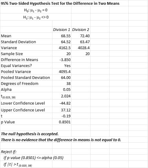
A sales manager for a consumer products company wanted to compare the sales of two sales divisions. When she tested the data for normality, she found the data from both divisions was not normally distributed. The company’s Six Sigma Master Black Belt recommended she use a Mann-Whitney test to determine if there was any statistically significant difference between the two groups. Below is the output of the data she ran. Note, that while there is a mathematical difference between median sales, it is not statistically significant using the Mann-Whitney test.

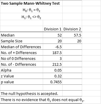
Interestingly, the use of the parametric 2-sample t test results in the same conclusions despite the violation of the assumption of normality. That could be due to the robustness of that assumption.

7 best practices when thinking about non-parametric 

Here are some best practices for using non-parametric methods:

1. Understand the data  

Before applying non-parametric methods, it is important to understand the characteristics of the data. This includes assessing the distribution of the data, identifying outliers, and considering the scale of measurement (nominal, ordinal, or interval).

2. Choose the appropriate test  

There are many different non-parametric tests available, each with different assumptions and requirements. It is important to choose the appropriate test for the research question and data type.

3. Use multiple tests

Using multiple non-parametric tests can provide you with more robust results and help validate findings. However, multiple testing should be done with caution, as it can increase the risk of false positives.

4. Interpret results carefully  

Non-parametric tests often provide p-values and effect sizes that are not directly comparable to those from parametric tests. It is important to carefully interpret the results and consider the limitations of the method.

5. Report results clearly  

When reporting non-parametric results, it is important to clearly state which test was used, how the data was analyzed, and what the results mean in the context of the research question.

6. Consider sample size

 Non-parametric methods can be used with small sample sizes, but as with any statistical analysis, larger sample sizes generally provide more robust results.

7. Use appropriate software  

There are many software packages available for performing non-parametric analysis. It is important to choose a software that is appropriate for the research question and data type, and to ensure that the software is used correctly.

Frequently Asked Questions (FAQ) about non-parametric

What is the difference between parametric and non-parametric methods .

Parametric methods make assumptions about the underlying probability distribution of the data, while non-parametric methods do not. Non-parametric methods are often used when the assumptions of parametric methods are not met. Be aware that parametric tests will often test means while non-parametric tests will use medians.

What are some common non-parametric tests? 

Common non-parametric tests include the Wilcoxon rank-sum test, the Kruskal-Wallis test, and the Mann-Whitney U test.

When should I use non-parametric methods? 

Non-parametric methods should be used when the assumptions of parametric methods are not met, such as when the data is not normally distributed or has outliers.

Are non-parametric methods less powerful than parametric methods?

Non-parametric methods are generally less powerful than parametric methods when the assumptions of parametric methods are met. However, when the assumptions are not met, non-parametric methods can provide more accurate and reliable results.

How do I interpret non-parametric test results?  

Can non-parametric methods be used with small sample sizes .

Yes, non-parametric methods can be used with small sample sizes, but as with any statistical analysis, larger sample sizes generally provide more robust results.

Wrapping up non-parametric

Non-parametric tests allow you to answer statistical questions when your data do not comply with underlying assumptions of the tests. Many statistical tests have assumptions about specific characteristics or underlying distributions of the population data. For example, non-parametric tests are useful when your assumptions call for normality of the data and your data is not normal.

There are non-parametric tests that mirror those of parametric tests. For example, a parametric test for two samples (2-sample t) will have an equivalent non-parametric test (Mann-Whitney). The difference is that the t test will test for the difference in two means while the Mann-Whitney test will test the difference between two medians.

While the parametric tests will have more power for discerning differences, the non-parametric test will be sufficient in most cases. Parametric tests are also quite robust to violations of their assumptions especially when sample sizes are large enough. Non-parametric tests also have some underlying assumptions but they are not related to the population distributions.

About the Author

Ken Feldman

Non-Parametric Test

Non-parametric test is a statistical analysis method that does not assume the population data belongs to some prescribed distribution which is determined by some parameters. Due to this, a non-parametric test is also known as a distribution-free test. These tests are usually based on distributions that have unspecified parameters.

A non-parametric test acts as an alternative to a parametric test for mathematical models where the nature of parameters is flexible. Usually, when the assumptions of parametric tests are violated then non-parametric tests are used. In this article, we will learn more about a non-parametric test, the types, examples, advantages, and disadvantages.

What is Non-Parametric Test in Statistics?

A non-parametric test in statistics does not assume that the data has been taken from a normal distribution . A normal distribution belongs to a parametrized family of probability distributions and includes parameters such as mean, variance, standard deviation, etc. Thus, a non-parametric test does not make assumptions about the probability distribution's parameters.

Non-Parametric Test Definition

A non-parametric test can be defined as a test that is used in statistical analysis when the data under consideration does not belong to a parametrized family of distributions. When the data does not meet the requirements to perform a parametric test, a non-parametric test is used to analyze it.

Reasons to Use Non-Parametric Tests

It is important to access when to apply parametric and non-parametric tests in order to arrive at the correct statistical inference. The reasons to use a non-parametric test are given below:

• When the distribution is skewed, a non-parametric test is used. For skewed distributions, the mean is not the best measure of central tendency, hence, parametric tests cannot be used.
• If the size of the data is too small then validating the distribution of the data becomes difficult. Thus, in such cases, a non-parametric test is used to analyze the data.
• If the data is nominal or ordinal, a non-parametric test is used. This is because a parametric test can only be used for continuous data.

Types of Non-Parametric Tests

Parametric tests are those that assume that the data follows a normal distribution. Examples include ANOVA and t-tests. There are many different methods available to perform a non-parametric test. These tests can also be used in hypothesis testing. Some common non-parametric tests are given as follows:

Mann-Whitney U Test

This non-parametric test is analogous to t-tests for independent samples. To conduct such a test the distribution must contain ordinal data. It is also known as the Wilcoxon rank sum test.

Null Hypothesis: \(H_{0}\): The two populations under consideration must be equal.

Test Statistic: U should be smaller of

\(U_{1} = n_{1}n_{2}+\frac{n_{1}(n_{1}+1)}{2}-R_{1}\) or \(U_{2} = n_{1}n_{2}+\frac{n_{2}(n_{2}+1)}{2}-R_{2}\)

where, \(R_{1}\) is the sum of ranks in group 1 and \(R_{2}\) is the sum of ranks in group 2.

Decision Criteria: Reject the null hypothesis if U < critical value.

Wilcoxon Signed Rank Test

This is the non-parametric test whose counterpart is the parametric paired t-test . It is used to compare two samples that contain ordinal data and are dependent. The Wilcoxon signed rank test assumes that the data comes from a symmetric distribution.

Null Hypothesis: \(H_{0}\): The difference in the median is 0.

Test Statistic: W. W is defined as the smaller of the sums of the negative and positive ranks.

Decision Criteria: Reject the null hypothesis if W < critical value.

This non-parametric test is the parametric counterpart to the paired samples t-test. The sign test is similar to the Wilcoxon sign test.

Test Statistic: The smaller value among the number of positive and negative signs.

Decision Criteria: Reject the null hypothesis if the test statistic < critical value.

Kruskal Wallis Test

The parametric one-way ANOVA test is analogous to the non-parametric Kruskal Wallis test. It is used for comparing more than two groups of data that are independent and ordinal.

Null Hypothesis: \(H_{0}\): m population medians are equal

Test Statistic: H = \(\left ( \frac{12}{N(N+1)}\sum_{1}^{m} \frac{R_{j}^{2}}{n_{j}}\right ) - 3(N+1)\)

where, N = total sample size, \(n_{j}\) and \(R_{j}\) are the sample size and the sum of ranks of the j th group

Decision Criteria: Reject the null hypothesis if H > critical value

Non-Parametric Test Example

The best way to understand how to set up and solve a hypothesis involving a non-parametric test is by taking an example.

Suppose patients are suffering from cancer. They are divided into three groups and different drugs were administered. The platelet count for the patients is given in the table below. It needs to be checked if the population medians are equal. The significance level is 0.05.

As the size of the 3 groups is not same the Kruskal Wallis test is used.

\(H_{0}\): Population medians are same

\(H_{1}\): Population medians are different

\(n_{1}\) = 5, \(n_{2}\) = 3, \(n_{3}\) = 4

N = 5 + 3 + 4 = 12

Now ordering the groups and assigning ranks

\(R_{1}\) = 18.5, \(R_{2}\) = 21, \(R_{3}\) = 38.5,

Substituting these values in the test statistic formula, \(\left ( \frac{12}{N(N+1)}\sum_{1}^{m} \frac{R_{j}^{2}}{n_{j}}\right ) - 3(N+1)\)

H = 6.0778.

Using the critical value table, the critical value will be 5.656.

As H < critical value, the null hypothesis is rejected and it is concluded that there is no significant evidence to show that the population medians are equal.

Difference between Parametric and Non-Parametric Test

Depending upon the type of distribution that the data has been obtained from both, a parametric test and a non-parametric test can be used in hypothesis testing. The table given below outlines the main difference between parametric and non-parametric tests.

Advantages and Disadvantages of Non-Parametric Test

Non-parametric tests are used when the conditions for a parametric test are not satisfied. In some cases when the data does not match the required assumptions but has a large sample size then a parametric test can still be used. Some of the advantages and disadvantages of a non-parametric test are listed as follows:

Advantages of Non-Parametric Test

The advantages of a non-parametric test are listed as follows:

• Knowledge of the population distribution is not required.
• The calculations involved in such a test are shorter.
• A non-parametric test is easy to understand.
• These tests are applicable to all data types.

Disadvantages of Non-Parametric Test

The disadvantages of a non-parametric test are given below:

• They are not as efficient as their parametric counterparts.
• As these are distribution-free tests the level of accuracy is reduced.

Related Articles:

• Summary Statistics
• Probability and Statistics
• T-Distribution

Important Notes on Non-Parametric Test

• A non-parametric test is a statistical test that is performed on data belonging to a distribution whose parameters are unknown.
• It is used on skewed distributions and the measure of central tendency used is the median.
• Kruskal Wallis test, sign test, Wilcoxon signed test and the Mann Whitney u test are some important non-parametric tests used in hypothesis testing.

Examples on Non-Parametric Test

Example 1: A surprise quiz was taken and the scores of 6 students are given as follows:

After giving a month's time to practice, the same quiz was taken again and the following scores were obtained.

Assigning signed ranks to the differences

\(H_{0}\): Median difference is 0. \(H_{1}\): Median difference is positive. W1: Sum of positive ranks = 17.5 W2: Sum of negative ranks = 3.5 As W2 < W1, thus, W2 is the test statistic. Now from the table, the critical value is 2. Since W2 > 2, thus, the null hypothesis cannot be rejected and it can be concluded that there is no difference between the scores of the two tests. Answer: Fail to reject the null hypothesis

\(H_{0}\): Two groups report same number of cases \(H_{1}\): Two groups report different number of cases \(R_{1}\) = 15.5, \(R_{2}\) = 39.5 \(n_{1}\) = \(n_{2}\) = 5 Using the formulas, \(U_{1} = n_{1}n_{2}+\frac{n_{1}(n_{1}+1)}{2}-R_{1}\) and \(U_{2} = n_{1}n_{2}+\frac{n_{2}(n_{2}+1)}{2}-R_{2}\) \(U_{1}\) = 24.5, \(U_{2}\) = 0.5 As \(U_{2}\) < \(U_{1}\), thus, \(U_{2}\) is the test statistic. From the table the critical value is 2 As \(U_{2}\) < 2, the null hypothesis is rejected and it is concluded that there is no evidence to prove that the two groups have the same number of sleepwalking cases. Answer: Null hypothesis is rejected

go to slide go to slide go to slide

Book a Free Trial Class

FAQs on Non-Parametric Test

What is a non-parametric test.

A non-parametric test in statistics is a test that is performed on data belonging to a distribution that has flexible parameters. Thus, they are also known as distribution-free tests.

When Should a Non-Parametric Test be Used?

A non-parametric test should be used under the following conditions.

• The distribution is skewed.
• The size of the distribution is small.
• The data is nominal or ordinal.

What is the Test Statistic Used for the Mann-Whitney U Non-Parametric Test?

The Mann Whitney U non-parametric test is the non parametric version of the sample t-test. The test statistic used for hypothesis testing is U . U should be smaller of \(U_{1} = n_{1}n_{2}+\frac{n_{1}(n_{1}+1)}{2}-R_{1}\) or \(U_{2} = n_{1}n_{2}+\frac{n_{2}(n_{2}+1)}{2}-R_{2}\)

What is the Test Statistic Used for the Kruskal Wallis Non-Parametric Test?

The parametric counterpart of the Kruskal Wallis non parametric test is the one way ANOVA test. The test statistic used is H = \(\left ( \frac{12}{N(N+1)}\sum_{1}^{m} \frac{R_{j}^{2}}{n_{j}}\right ) - 3(N+1)\).

What is the Test Statistic Used for the Sign Non-Parametric Test?

The smaller value among the number of positive and negative signs is the test statistic that is used for the sign non-parametric test.

What is the Difference Between a Parametric and Non-Parametric Test?

A parametric test is conducted on data that is obtained from a parameterized distribution such as a normal distribution. On the other hand, a non-parametric test is conducted on a skewed distribution or when the parameters of the population distribution are not known.

What are the Advantages of a Non-Parametric Test?

A non-parametric test does not rely on the assumed parameters of a distribution and is applicable to all data types. Furthermore, they are easy to understand.

Non-parametric Tests for Psychological Data

• First Online: 28 August 2019

Cite this chapter

• J. P. Verma 2  

2233 Accesses

2 Citations

In most of the psychological studies, data that is generated is non-metric; hence, it is essential to know various non-parametric tests that are available for different situations. Non-parametric tests are used for non-metric data, but if assumptions of the parametric tests are violated, these tests can be used for addressing research questions. Several non-parametric tests are available as a substitute for many parametric tests. For example, chi-square test is an option for correlation coefficient; sign test and median/Mann–Whitney U tests are the options for one-sample t-test and two-sample t-test, respectively; Kruskal–Wallis H test is an option for one-way ANOVA; and Friedman’s test is an option for one-way repeated measures ANOVA. The procedure of these tests has been discussed in this chapter by means of examples. After going through this chapter, one should be able to apply chi-square test, runs test, sign test, median test, Mann–Whitney test, Kruskal–Wallis H test, and Friedman’s test.

This is a preview of subscription content, log in via an institution to check access.

Access this chapter

• Available as PDF
• Read on any device
• Instant download
• Own it forever
• Available as EPUB and PDF
• Durable hardcover edition
• Dispatched in 3 to 5 business days
• Free shipping worldwide - see info

Tax calculation will be finalised at checkout

Purchases are for personal use only

Institutional subscriptions

Similar content being viewed by others

Parametric Tests

Writing about Non-parametric Tests

Author information

Authors and affiliations.

Department of Sport Psychology, Lakshmibai National Institute of Physical Education, Gwalior, India

Prof. J. P. Verma

You can also search for this author in PubMed   Google Scholar

Corresponding author

Correspondence to J. P. Verma .

Rights and permissions

Reprints and permissions

Copyright information

© 2019 Springer Nature Singapore Pte Ltd.

About this chapter

Verma, J.P. (2019). Non-parametric Tests for Psychological Data. In: Statistics and Research Methods in Psychology with Excel. Springer, Singapore. https://doi.org/10.1007/978-981-13-3429-0_12

Download citation

DOI : https://doi.org/10.1007/978-981-13-3429-0_12

Published : 28 August 2019

Publisher Name : Springer, Singapore

Print ISBN : 978-981-13-3428-3

Online ISBN : 978-981-13-3429-0

eBook Packages : Mathematics and Statistics Mathematics and Statistics (R0)

Share this chapter

Anyone you share the following link with will be able to read this content:

Sorry, a shareable link is not currently available for this article.

Provided by the Springer Nature SharedIt content-sharing initiative

• Publish with us

Policies and ethics

• Find a journal
• Track your research

Overview SPSS Nonparametric Tests

Nonparametric Tests - One Sample

Spss z-test for a single proportion.

Z-tests were introduced to SPSS version 27 in 2020.

This tutorial quickly walks you through z-tests for single proportions:

• which options should you select?
• how to interpret the output?
• which assumptions should you meet -and how to test these?
• and way more...

Binomial Test – Simple Tutorial

A binomial test examines if a population percentage is equal to x .

Example: is 45% of all Amsterdam citizens currently single? Or is it a different percentage?

This simple tutorial quickly walks you through the basics.

SPSS Binomial Test Tutorial

This tutorial walks you through running and interpreting a binomial test in SPSS.

With step-by-step example on downloadable practice data file.

SPSS Sign Test for One Median – Simple Example

SPSS sign test for one median the right way. Recode your outcome variable into values higher and lower than the hypothesized median and test if they're distribted 50/50 with a binomial test.

Nonparametric Tests - 2 Independent Samples

Spss z-test for independent proportions tutorial.

This tutorial quickly walks you through z-tests for 2 independent proportions:

SPSS Mann-Whitney Test – Simple Example

The Mann-Whitney test is an alternative for the independent samples t test when the assumptions required by the latter aren't met by the data. The most common scenario is testing a non normally distributed outcome variable in a small sample (say, n < 25).

SPSS Median Test for 2 Independent Medians

SPSS median test evaluates if two groups of respondents have equal population medians on some variable. This easy tutorial quickly walks you through.

Nonparametric Tests - 3(+) Independent Samples

How to run a kruskal-wallis test in spss.

The Kruskal-Wallis test is a nonparametric alternative for a one-way ANOVA .

This tutorial shows when to use it and how to run it in SPSS.

Nonparametric Tests - 2 Related Samples

Spss wilcoxon signed-ranks test – simple example.

SPSS Wilcoxon Signed-Ranks test is used for comparing two metric variables measured on one group of cases. It's the nonparametric alternative for a paired-samples t-test when its assumptions aren't met.

SPSS McNemar Test

SPSS McNemar test is a procedure for testing whether the proportions of two dichotomous variables are equal. The two variables have been measured on the same cases.

SPSS Sign Test for Two Medians – Simple Example

SPSS sign test for two related medians tests if two variables measured in one group of people have equal population medians.

Nonparametric Tests - 3(+) Related Samples

Spss friedman test tutorial.

SPSS Friedman test compares the means of 3 or more variables measured on the same respondents. Like so, it is a nonparametric alternative for a repeated-measures ANOVA that's used when the latter’s assumptions aren't met.

SPSS Cochran Q Test

SPSS Cochran's Q test is a procedure for testing whether the proportions of 3 or more dichotomous variables are equal. These outcome variables have been measured on the same people or other statistical units.

Tell us what you think!

This tutorial has 7 comments:.

By Andy on July 8th, 2020

Please give some public or environmental health related case study for binomial test.

By Ruben Geert van den Berg on July 8th, 2020

What about testing if the percentage of COVID infected people is equal to x ? We're sure you can fill in the details from there, right?

Privacy Overview

• Open access
• Published: 23 May 2024

Interpretation of course conceptual structure and student self-efficacy: an integrated strategy of knowledge graphs with item response modeling

• Zhen-Yu Cao 1 ,
• Feng Lin 2 &
• Chun Feng 3 , 4  

BMC Medical Education volume  24 , Article number:  563 ( 2024 ) Cite this article

111 Accesses

Metrics details

There is a scarcity of studies that quantitatively assess the difficulty and importance of knowledge points (KPs) depending on students’ self-efficacy for learning (SEL). This study aims to validate the practical application of psychological measurement tools in physical therapy education by analyzing student SEL and course conceptual structure.

From the “Therapeutic Exercise” course curriculum, we extracted 100 KPs and administered a difficulty rating questionnaire to 218 students post-final exam. The pipeline of the non-parametric Item Response Theory (IRT) and parametric IRT modeling was employed to estimate student SEL and describe the hierarchy of KPs in terms of item difficulty. Additionally, Gaussian Graphical Models with Non-Convex Penalties were deployed to create a Knowledge Graph (KG) and identify the main components. A visual analytics approach was then proposed to understand the correlation and difficulty level of KPs.

We identified 50 KPs to create the Mokken scale, which exhibited high reliability (Cronbach’s alpha = 0.9675) with no gender bias at the overall or at each item level ( p  > 0.05 ). The three-parameter logistic model (3PLM) demonstrated good fitness with questionnaire data, whose Root Mean Square Error Approximation was < 0.05. Also, item-model fitness unveiled good fitness, as indicated by each item with non-significant p-values for chi-square tests. The Wright map revealed item difficulty relative to SEL levels. SEL estimated by the 3PLM correlated significantly with the high-ability range of average Grade-Point Average ( p  < 0.05 ). The KG backbone structure consisted of 58 KPs, with 29 KPs overlapping with the Mokken scale. Visual analysis of the KG backbone structure revealed that the difficulty level of KPs in the IRT could not replace their position parameters in the KG.

The IRT and KG methods utilized in this study offer distinct perspectives for visualizing hierarchical relationships and correlations among the KPs. Based on real-world teaching empirical data, this study helps to provide a research foundation for updating course contents and customizing learning objectives.

Trial registration

Not applicable.

Peer Review reports

Introduction

Knowledge points (KPs) serve as fundamental units within the realm of learning content, encompassing theories, ideas, thoughts, etc [ 1 ]. Determining the importance and difficulty of KPs is crucial for effective curriculum development [ 2 ]. Experts typically identify key KPs and peripheral KPs aligned with learning objectives [ 3 ]. Key KPs, or important points, are the core concepts of course content. Additionally, KPs can be classified as either complex or simple, considering their respective levels of teaching difficulty. Complex KPs, or difficult points, are challenging for students to master and require more education time [ 4 ]. Apart from teaching proficiency, KPs are considered a relative concept contingent upon student abilities [ 5 ]. Students with advanced abilities may identify certain KPs as relatively easy, while those with weaker abilities might find them comparatively challenging [ 6 ]. As a psychological attribute, the student’s ability is considered a “latent trait”, and is generally an inherent and intricate individual characteristic that cannot be directly measured by instruments or equipment.

In the context of learning theory, latent traits can usually be divided into two types, namely learning capacity and self-efficacy. Learning capacity specifies the capacity that one will produce positive learning outcomes, which can be manifested by the Grade-Point Average (GPA) [ 7 ]. Self-efficacy measured by psychometric questionnaires like the Learning Self-Efficacy Scale for Clinical Skills (L-SES) [ 8 ], reflects the belief in one’s ability to learn effectively [ 9 ].

Recent research has underscored the connection between high self-efficacy for learning (SEL) and successful academic performance [ 9 , 10 , 11 , 12 ]. However, there was still a knowledge gap regarding the varying degrees of difficulty that each student may experience when dealing with specific KPs. The existing tools, like the L-SES with its 12-item scale [ 8 ], primarily assess SEL but do not concurrently measure the difficulty of KPs. This limitation hinders the understanding of students’ learning experiences, as it overlooks the varying degrees of difficulty associated with specific KPs.

To address this gap, this study applied the Item Response Theory (IRT), a theoretical framework for considering person ability, and item difficulty on the same scale (in units of logit). The corresponding test analysis method is item response modeling (IRM), which can quantify how individuals with different levels of the latent trait are likely to respond to specific items. IRT can be broadly categorized into two main types, namely, non-parametric IRT (npIRT) and parametric IRT (pIRT) [ 13 ]. Compared to pIRT with explicit assumptions, the npIRT is more flexible in handling data and makes fewer assumptions about the underlying structure of the item responses. The npIRT may focus on ranking items based on their discriminatory power without assuming specific functional forms. The analytical pipeline for the npIRT and the pIRT modeling has been previously validated [ 14 , 15 , 16 , 17 ] as a sufficient and reliable scaling method [ 18 ], which offers a promising approach to measuring both SEL and the difficulty of KPs.

In addition to investigating the difficulty of KPs in alignment with diverse student abilities, the main purpose of educational activities is to facilitate the construction of knowledge schemas. The construction process of knowledge schemas involves connecting new KPs with existing knowledge [ 19 ]. To effectively assimilate new knowledge, one prerequisite is the acquisition of enough foundational knowledge [ 20 ]. During the dynamic process of expanding and shaping knowledge schemas, certain KPs play a pivotal role by introducing other KPs connected to the overarching schema, which are referred to as necessary points [ 21 ]. Accordingly, KPs should be sorted sequentially to determine the priority of teaching content. The utilization of a knowledge graph (KG) [ 22 ] provides an opportunity for representing KPs as nodes and their relationships as connections. The knowledge graph model (KGM) is the corresponding technical approach to exploring knowledge schemas, enabling the quantitative calculation of the weight of KPs [ 23 ].

This study attempts to offer innovative teaching application methods and explore research directions by incorporating student self-evaluation difficulties of KPs, along with IRT and KGM techniques. Pinpointing the difficult points by the IRT addresses the concern of “which KPs demand additional teaching resources for enhanced comprehension” [ 5 ]. Determining the important points in the KG tackles the query of “which knowledge points are the indispensable core of this course” [ 2 ]. Uncovering the necessary points by the KGM resolves the issue of “which KPs need to be taught first” [ 24 ]. The ultimate goal is to customize teaching plans based on the implication of the difficulty and importance of KPs.

Data collection

This study was approved by the Committee for Ethics in Human Research at the Nanjing University of Chinese Medicine (NJUCM), with the issued number as No. 2021-LL-13(L).

A collaborative process involved a three-person voting method facilitated by three rehabilitation professors. These three rehabilitation professors jointly assessed and selected 100 KPs from the curriculum. Following the completion of the final exam, physical therapy students were engaged in the online questionnaire regarding the difficulty rating of KPs. This survey assessed the perceived difficulty of the 100 KPs based on a five-point Likert scale, where students indicated their perception on a scale ranging from 0 (very easy) to 4 (very difficult).

Statistical tools and methods

The data analysis process, as depicted in Fig.  1 , involved several R packages within the R software (Version 4.2.0) [ 25 ] to facilitate key steps. We used the mokken [ 26 ] and mirt [ 27 ] packages [ 25 ] to construct the IRM and parameter estimation. The ggstatsplot package [ 28 ] was operated for correlation analysis and visualization. The robustbase package [ 29 ] was employed to analyze the upper and lower bounds of skewed distributions. The GGMncv package [ 30 ] was conducted for network modeling, while the backbone package [ 31 ] interpreted the network skeleton structure. The igraph package [ 32 ] was exploited for network visualization and parameter analysis.

Data processing pipeline AISP: automatic item selection procedure; IRT: item response theory; np-IRT: non-parametric IRT; p-IRT: parametric IRT; 1PLM, 2PLM, 3PLM, and 4PLM: logistic item response model with 1 parameter, and 2, 3, and 4 parameters; INFIT: inlier-sensitive fit/information-weighted fit; OUTFIT: outlier-sensitive fit; S-X2: signed chi-squared test statistic; DTF: differential test functioning; DIF: differential item functioning

IRT modelling

Data transformation.

The difficulty rating scores for KPs were binarized from 0-1-2-3-4 to 1-1-1-0-0. Our study employed the “ascending assignment principle” or assigning by confidence. Under this scoring system, 0 indicated students had self-perceived difficulty mastering certain KPs, whereas 1 indicated students were confident that the knowledge point was easy to learn. A higher questionnaire score (total score of all items) corresponded to greater SEL.

To avoid ceiling and floor effects, the mastery ratio (proportion of KPs with a binary value of 1) and the unfamiliarity ratio (proportion of KPs with a binary value of 0) were calculated for each knowledge point. If KPs with a mastery rate or unfamiliarity rate greater than 95%, they are considered pseudo-constant.

Guttman errors were calculated after removing pseudo-constant KPs. The upper fence of the Guttman error distribution was calculated using the corrected box plot [ 29 ]. If Guttman errors exceed the upper fence, it is considered as extreme response bias and would be eliminated. The IRT modeling analysis was conducted as follows. The SEL of students estimated by IRM was defined by the “person ability”, or “θ” value of latent trait. Item difficulty computed by IRM was expressed as the same logit as the person ability. The “outcome” or “learning capacity” implied the academic level measured by exam scores.

Mokken scale analysis

Mokken Scale Analysis (MSA) is a npIRT model, which can extract a parsimonious subset of items from the original questionnaire items. The total score of one or more subsets of items informs the ordering of the latent traits. We adopted the monotone homogeneity model (MHM) as one of Mokken models, which relies on three assumptions to order persons using the sum score on a set of items [ 18 ]: ① Unidimensionality: The scale measures the single latent trait, equivalent to one factor in the scale; ② Local independence: The associations between scores of two items are solely explained by the θ, where the individual item score is conditionally independent given the latent trait; ③ Monotonicity: Monotonicity is depicted as the item characteristic curve (ICC) that increases or remains constant, but cannot decrease as the θ increases. The ICC is plotted to speculate the relation between the θ and the probability of obtaining item scores, which is typically an S-shaped curve.

The homogeneity coefficients, also known as scalability coefficients, are key indicators of MSA. Considering the sample size and number of questionnaire items, the threshold for the global homogeneity coefficient of all items (denoted as H) was set at 0.42 [ 33 ]. According to this boundary value, the automatic item selection procedure (AISP) was exerted to obtain a set of items that meet the unidimensionality [ 34 ]. The inter-item homogeneity coefficient (H ij ) was then calculated, where H ij < 0 violates the MHM assumption.

The conditional association proposed by Straat et al. [ 35 ] was also utilized to compute three W indices to identify the local dependence. The W 1 index detects the positive local dependence (cov(i, j|θ) > 0). The W 2 index determines the likelihood of each item being in a positive local dependence. The W 3 index explores negative local dependence (cov(i, j|θ) < 0). The upper limit of the Tukey threshold regarding each W index distribution is the criteria to screen the extreme W values. If W values are larger than the upper limit, it means the violation of local independence. Additionally, we employed the ICC visualization analysis and counted the number of violations to test for monotonicity in MHM.

Logistic model analysis

Although the MSA can extract a set of items that meets three assumptions of the MHM, it employs face values rather than parameters to characterize person abilities and item difficulties. On the other hand, the stricter pIRT models have been designed to compare individual abilities and item difficulties on the same scale, which also needs to satisfy unidimensionality, local independence, and monotonicity assumptions. Thus, constructing the MHM and extracting candidate items derived from the MSA are more effective in conducting the pIRT modeling [ 15 , 16 , 18 , 35 , 36 , 37 ].

One common unidimensional pIRT model is the logistic item response model. These models implement log odds (Logit) as the unit of measurement for person abilities (θ, i.e., latent traits) and item parameters. Within the logistic model, four key item parameters are illustrated in the fICC [ 38 ]: ① Discrimination (a): This parameter corresponds to the maximum slope value at the inflection point on the ICC. It quantifies how effectively items can differentiate between individuals with high and low abilities. ② Difficulty (b): The θ value corresponds to the inflection point on the ICC. As the b value increases, the ICC shifts to the right, indicating an increase in item difficulties, resulting in a decreased scoring rate for test items, even when person abilities remain unchanged. Conversely, a decrease in the b value shifts the ICC to the left, signifying a decrease in item difficulties. ③ Guessing (g): The lower asymptote of the ICC. If g is greater than zero, it indicates that individuals with low ability have a certain probability of obtaining scores due to guessing. ④ Carelessness (u): The upper asymptote of the ICC. If u is less than 1, it suggests that individuals with high ability may lose points due to carelessness.

These parameters are instrumental in constructing four different logistic models. The 1-parameter logistic model (1PLM) estimates the b value, assuming default values of a = 1 (consistent discrimination for all items), g = 0 (no guessing), and u = 1 (no carelessness). The 2-parameter logistic model (2PLM) estimates a and b, with default values of g = 0 and u = 1. The 3-parameter logistic model (3PLM) estimates a, b, and g, while assuming a default value of u = 1. The 4-parameter logistic model (4PLM) estimates all four parameters. The estimations for the four alternative models are conventionally set in the range of -6 to 6 Logit for θ values, and the parameter estimation usually adopts the expectation-maximization (EM) algorithm. The calculation precision (i.e., EM convergence threshold) default is set as 10 − 5 . The assessment of these models was carried out by two-step tests.

First step assessed the goodness of fit (GOF) of the model and the questionnaire data, including p -value based upon M 2 statistic, root mean square error approximation (RMSEA), Tucker-Lewis index (TLI), and comparative fit index (CFI). This study determines the model fit following the criteria: p  > 0.05 [ 39 ], RMSEA < 0.05 [ 40 ], TLI > 0.95, and CFI > 0.95 [ 41 ].

Second, when multiple models display good fitness, it’s essential to conduct pairwise comparisons using likelihood ratio tests. If the p -value < 0.05 signifies a significant difference between the two models, the model with lower Akaike information criterion (AIC) and Bayesian information criterion (BIC) values is preferred. The p -value is great than 0.05, which indicates no significant difference between the models. Even though the model with a smaller AIC and BIC might be a reasonable choice in this scenario, it’s important to contemplate the inclusion of g and u parameters. A significant positive correlation between total scores and Gutmann errors indicates that individuals with higher scores tend to make more Guttman errors, likely due to carelessness. In this case, including the u parameter is recommended, leaning towards the 4PLM. Conversely, if there’s a significant negative correlation, it suggests that individuals with lower scores are prone to more Guttman errors, possibly resulting from excessive guessing. Here, the g parameter should be integrated, pointing to a preference for the 3PLM.

Analysis of the final model

Four key indicators were employed to evaluate the final model’s internal consistency, including Cronbach’s alpha, Guttman’s lambda-2, Molenaar-Sijtsma statistic, and latent class reliability coefficient (LCRC). As per van der Ark et al. [ 42 ], the LCRC stands out as a superior measure of reliability compared to the other three indicators. A value exceeding 0.9 is deemed indicative of high reliability.

Also, we developed the self-report-based knowledge point learning IRT model. The estimated θ values stand for individuals’ SEL in mastering the course material. The correlation analysis was also performed between the θ values and students’ final exam scores in the “Therapeutic Exercise” course (course learning outcomes), as well as their average GPA (comprehensive learning capacity). The aim was to explore the relationship between SEL and both course learning outcomes and comprehensive learning capacity.

The examination of measurement equivalence, also known as measurement invariance, was conducted to revolve around the principle that individuals with the same θ value exhibit score differences attributable to factors other than θ [ 43 , 44 , 45 ]. These extraneous factor-related differences can be classified into two categories: differential item functioning (DIF) at the item level, and differential test functioning (DTF) at the overall test level. The exclusion of DIF and DTF can ensure unbiased assessment results across different populations by eliminating potential biases introduced by specific items or scales. DIF analysis is built on the concept of anchor items, which are items exhibiting no significant between-group differences in their parameters. The DIF analysis comprises two steps, each step involving an internal iterative process [ 45 ], that is, exploratory DIF analysis and confirmatory DIF analysis.

The initial step involved a stepwise iterative approach, where the assumption of “all other items as anchors (AOAA)” was applied. Each item was sequentially selected to gauge any discernible between-group differences in its parameters (a, b, g, u) using likelihood ratio tests. Any item with a p -value > 0.05 was designated as an anchor item, while items with p- values < 0.05 were categorized as suspected DIF items. These suspected DIF items were methodically removed one by one until every item had undergone inspection. This process yielded two lists: one consisting of anchor items and another comprising suspected DIF items.

The second step was a systematic iterative process, where the assumption of “the suspected DIF item as the anchor item” was derived from the previously identified anchor items. Each item with suspected differential item functioning (DIF) was incorporated into the model one at a time. We then conducted a likelihood ratio test to evaluate any between-group differences in the item parameters. If an item exhibited a p -value < 0.05 and a substantial effect size, it was categorized as a DIF item. Items with p -values < 0.05 but with a small effect size, in accordance with the criteria outlined by Meade [ 44 ], as well as items with p -values exceeding 0.05, were classified as non-DIF items. Upon completing this second-step iteration, the non-DIF items identified during this phase, along with the anchor items from the initial step, were merged to create a conclusive list of non-DIF items. To visualize the results of the second-step analysis, an expected score distribution plot was presented.

In this study, the focus group was the male group, with the female group serving as the reference group. Using the θ values of the focus group as the reference point, we employed the item parameters specific to each group to compute the expected item scores and overall test scores. These calculations enabled the creation of an expected score distribution plot, revealing the comparative performance of both groups.

KG modeling

Data shaping.

The knowledge point rating scores were transformed from 0-1-2-3-4 to 0-0-0-1-1. A dichotomization strategy was employed, assigning a score of 1 to KPs categorized as “difficult” or “very difficult”, and a score of 0 to those deemed “easy”, “relatively easy”, or “slightly difficult”.

Network preparation

Gaussian Graphical Models with Non-Convex Penalties (GGMncv) were used to compute the partial correlation coefficients between KPs [ 30 ]. KPs were considered as network nodes. The partial correlation relationships constituted connections, and the magnitude of the partial correlation coefficients manifested the strength of these connections. This methodology facilitated the construction of a KG rooted in network theory. There was a total of 100 nodes and 1197 connections in our KG. All nodes were interconnected in a singular network structure without any isolated or separate subnetworks.

Skeleton extraction

A three-step process was adopted to extract the skeleton structure of the KG [ 31 ]. The first step extracted a positive signed backbone through the disparity filter method [ 46 ]. The disparity filter determined the significance of the connection values, retaining only those connections that had a significant difference at a significance level of 0.05, with Bonferroni correction for multiple testing. This step led to a 50.7% reduction in connections, transforming the previous network into a signed network, where positive and negative connections were respectively represented as + 1 and − 1.

This yielded a positive signed backbone comprising 104 connections. The positive signed backbone specifically elucidated the positive correlation relationships between KPs, where mastering the knowledge point i aided in comprehending the knowledge point j. 461 negative connections were ruled out due to lack of practical significance, as they meant mastering the knowledge point i would make it more difficult to understand the knowledge point j.

The second step involved network sparsification. The most important connections of each node were extracted from the labeled skeleton with the L-Spar model, as introduced by Satuluri et al. (2011) [ 47 ]. The threshold of the L-Spar model was set to 0, which enabled the preservation of the single most crucial connection for each node. This step led to a further reduction of 2.9% in connections. Finally, a sparse positive signed backbone structure emerged, encapsulating 101 connections.

The third step restored the actual connection values. According to the positive signed backbone structure, the corresponding structure containing the actual connection value was extracted from the original network, thus obtaining the positive backbone of the KG. The positive signed backbone structure only included connections with a value of 1, which resulted in a skeleton structure of the positive correlation relationships in the KG. The positive backbone illustrates the most important positive correlation relationship structure in the KG, which could be further utilized to examine the weight of each knowledge point.

Network analysis

The term “ego” denoted a specific knowledge point that was selected for examining its weight. ① Degree (DEG) and weighted degree (wDEG): DEG measures the number of connections a given ego node has, while wDEG considers the cumulative strength or weight value of those connections. A higher value indicates that the ego has a greater local impact on the network. ② Betweenness (BET): BET of the ego quantifies the information flow. The range of values is standardized to 0–1. A higher value indicates that the ego serves as a bottleneck, meaning other nodes rely on it to connect. ③ Hub score (HUB): HUB exhibits the centrality of the ego as an information hub within the network. It considers not only the number and strength of connections held by the ego but also the connections of the ego’s neighboring nodes. The range of values is standardized to 0–1, with a higher value signifying a more central position for the ego in the network. ④ Laplacian centrality (LAP): LAP measures the extent of disruption to the overall network structure if the ego is removed. The extent of damage will involve the overall network connectivity and structure if the ego is removed. A higher value indicates that the ego is more indispensable to the network.

Demographic

218 students (62 male and 156 female) majoring in Rehabilitation Therapy at the NJUCM were enrolled in this study. 10 excluded students took ≤ 100s to complete the questionnaire, and were therefore excluded from this study, as their responses were considered too hasty. The results of the remaining 208 students (56 males and 152 females) were specified for further analysis. The average time to complete the questionnaire was 205.00 s (s) [95% CI: 106.35s, 660.32s]. When stratified by gender, female and male students completed the questionnaire in 212.50s [95% CI: 110.65s, 680.87s] and 189.50s [95% CI: 104.88s, 455.00s] respectively, with no significant gender differences (Kruskal-Wallis χ 2  = 3.585, df = 1, p  = 0.0583, η 2  = 0.0173). Average final exam scores were 86.00 [95% CI: 63.00, 95.00] for females, and 82.00 [95% CI: 62.38, 95.88] for males, without significant gender differences (Kruskal -Wallis χ 2  = 3.4216, df = 1, p  = 0.0644, η 2  = 0.0165). The final exam GPA was 3.35 [95% CI: 2.43, 3.98], of which 3.42 [95% CI: 2.46, 3.97] GPA for females and 3.20 [95% CI: 2.41, 4.00] GPA for males. Although there was a significant difference in GPA across gender (Kruskal-Wallis χ 2  = 9.4402, df = 1, p  = 0.0021), the effect was small ( η 2  = 0.0456) and considered negligible.

IRT modeling results

Data preparation.

The difficulty rating of 100 KPs was binarized, which did not exhibit constant values. All of them entered the following IRM. There were no pseudo-constant KPs after dichotomization. As also shown in Figure S1 , no students were excluded due to exceeding the criterion of the upper limit of Guttman errors, thereby allowing integration of the data collected from 208 students into the subsequent IRM phase.

Non-parametric IRT: mokken scale analysis

Aisp analysis (table s1 ).

The threshold of 0.42 was set for the H, which led to the removal of 33 items that did not align with any specific dimension. There were 67 remaining items divided into 5 dimensions (scales), of which 50 items were in dimension 1. Elevating the H threshold did not increase in the number of items allocated to any dimension. Following the methodology recommended by Straat et al. [ 33 ], this study adopted the H threshold of 0.42. Consequently, 50 items from dimension 1 (scale 1) were chosen for further detailed analysis (Table S2 ).

Unidimensionality analysis

The 50-item scale exhibited an H of 0.4756 and a standard error (SE) of 0.0355. In accordance with the criteria established by Sijtsma and van der Ark [ 26 ], the homogeneity of our scale was determined to be at a medium level. Given that the extracted items were situated within dimension 1, there was no need for additional assessments of unidimensionality.

Local independence analysis

According to Sijtsma and van der Ark [ 26 ], if the relationship between any two items i and j violates the local independence given H ij < 0, the MHM was not satisfied. The minimum value of H ij for the 50-item scale was 0.2063, confirming that none of the H ij values violated the prerequisites of the MHM. Moreover, the W 2 index also affirmed the absence of any items engaged in locally positive dependent relationships [ 35 ].

Monotonicity analysis

In the monotonicity test, if the diagnostic critical value (Crit) is ≥ 80, it can be considered a significant violation [ 48 ]. There were no obvious violations in 50 KPs (Table S3), which conformed to monotonicity. The monotonicity can also be further confirmed by the ICC shape of the model built in the pIRT stage. The monotonicity was achieved when the ICC of each item increased with θ but did not decrease (Figure S2).

Parameter IRT: logistic regression model analysis

Model-data fit analysis.

As shown in Table S4, the p values resulted from the M 2 test for all models yielding a value of 0, but the RMSEA of the 3PLM fell below 0.05. The TLI and CFI for all models exceeded 0.95. Therefore, all models were assigned for pairwise comparisons.

Model-model fit comparison

In Table S5, a significant difference (χ 2 (49)  = 77.2966, p  = 0.0061) was observed between the 1PLM and 2PLM (χ 2 (49)  = 77.2966, p  = 0.0061), with 1PLM exhibiting a lower BIC (ΔBIC = -184.2427), suggesting potential superiority to 2PLM. However, there was no significant difference when comparing the 1PLM to either the 3PLM (χ 2 (99)  = 88.6090, p  = 0.7637), or the 4PLM (χ 2 (149)  = 121.8965, p  = 0.9492).

As illustrated in Figure S3, the total scores of the 50-item scale for each student were negatively correlated with the number of Guttman errors ( p  = 1.51 × 10 − 22 ). The correlation coefficient ( \( {\widehat{\rho }}_{Spearman}\) = -0.61) fell within the range of 0.4–0.7, indicating a moderate correlation according to Akoglu’s standards [ 49 ]. This correlation revealed that students with lower scores tended to demonstrate more Guttman errors, implying that they were more likely to guess correctly on items with higher difficulty. This observation underscored the importance of considering guessing behavior in the analysis. Additionally, there was no significant positive correlation, suggesting higher-scoring students did not have more Guttman errors, i.e., they did not lose scores on items with lower difficulty, and thus, the carelessness parameter did not need to be considered.

The 3PLM was ultimately chosen, which did not have a significant difference with 1PLM and additionally incorporated a guessing parameter compared to the 1PLM. Guessing was the lower bound of the ICC, as shown in Figure S2, where a number of KPs (such as kp.75, kp.55, kp.31, and kp.14) had non-zero guessing values. To ensure the property of the 3PLM result, considering the small sample size, we also performed Monte Carlo simulation that generated 500 models with each simulating 1000 response patterns [ 50 ].

Reliability analysis

Cronbach’s α = 0.9684, Guttman’s λ2 = 0.9689, Molenaar Sijtsma Statistic = 0.9708, LCRC = 0.9776. All four coefficients were > 0.95, indicating good internal consistency for the 50-item scale.

Grade-related analysis

As shown in Fig.  2 , the estimated SEL was not significantly correlated with exam scores ( p  = 0.81) or GPA ( p  = 0.81). However, within the range of θ > 0, a weak positive correlation was observed between GPA and θ ( p  = 0.02, r  = 0.22).

Correlation of exam or GPA scores with full range, < 0, or > 0 values of θ

Gender bias analysis

The distribution of expected item scores (Figure S4) and expected test scores (Figure S5) suggested that the 50-item scale did not elucidate significant gender bias.

Model parameter analysis

Table  1 displayed the three parameters of the 3PLM arranged in descending order of difficulty. The majority of items illustrated a guessing parameter of either 0 or very close to zero (< 0.1). The item with the highest guessing parameter was kp.31 (g = 0.2803).

Table  1 also displayed the model fit test results for each item. Only kp.14 showed significant differences in the S-X 2 test ( p  = 0.0466), but its RMSEA (0.0575) reached a publishable level, as suggested by Xia and Yang [ 41 ]. Furthermore, the OUTFIT (1.0073) and INFIT (0.9765) for kp.14 both fell within the recommended range of 0.7 to 1.3 according to the thumb rule for item fit [ 51 ]. The z-OUTFIT (0.1431) and z-INFIT (-0.131) also fell within the acceptable range of z values (-2.0 to 2.0). Therefore, we concluded that kp.14 fit well in the model.

Total score conversion

There was a significant positive correlation between the total score (TTS) on the 50-item scale and the model-estimated θ value ( p  = 1.96 × 10 − 235 , \( {\widehat{\rho }}_{Spearman}\) = 1.0) (Figure S6). The binomial function to facilitate conversion between these two variables can be applied as follows: \( \widehat{\theta }= - 2.09+0.0322\times TTS+0.000622\times TT{S}^{2}\) .

Wright map analysis

Figure  3 showed the student W.,T.’s SEL (-0.4165 Logit). For the student W.,T., the items with the lowest difficulty within his learning competency area were identified as kp.14 (Muscular endurance) and kp.78 (Different balance forms). The student W.,T. should prioritize to grasp these KPs.

Wright map denoting self-efficacy of student W.,T. The * symbol indicated W.,T received 0 on items in the difficulty rating questionnaire after binarization, which are the items the student perceived as difficult. Knowledge points below the ability line are relatively easy to master, while those above the ability line are relatively difficult. Therefore, the area below the ability line represents competency, while the area above represents challenging points

Knowledge graph analysis

Network parameters for knowledge points.

We investigated a KGM composed of 100 KPs, revealing a backbone structure with 68 connections. The connection values were indicated by partial correlation coefficients, ranging from a minimum of 0.106 (weak correlation) to a maximum of 0.464 (moderate correlation) [ 49 ].

The analysis of network parameters of KPs within the backbone structure (Table S6) identified 39 isolated points with a degree of 0. The top three KPs in terms of hub score were kp.46 (1.00, Indications for joint mobility techniques), kp.13 (0.8480, Muscle strength), and kp.90 (0.8204, Contraindications for PNF technique). These three points also held the top three in terms of the BET.

The top three KPs considering Laplacian centrality were kp.46 (Indications for joint mobility techniques), kp.13 (Muscle strength), and kp.63 (Indications for joint mobilization). These three KPs also ranked among the top three in terms of weighted degrees. Overall, kp.46 not only featured prominently in the IRM, but also occupied the most critical position within the backbone structure, underscoring its significance in the knowledge structure of the course “Therapeutic Exercise”. According to Table  1 , kp.46 had a relatively low difficulty (-0.8479), which fell below the mean difficulty of 50 items (-0.6346). Moreover, it exhibited moderate discrimination (2.5353), closely aligning with the mean discrimination of 50 items (2.42046).

Visualization of the main component in the backbone structure

The primary subnetwork within the backbone structure, identified as the main component, comprised 58 nodes, with 29 KPs incorporated into the final IRM. This main component captured 66 out of the 68 connections in the backbone structure. Figure  4 showed the visualization of this main component. The layout was improved by adopting the Sugiyama method for unveiling its hierarchical structure [ 52 , 53 ].

Main component in backbone structure of knowledge graph for Physical Therapy The knowledge points in IRT model (red) were tagged with discrimination parameter

Adapting teaching strategies stemming from the difficulty of KPs is essential for ensuring quality management in curriculum development. However, there is a lack of current reports that quantitatively assess the self-perceived learning difficulty of KPs in medical education. Course difficulty can be categorized into teaching difficulty and learning difficulty from the perspectives of teachers and students, respectively. To effectively evaluate the learning difficulty of KPs, it is necessary to consider students’ learning capacities.

Clinical education applies a wide range of assessment formats, and structured exams are not consistently employed. This diversity poses a substantial challenge when weighing the difficulty of KPs. Meanwhile, the difficulty of KPs can be intertwined with students’ personal traits. Consequently, integrating comprehensive methods to discern students’ personal traits, evaluate the difficulty of KPs, and understand the correlations between different KPs, is a critical process in achieving pedagogical excellence.

The study extracted 100 KPs from the course “Therapeutic Exercise” to investigate students’ perceived difficulty in comprehending KPs. The npIRT and pIRT modeling were sequentially conducted to obtain a parsimonious item set that could be sufficient to distinguish the personal trait levels of the participants without gender bias. IRM was employed to estimate students’ SEL and item difficulty. Students’ SEL was referred to person ability or θ in the IRM. It should be noted that the interpretation of item difficulties is determined by the binarization strategy, indicating the difficulty of attaining scores. In this study, we assigned value 1 as self-confidence in the questionnaire. Therefore, the practical meaning of item difficulty was the difficulty of being self-confident about mastering certain KPs.

Furthermore, graph modeling techniques were also applied to construct a KG based on the conditional association of difficulty correlations among each knowledge point. Although the KG established in this research might not exactly mirror the knowledge schema formed by students through course learning, it can be used to analyze the knowledge schema affected by personal traits. In other words, it can be regarded as the correlation structure of KPs’ difficulty under the influence of SEL.

Implication of the IRM-derived student ability

Our result did not find a significant correlation between one-time exam scores and θ values. However, a significant correlation between the GAP and the estimated θ values, particularly within the spectrum of positive θ values. This correlation supports the reliability of the model which contains 50 KPs, in evaluating students’ learning abilities.

Our findings are in line with the research conducted by Richardson et al. [ 7 ]. They propose that GPA cannot be solely explained by exam scores, for example, the Scholastic Aptitude Test. They indicate that exam scores are a one-time assessment of course-specific learning effectiveness, while GPA can reveal broader academic performance. GPA is a comprehensive indicator of students’ academic performance, reflecting not only learning abilities but also potential career prospects. They conducted correlation analyses involving GPA during undergraduate university with various traits of students. Their research unveiled a medium-to-large correlation between students’ SEL and GPA, with academic self-efficacy (ASE) exhibiting a medium correlation and performance self-efficacy (PSE) showing a strong correlation. Among the 50 factors they examined, PSE showed the strongest correlation with GPA.

Self-efficacy was first introduced by Bandura to manifest individuals feeling of confidence in their capabilities necessary to reach specific goals [ 9 ]. Richardson further defines the self-efficacy into the ASE and PSE. ASE means students’ general perception of their academic competence, which is specifically described as “I have a great deal of control over my academic performance in my courses”. PSE encompasses students’ perceptions of their academic performance capability, as articulated by “What is the highest GPA that you feel completely certain you can attain”. ASE predominantly focuses on self-ability level, while PSE is oriented towards evaluating the anticipated outcomes of the learning process. Our study adopted the difficulty of the KPs scale that was analogous to the concept of PSE as described by Richardson et al. [ 7 ], as both aim to gauge the extent of knowledge mastery with complete certainty.

The results of the correlational analysis within this study suggested that SEL, derived from a questionnaire on KPs’ difficulty, can be categorized into two distinct types: positive SEL and negative SEL. For students displaying positive SEL, there was a weak positive correlation between GPA and SEL ( p  = 0.02, r  = 0.22). It indicated that higher SEL corresponded to higher GPAs, which aligns with self-efficacy theory [ 9 ].

On the contrary, this study also identified negative SEL that failed to predict the one-time course exam scores or correlate the comprehensive learning ability measured by GPA. Therefore, it further suggests that SEL based on psychological questionnaires and learning outcomes based on exams should be treated differently. When evaluating students’ learning abilities, reliance on one-time assessment results alone is insufficient.

Furthermore, how to foster positive SEL in students to enhance their overall learning capabilities is also crucial. Encouraging individuals to set realistic and attainable goals can build confidence and contribute to a positive self-perception [ 54 ]. The following might offer a practical example to assist students in establishing personal goals regarding their person ability as well as importance and difficulty of KPs.

Practical example based on the wright map and the knowledge graph

The wright map displays both persons (in terms of their ability) and items (in terms of their difficulty) on the same scale. It was plotted according to individual θ values to assess individual competency, delineating areas of competence (below the θ value) and incompetence (above the θ value). The analysis of a student’s θ was instrumental in pinpointing specific KPs that warrant focused review. Table  1 , as provided by 3PLM, offered insights to educators to identify KPs demanding increased attention during future teaching endeavors. KPs characterized by higher difficulty should be allocated more teaching time and resources. Furthermore, KPs with higher discrimination, exemplified by kp.31 (motor unit, with the highest discrimination), in this example, should be subjected to more in-class assessments and feedback. Proficiency in these highly discriminative KPs plays a pivotal role in refining the individual ability.

We selected 100 KPs that were considered important points, while 50-item 3PLM could distinguish the difficulty levels of KPs, so as to figure out the relative difficult points. The excluded items were also important for the course, but they were not “simplified enough to distinguish student abilities in IRT model”. Since the items aside from the model did not have difficulty parameters, how to assess the difficulty of these items was another puzzle that needed to be addressed.

In order to solve the above issue, this study also applied the Gaussian random graph model leveraging conditional correlations to calculate partial correlations between different KPs. The correlation between two KPs within the graph model displayed their “difficulty correlation”. In other words, how likely it was that when one knowledge point was difficult or very difficult, the other knowledge point exhibited a similar difficulty level. Therefore, the KG portrayed the relationships based on difficulty correlations.

An examination of the skeleton structure of the KG, as depicted in Fig.  4 , revealed that kp.63 (indications for joint mobilization) occupied the highest position within the hierarchical structure. Notably, it was observed that KPs capable of distinguishing individual traits did not necessarily hold prominent positions within the network. Regarding the principle of constructing graph models based on risk correlation relationships, if important positions are not thoroughly mastered, it would increase the risk of not comprehending other associated items. Therefore, the item kp.46, as a necessary point, which occupied a crucial position and had a certain level of discrimination, should be prioritized for the student to master.

Limitations and future directions

This study was not without its limitations, which were rooted in the constraints imposed by real-world teaching conditions. These limitations provide opportunities for further improvement.

Firstly, the sample size in our study remained relatively small, and the research was confined to specific courses and KPs. We also observed from the Wright map that a majority of KPs within a similar difficulty range, posing a challenge in distinguishing between individuals with high and low abilities. To enhance the robustness of the findings, we would progressively increase the sample size in each cohort of students in future research. There is also a need to continuously broaden the curriculum by incorporating new KPs and domains, extending the generalizability of our findings. Integrating E-learning platforms with the capability to customize and adapt teaching plans through expert-selected, student-rated questionnaires assessing the difficulty of KPs, holds promise for enhancing the educational experience.

Secondly, our study relied on cross-sectional data, and the difficulty questionnaire was administered only once. While GPAs provide a more comprehensive manifestation of the PSE compared to one-time exams, there is still a requirement for quantitative evidence to support long-term effect of SEL on academic performance. Thus, a promising avenue for future research involves undertaking longitudinal studies to explore the impact of adjusted SEL on long-term academic performance. Our approach could potentially provide a measurement tool for assessing the effectiveness of different interventions aimed at improving SEL over an extended period in future studies.

Thirdly, the validity indicators of the model were singular. Future research should consider supplementing exam scores with other learning ability assessment scales, as well as novel measures like brain-computer interfaces and online learning behavior records. These additions will provide valuable multimodal data to evaluate knowledge point significance and candidate abilities more comprehensively. Despite these limitations, this study introduced an innovative and up-to-date quantitative analysis approach, and its results serve as a foundation for ongoing improvement.

Fourthly, the KGM in this study involved a narrow concept network model which requires to integration of various elements of multiple types such as courses, personnel, and locations, as well as multiple relationship structures. This will enable the incorporation of person abilities and item difficulties calculated by the IRM as indicators for related elements, resulting in a more holistic KG for a comprehensive evaluation of the teaching process [ 23 ].

Lastly, the questionnaire was based on students’ self-assessment of the difficulty of KPs, which could reflect the students’ SEL as θ values. Although the IRM defines the θ as personal ability, it might not be directly equated to students’ learning abilities. Nevertheless, the correlation between SEL and GPA provided partial evidence that the questionnaire could also be a useful tool for evaluating learning abilities. Research into the relationships between psychological traits and learning ability traits could become a promising long-term avenue for investigation, and this study contributes practical evidence and tools to this evolving field.

This study employs a self-assessment questionnaire to achieve students’ perceptions of the difficulty of KPs. It integrates the IRM and KGM to quantitatively assess parameters like students’ SEL, the difficulty level of being self-confident about mastering certain KPs, and importance of KPs. The results affirm that IRM and KGM offer quantitative metrics rooted in empirical data. These metrics are instrumental in identifying and categorizing important, difficult, and necessary points within the curriculum. Furthermore, our study serves as a valuable tool for establishing an evidence-based and refined teaching management approach, thereby enhancing the overall quality of education.

Data availability

The datasets used and/or analyzed during the current study are available from the corresponding author on reasonable request.

Bossé É, Barès M. Knowledge and its dimensions. In: Barès M, Bossé É, editors. Relational Calculus for actionable knowledge. Cham: Springer International Publishing; 2022. pp. 45–115.

Chapter   Google Scholar  

Whetten DA. Principles of effective Course Design: what I wish I had known about learning-centered teaching 30 years ago. J Manag Educ. 2007;31:339–57.

Article   Google Scholar  

Li W, Li X, Wu W. Knowledge Innovation mechanism based on linkages between Core Knowledge and Periphery Knowledge: the Case of R&D Cooperation between latecomers and forerunners. Complexity. 2022;2022:e8417784.

Google Scholar  

Shou Z, Lai J-L, Wen H, Liu J-H, Zhang H. Difficulty-based Knowledge Point Clustering Algorithm using students’ multi-interactive behaviors in Online Learning. Math Probl Eng. 2022;2022:e9648534.

Guo H, Yu X, Wang X, Guo L, Xu L, Lu R. Discovering knowledge-point importance from the learning-evaluation data. Int J Distance Educ Technol. 2022;20:1–20.

Chen SY, Wang J-H. Individual Differences and Personalized Learning: a Review and Appraisal. Univers Access Inf Soc. 2021;20:833–49.

Richardson M, Abraham C, Bond R. Psychological correlates of university students’ academic performance: a systematic review and meta-analysis. Psychol Bull. 2012;138:353–87.

Kang Y-N, Chang C-H, Kao C-C, Chen C-Y, Wu C-C. Development of a short and universal learning self-efficacy scale for clinical skills. PLoS ONE. 2019;14:e0209155.

Bandura A. Self-efficacy: toward a unifying theory of behavioral change. Psychol Rev. 1977;84:191–215.

Collard A, Gelaes S, Vanbelle S, Bredart S, Defraigne J-O, Boniver J, et al. Reasoning versus knowledge retention and ascertainment throughout a problem-based learning curriculum. Med Educ. 2009;43:854–65.

Honicke T, Broadbent J, Fuller-Tyszkiewicz M. The self-efficacy and academic performance reciprocal relationship: the influence of Task Difficulty and Baseline Achievement on Learner Trajectory. High Educ Res Dev. 2023;42:1936–53.

Honicke T, Broadbent J. The influence of academic self-efficacy on academic performance: a systematic review. Educ Res Rev. 2016;17:63–84.

Sijtsma K, Meijer RR. 22 nonparametric item response theory and special topics. In: Rao CR, Sinharay S, editors. Handbook of statistics. Elsevier; 2006. pp. 719–46.

Feng C, Jiang Z-L, Sun M-X, Lin F. Simplified post-stroke Functioning Assessment based on ICF via Dichotomous Mokken Scale Analysis and Rasch Modeling. Front Neurol. 2022;13:827247.

Jiang Y-E, Zhang D-M, Jiang Z-L, Tao X-J, Dai M-J, Lin F. ICF-Based simple scale for children with cerebral palsy: application of Mokken scale analysis and Rasch modeling. Dev Neurorehabilitation. 2023;:1–18.

Feng C, Geng B-F, Liu S-G, Jiang Z-L, Lin F. Activity and participation in haemophiliacs: item response modelling based on international classification of functioning, disability and health. Haemophilia. 2022. https://doi.org/10.1111/hae.14702 .

CHEN J-J, ZHU Z-Y, BIAN J-J, LIN F. Nutrition-associated health levels in persons with cancer: item response modelling based on the International Classification of Functioning, disability and health. Eur J Phys Rehabil Med. 2023;59:593–604.

Stochl J, Jones PB, Croudace TJ. Mokken scale analysis of mental health and well-being questionnaire item responses: a non-parametric IRT method in empirical research for applied health researchers. BMC Med Res Methodol. 2012;12:74.

van Kesteren MTR, Meeter M. How to optimize knowledge construction in the brain. Npj Sci Learn. 2020;5:1–7.

Brod G. Toward an understanding of when prior knowledge helps or hinders learning. Npj Sci Learn. 2021;6:1–3.

Leake DB, Maguitman AG, Reichherzer T. Understanding Knowledge Models: Modeling Assessment of Concept Importance in Concept Maps. 2004.

Chaudhri VK, Baru C, Chittar N, Dong XL, Genesereth M, Hendler J, et al. Knowledge graphs: introduction, history, and perspectives. AI Mag. 2022;43:17–29.

Aliyu I, Department of Computer Science ABUZ, Aliyu DKAF, Department of Computer Science ABUZ. Development of Knowledge Graph for University Courses Management. Int J Educ Manag Eng. 2020;10:1.

Moro C, Douglas T, Phillips R, Towstoless M, Hayes A, Hryciw DH, et al. Unpacking and validating the integration core concept of physiology by an Australian team. Adv Physiol Educ. 2023;47:436–42.

R Core Team. A language and environment for statistical computing. 2022.

Sijtsma K, van der Ark LA. A tutorial on how to do a Mokken Scale Analysis on your test and Questionnaire Data. Br J Math Stat Psychol. 2017;70:137–58.

Chalmers RP. Mirt: a Multidimensional Item Response Theory Package for the R environment. J Stat Softw. 2012;48:1–29.

Patil I. Visualizations with statistical details: the ggstatsplot approach. J Open Source Softw. 2021;6:3167.

Hubert M, Vandervieren E. An adjusted boxplot for skewed distributions. Comput Stat Data Anal. 2008;52:5186–201.

Williams DR. Beyond Lasso: A Survey of Nonconvex Regularization in Gaussian Graphical Model. 2020.

Neal ZP. Backbone: an R package to extract network backbones. PLoS ONE. 2022;17:e0269137.

Csardi G, Nepusz T. The igraph software package for complex network research. Interjournal Complex Syst. 2006;1695.

Straat JH, van der Ark LA, Sijtsma K. Minimum sample size requirements for Mokken Scale Analysis. Educ Psychol Meas. 2014;74:809–22.

Straat JH, van der Ark LA, Sijtsma K. Comparing optimization algorithms for Item Selection in Mokken Scale Analysis. J Classif. 2013;30:75–99.

Straat JH, van der Ark LA, Sijtsma K. Using Conditional Association To Identify Locally Independent Item Sets. Methodology. 2016;12:117–23.

Feng C, Lai Q-L, Ferland A, Lin F. Mandarin Stroke Social Network Scale and Item Response Theory. Front Stroke. 2022;1.

Koopman L, Zijlstra BJH, van der Ark LA. A two-step, test-guided mokken scale analysis, for nonclustered and clustered data. Qual Life Res. 2021. https://doi.org/10.1007/s11136-021-02840-2 .

Brzezińska J. Item response theory models in the measurement theory. Commun Stat - Simul Comput. 2020;49:3299–313.

Xu J, Paek I, Xia Y. Investigating the behaviors of M2 and RMSEA2 in fitting a Unidimensional Model to Multidimensional Data. Appl Psychol Meas. 2017;41:632–44.

Maydeu-Olivares A, Joe H. Assessing approximate fit in categorical data analysis. Multivar Behav Res. 2014;49:305–28.

Xia Y, Yang Y, RMSEA, CFI. Structural equation modeling with ordered categorical data: the Story they tell depends on the estimation methods. Behav Res Methods. 2019;51:409–28.

van der Ark LA, van der Palm DW, Sijtsma K. A latent Class Approach to estimating test-score reliability. Appl Psychol Meas. 2011;35:380–92.

Liu X, Jane Rogers H. Treatments of Differential Item Functioning: a comparison of four methods. Educ Psychol Meas. 2022;82:225–53.

Meade AW. A taxonomy of effect size measures for the differential functioning of items and scales. J Appl Psychol. 2010;95:728–43.

Nugent WR, Understanding DIF. Description, methods, and Implications for Social Work Research. J Soc Soc Work Res. 2017;8:305–34.

Serrano MA, Boguñá M, Vespignani A. Extracting the multiscale backbone of complex weighted networks. Proc Natl Acad Sci U S A. 2009;106:6483–8.

Satuluri V, Parthasarathy S, Ruan Y. Local graph sparsification for scalable clustering. In: Proceedings of the 2011 ACM SIGMOD International Conference on Management of data (SIGMOD'11). New York, NY, USA: Association for Computing Machinery;2011. pp. 721–732. https://doi.org/10.1145/1989323.1989399 .

van der Ark LA. New Developments in Mokken Scale Analysis in R. J Stat Softw. 2012;48:1–27.

Akoglu H. User’s guide to correlation coefficients. Turk J Emerg Med. 2018;18:91–3.

Harwell M, Stone CA, Hsu T-C, Kirisci L. Monte Carlo Studies in Item Response Theory. Appl Psychol Meas. 1996;20:101–25.

Hodge KJ, Morgan GB. Stability of INFIT and OUTFIT compared to simulated estimates in Applied setting. J Appl Meas. 2017;18:383–92.

Nikolov NS. Sugiyama Algorithm. In: Kao M-Y, editor. Encyclopedia of algorithms. New York, NY: Springer; 2016. pp. 2162–6.

Sugiyama K, Tagawa S, Toda M. Methods for Visual understanding of Hierarchical System structures. IEEE Trans Syst Man Cybern. 1981;11:109–25.

Bandura A. Self-efficacy: the exercise of control. New York, NY, US: W H Freeman/Times Books/ Henry Holt & Co; 1997.

Download references

Acknowledgements

We extend our gratitude to Amanda Ferland for her meticulous proofreading, addressing grammar errors, and refining the expression of our work.

This study was supported by the following teaching fundings.

(1) National Higher Education of Traditional Chinese Medicine “14th Five-Year Plan” 2023 Educational Research Project (YB-23-21): Research on the Reform of Fine Teaching Management of Traditional Chinese Medicine Colleges and Universities Driven by Digital Educational Measurement Technology - Taking the Therapeutic Exercise Course as an Example. (2) 2021 Jiangsu Province Higher Education Teaching Reform Research Project(2021JSJG295): Exploration of the Teaching Content System of Rehabilitation Therapy with Chinese Medicine Characteristics Based on the Standard of International Classification of Functioning, Disability and Health (ICF). (3) Shanghai Rising-Star Program & Shanghai Sailing Program (23YF1433700).

Author information

Authors and affiliations.

Department of Rehabilitation Medicine, School of Acupuncture-Moxibustion and Tuina, School of Health Preservation and Rehabilitation, Nanjing University of Chinese Medicine, 210023, Nanjing, China

Zhen-Yu Cao

School of Rehabilitation Medicine, Nanjing Medical University, 211100, Nanjing, China

School of Medicine, Tongji University, 200331, Shanghai, China

The Center of Rehabilitation Therapy, The First Rehabilitation Hospital of Shanghai, Rehabilitation Hospital Affiliated to Tongji University, 200090, Shanghai, China

You can also search for this author in PubMed   Google Scholar

Contributions

FL, ZY.C, and CF contributed to the research concept, supervised the entire study; ZY.C collected data. FL performed the analysis, generated the images, and wrote the manuscript with ZY.C and CF; All authors contributed to the article and approved the submitted version.

Corresponding author

Correspondence to Chun Feng .

Ethics declarations

Ethics approval and consent to participate.

This study was approved by the Institutional Ethics Committee of Nanjing University of Chinese Medicine (No. NJUCM 2021-LL-13(L)). The research was conducted ethically, with all study procedures being performed in accordance with the requirements of the World Medical Association’s Declaration of Helsinki. Written informed consent was obtained from each participant/patient for study participation and data publication.

Conflict of interest

The authors declare no conflict of interest.

Additional information

Publisher’s note.

Springer Nature remains neutral with regard to jurisdictional claims in published maps and institutional affiliations.

Electronic supplementary material

Below is the link to the electronic supplementary material.

Supplementary Material 1

Rights and permissions.

Open Access This article is licensed under a Creative Commons Attribution 4.0 International License, which permits use, sharing, adaptation, distribution and reproduction in any medium or format, as long as you give appropriate credit to the original author(s) and the source, provide a link to the Creative Commons licence, and indicate if changes were made. The images or other third party material in this article are included in the article’s Creative Commons licence, unless indicated otherwise in a credit line to the material. If material is not included in the article’s Creative Commons licence and your intended use is not permitted by statutory regulation or exceeds the permitted use, you will need to obtain permission directly from the copyright holder. To view a copy of this licence, visit http://creativecommons.org/licenses/by/4.0/ . The Creative Commons Public Domain Dedication waiver ( http://creativecommons.org/publicdomain/zero/1.0/ ) applies to the data made available in this article, unless otherwise stated in a credit line to the data.

Reprints and permissions

About this article

Cite this article.

Cao, ZY., Lin, F. & Feng, C. Interpretation of course conceptual structure and student self-efficacy: an integrated strategy of knowledge graphs with item response modeling. BMC Med Educ 24 , 563 (2024). https://doi.org/10.1186/s12909-024-05401-6

Download citation

Received : 22 November 2023

Accepted : 08 April 2024

Published : 23 May 2024

DOI : https://doi.org/10.1186/s12909-024-05401-6

Share this article

Anyone you share the following link with will be able to read this content:

Sorry, a shareable link is not currently available for this article.

Provided by the Springer Nature SharedIt content-sharing initiative

• Knowledge points (KPs), Item Response Theory (IRT)
• Knowledge graphs (KG)
• Teaching evaluation
• Physical therapy

BMC Medical Education

ISSN: 1472-6920

• Submission enquiries: [email protected]
• General enquiries: [email protected]

Jump to navigation

• Course Catalog
• Class Schedule
• Undergraduate

2024 Spring PSYCH 101 114 DIS 114