introduction of presentation and analysis of data

Home Blog Design Understanding Data Presentations (Guide + Examples)

Understanding Data Presentations (Guide + Examples)

In this age of overwhelming information, the skill to effectively convey data has become extremely valuable. Initiating a discussion on data presentation types involves thoughtful consideration of the nature of your data and the message you aim to convey. Different types of visualizations serve distinct purposes. Whether you’re dealing with how to develop a report or simply trying to communicate complex information, how you present data influences how well your audience understands and engages with it. This extensive guide leads you through the different ways of data presentation.

Table of Contents

What is a Data Presentation?

What should a data presentation include, line graphs, treemap chart, scatter plot, how to choose a data presentation type, recommended data presentation templates, common mistakes done in data presentation.

A data presentation is a slide deck that aims to disclose quantitative information to an audience through the use of visual formats and narrative techniques derived from data analysis, making complex data understandable and actionable. This process requires a series of tools, such as charts, graphs, tables, infographics, dashboards, and so on, supported by concise textual explanations to improve understanding and boost retention rate.

Data presentations require us to cull data in a format that allows the presenter to highlight trends, patterns, and insights so that the audience can act upon the shared information. In a few words, the goal of data presentations is to enable viewers to grasp complicated concepts or trends quickly, facilitating informed decision-making or deeper analysis.

Data presentations go beyond the mere usage of graphical elements. Seasoned presenters encompass visuals with the art of data storytelling , so the speech skillfully connects the points through a narrative that resonates with the audience. Depending on the purpose – inspire, persuade, inform, support decision-making processes, etc. – is the data presentation format that is better suited to help us in this journey.

To nail your upcoming data presentation, ensure to count with the following elements:

• Clear Objectives: Understand the intent of your presentation before selecting the graphical layout and metaphors to make content easier to grasp.
• Engaging introduction: Use a powerful hook from the get-go. For instance, you can ask a big question or present a problem that your data will answer. Take a look at our guide on how to start a presentation for tips & insights.
• Structured Narrative: Your data presentation must tell a coherent story. This means a beginning where you present the context, a middle section in which you present the data, and an ending that uses a call-to-action. Check our guide on presentation structure for further information.
• Visual Elements: These are the charts, graphs, and other elements of visual communication we ought to use to present data. This article will cover one by one the different types of data representation methods we can use, and provide further guidance on choosing between them.
• Insights and Analysis: This is not just showcasing a graph and letting people get an idea about it. A proper data presentation includes the interpretation of that data, the reason why it’s included, and why it matters to your research.
• Conclusion & CTA: Ending your presentation with a call to action is necessary. Whether you intend to wow your audience into acquiring your services, inspire them to change the world, or whatever the purpose of your presentation, there must be a stage in which you convey all that you shared and show the path to staying in touch. Plan ahead whether you want to use a thank-you slide, a video presentation, or which method is apt and tailored to the kind of presentation you deliver.
• Q&A Session: After your speech is concluded, allocate 3-5 minutes for the audience to raise any questions about the information you disclosed. This is an extra chance to establish your authority on the topic. Check our guide on questions and answer sessions in presentations here.

Bar charts are a graphical representation of data using rectangular bars to show quantities or frequencies in an established category. They make it easy for readers to spot patterns or trends. Bar charts can be horizontal or vertical, although the vertical format is commonly known as a column chart. They display categorical, discrete, or continuous variables grouped in class intervals [1] . They include an axis and a set of labeled bars horizontally or vertically. These bars represent the frequencies of variable values or the values themselves. Numbers on the y-axis of a vertical bar chart or the x-axis of a horizontal bar chart are called the scale.

Real-Life Application of Bar Charts

Let’s say a sales manager is presenting sales to their audience. Using a bar chart, he follows these steps.

Step 1: Selecting Data

The first step is to identify the specific data you will present to your audience.

The sales manager has highlighted these products for the presentation.

• Product A: Men’s Shoes
• Product B: Women’s Apparel
• Product C: Electronics
• Product D: Home Decor

Step 2: Choosing Orientation

Opt for a vertical layout for simplicity. Vertical bar charts help compare different categories in case there are not too many categories [1] . They can also help show different trends. A vertical bar chart is used where each bar represents one of the four chosen products. After plotting the data, it is seen that the height of each bar directly represents the sales performance of the respective product.

It is visible that the tallest bar (Electronics – Product C) is showing the highest sales. However, the shorter bars (Women’s Apparel – Product B and Home Decor – Product D) need attention. It indicates areas that require further analysis or strategies for improvement.

Step 3: Colorful Insights

Different colors are used to differentiate each product. It is essential to show a color-coded chart where the audience can distinguish between products.

• Men’s Shoes (Product A): Yellow
• Women’s Apparel (Product B): Orange
• Electronics (Product C): Violet
• Home Decor (Product D): Blue

Bar charts are straightforward and easily understandable for presenting data. They are versatile when comparing products or any categorical data [2] . Bar charts adapt seamlessly to retail scenarios. Despite that, bar charts have a few shortcomings. They cannot illustrate data trends over time. Besides, overloading the chart with numerous products can lead to visual clutter, diminishing its effectiveness.

For more information, check our collection of bar chart templates for PowerPoint .

Line graphs help illustrate data trends, progressions, or fluctuations by connecting a series of data points called ‘markers’ with straight line segments. This provides a straightforward representation of how values change [5] . Their versatility makes them invaluable for scenarios requiring a visual understanding of continuous data. In addition, line graphs are also useful for comparing multiple datasets over the same timeline. Using multiple line graphs allows us to compare more than one data set. They simplify complex information so the audience can quickly grasp the ups and downs of values. From tracking stock prices to analyzing experimental results, you can use line graphs to show how data changes over a continuous timeline. They show trends with simplicity and clarity.

Real-life Application of Line Graphs

To understand line graphs thoroughly, we will use a real case. Imagine you’re a financial analyst presenting a tech company’s monthly sales for a licensed product over the past year. Investors want insights into sales behavior by month, how market trends may have influenced sales performance and reception to the new pricing strategy. To present data via a line graph, you will complete these steps.

First, you need to gather the data. In this case, your data will be the sales numbers. For example:

• January: $45,000
• February: $55,000
• March: $45,000
• April: $60,000
• May: $ 70,000
• June: $65,000
• July: $62,000
• August: $68,000
• September: $81,000
• October: $76,000
• November: $87,000
• December: $91,000

After choosing the data, the next step is to select the orientation. Like bar charts, you can use vertical or horizontal line graphs. However, we want to keep this simple, so we will keep the timeline (x-axis) horizontal while the sales numbers (y-axis) vertical.

Step 3: Connecting Trends

After adding the data to your preferred software, you will plot a line graph. In the graph, each month’s sales are represented by data points connected by a line.

Step 4: Adding Clarity with Color

If there are multiple lines, you can also add colors to highlight each one, making it easier to follow.

Line graphs excel at visually presenting trends over time. These presentation aids identify patterns, like upward or downward trends. However, too many data points can clutter the graph, making it harder to interpret. Line graphs work best with continuous data but are not suitable for categories.

For more information, check our collection of line chart templates for PowerPoint and our article about how to make a presentation graph .

A data dashboard is a visual tool for analyzing information. Different graphs, charts, and tables are consolidated in a layout to showcase the information required to achieve one or more objectives. Dashboards help quickly see Key Performance Indicators (KPIs). You don’t make new visuals in the dashboard; instead, you use it to display visuals you’ve already made in worksheets [3] .

Keeping the number of visuals on a dashboard to three or four is recommended. Adding too many can make it hard to see the main points [4]. Dashboards can be used for business analytics to analyze sales, revenue, and marketing metrics at a time. They are also used in the manufacturing industry, as they allow users to grasp the entire production scenario at the moment while tracking the core KPIs for each line.

Real-Life Application of a Dashboard

Consider a project manager presenting a software development project’s progress to a tech company’s leadership team. He follows the following steps.

Step 1: Defining Key Metrics

To effectively communicate the project’s status, identify key metrics such as completion status, budget, and bug resolution rates. Then, choose measurable metrics aligned with project objectives.

Step 2: Choosing Visualization Widgets

After finalizing the data, presentation aids that align with each metric are selected. For this project, the project manager chooses a progress bar for the completion status and uses bar charts for budget allocation. Likewise, he implements line charts for bug resolution rates.

Step 3: Dashboard Layout

Key metrics are prominently placed in the dashboard for easy visibility, and the manager ensures that it appears clean and organized.

Dashboards provide a comprehensive view of key project metrics. Users can interact with data, customize views, and drill down for detailed analysis. However, creating an effective dashboard requires careful planning to avoid clutter. Besides, dashboards rely on the availability and accuracy of underlying data sources.

For more information, check our article on how to design a dashboard presentation , and discover our collection of dashboard PowerPoint templates .

Treemap charts represent hierarchical data structured in a series of nested rectangles [6] . As each branch of the ‘tree’ is given a rectangle, smaller tiles can be seen representing sub-branches, meaning elements on a lower hierarchical level than the parent rectangle. Each one of those rectangular nodes is built by representing an area proportional to the specified data dimension.

Treemaps are useful for visualizing large datasets in compact space. It is easy to identify patterns, such as which categories are dominant. Common applications of the treemap chart are seen in the IT industry, such as resource allocation, disk space management, website analytics, etc. Also, they can be used in multiple industries like healthcare data analysis, market share across different product categories, or even in finance to visualize portfolios.

Real-Life Application of a Treemap Chart

Let’s consider a financial scenario where a financial team wants to represent the budget allocation of a company. There is a hierarchy in the process, so it is helpful to use a treemap chart. In the chart, the top-level rectangle could represent the total budget, and it would be subdivided into smaller rectangles, each denoting a specific department. Further subdivisions within these smaller rectangles might represent individual projects or cost categories.

Step 1: Define Your Data Hierarchy

While presenting data on the budget allocation, start by outlining the hierarchical structure. The sequence will be like the overall budget at the top, followed by departments, projects within each department, and finally, individual cost categories for each project.

• Top-level rectangle: Total Budget
• Second-level rectangles: Departments (Engineering, Marketing, Sales)
• Third-level rectangles: Projects within each department
• Fourth-level rectangles: Cost categories for each project (Personnel, Marketing Expenses, Equipment)

Step 2: Choose a Suitable Tool

It’s time to select a data visualization tool supporting Treemaps. Popular choices include Tableau, Microsoft Power BI, PowerPoint, or even coding with libraries like D3.js. It is vital to ensure that the chosen tool provides customization options for colors, labels, and hierarchical structures.

Here, the team uses PowerPoint for this guide because of its user-friendly interface and robust Treemap capabilities.

Step 3: Make a Treemap Chart with PowerPoint

After opening the PowerPoint presentation, they chose “SmartArt” to form the chart. The SmartArt Graphic window has a “Hierarchy” category on the left.  Here, you will see multiple options. You can choose any layout that resembles a Treemap. The “Table Hierarchy” or “Organization Chart” options can be adapted. The team selects the Table Hierarchy as it looks close to a Treemap.

Step 5: Input Your Data

After that, a new window will open with a basic structure. They add the data one by one by clicking on the text boxes. They start with the top-level rectangle, representing the total budget.  

Step 6: Customize the Treemap

By clicking on each shape, they customize its color, size, and label. At the same time, they can adjust the font size, style, and color of labels by using the options in the “Format” tab in PowerPoint. Using different colors for each level enhances the visual difference.

Treemaps excel at illustrating hierarchical structures. These charts make it easy to understand relationships and dependencies. They efficiently use space, compactly displaying a large amount of data, reducing the need for excessive scrolling or navigation. Additionally, using colors enhances the understanding of data by representing different variables or categories.

In some cases, treemaps might become complex, especially with deep hierarchies.  It becomes challenging for some users to interpret the chart. At the same time, displaying detailed information within each rectangle might be constrained by space. It potentially limits the amount of data that can be shown clearly. Without proper labeling and color coding, there’s a risk of misinterpretation.

A heatmap is a data visualization tool that uses color coding to represent values across a two-dimensional surface. In these, colors replace numbers to indicate the magnitude of each cell. This color-shaded matrix display is valuable for summarizing and understanding data sets with a glance [7] . The intensity of the color corresponds to the value it represents, making it easy to identify patterns, trends, and variations in the data.

As a tool, heatmaps help businesses analyze website interactions, revealing user behavior patterns and preferences to enhance overall user experience. In addition, companies use heatmaps to assess content engagement, identifying popular sections and areas of improvement for more effective communication. They excel at highlighting patterns and trends in large datasets, making it easy to identify areas of interest.

We can implement heatmaps to express multiple data types, such as numerical values, percentages, or even categorical data. Heatmaps help us easily spot areas with lots of activity, making them helpful in figuring out clusters [8] . When making these maps, it is important to pick colors carefully. The colors need to show the differences between groups or levels of something. And it is good to use colors that people with colorblindness can easily see.

Check our detailed guide on how to create a heatmap here. Also discover our collection of heatmap PowerPoint templates .

Pie charts are circular statistical graphics divided into slices to illustrate numerical proportions. Each slice represents a proportionate part of the whole, making it easy to visualize the contribution of each component to the total.

The size of the pie charts is influenced by the value of data points within each pie. The total of all data points in a pie determines its size. The pie with the highest data points appears as the largest, whereas the others are proportionally smaller. However, you can present all pies of the same size if proportional representation is not required [9] . Sometimes, pie charts are difficult to read, or additional information is required. A variation of this tool can be used instead, known as the donut chart , which has the same structure but a blank center, creating a ring shape. Presenters can add extra information, and the ring shape helps to declutter the graph.

Pie charts are used in business to show percentage distribution, compare relative sizes of categories, or present straightforward data sets where visualizing ratios is essential.

Real-Life Application of Pie Charts

Consider a scenario where you want to represent the distribution of the data. Each slice of the pie chart would represent a different category, and the size of each slice would indicate the percentage of the total portion allocated to that category.

Step 1: Define Your Data Structure

Imagine you are presenting the distribution of a project budget among different expense categories.

• Column A: Expense Categories (Personnel, Equipment, Marketing, Miscellaneous)
• Column B: Budget Amounts ($40,000, $30,000, $20,000, $10,000) Column B represents the values of your categories in Column A.

Step 2: Insert a Pie Chart

Using any of the accessible tools, you can create a pie chart. The most convenient tools for forming a pie chart in a presentation are presentation tools such as PowerPoint or Google Slides.  You will notice that the pie chart assigns each expense category a percentage of the total budget by dividing it by the total budget.

For instance:

• Personnel: $40,000 / ($40,000 + $30,000 + $20,000 + $10,000) = 40%
• Equipment: $30,000 / ($40,000 + $30,000 + $20,000 + $10,000) = 30%
• Marketing: $20,000 / ($40,000 + $30,000 + $20,000 + $10,000) = 20%
• Miscellaneous: $10,000 / ($40,000 + $30,000 + $20,000 + $10,000) = 10%

You can make a chart out of this or just pull out the pie chart from the data.

3D pie charts and 3D donut charts are quite popular among the audience. They stand out as visual elements in any presentation slide, so let’s take a look at how our pie chart example would look in 3D pie chart format.

Step 03: Results Interpretation

The pie chart visually illustrates the distribution of the project budget among different expense categories. Personnel constitutes the largest portion at 40%, followed by equipment at 30%, marketing at 20%, and miscellaneous at 10%. This breakdown provides a clear overview of where the project funds are allocated, which helps in informed decision-making and resource management. It is evident that personnel are a significant investment, emphasizing their importance in the overall project budget.

Pie charts provide a straightforward way to represent proportions and percentages. They are easy to understand, even for individuals with limited data analysis experience. These charts work well for small datasets with a limited number of categories.

However, a pie chart can become cluttered and less effective in situations with many categories. Accurate interpretation may be challenging, especially when dealing with slight differences in slice sizes. In addition, these charts are static and do not effectively convey trends over time.

For more information, check our collection of pie chart templates for PowerPoint .

Histograms present the distribution of numerical variables. Unlike a bar chart that records each unique response separately, histograms organize numeric responses into bins and show the frequency of reactions within each bin [10] . The x-axis of a histogram shows the range of values for a numeric variable. At the same time, the y-axis indicates the relative frequencies (percentage of the total counts) for that range of values.

Whenever you want to understand the distribution of your data, check which values are more common, or identify outliers, histograms are your go-to. Think of them as a spotlight on the story your data is telling. A histogram can provide a quick and insightful overview if you’re curious about exam scores, sales figures, or any numerical data distribution.

Real-Life Application of a Histogram

In the histogram data analysis presentation example, imagine an instructor analyzing a class’s grades to identify the most common score range. A histogram could effectively display the distribution. It will show whether most students scored in the average range or if there are significant outliers.

Step 1: Gather Data

He begins by gathering the data. The scores of each student in class are gathered to analyze exam scores.

After arranging the scores in ascending order, bin ranges are set.

Step 2: Define Bins

Bins are like categories that group similar values. Think of them as buckets that organize your data. The presenter decides how wide each bin should be based on the range of the values. For instance, the instructor sets the bin ranges based on score intervals: 60-69, 70-79, 80-89, and 90-100.

Step 3: Count Frequency

Now, he counts how many data points fall into each bin. This step is crucial because it tells you how often specific ranges of values occur. The result is the frequency distribution, showing the occurrences of each group.

Here, the instructor counts the number of students in each category.

• 60-69: 1 student (Kate)
• 70-79: 4 students (David, Emma, Grace, Jack)
• 80-89: 7 students (Alice, Bob, Frank, Isabel, Liam, Mia, Noah)
• 90-100: 3 students (Clara, Henry, Olivia)

Step 4: Create the Histogram

It’s time to turn the data into a visual representation. Draw a bar for each bin on a graph. The width of the bar should correspond to the range of the bin, and the height should correspond to the frequency.  To make your histogram understandable, label the X and Y axes.

In this case, the X-axis should represent the bins (e.g., test score ranges), and the Y-axis represents the frequency.

The histogram of the class grades reveals insightful patterns in the distribution. Most students, with seven students, fall within the 80-89 score range. The histogram provides a clear visualization of the class’s performance. It showcases a concentration of grades in the upper-middle range with few outliers at both ends. This analysis helps in understanding the overall academic standing of the class. It also identifies the areas for potential improvement or recognition.

Thus, histograms provide a clear visual representation of data distribution. They are easy to interpret, even for those without a statistical background. They apply to various types of data, including continuous and discrete variables. One weak point is that histograms do not capture detailed patterns in students’ data, with seven compared to other visualization methods.

A scatter plot is a graphical representation of the relationship between two variables. It consists of individual data points on a two-dimensional plane. This plane plots one variable on the x-axis and the other on the y-axis. Each point represents a unique observation. It visualizes patterns, trends, or correlations between the two variables.

Scatter plots are also effective in revealing the strength and direction of relationships. They identify outliers and assess the overall distribution of data points. The points’ dispersion and clustering reflect the relationship’s nature, whether it is positive, negative, or lacks a discernible pattern. In business, scatter plots assess relationships between variables such as marketing cost and sales revenue. They help present data correlations and decision-making.

Real-Life Application of Scatter Plot

A group of scientists is conducting a study on the relationship between daily hours of screen time and sleep quality. After reviewing the data, they managed to create this table to help them build a scatter plot graph:

In the provided example, the x-axis represents Daily Hours of Screen Time, and the y-axis represents the Sleep Quality Rating.

The scientists observe a negative correlation between the amount of screen time and the quality of sleep. This is consistent with their hypothesis that blue light, especially before bedtime, has a significant impact on sleep quality and metabolic processes.

There are a few things to remember when using a scatter plot. Even when a scatter diagram indicates a relationship, it doesn’t mean one variable affects the other. A third factor can influence both variables. The more the plot resembles a straight line, the stronger the relationship is perceived [11] . If it suggests no ties, the observed pattern might be due to random fluctuations in data. When the scatter diagram depicts no correlation, whether the data might be stratified is worth considering.

Choosing the appropriate data presentation type is crucial when making a presentation . Understanding the nature of your data and the message you intend to convey will guide this selection process. For instance, when showcasing quantitative relationships, scatter plots become instrumental in revealing correlations between variables. If the focus is on emphasizing parts of a whole, pie charts offer a concise display of proportions. Histograms, on the other hand, prove valuable for illustrating distributions and frequency patterns. 

Bar charts provide a clear visual comparison of different categories. Likewise, line charts excel in showcasing trends over time, while tables are ideal for detailed data examination. Starting a presentation on data presentation types involves evaluating the specific information you want to communicate and selecting the format that aligns with your message. This ensures clarity and resonance with your audience from the beginning of your presentation.

1. Fact Sheet Dashboard for Data Presentation

Convey all the data you need to present in this one-pager format, an ideal solution tailored for users looking for presentation aids. Global maps, donut chats, column graphs, and text neatly arranged in a clean layout presented in light and dark themes.

Use This Template

2. 3D Column Chart Infographic PPT Template

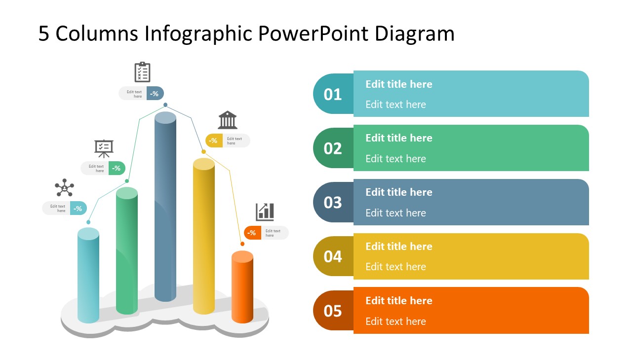
Represent column charts in a highly visual 3D format with this PPT template. A creative way to present data, this template is entirely editable, and we can craft either a one-page infographic or a series of slides explaining what we intend to disclose point by point.

3. Data Circles Infographic PowerPoint Template

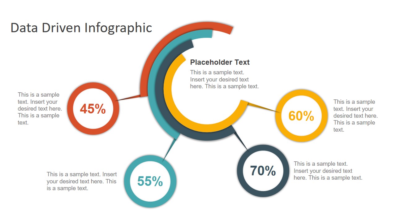
An alternative to the pie chart and donut chart diagrams, this template features a series of curved shapes with bubble callouts as ways of presenting data. Expand the information for each arch in the text placeholder areas.

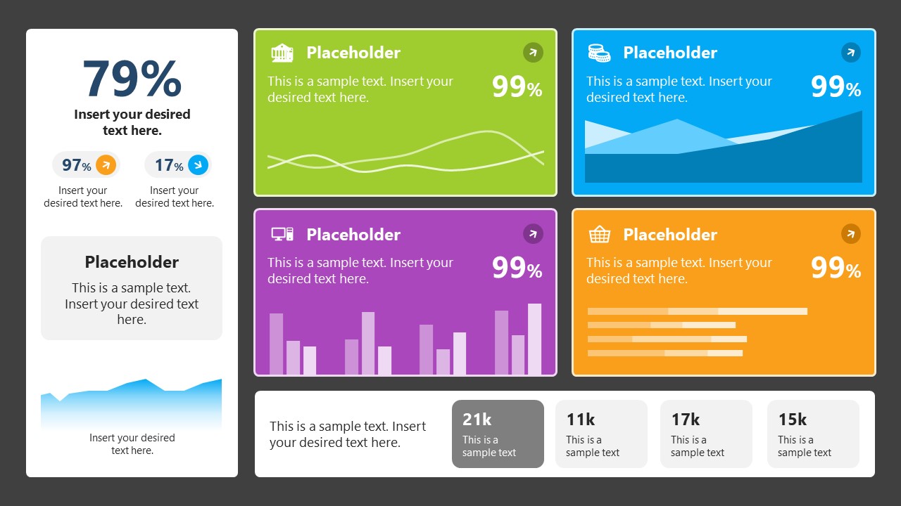
4. Colorful Metrics Dashboard for Data Presentation

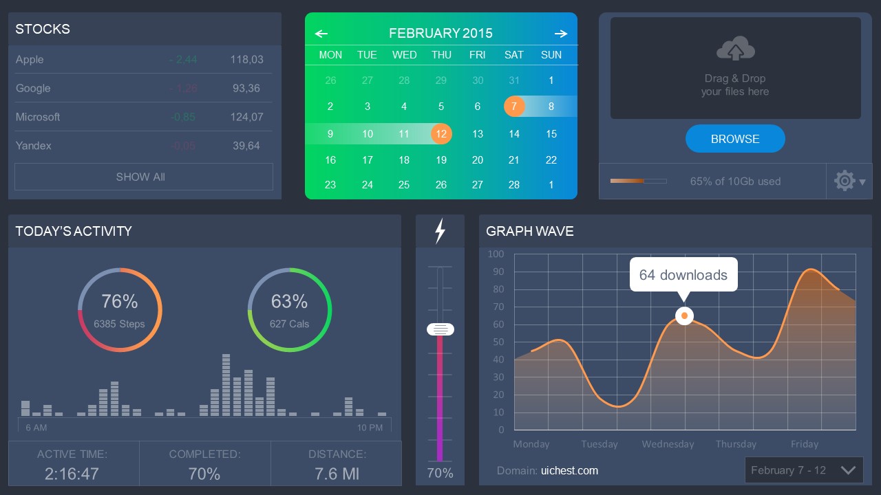
This versatile dashboard template helps us in the presentation of the data by offering several graphs and methods to convert numbers into graphics. Implement it for e-commerce projects, financial projections, project development, and more.

5. Animated Data Presentation Tools for PowerPoint & Google Slides

A slide deck filled with most of the tools mentioned in this article, from bar charts, column charts, treemap graphs, pie charts, histogram, etc. Animated effects make each slide look dynamic when sharing data with stakeholders.

6. Statistics Waffle Charts PPT Template for Data Presentations

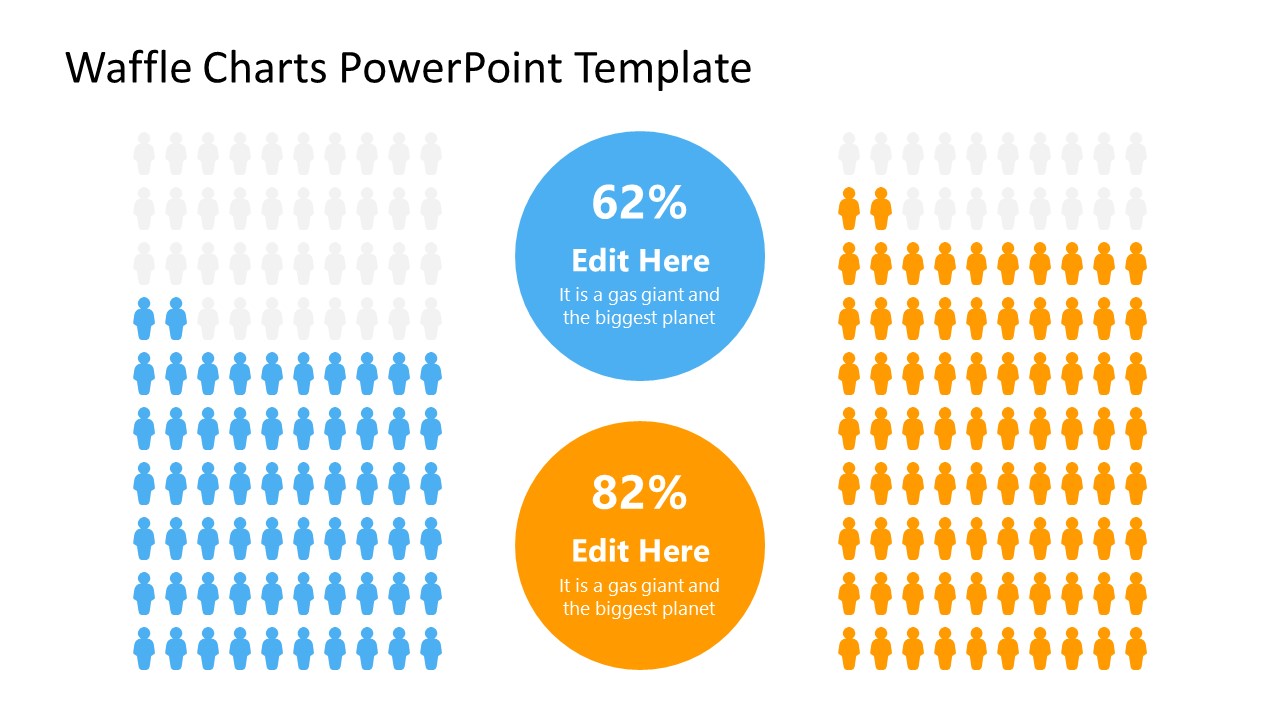
This PPT template helps us how to present data beyond the typical pie chart representation. It is widely used for demographics, so it’s a great fit for marketing teams, data science professionals, HR personnel, and more.

7. Data Presentation Dashboard Template for Google Slides

A compendium of tools in dashboard format featuring line graphs, bar charts, column charts, and neatly arranged placeholder text areas. 

8. Weather Dashboard for Data Presentation

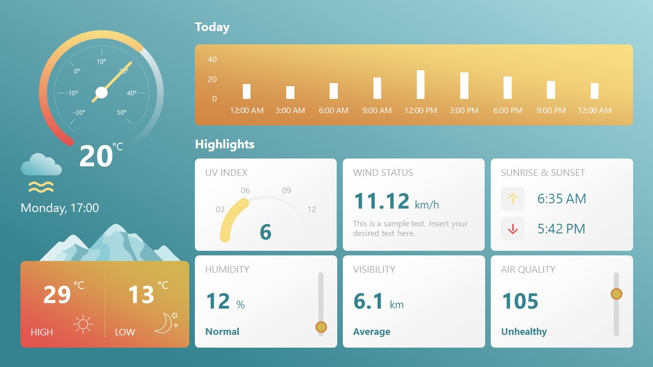
Share weather data for agricultural presentation topics, environmental studies, or any kind of presentation that requires a highly visual layout for weather forecasting on a single day. Two color themes are available.

9. Social Media Marketing Dashboard Data Presentation Template

Intended for marketing professionals, this dashboard template for data presentation is a tool for presenting data analytics from social media channels. Two slide layouts featuring line graphs and column charts.

10. Project Management Summary Dashboard Template

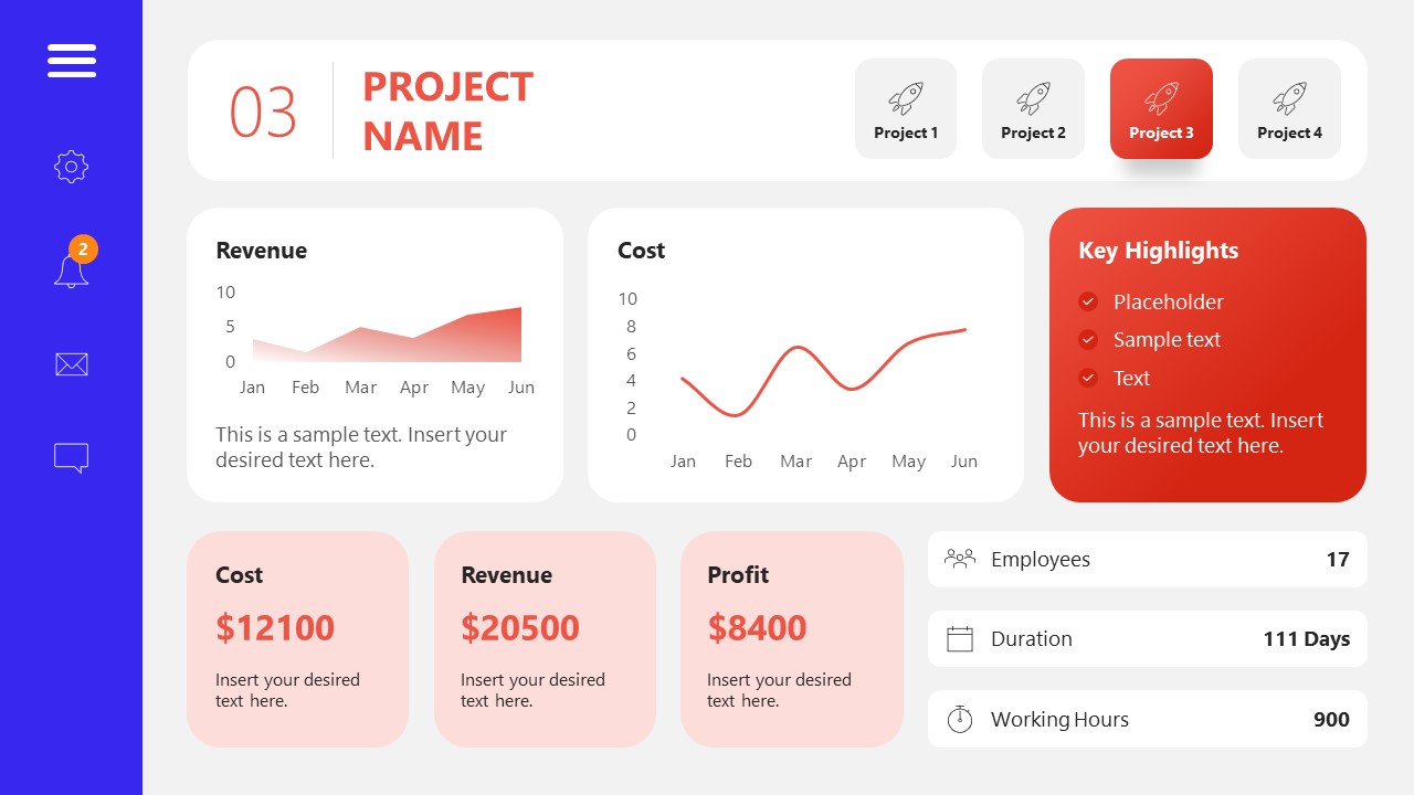
A tool crafted for project managers to deliver highly visual reports on a project’s completion, the profits it delivered for the company, and expenses/time required to execute it. 4 different color layouts are available.

11. Profit & Loss Dashboard for PowerPoint and Google Slides

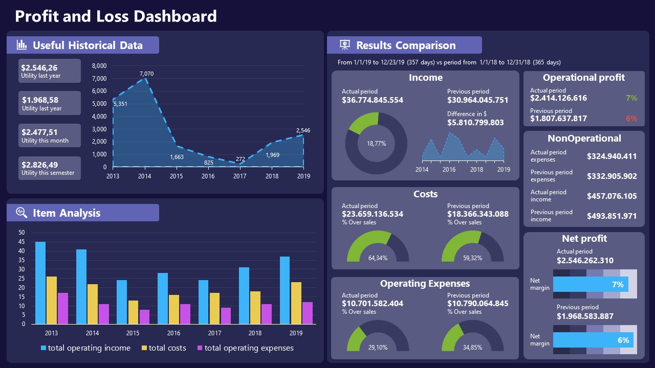
A must-have for finance professionals. This typical profit & loss dashboard includes progress bars, donut charts, column charts, line graphs, and everything that’s required to deliver a comprehensive report about a company’s financial situation.

Overwhelming visuals

One of the mistakes related to using data-presenting methods is including too much data or using overly complex visualizations. They can confuse the audience and dilute the key message.

Inappropriate chart types

Choosing the wrong type of chart for the data at hand can lead to misinterpretation. For example, using a pie chart for data that doesn’t represent parts of a whole is not right.

Lack of context

Failing to provide context or sufficient labeling can make it challenging for the audience to understand the significance of the presented data.

Inconsistency in design

Using inconsistent design elements and color schemes across different visualizations can create confusion and visual disarray.

Failure to provide details

Simply presenting raw data without offering clear insights or takeaways can leave the audience without a meaningful conclusion.

Lack of focus

Not having a clear focus on the key message or main takeaway can result in a presentation that lacks a central theme.

Visual accessibility issues

Overlooking the visual accessibility of charts and graphs can exclude certain audience members who may have difficulty interpreting visual information.

In order to avoid these mistakes in data presentation, presenters can benefit from using presentation templates . These templates provide a structured framework. They ensure consistency, clarity, and an aesthetically pleasing design, enhancing data communication’s overall impact.

Understanding and choosing data presentation types are pivotal in effective communication. Each method serves a unique purpose, so selecting the appropriate one depends on the nature of the data and the message to be conveyed. The diverse array of presentation types offers versatility in visually representing information, from bar charts showing values to pie charts illustrating proportions. 

Using the proper method enhances clarity, engages the audience, and ensures that data sets are not just presented but comprehensively understood. By appreciating the strengths and limitations of different presentation types, communicators can tailor their approach to convey information accurately, developing a deeper connection between data and audience understanding.

[1] Government of Canada, S.C. (2021) 5 Data Visualization 5.2 Bar Chart , 5.2 Bar chart .  https://www150.statcan.gc.ca/n1/edu/power-pouvoir/ch9/bargraph-diagrammeabarres/5214818-eng.htm

[2] Kosslyn, S.M., 1989. Understanding charts and graphs. Applied cognitive psychology, 3(3), pp.185-225. https://apps.dtic.mil/sti/pdfs/ADA183409.pdf

[3] Creating a Dashboard . https://it.tufts.edu/book/export/html/1870

[4] https://www.goldenwestcollege.edu/research/data-and-more/data-dashboards/index.html

[5] https://www.mit.edu/course/21/21.guide/grf-line.htm

[6] Jadeja, M. and Shah, K., 2015, January. Tree-Map: A Visualization Tool for Large Data. In GSB@ SIGIR (pp. 9-13). https://ceur-ws.org/Vol-1393/gsb15proceedings.pdf#page=15

[7] Heat Maps and Quilt Plots. https://www.publichealth.columbia.edu/research/population-health-methods/heat-maps-and-quilt-plots

[8] EIU QGIS WORKSHOP. https://www.eiu.edu/qgisworkshop/heatmaps.php

[9] About Pie Charts.  https://www.mit.edu/~mbarker/formula1/f1help/11-ch-c8.htm

[10] Histograms. https://sites.utexas.edu/sos/guided/descriptive/numericaldd/descriptiven2/histogram/ [11] https://asq.org/quality-resources/scatter-diagram

Like this article? Please share

Data Analysis, Data Science, Data Visualization Filed under Design

Related Articles

Filed under Design • March 27th, 2024

How to Make a Presentation Graph

Detailed step-by-step instructions to master the art of how to make a presentation graph in PowerPoint and Google Slides. Check it out!

Filed under Presentation Ideas • January 6th, 2024

All About Using Harvey Balls

Among the many tools in the arsenal of the modern presenter, Harvey Balls have a special place. In this article we will tell you all about using Harvey Balls.

Filed under Business • December 8th, 2023

How to Design a Dashboard Presentation: A Step-by-Step Guide

Take a step further in your professional presentation skills by learning what a dashboard presentation is and how to properly design one in PowerPoint. A detailed step-by-step guide is here!

Leave a Reply

• SUGGESTED TOPICS
• The Magazine
• Newsletters
• Managing Yourself
• Managing Teams
• Work-life Balance
• The Big Idea
• Data & Visuals
• Reading Lists
• Case Selections
• HBR Learning
• Topic Feeds
• Account Settings
• Email Preferences

Present Your Data Like a Pro

• Joel Schwartzberg

Demystify the numbers. Your audience will thank you.

While a good presentation has data, data alone doesn’t guarantee a good presentation. It’s all about how that data is presented. The quickest way to confuse your audience is by sharing too many details at once. The only data points you should share are those that significantly support your point — and ideally, one point per chart. To avoid the debacle of sheepishly translating hard-to-see numbers and labels, rehearse your presentation with colleagues sitting as far away as the actual audience would. While you’ve been working with the same chart for weeks or months, your audience will be exposed to it for mere seconds. Give them the best chance of comprehending your data by using simple, clear, and complete language to identify X and Y axes, pie pieces, bars, and other diagrammatic elements. Try to avoid abbreviations that aren’t obvious, and don’t assume labeled components on one slide will be remembered on subsequent slides. Every valuable chart or pie graph has an “Aha!” zone — a number or range of data that reveals something crucial to your point. Make sure you visually highlight the “Aha!” zone, reinforcing the moment by explaining it to your audience.

With so many ways to spin and distort information these days, a presentation needs to do more than simply share great ideas — it needs to support those ideas with credible data. That’s true whether you’re an executive pitching new business clients, a vendor selling her services, or a CEO making a case for change.

• JS Joel Schwartzberg oversees executive communications for a major national nonprofit, is a professional presentation coach, and is the author of Get to the Point! Sharpen Your Message and Make Your Words Matter and The Language of Leadership: How to Engage and Inspire Your Team . You can find him on LinkedIn and X. TheJoelTruth

Partner Center

Skills for Learning : Research Skills

Data analysis is an ongoing process that should occur throughout your research project. Suitable data-analysis methods must be selected when you write your research proposal. The nature of your data (i.e. quantitative or qualitative) will be influenced by your research design and purpose. The data will also influence the analysis methods selected.

We run interactive workshops to help you develop skills related to doing research, such as data analysis, writing literature reviews and preparing for dissertations. Find out more on the Skills for Learning Workshops page.

We have online academic skills modules within MyBeckett for all levels of university study. These modules will help your academic development and support your success at LBU. You can work through the modules at your own pace, revisiting them as required. Find out more from our FAQ What academic skills modules are available?

Quantitative data analysis

Broadly speaking, 'statistics' refers to methods, tools and techniques used to collect, organise and interpret data. The goal of statistics is to gain understanding from data. Therefore, you need to know how to:

• Produce data – for example, by handing out a questionnaire or doing an experiment.
• Organise, summarise, present and analyse data.
• Draw valid conclusions from findings.

There are a number of statistical methods you can use to analyse data. Choosing an appropriate statistical method should follow naturally, however, from your research design. Therefore, you should think about data analysis at the early stages of your study design. You may need to consult a statistician for help with this.

Tips for working with statistical data

• Plan so that the data you get has a good chance of successfully tackling the research problem. This will involve reading literature on your subject, as well as on what makes a good study.
• To reach useful conclusions, you need to reduce uncertainties or 'noise'. Thus, you will need a sufficiently large data sample. A large sample will improve precision. However, this must be balanced against the 'costs' (time and money) of collection.
• Consider the logistics. Will there be problems in obtaining sufficient high-quality data? Think about accuracy, trustworthiness and completeness.
• Statistics are based on random samples. Consider whether your sample will be suited to this sort of analysis. Might there be biases to think about?
• How will you deal with missing values (any data that is not recorded for some reason)? These can result from gaps in a record or whole records being missed out.
• When analysing data, start by looking at each variable separately. Conduct initial/exploratory data analysis using graphical displays. Do this before looking at variables in conjunction or anything more complicated. This process can help locate errors in the data and also gives you a 'feel' for the data.
• Look out for patterns of 'missingness'. They are likely to alert you if there’s a problem. If the 'missingness' is not random, then it will have an impact on the results.
• Be vigilant and think through what you are doing at all times. Think critically. Statistics are not just mathematical tricks that a computer sorts out. Rather, analysing statistical data is a process that the human mind must interpret!

Top tips! Try inventing or generating the sort of data you might get and see if you can analyse it. Make sure that your process works before gathering actual data. Think what the output of an analytic procedure will look like before doing it for real.

(Note: it is actually difficult to generate realistic data. There are fraud-detection methods in place to identify data that has been fabricated. So, remember to get rid of your practice data before analysing the real stuff!)

Statistical software packages

Software packages can be used to analyse and present data. The most widely used ones are SPSS and NVivo.

SPSS is a statistical-analysis and data-management package for quantitative data analysis. Click on ‘ How do I install SPSS? ’ to learn how to download SPSS to your personal device. SPSS can perform a wide variety of statistical procedures. Some examples are:

• Data management (i.e. creating subsets of data or transforming data).
• Summarising, describing or presenting data (i.e. mean, median and frequency).
• Looking at the distribution of data (i.e. standard deviation).
• Comparing groups for significant differences using parametric (i.e. t-test) and non-parametric (i.e. Chi-square) tests.
• Identifying significant relationships between variables (i.e. correlation).

NVivo can be used for qualitative data analysis. It is suitable for use with a wide range of methodologies. Click on ‘ How do I access NVivo ’ to learn how to download NVivo to your personal device. NVivo supports grounded theory, survey data, case studies, focus groups, phenomenology, field research and action research.

• Process data such as interview transcripts, literature or media extracts, and historical documents.
• Code data on screen and explore all coding and documents interactively.
• Rearrange, restructure, extend and edit text, coding and coding relationships.
• Search imported text for words, phrases or patterns, and automatically code the results.

Qualitative data analysis

Miles and Huberman (1994) point out that there are diverse approaches to qualitative research and analysis. They suggest, however, that it is possible to identify 'a fairly classic set of analytic moves arranged in sequence'. This involves:

• Affixing codes to a set of field notes drawn from observation or interviews.
• Noting reflections or other remarks in the margins.
• Sorting/sifting through these materials to identify: a) similar phrases, relationships between variables, patterns and themes and b) distinct differences between subgroups and common sequences.
• Isolating these patterns/processes and commonalties/differences. Then, taking them out to the field in the next wave of data collection.
• Highlighting generalisations and relating them to your original research themes.
• Taking the generalisations and analysing them in relation to theoretical perspectives.

        (Miles and Huberman, 1994.)

Patterns and generalisations are usually arrived at through a process of analytic induction (see above points 5 and 6). Qualitative analysis rarely involves statistical analysis of relationships between variables. Qualitative analysis aims to gain in-depth understanding of concepts, opinions or experiences.

Presenting information

There are a number of different ways of presenting and communicating information. The particular format you use is dependent upon the type of data generated from the methods you have employed.

Here are some appropriate ways of presenting information for different types of data:

Bar charts: These   may be useful for comparing relative sizes. However, they tend to use a large amount of ink to display a relatively small amount of information. Consider a simple line chart as an alternative.

Pie charts: These have the benefit of indicating that the data must add up to 100%. However, they make it difficult for viewers to distinguish relative sizes, especially if two slices have a difference of less than 10%.

Other examples of presenting data in graphical form include line charts and  scatter plots .

Qualitative data is more likely to be presented in text form. For example, using quotations from interviews or field diaries.

• Plan ahead, thinking carefully about how you will analyse and present your data.
• Think through possible restrictions to resources you may encounter and plan accordingly.
• Find out about the different IT packages available for analysing your data and select the most appropriate.
• If necessary, allow time to attend an introductory course on a particular computer package. You can book SPSS and NVivo workshops via MyHub .
• Code your data appropriately, assigning conceptual or numerical codes as suitable.
• Organise your data so it can be analysed and presented easily.
• Choose the most suitable way of presenting your information, according to the type of data collected. This will allow your information to be understood and interpreted better.

Primary, secondary and tertiary sources

Information sources are sometimes categorised as primary, secondary or tertiary sources depending on whether or not they are ‘original’ materials or data. For some research projects, you may need to use primary sources as well as secondary or tertiary sources. However the distinction between primary and secondary sources is not always clear and depends on the context. For example, a newspaper article might usually be categorised as a secondary source. But it could also be regarded as a primary source if it were an article giving a first-hand account of a historical event written close to the time it occurred.

• Primary sources
• Secondary sources
• Tertiary sources
• Grey literature

Primary sources are original sources of information that provide first-hand accounts of what is being experienced or researched. They enable you to get as close to the actual event or research as possible. They are useful for getting the most contemporary information about a topic.

Examples include diary entries, newspaper articles, census data, journal articles with original reports of research, letters, email or other correspondence, original manuscripts and archives, interviews, research data and reports, statistics, autobiographies, exhibitions, films, and artists' writings.

Some information will be available on an Open Access basis, freely accessible online. However, many academic sources are paywalled, and you may need to login as a Leeds Beckett student to access them. Where Leeds Beckett does not have access to a source, you can use our  Request It! Service .

Secondary sources interpret, evaluate or analyse primary sources. They're useful for providing background information on a topic, or for looking back at an event from a current perspective. The majority of your literature searching will probably be done to find secondary sources on your topic.

Examples include journal articles which review or interpret original findings, popular magazine articles commenting on more serious research, textbooks and biographies.

The term tertiary sources isn't used a great deal. There's overlap between what might be considered a secondary source and a tertiary source. One definition is that a tertiary source brings together secondary sources.

Examples include almanacs, fact books, bibliographies, dictionaries and encyclopaedias, directories, indexes and abstracts. They can be useful for introductory information or an overview of a topic in the early stages of research.

Depending on your subject of study, grey literature may be another source you need to use. Grey literature includes technical or research reports, theses and dissertations, conference papers, government documents, white papers, and so on.

Artificial intelligence tools

Before using any generative artificial intelligence or paraphrasing tools in your assessments, you should check if this is permitted on your course.

If their use is permitted on your course, you must  acknowledge any use of generative artificial intelligence tools  such as ChatGPT or paraphrasing tools (e.g., Grammarly, Quillbot, etc.), even if you have only used them to generate ideas for your assessments or for proofreading.

• Academic Integrity Module in MyBeckett
• Assignment Calculator
• Building on Feedback
• Disability Advice
• Essay X-ray tool
• International Students' Academic Introduction
• Manchester Academic Phrasebank
• Quote, Unquote
• Skills and Subject Suppor t
• Turnitin Grammar Checker

{{You can add more boxes below for links specific to this page [this note will not appear on user pages] }}

• Research Methods Checklist
• Sampling Checklist

Skills for Learning FAQs

0113 812 1000

• University Disclaimer
• Accessibility

• school Campus Bookshelves
• menu_book Bookshelves
• perm_media Learning Objects
• login Login
• how_to_reg Request Instructor Account
• hub Instructor Commons

Margin Size

• Download Page (PDF)
• Download Full Book (PDF)
• Periodic Table
• Physics Constants
• Scientific Calculator
• Reference & Cite
• Tools expand_more
• Readability

selected template will load here

This action is not available.

1.3: Presentation of Data

• Last updated
• Save as PDF
• Page ID 577

\( \newcommand{\vecs}[1]{\overset { \scriptstyle \rightharpoonup} {\mathbf{#1}} } \)

\( \newcommand{\vecd}[1]{\overset{-\!-\!\rightharpoonup}{\vphantom{a}\smash {#1}}} \)

\( \newcommand{\id}{\mathrm{id}}\) \( \newcommand{\Span}{\mathrm{span}}\)

( \newcommand{\kernel}{\mathrm{null}\,}\) \( \newcommand{\range}{\mathrm{range}\,}\)

\( \newcommand{\RealPart}{\mathrm{Re}}\) \( \newcommand{\ImaginaryPart}{\mathrm{Im}}\)

\( \newcommand{\Argument}{\mathrm{Arg}}\) \( \newcommand{\norm}[1]{\| #1 \|}\)

\( \newcommand{\inner}[2]{\langle #1, #2 \rangle}\)

\( \newcommand{\Span}{\mathrm{span}}\)

\( \newcommand{\id}{\mathrm{id}}\)

\( \newcommand{\kernel}{\mathrm{null}\,}\)

\( \newcommand{\range}{\mathrm{range}\,}\)

\( \newcommand{\RealPart}{\mathrm{Re}}\)

\( \newcommand{\ImaginaryPart}{\mathrm{Im}}\)

\( \newcommand{\Argument}{\mathrm{Arg}}\)

\( \newcommand{\norm}[1]{\| #1 \|}\)

\( \newcommand{\Span}{\mathrm{span}}\) \( \newcommand{\AA}{\unicode[.8,0]{x212B}}\)

\( \newcommand{\vectorA}[1]{\vec{#1}}      % arrow\)

\( \newcommand{\vectorAt}[1]{\vec{\text{#1}}}      % arrow\)

\( \newcommand{\vectorB}[1]{\overset { \scriptstyle \rightharpoonup} {\mathbf{#1}} } \)

\( \newcommand{\vectorC}[1]{\textbf{#1}} \)

\( \newcommand{\vectorD}[1]{\overrightarrow{#1}} \)

\( \newcommand{\vectorDt}[1]{\overrightarrow{\text{#1}}} \)

\( \newcommand{\vectE}[1]{\overset{-\!-\!\rightharpoonup}{\vphantom{a}\smash{\mathbf {#1}}}} \)

Learning Objectives

• To learn two ways that data will be presented in the text.

In this book we will use two formats for presenting data sets. The first is a data list, which is an explicit listing of all the individual measurements, either as a display with space between the individual measurements, or in set notation with individual measurements separated by commas.

Example \(\PageIndex{1}\)

The data obtained by measuring the age of \(21\) randomly selected students enrolled in freshman courses at a university could be presented as the data list:

\[\begin{array}{cccccccccc}18 & 18 & 19 & 19 & 19 & 18 & 22 & 20 & 18 & 18 & 17 \\ 19 & 18 & 24 & 18 & 20 & 18 & 21 & 20 & 17 & 19 &\end{array} \nonumber \]

or in set notation as:

\[ \{18,18,19,19,19,18,22,20,18,18,17,19,18,24,18,20,18,21,20,17,19\} \nonumber \]

A data set can also be presented by means of a data frequency table, a table in which each distinct value \(x\) is listed in the first row and its frequency \(f\), which is the number of times the value \(x\) appears in the data set, is listed below it in the second row.

Example \(\PageIndex{2}\)

The data set of the previous example is represented by the data frequency table

\[\begin{array}{c|cccccc}x & 17 & 18 & 19 & 20 & 21 & 22 & 24 \\ \hline f & 2 & 8 & 5 & 3 & 1 & 1 & 1\end{array} \nonumber \]

The data frequency table is especially convenient when data sets are large and the number of distinct values is not too large.

Key Takeaway

• Data sets can be presented either by listing all the elements or by giving a table of values and frequencies.

Academia.edu no longer supports Internet Explorer.

To browse Academia.edu and the wider internet faster and more securely, please take a few seconds to  upgrade your browser .

Enter the email address you signed up with and we'll email you a reset link.

• We're Hiring!
• Help Center

Chapter 4 PRESENTATION, ANALYSIS AND INTERPRETATION OF DATA

Related Papers

SMCC Higher Education Research Journal

Gian Venci Alonzo

International Journal of Research -GRANTHAALAYAH

Sherill A . Gilbas

This paper highlights the trust, respect, safety and security ratings of the community to the Philippine National Police (PNP) in the Province of Albay. It presents the sectoral ratings to PNP programs. The survey utilized a structured interview with 200 sample respondents from Albay coming from different sectors. Male respondents outnumbered female respondents. The majority of the respondents are 41-50 years old, at least high school graduates and are married. The respondents gave the highest net rating on respect, followed by net rating on trust and the lowest net rating on safety and security on the performance of the PNP. Moreover, a high net rating on commitment of support to the identified programs of the PNP was also attained from the respondents. The highest net rating of support is given to the PNP’s anti-illegal drugs program, followed by anti-terrorism, anti-riding in tandem and anti-illegal gambling programs. The ratings of the PNP obtained from the different sectors of...

Charlie Rosales

IOER International Multidisciplinary Research Journal

IOER International Multidisciplinary Research Journal ( IIMRJ)

Police organizations have conducted operational activities to reduce the opportunity for would-be criminals to commit crimes. This operational activity includes patrol, traffic management, and investigation. In this study, the extent of police operational activities in Pagadian City, Zamboanga del Sur, Philippines, was evaluated to determine the extent of police operational activities and to test the association between the crime rate and the extent of police operation activities. This study utilized a quantitative descriptive research method. The respondents were 142 active police officers who were chosen purposively by employing total enumeration. The gathering of data was done using a self-made questionnaire, which underwent validation and reliability testing. The statistical tools used were frequency count, mean computation, percentage, and regression analysis. The results revealed that more respondents were 31-35 years old and above. Most of them were male, bachelor's degree holders, attended training and seminars for 50 hours, and served the police force for 15 years and below. Patrolling and investigation were found to be much observable while traffic management was observable. As for index crime, there were more crimes against the person committed than crimes against property. As for non-index crimes, there were more other non-index crimes compared to the violation of special laws. Patrolling has a positive influence on the commission and non-commission of both index and non-index crimes. This study also recommends intensive patrolling on hot-spot areas for criminal presence and activity, strengthening traffic management practices, procurement of traffic lights, improving traffic signs, and intensive implementation of traffic laws and regulations.

International Journal of Social Sciences and Humanities Research

Bro. Jose Arnold L . Alferez, OCDS

Effective law enforcement service demands that the law enforcement officers are diligent and effective in their duties and responsibilities. They should be punctual and alert while on their respective beats. They should respect the human rights of the people of the community they serve. They should even patrol their beats on foot so that their visibility would be more evident thus curtailing the criminal impulses of the criminally inclined, instead of whisking through the vicinity on the " flying visit" to their assigned places without even giving the people a glimpse of their presence. Transparency is the call of effective law enforcement service. However, effective law enforcement necessitates that the police command should be provided police equipment like two-way radios so that they could readily call for assistance whenever necessary, in order to improve the delivery of services and the maintenance of peace and order. Furthermore, a strong partnership between the police and the community will help ensure the success of the Philippine National Police in its drive against criminality. The findings of this study showed that the police force of the municipality of Pinamungajan, Cebu did their best under the circumstances they had to work in, but their efforts were not equally recognized by the people of the community. Hence, the need for support from the local officials and the people in the community are important factors that would facilitate the effectiveness of the law enforcement service.

Filius Populi

The Philippine National Police has implemented the new rank classification and abbreviation that shall be used in all manner of organization communications. Interview method was used to gather the information from the PNP RCADD respondents and selected community residents. Focus Group Discussion was conducted among the Barangay Officials to validate the data gathered. The findings of the study as follows: The respondents were not fully aware yet on the modified new rank classification applied in the PNP organization today; They shared diverse insights both positive and negative about the PNP modified new rank classification and it can offer a positive outcome in the long-run . Respondents were satisfied with the implementation of the PNP community relations program under the new rank classification. However, the modified new rank classification of the PNP would have the following positive implications: The new rank would mean higher people’s expectations; bring new image of the PNP;...

josefina B A L U C A N A G bitonio

DISSERTATION ABSTRACT Title : THE WOMEN AND CHILDREN PROTECTION SERVICES OF THE PHILIPPINE NATIONAL POLICE-CORDILLERA ADMINISTRATIVE REGION Researcher : MELY RITA D. ANAMONG-DAVIS Institution : Lyceum-Northwestern University, Dagupan City Degree : DOCTOR IN PUBLIC ADMINISTRATION Date : April 5, 2013 Abstract : This research sought to evaluate the provision of services provided by the members of the Women and Children Protection Desk of the Philippine National Police (PNP) Cordillera Administrative Region . The descriptive-evaluative research design was used in this study with the questionnaire, interviews as the data- gathering tool in the evaluation of the WCPD of the PNP services rendered to the victims-survivors of violence in the Cordillera Region. The types and statistics of cases investigated by the members of the WCPD of the PNP in the Cordillera were provided by the different offices of the WCPD of the PNP particularly the Regional and Provincial Offices. On the other hand, the acquired data from the respondents describes the capability of the WCPD office and personnel, relative to the organizational structure, financial resources, human resources, equipment and facilities; the extent of the mandated services provided for the victims-survivors of violence, level of satisfaction of the WCPD clientele and the problems encountered by the members of the WCPD of the PNP in providing the services to its clientele. Based on the findings, a proposal were formulated to enhance the quality or quantity of the services rendered to the victims of abuses and violence. Two hundred thirty (230) respondents were employed to answer the questionnaire to get the needed data, 160 from the police officers and 70 from the clientele of the WCPD. In the treatment of the data, SPSS version 20 was used in the analysis of data, Paired t-test for the determination of the significant difference in the perceptions of the two groups of respondents on the extent of provision of the mandated services by the WCPD of the PNP in the Cordillera and Spearman rank correlation for determining the level of satisfaction of the victims-survivors related to their perception on the extent of services provided by the Women and Children Protection Desk of the PNP. The findings of the study were the following: 1) Cases handled by the members of the WCPD of the PNP are physical injuries, violation of RA 9262, Rape and Acts of lasciviousness are the myriad cases committed against women; for crimes against children, rape, physical injuries, other forms of RA 7610 and acts of lasciviousness ; and for the crimes committed by the Children in Conflict with the law theft and robbery for intent to gain and material gain, physical injuries, rape and acts of lasciviousness are the majority they committed. The fact of this case is that 16 children were involved in the commission of rape where the youngest perpetrator is 7 years old. 2. On the capability of the members of the WCPD of the PNP, police officers believed that WCPD investigators are capable in providing the services to the victims of violence while the clientele respondents states otherwise that on some point along capability on human resources states that the number of police women assigned with the WCPD of the PNP is not sufficient to provide the services to its clientele. 3. On the extent of the mandated services provided to the victims-survivors of violence by the members of the WCPD of the PNP, perceptions of the police officers that to a great extent the members of the WCPD provide the services while the perceptions of the clientele is just on average extent on the services provided to them. 3.1. On the significant difference in the perceptions of the two groups of respondent on the extent of provision of the mandated services by the WCPD of the PNP in the Cordillera, there is a significant difference in the perception of the two groups of respondents on the extent of mandated services provided by the WCPD of the PNP in the Cordillera. The result indicates that the performance of the WCPD in rendering service is inadequate in the perception of its clients. 4) The satisfaction level of the clientele on the extent of services provided by the WCPD of the PNP is just moderate. This validates the result of the extent of the mandated services provided to the victims-survivors of violence by the WCPD investigators to be just on average. 5. On the level of satisfaction of the victims-survivors related to their perception on the extent of services provided by the Women and Children Protection Desk of the PNP revealed that WCPD clients is higher with greater extent of services being rendered by the WCPD. It indicates that the WCPD of the PNP in Cordillera should strive more to really fulfill the needed services to be provided with its clients. Likewise, on the level of satisfaction of the victims-survivors related to the capability of the WCPD of the PNP Cordillera in providing their mandated services disclosed that the more capable of the WCPD of the PNP in Cordillera will definitely provide an intense delivery of services to its clients. 7) Lastly, for the problems encountered by the WCPD of the PNP in providing services the following are considered a) no imagery tool kit purposely for the children’s victim to illicit information regarding the incident; b) the insufficient number of female police officers to investigate cases of women and children; c) lack of training of WCPD officers in handling VAWC cases and other gender-based crimes and d) service vehicle purposely for WCPD use only. Based on the findings and conclusion, the following recommendations are offered. 1. The propose strategies to enhance the services provided to the victims-survivors by the WCPD investigators must be intensely implemented: 1.a. There should be budgetary allocations for WCPD to enhance their capability to provide services and to fulfill the satisfaction of their clientele. 1.b. Increase the number of the female police officers assigned with the WCPD to sustain the 24/7 availability of investigators. 1.c. There should be a continuous conduct of specialized training on the Investigation of Crimes involving Women and children to all WCPD officers to include policemen for conclusive delivery of services for the victims of violence. 1.d. Purchase of the imagery tool kit purposely for the children’s victim of sexual abuse to illicit information regarding the incident.1.e. Issuance of service vehicle purposely for the Women and Children Protection Desk.1.f. Provide computer sets for WCPD.1.g. Provide communication equipment to be issued with the WCPD. 1.h. To improve the quality and consistency of WCPD services, a constant monitoring scheme and or clientele feedback should be implemented to understand the ways that service can be improved. 1.i. Develop and sustain the collaborative effort of the multidisciplinary team to meet the specific protocol designed to meet the needs of the victims of violence.1.j. To prevent new victims of violence, there should be a persistent campaign through advocacy and the education of the community in every barangay in coordination with the different member agencies. 2. A follow-up study should be conducted to cover other areas particularly target respondents on the level of satisfaction on the services provided for the victims of violence which is the main purpose of the establishment of the Women and Children Protection Desk.

Maita P Guadamor

RELATED PAPERS

eleonora trivellin

Physics Letters B

E. Tuominen

Silvia Paladino

The Journal of Chemical Physics

Tonu Reinot

Revista Sophia Universidad La Gran Colombia

Elizabeth Ormart

Edições Nosso Conhecimento

Aamir Al-Mosawi

British Journal of Surgery

Peter Loizou

Jane Lethbridge

Wolfgang Calmano

Claudio Mahler

International Journal of Intelligent Engineering and Systems

khamla nonalinsavath

Scientific Reports

Natalia Olovnikova

Teresa Otero

Cvetka Grasic Kuhar

Journal of General Virology

Samir Casseb

Kingsley Agho

Paula andrea Trejos arias

International Journal of Impact Engineering

Daniel McCrum

怎么购买美国亚利桑那大学毕业证 ua学位证书硕士文凭证书GRE成绩单原版一模一样

安大略理工大学毕业证书 购买加拿大学历UOI文凭学位证书成绩单

•   We're Hiring!
•   Help Center
• Find new research papers in:
• Health Sciences
• Earth Sciences
• Cognitive Science
• Mathematics
• Computer Science
• Academia ©2024

Introduction to Data Analysis

Apr 06, 2019

2.59k likes | 6k Views

Introduction to Data Analysis. Data Measurement Measurement of the data is the first step in the process that ultimately guides the final analysis. Consideration of sampling, controls, errors (random and systematic) and the required precision all influence the final analysis.

Share Presentation

• central limit theorem
• normal distributions
• determination
• univariate analysis skewed distributions
• column chart
• time period

Presentation Transcript

Introduction to Data Analysis • Data Measurement • Measurement of the data is the first step in the process that ultimately guides the final analysis. • Consideration of sampling, controls, errors (random and systematic) and the required precision all influence the final analysis. • Validation: Instruments and methods used to measure the data must be validated for accuracy. • Precision and accuracy…Determination of error • Social vs. Physical Sciences

Introduction to Data Analysis • Types of data • Univariate/Multivariate • Univariate: When we use one variable to describe a person, place, or thing. • Multivariate: When we use two or more variables to measure a person, place or thing. Variables may or may not be dependent on each other. • Cross-sectional data/Time-ordered data (business, social sciences) • Cross-Sectional: Measurements taken at one time period • Time-Ordered: Measurements taken over time in chronological sequence. • The type of data will dictate (in part) the appropriate data-analysis method.

Introduction to Data Analysis • Measurement Scales • Nominal or Categorical Scale • Classification of people, places, or things into categories (e.g. age ranges, colors, etc.). • Classifications must be mutually exclusive (every element should belong to one category with no ambiguity). • Weakest of the four scales. No category is greater than or less (better or worse) than the others. They are just different. • Ordinal or Ranking Scale • Classification of people, places, or things into a ranking such that the data is arranged into a meaningful order (e.g. poor, fair, good, excellent). • Qualitative classification only

Introduction to Data Analysis • Measurement Scales (business, social sciences) • Interval Scale • Data classified by ranking. • Quantitative classification (time, temperature, etc). • Zero point of scale is arbitrary (differences are meaningful). • Ratio Scale • Data classified as the ratio of two numbers. • Quantitative classification (height, weight, distance, etc). • Zero point of scale is real (data can be added, subtracted, multiplied, and divided).

Univariate Analysis/Descriptive Statistics • Descriptive Statistics • The Range • Min/Max • Average • Median • Mode • Variance • Standard Deviation • Histograms and Normal Distributions

Distributions Descriptive statistics are easier to interpret when graphically illustrated. However, charting each data element can lead to very busy and confusing charts that do not help interpret the data. Grouping the data elements into categories and charting the frequency within these categories yields a graphical illustration of how the data is distributed throughout its range. Univariate Analysis/Histograms

Univariate Analysis/Histograms With just a few columns this chart is difficult to interpret. It tells you very little about the data set. Even finding the Min and Max can be difficult. The data can be presented such that more statistical parameters can be estimated from the chart (average, standard deviation).

Univariate Analysis/Histograms • Frequency Table • The first step is to decide on the categories and group the data appropriately. (45, 49, 50, 53, 60, 62, 63, 65, 66, 67, 69, 71, 73, 74, 74, 78, 81, 85, 87, 100)

Univariate Analysis/Histograms • Histogram • A histogram is simply a column chart of the frequency table.

Histogram Univariate Analysis/Histograms Average (68.6) and Median (68) Mode (74) -1SD +1SD

Univariate Analysis/Normal Distributions • Distributions that can be described mathematically as Gaussian are also called Normal • The Bell curve • Symmetrical • Mean ≈ Median Mean, Median, Mode

Univariate Analysis/Skewed Distributions • When data are skewed, the mean and SD can be misleading • Skewness sk= 3(mean-median)/SD If sk>|1| then distribution is non-symetrical • Negatively skewed • Mean<Median • Sk is negative • Positively Skewed • Mean>Median • Sk is positive

Central Limit Theorem • Regardless of the shape of a distribution, the distribution of the sample mean based on samples of size N approaches a normal curve as N increases. • N must be less than the entire sample N=10

Univariate Analysis/Descriptive Statistics • The Range • Difference between minimum and maximum values in a data set • Larger range usually (but not always) indicates a large spread or deviation in the values of the data set. (73, 66, 69, 67, 49, 60, 81, 71, 78, 62, 53, 87, 74, 65, 74, 50, 85, 45, 63, 100)

Univariate Analysis/Descriptive Statistics • The Average (Mean) • Sum of all values divided by the number of values in the data set. • One measure of central location in the data set. Average = Average=(73+66+69+67+49+60+81+71+78+62+53+87+74+65+74+50+85+45+63+100)/20 = 68.6 Excel function: AVERAGE()

The data may or may not be symmetrical around its average value 0 2.5 7.5 10 4.8 0 2.5 7.5 10 4.8 Univariate Analysis/Descriptive Statistics

The Median The middle value in a sorted data set. Half the values are greater and half are less than the median. Another measure of central location in the data set. (45, 49, 50, 53, 60, 62, 63, 65, 66, 67, 69, 71, 73, 74, 74, 78, 81, 85, 87, 100) Median: 68 (1, 2, 4, 7, 8, 9, 9) Excel function: MEDIAN() Univariate Analysis/Descriptive Statistics

The Median May or may not be close to the mean. Combination of mean and median are used to define the skewness of a distribution. 0 2.5 7.5 10 6.25 Univariate Analysis/Descriptive Statistics

The Mode Most frequently occurring value. Another measure of central location in the data set. (45, 49, 50, 53, 60, 62, 63, 65, 66, 67, 69, 71, 73, 74, 74, 78, 81, 85, 87, 100) Mode: 74 Generally not all that meaningful unless a larger percentage of the values are the same number. Univariate Analysis/Descriptive Statistics

Univariate Analysis/Descriptive Statistics • Variance • One measure of dispersion (deviation from the mean) of a data set. The larger the variance, the greater is the average deviation of each datum from the average value. Variance = Average value of the data set Variance = [(45 – 68.6)2 + (49 – 68.6)2 + (50 – 68.6)2 + (53 – 68.6)2 + …]/20 = 181 Excel Functions: VARP(), VAR()

Standard Deviation Square root of the variance. Can be thought of as the average deviation from the mean of a data set. The magnitude of the number is more in line with the values in the data set. Univariate Analysis/Descriptive Statistics Standard Deviation = ([(45 – 68.6)2 + (49 – 68.6)2 + (50 – 68.6)2 + (53 – 68.6)2 + …]/20)1/2 = 13.5 Excel Functions: STDEVP(), STDEV()

• More by User

Introduction to Secondary Data Analysis

Introduction to Secondary Data Analysis. Young Ik Cho, PhD Research Associate Professor Survey Research Laboratory University of Illinois at Chicago Fall, 2009. Data collected by a person or organization other than the users of the data. What is secondary data?.

1.02k views • 27 slides

Introduction to Survey Data Analysis

Introduction to Survey Data Analysis. Linda K. Owens, PhD Assistant Director for Sampling &amp; Analysis Survey Research Laboratory University of Illinois at Chicago. Focus of the seminar. Data cleaning/missing data Sampling bias reduction. When analyzing survey data.

625 views • 29 slides

Introduction to Data Analysis. Why do we analyze data? Make sense of data we have collected Basic steps in preliminary data analysis Editing Coding Tabulating. Introduction to Data Analysis. Editing of data Impose minimal quality standards on the raw data

756 views • 21 slides

Introduction to Data analysis

Introduction to Data analysis. IGOR Pro Version 6.1 01-24-2012. Features of Igor-What Igor can do. Igor Pro is an integrated program for visualizing, analyzing, transforming and presenting experimental data. Features of Igor Pro includes: Publication – quality graphics

638 views • 27 slides

Introduction to Data Analysis.

Introduction to Data Analysis. Multivariate Linear Regression. Last week’s lecture. Simple model of how one interval level variable affects another interval level variable. A predictive and causal model. We have an independent variable ( X ) that predicts a dependent variable ( Y ).

655 views • 53 slides

Introduction to Data Analysis. Sampling. Today’s lecture. Sampling (A&amp;F 2) Why sample? Random sampling. Other sampling methods. Stata stuff in Lab. Sampling introduction. Last week we were talking about populations (albeit in some cases small ones, such as my friends).

532 views • 17 slides

Introduction to Data Analysis. Probability Confidence Intervals. Today’s lecture. Some stuff on probability Confidence intervals (A&amp;F 5). Standard error (part 2) and efficiency. Confidence intervals for means. Confidence intervals for proportions. Last week’s aide memoire.

991 views • 80 slides

Introduction to Data Analysis. Downloading CasaXPS Online tutorials, resources, manuals, videos Low resolution analysis, calculating atomic % File Handling, report generation (slide 7) High resolution analysis Peak fits (Gaussian-Lorentzian, Voigt, Doniach-Sunjic) Atomic % (tags)

313 views • 14 slides

831 views • 80 slides

Introduction to Data Analysis. Introduction to Logistic Regression. This week’s lecture. Categorical dependent variables in more complicated models. Logistic regression (for binary categorical dependent variables). Why can’t we just use OLS? How does logistic regression work?

465 views • 45 slides

Introduction to Data Analysis. Hypothesis Testing for means and proportions. Today’s lecture. Hypothesis testing (A&amp;F 6) What’s a hypothesis? Probabilities of hypotheses being correct. Type I and type II errors. What’s a hypothesis?. Hypotheses = testable statements about the world.

471 views • 30 slides

Introduction to Data Analysis. Confidence Intervals. Standard errors continued…. Last week we managed to work out some info about the distribution of sample means. If we have lots of samples then: Mean of all the sample means = population mean.

538 views • 51 slides

Introduction to Longitudinal Data Analysis

Introduction to Longitudinal Data Analysis. Robert J. Gallop West Chester University 24 June 2010 ACBS- Reno, NV. Longitudinal Data Analysis. Part 1 - Primitive Approach. Mathematician mentality.

2.17k views • 176 slides

Introduction to Data Analysis. Sampling and Probability Distributions. Today’s lecture. Sampling(A&amp;F 2) Why sample Sampling methods Probability distributions (A&amp;F 4) Normal distribution. Sampling distributions = normal distributions. Standard errors (part 1). Sampling introduction.

503 views • 46 slides

Introduction to Data Analysis. Non-linearity, heteroskedasticity, multicollinearity, oh my!. Last week’s lecture. Extended our linear regression model to include: Multiple independent variables (so as to get rid of spurious relationships)

588 views • 50 slides

259 views • 14 slides

Introduction to RHESSI Data Analysis

Introduction to RHESSI Data Analysis. Documentation Data Products Access to Data SSW Analysis Modes RHESSI GUI Combining GUI and Command Line RHESSI Objects Details and Links for these topics. Documentation RHESSI Data and Software Center Web Page

215 views • 17 slides

Thank you for visiting nature.com. You are using a browser version with limited support for CSS. To obtain the best experience, we recommend you use a more up to date browser (or turn off compatibility mode in Internet Explorer). In the meantime, to ensure continued support, we are displaying the site without styles and JavaScript.

• View all journals
• Explore content
• About the journal
• Publish with us
• Sign up for alerts
• Review Article
• Published: 23 May 2024

Monitoring, trends and impacts of light pollution

• Hector Linares Arroyo   ORCID: orcid.org/0000-0003-0034-3700 1 ,
• Angela Abascal 2 ,
• Tobias Degen 3 , 4 ,
• Martin Aubé 5 , 6 ,
• Brian R. Espey 7 ,
• Geza Gyuk 8 ,
• Franz Hölker   ORCID: orcid.org/0000-0001-5932-266X 3 , 9 ,
• Andreas Jechow   ORCID: orcid.org/0000-0002-7596-6366 3 , 10 ,
• Monika Kuffer 2 ,
• Alejandro Sánchez de Miguel 11 , 12 ,
• Alexandre Simoneau 5 , 6 ,
• Ken Walczak 8 &
• Christopher C. M. Kyba 13 , 14  

Nature Reviews Earth & Environment ( 2024 ) Cite this article

319 Accesses

57 Altmetric

Metrics details

• Astronomical instrumentation
• Atmospheric chemistry
• Energy access
• Environmental impact

Light pollution has increased globally, with 80% of the total population now living under light-polluted skies. In this Review, we elucidate the scope and importance of light pollution and discuss techniques to monitor it. In urban areas, light emissions from sources such as street lights lead to a zenith radiance 40 times larger than that of an unpolluted night sky. Non-urban areas account for over 50% of the total night-time light observed by satellites, with contributions from sources such as transportation networks and resource extraction. Artificial light can disturb the migratory and reproductive behaviours of animals even at the low illuminances from diffuse skyglow. Additionally, lighting (indoor and outdoor) accounts for 20% of global electricity consumption and 6% of CO 2 emissions, leading to indirect environmental impacts and a financial cost. However, existing monitoring techniques can only perform a limited number of measurements throughout the night and lack spectral and spatial resolution. Therefore, satellites with improved spectral and spatial resolution are needed to enable time series analysis of light pollution trends throughout the night.

This is a preview of subscription content, access via your institution

Access options

Access Nature and 54 other Nature Portfolio journals

Get Nature+, our best-value online-access subscription

24,99 € / 30 days

cancel any time

Subscribe to this journal

Receive 12 digital issues and online access to articles

92,52 € per year

only 7,71 € per issue

Buy this article

• Purchase on Springer Link
• Instant access to full article PDF

Prices may be subject to local taxes which are calculated during checkout

Similar content being viewed by others

Towards an absolute light pollution indicator

Air pollution mitigation can reduce the brightness of the night sky in and near cities

A consistent and corrected nighttime light dataset (CCNL 1992–2013) from DMSP-OLS data

Data availability.

The Radiance Light Trends webtool used to obtain the data plotted in Fig.  5 is available at https://doi.org/10.5880/GFZ.1.4.2019.001 .

Hänel, A. et al. Measuring night sky brightness: methods and challenges. J. Quant. Spectrosc. Radiat. Transf. 205 , 278–290 (2018).

Article   Google Scholar  

Pun, C. S. J., So, C. W., Leung, W. Y. & Wong, C. F. Contributions of artificial lighting sources on light pollution in Hong Kong measured through a night sky brightness monitoring network. J. Quant. Spectrosc. Radiat. Transf. 139 , 90–108 (2014).

Article   CAS   Google Scholar  

Gaston, K. J. & Sánchez de Miguel, A. Environmental impacts of artificial light at night. Ann. Rev. Environ. Resour. 47 , 373–398 (2022).

Owens, A. C. et al. Light pollution is a driver of insect declines. Biol. Conserv. 241 , 108259 (2020).

Johnston, D. W. & Haines, T. P. Analysis of mass bird mortality in October, 1954. Auk 74 , 447–458 (1957).

Doren, B. M. V. et al. High-intensity urban light installation dramatically alters nocturnal bird migration. Proc. Natl Acad. Sci. USA 114 , 11175–11180 (2017).

Korner, P., von Maravic, I. & Haupt, H. Birds and the ‘Post Tower’ in Bonn: a case study of light pollution. J. Ornithol. 163 , 827–841 (2022).

Ffrench-Constant, R. H. et al. Light pollution is associated with earlier tree budburst across the United Kingdom. Proc. R. Soc. B Biol. Sci. 283 , 20160813 (2016).

Lian, X. et al. Artificial light pollution inhibits plant phenology advance induced by climate warming. Environ. Pollut. 291 , 118110 (2021).

Meng, L. Green with phenology. Science 374 , 1065–1066 (2021).

Knop, E. et al. Artificial light at night as a new threat to pollination. Nature 548 , 206–209 (2017).

Rydell, J., Eklöf, J. & Sánchez-Navarro, S. Reply to ‘Comment on age of enlightenment: long-term effects of outdoor aesthetic lights on bats in churches’ by T. Onkelinx. R. Soc. Open Sci. 4 , 171630 (2017).

Camacho, L. F., Barragàn, G. & Espinosa, S. Local ecological knowledge reveals combined landscape effects of light pollution, habitat loss, and fragmentation on insect populations. Biol. Conserv. 262 , 109311 (2021).

Degen, T. et al. Street lighting: sex-independent impacts on moth movement. J. Anim. Ecol. 85 , 1352–1360 (2016).

Moore, M. V., Pierce, S. M., Walsh, H. M., Kvalvik, S. K. & Lim, J. D. Urban light pollution alters the diel vertical migration of Daphnia . Int. Ver. Theor. Angew. Limnol. Verh. 27 , 779–782 (2000).

Google Scholar  

Shith, S. et al. Does light pollution affect nighttime ground-level ozone concentrations? Atmosphere 13 , 1844 (2022).

Tsao, J. Y. & Waide, P. The world’s appetite for light: empirical data and trends spanning three centuries and six continents. LEUKOS 6 , 259–281 (2010).

Almeida, A. D., Santos, B., Paolo, B. & Quicheron, M. Solid state lighting review — potential and challenges in Europe. Renew. Sustain. Energy Rev. 34 , 30–48 (2014).

Cinzano, P. & Falchi, F. Quantifying light pollution. J. Quant. Spectrosc. Radiat. Transf. 139 , 13–20 (2014).

Barà, S., Bao-Varela, C. & Falchi, F. Light pollution and the concentration of anthropogenic photons in the terrestrial atmosphere. Atmos. Pollut. Res. 13 , 101541 (2022).

Gaston, K. J. et al. Pervasiveness of biological impacts of artificial light at night. Integr. Comp. Biol. 61 , 1098–1110 (2021).

Sánchez de Miguel, A., Bennie, J., Rosenfeld, E., Dzurjak, S. & Gaston, K. J. First estimation of global trends in nocturnal power emissions reveals acceleration of light pollution. Remote Sens. 13 , 3311 (2021).

Falchi, F. et al. The new world atlas of artificial night sky brightness. Sci. Adv. 2 , e1600377 (2016).

IEA. Tracking SDG7: the energy progress report, 2022 (IEA, 2022).

IEA. DG7: data and projections (IEA, 2023).

Fotios, S. & Gibbons, R. Road lighting research for drivers and pedestrians: the basis of luminance and illuminance recommendations. Light. Res. Technol. 50 , 154–186 (2018).

Edensor, T. The gloomy city: rethinking the relationship between light and dark. Urban Stud. 52 , 422–438 (2013).

Morgan-Taylor, M. Regulating light pollution: more than just the night sky. Science 380 , 1118–1120 (2023).

Welsh, B. C., Farrington, D. P. & Douglas, S. The impact and policy relevance of street lighting for crime prevention: a systematic review based on a half-century of evaluation research. Criminol. Public Policy 21 , 739–765 (2022).

Perkins, C. et al. What is the effect of reduced street lighting on crime and road traffic injuries at night? A mixed-methods study. Public Health Res. 3 , 1–108 (2015).

Marchant, P. R. & Norman, P. D. To determine if changing to white light street lamps improves road safety: a multilevel longitudinal analysis of road traffic collisions during the relighting of Leeds, a UK city. Appl. Spat. Anal. Policy 15 , 1583–1608 (2022).

Levin, N. et al. Remote sensing of night lights: a review and an outlook for the future. Remote Sens. Environ. 237 , 111443 (2020).

Combs, C. L. & Miller, S. D. A review of the far-reaching usage of low-light nighttime data. Remote Sens. 15 , 623 (2023).

Hao, Q. et al. Exploring the construction of urban artificial light ecology: a systematic review and the future prospects of light pollution. Environ. Sci. Pollut. Res. 30 , 1–26 (2023).

Ministry of the Environment of the Czech Republic. Light pollution reduction measures in Europe (2022).

Widmer, K., Beloconi, A., Marnane, I. & Vounatsou, P. Review and assessment of available information on light pollution in Europe (Eionet Report – ETC HE 2022/8) (European Environment Agency, 2022).

Barentine, J. C., Walczak, K., Gyuk, G., Tarr, C. & Longcore, T. A case for a new satellite mission for remote sensing of night lights. Remote Sens. 13 , 2294 (2021).

Hölker, F. et al. The dark side of light: a transdisciplinary research agenda for light pollution policy. Ecol. Soc. 15 , 13 (2010).

Zielinska-Dabkowska, K. M., Schernhammer, E. S., Hanifin, J. P. & Brainard, G. C. Reducing nighttime light exposure in the urban environment to benefit human health and society. Science 380 , 1130–1135 (2023).

Kyba, C. C. M., Öner Altıntaş, Y., Walker, C. E. & Newhouse, M. Citizen scientists report global rapid reductions in the visibility of stars from 2011 to 2022. Science 379 , 265–268 (2023).

Linares, H. et al. Assessing light pollution in vast areas: zenith sky brightness maps of Catalonia. J. Quant. Spectrosc. Radiat. Transf. 309 , 108678 (2023).

Aubé, M., Simoneau, A. & Kollàth, Z. HABLAN: multispectral and multiangular remote sensing of artificial light at night from high altitude balloons. J. Quant. Spectrosc. Radiat. Transf. 306 , 108606 (2023).

Linares, H. et al. Night sky brightness simulation over Montsec protected area. J. Quant. Spectrosc. Radiat. Transf. 249 , 106990 (2020).

Abelson, E. et al. Ecological aspects and measurement of anthropogenic light at night. SSRN Electron. J . https://doi.org/10.2139/ssrn.4353905 (2023).

Treanor, P. J. A simple propagation law for artificial night-sky illumination. Observatory 93 , 117–120 (1973).

Berry, R. L. Light pollution in southern Ontario. J. R. Astron. Soc. Can. 70 , 97 (1976).

Walker, M. F. The effects of urban lighting on the brightness of the night sky. Publ. Astron. Soc. Pac. 89 , 405 (1977).

Garstang, R. H. Model for artificial night-sky illumination. Publ. Astron. Soc. Pac. 98 , 364 (1986).

Aubé, M. & Simoneau, A. New features to the night sky radiance model Illumina: hyperspectral support, improved obstacles and cloud reflection. J. Quant. Spectrosc. Radiat. Transf. 211 , 25–34 (2018).

Kocifaj, M. Multiple scattering contribution to the diffuse light of a night sky: a model which embraces all orders of scattering. J. Quant. Spectrosc. Radiat. Transf. 206 , 260–272 (2018).

Jechow, A. et al. Design and implementation of an illumination system to mimic skyglow at ecosystem level in a large-scale lake enclosure facility. Sci. Rep. 11 , 23478 (2021).

Linares, H. et al. Modelling the night sky brightness and light pollution sources of Montsec protected area. J. Quant. Spectrosc. Radiat. Transf. 217 , 178–188 (2018).

Aubé, M. & Kocifaj, M. Using two light-pollution models to investigate artificial sky radiances at Canary Islands observatories. Mon. Not. R. Astron. Soc. 422 , 819–830 (2012).

Walczak, K. et al. The GONet (ground observing network) camera: an inexpensive light pollution monitoring system. Int. J. Sustain. Light. 23 , 7–19 (2021).

Jechow, A., Kyba, C. & Hölker, F. Beyond all-sky: assessing ecological light pollution using multi-spectral full-sphere fisheye lens imaging. J. Imaging 5 , 46 (2019).

Nievas, M. & Zamorano, J. Absolute photometry and night sky brightness with all-sky cameras. MSc thesis, Univ. Complutense de Madrid (2013).

Kolláth, Z. Measuring and modelling light pollution at the Zselic Starry Sky Park. J. Phys. Conf. Ser. 218 , 012001 (2010).

Bertolo, A., Binotto, R., Ortolani, S. & Sapienza, S. Measurements of night sky brightness in the Veneto region of Italy: sky quality meter network results and differential photometry by digital single lens reflex. J. Imaging 5 , 56 (2019).

Celino, I., Calegari, G. R., Scrocca, M., Zamorano, J. & Guardia, E. G. Participant motivation to engage in a citizen science campaign: the case of the TESS network. J. Sci. Commun. 20 , A03 (2021).

Tilve, V. et al. Estimating all-sky night brightness maps from finite sets of SQM measurements. Highlights Span. Astrophys. VIII 1 , 874–874 (2015).

Zamorano, J., Sánchez de Miguel, A., Nievas, M. & Tapia, C. NixNox Procedure to Build Night Sky Brightness Maps from SQM Photometers Observations (Universidad Complutense de Madrid, 2014); https://docta.ucm.es/entities/publication/ab6eb18d-0597-49ee-af6b-2d445c712257 .

Marseille, C., Aubé, M., Barreto, Á. & Simoneau, A. Remote sensing of aerosols at night with the CoSQM sky brightness data. Remote Sens. 13 , 4623 (2021).

Ribas, S. J. Caracterització de la Contaminació Lumínica en Zones Protegides i Urbanes . PhD thesis, Univ. de Barcelona (2016).

Linares Arroyo, H. Light Pollution Study and Characterization in Catalonia . PhD thesis, Univ. de Barcelona (2021).

Gokus, A. et al. Nachtlichter app: a citizen science tool for documenting outdoor light sources in public spaces. Int. J. Sustain. Light. 25 , 24–66 (2023).

Sanchez de Miguel, A., Kyba, C. C. M., Zamorano, J., Gallego, J. & Gaston, K. J. The nature of the diffuse light near cities detected in nighttime satellite imagery. Sci. Rep. 10 , 7829 (2020).

Rodríguez, A., Rodríguez, B., Acosta, Y. & Negro, J. J. Tracking flights to investigate seabird mortality induced by artificial lights. Front. Ecol. Evol . https://doi.org/10.3389/fevo.2021.786557 (2022).

Kyba, C. C. M. et al. Artificially lit surface of Earth at night increasing in radiance and extent. Sci. Adv. 3 , e1701528 (2017).

Sánchez de Miguel, A. et al. Colour remote sensing of the impact of artificial light at night (I): the potential of the International Space Station and other DSLR-based platforms. Remote Sens. Environ. 224 , 92–103 (2019).

Elvidge, C. D. et al. The VIIRS Day/Night Band: a flicker meter in space? Remote Sens. 14 , 1316 (2022).

Coesfeld, J. et al. Variation of individual location radiance in VIIRS DNB monthly composite images. Remote Sens. 10 , 1964 (2018).

Li, T. et al. Continuous monitoring of nighttime light changes based on daily NASA’s Black Marble product suite. Remote Sens. Environ. 282 , 113269 (2022).

Tong, K. P. et al. Angular distribution of upwelling artificial light in Europe as observed by Suomi-NPP satellite. J. Quant. Spectrosc. Radiat. Transf. 249 , 107009 (2020).

Kyba, C. et al. Direct measurement of the contribution of street lighting to satellite observations of nighttime light emissions from urban areas. Light. Res. Technol. 53 , 189–211 (2020).

Sanchez de Miguel, A. et al. Atlas of astronaut photos of Earth at night. Astron. Geophys. 55 , 4.36 (2014).

Guo, H. et al. SDGSAT-1: the world’s first scientific satellite for Sustainable Development Goals. Sci. Bull. 68 , 34–38 (2022).

Cheng, B. et al. Automated extraction of street lights from JL1-3B nighttime light data and assessment of their solar energy potential. IEEE J. Sel. Top. Appl. Earth Obs. Remote Sens. 13 , 675–684 (2020).

Simons, A. L., Yin, X. & Longcore, T. High correlation but high scale-dependent variance between satellite measured night lights and terrestrial exposure. Environ. Res. Commun. 2 , 021006 (2020).

Smith, R. A., Gagné, M. & Fraser, K. C. Pre-migration artificial light at night advances the spring migration timing of a trans-hemispheric migratory songbird. Environ. Pollut. 269 , 116136 (2021).

Robert, K. A., Lesku, J. A., Partecke, J. & Chambers, B. Artificial light at night desynchronizes strictly seasonal reproduction in a wild mammal. Proc. R. Soc. B Biol. Sci. 282 , 20151745 (2015).

Storms, M. et al. The rising moon promotes mate finding in moths. Commun. Biol. 5 , 1234567890 (2022).

Luginbuhl, C. B., Boley, P. A. & Davis, D. R. The impact of light source spectral power distribution on sky glow. J. Quant. Spectrosc. Radiat. Transf. 139 , 21–26 (2014).

Cox, D., Sánchez de Miguel, A., Bennie, J., Dzurjak, S. & Gaston, K. Majority of artificially lit Earth surface associated with the non-urban population. Sci. Total Environ. 841 , 156782 (2022).

Cox, D. T., Sánchez de Miguel, A., Dzurjak, S. A., Bennie, J. & Gaston, K. J. National scale spatial variation in artificial light at night. Remote Sens. 12 , 1591 (2020).

Falchi, F. et al. Light pollution in USA and Europe: the good, the bad and the ugly. J. Environ. Manag. 248 , 109227 (2019).

Aubé, M., Kocifaj, M., Zamorano, J., Lamphar, H. S. & Sanchez de Miguel, A. The spectral amplification effect of clouds to the night sky radiance in Madrid. J. Quant. Spectrosc. Radiat. Transf. 181 , 11–23 (2016).

Jechow, A. et al. Imaging and mapping the impact of clouds on skyglow with all-sky photometry. Sci. Rep. 7 , 6741 (2017).

Ribas, S. J., Torra, J., Paricio, S. & Canal-Domingo, R. How clouds are amplifying (or not) the effects of ALAN. Int. J. Sustain. Light. 18 , 32–39 (2016).

Jechow, A. & Hölker, F. Snowglow — the amplification of skyglow by snow and clouds can exceed full moon illuminance in suburban areas. J. Imaging 5 , 69 (2019).

Kyba, C. C. M., Ruhtz, T., Fischer, J. & Hölker, F. Red is the new black: how the colour of urban skyglow varies with cloud cover. Mon. Not. R. Astron. Soc. 425 , 701–708 (2012).

European Commission, Joint Research Centre, Zissis G., Bertoldi, P., Serrenho, T. Update on the status of LED-lighting world market since 2018. https://data.europa.eu/doi/10.2760/759859 (Publications Office of the European Union, 2021).

Kuechly, H. U. et al. Aerial survey and spatial analysis of sources of light pollution in Berlin, Germany. Remote Sens. Environ. 126 , 39–50 (2012).

Barà, S. et al. Estimating the relative contribution of streetlights, vehicles, and residential lighting to the urban night sky brightness. Light. Res. Technol. 51 , 1092–1107 (2018).

Luginbuhl, C. B. et al. From the ground up II: sky glow and near-ground artificial light propagation in Flagstaff, Arizona. Publ. Astron. Soc. Pac. 121 , 204–212 (2009).

Elvidge, C. D. et al. A fifteen year record of global natural gas flaring derived from satellite data. Energies 2 , 595–622 (2009).

Boslett, A., Hill, E., Ma, L. & Zhang, L. Rural light pollution from shale gas development and associated sleep and subjective well-being. Resour. Energy Econ. 64 , 101220 (2021).

Barentine, J. C. What does lettuce have to do with my night sky? DarkSky International https://www.darksky.org/greenhouse-light-pollution/ (2020).

Walczak, K. A land of perpetual false dawn. DarkSky International https://www.darksky.org/light-pollution-industrial-greenhouses/ (2021).

Guetté, A., Godet, L., Juigner, M. & Robin, M. Worldwide increase in artificial light at night around protected areas and within biodiversity hotspots. Biol. Conserv. 223 , 97–103 (2018).

Koen, E. L., Minnaar, C., Roever, C. L. & Boyles, J. G. Emerging threat of the 21st century lightscape to global biodiversity. Glob. Change Biol. 24 , 2315–2324 (2018).

Garrett, J. K., Donald, P. F. & Gaston, K. J. Skyglow extends into the world’s key biodiversity areas. Anim. Conserv. 23 , 153–159 (2019).

Hölker, F., Jechow, A., Schroer, S., Tockner, K. & Gessner, M. O. Light pollution of freshwater ecosystems: principles, ecological impacts and remedies. Philos. Trans. R. Soc. B Biol. Sci. 378 , 20220360 (2023).

Davies, T. W., Duffy, J. P., Bennie, J. & Gaston, K. J. The nature, extent, and ecological implications of marine light pollution. Front. Ecol. Environ. 12 , 347–355 (2014).

Rousseau, Y., Watson, R. A., Blanchard, J. L. & Fulton, E. A. Evolution of global marine fishing fleets and the response of fished resources. Proc. Natl Acad. Sci. USA 116 , 12238–12243 (2019).

UNCTAD. Handbook of Statistics 2020, United Nations Conference on Trade and Development (UN, 2020).

Mgana, H. et al. Adoption and consequences of new light-fishing technology (LEDs) on Lake Tanganyika, East Africa. PLoS ONE 14 , e0216580 (2019).

Nguyen, K. Q. & Winger, P. D. Artificial light in commercial industrialized fishing applications: a review. Rev. Fish. Sci. Aquac. 27 , 106–126 (2018).

Elvidge, C. D. et al. Rating the effectiveness of fishery closures with visible infrared imaging radiometer suite boat detection data. Front. Mar. Sci. 5 , 132 (2018).

Dobler, G. et al. Dynamics of the urban lightscape. Inf. Syst. 54 , 115–126 (2015).

Robles, J. et al. Evolution of brightness and color of the night sky in Madrid. Remote Sens. 13 , 1511 (2021).

Romàn, M. O. & Stokes, E. C. Holidays in lights: tracking cultural patterns in demand for energy services. Earth’s Future 3 , 182–205 (2015).

Stathakis, D. & Baltas, P. Seasonal population estimates based on night-time lights. Comput. Environ. Urban Syst. 68 , 133–141 (2018).

Zhang, C., Pei, Y., Li, J., Qin, Q. & Yue, J. Application of Luojia 1-01 nighttime images for detecting the light changes for the 2019 spring festival in western cities, China. Remote Sens. 12 , 1416 (2020).

Molthan, A. & Jedlovec, G. Satellite observations monitor outages from superstorm Sandy. Eos Trans. Am. Geophys. Union 94 , 53–54 (2013).

Romàn, M. O. et al. Satellite-based assessment of electricity restoration efforts in Puerto Rico after hurricane Maria. PLoS ONE 14 , e0218883 (2019).

Kocifaj, M. Towards a comprehensive city emission function (CCEF). J. Quant. Spectrosc. Radiat. Transf. 205 , 253–266 (2018).

Levin, N. & Zhang, Q. A global analysis of factors controlling VIIRS nighttime light levels from densely populated areas. Remote Sens. Environ. 190 , 366–382 (2017).

Kocifaj, M. & Barà, S. Night-time monitoring of the aerosol content of the lower atmosphere by differential photometry of the anthropogenic skyglow. Mon. Not. R. Astron. Soc. Lett. 500 , L47–L51 (2020).

Posch, T., Binder, F. & Puschnig, J. Systematic measurements of the night sky brightness at 26 locations in Eastern Austria. J. Quant. Spectrosc. Radiat. Transf. 211 , 144–165 (2018).

Pritchard, S. B. The trouble with darkness: NASA’s Suomi satellite images of Earth at night. Environ. Hist. 22 , 312–330 (2017).

Barà, S., Bao-Varela, C. & Kocifaj, M. Modeling the artificial night sky brightness at short distances from streetlights. J. Quant. Spectrosc. Radiat. Transf. 296 , 108456 (2023).

Barà, S. & Bao-Varela, C. Skyglow inside your eyes: intraocular scattering and artificial brightness of the night sky. Int. J. Sustain. Light. 25 , 1–9 (2023).

Sánchez de Miguel, A., Bennie, J., Rosenfeld, E., Dzurjak, S. & Gaston, K. J. Environmental risks from artificial nighttime lighting widespread and increasing across Europe. Sci. Adv. 8 , eabl6891 (2022).

Sánchez de Miguel, A. et al. Sky quality meter measurements in a colour-changing world. Mon. Not. R. Astron. Soc. 467 , 2966–2979 (2017).

Kinney, J. A. S. Comparison of scotopic, mesopic, and photopic spectral sensitivity curves. J. Opt. Soc. Am. 48 , 185–190 (1958).

Rea, M., Bullough, J., Freyssinier-Nova, J. & Bierman, A. A proposed unified system of photometry. Light. Res. Technol. 36 , 85–109 (2004).

Crumey, A. Human contrast threshold and astronomical visibility. Mon. Not. R. Astron. Soc. 442 , 2600–2619 (2014).

Kollàth, Z., Dömény, A., Kollàth, K. & Nagy, B. Qualifying lighting remodelling in a Hungarian city based on light pollution effects. J. Quant. Spectrosc. Radiat. Transf. 181 , 46–51 (2016).

Hung, L.-W., Anderson, S. J., Pipkin, A. & Fristrup, K. Changes in night sky brightness after a countywide LED retrofit. J. Environ. Manag. 292 , 112776 (2021).

Longcore, T. et al. Rapid assessment of lamp spectrum to quantify ecological effects of light at night. J. Exp. Zool. A Ecol. Integr. Physiol. 329 , 511–521 (2018).

McCallum, I. et al. Estimating global economic well-being with unlit settlements. Nat. Commun . 13 , 2459 (2022).

Barentine, J. C. et al. Skyglow changes over Tucson, Arizona, resulting from a municipal LED street lighting conversion. J. Quant. Spectrosc. Radiat. Transf. 212 , 10–23 (2018).

Aubé, M. & Roby, J. Sky brightness levels before and after the creation of the first International Dark Sky Reserve, Mont-Mégantic Observatory, Québec, Canada. J. Quant. Spectrosc. Radiat. Transf. 139 , 52–63 (2014).

Kyba, C. C. M., Hänel, A. & Hölker, F. Redefining efficiency for outdoor lighting. Energy Environ. Sci. 7 , 1806–1809 (2014).

Fouquet, R. & Pearson, P. Seven centuries of energy services: the price and use of light in the United Kingdom (1300-2000). Energy J. 27 , 138–178 (2006).

Tsao, J. Y., Saunders, H. D., Creighton, J. R., Coltrin, M. E. & Simmons, J. A. Solid-state lighting: an energy-economics perspective. J. Phys. D Appl. Phys. 43 , 354001 (2010).

Bachanek, K. H., Tundys, B., Wiśniewski, T., Puzio, E. & Maroušková, A. Intelligent street lighting in a smart city concepts — a direction to energy saving in cities: an overview and case study. Energies 14 , 3018 (2021).

Kyba, C. C. M., Mohar, A., Pintar, G. & Stare, J. Reducing the environmental footprint of church lighting: matching facade shape and lowering luminance with the EcoSky LED. Int. J. Sustain. Light. 20 , 1 (2018).

Schroer, S. & Hölker, F. in Handbook of Advanced Lighting Technology 1–17 (Springer, 2014).

Schulte-Römer, N., Meier, J., Söding, M. & Dannemann, E. The LED paradox: how light pollution challenges experts to reconsider sustainable lighting. Sustainability 11 , 6160 (2019).

Zielińska-Dabkowska, K. M., Xavia, K. & Bobkowska, K. Assessment of citizens’ actions against light pollution with guidelines for future initiatives. Sustainability 12 , 4997 (2020).

Ngarambe, J., Lim, H. S. & Kim, G. Light pollution: is there an environmental Kuznets curve? Sustain. Cities Soc. 42 , 337–343 (2018).

Barà, S., Falchi, F., Lima, R. C. & Pawley, M. Can we illuminate our cities and (still) see the stars? Int. J. Sustain. Light. 23 , 58–69 (2021).

Dobler, G., Ghandehari, M., Koonin, S. & Sharma, M. A hyperspectral survey of New York City lighting technology. Sensors 16 , 2047 (2016).

Zschorn, M. & Mattern, J. Counting lights for sustainability — insights from the citizen science project Nachtlicht-BüHNE. In Proc. Austrian Citizen Science Conference 2022 – PoS ( ACSC2022 ) (Sissa Medialab, 2023).

Muñoz-Gil, G., Dauphin, A., Beduini, F. A. & Sánchez de Miguel, A. Citizen science to assess light pollution with mobile phones. Remote Sens. 14 , 4976 (2022).

Riegel, K. W. Light pollution. Science 179 , 1285–1291 (1973).

Walker, M. F. The California site survey. Publ. Astron. Soc. Pac. 82 , 672 (1970).

Walker, M. F. Light pollution in California and Arizona. Publ. Astron. Soc. Pac. 85 , 508 (1973).

Kyba, C. C. M., Ruhtz, T., Fischer, J. & Hölker, F. Cloud coverage acts as an amplifier for ecological light pollution in urban ecosystems. PLoS ONE 6 , e17307 (2011).

Stark, H. et al. City lights and urban air. Nat. Geosci. 4 , 730–731 (2011).

Kylling, A. et al. Actinic flux determination from measurements of irradiance. J. Geophys. Res. Atmos. 108 , 4506 (2003).

Madronich, S. Photodissociation in the atmosphere: 1. Actinic flux and the effects of ground reflections and clouds. J. Geophys. Res. Atmos. 92 , 9740–9752 (1987).

Degen, T., Kollàth, Z. & Degen, J. X, Y, and Z: a bird’s eye view on light pollution. Ecol. Evol. 12 , e9608 (2022).

Hölker, F. et al. 11 pressing research questions on how light pollution affects biodiversity. Front. Ecol. Evol. 9 , 767177 (2021).

Grubisic, M. et al. Light pollution, circadian photoreception, and melatonin in vertebrate. Sustainability 11 , 6400 (2019).

Liu, J. A., Meléndez-Fernàndez, O. H., Bumgarner, J. R. & Nelson, R. J. Effects of light pollution on photoperiod-driven seasonality. Horm. Behav. 141 , 105150 (2022).

Lin, C.-H., Takahashi, S., Mulla, A. J. & Nozawa, Y. Moonrise timing is key for synchronized spawning in coral Dipsastraea speciosa . Proc. Natl Acad. Sci. USA 118 , e2101985118 (2021).

Gaston, K., Visser, M. & Hölker, F. The biological impacts of artificial light at night: the research challenge. Philos. Trans. R. Soc. B Biol. Sci. 370 , 20140133 (2015).

Walbeek, T. J., Harrison, E. M., Gorman, M. R. & Glickman, G. L. Naturalistic intensities of light at night: a review of the potent effects of very dim light on circadian responses and considerations for translational research. Front. Neurol. 12 , 625334 (2021).

Gaston, K. J., Davies, T. W., Nedelec, S. L. & Holt, L. A. Impacts of artificial light at night on biological timings. Annu. Rev. Ecol. Evol. Syst. 48 , 49–68 (2017).

Silva, A. D., Valcu, M. & Kempenaers, B. Light pollution alters the phenology of dawn and dusk singing in common European songbirds. Philos. Trans. R. Soc. B Biol. Sci. 370 , 20140126 (2015).

Dominoni, D. M., Jensen, J. K., Jong, M., Visser, M. E. & Spoelstra, K. Artificial light at night, in interaction with spring temperature, modulates timing of reproduction in a passerine bird. Ecol. Appl. 30 , e02062 (2020).

Meng, L. et al. Artificial light at night: an underappreciated effect on phenology of deciduous woody plants. PNAS Nexus 1 , pgac046 (2022).

Zheng, Q., Teo, H. C. & Koh, L. P. Artificial light at night advances spring phenology in the United States. Remote Sens. 13 , 399 (2021).

Bennie, J., Davies, T. W., Cruse, D. & Gaston, K. J. Ecological effects of artificial light at night on wild plants. J. Ecol. 104 , 611–620 (2016).

Evens, R. et al. Skyglow relieves a crepuscular bird from visual constraints on being active. Sci. Total Environ. 900 , 165760 (2023).

Kupprat, F., Hölker, F. & Kloas, W. Can skyglow reduce nocturnal melatonin concentrations in Eurasian perch? Environ. Pollut. 262 , 114324 (2020).

Foster, J. J. et al. Light pollution forces a change in dung beetle orientation behavior. Curr. Biol. 31 , 3935–3942.e3 (2021).

Berge, J. et al. Artificial light during the polar night disrupts arctic fish and zooplankton behaviour down to 200m depth. Commun. Biol . 3 , 102 (2020).

Dimitriadis, C., Fournari – Konstantinidou, I., Sourbès, L., Koutsoubas, D. & Mazaris, A. D. Reduction of sea turtle population recruitment caused by nightlight: evidence from the Mediterranean region. Ocean Coast. Manage. 153 , 108–115 (2018).

Weisshaupt, N., Leskinen, M., Moisseev, D. N. & Koistinen, J. Anthropogenic illumination as guiding light for nocturnal bird migrants identified by remote sensing. Remote Sens. 14 , 1616 (2022).

Hale, J. D., Fairbrass, A. J., Matthews, T. J., Davies, G. & Sadler, J. P. The ecological impact of city lighting scenarios: exploring gap crossing thresholds for urban bats. Glob. Change Biol. 21 , 2467–2478 (2015).

Korpach, A. M. et al. Urbanization and artificial light at night reduce the functional connectivity of migratory aerial habitat. Ecography 8 , e05581 (2022).

Ditmer, M. A., Stoner, D. C. & Carter, N. H. Estimating the loss and fragmentation of dark environments in mammal ranges from light pollution. Biol. Conserv. 257 , 109135 (2021).

Pérez Vega, C., Jechow, A., Campbell, J. A., Zielinska-Dabkowska, K. M. & Hölker, F. Light pollution from illuminated bridges as a potential barrier for migrating fish — linking measurements with a proposal for a conceptual model. Basic Appl. Ecol. 74 , 1–12 (2024).

Szaz, D. et al. Lamp-lit bridges as dual light-traps for the night-swarming mayfly, Ephoron virgo : interaction of polarized and unpolarized light pollution. PLoS ONE 10 , e0121194 (2015).

Stepanian, P. M. et al. Declines in an abundant aquatic insect, the burrowing mayfly, across major North American waterways. Proc. Natl Acad. Sci. USA 117 , 2987–2992 (2020).

Manfrin, A. et al. Artificial light at night affects organism flux across ecosystem boundaries and drives community structure in the recipient ecosystem. Front. Environ. Sci . https://doi.org/10.3389/fenvs.2017.00061 (2017).

McLaren, J. D. et al. Artificial light at night confounds broad-scale habitat use by migrating birds. Ecol. Lett. 21 , 356–364 (2018).

Hölker, F. et al. Microbial diversity and community respiration in freshwater sediments influenced by artificial light at night. Philos. Trans. R. Soc. B Biol. Sci. 370 , 20140130 (2015).

Sanders, D. & Gaston, K. J. How ecological communities respond to artificial light at night. J. Exp. Zool. A Ecol. Integr. Physiol. 329 , 394–400 (2018).

Poulin, R. Light pollution may alter host–parasite interactions in aquatic ecosystems. Trends Parasitol. 39 , 1050–1059 (2023).

Nelson, T. R. et al. Riverine fish density, predator-prey interactions, and their relationships with artificial light at night. Ecosphere 13 , e4261 (2022).

Giavi, S., Fontaine, C. & Knop, E. Impact of artificial light at night on diurnal plant-pollinator interactions. Nat. Commun. 12 , 1690 (2021).

Hölker, F., Wolter, C., Perkin, E. & Tockner, K. Light pollution as a biodiversity threat. Trends Ecol. Evol. 25 , 681-2 (2010).

Lewanzik, D. & Voigt, C. C. Artificial light puts ecosystem services of frugivorous bats at risk. J. Appl. Ecol. 51 , 388–394 (2014).

Agboola, O. et al. A review on the impact of mining operation: monitoring, assessment and management. Results Eng. 8 , 100181 (2020).

Dale, A. T. et al. Preliminary comparative life-cycle impacts of streetlight technology. J. Infrastruct. Syst. 17 , 193–199 (2011).

Tähkämö, L., Räsänen, R.-S. & Halonen, L. Life cycle cost comparison of high-pressure sodium and light-emitting diode luminaires in street lighting. Int. J. Life Cycle Assess. 21 , 137–145 (2015).

Rahman, S. M., Pompidou, S., Alix, T. & Laratte, B. A review of LED lamp recycling process from the 10 R strategy perspective. Sustain. Prod. Consum. 28 , 1178–1191 (2021).

United Nations. UN Environment Programme: the rapid transition to energy efficient lighting: an integrated policy approach (UN, 2013).

Noon, K. A., De Napoli, K., Swanton, P., Guedes, C. & Hamacher, D. The Routledge Handbook of Social Studies of Outer Space (Routledge, 2023).

Streetlight-EPC. Streetlight-EPC - Guide. Joint Research Centre — European Energy Efficiency Platform https://e3p.jrc.ec.europa.eu/publications/streetlight-epc-guide (2015).

Cupertino, M. D. C. et al. Light pollution: a systematic review about the impacts of artificial light on human health. Biol. Rhythm Res. 54 , 263–275 (2022).

Rybnikova, N. & Portnov, B. A. Population-level study links short-wavelength nighttime illumination with breast cancer incidence in a major metropolitan area. Chronobiol. Int. 35 , 1198–1208 (2018).

Stevens, R. G. Testing the light-at-night (LAN) theory for breast cancer causation. Chronobiol. Int. 28 , 653–656 (2011).

Garcia-Saenz, A. et al. Association between outdoor light-at-night exposure and colorectal cancer in Spain. Epidemiology 31 , 718–727 (2020).

Fonken, L. K. et al. Light at night increases body mass by shifting the time of food intake. Proc. Natl Acad. Sci. USA 107 , 18664–18669 (2010).

Spiegel, K., Knutson, K., Leproult, R., Tasali, E. & Cauter, E. V. Sleep loss: a novel risk factor for insulin resistance and type 2 diabetes. J. Appl. Physiol. 99 , 2008–2019 (2005).

Bedrosian, T. A., Fonken, L. K., Walton, J. C., Haim, A. & Nelson, R. J. Dim light at night provokes depression-like behaviors and reduces CA1 dendritic spine density in female hamsters. Psychoneuroendocrinology 36 , 1062–1069 (2011).

McIsaac, M. A., Sanders, E., Kuester, T., Aronson, K. J. & Kyba, C. C. M. The impact of image resolution on power, bias, and confounding. Environ. Epidemiol. 5 , e145 (2021).

Nadybal, S. M., Collins, T. W. & Grineski, S. E. Light pollution inequities in the continental United States: a distributive environmental justice analysis. Environ. Res. 189 , 109959 (2020).

Xiao, Q. et al. Cross-sectional association between outdoor artificial light at night and sleep duration in middle-to-older aged adults: the NIH-AARP Diet and Health Study. Environ. Res. 180 , 108823 (2020).

Park, Y.-M. M., White, A. J., Jackson, C. L., Weinberg, C. R. & Sandler, D. P. Association of exposure to artificial light at night while sleeping with risk of obesity in women. JAMA Intern. Med. 179 , 1061 (2019).

Mendoza, R. U. Why do the poor pay more? Exploring the poverty penalty concept. J. Int. Dev. 23 , 1–28 (2011).

Braubach, M. & Fairburn, J. Social inequities in environmental risks associated with housing and residential location — a review of evidence. Eur. J. Public Health 20 , 36–42 (2010).

Mullin, K., Mitchell, G., Nawaz, N. R. & Waters, R. D. Natural capital and the poor in England: towards an environmental justice analysis of ecosystem services in a high income country. Landsc. Urban Plan. 176 , 10–21 (2018).

Elvidge, C. D., Baugh, K. E., Kihn, E. A., Kroehl, H. W. & Davis, E. R. Mapping city lights with nighttime data from the DMSP Operational Linescan System. Photogramm. Eng. Remote Sens. 63 , 727–734 (1997).

Forbes, D. J. Multi-scale analysis of the relationship between economic statistics and DMSP-OLS night light images. GISci. Remote Sens. 50 , 483–499 (2013).

Kyba, C. et al. High-resolution imagery of Earth at night: new sources, opportunities and challenges. Remote Sens. 7 , 1–23 (2014).

Bouman, M. J. Luxury and control. J. Urban Hist. 14 , 7–37 (1987).

Xiao, Q. et al. Artificial light at night and social vulnerability: an environmental justice analysis in the U.S. 2012-2019. Environ. Int. 178 , 108096 (2023).

Martinez, L. & Bordonaro, E. Lighting inequality in an urban context: design approach and case studies. IOP Conf. Ser. Earth Environ. Sci. 1099 , 012006 (2022).

Mann, M., Melaas, E. & Malik, A. Using VIIRS Day/Night Band to measure electricity supply reliability: preliminary results from Maharashtra, India. Remote Sens. 8 , 711 (2016).

Zhou, Y., Li, X., Asrar, G. R., Smith, S. J. & Imhoff, M. A global record of annual urban dynamics (1992–2013) from nighttime lights. Remote Sens. Environ. 219 , 206–220 (2018).

Zhu, Z. et al. Understanding an urbanizing planet: strategic directions for remote sensing. Remote Sens. Environ. 228 , 164–182 (2019).

Vilaysouk, X. et al. Estimating the total in-use stock of Laos using dynamic material flow analysis and nighttime light. Resour. Conserv. Recycl. 170 , 105608 (2021).

Henderson, J. V., Storeygard, A. & Weil, D. N. Measuring economic growth from outer space. Am. Econ. Rev. 102 , 994–1028 (2012).

Statista. Gross domestic product (GDP) at current prices of Wuhan City in China from 2012 to 2022. Statista https://www.statista.com/statistics/1374056/china-gross-domestic-product-gdp-of-wuhan/ (2023).

Duan, H., Cao, Z., Shen, M., Liu, D. & Xiao, Q. Detection of illicit sand mining and the associated environmental effects in China’s fourth largest freshwater lake using daytime and nighttime satellite images. Sci. Total Environ. 647 , 606–618 (2019).

Elvidge, C., Zhizhin, M., Baugh, K. & Hsu, F.-C. Automatic boat identification system for VIIRS low light imaging data. Remote Sens. 7 , 3020–3036 (2015).

Geliot, S., Coesfeld, J. & Kyba, C. C. M. Scale and impact of sports stadium grow lighting systems in England. Int. J. Sustain. Light. 24 , 39–51 (2022).

Daniel, J., Secor, W. & Campbell, B. Impact of information on attitudes regarding greenhouse lighting externality regulation. J. Agric. Appl. Econ. 55 , 358–375 (2023).

Li, X., Liu, S., Jendryke, M., Li, D. & Wu, C. Night-time light dynamics during the Iraqi civil war. Remote Sens. 10 , 858 (2018).

Miller, S. et al. Illuminating the capabilities of the Suomi National Polar-Orbiting Partnership (NPP) Visible Infrared Imaging Radiometer Suite (VIIRS) Day/Night Band. Remote Sens. 5 , 6717–6766 (2013).

Miller, S. D. et al. Honing in on bioluminescent milky seas from space. Sci. Rep. 11 , 15443 (2021).

Zhou, L. et al. Observed atmospheric features for the 2022 Hunga Tonga volcanic eruption from Joint Polar Satellite System science data products. Atmosphere 14 , 263 (2023).

Ranzoni, J., Giuliani, G., Huber, L. & Ray, N. Modelling the nocturnal ecological continuum of the State of Geneva, Switzerland, based on high-resolution nighttime imagery. Remote Sens. Appl. Soc. Environ. 16 , 100268 (2019).

Elvidge, C. D. et al. The Nightsat mission concept. Int. J. Remote Sens. 28 , 2645–2670 (2007).

Falchi, F., Barà, S., Cinzano, P., Lima, R. C. & Pawley, M. A call for scientists to halt the spoiling of the night sky with artificial light and satellites. Nat. Astron. 7 , 237–239 (2023).

Vruno, F. D. et al. Unintended electromagnetic radiation from Starlink satellites detected with LOFAR between 110 and 188 MHz. Astron. Astrophys . 676 , A75 (2023).

Cui, Z. & Xu, Y. Impact simulation of Starlink satellites on astronomical observation using Worldwide Telescope. Astron. Comput. 41 , 100652 (2022).

Kocifaj, M., Kundracik, F., Barentine, J. C. & Barà, S. The proliferation of space objects is a rapidly increasing source of artificial night sky brightness. Mon. Not. R. Astron. Soc. Lett. 504 , L40–L44 (2021).

Lewis, H. G. Understanding long-term orbital debris population dynamics. J. Space Saf. Eng. 7 , 164–170 (2020).

Lackner, H. Yemen in Crisis : Road to War (Verso Books, 2019).

Rao, C. & Yan, B. Study on the interactive influence between economic growth and environmental pollution. Environ. Sci. Pollut. Res. 27 , 39442–39465 (2020).

Download references

Acknowledgements

A.A., A.S, C.C.M.K., F.H., H.L.A., M.A., M.K. and T.D. received funding for this work through ESA’s New Earth Observation Mission Ideas (NEOMI) program under contract 4000139244/22/NL. A.S.d.M. has been funded by European Union’s Horizon 2020 research and innovation programme under Marie Skłodowska-Curie grant agreement number 847635 (UNA4CAREER). A.J. was supported by the project BELLVUE “Beleuchtungsplanung: Verfahren und Methoden für eine naturschutzfreundliche Beleuchtungsgestaltung” by the BfN with funds from the BMU (FKZ: 3521 84 1000).

Author information

Authors and affiliations.

Stars4All Foundation, Madrid, Spain

Hector Linares Arroyo

Faculty of Geo-Information Science and Earth Observation (ITC), University of Twente, Twente, Netherlands

Angela Abascal & Monika Kuffer

Leibniz Institute of Freshwater Ecology and Inland Fisheries (IGB), Berlin, Germany

Tobias Degen, Franz Hölker & Andreas Jechow

Department of Zoology II, University of Würzburg, Würzburg, Germany

Tobias Degen

Département de Physique, Cégep de Sherbrooke, Sherbrooke, Quebec, Canada

Martin Aubé & Alexandre Simoneau

Département de Géomatique Appliquée, Université de Sherbrooke, Sherbrooke, Quebec, Canada

School of Physics, Trinity College Dublin, University of Dublin, Dublin, Ireland

Brian R. Espey

Adler Planetarium, Chicago, IL, USA

Geza Gyuk & Ken Walczak

Institute of Biology, Freie Universität Berlin, Berlin, Germany

Franz Hölker

Department of Engineering, Brandenburg University of Applied Sciences, Brandenburg an der Havel, Germany

Andreas Jechow

Física de la Tierra y Astrofísica. Instituto de Física de Partículas y del Cosmos (IPARCOS), Universidad Complutense, Madrid, Spain

Alejandro Sánchez de Miguel

Environment and Sustainability Institute, University of Exeter, Penryn, UK

GFZ German Research Centre for Geosciences, Potsdam, Germany

Christopher C. M. Kyba

Geographisches Institut, Ruhr-Universität Bochum, Bochum, Germany

You can also search for this author in PubMed   Google Scholar

Contributions

H.L.A, A.A., T.D., F.H., A.J., M.K., A.S.d.M., K.W. and C.C.M.K. researched data for the article. H.L.A., A.A., M.A., T.D., B.R.E., G.G., F.H., M.K., A.S., K.W. and C.C.M.K contributed substantially to the discussion of the content. H.L.A., A.A., T.D., F.H., A.J., M.K., A.S.d.M., K.W. and C.C.M.K. wrote the article. H.L.A., A.A., A.S. and C.C.M.K. reviewed and/or edited the manuscript before submission.

Corresponding author

Correspondence to Hector Linares Arroyo .

Ethics declarations

Competing interests.

The authors declare no competing interests.

Peer review

Peer review information.

Nature Reviews Earth & Environment thanks Qingling Zhang, Avalon Owens and the other, anonymous, reviewer(s) for their contribution to the peer review of this work.

Additional information

Publisher’s note Springer Nature remains neutral with regard to jurisdictional claims in published maps and institutional affiliations.

Related links

Dark Sky International: https://www.darksky.org

ImageJ: http://imagej.nih.gov/ij/

IRIS: http://www.astrosurf.com/buil/us/iris/iris.htm

The World Factbook: https://www.cia.gov/the-world-factbook/field/airports/country-comparison/

Rights and permissions

Springer Nature or its licensor (e.g. a society or other partner) holds exclusive rights to this article under a publishing agreement with the author(s) or other rightsholder(s); author self-archiving of the accepted manuscript version of this article is solely governed by the terms of such publishing agreement and applicable law.

Reprints and permissions

About this article

Cite this article.

Linares Arroyo, H., Abascal, A., Degen, T. et al. Monitoring, trends and impacts of light pollution. Nat Rev Earth Environ (2024). https://doi.org/10.1038/s43017-024-00555-9

Download citation

Accepted : 05 April 2024

Published : 23 May 2024

DOI : https://doi.org/10.1038/s43017-024-00555-9

Share this article

Anyone you share the following link with will be able to read this content:

Sorry, a shareable link is not currently available for this article.

Provided by the Springer Nature SharedIt content-sharing initiative

Quick links

• Explore articles by subject
• Guide to authors
• Editorial policies

Sign up for the Nature Briefing: Anthropocene newsletter — what matters in anthropocene research, free to your inbox weekly.

• Open access
• Published: 27 May 2024

Discovery of novel RNA viruses through analysis of fungi-associated next-generation sequencing data

• Xiang Lu 1 , 2   na1 ,
• Ziyuan Dai 3   na1 ,
• Jiaxin Xue 2   na1 ,
• Wang Li 4 ,
• Ping Ni 4 ,
• Juan Xu 4 ,
• Chenglin Zhou 4 &
• Wen Zhang 1 , 2 , 4  

BMC Genomics volume  25 , Article number:  517 ( 2024 ) Cite this article

200 Accesses

1 Altmetric

Metrics details

Like all other species, fungi are susceptible to infection by viruses. The diversity of fungal viruses has been rapidly expanding in recent years due to the availability of advanced sequencing technologies. However, compared to other virome studies, the research on fungi-associated viruses remains limited.

In this study, we downloaded and analyzed over 200 public datasets from approximately 40 different Bioprojects to explore potential fungal-associated viral dark matter. A total of 12 novel viral sequences were identified, all of which are RNA viruses, with lengths ranging from 1,769 to 9,516 nucleotides. The amino acid sequence identity of all these viruses with any known virus is below 70%. Through phylogenetic analysis, these RNA viruses were classified into different orders or families, such as Mitoviridae , Benyviridae , Botourmiaviridae , Deltaflexiviridae , Mymonaviridae , Bunyavirales , and Partitiviridae . It is possible that these sequences represent new taxa at the level of family, genus, or species. Furthermore, a co-evolution analysis indicated that the evolutionary history of these viruses within their groups is largely driven by cross-species transmission events.

Conclusions

These findings are of significant importance for understanding the diversity, evolution, and relationships between genome structure and function of fungal viruses. However, further investigation is needed to study their interactions.

Peer Review reports

Introduction

Viruses are among the most abundant and diverse biological entities on Earth; they are ubiquitous in the natural environment but difficult to culture and detect [ 1 , 2 , 3 ]. In recent decades, the significant advancements in omics have transformed the field of virology and enabled researchers to detect potential viruses in a variety of environmental samples, helping us to expand the known diversity of viruses and explore the “dark matter” of viruses that may exist in vast quantities [ 4 ]. In most cases, the hosts of these newly discovered viruses exhibit only asymptomatic infections [ 5 , 6 ], and they even play an important role in maintaining the balance, stability, and sustainable development of the biosphere [ 7 ]. But some viruses may be involved in the emergence and development of animal or plant diseases. For example, the tobacco mosaic virus (TMV) causes poor growth in tobacco plants, while norovirus is known to cause diarrhea in mammals [ 8 , 9 ]. In the field of fungal research, viral infections have significantly reduced the yield of edible fungi, thereby attracting increasing attention to fungal diseases caused by viruses [ 10 ]. However, due to their apparent relevance to health [ 11 ], fungal-associated viruses have been understudied compared to viruses affecting humans, animals, or plants.

Mycoviruses (also known as fungal viruses) are widely distributed in various fungi and fungal-like organisms [ 12 ]. The first mycoviruses were discovered in the 1960s by Hollings M in the basidiomycete Agaricus bisporus , an edible cultivated mushroom [ 13 ]. Shortly thereafter, Ellis LF et al. reported mycoviruses in the ascomycete Penicillium stoloniferum , confirming that viral dsRNA is responsible for interferon stimulation in mammals [ 13 , 14 , 15 ]. In recent years, the diversity of known mycoviruses has rapidly increased with the development and widespread application of sequencing technologies [ 16 , 17 , 18 , 19 , 20 ]. According to the classification principles of the International Committee for the Taxonomy of Viruses (ICTV), mycoviruses are currently classified into 24 taxa, consisting of 23 families and 1 genus ( Botybirnavirus ) [ 21 ]. Most mycoviruses belong to double-stranded (ds) RNA viruses, such as families Totiviridae , Partitiviridae , Reoviridae , Chrysoviridae , Megabirnaviridae , Quadriviridae , and genus Botybirnavirus , or positive-sense single-stranded (+ ss) RNA viruses, such as families Alphaflexiviridae , Gammaflexiviridae , Barnaviridae , Hypoviridae , Endornaviridae , Metaviridae and Pseudoviridae . However, negative-sense single-stranded (-ss) RNA viruses (family Mymonaviridae ) and single-stranded (ss) DNA viruses (family Genomoviridae ) have also been described [ 22 ]. The taxonomy of mycoviruses is continually refined as novel mycoviruses that cannot be classified into any established taxon are identified. While the vast majority of fungi-infecting viruses do not show infection characteristics and have no significant impact on their hosts, some mycoviruses have inhibitory effects on the phenotype of the host, leading to hypovirulence in phytopathogenic fungi [ 23 ]. The use of environmentally friendly, low-virulence-related mycoviruses such as Chryphonectria hypovirus 1 (CHV-1) for biological control has been considered a viable alternative to chemical fungicides [ 24 ]. With the deepening of research, an increasing number of mycoviruses that can cause fungal phenotypic changes have been identified [ 3 , 23 , 25 ]. Therefore, understanding the distribution of these viruses and their effects on hosts will allow us to determine whether their infections can be prevented and treated.

To explore the viral dark matter hidden within fungi, this study collected over 200 available fungal-associated libraries from approximately 40 Bioprojects in the Sequence Read Archive (SRA) database, uncovering novel RNA viruses within them. We further elucidated the genetic relationships between known viruses and these newfound ones, thereby expanding our understanding of fungal-associated viruses and providing assistance to viral taxonomy.

Materials and methods

Genome assembly.

To discover novel fungal-associated viruses, we downloaded 236 available libraries from the SRA database, corresponding to 32 fungal species (Supplementary Table 1). Pfastq-dump v0.1.6 ( https://github.com/inutano/pfastq-dump ) was used to convert SRA format files to fastq format files. Subsequently, Bowtie2 v2.4.5 [ 26 ] was employed to remove host sequences. Primer sequences of raw reads underwent trimming using Trim Galore v0.6.5 ( https://www.bioinformatics.babraham.ac.uk/projects/trim_galore ), and the resulting files underwent quality control with the options ‘–phred33 –length 20 –stringency 3 –fastqc’. Duplicated reads were marked using PRINSEQ-lite v0.20.4 (-derep 1). All SRA datasets were then assembled in-house pipeline. Paired-end reads were assembled using SPAdes v3.15.5 [ 27 ] with the option ‘-meta’, while single-end reads were assembled with MEGAHIT v1.2.9 [ 28 ], both using default parameters. The results were then imported into Geneious Prime v2022.0.1 ( https://www.geneious.com ) for sorting and manual confirmation. To reduce false negatives during sequence assembly, further semi-automatic assembly of unmapped contigs and singlets with a sequence length < 500 nt was performed. Contigs with a sequence length > 1,500 nt after reassembly were retained. Individual contigs were then used as references for mapping to the raw data using the Low Sensitivity/Fastest parameter in Geneious Prime. In addition, mixed assembly was performed using MEGAHIT in combination with BWA v0.7.17 [ 29 ] to search for unused reads that might correspond to low-abundance contigs.

Searching for novel viruses in fungal libraries

We identified novel viral sequences present in fungal libraries through a series of steps. To start, we established a local viral database, consisting of the non-redundant protein (nr) database downloaded in August 2023, along with IMG/VR v3 [ 30 ], for screening assembled contigs. The contigs labeled as “viruses” and exhibiting less than 70% amino acid (aa) sequence identity with the best match in the database were imported into Geneious Prime for manual mapping. Putative open reading frames (ORFs) were predicted by Geneious Prime using built-in parameters (Minimum size: 100) and were subsequently verified by comparison to related viruses. The annotations of these ORFs were based on comparisons to the Conserved Domain Database (CDD). The sequences after manual examination were subjected to genome clustering using MMseqs2 (-k 0 -e 0.001 –min-seq-id 0.95 -c 0.9 –cluster-mode 0) [ 31 ]. After excluding viruses with high aa sequence identity (> 70%) to known viruses, a dataset containing a total of 12 RNA viral sequences was obtained. The non-redundant fungal virus dataset was compared against the local database using the BLASTx program built in DIAMOND v2.0.15 [ 32 ], and significant sequences with a cut-off E-value of < 10 –5 were selected. The coverage of each sequence in all libraries was calculated using the pileup tool in BBMap. Taxonomic identification was conducted using TaxonKit [ 33 ] software, along with the rma2info program integrated into MEGAN6 [ 34 ]. The RNA secondary structure prediction of the novel viruses was conducted using RNA Folding Form V2.3 ( http://www.unafold.org/mfold/applications/rna-folding-form-v2.php ).

Phylogenetic analysis

To infer phylogenetic relationships, nucleotide and their encoded protein sequences of reference strains belonging to different groups of corresponding viruses were downloaded from the NCBI GenBank database, along with sequences of proposed species pending ratification. Related sequences were aligned using the alignment program within the CLC Genomics Workbench 10.0, and the resulting alignment was further optimized using MUSCLE in MEGA-X [ 35 ]. Sites containing more than 50% gaps were temporarily removed from the alignments. Maximum-likelihood (ML) trees were then constructed using IQ-TREE v1.6.12 [ 36 ]. All phylogenetic trees were created using IQ-TREE with 1,000 bootstrap replicates (-bb 1000) and the ModelFinder function (-m MFP). Interactive Tree Of Life (iTOL) was used for visualizing and editing phylogenetic trees [ 37 ]. Colorcoded distance matrix analysis between novel viruses and other known viruses were performed with Sequence Demarcation Tool v1.2 [ 38 ].

To illustrate cross-species transmission and co-divergence between viruses and their hosts across different virus groups, we reconciled the co-phylogenetic relationships between these viruses and their hosts. The evolutionary tree and topologies of the hosts involved in this study were obtained from the TimeTree [ 39 ] website by inputting their Latin names. The viruses in the phylogenetic tree for which the host cannot be recognized through published literature or information provided by the authors are disregarded. The co-phylogenetic plots (or ‘tanglegram’) generated using the R package phytools [ 40 ] visually represent the correspondence between host and virus trees, with lines connecting hosts and their respective viruses. The event-based program eMPRess [ 41 ] was employed to determine whether the pairs of virus groups and their hosts undergo coevolution. This tool reconciles pairs of phylogenetic trees according to the Duplication-Transfer-Loss (DTL) model [ 42 ], employing a maximum parsimony formulation to calculate the cost of each coevolution event. The cost of duplication, host-jumping (transfer), and extinction (loss) event types were set to 1.0, while host-virus co-divergence was set to zero, as it was considered the null event.

Data availability

The data reported in this paper have been deposited in the GenBase in National Genomics Data Center [ 43 ], Beijing Institute of Genomics, Chinese Academy of Sciences/China National Center for Bioinformation, under accession numbers C_AA066339.1-C_AA066350.1 that are publicly accessible at https://ngdc.cncb.ac.cn/genbase . Please refer to Table  1 for details.

Twelve novel RNA viruses associated with fungi

We investigated fungi-associated novel viruses by mining publicly available metagenomic and transcriptomic fungal datasets. In total, we collected 236 datasets, which were categorized into four fungal phyla: Ascomycota (159), Basidiomycota (47), Chytridiomycota (15), and Zoopagomycota (15). These phyla corresponded to 20, 8, 2, and 2 different fungal genera, respectively (Supplementary Table 1). A total of 12 sequences containing complete coding DNA sequences (CDS) for RNA-dependent RNA polymerase (RdRp) have been identified, ranging in length from 1,769 nt to 9,516 nt. All of these sequences have less than 70% aa identity with RdRp sequences from any currently known virus (ranging from 32.97% to 60.43%), potentially representing novel families, genera, or species (Table  1 ). Some of the identified sequences were shorter than the reference genomes of RNA viruses, suggesting that these viral sequences represented partial sequences of viral genomes. To exclude the possibility of transient viral infections in hosts or de novo assembly artefacts in co-infection detection, we extracted the nucleotide sequences of the coding regions of these 12 sequences and mapped them to all collected libraries to compute coverage (Supplementary Table 2). The results revealed varying degrees of read matches for these viral genomes across different libraries, spanning different fungal species. Although we only analyzed sequences longer than 1,500 nt, it is worth noting that we also discovered other viral reads in many libraries. However, we were unable to assemble them into sufficiently long contigs, possibly due to library construction strategies or sequencing depth. In any case, this preliminary finding reveals a greater diversity of fungal-associated viruses than previously considered.

Positive-sense single-stranded RNA viruses

(i) mitoviridae.

Members of the family Mitoviridae (order Cryppavirales ) are monopartite, linear, positive-sense ( +) single-stranded (ss) RNA viruses with genome size of approximately 2.5–2.9 kb [ 44 ], carrying a single long open reading frame (ORF) which encodes a putative RdRp. Mitoviruses have no true virions and no structural proteins, virus genome is transmitted horizontally through mating or vertically from mother to daughter cells [ 45 ]. They use mitochondria as their sites of replication and have typical 5' and 3' untranslated regions (UTRs) of varying sizes, which are responsible for viral translation and replicase recognition [ 46 ]. According to the taxonomic principles of ICTV, the viruses belonging to the family Mitoviridae are divided into four genera, namely Duamitovirus , Kvaramitovirus , Triamitovirus and Unuamitovirus . In this study, two novel viruses belonging to the family Mitoviridae were identified in the same library (SRR12744489; Species: Thielaviopsis ethacetica ), named Thielaviopsis ethacetica mitovirus 1 (TeMV01) and Thielaviopsis ethacetica mitovirus 2 (TeMV02), respectively (Fig.  1 A). The genome sequence of TeMV01 spans 2,689 nucleotides in length with a GC content of 32.2%. Its 5' and 3' UTRs comprise 406 nt and 36 nt, respectively. Similarly, the genome sequence of TeMV02 extends 3,087 nucleotides in length with a GC content of 32.6%. Its 5' and 3' UTRs consist of 553 and 272 nt, respectively. The 5' and 3' ends of both genomes are predicted to have typical stem-loop structures (Fig.  1 B). In order to determine the evolutionary relationship between these two mitoviruses and other known mitoviruses, phylogenetic analysis based on RdRp showed that viral strains were divided into 2 genetic lineages in the genera Duamitovirus and Unuamitovirus (Fig.  1 C). In the genus Unuamitovirus , TeMV01 was clustered with Ophiostoma mitovirus 4, exhibiting the highest aa identity of 51.47%, while in the genus Duamitovirus , TeMV02 was clustered with a strain isolated from Plasmopara viticola , showing the highest aa identity of 42.82%. According to the guidelines from the ICTV regarding the taxonomy of the family Mitoviridae , a species demarcation cutoff of < 70% aa sequence identity is established [ 47 ]. Drawing on this recommendation and phylogenetic inferences, these two viral strains could be presumed to be novel viral species [ 48 ].

Identification of novel positive-sense single-stranded RNA viruses in fungal sequencing libraries. A Genome organization of two novel mitoviruses; the putative ORF for the viral RdRp is depicted by a green box, and the predicted conserved domain region is displayed in a gray box. B Predicted RNA secondary structures of the 5'- and 3'-terminal regions. C ML phylogenetic tree of members of the family Mitoviridae . The best-fit model (LG + F + R6) was estimated using IQ-Tree model selection. The bootstrap value is shown at each branch, with the newly identified viruses represented in red font. D The genome organization of GtBeV is depicted at the top; in the middle is the ML phylogenetic tree of members of the family Benyviridae . The best-fit model (VT + F + R5) was estimated using IQ-Tree model selection. The bootstrap value is shown at each branch, with the newly identified virus represented in red font. At the bottom is the distance matrix analysis of GeBeV identified in Gaeumannomyces tritici . Pairwise sequence comparison produced with the RdRp amino acid sequences within the ML tree. E The genome organization of CrBV is depicted at the top; in the middle is the ML phylogenetic tree of members of the family Botourmiaviridae . The best-fit model (VT + F + R5) was estimated using IQ-Tree model selection. The bootstrap value is shown at each branch, with the newly identified virus represented in red font. At the bottom is the distance matrix analysis of CrBV identified in Clonostachys rosea . Pairwise sequence comparison produced with the RdRp amino acid sequences within the ML tree

(ii) Benyviridae

The family Benyviridae is comprised of multipartite plant viruses that are rod-shaped, approximately 85–390 nm in length and 20 nm in diameter. Within this family, there is a single genus, Benyvirus [ 49 ]. It is reported that one species within this genus,Beet necrotic yellow vein virus, can cause widespread and highly destructive soil-borne ‘rhizomania’ disease of sugar beet [ 50 ]. A full-length RNA1 sequence related to Benyviridae has been detected from Gaeumannomyces tritici (ERR3486062), with a length of 6,479 nt. It possesses a poly(A) tail at the 3' end and is temporarily designated as Gaeumannomyces tritici benyvirus (GtBeV). BLASTx results indicate a 34.68% aa sequence identity with the best match found (Fig.  1 D). The non-structural polyprotein CDS of RNA1 encodes a large replication-associated protein of 1,688 amino acids with a molecular mass of 190 kDa. Four domains were predicted in this polyprotein corresponding to representative species within the family Benyviridae . The viral methyltransferase (Mtr) domain spans from nucleotide position 386 to 1411, while the RNA helicase (Hel) domain occupies positions 2113 to 2995 nt. Additionally, the protease (Pro) domain is located between positions 3142 and 3410 nt, and the RdRp domain is located at 4227 to 4796 nt. A phylogenetic analysis was conducted by integrating RdRp sequences of viruses closely related to GtBeV. The result revealed that GtBeV clustered within the family Benyviridae , exhibiting substantial evolutionary divergence from any other sequences. Consequently, this virus likely represents a novel species in the family Benyviridae .

(iii) Botourmiaviridae

The family Botourmiaviridae comprises viruses infecting plants and filamentous fungi, which may possess mono- or multi-segmented genomes [ 51 ]. Recent research has led to a rapid expansion in the number of viruses within the family Botourmiaviridae , increasing from the confirmed 4 genera in 2020 to a total of 12 genera. A contig identified from Clonostachys rosea (ERR5928658) using the BLASTx method exhibited similarity to viruses in the family Botourmiaviridae . After manual mapping, a 2,903 nt-long genome was obtained, tentatively named Clonostachys rosea botourmiavirus (CrBV), which includes a complete RdRP region (Fig.  1 E). Based on phylogenetic analysis using RdRp, CrBV clustered with members of the genus Magoulivirus , sharing 56.58% aa identity with a strain identified from Eclipta prostrata . However, puzzlingly, according to the ICTV's Genus/Species demarcation criteria, members of different genera/species within the family Botourmiaviridae share less than 70%/90% identity in their complete RdRP amino acid sequences. Furthermore, the RdRp sequences with accession numbers NC_055143 and NC_076766, both considered to be members of the genus Magoulivirus , exhibited only 39.05% aa identity to each other. Therefore, CrBV should at least be considered as a new species within the family Botourmiaviridae .

(iv) Deltaflexiviridae

An assembled sequence of 3,425 nucleotides in length Lepista sordida deltaflexivirus (LsDV), derived from Lepista sordida (DRR252167) and showing homology to Deltaflexiviridae within the order Tymovirales , was obtained. The Tymovirales comprises five recognized families: Alphaflexiviridae , Betaflexiviridae , Deltaflexiviridae , Gammaflexiviridae , and Tymoviridae [ 52 ]. The Deltaflexiviridae currently only includes one genus, the fungal-associated deltaflexivirus; they are mostly identified in fungi or plants pathogens [ 53 ]. LsDV was predicted to have a single large ORF, VP1, which starts with an AUG codon at nt 163–165 and ends with a UAG codon at nt 3,418–3,420. This ORF encodes a putative polyprotein of 1,086 aa with a calculated molecular mass of 119 kDa. Two conserved domains within the VP1 protein were identified: Hel and RdRp (Fig.  2 A). However, the Mtr was missing, indicating that the 5' end of this polyprotein is incomplete. According to the phylogenetic analysis of RdRp, LsDV was closely related to viruses of the family Deltaflexiviridae and shared 46.61% aa identity with a strain (UUW06602) isolated from Macrotermes carbonarius . Despite this, according to the species demarcation criteria proposed by ICTV, because we couldn't recover the entire replication-associated polyprotein, LsDV cannot be regarded as a novel species at present.

Identification of novel members of family Deltaflexiviridae and Toga-like virus in fungal sequencing libraries. A On the right side of the image is the genome organization of LsDV; the putative ORF for the viral RdRp is depicted by a green box, and the predicted conserved domain region is displayed in a gray box. ML phylogenetic tree of members of the family Deltaflexiviridae . The best-fit model (VT + F + R6) was estimated using IQ-Tree model selection. The bootstrap value is shown at each branch, with the newly identified virus represented in red font. B The genome organization of GtTlV is depicted at the top; the putative ORF for the viral RdRp is depicted by a green box, and the predicted conserved domain region is displayed in a gray box. ML phylogenetic tree of members of the order Martellivirales . The best-fit model (LG + R7) was estimated using IQ-Tree model selection. The bootstrap value is shown at each branch, with the newly identified virus represented in red font

(v) Toga-like virus

Members of the family Togaviridae are primarily transmitted by arthropods and can infect a wide range of vertebrates, including mammals, birds, reptiles, amphibians, and fish [ 54 ]. Currently, this family only contains a single confirmed genus, Alphavirus . A contig was discovered in Gaeumannomyces tritici (ERR3486058), it is 7,588 nt in length with a complete ORF encoding a putative protein of 1,928 aa, which had 60.43% identity to Fusarium sacchari alphavirus-like virus 1 (QIQ28421) with 97% coverage. Phylogenetic analysis showed that it did not cluster with classical alphavirus members such as VEE, WEE, EEE, SF complex [ 54 ], but rather with several sequences annotated as Toga-like that were available (Fig.  2 B). It was provisionally named Gaeumannomyces tritici toga-like virus (GtTIV). However, we remain cautious about the accuracy of these so-called Toga-like sequences, as they show little significant correlation with members of the order Martellivirales .

Negative-sense single-stranded RNA viruses

(i) mymonaviridae.

Mymonaviridae is a family of linear, enveloped, negative-stranded RNA genomes in the order Mononegavirales , which infect fungi. They are approximately 10 kb in size and encode six proteins [ 55 ]. The famliy Mymonaviridae was established to accommodate Sclerotinia sclerotiorum negative-stranded RNA virus 1 (SsNSRV-1), a novel virus discovered in a hypovirulent strain of Sclerotinia sclerotiorum [ 56 ]. According to the ICTV, the family Mymonaviridae currently includes 9 genera, namely Auricularimonavirus , Botrytimonavirus , Hubramonavirus , Lentimonavirus , Penicillimonavirus , Phyllomonavirus , Plasmopamonavirus , Rhizomonavirus and Sclerotimonavirus . Two sequences originating from Gaeumannomyces tritici (ERR3486068) and Aspergillus puulaauensis (DRR266546), respectively, and associated with the family Mymonaviridae , have been identified and provisionally named Gaeumannomyces tritici mymonavirus (GtMV) and Aspergillus puulaauensis mymonavirus (ApMV). GtMV is 9,339 nt long with a GC content of 52.8%. It was predicted to contain 5 discontinuous ORFs, with the largest one encoding RdRp. Additionally, a nucleoprotein and three hypothetical proteins with unknown function were also predicted. A multiple alignment of nucleotide sequences among these ORFs identified a semi-conserved sequence, 5'-UAAAA-CUAGGAGC-3', located downstream of each ORF (Fig.  3 A). These regions are likely gene-junction regions in the GtMV genome, a characteristic feature shared by mononegaviruses [ 57 , 58 ]. For ApMV, a complete RdRp CDS with a length of 1,978 aa was predicted. The BLASTx searches showed that GtMV shared 45.22% identity with the RdRp of Soybean leaf-associated negative-stranded RNA virus 2 (YP_010784557), while ApMV shared 55.90% identity with the RdRp of Erysiphe necator associated negative-stranded RNA virus 23 (YP_010802816). The representative members of the family Mymonaviridae were included in the phylogenetic analysis. The results showed that GtMV and ApMV clustered closely with members of the genera Sclerotimonavirus and Plasmopamonavirus , respectively (Fig.  3 B). Members of the genus Plasmopamonavirus are about 6 kb in size and encode for a single protein. Therefore, GtMV and ApMV should be considered as representing new species within their respective genera.

Identification of two new members in the family Mymonaviridae . A At the top is the nucleotide multiple sequence alignment result of GtMV with the reference genomes. the putative ORF for the viral RdRp is depicted by a green box, the predicted nucleoprotein is displayed in a yellow box, and three hypothetical proteins are displayed in gray boxes. The comparison of putative semi-conserved regions between ORFs in GtMV is displayed in the 5' to 3' orientation, with conserved sequences are highlighted. At the bottom is the genome organization of AmPV; the putative ORF for the viral RdRp is depicted by a green box. B ML phylogenetic tree of members of the family Mymonaviridae . The best-fit model (LG + F + R6) was estimated using IQ-Tree model selection. The bootstrap value is shown at each branch, with the newly identified viruses represented in red font

(ii) Bunyavirales

The Bunyavirales (the only order in the class Ellioviricetes ) is one of the largest groups of segmented negative-sense single-stranded RNA viruses with mainly tripartite genomes [ 59 ], which includes many pathogenic strains that infect arthropods(such as mosquitoes, ticks, sand flies), plants, protozoans, and vertebrates, and even cause severe human diseases. Order Bunyavirales consists of 14 viral families, including Arenaviridae , Cruliviridae , Discoviridae , Fimoviridae , Hantaviridae , Leishbuviridae , Mypoviridae , Nairoviridae , Peribunyaviridae , Phasmaviridae , Phenuiviridae , Tospoviridae , Tulasviridae and Wupedeviridae . In this study, three complete or near complete RNA1 sequences related to bunyaviruses were identified and named according to their respective hosts: CoBV ( Conidiobolus obscurus bunyavirus; SRR6181013; 7,277 nt), GtBV ( Gaeumannomyces tritici bunyavirus; ERR3486069; 7,364 nt), and TaBV ( Thielaviopsis aethacetica bunyavirus; SRR12744489; 9,516 nt) (Fig.  4 A). The 5' and 3' terminal RNA segments of GtBV and TaBV complement each other, allowing the formation of a panhandle structure [ 60 ], which plays an essential role as promoters of genome transcription and replication [ 61 ], except for CoBV, as the 3' terminal of CoBV has not been fully obtained (Fig.  4 B). BLASTx results indicated that these three viruses had identities ranging from 32.97% to 54.20% to the best matches in the GenBank database. Phylogenetic analysis indicated that CoBV was classified into the family Phasmaviridae , with distant relationships to any of its genera; GtBV clustered well with members of the genus Entovirus of family Phenuiviridae ; while TaBV did not cluster with any known members of families within Bunyavirales , hence provisionally placed within the Bunya-like group (Fig.  4 C). Therefore, these three sequences should be considered as potential new family, genus, or species within the order Bunyavirales .

Identification of three new members in the order Bunyavirales . A The genome organization of CoBV, GtBV, and TaBV; the putative ORF for the viral RdRp is depicted by a green box, and the predicted conserved domain region is displayed in a gray box. B The complementary structures formed at the 5' and 3' ends of GtBV and TaBV. C ML phylogenetic tree of members of the order Bunyavirales . The best-fit model (VT + F + R8) was estimated using IQ-Tree model selection. The bootstrap value is shown at each branch, with the newly identified viruses represented in red font

Double-stranded RNA viruses

Partitiviridae.

The Partitiviridae is a family of small, non-enveloped viruses, approximately 35–40 nm in diameter, with bisegmented double-stranded (ds) RNA genomes. Each segment is about 1.4–3.0 kb in size, resulting in a total size about 4 kb [ 62 ]. The family Partitiviridae is now divided into five genera: Alphapartitivirus , Betapartiivirus , Cryspovirus , Deltapartitivirus and Gammapartitivirus . Each genus has characteristic hosts: plants or fungi for Alphapartitivirus and Betapartitivirus , fungi for Gammapartitivirus , plants for Deltapartitivirus , and protozoa for Cryspovirus [ 62 ]. A complete dsRNA1 sequence Neocallimastix californiae partitivirus (NcPV) retrieved from Neocallimastix californiae (SRR15362281) has been identified as being associated with the family Partitiviridae . The BLASTp result indicated that it shared the highest aa identity of 41.5% with members of the genus Gammapartitivirus . According to the phylogenetic tree constructed based on RdRp, NcPV was confirmed to fall within the genus Gammapartitivirus (Fig.  5 ). Typical members of the genus Gammapartitivirus have two segments in their complete genome, namely dsRNA1 and dsRNA2, encoding RdRp and coat protein, respectively [ 62 ]. The larger dsRNA1 segment of NcPV measures 1,769 nt in length, with a GC content of 35.8%. It contains a single ORF encoding a 561 aa RdRp. A CDD search revealed that the RdRp of NcPV harbors a catalytic region spanning from 119 to 427aa. Regrettably, only the complete dsRNA1 segment was obtained. According to the classification principles of ICTV, due to the lack of information regarding dsRNA2, we are unable to propose it as a new species. It is worth noting that according to the Genus demarcation criteria ( https://ictv.global/report/chapter/partitiviridae/partitiviridae ), members of the genus Gammapartitivirus should have a dsRNA1 length ranging from 1645 to 1787 nt, and the RdRp length should fall between 519 and 539 aa. However, the length of dsRNA1 in NcPV is 1,769 nt, with RdRp being 561 aa, challenging this classification criterion. In fact, multiple strains have already exceeded this criterion, such as GenBank accession numbers: WBW48344, UDL14336, QKK35392, among others.

Identification of a new member in the family Partitiviridae . The genome organization of NcPV is depicted at the top; the putative ORF for the viral RdRp is depicted by a green box, and the predicted conserved domain region is displayed in a gray box. At the bottom is the ML phylogenetic tree of members of the family Partitiviridae . The best-fit model (VT + F + R4) was estimated using IQ-Tree model selection. The bootstrap value is shown at each branch, with the newly identified virus represented in red font

Long-term evolutionary relationships between fungal-associated viruses and hosts

Understanding the co-divergence history between viruses and hosts helps reveal patterns of virus transmission and infection and influences the biodiversity and stability of ecosystems. To explore the frequency of cross-species transmission and co-divergence among fungi-associated viruses, we constructed tanglegrams illustrating the interconnected evolutionary histories of viral families and their respective hosts through phylogenetic trees (Fig.  6 A). The results indicated that cross-species transmission (Host-jumping) consistently emerged as the most frequent evolutionary event among all groups of RNA viruses examined in this study (median, 66.79%; range, 60.00% to 79.07%) (Fig.  6 B). This finding is highly consistent with the evolutionary patterns of RNA viruses recently identified by Mifsud et al. in their extensive transcriptome survey of plants [ 63 ]. Members of the families Botourmiaviridae (79.07%) and Deltaflexiviridae (72.41%) were most frequently involved in cross-species transmission. The frequencies of co-divergence (median, 20.19%; range, 6.98% to 27.78%), duplication (median, 10.60%; range, 0% to 22.45%), and extinction (median, 2.42%; range, 0% to 5.56%) events involved in the evolution of fungi-associated viruses gradually decrease. Specifically, members of the family Benyviridae exhibited the highest frequency of co-divergence events, which also supports the findings reported by Mifsud et al.; certain studies propose that members of Benyviridae are transmitted via zoospores of plasmodiophorid protist [ 64 ]. It's speculated that the ancestor of these viruses underwent interkingdom horizontal transfer between plants and protists over evolutionary timelines [ 65 ]. Members of the family Mitoviridae showed the highest frequency of duplication events; and members of the families Benyviridae and Partitiviridae demonstrated the highest frequency of extinction events. Not surprisingly, this result is influenced by the current limited understanding of virus-host relationships. On one hand, viruses whose hosts cannot be recognized through published literature or information provided by authors have been overlooked. On the other hand, the number of viruses recorded in reference databases represents just the tip of the iceberg within the entire virosphere. The involvement of a more extensive sample size in the future should change this evolutionary landscape.

Co-evolutionary analysis of virus and host. A Tanglegram of phylogenetic trees for virus orders/families and their hosts. Lines and branches are color-coded to indicate host clades. The cophylo function in phytools was employed to enhance congruence between the host (left) and virus (right) phylogenies. B Reconciliation analysis of virus groups. The bar chart illustrates the proportional range of possible evolutionary events, with the frequency of each event displayed at the top of its respective column

Our understanding of the interactions between fungi and their associated viruses has long been constrained by insufficient sampling of fungal species. Advances in metagenomics in recent decades have led to a rapid expansion of the known viral sequence space, but it is far from saturated. The diversity of hosts, the instability of the viral structures (especially RNA viruses), and the propensity to exchange genetic material with other host viruses all contribute to the unparalleled diversity of viral genomes [ 66 ]. Fungi are diverse and widely distributed in nature and are closely related to humans. A few fungi can parasitize immunocompromised humans, but their adverse effects are limited. As decomposers in the biological chain, fungi can decompose the remains of plants and animals and maintain the material cycle in the biological world [ 67 ]. In agricultural production, many fungi are plant pathogens, and about 80% of plant diseases are caused by fungi. However, little is currently known about the diversity of mycoviruses and how these viruses affect fungal phenotypes, fungal-host interactions, and virus evolution, and the sequencing depth of fungal libraries in most public databases only meets the needs of studying bacterial genomes. Sampling viruses from a larger diversity of fungal hosts should lead to new and improved evolutionary scenarios.

RNA viruses are widespread in deep-sea sediments [ 68 ], freshwater [ 69 ], sewage [ 70 ], and rhizosphere soils [ 71 ]. Compared to DNA viruses, RNA viruses are less conserved, prone to mutation, and can transfer between different hosts, potentially forming highly differentiated and unrecognized novel viruses. This characteristic increases the difficulty of monitoring these viruses. Previously, all discovered mycoviruses were RNA viruses. Until 2010, Yu et al. reported the discovery of a DNA virus, namely SsHADV-1, in fungi for the first time [ 72 ]. Subsequently, new fungal-related DNA viruses are continually being identified [ 73 , 74 , 75 ]. Currently, viruses have been found in all major groups of fungi, and approximately 100 types of fungi can be infected by viruses, instances exist where one virus can infect multiple fungi, or one fungus can be infected by several viruses simultaneously. The transmission of mycoviruses differs from that of animal and plant viruses and is mainly categorized into vertical and horizontal transmission [ 76 ]. Vertical transmission refers to the spread of the mycovirus to the next generation through the sexual or asexual spores of the fungus, while horizontal transmission refers to the spread of the mycovirus from one strain to another through fusion between hyphae. In the phylum Ascomycota , mycoviruses generally exhibit a low ability to transmit vertically through ascospores, but they are commonly transmitted vertically to progeny strains through asexual spores [ 77 ].

In this study, we identified two novel species belonging to different genera within the family Mitoviridae . Interestingly, they both simultaneously infect the same fungus— Thielaviopsis ethacetica , the causal agent of pineapple sett rot disease in sugarcane [ 78 ]. Previously, a report identified three different mitoviruses in Fusarium circinatum [ 79 ]. These findings suggest that there may be a certain level of adaptability or symbiotic relationship among members of the family Mitoviridae . Benyviruses are typically considered to infect plants, but recent evidence suggests that they can also infect fungi, such as Agaricus bisporus [ 80 ], further reinforced by the virus we discovered in Gaeumannomyces tritici . Moreover, members of the family Botourmiaviridae commonly exhibit a broad host range, with viruses closely related to CrBV capable of infecting members of Eukaryota , Viridiplantae , and Metazoa , in addition to fungi (Supplementary Fig. 1). The LsDV identified in this study shared the closest phylogenetic relationship with a virus identified from Macrotermes carbonarius in southern Vietnam (17_N1 + N237) [ 81 ]. M. carbonarius is an open-air foraging species that collects plant litter and wood debris to cultivate fungi in fungal gardens [ 82 ], termites may act as vectors, transmitting deltaflexivirus to other fungi. Furthermore, the viruses we identified, typically associated with fungi, also deepen their connections with species from other kingdoms on the tanglegram tree. For example, while Partitiviridae are naturally associated with fungi and plants, NcPV also shows close connections with Metazoa . In fact, based largely on phylogenetic predictions, various eukaryotic viruses have been found to undergo horizontal transfer between organisms of plants, fungi, and animals [ 83 ]. The rice dwarf virus was demonstrated to infect both plant and insect vectors [ 84 ]; moreover, plant-infecting rhabdoviruses, tospoviruses, and tenuiviruses are now known to replicate and spread in vector insects and shuttle between plants and animals [ 85 ]. Furthermore, Bian et al. demonstrated that plant virus infection in plants enables Cryphonectria hypovirus 1 to undergo horizontal transfer from fungi to plants and other heterologous fungal species [ 86 ].

Recent studies have greatly expanded the diversity of mycoviruses [ 87 , 88 ]. Gilbert et al. [ 20 ] investigated publicly available fungal transcriptomes from the subphylum Pezizomycotina, resulting in the detection of 52 novel mycoviruses; Myers et al. [ 18 ] employed both culture-based and transcriptome-mining approaches to identify 85 unique RNA viruses across 333 fungi; Ruiz-Padilla et al. identified 62 new mycoviral species from 248 Botrytis cinerea field isolates; Zhou et al. identified 20 novel viruses from 90 fungal strains (across four different macrofungi species) [ 89 ]. However, compared to these studies, our work identified fewer novel viruses, possibly due to the following reasons: 1) The libraries from the same Bioproject are usually from the same strains (or isolates). Therefore, there is a certain degree of redundancy in the datasets collected for this study. 2) Contigs shorter than 1,500 nt were discarded, potentially resulting in the oversight of short viral molecules. 3) Establishing a threshold of 70% aa sequence identity may also lead to the exclusion of certain viruses. 4) Some poly(A)-enriched RNA-seq libraries are likely to miss non-polyadenylated RNA viral genomes.

Taxonomy is a dynamic science, evolving with improvements in analytical methods and the emergence of new data. Identifying and rectifying incorrect classifications when new information becomes available is an ongoing and inevitable process in today's rapidly expanding field of virology. For instance, in 1975, members of the genera Rubivirus and Alphavirus were initially grouped under the family Togaviridae ; however, in 2019, Rubivirus was reclassified into the family Matonaviridae due to recognized differences in transmission modes and virion structures [ 90 ]. Additionally, the conflicts between certain members of the genera Magoulivirus and Gammapartitivirus mentioned here and their current demarcation criteria (e.g., amino acid identity, nucleotide length thresholds) need to be reconsidered.

Taken together, these findings reveal the potential diversity and novelty within fungal-associated viral communities and discuss the genetic similarities among different fungal-associated viruses. These findings advance our understanding of fungal-associated viruses and suggest the importance of subsequent in-depth investigations into the interactions between fungi and viruses, which will shed light on the important roles of these viruses in the global fungal kingdom.

Availability of data and materials

The data reported in this paper have been deposited in the GenBase in National Genomics Data Center, Beijing Institute of Genomics, Chinese Academy of Sciences/China National Center for Bioinformation, under accession numbers C_AA066339.1-C_AA066350.1 that are publicly accessible at https://ngdc.cncb.ac.cn/genbase . Please refer to Table  1 for details.

Leigh DM, Peranic K, Prospero S, Cornejo C, Curkovic-Perica M, Kupper Q, et al. Long-read sequencing reveals the evolutionary drivers of intra-host diversity across natural RNA mycovirus infections. Virus Evol. 2021;7(2):veab101. https://doi.org/10.1093/ve/veab101 . Epub 2022/03/19 PubMed PMID: 35299787; PubMed Central PMCID: PMCPMC8923234.

Article   PubMed   PubMed Central   Google Scholar  

Ghabrial SA, Suzuki N. Viruses of plant pathogenic fungi. Annu Rev Phytopathol. 2009;47:353–84. https://doi.org/10.1146/annurev-phyto-080508-081932 . Epub 2009/04/30 PubMed PMID: 19400634.

Article   CAS   PubMed   Google Scholar  

Ghabrial SA, Caston JR, Jiang D, Nibert ML, Suzuki N. 50-plus years of fungal viruses. Virology. 2015;479–480:356–68. https://doi.org/10.1016/j.virol.2015.02.034 . Epub 2015/03/17 PubMed PMID: 25771805.

Chen YM, Sadiq S, Tian JH, Chen X, Lin XD, Shen JJ, et al. RNA viromes from terrestrial sites across China expand environmental viral diversity. Nat Microbiol. 2022;7(8):1312–23. https://doi.org/10.1038/s41564-022-01180-2 . Epub 2022/07/29 PubMed PMID: 35902778.

Pearson MN, Beever RE, Boine B, Arthur K. Mycoviruses of filamentous fungi and their relevance to plant pathology. Mol Plant Pathol. 2009;10(1):115–28. https://doi.org/10.1111/j.1364-3703.2008.00503.x . Epub 2009/01/24 PubMed PMID: 19161358; PubMed Central PMCID: PMCPMC6640375.

Santiago-Rodriguez TM, Hollister EB. Unraveling the viral dark matter through viral metagenomics. Front Immunol. 2022;13:1005107. https://doi.org/10.3389/fimmu.2022.1005107 . Epub 2022/10/04 PubMed PMID: 36189246; PubMed Central PMCID: PMCPMC9523745.

Article   CAS   PubMed   PubMed Central   Google Scholar  

Srinivasiah S, Bhavsar J, Thapar K, Liles M, Schoenfeld T, Wommack KE. Phages across the biosphere: contrasts of viruses in soil and aquatic environments. Res Microbiol. 2008;159(5):349–57. https://doi.org/10.1016/j.resmic.2008.04.010 . Epub 2008/06/21 PubMed PMID: 18565737.

Guo W, Yan H, Ren X, Tang R, Sun Y, Wang Y, et al. Berberine induces resistance against tobacco mosaic virus in tobacco. Pest Manag Sci. 2020;76(5):1804–13. https://doi.org/10.1002/ps.5709 . Epub 2019/12/10 PubMed PMID: 31814252.

Villabruna N, Izquierdo-Lara RW, Schapendonk CME, de Bruin E, Chandler F, Thao TTN, et al. Profiling of humoral immune responses to norovirus in children across Europe. Sci Rep. 2022;12(1):14275. https://doi.org/10.1038/s41598-022-18383-6 . Epub 2022/08/23 PubMed PMID: 35995986.

Zhang Y, Gao J, Li Y. Diversity of mycoviruses in edible fungi. Virus Genes. 2022;58(5):377–91. https://doi.org/10.1007/s11262-022-01908-6 . Epub 2022/06/07 PubMed PMID: 35668282.

Shkoporov AN, Clooney AG, Sutton TDS, Ryan FJ, Daly KM, Nolan JA, et al. The human gut virome is highly diverse, stable, and individual specific. Cell Host Microbe. 2019;26(4):527–41. https://doi.org/10.1016/j.chom.2019.09.009 . Epub 2019/10/11 PubMed PMID: 31600503.

Botella L, Janousek J, Maia C, Jung MH, Raco M, Jung T. Marine Oomycetes of the Genus Halophytophthora harbor viruses related to Bunyaviruses. Front Microbiol. 2020;11:1467. https://doi.org/10.3389/fmicb.2020.01467 . Epub 2020/08/08 PubMed PMID: 32760358; PubMed Central PMCID: PMCPMC7375090.

Kotta-Loizou I. Mycoviruses and their role in fungal pathogenesis. Curr Opin Microbiol. 2021;63:10–8. https://doi.org/10.1016/j.mib.2021.05.007 . Epub 2021/06/09 PubMed PMID: 34102567.

Ellis LF, Kleinschmidt WJ. Virus-like particles of a fraction of statolon, a mould product. Nature. 1967;215(5101):649–50. https://doi.org/10.1038/215649a0 . Epub 1967/08/05 PubMed PMID: 6050227.

Banks GT, Buck KW, Chain EB, Himmelweit F, Marks JE, Tyler JM, et al. Viruses in fungi and interferon stimulation. Nature. 1968;218(5141):542–5. https://doi.org/10.1038/218542a0 . Epub 1968/05/11 PubMed PMID: 4967851.

Jia J, Fu Y, Jiang D, Mu F, Cheng J, Lin Y, et al. Interannual dynamics, diversity and evolution of the virome in Sclerotinia sclerotiorum from a single crop field. Virus Evol. 2021;7(1):veab032. https://doi.org/10.1093/ve/veab032 .

Mu F, Li B, Cheng S, Jia J, Jiang D, Fu Y, et al. Nine viruses from eight lineages exhibiting new evolutionary modes that co-infect a hypovirulent phytopathogenic fungus. Plos Pathog. 2021;17(8):e1009823. https://doi.org/10.1371/journal.ppat.1009823 . Epub 2021/08/25 PubMed PMID: 34428260; PubMed Central PMCID: PMCPMC8415603.

Myers JM, Bonds AE, Clemons RA, Thapa NA, Simmons DR, Carter-House D, et al. Survey of early-diverging lineages of fungi reveals abundant and diverse Mycoviruses. mBio. 2020;11(5):e02027. https://doi.org/10.1128/mBio.02027-20 . Epub 2020/09/10 PubMed PMID: 32900807; PubMed Central PMCID: PMCPMC7482067.

Ruiz-Padilla A, Rodriguez-Romero J, Gomez-Cid I, Pacifico D, Ayllon MA. Novel Mycoviruses discovered in the Mycovirome of a Necrotrophic fungus. MBio. 2021;12(3):e03705. https://doi.org/10.1128/mBio.03705-20 . Epub 2021/05/13 PubMed PMID: 33975945; PubMed Central PMCID: PMCPMC8262958.

Gilbert KB, Holcomb EE, Allscheid RL, Carrington JC. Hiding in plain sight: new virus genomes discovered via a systematic analysis of fungal public transcriptomes. Plos One. 2019;14(7):e0219207. https://doi.org/10.1371/journal.pone.0219207 . Epub 2019/07/25 PubMed PMID: 31339899; PubMed Central PMCID: PMCPMC6655640.

Khan HA, Telengech P, Kondo H, Bhatti MF, Suzuki N. Mycovirus hunting revealed the presence of diverse viruses in a single isolate of the Phytopathogenic fungus diplodia seriata from Pakistan. Front Cell Infect Microbiol. 2022;12:913619. https://doi.org/10.3389/fcimb.2022.913619 . Epub 2022/07/19 PubMed PMID: 35846770; PubMed Central PMCID: PMCPMC9277117.

Kotta-Loizou I, Coutts RHA. Mycoviruses in Aspergilli: a comprehensive review. Front Microbiol. 2017;8:1699. https://doi.org/10.3389/fmicb.2017.01699 . Epub 2017/09/22 PubMed PMID: 28932216; PubMed Central PMCID: PMCPMC5592211.

Garcia-Pedrajas MD, Canizares MC, Sarmiento-Villamil JL, Jacquat AG, Dambolena JS. Mycoviruses in biological control: from basic research to field implementation. Phytopathology. 2019;109(11):1828–39. https://doi.org/10.1094/PHYTO-05-19-0166-RVW . Epub 2019/08/10 PubMed PMID: 31398087.

Rigling D, Prospero S. Cryphonectria parasitica, the causal agent of chestnut blight: invasion history, population biology and disease control. Mol Plant Pathol. 2018;19(1):7–20. https://doi.org/10.1111/mpp.12542 . Epub 2017/02/01 PubMed PMID: 28142223; PubMed Central PMCID: PMCPMC6638123.

Okada R, Ichinose S, Takeshita K, Urayama SI, Fukuhara T, Komatsu K, et al. Molecular characterization of a novel mycovirus in Alternaria alternata manifesting two-sided effects: down-regulation of host growth and up-regulation of host plant pathogenicity. Virology. 2018;519:23–32. https://doi.org/10.1016/j.virol.2018.03.027 . Epub 2018/04/10 PubMed PMID: 29631173.

Langmead B, Salzberg SL. Fast gapped-read alignment with Bowtie 2. Nat Methods. 2012;9(4):357–9. https://doi.org/10.1038/nmeth.1923 . Epub 2012/03/06 PubMed PMID: 22388286; PubMed Central PMCID: PMCPMC3322381.

Prjibelski A, Antipov D, Meleshko D, Lapidus A, Korobeynikov A. Using SPAdes De Novo assembler. Curr Protoc Bioinform. 2020;70(1):e102. https://doi.org/10.1002/cpbi.102 . Epub 2020/06/20 PubMed PMID: 32559359.

Article   CAS   Google Scholar  

Li D, Luo R, Liu CM, Leung CM, Ting HF, Sadakane K, et al. MEGAHIT v1.0: A fast and scalable metagenome assembler driven by advanced methodologies and community practices. Methods. 2016;102:3–11. https://doi.org/10.1016/j.ymeth.2016.02.020 . Epub 2016/03/26 PubMed PMID: 27012178.

Li H, Durbin R. Fast and accurate long-read alignment with Burrows-Wheeler transform. Bioinformatics. 2010;26(5):589–95. https://doi.org/10.1093/bioinformatics/btp698 . Epub 2010/01/19 PubMed PMID: 20080505; PubMed Central PMCID: PMCPMC2828108.

Roux S, Paez-Espino D, Chen IA, Palaniappan K, Ratner A, Chu K, et al. IMG/VR v3: an integrated ecological and evolutionary framework for interrogating genomes of uncultivated viruses. Nucleic Acids Res. 2021;49(D1):D764–75. https://doi.org/10.1093/nar/gkaa946 . Epub 2020/11/03 PubMed PMID: 33137183; PubMed Central PMCID: PMCPMC7778971.

Mirdita M, Steinegger M, Soding J. MMseqs2 desktop and local web server app for fast, interactive sequence searches. Bioinformatics. 2019;35(16):2856–8. https://doi.org/10.1093/bioinformatics/bty1057 . Epub 2019/01/08 PubMed PMID: 30615063; PubMed Central PMCID: PMCPMC6691333.

Buchfink B, Reuter K, Drost HG. Sensitive protein alignments at tree-of-life scale using DIAMOND. Nat Methods. 2021;18(4):366–8. https://doi.org/10.1038/s41592-021-01101-x . Epub 2021/04/09 PubMed PMID: 33828273; PubMed Central PMCID: PMCPMC8026399.

Shen W, Ren H. TaxonKit: A practical and efficient NCBI taxonomy toolkit. J Genet Genomics. 2021;48(9):844–50. https://doi.org/10.1016/j.jgg.2021.03.006 . Epub 2021/05/19 PubMed PMID: 34001434.

Article   PubMed   Google Scholar  

Gautam A, Felderhoff H, Bagci C, Huson DH. Using AnnoTree to get more assignments, faster, in DIAMOND+MEGAN microbiome analysis. mSystems. 2022;7(1):e0140821. https://doi.org/10.1128/msystems.01408-21 . Epub 2022/02/23 PubMed PMID: 35191776; PubMed Central PMCID: PMCPMC8862659.

Kumar S, Stecher G, Li M, Knyaz C, Tamura K. MEGA X: molecular evolutionary genetics analysis across computing platforms. Mol Biol Evol. 2018;35(6):1547–9. https://doi.org/10.1093/molbev/msy096 . Epub 2018/05/04 PubMed PMID: 29722887; PubMed Central PMCID: PMCPMC5967553.

Minh BQ, Schmidt HA, Chernomor O, Schrempf D, Woodhams MD, von Haeseler A, et al. IQ-TREE 2: new models and efficient methods for phylogenetic inference in the genomic era. Mol Biol Evol. 2020;37(5):1530–4. https://doi.org/10.1093/molbev/msaa015 . Epub 2020/02/06 PubMed PMID: 32011700; PubMed Central PMCID: PMCPMC7182206.

Letunic I, Bork P. Interactive Tree of Life (iTOL) v6: recent updates to the phylogenetic tree display and annotation tool. Nucleic Acids Res (2024). https://doi.org/10.1093/nar/gkae268

Muhire BM, Varsani A, Martin DP. SDT: a virus classification tool based on pairwise sequence alignment and identity calculation. Plos One. 2014;9(9):e108277. https://doi.org/10.1371/journal.pone.0108277 . Epub 2014/09/27 PubMed PMID: 25259891; PubMed Central PMCID: PMCPMC4178126.

Kumar S, Suleski M, Craig JM, Kasprowicz AE, Sanderford M, Li M, et al. TimeTree 5: an expanded resource for species divergence times. Mol Biol Evol. 2022;39(8):msac174. https://doi.org/10.1093/molbev/msac174 . Epub 2022/08/07 PubMed PMID: 35932227; PubMed Central PMCID: PMCPMC9400175.

Revell LJ. phytools 2.0: an updated R ecosystem for phylogenetic comparative methods (and other things). PeerJ. 2024;12:e16505. https://doi.org/10.7717/peerj.16505 . Epub 2024/01/09 PubMed PMID: 38192598; PubMed Central PMCID: PMCPMC10773453.

Santichaivekin S, Yang Q, Liu J, Mawhorter R, Jiang J, Wesley T, et al. eMPRess: a systematic cophylogeny reconciliation tool. Bioinformatics. 2021;37(16):2481–2. https://doi.org/10.1093/bioinformatics/btaa978 . Epub 2020/11/21 PubMed PMID: 33216126.

Ma W, Smirnov D, Libeskind-Hadas R. DTL reconciliation repair. BMC Bioinformatics. 2017;18(Suppl 3):76. https://doi.org/10.1186/s12859-017-1463-9 . Epub 2017/04/01 PubMed PMID: 28361686; PubMed Central PMCID: PMCPMC5374596.

Members C-N, Partners. Database resources of the national genomics data center, China national center for bioinformation in 2024. Nucleic Acids Res. 2024;52(D1):D18–32. https://doi.org/10.1093/nar/gkad1078 . Epub 2023/11/29 PubMed PMID: 38018256; PubMed Central PMCID: PMCPMC10767964.

Article   Google Scholar  

Shafik K, Umer M, You H, Aboushedida H, Wang Z, Ni D, et al. Characterization of a Novel Mitovirus infecting Melanconiella theae isolated from tea plants. Front Microbiol. 2021;12: 757556. https://doi.org/10.3389/fmicb.2021.757556 . Epub 2021/12/07 PubMed PMID: 34867881; PubMed Central PMCID: PMCPMC8635788

Kamaruzzaman M, He G, Wu M, Zhang J, Yang L, Chen W, et al. A novel Partitivirus in the Hypovirulent isolate QT5–19 of the plant pathogenic fungus Botrytis cinerea. Viruses. 2019;11(1):24. https://doi.org/10.3390/v11010024 . Epub 2019/01/06 PubMed PMID: 30609795; PubMed Central PMCID: PMCPMC6356794.

Akata I, Keskin E, Sahin E. Molecular characterization of a new mitovirus hosted by the ectomycorrhizal fungus Albatrellopsis flettii. Arch Virol. 2021;166(12):3449–54. https://doi.org/10.1007/s00705-021-05250-4 . Epub 2021/09/24 PubMed PMID: 34554305.

Walker PJ, Siddell SG, Lefkowitz EJ, Mushegian AR, Adriaenssens EM, Alfenas-Zerbini P, et al. Recent changes to virus taxonomy ratified by the international committee on taxonomy of viruses (2022). Arch Virol. 2022;167(11):2429–40. https://doi.org/10.1007/s00705-022-05516-5 . Epub 2022/08/24 PubMed PMID: 35999326; PubMed Central PMCID: PMCPMC10088433.

Alvarez-Quinto R, Grinstead S, Jones R, Mollov D. Complete genome sequence of a new mitovirus associated with walking iris (Trimezia northiana). Arch Virol. 2023;168(11):273. https://doi.org/10.1007/s00705-023-05901-8 . Epub 2023/10/17 PubMed PMID: 37845386.

Gilmer D, Ratti C, Ictv RC. ICTV Virus taxonomy profile: Benyviridae. J Gen Virol. 2017;98(7):1571–2. https://doi.org/10.1099/jgv.0.000864 . Epub 2017/07/18 PubMed PMID: 28714846; PubMed Central PMCID: PMCPMC5656776.

Wetzel V, Willlems G, Darracq A, Galein Y, Liebe S, Varrelmann M. The Beta vulgaris-derived resistance gene Rz2 confers broad-spectrum resistance against soilborne sugar beet-infecting viruses from different families by recognizing triple gene block protein 1. Mol Plant Pathol. 2021;22(7):829–42. https://doi.org/10.1111/mpp.13066 . Epub 2021/05/06 PubMed PMID: 33951264; PubMed Central PMCID: PMCPMC8232027.

Ayllon MA, Turina M, Xie J, Nerva L, Marzano SL, Donaire L, et al. ICTV Virus taxonomy profile: Botourmiaviridae. J Gen Virol. 2020;101(5):454–5. https://doi.org/10.1099/jgv.0.001409 . Epub 2020/05/08 PubMed PMID: 32375992; PubMed Central PMCID: PMCPMC7414452.

Xiao J, Wang X, Zheng Z, Wu Y, Wang Z, Li H, et al. Molecular characterization of a novel deltaflexivirus infecting the edible fungus Pleurotus ostreatus. Arch Virol. 2023;168(6):162. https://doi.org/10.1007/s00705-023-05789-4 . Epub 2023/05/17 PubMed PMID: 37195309.

Canuti M, Rodrigues B, Lang AS, Dufour SC, Verhoeven JTP. Novel divergent members of the Kitrinoviricota discovered through metagenomics in the intestinal contents of red-backed voles (Clethrionomys gapperi). Int J Mol Sci. 2022;24(1):131. https://doi.org/10.3390/ijms24010131 . Epub 2023/01/09 PubMed PMID: 36613573; PubMed Central PMCID: PMCPMC9820622.

Hermanns K, Zirkel F, Kopp A, Marklewitz M, Rwego IB, Estrada A, et al. Discovery of a novel alphavirus related to Eilat virus. J Gen Virol. 2017;98(1):43–9. https://doi.org/10.1099/jgv.0.000694 . Epub 2017/02/17 PubMed PMID: 28206905.

Jiang D, Ayllon MA, Marzano SL, Ictv RC. ICTV Virus taxonomy profile: Mymonaviridae. J Gen Virol. 2019;100(10):1343–4. https://doi.org/10.1099/jgv.0.001301 . Epub 2019/09/04 PubMed PMID: 31478828.

Liu L, Xie J, Cheng J, Fu Y, Li G, Yi X, et al. Fungal negative-stranded RNA virus that is related to bornaviruses and nyaviruses. Proc Natl Acad Sci U S A. 2014;111(33):12205–10. https://doi.org/10.1073/pnas.1401786111 . Epub 2014/08/06 PubMed PMID: 25092337; PubMed Central PMCID: PMCPMC4143027.

Zhong J, Li P, Gao BD, Zhong SY, Li XG, Hu Z, et al. Novel and diverse mycoviruses co-infecting a single strain of the phytopathogenic fungus Alternaria dianthicola. Front Cell Infect Microbiol. 2022;12:980970. https://doi.org/10.3389/fcimb.2022.980970 . Epub 2022/10/15 PubMed PMID: 36237429; PubMed Central PMCID: PMCPMC9552818.

Wang W, Wang X, Tu C, Yang M, Xiang J, Wang L, et al. Novel Mycoviruses discovered from a Metatranscriptomics survey of the Phytopathogenic Alternaria Fungus. Viruses. 2022;14(11):2552. https://doi.org/10.3390/v14112552 . Epub 2022/11/25 PubMed PMID: 36423161; PubMed Central PMCID: PMCPMC9693364.

Sun Y, Li J, Gao GF, Tien P, Liu W. Bunyavirales ribonucleoproteins: the viral replication and transcription machinery. Crit Rev Microbiol. 2018;44(5):522–40. https://doi.org/10.1080/1040841X.2018.1446901 . Epub 2018/03/09 PubMed PMID: 29516765.

Li P, Bhattacharjee P, Gagkaeva T, Wang S, Guo L. A novel bipartite negative-stranded RNA mycovirus of the order Bunyavirales isolated from the phytopathogenic fungus Fusarium sibiricum. Arch Virol. 2023;169(1):13. https://doi.org/10.1007/s00705-023-05942-z . Epub 2023/12/29 PubMed PMID: 38155262.

Ferron F, Weber F, de la Torre JC, Reguera J. Transcription and replication mechanisms of Bunyaviridae and Arenaviridae L proteins. Virus Res. 2017;234:118–34. https://doi.org/10.1016/j.virusres.2017.01.018 . Epub 2017/02/01 PubMed PMID: 28137457; PubMed Central PMCID: PMCPMC7114536.

Vainio EJ, Chiba S, Ghabrial SA, Maiss E, Roossinck M, Sabanadzovic S, et al. ICTV Virus taxonomy profile: Partitiviridae. J Gen Virol. 2018;99(1):17–8. https://doi.org/10.1099/jgv.0.000985 . Epub 2017/12/08 PubMed PMID: 29214972; PubMed Central PMCID: PMCPMC5882087.

Mifsud JCO, Gallagher RV, Holmes EC, Geoghegan JL. Transcriptome mining expands knowledge of RNA viruses across the plant Kingdom. J Virol. 2022;96(24):e0026022. https://doi.org/10.1128/jvi.00260-22 . Epub 2022/06/01 PubMed PMID: 35638822; PubMed Central PMCID: PMCPMC9769393.

Tamada T, Kondo H. Biological and genetic diversity of plasmodiophorid-transmitted viruses and their vectors. J Gen Plant Pathol. 2013;79:307–20.

Dolja VV, Krupovic M, Koonin EV. Deep roots and splendid boughs of the global plant virome. Annu Rev Phytopathol. 2020;58:23–53.

Koonin EV, Dolja VV, Krupovic M, Varsani A, Wolf YI, Yutin N, et al. Global organization and proposed Megataxonomy of the virus world. Microbiol Mol Biol Rev. 2020;84(2):e00061. https://doi.org/10.1128/MMBR.00061-19 . Epub 2020/03/07 PubMed PMID: 32132243; PubMed Central PMCID: PMCPMC7062200.

Osono T. Role of phyllosphere fungi of forest trees in the development of decomposer fungal communities and decomposition processes of leaf litter. Can J Microbiol. 2006;52(8):701–16. https://doi.org/10.1139/w06-023 . Epub 2006/08/19 PubMed PMID: 16917528.

Li Z, Pan D, Wei G, Pi W, Zhang C, Wang JH, et al. Deep sea sediments associated with cold seeps are a subsurface reservoir of viral diversity. ISME J. 2021;15(8):2366–78. https://doi.org/10.1038/s41396-021-00932-y . Epub 2021/03/03 PubMed PMID: 33649554; PubMed Central PMCID: PMCPMC8319345.

Hierweger MM, Koch MC, Rupp M, Maes P, Di Paola N, Bruggmann R, et al. Novel Filoviruses, Hantavirus, and Rhabdovirus in freshwater fish, Switzerland, 2017. Emerg Infect Dis. 2021;27(12):3082–91. https://doi.org/10.3201/eid2712.210491 . Epub 2021/11/23 PubMed PMID: 34808081; PubMed Central PMCID: PMCPMC8632185.

La Rosa G, Iaconelli M, Mancini P, Bonanno Ferraro G, Veneri C, Bonadonna L, et al. First detection of SARS-CoV-2 in untreated wastewaters in Italy. Sci Total Environ. 2020;736:139652. https://doi.org/10.1016/j.scitotenv.2020.139652 . Epub 2020/05/29 PubMed PMID: 32464333; PubMed Central PMCID: PMCPMC7245320.

Sutela S, Poimala A, Vainio EJ. Viruses of fungi and oomycetes in the soil environment. FEMS Microbiol Ecol. 2019;95(9):fiz119. https://doi.org/10.1093/femsec/fiz119 . Epub 2019/08/01 PubMed PMID: 31365065.

Yu X, Li B, Fu Y, Jiang D, Ghabrial SA, Li G, et al. A geminivirus-related DNA mycovirus that confers hypovirulence to a plant pathogenic fungus. Proc Natl Acad Sci U S A. 2010;107(18):8387–92. https://doi.org/10.1073/pnas.0913535107 . Epub 2010/04/21 PubMed PMID: 20404139; PubMed Central PMCID: PMCPMC2889581.

Li P, Wang S, Zhang L, Qiu D, Zhou X, Guo L. A tripartite ssDNA mycovirus from a plant pathogenic fungus is infectious as cloned DNA and purified virions. Sci Adv. 2020;6(14):eaay9634. https://doi.org/10.1126/sciadv.aay9634 . Epub 2020/04/15 PubMed PMID: 32284975; PubMed Central PMCID: PMCPMC7138691.

Khalifa ME, MacDiarmid RM. A mechanically transmitted DNA Mycovirus is targeted by the defence machinery of its host, Botrytis cinerea. Viruses. 2021;13(7):1315. https://doi.org/10.3390/v13071315 . Epub 2021/08/11 PubMed PMID: 34372522; PubMed Central PMCID: PMCPMC8309985.

Yu X, Li B, Fu Y, Xie J, Cheng J, Ghabrial SA, et al. Extracellular transmission of a DNA mycovirus and its use as a natural fungicide. Proc Natl Acad Sci U S A. 2013;110(4):1452–7. https://doi.org/10.1073/pnas.1213755110 . Epub 2013/01/09 PubMed PMID: 23297222; PubMed Central PMCID: PMCPMC3557086.

Nuss DL. Hypovirulence: mycoviruses at the fungal-plant interface. Nat Rev Microbiol. 2005;3(8):632–42. https://doi.org/10.1038/nrmicro1206 . Epub 2005/08/03 PubMed PMID: 16064055.

Coenen A, Kevei F, Hoekstra RF. Factors affecting the spread of double-stranded RNA viruses in Aspergillus nidulans. Genet Res. 1997;69(1):1–10. https://doi.org/10.1017/s001667239600256x . Epub 1997/02/01 PubMed PMID: 9164170.

Freitas CSA, Maciel LF, Dos Correa Santos RA, Costa O, Maia FCB, Rabelo RS, et al. Bacterial volatile organic compounds induce adverse ultrastructural changes and DNA damage to the sugarcane pathogenic fungus Thielaviopsis ethacetica. Environ Microbiol. 2022;24(3):1430–53. https://doi.org/10.1111/1462-2920.15876 . Epub 2022/01/08 PubMed PMID: 34995419.

Martinez-Alvarez P, Vainio EJ, Botella L, Hantula J, Diez JJ. Three mitovirus strains infecting a single isolate of Fusarium circinatum are the first putative members of the family Narnaviridae detected in a fungus of the genus Fusarium. Arch Virol. 2014;159(8):2153–5. https://doi.org/10.1007/s00705-014-2012-8 . Epub 2014/02/13 PubMed PMID: 24519462.

Deakin G, Dobbs E, Bennett JM, Jones IM, Grogan HM, Burton KS. Multiple viral infections in Agaricus bisporus - characterisation of 18 unique RNA viruses and 8 ORFans identified by deep sequencing. Sci Rep. 2017;7(1):2469. https://doi.org/10.1038/s41598-017-01592-9 . Epub 2017/05/28 PubMed PMID: 28550284; PubMed Central PMCID: PMCPMC5446422.

Litov AG, Zueva AI, Tiunov AV, Van Thinh N, Belyaeva NV, Karganova GG. Virome of three termite species from Southern Vietnam. Viruses. 2022;14(5):860. https://doi.org/10.3390/v14050860 . Epub 2022/05/29 PubMed PMID: 35632601; PubMed Central PMCID: PMCPMC9143207.

Hu J, Neoh KB, Appel AG, Lee CY. Subterranean termite open-air foraging and tolerance to desiccation: Comparative water relation of two sympatric Macrotermes spp. (Blattodea: Termitidae). Comp Biochem Physiol A Mol Integr Physiol. 2012;161(2):201–7. https://doi.org/10.1016/j.cbpa.2011.10.028 . Epub 2011/11/17 PubMed PMID: 22085890.

Kondo H, Botella L, Suzuki N. Mycovirus diversity and evolution revealed/inferred from recent studies. Annu Rev Phytopathol. 2022;60:307–36. https://doi.org/10.1146/annurev-phyto-021621-122122 . Epub 2022/05/25 PubMed PMID: 35609970.

Fukushi T. Relationships between propagative rice viruses and their vectors. 1969.

Google Scholar  

Sun L, Kondo H, Bagus AI. Cross-kingdom virus infection. Encyclopedia of Virology: Volume 1–5. 4th Ed. Elsevier; 2020. pp. 443–9. https://doi.org/10.1016/B978-0-12-809633-8.21320-4 .

Bian R, Andika IB, Pang T, Lian Z, Wei S, Niu E, et al. Facilitative and synergistic interactions between fungal and plant viruses. Proc Natl Acad Sci U S A. 2020;117(7):3779–88. https://doi.org/10.1073/pnas.1915996117 . Epub 2020/02/06 PubMed PMID: 32015104; PubMed Central PMCID: PMCPMC7035501.

Chiapello M, Rodriguez-Romero J, Ayllon MA, Turina M. Analysis of the virome associated to grapevine downy mildew lesions reveals new mycovirus lineages. Virus Evol. 2020;6(2):veaa058. https://doi.org/10.1093/ve/veaa058 . Epub 2020/12/17 PubMed PMID: 33324489; PubMed Central PMCID: PMCPMC7724247.

Sutela S, Forgia M, Vainio EJ, Chiapello M, Daghino S, Vallino M, et al. The virome from a collection of endomycorrhizal fungi reveals new viral taxa with unprecedented genome organization. Virus Evol. 2020;6(2):veaa076. https://doi.org/10.1093/ve/veaa076 . Epub 2020/12/17 PubMed PMID: 33324490; PubMed Central PMCID: PMCPMC7724248.

Zhou K, Zhang F, Deng Y. Comparative analysis of viromes identified in multiple macrofungi. Viruses. 2024;16(4):597. https://doi.org/10.3390/v16040597 . Epub 2024/04/27 PubMed PMID: 38675938; PubMed Central PMCID: PMCPMC11054281.

Siddell SG, Smith DB, Adriaenssens E, Alfenas-Zerbini P, Dutilh BE, Garcia ML, et al. Virus taxonomy and the role of the International Committee on Taxonomy of Viruses (ICTV). J Gen Virol. 2023;104(5):001840. https://doi.org/10.1099/jgv.0.001840 . Epub 2023/05/04 PubMed PMID: 37141106; PubMed Central PMCID: PMCPMC10227694.

Download references

Acknowledgements

All authors participated in the design, interpretation of the studies and analysis of the data and review of the manuscript; WZ and CZ contributed to the conception and design; XL, ZD, JXU, WL and PN contributed to the collection and assembly of data; XL, ZD and JXE contributed to the data analysis and interpretation.

This research was supported by National Key Research and Development Programs of China [No.2023YFD1801301 and 2022YFC2603801] and the National Natural Science Foundation of China [No.82341106].

Author information

Xiang Lu, Ziyuan Dai and Jiaxin Xue are equally contributed to this works.

Authors and Affiliations

Institute of Critical Care Medicine, The Affiliated People’s Hospital, Jiangsu University, Zhenjiang, 212002, China

Xiang Lu & Wen Zhang

Department of Microbiology, School of Medicine, Jiangsu University, Zhenjiang, 212013, China

Xiang Lu, Jiaxin Xue & Wen Zhang

Department of Clinical Laboratory, Affiliated Hospital 6 of Nantong University, Yancheng Third People’s Hospital, Yancheng, Jiangsu, China

Clinical Laboratory Center, The Affiliated Taizhou People’s Hospital of Nanjing Medical University, Taizhou, 225300, China

Wang Li, Ping Ni, Juan Xu, Chenglin Zhou & Wen Zhang

You can also search for this author in PubMed   Google Scholar

Contributions

Corresponding authors.

Correspondence to Juan Xu , Chenglin Zhou or Wen Zhang .

Ethics declarations

Ethics approval and consent to participate.

Not applicable.

Consent for publication

Competing interests.

The authors declare no competing interests.

Additional information

Publisher’s note.

Springer Nature remains neutral with regard to jurisdictional claims in published maps and institutional affiliations.

Supplementary Information

Supplementary material 1., supplementary material 2., supplementary material 3., rights and permissions.

Open Access This article is licensed under a Creative Commons Attribution 4.0 International License, which permits use, sharing, adaptation, distribution and reproduction in any medium or format, as long as you give appropriate credit to the original author(s) and the source, provide a link to the Creative Commons licence, and indicate if changes were made. The images or other third party material in this article are included in the article's Creative Commons licence, unless indicated otherwise in a credit line to the material. If material is not included in the article's Creative Commons licence and your intended use is not permitted by statutory regulation or exceeds the permitted use, you will need to obtain permission directly from the copyright holder. To view a copy of this licence, visit http://creativecommons.org/licenses/by/4.0/ . The Creative Commons Public Domain Dedication waiver ( http://creativecommons.org/publicdomain/zero/1.0/ ) applies to the data made available in this article, unless otherwise stated in a credit line to the data.

Reprints and permissions

About this article

Cite this article.

Lu, X., Dai, Z., Xue, J. et al. Discovery of novel RNA viruses through analysis of fungi-associated next-generation sequencing data. BMC Genomics 25 , 517 (2024). https://doi.org/10.1186/s12864-024-10432-w

Download citation

Received : 19 March 2024

Accepted : 20 May 2024

Published : 27 May 2024

DOI : https://doi.org/10.1186/s12864-024-10432-w

Share this article

Anyone you share the following link with will be able to read this content:

Sorry, a shareable link is not currently available for this article.

Provided by the Springer Nature SharedIt content-sharing initiative

BMC Genomics

ISSN: 1471-2164

• Submission enquiries: [email protected]
• General enquiries: [email protected]