graphical representation of population data

Graphical Representation of Data

Graphical representation of data is an attractive method of showcasing numerical data that help in analyzing and representing quantitative data visually. A graph is a kind of a chart where data are plotted as variables across the coordinate. It became easy to analyze the extent of change of one variable based on the change of other variables. Graphical representation of data is done through different mediums such as lines, plots, diagrams, etc. Let us learn more about this interesting concept of graphical representation of data, the different types, and solve a few examples.

Definition of Graphical Representation of Data

A graphical representation is a visual representation of data statistics-based results using graphs, plots, and charts. This kind of representation is more effective in understanding and comparing data than seen in a tabular form. Graphical representation helps to qualify, sort, and present data in a method that is simple to understand for a larger audience. Graphs enable in studying the cause and effect relationship between two variables through both time series and frequency distribution. The data that is obtained from different surveying is infused into a graphical representation by the use of some symbols, such as lines on a line graph, bars on a bar chart, or slices of a pie chart. This visual representation helps in clarity, comparison, and understanding of numerical data.

Representation of Data

The word data is from the Latin word Datum, which means something given. The numerical figures collected through a survey are called data and can be represented in two forms - tabular form and visual form through graphs. Once the data is collected through constant observations, it is arranged, summarized, and classified to finally represented in the form of a graph. There are two kinds of data - quantitative and qualitative. Quantitative data is more structured, continuous, and discrete with statistical data whereas qualitative is unstructured where the data cannot be analyzed.

Principles of Graphical Representation of Data

The principles of graphical representation are algebraic. In a graph, there are two lines known as Axis or Coordinate axis. These are the X-axis and Y-axis. The horizontal axis is the X-axis and the vertical axis is the Y-axis. They are perpendicular to each other and intersect at O or point of Origin. On the right side of the Origin, the Xaxis has a positive value and on the left side, it has a negative value. In the same way, the upper side of the Origin Y-axis has a positive value where the down one is with a negative value. When -axis and y-axis intersect each other at the origin it divides the plane into four parts which are called Quadrant I, Quadrant II, Quadrant III, Quadrant IV. This form of representation is seen in a frequency distribution that is represented in four methods, namely Histogram, Smoothed frequency graph, Pie diagram or Pie chart, Cumulative or ogive frequency graph, and Frequency Polygon.

Advantages and Disadvantages of Graphical Representation of Data

Listed below are some advantages and disadvantages of using a graphical representation of data:

• It improves the way of analyzing and learning as the graphical representation makes the data easy to understand.
• It can be used in almost all fields from mathematics to physics to psychology and so on.
• It is easy to understand for its visual impacts.
• It shows the whole and huge data in an instance.
• It is mainly used in statistics to determine the mean, median, and mode for different data

The main disadvantage of graphical representation of data is that it takes a lot of effort as well as resources to find the most appropriate data and then represent it graphically.

Rules of Graphical Representation of Data

While presenting data graphically, there are certain rules that need to be followed. They are listed below:

• Suitable Title: The title of the graph should be appropriate that indicate the subject of the presentation.
• Measurement Unit: The measurement unit in the graph should be mentioned.
• Proper Scale: A proper scale needs to be chosen to represent the data accurately.
• Index: For better understanding, index the appropriate colors, shades, lines, designs in the graphs.
• Data Sources: Data should be included wherever it is necessary at the bottom of the graph.
• Simple: The construction of a graph should be easily understood.
• Neat: The graph should be visually neat in terms of size and font to read the data accurately.

Uses of Graphical Representation of Data

The main use of a graphical representation of data is understanding and identifying the trends and patterns of the data. It helps in analyzing large quantities, comparing two or more data, making predictions, and building a firm decision. The visual display of data also helps in avoiding confusion and overlapping of any information. Graphs like line graphs and bar graphs, display two or more data clearly for easy comparison. This is important in communicating our findings to others and our understanding and analysis of the data.

Types of Graphical Representation of Data

Data is represented in different types of graphs such as plots, pies, diagrams, etc. They are as follows,

Related Topics

Listed below are a few interesting topics that are related to the graphical representation of data, take a look.

• x and y graph
• Frequency Polygon
• Cumulative Frequency

Examples on Graphical Representation of Data

Example 1 : A pie chart is divided into 3 parts with the angles measuring as 2x, 8x, and 10x respectively. Find the value of x in degrees.

We know, the sum of all angles in a pie chart would give 360º as result. ⇒ 2x + 8x + 10x = 360º ⇒ 20 x = 360º ⇒ x = 360º/20 ⇒ x = 18º Therefore, the value of x is 18º.

Example 2: Ben is trying to read the plot given below. His teacher has given him stem and leaf plot worksheets. Can you help him answer the questions? i) What is the mode of the plot? ii) What is the mean of the plot? iii) Find the range.

Solution: i) Mode is the number that appears often in the data. Leaf 4 occurs twice on the plot against stem 5.

Hence, mode = 54

ii) The sum of all data values is 12 + 14 + 21 + 25 + 28 + 32 + 34 + 36 + 50 + 53 + 54 + 54 + 62 + 65 + 67 + 83 + 88 + 89 + 91 = 958

To find the mean, we have to divide the sum by the total number of values.

Mean = Sum of all data values ÷ 19 = 958 ÷ 19 = 50.42

iii) Range = the highest value - the lowest value = 91 - 12 = 79

go to slide go to slide

Book a Free Trial Class

Practice Questions on Graphical Representation of Data

Faqs on graphical representation of data, what is graphical representation.

Graphical representation is a form of visually displaying data through various methods like graphs, diagrams, charts, and plots. It helps in sorting, visualizing, and presenting data in a clear manner through different types of graphs. Statistics mainly use graphical representation to show data.

What are the Different Types of Graphical Representation?

The different types of graphical representation of data are:

• Stem and leaf plot
• Scatter diagrams
• Frequency Distribution

Is the Graphical Representation of Numerical Data?

Yes, these graphical representations are numerical data that has been accumulated through various surveys and observations. The method of presenting these numerical data is called a chart. There are different kinds of charts such as a pie chart, bar graph, line graph, etc, that help in clearly showcasing the data.

What is the Use of Graphical Representation of Data?

Graphical representation of data is useful in clarifying, interpreting, and analyzing data plotting points and drawing line segments , surfaces, and other geometric forms or symbols.

What are the Ways to Represent Data?

Tables, charts, and graphs are all ways of representing data, and they can be used for two broad purposes. The first is to support the collection, organization, and analysis of data as part of the process of a scientific study.

What is the Objective of Graphical Representation of Data?

The main objective of representing data graphically is to display information visually that helps in understanding the information efficiently, clearly, and accurately. This is important to communicate the findings as well as analyze the data.

• Math Article

Graphical Representation

Graphical Representation is a way of analysing numerical data. It exhibits the relation between data, ideas, information and concepts in a diagram. It is easy to understand and it is one of the most important learning strategies. It always depends on the type of information in a particular domain. There are different types of graphical representation. Some of them are as follows:

• Line Graphs – Line graph or the linear graph is used to display the continuous data and it is useful for predicting future events over time.
• Bar Graphs – Bar Graph is used to display the category of data and it compares the data using solid bars to represent the quantities.
• Histograms – The graph that uses bars to represent the frequency of numerical data that are organised into intervals. Since all the intervals are equal and continuous, all the bars have the same width.
• Line Plot – It shows the frequency of data on a given number line. ‘ x ‘ is placed above a number line each time when that data occurs again.
• Frequency Table – The table shows the number of pieces of data that falls within the given interval.
• Circle Graph – Also known as the pie chart that shows the relationships of the parts of the whole. The circle is considered with 100% and the categories occupied is represented with that specific percentage like 15%, 56%, etc.
• Stem and Leaf Plot – In the stem and leaf plot, the data are organised from least value to the greatest value. The digits of the least place values from the leaves and the next place value digit forms the stems.
• Box and Whisker Plot – The plot diagram summarises the data by dividing into four parts. Box and whisker show the range (spread) and the middle ( median) of the data.

General Rules for Graphical Representation of Data

There are certain rules to effectively present the information in the graphical representation. They are:

• Suitable Title: Make sure that the appropriate title is given to the graph which indicates the subject of the presentation.
• Measurement Unit: Mention the measurement unit in the graph.
• Proper Scale: To represent the data in an accurate manner, choose a proper scale.
• Index: Index the appropriate colours, shades, lines, design in the graphs for better understanding.
• Data Sources: Include the source of information wherever it is necessary at the bottom of the graph.
• Keep it Simple: Construct a graph in an easy way that everyone can understand.
• Neat: Choose the correct size, fonts, colours etc in such a way that the graph should be a visual aid for the presentation of information.

Graphical Representation in Maths

In Mathematics, a graph is defined as a chart with statistical data, which are represented in the form of curves or lines drawn across the coordinate point plotted on its surface. It helps to study the relationship between two variables where it helps to measure the change in the variable amount with respect to another variable within a given interval of time. It helps to study the series distribution and frequency distribution for a given problem.  There are two types of graphs to visually depict the information. They are:

• Time Series Graphs – Example: Line Graph
• Frequency Distribution Graphs – Example: Frequency Polygon Graph

Principles of Graphical Representation

Algebraic principles are applied to all types of graphical representation of data. In graphs, it is represented using two lines called coordinate axes. The horizontal axis is denoted as the x-axis and the vertical axis is denoted as the y-axis. The point at which two lines intersect is called an origin ‘O’. Consider x-axis, the distance from the origin to the right side will take a positive value and the distance from the origin to the left side will take a negative value. Similarly, for the y-axis, the points above the origin will take a positive value, and the points below the origin will a negative value.

Generally, the frequency distribution is represented in four methods, namely

• Smoothed frequency graph
• Pie diagram
• Cumulative or ogive frequency graph
• Frequency Polygon

Merits of Using Graphs

Some of the merits of using graphs are as follows:

• The graph is easily understood by everyone without any prior knowledge.
• It saves time
• It allows us to relate and compare the data for different time periods
• It is used in statistics to determine the mean, median and mode for different data, as well as in the interpolation and the extrapolation of data.

Example for Frequency polygonGraph

Here are the steps to follow to find the frequency distribution of a frequency polygon and it is represented in a graphical way.

• Obtain the frequency distribution and find the midpoints of each class interval.
• Represent the midpoints along x-axis and frequencies along the y-axis.
• Plot the points corresponding to the frequency at each midpoint.
• Join these points, using lines in order.
• To complete the polygon, join the point at each end immediately to the lower or higher class marks on the x-axis.

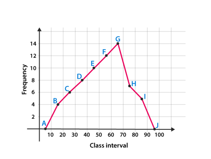
Draw the frequency polygon for the following data

Mark the class interval along x-axis and frequencies along the y-axis.

Let assume that class interval 0-10 with frequency zero and 90-100 with frequency zero.

Now calculate the midpoint of the class interval.

Using the midpoint and the frequency value from the above table, plot the points A (5, 0), B (15, 4), C (25, 6), D (35, 8), E (45, 10), F (55, 12), G (65, 14), H (75, 7), I (85, 5) and J (95, 0).

To obtain the frequency polygon ABCDEFGHIJ, draw the line segments AB, BC, CD, DE, EF, FG, GH, HI, IJ, and connect all the points.

Frequently Asked Questions

What are the different types of graphical representation.

Some of the various types of graphical representation include:

• Line Graphs
• Frequency Table
• Circle Graph, etc.

Read More:  Types of Graphs

What are the Advantages of Graphical Method?

Some of the advantages of graphical representation are:

• It makes data more easily understandable.
• It saves time.
• It makes the comparison of data more efficient.

Leave a Comment Cancel reply

Your Mobile number and Email id will not be published. Required fields are marked *

Request OTP on Voice Call

Post My Comment

Very useful for understand the basic concepts in simple and easy way. Its very useful to all students whether they are school students or college sudents

Thanks very much for the information

• Share Share

Register with BYJU'S & Download Free PDFs

Register with byju's & watch live videos.

Graphical summaries of data #

Many powerful approaches to data analysis communicate their findings via graphs. These are an important counterpart to data analysis approaches that communicate their findings via numbers or tabless.

Here we will illustrate some of the most common approaches for graphical data analysis. Throughout this discussion, it is important to remember that graphical data analysis methods are subject to the same principles as non-graphical methods. A graph can be either informative or misleading, just like any other type of statistical result. To understand whether a graph is informative, we should consider the following:

Every graph should provide insight into the specific research question that is the overall goal of the data analysis.

The graph is constructed using a sample of data, but the purpose of the graph is to learn about the population that the sample represents.

What statistical principal or concept is the graph based on?

What are the theoretical properties of any numerical summaries that are shown in the graph?

Almost every statistical graphic conveys a statistical concept that can be defined in a non-graphical manner. Graphs may show associations, location, dispersion, tails, conditioning, or almost any other statistical feature of the data or population. Graphs make it easier for the viewer to digest such information, but when interpreting a graph it is always important to keep in mind the specific statistical concept on which the graph is based.

Statistical graphics have an aesthetic dimension that is usually not evident when presenting findings through, say, tables. Our goal here is to focus on the content of graphs, not their aesthetic properties. Very crude graphs that have deep content are much more informative than beautiful graphs that convey only superficial content. In recent years, the field of infographics has grown rapidly. There is no sharp line dividing infographics from statistical graphs, however in general, the former tend to convey relatively simple insights in an aesthetically engaging way, while the latter aim to convey deeper and more subtle insight, with less focus on presentation.

Challenges and limitations of graphs #

One of the main challenges in statistical graphics is to fit the greatest amount of useful information into a single graph, while allowing the graph to remain interpretable. More complex graphs can suffer from overplotting , in which the plot elements are so crowded on the page that they fall on top of each other. This can limit the legibility of plots formed from large datasets unless a great deal of preliminary summarization of the data is performed.

Another challenge that arises in graphing complex datasets is that most graphs are two-dimensional, so that they can be viewed on a screen (or printed on paper). Some graphing techniques extend to three dimensions, but many datasets have a natural dimensionality that is much greater than 2 or 3. A few methods for graphing work around this, but require more effort from the person viewing the graph.

Boxplots are a graphical representation of the distribution of a single quantitative variable. A boxplot is based on a set of quantiles calculated using a sample of data. Below is an example of a single boxplot, drawn horizontally, showing the distribution of income values based on a sample of 100 individuals.

The “box” in a boxplot (shaded blue above) spans from the 25th to the 75th percentiles of the data, with an additional line drawn cross-wise through the box at the median. “Whiskers” extend from either end of the box, and are intended to cover the range of the data, excluding “outliers”.

The concept of an outlier is extremely problematic and no generically useful definition of outliers has been proposed. For the purpose of drawing a boxplot, the most common convention is to plot the upper (right-most) whisker at the 75th percentile plus 1.5 times the IQR, or to the greatest data value less than this quantity. Analogously, the lower (left-most) whisker is drawn at the 25th percentile minus 1.5 times the IQR, or to the least data value greater than this quantity. Finally, individual points sometimes called “fliers” are drawn corresponding to any value that falls outside the range spanned by the whiskers. A single box-plot, as above, is often drawn horizontally, but may also be drawn vertically.

There are many alternative ways of defining the locations of the whiskers in a boxplot. The approach described above is most common, and is chosen so that with “light tailed” distributions, well under 1% of the data will fall outside of of the whiskers.

The boxplot above shows a right-skewed distribution. This is evident because the upper whisker is further from the box than the lower whisker. Also, within the box, the median is closer to the lower side of the box than to the upper side of the box. Overall, the lower quantiles are more compressed, and the upper quantiles are more spread out, which is a feature of right-skewed distributions.

Side-by-side boxplots #

Boxplots are commonly used to compare distributions. A “side-by-side” or “grouped” boxplot is a collection of boxplots drawn for different subsets of data, plotted on the same axes. These subsets usually result from a stratification of the data, according to some stratifying factor that partially accounts for the heterogeneity within the population of interest. For example, below we consider boxplots showing the distribution of income, stratified by sex.

Histograms #

A histogram is a very familiar way to visualize quantitative data. A histogram is constructed by breaking the range of the values into bins and counting the number (or proportion) of observations that fall into each bin. The shape of a histogram shows visually how likely we are to observe data value in each part of the range. We are more likely to observe values where the histogram bars are higher, and less likely to observe values where the histogram bars are lower.

Histograms closely resemble “bar charts”, but with the added statistical aspect that the goal is to capture the density at each possible point in the population. “Density” is a measure of how commonly we observe data “near”, rather than “at” a point. For example, the density of household incomes at 45,000 USD would not be the exact number or frequency of households with this income. Instead, it reflects the frequency of households that have an income near 45,000 USD.

A histogram can be used to assess almost any property of a distribution. The common measures of location and dispersion can be judged from visual inspection of the histogram. As always, we should remember that features of the histogram may not always reflect features of the population from which the data were sampled. For example, a histogram may show two modes (i.e. is bimodal ) even when the underlying distribution only has one mode (i.e. is unimodal ). Moreover, the number of modes in a histogram can change as the bin width is varied.

Histograms are easy to communicate about, but may not be effective when working with small samples, where they can accentuate non-generalizable features of the sample (i.e. characteristics of the sample that are not present in the population). This is reflected in the following mathematical fact. For many statistics, if we wish to reduce the error relative to the population value of the statistic by a factor of two, we need to increase the sample size by a factor of four. In the case where we are aiming to estimate a density, in order to reduce the error by a factor of two, we need to increase the sample size by a factor of eight.

With a sufficiently large collection of representative data, the histogram should closely match the population’s probability density function (PDF). The PDF is usually a smooth curve, rather than a series of steps as in a histogram. This fact inspired the development of a modified version of a histogram that presents us with a smooth curve instead of a series of steps. This technique is called kernel density estimation ( KDE ). It produces graphs such as shown below.

Kernel density estimates may provide a somewhat more accurate estimation of the underlying density function compared to a histogram. But like a histogram, they can be unstable and produce artifacts. For example, the KDE above shows positive density for negative income values, even though all of the income values used to fit the KDE were positive (in some cases, income can take a negative value, but in this case no such values were present). More advanced KDE methods not used here can mitigate this issue.

One advantage of using a KDE rather than a histogram is that it is easier to overlay multiple KDEs on the same axes for comparison without too much overplotting. This might allow us to compare, say, the distributions of female and male incomes as follows.

Quantile plots #

A quantile plot is a plot of the pairs \((p, q_p)\) , where \(q_p\) is the p’th quantile of a collection of quantitative values. Since \(p\) can be any real number between 0 and 1, the graph of these pairs constitutes a function. By construction, this must be a non-decreasing function. A quantile plot contains essentially the same information as a histogram, but is represented in a very different way. Note that unlike the histogram, for which the bin width is a parameter that must be selected, there is no such parameter in the quantile plot. Arguably, the quantile plot is a more stable and informative summary of a sample, especially if the sample size is moderate. However most people are more comfortable interpreting histograms than quantile functions.

As an example, the following plot shows simulated systolic blood pressure values for a sample of females and a sample of males. In this case, at every probability point \(p\) , the blood pressure quantile for males is greater than the blood pressure quantile for females, indicating that male blood pressure is “stochastically greater” than female blood pressure.

Below is another example that shows two quantile functions, but in this case the quantile functions cross. As a result, there is no “stochastic ordering” between the data for females and for males. Also note that the quantile curve for females is steeper than the curve for males, indicating that the female blood pressure values are more dispersed than those for the males.

Quantile-quantile plots #

A quantile-quantile plot , or QQ plot , is a plot based on quantiles that is used to compare two distributions. Recall that a quantile plot plots the pairs \((p, q_p)\) for one sample. A QQ plot plots the pairs \((q^{(1)}_p, q^{(2)}_p)\) , where \(q^{(1)}_p\) are the quantiles for the first sample, and \(q^{(2)}_p\) are the quantiles for the second sample. In a QQ-plot, the value of p is “implicit” – each point on the graph corresponds to a specific value of p, but you cannot see what this value is by inspecting the graph.

As an example, suppose we are comparing the number of minutes of sleep during one night for teenagers and adults. This might give us the following QQ-plot:

The above QQ-plot shows us that teenagers tend to sleep longer than adults, and this is especially true at the upper end of the range. The QQ-plot approximately passes through the point (600, 800), meaning that for some probability p, 600 is the p’th quantile for adults and 800 is the p’th quantile for teenagers.

The slope of the curve in the QQ-plot reflects the relative levels of dispersion in the two distributions being compared. Since the slope of the curve in the above QQ-plot is greater than that of the diagonal reference line, it follows that the values plotted on the vertical axis (teenager’s values) are more dispersed than the values plotted on the horizontal axis (adult’s values).

An important property of a QQ-plot is that if the plot shows a linear relationship between the quantiles, then the two distributions are related via a location/scale transformation . That is, there is a linear function \(a + bx\) that maps one distribution to the other. In the example above, there is a substantial amount of curvature in the graph, so it does not seem to be the case that the sleep durations for adults and teenagers are related via a location/scale transformation.

Dot plots #

Dot plots display quantitative data that are stratified into groups. One axis of the plot is used to display the quantitative measure, and the other axis is used to separate the results for different groups. A series of parallel “guide lines” are used to show which points belong to each group. Dot plots are often used to display a collection of numerical summary statistics in visual form. Sometimes people say that dot plots are used to “convert tables into graphs”. Due to overplotting, dot plots are less commonly used to show raw data. The example below shows how dot plots can be used to display the median age stratified by sex, for people living in each of eleven countries.

The plot above shows that the median age for females is greater than the median age for males in every country. This is mainly due to females having longer life expectancies than males. We also see that some countries have much lower median ages for both sexes compared to other countries. Countries that have recently had high birth rates, such as Ethiopia and Nigeria, tend to have much lower median ages than countries with lower birth rates, such as Japan.

Scatterplots #

A scatterplot is a very widely-used method for visualizing bivariate data. They have many uses, but the most relevant for us is to plot the joint (empirical) distribution of two quantitative values. As an example, suppose that we observe paired data values giving the annual minimum and annual maximum temperature at a location. We could view these data with a scatterplot, placing, say, the minimum temperature value on the horizontal (x) axis, and the maximum temperature value on the vertical (y) axis. The number of points is the sample size, here being the number of locations for which temperature data are available. A possible graph of this type is shown below.

Several characteristics of the relationship between minimum and maximum temperature are evident from the plot above. The maximum temperature at each location is at least as large as the minimum temperature. There is a positive association in which locations with a lower minimum temperature tend to have a lower maximum temperature compared to places with a higher maximum temperature, but there is a lot of scatter around this trend. Warmer places tend to have a smaller range between their minimum and maximum temperatures. Concretely, locations on the equator and at low elevation, such as Singapore, have relatively constant temperature throughout the year. Locations near the center of large continents, like Winnipeg, Canada, can have extremely cold winters and also rather hot summers. Coastal regions that are far from the equator, such as Dublin, Ireland, have mild winters and cool summers.

To aid in interpreting a scatterplot, it is useful to plot a smooth curve that runs through the center of the data. This is called scatterplot smoothing , and can be accomplished with several algorithms, one of which is known as lowess . The population analogue of a scatterplot smooth is the conditional mean , or conditional expectation , denoted \(E[Y|X=x]\) , for the conditional mean of \(Y\) given \(X\) . The conditional mean is a function of \(x\) , and can be evaluated at any point \(x\) in the domain of \(X\) . The conditional mean is (roughly speaking), the average of all values of \(Y\) whose corresponding value of \(X\) is near \(x\) .

The plot below adds the estimated conditional mean (orange curve) to the scatterplot of temperature data discussed above. The conditional mean curve is increasing, showing that, as noted above, a location with lower annual minimum temperature tends on average to have a lower annual maximum temperature (relative to other locations).

Time series plots #

Some data have a serial structure, meaning that the values are observed with an ordering. Very often, such observations are made over time, which gives us time series or longitudinal data. Sometimes we observe a single time series over a long period of time, such as the value of a commodity in a market recorded every day over many years. Other times, we observe many short time series recorded irregularly. We may plot these time series together, leading to what is sometimes called a “spaghetti plot”. For example, in a study of human growth, we may observe measurements of the body weight of research subjects at various ages, giving us the spaghetti plot below:

Parallel coordinate plots #

Scatterplots in the plane are limited to two dimensions. Various techniques have been developed to overcome this limitation, one of which is the parallel coordinate plot . A parallel coordinate plot places the coordinate axes for the multiple dimensions as parallel lines, rather than as perpendicular lines. Using parallel lines means that data for far more than two or three variables can be placed on a single page.

Below is an example of a parallel coordinates plot, showing four attributes of a set of ten countries. A scatterplot of these points would live in four-dimensional space, which is quite challenging to visualize directly. Note that the attributes are converted to Z-scores, which is common in a parallel coordinates plot when the variables being plotted fall in very different ranges. The plot shows us that the life expectancies for females and for males are quite similar – the country with the highest life expectancy for females also has the highest life expectancy for males, and the country with the lowest life expectancy for females also has the lowest life expectancy for males. There is also a substantial positive relationship between the economic status of a country, as measured by its gross domestic product (GDP) and life expectancy. However no relationship is evident between GDP and population, or between either of the life expectancy variables and population.

Mosaic plots #

The graphs above primarily use quantitative data. A mosaic plot is a plot that is used with nominal data. Specifically mosaic plots are used when the units of analysis are cross-classified according to two nominal factors. In the example below, people with cancer are cross-classified by their biological sex, and by the type of cancer that they have:

The width of each box in the mosaic plot corresponds to the relative overall prevalence of the corresponding cancer type. The heights of the boxes correspond to the sex-specific prevalences. Based on this graph, we see that digestive, lung, and breast cancers are much more common than, say, oral and endocrine cancers. The mosaic plot also shows us that while breast and endocrine cancers are more common in females, the other cancer types are more common in males.

An important property of a mosaic plot is that the area of each box is proportional to the number of units that fall into the box. Thus, we can see that the area of the female breast cancer box is larger than the the combined areas of the female and male lung cancer boxes. Thus, there are more cases of breast cancer in females than the combined cases of lung cancer for both sexes.

• Business Essentials
• Leadership & Management
• Credential of Leadership, Impact, and Management in Business (CLIMB)
• Entrepreneurship & Innovation
• Digital Transformation
• Finance & Accounting
• Business in Society
• For Organizations
• Support Portal
• Media Coverage
• Founding Donors
• Leadership Team

• Harvard Business School →
• HBS Online →
• Business Insights →

Business Insights

Harvard Business School Online's Business Insights Blog provides the career insights you need to achieve your goals and gain confidence in your business skills.

• Career Development
• Communication
• Decision-Making
• Earning Your MBA
• Negotiation
• News & Events
• Productivity
• Staff Spotlight
• Student Profiles
• Work-Life Balance
• AI Essentials for Business
• Alternative Investments
• Business Analytics
• Business Strategy
• Business and Climate Change
• Design Thinking and Innovation
• Digital Marketing Strategy
• Disruptive Strategy
• Economics for Managers
• Entrepreneurship Essentials
• Financial Accounting
• Global Business
• Launching Tech Ventures
• Leadership Principles
• Leadership, Ethics, and Corporate Accountability
• Leading with Finance
• Management Essentials
• Negotiation Mastery
• Organizational Leadership
• Power and Influence for Positive Impact
• Strategy Execution
• Sustainable Business Strategy
• Sustainable Investing
• Winning with Digital Platforms

17 Data Visualization Techniques All Professionals Should Know

• 17 Sep 2019

There’s a growing demand for business analytics and data expertise in the workforce. But you don’t need to be a professional analyst to benefit from data-related skills.

Becoming skilled at common data visualization techniques can help you reap the rewards of data-driven decision-making , including increased confidence and potential cost savings. Learning how to effectively visualize data could be the first step toward using data analytics and data science to your advantage to add value to your organization.

Several data visualization techniques can help you become more effective in your role. Here are 17 essential data visualization techniques all professionals should know, as well as tips to help you effectively present your data.

Access your free e-book today.

What Is Data Visualization?

Data visualization is the process of creating graphical representations of information. This process helps the presenter communicate data in a way that’s easy for the viewer to interpret and draw conclusions.

There are many different techniques and tools you can leverage to visualize data, so you want to know which ones to use and when. Here are some of the most important data visualization techniques all professionals should know.

Data Visualization Techniques

The type of data visualization technique you leverage will vary based on the type of data you’re working with, in addition to the story you’re telling with your data .

Here are some important data visualization techniques to know:

• Gantt Chart
• Box and Whisker Plot
• Waterfall Chart
• Scatter Plot
• Pictogram Chart
• Highlight Table
• Bullet Graph
• Choropleth Map
• Network Diagram
• Correlation Matrices

1. Pie Chart

Pie charts are one of the most common and basic data visualization techniques, used across a wide range of applications. Pie charts are ideal for illustrating proportions, or part-to-whole comparisons.

Because pie charts are relatively simple and easy to read, they’re best suited for audiences who might be unfamiliar with the information or are only interested in the key takeaways. For viewers who require a more thorough explanation of the data, pie charts fall short in their ability to display complex information.

2. Bar Chart

The classic bar chart , or bar graph, is another common and easy-to-use method of data visualization. In this type of visualization, one axis of the chart shows the categories being compared, and the other, a measured value. The length of the bar indicates how each group measures according to the value.

One drawback is that labeling and clarity can become problematic when there are too many categories included. Like pie charts, they can also be too simple for more complex data sets.

3. Histogram

Unlike bar charts, histograms illustrate the distribution of data over a continuous interval or defined period. These visualizations are helpful in identifying where values are concentrated, as well as where there are gaps or unusual values.

Histograms are especially useful for showing the frequency of a particular occurrence. For instance, if you’d like to show how many clicks your website received each day over the last week, you can use a histogram. From this visualization, you can quickly determine which days your website saw the greatest and fewest number of clicks.

4. Gantt Chart

Gantt charts are particularly common in project management, as they’re useful in illustrating a project timeline or progression of tasks. In this type of chart, tasks to be performed are listed on the vertical axis and time intervals on the horizontal axis. Horizontal bars in the body of the chart represent the duration of each activity.

Utilizing Gantt charts to display timelines can be incredibly helpful, and enable team members to keep track of every aspect of a project. Even if you’re not a project management professional, familiarizing yourself with Gantt charts can help you stay organized.

5. Heat Map

A heat map is a type of visualization used to show differences in data through variations in color. These charts use color to communicate values in a way that makes it easy for the viewer to quickly identify trends. Having a clear legend is necessary in order for a user to successfully read and interpret a heatmap.

There are many possible applications of heat maps. For example, if you want to analyze which time of day a retail store makes the most sales, you can use a heat map that shows the day of the week on the vertical axis and time of day on the horizontal axis. Then, by shading in the matrix with colors that correspond to the number of sales at each time of day, you can identify trends in the data that allow you to determine the exact times your store experiences the most sales.

6. A Box and Whisker Plot

A box and whisker plot , or box plot, provides a visual summary of data through its quartiles. First, a box is drawn from the first quartile to the third of the data set. A line within the box represents the median. “Whiskers,” or lines, are then drawn extending from the box to the minimum (lower extreme) and maximum (upper extreme). Outliers are represented by individual points that are in-line with the whiskers.

This type of chart is helpful in quickly identifying whether or not the data is symmetrical or skewed, as well as providing a visual summary of the data set that can be easily interpreted.

7. Waterfall Chart

A waterfall chart is a visual representation that illustrates how a value changes as it’s influenced by different factors, such as time. The main goal of this chart is to show the viewer how a value has grown or declined over a defined period. For example, waterfall charts are popular for showing spending or earnings over time.

8. Area Chart

An area chart , or area graph, is a variation on a basic line graph in which the area underneath the line is shaded to represent the total value of each data point. When several data series must be compared on the same graph, stacked area charts are used.

This method of data visualization is useful for showing changes in one or more quantities over time, as well as showing how each quantity combines to make up the whole. Stacked area charts are effective in showing part-to-whole comparisons.

9. Scatter Plot

Another technique commonly used to display data is a scatter plot . A scatter plot displays data for two variables as represented by points plotted against the horizontal and vertical axis. This type of data visualization is useful in illustrating the relationships that exist between variables and can be used to identify trends or correlations in data.

Scatter plots are most effective for fairly large data sets, since it’s often easier to identify trends when there are more data points present. Additionally, the closer the data points are grouped together, the stronger the correlation or trend tends to be.

10. Pictogram Chart

Pictogram charts , or pictograph charts, are particularly useful for presenting simple data in a more visual and engaging way. These charts use icons to visualize data, with each icon representing a different value or category. For example, data about time might be represented by icons of clocks or watches. Each icon can correspond to either a single unit or a set number of units (for example, each icon represents 100 units).

In addition to making the data more engaging, pictogram charts are helpful in situations where language or cultural differences might be a barrier to the audience’s understanding of the data.

11. Timeline

Timelines are the most effective way to visualize a sequence of events in chronological order. They’re typically linear, with key events outlined along the axis. Timelines are used to communicate time-related information and display historical data.

Timelines allow you to highlight the most important events that occurred, or need to occur in the future, and make it easy for the viewer to identify any patterns appearing within the selected time period. While timelines are often relatively simple linear visualizations, they can be made more visually appealing by adding images, colors, fonts, and decorative shapes.

12. Highlight Table

A highlight table is a more engaging alternative to traditional tables. By highlighting cells in the table with color, you can make it easier for viewers to quickly spot trends and patterns in the data. These visualizations are useful for comparing categorical data.

Depending on the data visualization tool you’re using, you may be able to add conditional formatting rules to the table that automatically color cells that meet specified conditions. For instance, when using a highlight table to visualize a company’s sales data, you may color cells red if the sales data is below the goal, or green if sales were above the goal. Unlike a heat map, the colors in a highlight table are discrete and represent a single meaning or value.

13. Bullet Graph

A bullet graph is a variation of a bar graph that can act as an alternative to dashboard gauges to represent performance data. The main use for a bullet graph is to inform the viewer of how a business is performing in comparison to benchmarks that are in place for key business metrics.

In a bullet graph, the darker horizontal bar in the middle of the chart represents the actual value, while the vertical line represents a comparative value, or target. If the horizontal bar passes the vertical line, the target for that metric has been surpassed. Additionally, the segmented colored sections behind the horizontal bar represent range scores, such as “poor,” “fair,” or “good.”

14. Choropleth Maps

A choropleth map uses color, shading, and other patterns to visualize numerical values across geographic regions. These visualizations use a progression of color (or shading) on a spectrum to distinguish high values from low.

Choropleth maps allow viewers to see how a variable changes from one region to the next. A potential downside to this type of visualization is that the exact numerical values aren’t easily accessible because the colors represent a range of values. Some data visualization tools, however, allow you to add interactivity to your map so the exact values are accessible.

15. Word Cloud

A word cloud , or tag cloud, is a visual representation of text data in which the size of the word is proportional to its frequency. The more often a specific word appears in a dataset, the larger it appears in the visualization. In addition to size, words often appear bolder or follow a specific color scheme depending on their frequency.

Word clouds are often used on websites and blogs to identify significant keywords and compare differences in textual data between two sources. They are also useful when analyzing qualitative datasets, such as the specific words consumers used to describe a product.

16. Network Diagram

Network diagrams are a type of data visualization that represent relationships between qualitative data points. These visualizations are composed of nodes and links, also called edges. Nodes are singular data points that are connected to other nodes through edges, which show the relationship between multiple nodes.

There are many use cases for network diagrams, including depicting social networks, highlighting the relationships between employees at an organization, or visualizing product sales across geographic regions.

17. Correlation Matrix

A correlation matrix is a table that shows correlation coefficients between variables. Each cell represents the relationship between two variables, and a color scale is used to communicate whether the variables are correlated and to what extent.

Correlation matrices are useful to summarize and find patterns in large data sets. In business, a correlation matrix might be used to analyze how different data points about a specific product might be related, such as price, advertising spend, launch date, etc.

Other Data Visualization Options

While the examples listed above are some of the most commonly used techniques, there are many other ways you can visualize data to become a more effective communicator. Some other data visualization options include:

• Bubble clouds
• Circle views
• Dendrograms
• Dot distribution maps
• Open-high-low-close charts
• Polar areas
• Radial trees
• Ring Charts
• Sankey diagram
• Span charts
• Streamgraphs
• Wedge stack graphs
• Violin plots

Tips For Creating Effective Visualizations

Creating effective data visualizations requires more than just knowing how to choose the best technique for your needs. There are several considerations you should take into account to maximize your effectiveness when it comes to presenting data.

Related : What to Keep in Mind When Creating Data Visualizations in Excel

One of the most important steps is to evaluate your audience. For example, if you’re presenting financial data to a team that works in an unrelated department, you’ll want to choose a fairly simple illustration. On the other hand, if you’re presenting financial data to a team of finance experts, it’s likely you can safely include more complex information.

Another helpful tip is to avoid unnecessary distractions. Although visual elements like animation can be a great way to add interest, they can also distract from the key points the illustration is trying to convey and hinder the viewer’s ability to quickly understand the information.

Finally, be mindful of the colors you utilize, as well as your overall design. While it’s important that your graphs or charts are visually appealing, there are more practical reasons you might choose one color palette over another. For instance, using low contrast colors can make it difficult for your audience to discern differences between data points. Using colors that are too bold, however, can make the illustration overwhelming or distracting for the viewer.

Related : Bad Data Visualization: 5 Examples of Misleading Data

Visuals to Interpret and Share Information

No matter your role or title within an organization, data visualization is a skill that’s important for all professionals. Being able to effectively present complex data through easy-to-understand visual representations is invaluable when it comes to communicating information with members both inside and outside your business.

There’s no shortage in how data visualization can be applied in the real world. Data is playing an increasingly important role in the marketplace today, and data literacy is the first step in understanding how analytics can be used in business.

Are you interested in improving your analytical skills? Learn more about Business Analytics , our eight-week online course that can help you use data to generate insights and tackle business decisions.

This post was updated on January 20, 2022. It was originally published on September 17, 2019.

About the Author

• both data sets are the same size, and
• each data point in one data set is matched with exactly one point from the other set.

As an Amazon Associate we earn from qualifying purchases.

This book may not be used in the training of large language models or otherwise be ingested into large language models or generative AI offerings without OpenStax's permission.

Want to cite, share, or modify this book? This book uses the Creative Commons Attribution License and you must attribute OpenStax.

Access for free at https://openstax.org/books/introductory-statistics/pages/1-introduction

• Authors: Barbara Illowsky, Susan Dean
• Publisher/website: OpenStax
• Book title: Introductory Statistics
• Publication date: Sep 19, 2013
• Location: Houston, Texas
• Book URL: https://openstax.org/books/introductory-statistics/pages/1-introduction
• Section URL: https://openstax.org/books/introductory-statistics/pages/2-key-terms

© Jun 23, 2022 OpenStax. Textbook content produced by OpenStax is licensed under a Creative Commons Attribution License . The OpenStax name, OpenStax logo, OpenStax book covers, OpenStax CNX name, and OpenStax CNX logo are not subject to the Creative Commons license and may not be reproduced without the prior and express written consent of Rice University.

16 Best Types of Charts and Graphs for Data Visualization [+ Guide]

Published: June 08, 2023

There are more type of charts and graphs than ever before because there's more data. In fact, the volume of data in 2025 will be almost double the data we create, capture, copy, and consume today.

This makes data visualization essential for businesses. Different types of graphs and charts can help you:

• Motivate your team to take action.
• Impress stakeholders with goal progress.
• Show your audience what you value as a business.

Data visualization builds trust and can organize diverse teams around new initiatives. Let's talk about the types of graphs and charts that you can use to grow your business.

Free Excel Graph Templates

Tired of struggling with spreadsheets? These free Microsoft Excel Graph Generator Templates can help.

• Simple, customizable graph designs.
• Data visualization tips & instructions.
• Templates for two, three, four, and five-variable graph templates.

You're all set!

Click this link to access this resource at any time.

Different Types of Graphs for Data Visualization

1. bar graph.

A bar graph should be used to avoid clutter when one data label is long or if you have more than 10 items to compare.

Best Use Cases for These Types of Graphs

Bar graphs can help you compare data between different groups or to track changes over time. Bar graphs are most useful when there are big changes or to show how one group compares against other groups.

The example above compares the number of customers by business role. It makes it easy to see that there is more than twice the number of customers per role for individual contributors than any other group.

A bar graph also makes it easy to see which group of data is highest or most common.

For example, at the start of the pandemic, online businesses saw a big jump in traffic. So, if you want to look at monthly traffic for an online business, a bar graph would make it easy to see that jump.

Other use cases for bar graphs include:

• Product comparisons.
• Product usage.
• Category comparisons.
• Marketing traffic by month or year.
• Marketing conversions.

Design Best Practices for Bar Graphs

• Use consistent colors throughout the chart, selecting accent colors to highlight meaningful data points or changes over time.
• Use horizontal labels to improve readability.
• Start the y-axis at 0 to appropriately reflect the values in your graph.

2. Line Graph

A line graph reveals trends or progress over time, and you can use it to show many different categories of data. You should use it when you chart a continuous data set.

Line graphs help users track changes over short and long periods. Because of this, these types of graphs are good for seeing small changes.

Line graphs can help you compare changes for more than one group over the same period. They're also helpful for measuring how different groups relate to each other.

A business might use this graph to compare sales rates for different products or services over time.

These charts are also helpful for measuring service channel performance. For example, a line graph that tracks how many chats or emails your team responds to per month.

Design Best Practices for Line Graphs

• Use solid lines only.
• Don't plot more than four lines to avoid visual distractions.
• Use the right height so the lines take up roughly 2/3 of the y-axis' height.

3. Bullet Graph

A bullet graph reveals progress towards a goal, compares this to another measure, and provides context in the form of a rating or performance.

In the example above, the bullet graph shows the number of new customers against a set customer goal. Bullet graphs are great for comparing performance against goals like this.

These types of graphs can also help teams assess possible roadblocks because you can analyze data in a tight visual display.

For example, you could create a series of bullet graphs measuring performance against benchmarks or use a single bullet graph to visualize these KPIs against their goals:

• Customer satisfaction.
• Average order size.
• New customers.

Seeing this data at a glance and alongside each other can help teams make quick decisions.

Bullet graphs are one of the best ways to display year-over-year data analysis. You can also use bullet graphs to visualize:

• Customer satisfaction scores.
• Customer shopping habits.
• Social media usage by platform.

Design Best Practices for Bullet Graphs

• Use contrasting colors to highlight how the data is progressing.
• Use one color in different shades to gauge progress.

Different Types of Charts for Data Visualization

To better understand these chart types and how you can use them, here's an overview of each:

1. Column Chart

Use a column chart to show a comparison among different items or to show a comparison of items over time. You could use this format to see the revenue per landing page or customers by close date.

Best Use Cases for This Type of Chart

You can use both column charts and bar graphs to display changes in data, but column charts are best for negative data. The main difference, of course, is that column charts show information vertically while bar graphs show data horizontally.

For example, warehouses often track the number of accidents on the shop floor. When the number of incidents falls below the monthly average, a column chart can make that change easier to see in a presentation.

In the example above, this column chart measures the number of customers by close date. Column charts make it easy to see data changes over a period of time. This means that they have many use cases, including:

• Customer survey data, like showing how many customers prefer a specific product or how much a customer uses a product each day.
• Sales volume, like showing which services are the top sellers each month or the number of sales per week.
• Profit and loss, showing where business investments are growing or falling.

Design Best Practices for Column Charts

2. dual-axis chart.

A dual-axis chart allows you to plot data using two y-axes and a shared x-axis. It has three data sets. One is a continuous data set, and the other is better suited to grouping by category. Use this chart to visualize a correlation or the lack thereof between these three data sets.

A dual-axis chart makes it easy to see relationships between different data sets. They can also help with comparing trends.

For example, the chart above shows how many new customers this company brings in each month. It also shows how much revenue those customers are bringing the company.

This makes it simple to see the connection between the number of customers and increased revenue.

You can use dual-axis charts to compare:

• Price and volume of your products.
• Revenue and units sold.
• Sales and profit margin.
• Individual sales performance.

Design Best Practices for Dual-Axis Charts

• Use the y-axis on the left side for the primary variable because brains naturally look left first.
• Use different graphing styles to illustrate the two data sets, as illustrated above.
• Choose contrasting colors for the two data sets.

3. Area Chart

An area chart is basically a line chart, but the space between the x-axis and the line is filled with a color or pattern. It is useful for showing part-to-whole relations, like showing individual sales reps’ contributions to total sales for a year. It helps you analyze both overall and individual trend information.

Best Use Cases for These Types of Charts

Area charts help show changes over time. They work best for big differences between data sets and help visualize big trends.

For example, the chart above shows users by creation date and life cycle stage.

A line chart could show more subscribers than marketing qualified leads. But this area chart emphasizes how much bigger the number of subscribers is than any other group.

These charts make the size of a group and how groups relate to each other more visually important than data changes over time.

Area graphs can help your business to:

• Visualize which product categories or products within a category are most popular.
• Show key performance indicator (KPI) goals vs. outcomes.
• Spot and analyze industry trends.

Design Best Practices for Area Charts

• Use transparent colors so information isn't obscured in the background.
• Don't display more than four categories to avoid clutter.
• Organize highly variable data at the top of the chart to make it easy to read.

4. Stacked Bar Chart

Use this chart to compare many different items and show the composition of each item you’re comparing.

These graphs are helpful when a group starts in one column and moves to another over time.

For example, the difference between a marketing qualified lead (MQL) and a sales qualified lead (SQL) is sometimes hard to see. The chart above helps stakeholders see these two lead types from a single point of view — when a lead changes from MQL to SQL.

Stacked bar charts are excellent for marketing. They make it simple to add a lot of data on a single chart or to make a point with limited space.

These graphs can show multiple takeaways, so they're also super for quarterly meetings when you have a lot to say but not a lot of time to say it.

Stacked bar charts are also a smart option for planning or strategy meetings. This is because these charts can show a lot of information at once, but they also make it easy to focus on one stack at a time or move data as needed.

You can also use these charts to:

• Show the frequency of survey responses.
• Identify outliers in historical data.
• Compare a part of a strategy to its performance as a whole.

Design Best Practices for Stacked Bar Graphs

• Best used to illustrate part-to-whole relationships.
• Use contrasting colors for greater clarity.
• Make the chart scale large enough to view group sizes in relation to one another.

5. Mekko Chart

Also known as a Marimekko chart, this type of graph can compare values, measure each one's composition, and show data distribution across each one.

It's similar to a stacked bar, except the Mekko's x-axis can capture another dimension of your values — instead of time progression, like column charts often do. In the graphic below, the x-axis compares the cities to one another.

Image Source

You can use a Mekko chart to show growth, market share, or competitor analysis.

For example, the Mekko chart above shows the market share of asset managers grouped by location and the value of their assets. This chart clarifies which firms manage the most assets in different areas.

It's also easy to see which asset managers are the largest and how they relate to each other.

Mekko charts can seem more complex than other types of charts and graphs, so it's best to use these in situations where you want to emphasize scale or differences between groups of data.

Other use cases for Mekko charts include:

• Detailed profit and loss statements.
• Revenue by brand and region.
• Product profitability.
• Share of voice by industry or niche.

Design Best Practices for Mekko Charts

• Vary your bar heights if the portion size is an important point of comparison.
• Don't include too many composite values within each bar. Consider reevaluating your presentation if you have a lot of data.
• Order your bars from left to right in such a way that exposes a relevant trend or message.

6. Pie Chart

A pie chart shows a static number and how categories represent part of a whole — the composition of something. A pie chart represents numbers in percentages, and the total sum of all segments needs to equal 100%.

The image above shows another example of customers by role in the company.

The bar graph example shows you that there are more individual contributors than any other role. But this pie chart makes it clear that they make up over 50% of customer roles.

Pie charts make it easy to see a section in relation to the whole, so they are good for showing:

• Customer personas in relation to all customers.
• Revenue from your most popular products or product types in relation to all product sales.
• Percent of total profit from different store locations.

Design Best Practices for Pie Charts

• Don't illustrate too many categories to ensure differentiation between slices.
• Ensure that the slice values add up to 100%.
• Order slices according to their size.

7. Scatter Plot Chart

A scatter plot or scattergram chart will show the relationship between two different variables or reveal distribution trends.

Use this chart when there are many different data points, and you want to highlight similarities in the data set. This is useful when looking for outliers or understanding your data's distribution.

Scatter plots are helpful in situations where you have too much data to see a pattern quickly. They are best when you use them to show relationships between two large data sets.

In the example above, this chart shows how customer happiness relates to the time it takes for them to get a response.

This type of graph makes it easy to compare two data sets. Use cases might include:

• Employment and manufacturing output.
• Retail sales and inflation.
• Visitor numbers and outdoor temperature.
• Sales growth and tax laws.

Try to choose two data sets that already have a positive or negative relationship. That said, this type of graph can also make it easier to see data that falls outside of normal patterns.

Design Best Practices for Scatter Plots

• Include more variables, like different sizes, to incorporate more data.
• Start the y-axis at 0 to represent data accurately.
• If you use trend lines, only use a maximum of two to make your plot easy to understand.

8. Bubble Chart

A bubble chart is similar to a scatter plot in that it can show distribution or relationship. There is a third data set shown by the size of the bubble or circle.

In the example above, the number of hours spent online isn't just compared to the user's age, as it would be on a scatter plot chart.

Instead, you can also see how the gender of the user impacts time spent online.

This makes bubble charts useful for seeing the rise or fall of trends over time. It also lets you add another option when you're trying to understand relationships between different segments or categories.

For example, if you want to launch a new product, this chart could help you quickly see your new product's cost, risk, and value. This can help you focus your energies on a low-risk new product with a high potential return.

You can also use bubble charts for:

• Top sales by month and location.
• Customer satisfaction surveys.
• Store performance tracking.
• Marketing campaign reviews.

Design Best Practices for Bubble Charts

• Scale bubbles according to area, not diameter.
• Make sure labels are clear and visible.
• Use circular shapes only.

9. Waterfall Chart

Use a waterfall chart to show how an initial value changes with intermediate values — either positive or negative — and results in a final value.

Use this chart to reveal the composition of a number. An example of this would be to showcase how different departments influence overall company revenue and lead to a specific profit number.

The most common use case for a funnel chart is the marketing or sales funnel. But there are many other ways to use this versatile chart.

If you have at least four stages of sequential data, this chart can help you easily see what inputs or outputs impact the final results.

For example, a funnel chart can help you see how to improve your buyer journey or shopping cart workflow. This is because it can help pinpoint major drop-off points.

Other stellar options for these types of charts include:

• Deal pipelines.
• Conversion and retention analysis.
• Bottlenecks in manufacturing and other multi-step processes.
• Marketing campaign performance.
• Website conversion tracking.

Design Best Practices for Funnel Charts

• Scale the size of each section to accurately reflect the size of the data set.
• Use contrasting colors or one color in graduated hues, from darkest to lightest, as the size of the funnel decreases.

11. Heat Map

A heat map shows the relationship between two items and provides rating information, such as high to low or poor to excellent. This chart displays the rating information using varying colors or saturation.

Best Use Cases for Heat Maps

In the example above, the darker the shade of green shows where the majority of people agree.

With enough data, heat maps can make a viewpoint that might seem subjective more concrete. This makes it easier for a business to act on customer sentiment.

There are many uses for these types of charts. In fact, many tech companies use heat map tools to gauge user experience for apps, online tools, and website design .

Another common use for heat map graphs is location assessment. If you're trying to find the right location for your new store, these maps can give you an idea of what the area is like in ways that a visit can't communicate.

Heat maps can also help with spotting patterns, so they're good for analyzing trends that change quickly, like ad conversions. They can also help with:

• Competitor research.
• Customer sentiment.
• Sales outreach.
• Campaign impact.
• Customer demographics.

Design Best Practices for Heat Map

• Use a basic and clear map outline to avoid distracting from the data.
• Use a single color in varying shades to show changes in data.
• Avoid using multiple patterns.

12. Gantt Chart

The Gantt chart is a horizontal chart that dates back to 1917. This chart maps the different tasks completed over a period of time.

Gantt charting is one of the most essential tools for project managers. It brings all the completed and uncompleted tasks into one place and tracks the progress of each.

While the left side of the chart displays all the tasks, the right side shows the progress and schedule for each of these tasks.

This chart type allows you to:

• Break projects into tasks.
• Track the start and end of the tasks.
• Set important events, meetings, and announcements.
• Assign tasks to the team and individuals.

Download the Excel templates mentioned in the video here.

5 Questions to Ask When Deciding Which Type of Chart to Use

1. do you want to compare values.

Charts and graphs are perfect for comparing one or many value sets, and they can easily show the low and high values in the data sets. To create a comparison chart, use these types of graphs:

• Scatter plot

2. Do you want to show the composition of something?

Use this type of chart to show how individual parts make up the whole of something, like the device type used for mobile visitors to your website or total sales broken down by sales rep.

To show composition, use these charts:

• Stacked bar

3. Do you want to understand the distribution of your data?

Distribution charts help you to understand outliers, the normal tendency, and the range of information in your values.

Use these charts to show distribution:

4. Are you interested in analyzing trends in your data set?

If you want more information about how a data set performed during a specific time, there are specific chart types that do extremely well.

You should choose one of the following:

• Dual-axis line

5. Do you want to better understand the relationship between value sets?

Relationship charts can show how one variable relates to one or many different variables. You could use this to show how something positively affects, has no effect, or negatively affects another variable.

When trying to establish the relationship between things, use these charts:

Featured Resource: The Marketer's Guide to Data Visualization

Don't forget to share this post!

Related articles.

9 Great Ways to Use Data in Content Creation

Data Visualization: Tips and Examples to Inspire You

17 Data Visualization Resources You Should Bookmark

An Introduction to Data Visualization: How to Create Compelling Charts & Graphs [Ebook]

Why Data Is The Real MVP: 7 Examples of Data-Driven Storytelling by Leading Brands

How to Create an Infographic Using Poll & Survey Data [Infographic]

Data Storytelling 101: Helpful Tools for Gathering Ideas, Designing Content & More

What Great Data Visualization Looks Like: 12 Complex Concepts Made Easy

Stats Shouldn't Stand Alone: Why You Need Data Visualization to Teach and Convince

How to Harness the Power of Data to Elevate Your Content

Tired of struggling with spreadsheets? These free Microsoft Excel Graph Generator Templates can help

Marketing software that helps you drive revenue, save time and resources, and measure and optimize your investments — all on one easy-to-use platform

Geography - Representation of Geographical Data | 12th Geography : Chapter 12 : Representation of Geographical Data

Chapter: 12th geography : chapter 12 : representation of geographical data.

Representation of Geographical Data

Learning Objectives

* Identify various types of Geographical data.

* Understand various methods of drawing geographical data.

* Analyse the various methods of constructing diagram suitable for particular data.

Introduction

Economists, statisticians, and geographers make use of statistical facts and data in their respective fields. Climatic data like temperature, pressure, rainfall, etc., may be represented by diagram such as isotherms, isobars and isohyets respectively. Besides the tabular form, the data may also be presented in some graphical or diagrammatic form. Population, climatic, and Socio economic data can be represented visually for better understanding in the form of graphs, diagrams, charts and maps. Thus, geographical data needs to be scientifically visualised for appropriate cartographic communication. Therefore, cartographic presentation of geographical data is important to explore the nature of data, their pattern of variations over time and space, to analyse the data set, and to identify and classify the real world objects.

We study climatic, economic and population data in geography. The numerical data or facts when collected in a systematic manner to serve some purpose and presented in a tabulated form they are called statistics.

The diagrams representing statistical data are known as statistical diagrams. Geometrical figures such as bars, rectangles, squares, circles, cubes, sphere, etc., and curves or lines are used to represent statistical data diagrammatically. These diagrams serve the following purposes:

1. They enable us to compare figures at a glance.

2. They cast easily memorable impression on the mind.

3. They enable us to analyse the data and draw inference easily.

Related Topics

Privacy Policy , Terms and Conditions , DMCA Policy and Compliant

Copyright © 2018-2024 BrainKart.com; All Rights Reserved. Developed by Therithal info, Chennai.

• school Campus Bookshelves
• menu_book Bookshelves
• perm_media Learning Objects
• login Login
• how_to_reg Request Instructor Account
• hub Instructor Commons
• Download Page (PDF)
• Download Full Book (PDF)
• Periodic Table
• Physics Constants
• Scientific Calculator
• Reference & Cite
• Tools expand_more
• Readability

selected template will load here

This action is not available.

2.3: Graphical Displays

• Last updated
• Save as PDF
• Page ID 24025

• Rachel Webb
• Portland State University

Statistical graphs are useful in getting the audience’s attention in a publication or presentation. Data presented graphically is easier to summarize at a glance compared to frequency distributions or numerical summaries. Graphs are useful to reinforce a critical point, summarize a data set, or discover patterns or trends over a period of time. Florence Nightingale (1820-1910) was one of the first people to use graphical representations to present data. Nightingale was a nurse in the Crimean War and used a type of graph that she called polar area diagram, or coxcombs to display mortality figures for contagious diseases such as cholera and typhus.

Nightingale

Nightingale-mortality.jpg. (2021, May 18). Wikimedia Commons, the free media repository . Retrieved July 2021 from https://commons.wikimedia.org/w/index.php?title=File:Nightingale-mortality.jpg&oldid=561529217.

It is hard to provide a complete overview of the most recent developments in data visualization with the onset of technology. The development of a variety of highly interactive software has accelerated the pace and variety of graphical displays across a wide range of disciplines.

2.3.1 Stem-and-Leaf Plot

Stem-and-leaf plots (or stemplots) are a useful way of getting a quick picture of the shape of a distribution by hand. Turn the graph sideways and you can see the shape of your data. You can now easily identify outliers. Each observation is divided into two pieces; the stem and the leaf. If the number is just two digits then the stem would be the tens digit and the leaf would be the ones digit. When a number is more than two digits then the cut point should split the data into enough classes that is useful to see the shape of the data.

To create a stem-and-leaf plot:

• Separate each observation into a stem and a leaf.
• Write the stems in a vertical column in ascending order (from smallest to largest). Fill in missing numbers even if there are gaps in the data. Draw a vertical line to the right of this column.
• Write each leaf in the row to the right of its stem, in increasing order.

Create a stem-and-leaf plot for the sample of 35 ages.

A small sample of house prices in thousands of dollars was collected: 375, 189, 432, 225, 305, 275. Make a stem-and-leaf plot.

If we were to split the stem and leaf between the ones and tens place, then we would need stems going from 18 up to 43. Twenty-six stems for only six data points is too many. The next break then for a stem would be between the tens and hundreds. This would give stems from 1 to 4. Then each leaf will be the ones and tens. For example, then number 375 would have a stem = 3 and a leaf = 75.

\begin{array}{l|ll} 1 & 89 \\ 2 & 25 & 75 \\ 3 & 05 & 75 \\ 4 & 32 \end{array}

Leaf = $1000

A small sample of coffee prices: 3.75, 1.89, 4.32, 2.25, 3.05, 2.75 was collected. Make a stem-and-leaf plot.

Leaf = $0.01

Note that the last two stem-and-leaf plots look identical except for the footnote. It is important to include units to tell people what the stems and leaves mean by inserting a legend.

Back-to-back stem-and-leaf plots let us compare two data sets on the same number line. The two samples share the same set of stems. The sample on the right is written backward from largest leaf to smallest leaf, and the sample on the left has leaves from smallest to largest.

Use the following back-to-back stem-and-leaf plot to compare pulse rates before and after exercise.

The group on the left has leaves going in descending order and represent the pulse rates before exercise. The stems are in the middle column. The group on the right has leaves going in ascending order and represent the pulse rates after exercise. The first row has pulse rates of 62, 65, 66, 67, 68, 68 and 69. The last row of pulse rates are 124, 125, and 128.

2.3.2 Histogram

A histogram is a graph for quantitative data (we call these bar graphs for qualitative data). The data is divided into a number of classes. The class limits become the horizontal axis demarcated with a number line and the vertical axis is either the frequency or the relative frequency of each class. Figure 2-9 is an example of a histogram.

The histogram for quantitative data looks similar to a bar graph, except there are some major differences.

First, in a bar graph the categories can be put in any order on the horizontal axis. There is no set order for these nominal data. You cannot say how the data is distributed based on the shape, since the shape can change just by putting the categories in different orders. With quantitative data, the data are in a specific order, since you are dealing with numbers. With quantitative data, you can talk about a distribution shape.

This leads to the second difference from bar graphs. In a bar graph, the categories that you made in the frequency table were the words used for the category name. In quantitative data, the categories are numerical categories, and the numbers are determined by how many classes you choose. If two people have the same number of categories, then they will have the same frequency distribution. Whereas in qualitative data, there can be many different categories depending on the point of view of the author.

The third difference is that the bars touch with quantitative data, and there will be no gaps in the graph. The reason that bar graphs have gaps is to show that the categories do not continue on, as they do in quantitative data. Since the graph for quantitative data is different from qualitative data, it is given a different name of histogram.

Some key features of a histogram:

• Equal spacing on each axis
• Bars are the same width
• Label each axis and title the graph
• Show the scale on the frequency axis
• Label the categories on the category axis
• The bars should touch at the class boundaries

To create a histogram, you must first create a frequency distribution. Software and calculators can create histograms easily when a large amount of sample data is being analyzed.

To create a histogram in Excel you will need to first install the Data Analysis tool.

If your Data Analysis is not showing in the Data tab, follow the directions for installing the free add-in here: https://support.office.com/en-us/article/Load-the-Analysis-ToolPak-in-Excel-6a63e598-cd6d-42e3-9317- 6b40ba1a66b4.

Type in the data into one blank column in any order. If you want to have class widths other than Excel’s default setting, type in a new column the endpoints of each class found in your frequency distribution, these are called the bins in Excel.

Using the sample of 35 ages, make a histogram using Excel.

The histogram has bars for the height of each frequency and then makes a line graph of the cumulative relative frequencies over the bars. This red line is a line graph of the cumulative relative frequencies, also called an ogive and is discussed in a later section.

It is important to note that the number of classes that are used and the value of the first class boundary will change the shape of the histogram.

A relative frequency histogram is when the relative frequencies are used for the vertical axis instead of the frequencies and the y-axis will represent a percent instead of the number of people.

In Excel, after you create your histogram, you can manually change the frequency column to the relative frequency values by dividing each number by the sample size. Here is a screen shot just as the last number was changed, note as soon as you hit enter the bars will shrink and adjust.

After the last value =7/35 was entered and the label changed to Relative Frequency you get the following graph.

The shape of the histogram will be the same for the relative frequency distribution and the frequency distribution; the height, though, is the proportion instead of frequency.

TI-84: To make a histogram, enter the data by pressing [STAT]. The first option is already highlighted (1:Edit) so you can either press [ENTER] or [1]. Make sure the cursor is in the list, not on the list name and type the desired values pressing [ENTER] after each one.

Press [2nd] [QUIT] to return to the home screen. To clear a previously stored list of data values, arrow up to the list name you want to clear, press [CLEAR], and then press enter. An alternative way is press [STAT], press 4 for 4:ClrList, press [2nd], then press the number key corresponding to the data list you wish to clear, for example, [2 nd ] [1] will clear L 1 , then press [ENTER]. After you enter the data, press [2 nd ] [STAT PLOT]. Select the first plot by hitting [Enter] or the number [1:Plot 1]. Turn the plot [On] by moving the cursor to On and selecting Enter. Select the Histogram option using the right arrow keys. Select [Zoom], then [ZoomStat].

You can see and change the class width by selecting [Window], then change the minimum x value Xmin=20, the maximum x value Xmax=50, the x-scale to Xscl=5 and the minimum y value Ymin=-6.5 and the maximum y value to Ymax=14. Select the [GRAPH] button. We get a similar looking Histogram compared to the stem-and-leaf plot and Excel histogram. Select the [TRACE] button to see the height of each bar and the classes.

TI-89: First, enter the data into the Stat/List editor under list 1. Press [APP] then scroll down to Stat/List Editor, on the older style TI-89 calculators, go into the Flash/App menu, and then scroll down the list. Make sure the cursor is in the list, not on the list name, and type the desired values pressing [ENTER] after each one. To clear a previously stored list of data values, arrow up to the list name you want to clear, press [CLEAR], and then press enter. After you enter the data, select Press [F2] Plots, scroll down to [1: Plot Setup] and press [Enter].

Select [F1] Define. Use your arrow keys to select Histogram for Type, and then scroll down to the x-variable box. Press [2 nd ] [Var-Link] this key is above the [+] sign. Then arrow down until you find your List1 name under the Main file folder. Then press [Enter] and this will bring the name List1 back to the menu. You will now see that Plot1 has a small picture of a histogram. To view the histogram, select [F5] [Zoom Data].

The histogram looks a little different from Excel; you can change the settings for the bucket to match your table. Press [♦] [F2:Window]. Change the minimum x value xmin=20, the maximum x value xmax=50, the x-scale to xscl=5 and the minimum y value ymin=-6.5 and the maximum y value to ymax=14. Then press the [♦] [F3:GRAPH] button. Select [F3:Trace] to see the frequency for each bar. Then use your left and right arrow keys to move to the other bars.

Make a histogram for the following random sample of student rent prices using Excel.

Figure 2-11

Make sure the total of the frequencies is the same as the number of data points and the total of the relative frequency is one. Since we want the bars on the histogram to touch, the number line needs to use the class boundaries that are half way between the endpoints of the class limits. Start by finding the distance between the class endpoints and divide by two: (665-664)/2 = 0.5. Then subtract 0.5 from the left-hand side of each class limit and this will give you the points to use on the x-axis: 349.5, 664.5, 979.5, 1294.5, 1609.5, 1924.5, 2239.5, and 2554.5. Then draw your graph as in Figure 2-12. You can use frequencies or relative frequencies for the y-axis.

Figure 2-12

Figure 2-13

Reviewing the graph in Figure 2-13, you can see that most of the students pay around $750 per month for rent, with about $1,500 being the other common value. Most students pay between $600 and $1,600 per month for rent. Of course, these values are just estimates pulled from the graph.

There is a large gap between the $1,500 class and the highest data value. This seems to say that one student is paying a great deal more than everyone else is. This value may be an outlier.

An outlier is a data value that is far from the rest of the values. It may be an unusual value or a mistake. It is a data value that should be investigated. In this case, the student lives in a very expensive part of town, thus the value is not a mistake, and is just very unusual. There are other aspects that can be discussed, but first some other concepts need to be introduced.

2.3.3 Ogive

The line graph for the cumulative or cumulative relative frequency is called an ogive ( oh-jyve ). To create an ogive, first create a scale on both the horizontal and vertical axes that will fit the data. Then plot the points of the upper class boundary versus the cumulative (or cumulative relative) frequency. Make sure you include the point with the lowest class and the zero cumulative frequency. Then just connect the dots.

The steeper the line the more accumulation occurs across the corresponding class. If the line is flat then the frequency for that class is zero. The ogive graph will always be going uphill from left to right and should never dip below the previous point. Figure 2-14 is an example of an ogive.

Ogive comes from the uphill shape used in architecture. Here is an example of an ogive in the East Hall staircase at PSU.

Figure 2-14

Make an ogive for the following random sample of rent prices students pay with the corresponding cumulative frequency distribution table.

Find the class boundaries, 349.5, 664.5 … use these for the tick mark labels on the horizontal x-axis, the same as what was used for the histogram. The y-axis uses the cumulative frequencies. The largest cumulative frequency is 24. Every third number is marked on the y-axis units. See Figure 2-15 and Figure 2-16.

Figure 2-15

Using software:

Figure 2-16

The usefulness of an ogive is to allow the reader to find out how many students pay less than a certain value, and what amount of monthly rent a certain number of students pay.

For instance, if you want to know how many students pay less than $1,500 a month in rent, then you can go up from the $1,500 until you hit the line and then you go left to the cumulative frequency axis to see what cumulative frequency corresponds to $1,500. It appears that around 21 students pay less than $1,500. See Figure 2-17.

If you want to know the cost of rent that 15 students pay less than, then you start at 15 on the vertical axis and then go right to the line and down to the horizontal axis to the monthly rent of about $1,200. You can see that about 15 students pay less than about $1,200 a month. See Figure 2-18.

Figure 2-17

Figure 2-18

If you graph the cumulative relative frequency then you can find out what percentage is below a certain number instead of just the number of people below a certain value.

Using the sample of 35 ages, make an ogive.

The orange line is the ogive and the vertical axis is on the right side.

2.3.4 Pie Chart

You cannot make stem-and-leaf plots, histograms, ogives or time series graphs for qualitative data. Instead, we use bar or pie charts for a qualitative variable, which lists the categories and gives either the frequency (count) or the relative frequency (percent) of individual items that fall into each category.

A pie chart or pie graph is a very common and easy-to-construct graph for qualitative data. A pie chart takes a circle and divides the circle into pie shaped wedges that are proportional to the size of the relative frequency. There are 360 degrees in a full circle. Relative frequency is just the percentage as a decimal. To find the angle for each pie wedge, multiply the relative frequency for each category by 360 degrees. Figure 2-19 is an example of a pie chart.

Figure 2-19

Use Excel to make a pie chart for the following frequency distribution of marital status.

2.3.5 Bar Graph

Figure 2-20

Some key features of a bar graph:

• The bars do not touch.

You can draw a bar graph with frequency or relative frequency on the vertical axis. The relative frequency is useful when you want to compare two samples with different sample sizes. The relative frequency graph and the frequency graph should look the same, except for the scaling on the frequency axis.

Use Excel to make a bar chart for the following frequency distribution of marital status.

2.3.6 Pareto Chart

A Pareto (pronounced pə-RAY-toh) chart is a bar graph that starts from the most frequent class to the least frequent class. The advantage of Pareto charts is that you can visually see the more popular answer to the least popular. This is especially useful in business applications, where you want to know what services your customers like the most, what processes result in more injuries, which issues employees find more important, and other type of questions where you are interested in comparing frequency. Figure 2-21 is an example of a Pareto chart.

Figure 2-21

Use Excel to make a Pareto chart for the following frequency distribution of marital status.

2.3.7 Stacked Column Chart

The next example illustrates one of these types known as a stacked column chart. Stacked column (bar) charts are used when we need to show the ratio between a total and its parts. Each color shows the different series as a part of the same single bar, where the entire bar is used as a total.

In the Wii Fit game, you can do four different types of exercises: yoga, strength, aerobic, and balance. The Wii system keeps track of how many minutes you spend on each of the exercises every day. The following graph is the data for Niko over one-week time-period. Discuss any interpretations you can infer from the graph.

Figure 2-22

It appears that Niko spends more time on yoga than on any other exercises on any given day. He seems to spend less time on aerobic exercises on a given day. There are several days when the amount of exercise in the different categories is almost equal. The usefulness of a stacked column chart is the ability to compare several different categories over another variable, in this case time. This allows a person to interpret the data with a little more ease.

Data scientists write programming using statistics to filter spam from incoming email messages. By noting specific characteristics of an email, a data scientist may be able to classify some emails as spam or not spam with high accuracy. One of those characteristics is whether the email contains no numbers, small numbers, or big numbers. Make a stacked column chart with the data in the table. Which type of email is more likely to be spam?

2.3.8 Multiple or Side-by-Side Bar Graph

A multiple bar graph, also called a side-by-side bar graph, allows comparisons of several different categories over another variable.

The percentages of people who use certain contraceptives in Central American countries are displayed in the graph below. Use the graph to find the type of contraceptive that is most used in Costa Rica and El Salvador.

(9/21/2020) Retrieved from https://public.tableau.com/profile/prbdata#!/vizhome/AccesstoContraceptiveMethods/AccesstoContraceptiveMethods

Figure 2-24

This side-by-side bar graph allows you to quickly see the differences between the countries. For instance, the birth control pill is used most often in Costa Rica, while condoms are most used in El Salvador.

Make a side-by-side bar graph for the following medal count for the 2018 Olympics.

2.3.9 Time-Series Plot

A time-series plot is a graph showing the data measurements in chronological order, where the data is quantitative data. For example, a time-series plot is used to show profits over the last 5 years. To create a time-series plot, time always goes on the horizontal axis, and the frequency or relative frequency goes on the vertical axis. Then plot the ordered pairs and connect the dots. A time series allows you to see trends over time. Caution: You must realize that the trend may not continue. Just because you see an increase does not mean the increase will continue forever. As an example, prior to 2007, many people noticed that housing prices were increasing. The belief at the time was that housing prices would continue to increase. However, the housing bubble burst in 2007, and many houses lost value during the recession.

The New York Stock Exchange (NYSE) has a website where you can download information on the stock market. Use technology to make a time-series plot.

Using Excel, we will make a time series plot for NYSE daily trading volume. Using the Ctrl key highlight just the date column and the NYSE Volume, then select the Insert tab and the first 2-D line graph option.

You can then select different designs.

One can use time-series plots to see when they want to cash out or buy a stock.

The time-series graph shows the behavior of one variable over time and does not reflect other variables that are influencing the trading volume.

2.3.10 Scatter Plot

Sometimes you have two quantitative variables and you want to see if they are related in any way. A scatter plot helps you to see what the relationship may look like. A scatter plot is just a plotting of the ordered pairs.

• When you see the dots increasing from left to right then there is a positive relationship between the two quantitative variables.
• If the dots are decreasing from left to right then there is a negative relationship.
• If there is no apparent pattern going up or down, then we say there is no relationship between the two variables.

Is there any relationship between elevation and high temperature on a given day? The following data are the high temperatures at various cities on a single day and the elevation of the city.

Make a scatterplot to see what type of relationship exists.

2.3.11 Misleading Graphs

One thing to be aware of as a consumer, data in the media may be represented in misleading graphs. Misleading graphs not only misrepresent the data, they can lead the reader to false conclusions. There are many ways that graphs can be misleading. One way to mislead is to use picture graphs or 3D graphs that exaggerate differences and should be used with caution. Leaving off units and labels can result in a misleading graph. Another more common example is to rescale or reverse the vertical axis to try to show a large difference between categories. Not starting the vertical axes at zero will show a more dramatic rate of change. Other ways that graphs can be misleading is to change the horizontal axis labels so that they are out of time sequence, using inappropriate graphs, not showing the base population.

What is misleading about the following graph?

An ad for a new diet pill shows the following time-series plot for someone that has lost weight over a 5-month period.

If you do not start the vertical axis at zero, then a change can look much more dramatic than it really is. Notice the decrease in weight looks much larger in Figure 2-27. The graph in Figure 2-28 has the vertical axis starting at zero. Notice that over the 5 months, the weight appears to be decreasing, however, it does not look like there is a large decrease.

Figure 2-27

What is misleading about the graph in Figure 2-29?

https://www.mediamatters.org/blog/2014/03/31/dishonest-fox-charts-obamacare-enrollment-editi/198679.

Figure 2-29

The y-axis scale is different for each bar and there are no units on the axis. The first bar has each tic mark as 2 billion, the second bar has each tick as less then 1 billion.

This exaggerates the difference. If they used square scaling as in Figure 2-30, there would not be such an extreme difference between the height of the bars.

Figure 2-30

What is misleading about the graph in Figure 2-31?

https://www.livescience.com/45083-misleading-gun-death-chart.html

Figure 2-31

The graph has the y-axis reversed. What looks like an increasing trend line really is decreasing when you correct the y-axis. The red background is also an effect to raise alarm, almost like a curtain of blood.

What is misleading about the graph shown in a Lanacane commercial in May 2012, shown in Figure 2-32?

Retrieved 7/2/2021 from https://youtu.be/I0DapkQ-c1I?t=17

Figure 2-32

It appears that Lanacane is better than regular hydrocorisone cream at releiving itching. However, note that there are no units or labels to the axis.

What is misleading about the graph published Georgia’s Department of Public Health website in May 2020, shown in Figure 2-33?

Retrieved 7/3/2021 from https://www.vox.com/covid-19-coronav...ning-reopening Figure 2-33

There are two misleading items for this graph. The horizontal axis is time, yet the dates are out of sequence starting with April 28, April 27, April 29, May 1, April 30, May 4, May 6, May 5, May 2, May 7, April 26, May 3, May 8, May 9. The first date of April 26 is presented almost at the end of the axis. The graph at first glance would deceive viewers in cases going down over time. A Pareto style chart should never be used for time series data.

The second misleading item is the graph’s title and no label on the y-axis. What does the height of each bar represent? Is the height the number of cases for each county, or is the height the number of deaths and hospitalizations? The website later corrected the graphic as shown in Figure 2-34.

Retrieved 7/3/2021 from https://www.vox.com/covid-19-coronav...ning-reopening Figure 2-34

Large data sets need to be summarized in order to make sense of all the information. The distribution of data can be represented with a table or a graph. It is the role of the researcher or data scientist to make accurate graphical representations that can help make sense of this in the context of the data. Tables and graphs can summarize data, but they alone are insufficient. In the next chapter we will look at describing data numerically.

• School Guide
• Class 12 Syllabus
• Class 12 Revision Notes
• Maths Notes Class 12
• Physics Notes Class 12
• Chemistry Notes Class 12
• Biology Notes Class 12
• NCERT Solutions Class 12 Maths
• RD Sharma Solutions Class 12
• Methods of Relief Representation| Class 11 Geography

Graphical Representation of Data

• Diagrammatic and Graphic Presentation of Data
• Cartography: Class 11 Geography Notes- Practical Work
• Classification of Map Projection| Class 11 Geography
• Need and Elements of Map Projection| Class 11 Geography
• Types of Maps| Class 11 Geography Notes
• Class 9 RD Sharma Solutions - Chapter 23 Graphical Representation of Statistical Data - Exercise 23.2 | Set 1
• Class 9 RD Sharma Solutions - Chapter 23 Graphical Representation of Statistical Data - Exercise 23.1 | Set 1
• Class 11 Geography Introduction to Maps
• Interpretation of Topographical Maps| Class 11 Geography Notes
• Map Scale| Class 11 Geography Notes
• NCERT Solutions For Class 9 Geography Social Science Chapter 2: Physical Features of India
• Uses of Maps| Class 11 Geography Notes
• Class 8 RD Sharma Solutions - Chapter 24 Data Handling II (Graphical Representation of Data as Histograms) - Exercise 24.1 | Set 1
• NCERT Solutions For Class 10 Geography Chapter 3 : Water Resources
• Essentials of Map Making| Class 11 Geography
• History of Maps| Class 11 Geography
• Characteristics of data in geographical information system (GIS)

Graphical Representation of Data| Practical Work in Geography Class 12

Geography Class 12 Chapter 3 talks about the Graphical Representation of Data. It includes all types of representation processes of data through different types of graphs like line, bar, pie, dot, and isopleth maps. Graphical representation gives us a visual of the raw data which helps us to understand to analyze it through different numeric formations.

In this article, we are going to discuss the Practical Work in Geography Class 12 with the Chapter called Graphical Representation of Data.

Graphical Representation of Data means to analyze the numerical data sources through different types of graphs. It creates a relation between the data set with a diagram. The graphical representation is simple and easy to understand which is a part of the important learning technique. The Graphical Representation process is totally dependent process on data sources.

Let us discuss different types of Graphical Representation of Data as mentioned below.

• Line Graphs: Line graphs are one type of linear graph that examines the continuous data sources to predict the future.
• Histograms: The histograms use the bar formations to represent the data as the frequency of the numerical data sources. Here the intervals are present in an equal manner.
• Bar Graphs: The bar graphs are used to depict the different categories and compare the data by using solid bars of quantities.
• Frequency Table: The frequency table represents the data by following a proper time interval.
• Line Plot: The line plot shows the data in a manner of frequency that is written as a line number.
• Circle Graph: The circle graph is also known as the pie chart. It shows the relationships between the data parts. The circle holds 100 % data by mentioning the data portions in percentages.
• Scatter Plots: The scatter plots depict the data to establish the relationship between two data sets.
• Venn Diagram: The Venn diagram is a process graph where the set is important. The inner part of the circle makes and shows the representation of graphs.
• Stem and Leaf Plots: They are the representation of the least and highest value of a particular data set. The lowest value is known as the leaf and the highest value is the stem.
• Box and Whisker Plot: This is the process of summarizing the data into four different parts. It majorly represents the spread and median of the different data sets.

Rules for Graphical Representation of Data

There are some major rules to make the Graphical Representation of Data as mentioned below.

• Give a Title: Give a suitable title for the graph which presents the subject.
• Scale: The scale needs to be used efficiently in an accurate way.
• Mention the Measurement Units: It is important to mention the measurement units to represent the dataset as a graph in a proper way.
• Index Formation: It is needed to apply the different types of colors, shades, and designs to make the related graph more understanding with more information.
• Data Sources: Include the proper sources of data at the bottom of the graph when it is necessary to make it more authentic.
• Make It Simple: A simple graph is more understandable than a hard one. You need to make it more easy for the readers.

People Also Read:

• Spatial and Geographical data

Graphical Representation of Data- FAQs

What are the 4 different types of graphical representation.

There are four most widely used graphs namely histogram, pie diagram, frequency polygon, and ogive frequency graph.

What is a graphical form of representation?

Graphical Representation is a way of analysing numerical data. It exhibits the relation between data, ideas, information and concepts in a diagram. It is easy to understand and it is one of the most important learning strategies. It always depends on the type of information in a particular domain.

What are the graphical displays of data?

Two common types of graphic displays are bar charts and histograms. Both bar charts and histograms use vertical or horizontal bars to represent the number of data points in each category or interval.

What is a graphical display?

Graphical displays communicate comparisons, relationships, and trends. They emphasize and clarify numbers. To choose the appropriate type of display, first define the purpose of the report, and then identify the most effective display to suit that purpose. For example, you can use a multiline display to show trends.

What is a graphical representation called?

The method of presenting these numerical data is called a chart. There are different kinds of charts such as a pie chart, bar graph, line graph, etc, that help in clearly showcasing the data.

Why are statistical graphs important?

Raw data might contain hidden patterns and relationships that you cannot identify by just looking at the raw data. These will be revealed using a picture. A display of data will help you identify the most significant features of your data.

Please Login to comment...

Similar reads.

• School Geography
• Social Science

Improve your Coding Skills with Practice

What kind of Experience do you want to share?