research paper using correlation analysis

Thank you for visiting nature.com. You are using a browser version with limited support for CSS. To obtain the best experience, we recommend you use a more up to date browser (or turn off compatibility mode in Internet Explorer). In the meantime, to ensure continued support, we are displaying the site without styles and JavaScript.

• View all journals
• My Account Login
• Explore content
• About the journal
• Publish with us
• Sign up for alerts
• Open access
• Published: 24 May 2021

A systematic review and meta-analysis on correlation of weather with COVID-19

• Poulami Majumder 1 &
• Partha Pratim Ray 2  

Scientific Reports volume  11 , Article number:  10746 ( 2021 ) Cite this article

8703 Accesses

29 Citations

13 Altmetric

Metrics details

• Climate sciences
• Environmental sciences
• Statistical methods
• Viral infection

This study presents a systematic review and meta-analysis over the findings of significance of correlations between weather parameters (temperature, humidity, rainfall, ultra violet radiation, wind speed) and COVID-19. The meta-analysis was performed by using ‘meta’ package in R studio. We found significant correlation between temperature (0.11 [95% CI 0.01–0.22], 0.22 [95% CI, 0.16–0.28] for fixed effect death rate and incidence, respectively), humidity (0.14 [95% CI 0.07–0.20] for fixed effect incidence) and wind speed (0.58 [95% CI 0.49–0.66] for fixed effect incidence) with the death rate and incidence of COVID-19 ( p  < 0.01). The study included 11 articles that carried extensive research work on more than 110 country-wise data set. Thus, we can show that weather can be considered as an important element regarding the correlation with COVID-19.

Similar content being viewed by others

Interrelationship between daily COVID-19 cases and average temperature as well as relative humidity in Germany

Naleen Chaminda Ganegoda, Karunia Putra Wijaya, … Dipo Aldila

A correlational analysis of COVID-19 incidence and mortality and urban determinants of vitamin D status across the London boroughs

Mehrdad Borna, Maria Woloshynowych, … Moonisah Usman

Assessing the impact of long-term exposure to nine outdoor air pollutants on COVID-19 spatial spread and related mortality in 107 Italian provinces

• Gaetano Perone

Introduction

COVID-19 has impacted significantly over the human society in recent times 1 , 2 , 3 , 4 . More than 25 million population is already infected and over 0.8 million are already died of by the COVID-19 5 . Scientific organizations are currently involved in the development of possible vaccines to further stop the deadly spread of COVID-19 6 , 7 , 8 , 9 , 10 , 11 , 12 , 13 , 14 , 15 . Weather conditions always play important roles to the enhancement or eradication of health issues 16 , 17 , 18 , 19 . Thus, we can look for finding answer of the research question: whether weather has any correlation with COVID-19 20 .

A study 21 was conducted to find the possibility of correlation between weather parameters with COVID-19. However, the comments didn’t conform to specific answer of weather impact on COVID-19. A study was conducted to test the impact of temperature on Australia and Egypt as a case study 22 . It suggested that there is a relation between temperature and COVID-19. A systematic review was performed where advocacy was made in favour of low evidence for impact of temperature and humidity on COVID-19 23 . No meta-analysis was done in this work. Harmooshi et al. 24 investigated a generic review of 16 articles having some outcome-based impact over COVID-19. This work suggested that cool weather may affect transmissibility of COVID-19. In 25 , a prediction model was investigated for India in stating probable condition in 2020 due to COVID-19. Weather impact was found in Turkey over a 14-day long study 26 , 27 suggested that incidence of COVId-19 could lower with high temperature and high wind speed. Thus, we can see that different articles stated their own point of view via various methods while resulting into confusion.

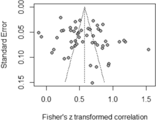
In this paper, we present first ever meta-analysis of impacts of weather on the death and incidence on the COVID-19. Initially, we selected vital articles from digital repositories to find resourceful information. Thus, we performed a systematic review upon proper inclusion and exclusion criteria. Secondly, we used risk assessment of the included articles in this study. Thirdly, we performed evidence certainty tests of such articles to find suitability over the significant impact analysis of weather over COVID-19. We selected five weather parameter such as, temperature, humidity, rainfall, ultra violet and wind speed to find correlation with the death rate and incidence of the COVID-19. Fourthly, we performed forest and funnel plots to investigate the heterogeneity and publication bias, respectively.

Search strategy

A comprehensive literature survey was conducted while considering articles from the following digital databases such as, PubMed, Sciencedirect, IEEE Xplore, Google Scholar, and Cochrane. We used a set of combination of key words to search the articles as shown in Table 1 . One independent author (PPR) performed screening of abstract and titles of the literature against the aforementioned keyword and scope of the study. Other author (PM) did the review of final selection of the articles. Evaluation of full-texts were conducted against the inclusion and exclusion criteria.

Study selection

The work was done as per the Preferred Reporting Items for Systematic Reviews and Meta-Analyses (PRISMA) guidelines 28 . We conducted a qualitative analysis of the 11 included articles in this study based on publication year, zone or country of work, various variables used, key techniques used and remarks on the observations. Figure 1 presents the PRISMA of the meta-analysis. Inclusion of articles depends on the availability of correlation factors in the surveyed articles. We have included those studies that only discusses about the correlation between weather parameters to COVID-19. We also, seek for the relevance of performed studies in the article to prescribe some key suggestions. Further, we include those articles that are full-text published but not from the medRxiv repository for meta-analysis. We focused on the quantitative synthesis of statistical approaches used in the articles. We excluded all the articles which are published in non-indexed journals and don’t conform to the direct correlation perspective of COVID-19 with weather factors. Due to lack of minimal availability, we exclude the correlating parameters related to the pollution, air quality index (AQI), pollination, and sun light intensity as the weather parameters in this meta-analysis.

PRISMA flowchart for the study.

Forest plot of COVID-19 death rate with temperature.

Assessment of risk of bias

We assessed the quality of the articles selected in this study by using the Joanna Briggs Institute (JBI) tool 29 . The checklist contained eight questions such as (a) were the criteria for inclusion in the sample clearly defined, (b) were the study subjects and the setting described in detail, (c) was the exposure measured in a valid and reliable way, were objective, (d) standard criteria used for measurement of the condition, (e) were confounding factors identified, (f) were strategies to deal with confounding factors stated, (g) were the outcomes measured in a valid and reliable way and (h) was appropriate statistical analysis used. Each of the question was examined against each of the 11 articles and answer was given in ‘Yes’ and ‘No’. Overall risk was finally specified at the bottom of Table 2 with two main answers such as, ‘Low’ and ‘Moderate’. Both the authors (PPR and PM) independently evaluated risk and quality of each study and confusion was mitigated by a consensus team meeting.

Data extraction and outcome measure

Data was extracted for following variables such as, (a) temperature, (b) humidity, (c) rainfall, (d) ultra violet (UV) radiation and (e) wind speed. We considered two key COVID-19 parameters such as, (a) death rate and (b) incidence. Thus, five key weather elements were used to find association with two COVID-19 parameters for performing meta-analysis on possible weather impact on COVID-19. Solar radiation and UV radiation were assumed to be same by considering SI unit i.e. W-m -2 . We considered relative humidity out of absolute and relative humidity while performing this meta-analysis. Major characteristics of the included studies rely in the recently performed correlation assessment between the weather parameters with the incidence or death rate of COVID-19. Further, we considered the evaluation criteria as mentioned in the articles to provide the meta-analysis.

Certainty measure

The GRADE (Grading of Recommendations Assessment, Development, and Evaluation) 30 approach was used to evaluate the quality of evidence for each outcome as shown in Table 3 . We tested 7 outcomes on the correlations between (a) temperature and COVID-19 death rate, (b) humidity with COVID-19 death rate, (c) temperature with COVID-19 incidence, (d) humidity with COVID-19 incidence, (e) rainfall with COVID-19 incidence, (f) UV with COVID-19 incidence, and (g) wind speed with COVID-19 incidence. We found the impact of each of the outcomes. We also measured the evidence of certainty using  ⊕  AND/OR ◯ combination of four symbols in terms of ‘Moderate’, ‘High’, and ‘Very High’. The points in the GRADE analysis are considered as follows. Very High point is given to the correlation factor that shows the highest order significance among all the included works. Similarly, High point is given to those parametrization aspects where we notice strong evidence of measure. We give Moderate as the lowest measure to the correlating perspective having lowest of significance.

Statistical analysis

Accessed data from 11 articles were initially recorded into the excel datasheet which was later segregated into 7 different comma separated value CSV) files for feeding into the RStudio version 3.4.3 with package meta. We used metacor(cor = r, n = N, data = d, studlab = Author, sm = "ZCOR") method call to perform the fixed-effect and random effect model study. We used Fisher’s z transformed correlations to find meta-analysis. Here, r, N and d represent the CSV columns named as r, N and the CSV itself, respectively. Where, r and N (sample size) of the specific CSV stored the correlation values in ( +) and/or (-) terms and days of experiment by individual article, respectively. 95% confidence interval (CI) was measured for each of the articles. Wang et al. (2020a), Wang et al. (2020b), Meo et al. (2020a), and Meo et al. (2020b) were sub-set wise used of the Wang et al. (2020) and Meo et al. (2020) articles, respectively. Fixed and random weight of each of the article was computed. We found heterogeneity (I 2 ) and τ 2 as the level of heterogeneity and measure of dispersion of true effect sizes under the given assumptions that the true effect sizes were bell-shaped and normally distributed, respectively. We used the forest() method to derive the forest plots for seven different scenarios of correlation meta-analysis with help of the Fisher's z transformed correlations.

Study selection and characteristics

The article reporting and record keeping task was finalized on August 6, 2020. All the included papers belong to the initial to recent COVID-19 impacts i.e. December 1, 2019–June 5, 2020. Based on initial record screening, we found 453 articles. We remove 381 irrelevant articles and later moved with 72 records. Due to irrelevance to weather parametric data selection, measurement and study approaches, we excluded 27 articles. Out of 45 articles, upon full-text screening we found improper statistical data and insignificant association between weather and COVID-19, we rejected 14 articles. Rest of the 37 articles were focused on wither parametric or description statistical association study between the weather and COVID-19. However, 23 were found to be nonconclusive toward correlation between weather and COVID-19 which were later on rejected. Out of 14 articles, only 11 were finally included in this meta-analysis. All the studies discussed about some sort of correlation factor with one or more weather parameters comprising of temperature, humidity, rainfall, UV and wind speed with the COVID-19 death rate or incidence level in various parts of globe. The articles conducted studies in different zones of countries belonging to Wuhan, China, mainland China, India, USA, Japan, Jakarta, Indonesia, Australia, Canada, Iran and more than 110 countries. The article mainly used the Pearson’s correlation coefficient, cohort study, Spearman’s rank correlation logarithmic estimation, generalized additive model (GAM) and Fama–Macbeth regression statistical techniques. Out of 11 only 1 article remarked about the basic reproduction number i.e. R 0 in conjunction to the weather parameters for possible impact on the COVID-19 incidence.

Survey of articles

Table 4 presents the comparison between the articles included in this study. Wang et al. (2020a) and Wang et al. (2020b) represent a single article but two different works related to China and USA. Similarly, Meo et al. (2020) performed studies on 10 hottest and 10 coolest countries, thus two versions of citations were used into the further works such as Meo et al. (2020a) and Meo et al. (2020b) representing hot and cool countries, respectively.

Overall outcomes

Table 5 presents overall outcome from this study. Correlation between the temperature and COVID-19 death rate was measured as (a) fixed effect model: 0.11 (95% CI, 0.01–0.22) and (b) random effect model: 0.21 (95% CI − 0.14–0.52) with p  < 0.01. Similarly, humidity and COVID-19 correlation were measured as − 0.13 (95% CI, − 0.23- 0.03) and − 0.13 (95% CI, − 0.23–0.03) for fixed and random effect model, respectively against p-value at 0.53.

In case of weather and COVID-19 incidence correlation aspect, we found that temperature had 0.22 (95% CI, 0.16–0.28) and 0.23 (95% CI, 0.01–0.42) for fixed and random study, respectively. We found that humidity had positive correlation with the COVID-19 incidence at p  < 0.01. Rainfall had minimal positive correlation with COVID-19 incidence having 0.04 (95% CI, − 0.09–0.16)0.03 (95% CI, − 0.10–0.17) for fixed and random, respectively. Correlation between UV and COVID-19 incidence was measured as − 0.09 (95% CI, − 0.23–0.06) for fixed and − 0.14 (95% CI, − 0.43–0.18) for random model. Wind speed was found to have positive correlation with the incidence of COVID-19 such as, 0.58 (95% CI, 0.49–0.66) and 0.62 (95% CI, − 0.17–0.92).

Heterogeneity (I 2 ) was mostly observed with the temperature, humidity (COVID-19 incidence) and wind speed variables i.e. 90%, 96% and 98%, respectively. Complete homogeneity i.e. (I 2  = 0) was found in the humidity with the death rate of COVID-19 with zero τ 2 . I 2 of rainfall was found as 16% against the COVID-19 incidence.

Figures 2 , 3 , 4 , 5 , 6 , 7 , and 8 present the forest plots of seven different correlation aspects of weather parameters with COVID-19 death rate and incidence.

Forest plot of COVID-19 death rate with humidity.

Forest plot of COVID-19 incidence with temperature.

Forest plot of COVID-19 incidence with humidity.

Forest plot of COVID-19 incidence with rainfall.

Forest plot of COVID-19 incidence with UV.

Forest plot of COVID-19 incidence with wind speed.

To best of our knowledge, herein presented systematic review and meta-analysis is the first ever work to find answer of correlation between weather on COVID-19. Our meta-analysis is the first to analyse the effect of weather on the death rate and incidence of COVID-19. Based on our meta-analysis we found correlation between weather on the COVID-19. Temperature and humidity are most crucial weather factors that are string enough to impact over the death rate and incidence of COVID-19 42 , 43 . All the articles included into this study adhere to the weather centric approaches to the COVID-19. All the articles performed their research during December, 2019 to June, 2020. Thus, a long-time duration was covered in our meta-analysis to come at genuine and effective conclusion about possibility of weather impact on COVID-19. Correlation parameters were used in this study to disseminate direct relationship between the weather and COVID-19.

Our meta-analysis included more than 110 country data regarding weather impact on the coronavirus spread and deaths. As the articles carries extensive research during initial phase and mid phase of COVID-19 in most of the countries, this meta-analysis is far more effective to provide more specific answer to correlation-related questions which were frequently asked in near past. With involvement of the JBI tools and GRADE evidence profile, presented meta-analysis serves as an indispensable literature in the current context of COVID-19 incidence.

In this meta-analysis, we assumed the correlation values to be most effective than other alternatives due to its straight forward nature of relationship measurement approach. We depended our study over the fixed and random effect models asides the heterogeneity and dispersion of true size effects. Significant forest plots were obtained for the (a) temperature versus death rate, (b) temperature versus incidence, (c) humidity versus incidence, and (d) wind speed versus incidence of COVID-19 i.e. air borne. Though, impact of UV radiation over the incidence of COVID-19 was computed but negative correlation was observed. It means that with more UV radiation lesser incidence of COVID-19 can be found. Similarly, rainfall has a positive correlation with COVID-19 incidence.

We didn’t know the exact reason why such behaviour i.e. non-significance was observed. We can hypothesize that higher rainfall increases relative humidity in air thus a greater number of cases can be seen due to COVID-19. One surprising result was found in our meta-analysis i.e. negative correlation between humidity with death rate, though its relationship to the incidence was earlier discussed to be positively correlated. We not clear about the reason behind such nature of humidity.

Our work has some limitations including availability of plentiful research on weather correlation with COVID-19. This study restricted us to conduct meta-analysis on available articles where some of them were taken from various preprint servers. Thus, risk of rejection of those articles were not accurately considered, even though we used JBI and GRADE methods. We can also say that hot countries with high average temperature and relative humidity are more prone get affected by new incidences of COVID-19 in coming days. It can be estimated that during coming winter may provide some relief to the people of world. However, more research should be conducted to better support our meta-analysis conclusions.

We found some strong correlations between weather over the incidence of COVID-19. The met-a analysis can be useful for the policy makers of the government and health incorporations to take prior decisions before the possible surge of COVID-19 cases depending on the weather forecasting mechanism. We urge the medical professionals and weather analysts to further investigate the findings of this article as the a-priori information to mitigate the COVID-19 pandemic.

COVID, T.C. and Team, R. Severe outcomes among patients with coronavirus disease 2019 (COVID-19)-United States, February 12-March 16, 2020. MMWR Morb Mortal Wkly Rep 69 (12), 343–346 (2020).

Article   Google Scholar  

Mehta, P. et al. COVID-19: consider cytokine storm syndromes and immunosuppression. Lancet (London, England) 395 (10229), 1033 (2020).

Article   CAS   Google Scholar  

Velavan, T. P. & Meyer, C. G. The COVID-19 epidemic. Tropical Med. Int. Health 25 (3), 278 (2020).

Kannan, S., Ali, P. S. S., Sheeza, A. & Hemalatha, K. COVID-19 (Novel Coronavirus 2019)-recent trends. Eur. Rev. Med. Pharmacol. Sci 24 (4), 2006–2011 (2020).

CAS   PubMed   Google Scholar  

Worldometer covid-19, Available online https://www.worldometers.info/coronavirus/ , Accessed on September 1, 2020.

Le, T. T. et al. The COVID-19 vaccine development landscape. Nat. Rev. Drug Discov. 19 (5), 305–306 (2020).

Hotez, P. J., Corry, D. B. & Bottazzi, M. E. COVID-19 vaccine design: the Janus face of immune enhancement. Nat. Rev. Immunol. 20 (6), 347–348 (2020).

Graham, B. S. Rapid COVID-19 vaccine development. Science 368 (6494), 945–946 (2020).

Corey, L., Mascola, J. R., Fauci, A. S. & Collins, F. S. A strategic approach to COVID-19 vaccine R&D. Science 368 (6494), 948–950 (2020).

Wu, S.C., 2020. Progress and Concept for COVID‐19 Vaccine Development. Biotechnology Journal.

Yamey, G. et al. Ensuring global access to COVID-19 vaccines. The Lancet 395 (10234), 1405–1406 (2020).

Lv, H., Wu, N.C. and Mok, C.K., 2020. COVID‐19 vaccines: knowing the unknown. European J. Immunol .

Koirala, A., Joo, Y.J., Khatami, A., Chiu, C. and Britton, P.N., 2020. Vaccines for COVID-19: the current state of play. Paediatric Respirat. Rev .

DeRoo, S.S., Pudalov, N.J. and Fu, L.Y., 2020. Planning for a COVID-19 Vaccination Program. JAMA .

Thunstrom, L., Ashworth, M., Finnoff, D. and Newbold, S., 2020. Hesitancy Towards a COVID-19 Vaccine and Prospects for Herd Immunity. Available at SSRN 3593098.

Kyle, C. H., Liu, J., Gallagher, M. E., Dukic, V. & Dwyer, G. Stochasticity and infectious disease dynamics: density and weather effects on a fungal insect pathogen. Am. Nat. 195 (3), 504–523 (2020).

Fujii, F., Egami, N., Inoue, M. and Koga, H., 2020. Weather condition, air pollutants, and epidemics as factors that potentially influence the development of Kawasaki disease. Sci. Total Environ , 741, p.140469.

Wang, Z.B., Ren, L., Lu, Q.B., Zhang, X.A., Miao, D., Hu, Y.Y., Dai, K., Li, H., Luo, Z.X., Fang, L.Q. and Liu, E.M., 2020. The impact of weather and air pollution on viral infection and disease outcome among pediatric pneumonia patients in Chongqing, China from 2009 to 2018: a prospective observational study. Clinical Infectious Diseases.

Passer, J.K., Danila, R.N., Laine, E.S., Como-Sabetti, K.J., Tang, W. and Searle, K.M., 2020. The association between sporadic Legionnaires' disease and weather and environmental factors, Minnesota, 2011–2018. Epidemiology & Infection, 148.

Tobías, A. & Molina, T. Is temperature reducing the transmission of COVID-19?. Environ. Res. 186 , 109553 (2020).

Yuan, S., Jiang, S. & Li, Z. L. Do humidity and temperature impact the spread of the novel coronavirus?. Front. Public Health 8 , 240 (2020).

Anis, A., 2020. The Effect of Temperature Upon Transmission of COVID-19: Australia And Egypt Case Study. Available at SSRN 3567639.

Mecenas, P., Bastos, R., Vallinoto, A. and Normando, D., 2020. Effects of temperature and humidity on the spread of COVID-19: a systematic review. medRxiv.

Harmooshi, N.N., Shirbandi, K. and Rahim, F., 2020. Environmental concern regarding the effect of humidity and temperature on 2019-nCoV survival: fact or fiction. Environmental Science and Pollution Research, pp.1–10.

Gupta, S., Raghuwanshi, G.S. and Chanda, A., 2020. Effect of weather on COVID-19 spread in the US: a prediction model for India in 2020. Science of The Total Environment, p.138860.

Şahin, M., 2020. Impact of weather on COVID-19 pandemic in Turkey. Science of The Total Environment, p.138810.

Rosario, D.K., Mutz, Y.S., Bernardes, P.C. and Conte-Junior, C.A., 2020. Relationship between COVID-19 and weather: Case study ain a tropical country. Int. J. Hyg. Environ. Health, 229, p.113587.

Chen, H. et al. Compound Kushen injection combined with platinum-based chemotherapy for stage III/IV non-small cell lung cancer: a meta-analysis of 37 RCTs following the PRISMA guidelines. J. Cancer 11 (7), 1883 (2020).

Lockwood, C., Stannard, D., Jordan, Z. and Porritt, K., 2020. The Joanna Briggs Institute clinical fellowship program: a gateway opportunity for evidence-based quality improvement and organizational culture change.

Piggott, T., Morgan, R.L., Cuello-Garcia, C.A., Santesso, N., Mustafa, R.A., Meerpohl, J.J., Schünemann, H.J. and GRADE Working Group. Grading of Recommendations Assessment, Development, and Evaluations (GRADE) notes: extremely serious, GRADE’s terminology for rating down by three levels. J. Clin. Epidemiol. 120 , 116–120 (2020).

Ma, Y., Zhao, Y., Liu, J., He, X., Wang, B., Fu, S., Yan, J., Niu, J., Zhou, J. and Luo, B., 2020. Effects of temperature variation and humidity on the death of COVID-19 in Wuhan, China. Science of The Total Environment, p.138226.

Wang, J., Tang, K., Feng, K. and Lv, W., 2020. High temperature and high humidity reduce the transmission of COVID-19. Available at SSRN 3551767.

Nazrul, I., Sharmin, S. and Mesut, E.A., 2020. Temperature, humidity, and wind speed are associated with lower Covid-19 incidence. https://www.medrxiv.org/content/medrxiv/early/2020/03/31/2020.03.27.20045658.full.pdf .

Qi, H., Xiao, S., Shi, R., Ward, M.P., Chen, Y., Tu, W., Su, Q., Wang, W., Wang, X. and Zhang, Z., 2020. COVID-19 transmission in Mainland China is associated with temperature and humidity: a time-series analysis. Science of the Total Environment, p.138778.

Meo, S. A. et al. Climate and COVID-19 pandemic: effect of heat and humidity on the incidence and mortality in world’s top ten hottest and top ten coldest countries. Eur. Rev. Med. Pharmacol. Sci. 24 (15), 8232–8238 (2020).

Rashed, E. A., Kodera, S., Gomez-Tames, J. & Hirata, A. Influence of absolute humidity, temperature and population density on COVID-19 spread and decay durations: multi-prefecture study in Japan. Int. J. Environ. Res. Public Health 17 (15), 5354 (2020).

Tosepu, R., Gunawan, J., Effendy, D.S., Lestari, H., Bahar, H. and Asfian, P., 2020. Correlation between weather and Covid-19 pandemic in Jakarta, Indonesia. Sci. Total Environ , p.138436.

Bashir, M. F. et al. Correlation between climate indicators and COVID-19 pandemic in New York 138835 (Science of The Total Environment, 2020).

Google Scholar  

Vinoj, V., Gopinath, N., Landu, K., Behera, B. and Mishra, B., 2020. The COVID-19 Spread in India and its dependence on temperature and relative humidity.

Sajadi, M.M., Habibzadeh, P., Vintzileos, A., Shokouhi, S., Miralles-Wilhelm, F. and Amoroso, A., 2020. Temperature and latitude analysis to predict potential spread and seasonality for COVID-19. Available at SSRN 3550308.

Xu, R., Rahmandad, H., Gupta, M., DiGennaro, C., Ghaffarzadegan, N., Amini, H. and Jalali, M.S., 2020. The modest impact of weather and air pollution on COVID-19 transmission. medRxiv.

Hariyanto, T. I., Kristine, E., Jillian Hardi, C. & Kurniawan, A. Efficacy of lopinavir/ritonavir compared with standard care for treatment of coronavirus disease 2019 (COVID-19): a systematic review. Infect. Disord. Drug Targets. https://doi.org/10.2174/1871526520666201029125725 (2020).

Article   PubMed   Google Scholar  

Hariyanto, T. I., Hardyson, W. & Kurniawan, A. Efficacy and safety of tocilizumab for coronavirus disease 2019 (Covid-19) patients: a systematic review and meta-analysis. Drug Res. (Stuttg). https://doi.org/10.1055/a-1336-2371 (2021).

Download references

Author information

Authors and affiliations.

Department of Biotechnology, Maulana Abul Kalam Azad University of Technology, Kolkata, India

Poulami Majumder

Department of Computer Applications, Sikkim University, Gangtok, India

Partha Pratim Ray

You can also search for this author in PubMed   Google Scholar

Contributions

P.M. gathered data and designed the experiments. P.P.R. wrote the paper and performed the analysis. All authors reviewed the manuscript.

Corresponding author

Correspondence to Partha Pratim Ray .

Ethics declarations

Competing interests.

The authors declare no competing interests.

Additional information

Publisher's note.

Springer Nature remains neutral with regard to jurisdictional claims in published maps and institutional affiliations.

Rights and permissions

Open Access This article is licensed under a Creative Commons Attribution 4.0 International License, which permits use, sharing, adaptation, distribution and reproduction in any medium or format, as long as you give appropriate credit to the original author(s) and the source, provide a link to the Creative Commons licence, and indicate if changes were made. The images or other third party material in this article are included in the article's Creative Commons licence, unless indicated otherwise in a credit line to the material. If material is not included in the article's Creative Commons licence and your intended use is not permitted by statutory regulation or exceeds the permitted use, you will need to obtain permission directly from the copyright holder. To view a copy of this licence, visit http://creativecommons.org/licenses/by/4.0/ .

Reprints and permissions

About this article

Cite this article.

Majumder, P., Ray, P.P. A systematic review and meta-analysis on correlation of weather with COVID-19. Sci Rep 11 , 10746 (2021). https://doi.org/10.1038/s41598-021-90300-9

Download citation

Received : 17 December 2020

Accepted : 10 May 2021

Published : 24 May 2021

DOI : https://doi.org/10.1038/s41598-021-90300-9

Share this article

Anyone you share the following link with will be able to read this content:

Sorry, a shareable link is not currently available for this article.

Provided by the Springer Nature SharedIt content-sharing initiative

This article is cited by

Association of air pollution and weather conditions during infection course with covid-19 case fatality rate in the united kingdom.

• M. Pear Hossain
• Hsiang-Yu Yuan

Scientific Reports (2024)

Bell correlations outside physics

• E. M. Pothos
• B. W. Wojciechowski

Scientific Reports (2023)

Human exposure risk assessment for infectious diseases due to temperature and air pollution: an overview of reviews

• Xuping Song

Environmental Science and Pollution Research (2023)

Scientific Reports (2022)

By submitting a comment you agree to abide by our Terms and Community Guidelines . If you find something abusive or that does not comply with our terms or guidelines please flag it as inappropriate.

Quick links

• Explore articles by subject
• Guide to authors
• Editorial policies

Sign up for the Nature Briefing: Anthropocene newsletter — what matters in anthropocene research, free to your inbox weekly.

• SUGGESTED TOPICS
• The Magazine
• Newsletters
• Managing Yourself
• Managing Teams
• Work-life Balance
• The Big Idea
• Data & Visuals
• Reading Lists
• Case Selections
• HBR Learning
• Topic Feeds
• Account Settings
• Email Preferences

How to Use Correlation to Make Predictions

• Dean Karlan
• Michael Luca

Don’t overlook a useful pattern just because it isn’t driven by a causal relationship.

Leaders too often misinterpret empirical patterns and miss opportunities to engage in data-driven thinking. To better leverage data, leaders need to understand the types of problems data can help solve as well as the difference between those problems that can be solved with improved prediction and those that can be solved with a better understanding of causation.

Too many leaders take an incomplete approach to understanding empirical patterns, leading to costly mistakes and misinterpretations. As we have discussed before , one extremely common mistake is interpreting a misleading correlation as causal. We’ve advised countless organizations on the topic. We’ve written research papers, managerial articles, and even a book dedicated to the power of experiments and causal inference tools — a toolkit that economists have adopted and adapted over the past few decades. Yet, while we are deep believers in the causal inference toolkit, we’ve also seen the reverse problem — leaders who overlook useful patterns because they are not causal. The truth is, there are also times when a correlation is not only sufficient, but is exactly what is needed. The mistake leaders make here is failing to understand the distinction between prediction and causation. Or, more specifically, the distinction between predicting an outcome and predicting how a decision will affect an outcome.

• DK Dean Karlan is a professor at Northwestern’s Kellogg School of Management and founder of Innovations for Poverty Action.
• Michael Luca is the Lee J. Styslinger III Associate Professor of Business Administration at Harvard Business School and a coauthor (with Max H. Bazerman) of The Power of Experiments: Decision Making in a Data-Driven World (forthcoming from MIT Press).

Partner Center

Have a language expert improve your writing

Run a free plagiarism check in 10 minutes, generate accurate citations for free.

• Knowledge Base
• Pearson Correlation Coefficient (r) | Guide & Examples

Pearson Correlation Coefficient (r) | Guide & Examples

Published on May 13, 2022 by Shaun Turney . Revised on February 10, 2024.

The Pearson correlation coefficient ( r ) is the most common way of measuring a linear correlation. It is a number between –1 and 1 that measures the strength and direction of the relationship between two variables.

Table of contents

What is the pearson correlation coefficient, visualizing the pearson correlation coefficient, when to use the pearson correlation coefficient, calculating the pearson correlation coefficient, testing for the significance of the pearson correlation coefficient, reporting the pearson correlation coefficient, other interesting articles, frequently asked questions about the pearson correlation coefficient.

The Pearson correlation coefficient ( r ) is the most widely used correlation coefficient and is known by many names:

• Pearson’s r
• Bivariate correlation
• Pearson product-moment correlation coefficient (PPMCC)
• The correlation coefficient

The Pearson correlation coefficient is a descriptive statistic , meaning that it summarizes the characteristics of a dataset. Specifically, it describes the strength and direction of the linear relationship between two quantitative variables.

Although interpretations of the relationship strength (also known as effect size ) vary between disciplines, the table below gives general rules of thumb:

The Pearson correlation coefficient is also an inferential statistic , meaning that it can be used to test statistical hypotheses . Specifically, we can test whether there is a significant relationship between two variables.

Prevent plagiarism. Run a free check.

Another way to think of the Pearson correlation coefficient ( r ) is as a measure of how close the observations are to a line of best fit .

The Pearson correlation coefficient also tells you whether the slope of the line of best fit is negative or positive. When the slope is negative, r is negative. When the slope is positive, r is positive.

When r is 1 or –1, all the points fall exactly on the line of best fit:

When r is greater than .5 or less than –.5, the points are close to the line of best fit:

When r is between 0 and .3 or between 0 and –.3, the points are far from the line of best fit:

When r is 0, a line of best fit is not helpful in describing the relationship between the variables:

The Pearson correlation coefficient ( r ) is one of several correlation coefficients that you need to choose between when you want to measure a correlation. The Pearson correlation coefficient is a good choice when all of the following are true:

• Both variables are quantitative : You will need to use a different method if either of the variables is qualitative .
• The variables are normally distributed : You can create a histogram of each variable to verify whether the distributions are approximately normal. It’s not a problem if the variables are a little non-normal.
• The data have no outliers : Outliers are observations that don’t follow the same patterns as the rest of the data. A scatterplot is one way to check for outliers—look for points that are far away from the others.
• The relationship is linear: “Linear” means that the relationship between the two variables can be described reasonably well by a straight line. You can use a scatterplot to check whether the relationship between two variables is linear.

Pearson vs. Spearman’s rank correlation coefficients

Spearman’s rank correlation coefficient is another widely used correlation coefficient. It’s a better choice than the Pearson correlation coefficient when one or more of the following is true:

• The variables are ordinal .
• The variables aren’t normally distributed .
• The data includes outliers.
• The relationship between the variables is non-linear and monotonic.

Below is a formula for calculating the Pearson correlation coefficient ( r ):

The formula is easy to use when you follow the step-by-step guide below. You can also use software such as R or Excel to calculate the Pearson correlation coefficient for you.

Step 1: Calculate the sums of x and y

Start by renaming the variables to “ x ” and “ y .” It doesn’t matter which variable is called x and which is called y —the formula will give the same answer either way.

Next, add up the values of x and y . (In the formula, this step is indicated by the Σ symbol, which means “take the sum of”.)

Σ x = 3.63 + 3.02 + 3.82 + 3.42 + 3.59 + 2.87 + 3.03 + 3.46 + 3.36 + 3.30

Σ y = 53.1 + 49.7 + 48.4 + 54.2 + 54.9 + 43.7 + 47.2 + 45.2 + 54.4 + 50.4

Step 2: Calculate x 2 and y 2 and their sums

Create two new columns that contain the squares of x and y . Take the sums of the new columns.

Σ x 2  = 13.18 + 9.12 + 14.59 + 11.70 + 12.89 +  8.24 +  9.18 + 11.97 + 11.29 + 10.89

Σ x 2  = 113.05

Σ y 2  = 2 819.6 + 2 470.1 + 2 342.6 + 2 937.6 + 3 014.0 + 1 909.7 + 2 227.8 + 2 043.0 + 2 959.4 + 2 540.2

Step 3: Calculate the cross product and its sum

In a final column, multiply together x and y (this is called the cross product). Take the sum of the new column.

Σ xy = 192.8 + 150.1 + 184.9 + 185.4 + 197.1 + 125.4 + 143.0 + 156.4 + 182.8 + 166.3

Step 4: Calculate r

Use the formula and the numbers you calculated in the previous steps to find r .

Here's why students love Scribbr's proofreading services

Discover proofreading & editing

The Pearson correlation coefficient can also be used to test whether the relationship between two variables is significant .

The Pearson correlation of the sample is r . It is an estimate of rho ( ρ ), the Pearson correlation of the population . Knowing r and n (the sample size), we can infer whether ρ is significantly different from 0.

• Null hypothesis ( H 0 ): ρ = 0
• Alternative hypothesis ( H a ): ρ ≠ 0

To test the hypotheses , you can either use software like R or Stata or you can follow the three steps below.

Step 1: Calculate the t value

Calculate the t value (a test statistic ) using this formula:

Step 2: Find the critical value of t

You can find the critical value of t ( t* ) in a t table. To use the table, you need to know three things:

• The degrees of freedom ( df ): For Pearson correlation tests, the formula is df = n – 2.
• Significance level (α): By convention, the significance level is usually .05.
• One-tailed or two-tailed: Most often, two-tailed is an appropriate choice for correlations.

Step 3: Compare the t value to the critical value

Determine if the absolute t value is greater than the critical value of t . “Absolute” means that if the t value is negative you should ignore the minus sign.

Step 4: Decide whether to reject the null hypothesis

• If the t value is greater than the critical value, then the relationship is statistically significant ( p <  α ). The data allows you to reject the null hypothesis and provides support for the alternative hypothesis.
• If the t value is less than the critical value, then the relationship is not statistically significant ( p >  α ). The data doesn’t allow you to reject the null hypothesis and doesn’t provide support for the alternative hypothesis.

If you decide to include a Pearson correlation ( r ) in your paper or thesis, you should report it in your results section . You can follow these rules if you want to report statistics in APA Style :

• You don’t need to provide a reference or formula since the Pearson correlation coefficient is a commonly used statistic.
• You should italicize r when reporting its value.
• You shouldn’t include a leading zero (a zero before the decimal point) since the Pearson correlation coefficient can’t be greater than one or less than negative one.
• You should provide two significant digits after the decimal point.

When Pearson’s correlation coefficient is used as an inferential statistic (to test whether the relationship is significant), r is reported alongside its degrees of freedom and p value. The degrees of freedom are reported in parentheses beside r .

If you want to know more about statistics , methodology , or research bias , make sure to check out some of our other articles with explanations and examples.

• Chi square test of independence
• Statistical power
• Descriptive statistics
• Degrees of freedom
• Null hypothesis

Methodology

• Double-blind study
• Case-control study
• Research ethics
• Data collection
• Hypothesis testing
• Structured interviews

Research bias

• Hawthorne effect
• Unconscious bias
• Recall bias
• Halo effect
• Self-serving bias
• Information bias

You should use the Pearson correlation coefficient when (1) the relationship is linear and (2) both variables are quantitative and (3) normally distributed and (4) have no outliers.

You can use the cor() function to calculate the Pearson correlation coefficient in R. To test the significance of the correlation, you can use the cor.test() function.

You can use the PEARSON() function to calculate the Pearson correlation coefficient in Excel. If your variables are in columns A and B, then click any blank cell and type “PEARSON(A:A,B:B)”.

There is no function to directly test the significance of the correlation.

Cite this Scribbr article

If you want to cite this source, you can copy and paste the citation or click the “Cite this Scribbr article” button to automatically add the citation to our free Citation Generator.

Turney, S. (2024, February 10). Pearson Correlation Coefficient (r) | Guide & Examples. Scribbr. Retrieved April 15, 2024, from https://www.scribbr.com/statistics/pearson-correlation-coefficient/

Is this article helpful?

Shaun Turney

Other students also liked, simple linear regression | an easy introduction & examples, coefficient of determination (r²) | calculation & interpretation, hypothesis testing | a step-by-step guide with easy examples, what is your plagiarism score.

• Privacy Policy

Buy Me a Coffee

Home » Correlation Analysis – Types, Methods and Examples

Correlation Analysis – Types, Methods and Examples

Table of Contents

Correlation Analysis

Correlation analysis is a statistical method used to evaluate the strength and direction of the relationship between two or more variables . The correlation coefficient ranges from -1 to 1.

• A correlation coefficient of 1 indicates a perfect positive correlation. This means that as one variable increases, the other variable also increases.
• A correlation coefficient of -1 indicates a perfect negative correlation. This means that as one variable increases, the other variable decreases.
• A correlation coefficient of 0 means that there’s no linear relationship between the two variables.

Correlation Analysis Methodology

Conducting a correlation analysis involves a series of steps, as described below:

• Define the Problem : Identify the variables that you think might be related. The variables must be measurable on an interval or ratio scale. For example, if you’re interested in studying the relationship between the amount of time spent studying and exam scores, these would be your two variables.
• Data Collection : Collect data on the variables of interest. The data could be collected through various means such as surveys , observations , or experiments. It’s crucial to ensure that the data collected is accurate and reliable.
• Data Inspection : Check the data for any errors or anomalies such as outliers or missing values. Outliers can greatly affect the correlation coefficient, so it’s crucial to handle them appropriately.
• Choose the Appropriate Correlation Method : Select the correlation method that’s most appropriate for your data. If your data meets the assumptions for Pearson’s correlation (interval or ratio level, linear relationship, variables are normally distributed), use that. If your data is ordinal or doesn’t meet the assumptions for Pearson’s correlation, consider using Spearman’s rank correlation or Kendall’s Tau.
• Compute the Correlation Coefficient : Once you’ve selected the appropriate method, compute the correlation coefficient. This can be done using statistical software such as R, Python, or SPSS, or manually using the formulas.
• Interpret the Results : Interpret the correlation coefficient you obtained. If the correlation is close to 1 or -1, the variables are strongly correlated. If the correlation is close to 0, the variables have little to no linear relationship. Also consider the sign of the correlation coefficient: a positive sign indicates a positive relationship (as one variable increases, so does the other), while a negative sign indicates a negative relationship (as one variable increases, the other decreases).
• Check the Significance : It’s also important to test the statistical significance of the correlation. This typically involves performing a t-test. A small p-value (commonly less than 0.05) suggests that the observed correlation is statistically significant and not due to random chance.
• Report the Results : The final step is to report your findings. This should include the correlation coefficient, the significance level, and a discussion of what these findings mean in the context of your research question.

Types of Correlation Analysis

Types of Correlation Analysis are as follows:

Pearson Correlation

This is the most common type of correlation analysis. Pearson correlation measures the linear relationship between two continuous variables. It assumes that the variables are normally distributed and have equal variances. The correlation coefficient (r) ranges from -1 to +1, with -1 indicating a perfect negative linear relationship, +1 indicating a perfect positive linear relationship, and 0 indicating no linear relationship.

Spearman Rank Correlation

Spearman’s rank correlation is a non-parametric measure that assesses how well the relationship between two variables can be described using a monotonic function. In other words, it evaluates the degree to which, as one variable increases, the other variable tends to increase, without requiring that increase to be consistent.

Kendall’s Tau

Kendall’s Tau is another non-parametric correlation measure used to detect the strength of dependence between two variables. Kendall’s Tau is often used for variables measured on an ordinal scale (i.e., where values can be ranked).

Point-Biserial Correlation

This is used when you have one dichotomous and one continuous variable, and you want to test for correlations. It’s a special case of the Pearson correlation.

Phi Coefficient

This is used when both variables are dichotomous or binary (having two categories). It’s a measure of association for two binary variables.

Canonical Correlation

This measures the correlation between two multi-dimensional variables. Each variable is a combination of data sets, and the method finds the linear combination that maximizes the correlation between them.

Partial and Semi-Partial (Part) Correlations

These are used when the researcher wants to understand the relationship between two variables while controlling for the effect of one or more additional variables.

Cross-Correlation

Used mostly in time series data to measure the similarity of two series as a function of the displacement of one relative to the other.

Autocorrelation

This is the correlation of a signal with a delayed copy of itself as a function of delay. This is often used in time series analysis to help understand the trend in the data over time.

Correlation Analysis Formulas

There are several formulas for correlation analysis, each corresponding to a different type of correlation. Here are some of the most commonly used ones:

Pearson’s Correlation Coefficient (r)

Pearson’s correlation coefficient measures the linear relationship between two variables. The formula is:

   r = Σ[(xi – Xmean)(yi – Ymean)] / sqrt[(Σ(xi – Xmean)²)(Σ(yi – Ymean)²)]

• xi and yi are the values of X and Y variables.
• Xmean and Ymean are the mean values of X and Y.
• Σ denotes the sum of the values.

Spearman’s Rank Correlation Coefficient (rs)

Spearman’s correlation coefficient measures the monotonic relationship between two variables. The formula is:

   rs = 1 – (6Σd² / n(n² – 1))

• d is the difference between the ranks of corresponding variables.
• n is the number of observations.

Kendall’s Tau (τ)

Kendall’s Tau is a measure of rank correlation. The formula is:

   τ = (nc – nd) / 0.5n(n-1)

• nc is the number of concordant pairs.
• nd is the number of discordant pairs.

This correlation is a special case of Pearson’s correlation, and so, it uses the same formula as Pearson’s correlation.

Phi coefficient is a measure of association for two binary variables. It’s equivalent to Pearson’s correlation in this specific case.

Partial Correlation

The formula for partial correlation is more complex and depends on the Pearson’s correlation coefficients between the variables.

For partial correlation between X and Y given Z:

  rp(xy.z) = (rxy – rxz * ryz) / sqrt[(1 – rxz^2)(1 – ryz^2)]

• rxy, rxz, ryz are the Pearson’s correlation coefficients.

Correlation Analysis Examples

Here are a few examples of how correlation analysis could be applied in different contexts:

• Education : A researcher might want to determine if there’s a relationship between the amount of time students spend studying each week and their exam scores. The two variables would be “study time” and “exam scores”. If a positive correlation is found, it means that students who study more tend to score higher on exams.
• Healthcare : A healthcare researcher might be interested in understanding the relationship between age and cholesterol levels. If a positive correlation is found, it could mean that as people age, their cholesterol levels tend to increase.
• Economics : An economist may want to investigate if there’s a correlation between the unemployment rate and the rate of crime in a given city. If a positive correlation is found, it could suggest that as the unemployment rate increases, the crime rate also tends to increase.
• Marketing : A marketing analyst might want to analyze the correlation between advertising expenditure and sales revenue. A positive correlation would suggest that higher advertising spending is associated with higher sales revenue.
• Environmental Science : A scientist might be interested in whether there’s a relationship between the amount of CO2 emissions and average temperature increase. A positive correlation would indicate that higher CO2 emissions are associated with higher average temperatures.

Importance of Correlation Analysis

Correlation analysis plays a crucial role in many fields of study for several reasons:

• Understanding Relationships : Correlation analysis provides a statistical measure of the relationship between two or more variables. It helps in understanding how one variable may change in relation to another.
• Predicting Trends : When variables are correlated, changes in one can predict changes in another. This is particularly useful in fields like finance, weather forecasting, and technology, where forecasting trends is vital.
• Data Reduction : If two variables are highly correlated, they are conveying similar information, and you may decide to use only one of them in your analysis, reducing the dimensionality of your data.
• Testing Hypotheses : Correlation analysis can be used to test hypotheses about relationships between variables. For example, a researcher might want to test whether there’s a significant positive correlation between physical exercise and mental health.
• Determining Factors : It can help identify factors that are associated with certain behaviors or outcomes. For example, public health researchers might analyze correlations to identify risk factors for diseases.
• Model Building : Correlation is a fundamental concept in building multivariate statistical models, including regression models and structural equation models. These models often require an understanding of the inter-relationships (correlations) among multiple variables.
• Validity and Reliability Analysis : In psychometrics, correlation analysis is used to assess the validity and reliability of measurement instruments such as tests or surveys.

Applications of Correlation Analysis

Correlation analysis is used in many fields to understand and quantify the relationship between variables. Here are some of its key applications:

• Finance : In finance, correlation analysis is used to understand the relationship between different investment types or the risk and return of a portfolio. For example, if two stocks are positively correlated, they tend to move together; if they’re negatively correlated, they move in opposite directions.
• Economics : Economists use correlation analysis to understand the relationship between various economic indicators, such as GDP and unemployment rate, inflation rate and interest rates, or income and consumption patterns.
• Marketing : Correlation analysis can help marketers understand the relationship between advertising spend and sales, or the relationship between price changes and demand.
• Psychology : In psychology, correlation analysis can be used to understand the relationship between different psychological variables, such as the correlation between stress levels and sleep quality, or between self-esteem and academic performance.
• Medicine : In healthcare, correlation analysis can be used to understand the relationships between various health outcomes and potential predictors. For example, researchers might investigate the correlation between physical activity levels and heart disease, or between smoking and lung cancer.
• Environmental Science : Correlation analysis can be used to investigate the relationships between different environmental factors, such as the correlation between CO2 levels and average global temperature, or between pesticide use and biodiversity.
• Social Sciences : In fields like sociology and political science, correlation analysis can be used to investigate relationships between different social and political phenomena, such as the correlation between education levels and political participation, or between income inequality and social unrest.

Advantages and Disadvantages of Correlation Analysis

About the author.

Muhammad Hassan

Researcher, Academic Writer, Web developer

You may also like

Cluster Analysis – Types, Methods and Examples

Discriminant Analysis – Methods, Types and...

MANOVA (Multivariate Analysis of Variance) –...

Documentary Analysis – Methods, Applications and...

ANOVA (Analysis of variance) – Formulas, Types...

Graphical Methods – Types, Examples and Guide

Optimal Leadership Styles for Teacher Satisfaction: a Meta-analysis of the Correlation Between Leadership Styles and Teacher Job Satisfaction

• Published: 15 April 2024

Cite this article

• Xiao Shi 1 ,
• Qing-ze Fan 1 ,
• Xin Zheng 2 ,
• De-feng Qiu 3 ,
• Stavros Sindakis   ORCID: orcid.org/0000-0002-3542-364X 4 &
• Saloome Showkat 5  

Principal leadership significantly influences teacher job satisfaction, yet a conclusive consensus remains elusive. A meta-analysis was undertaken to investigate diverse leadership styles’ impact on teacher satisfaction, guided by the Two-factor Theory. Examining 98 papers with 148 effect sizes and 740,477 participants, the results unveiled positive correlations (1) between leadership styles like transactional, instructional, authentic, transformational, distributed, paternalistic, servant, ethical, and teacher job satisfaction. Ethical leadership yielded the highest influence, followed by servant leadership. (2) Cultural context, leadership measurement, job satisfaction assessment, and publication language partially moderated the relationship. (3) These findings substantiate theoretical assumptions, resolve research debates, and offer a foundation for principals to enhance teacher job satisfaction.

This is a preview of subscription content, log in via an institution to check access.

Access this article

Price includes VAT (Russian Federation)

Instant access to the full article PDF.

Rent this article via DeepDyve

Institutional subscriptions

Data Availability

Data will be made available on request.

Aboramadan, M., Dahleez, K., & Hamad, M. H. (2020). Servant leadership and academics outcomes in higher education: The role of job satisfaction. International Journal of Organizational Analysis, 29 (3), 562–584.

Article   Google Scholar  

Agarwal, R., & Rifkin, B. (2022). Moderating effects in randomized trials—interpreting the P value, confidence intervals, and hazard ratios. Kidney International Reports, 7 (3), 371–374.

Akanji, B., Mordi, T., Ajonbadi, H., & Mojeed-Sanni, B. (2018). Impact of leadership styles on employee engagement and conflict management practices in Nigerian universities. Issues in Educational Research, 28 (4), 830–848.

Google Scholar  

Alfayad, Z., & Arif, L. S. M. (2017). Employee voice and job satisfaction: An application of Herzberg two-factor theory. International Review of Management and Marketing, 7 (1), 150–156.

Allen, A. T. (2017). The transatlantic kindergarten: Education and women’s movements in Germany and the United States . Oxford University Press.

Book   Google Scholar  

Alonderiene, R., & Majauskaite, M. (2016). Leadership style and job satisfaction in higher education institutions. International Journal of Educational Management, 30 (1), 140–164.

Anderson, C. (2020).  The other 50%: Why long-serving teachers remain in the profession . Doane University.

Anderson, M. H., & Sun, P. Y. (2017). Reviewing leadership styles: Overlaps and the need for a new ‘full-range’ theory. International Journal of Management Reviews, 19 (1), 76–96.

Araya-Orellana, J. P. (2022). Assessment of the leadership styles in public organizations: An analysis of public employees perception. Public Organization Review, 22 (1), 99–116.

Avolio, B. J., & Gardner, W. L. (2005). Authentic leadership development: Getting to the root of positive forms of leadership. The Leadership Quarterly, 16 (3), 315–338.

Azizaha, Y. N., Rijalb, M. K., Rumainurc, U. N. R., Pranajayae, S. A., Ngiuf, Z., Mufidg, A., ... & Maui, D. H. (2020). Transformational or transactional leadership style: Which affects work satisfaction and performance of Islamic university lecturers during COVID-19 pandemic.  Systematic Reviews in Pharmacy ,  11 (7), 577–588.

Bastable, S. B. (2021).  Nurse as educator: Principles of teaching and learning for nursing practice . Jones & Bartlett Learning.

Benoliel, P., & Barth, A. (2017). The implications of the school’s cultural attributes in the relationships between participative leadership and teacher job satisfaction and burnout. Journal of Educational Administration, 55 (6), 640–656.

Bischoff, K., Volkmann, C. K., & Audretsch, D. B. (2018). Stakeholder collaboration in entrepreneurship education: An analysis of the entrepreneurial ecosystems of European higher educational institutions. The Journal of Technology Transfer, 43 , 20–46.

Blake, A. B., Luu, V. H., Petrenko, O. V., Gardner, W. L., Moergen, K. J., & Ezerins, M. E. (2022). Let’s agree about nice leaders: A literature review and meta-analysis of agreeableness and its relationship with leadership outcomes. The Leadership Quarterly, 33 (1), 101593.

Bristle, L. (2023).  Influence of motivator and hygiene factors on excellent teachers: A descriptive study  (Doctoral dissertation, Grand Canyon University).

Brown, M. E., Treviño, L. K., & Harrison, D. A. (2005). Ethical leadership: A social learning perspective for construct development and testing. Organizational Behavior and Human Decision Processes, 97 (2), 117–134.

Budiasih, Y., Hartanto, C. F. B., Ha, T. M., Nguyen, P. T., & Usanti, T. P. (2020). The mediating impact of perceived organisational politics on the relationship between leadership styles and job satisfaction. International Journal of Innovation, Creativity and Change, 10 (11), 478–495.

Chen, H., Liang, Q., Feng, C., & Zhang, Y. (2021). Why and when do employees become more proactive under humble leaders? The roles of psychological need satisfaction and Chinese traditionality. Journal of Organizational Change Management, 34 (5), 1076–1095.

Chen, J., & Park, A. (2021). School entry age and educational attainment in developing countries: Evidence from China’s compulsory education law. Journal of Comparative Economics, 49 (3), 715–732.

Daniëls, E., Hondeghem, A., & Dochy, F. (2019). A review on leadership and leadership development in educational settings. Educational Research Review, 27 , 110–125.

Dartey-Baah, K., & Ampofo, E. (2016). ‘Carrot and stick’ leadership style: Can it predict employees’ job satisfaction in a contemporary business organisation? African Journal of Economic and Management Studies, 7 (3), 328–345.

Darwish, T. K., Zeng, J., Rezaei Zadeh, M., & Haak-Saheem, W. (2020). Organizational learning of absorptive capacity and innovation: Does leadership matter? European Management Review, 17 (1), 83–100.

Denhardt, R. B., Denhardt, J. V., Aristigueta, M. P., & Rawlings, K. C. (2018).  Managing human behavior in public and nonprofit organizations . Cq Press.

DeSilva, S. S. (2021).  Measuring transformational leadership, employee engagement, and employee productivity: retail stores  (Doctoral dissertation, Walden University).

Donia, M. B., Raja, U., Panaccio, A., & Wang, Z. (2016). Servant leadership and employee outcomes: The moderating role of subordinates’ motives. European Journal of Work and Organizational Psychology, 25 (5), 722–734.

Dou, D., Devos, G., & Valcke, M. (2017). The relationships between school autonomy gap, principal leadership, teachers’ job satisfaction and organizational commitment. Educational Management Administration & Leadership, 45 (6), 959–977.

Eagly, A. H., & Johannesen-Schmidt, M. C. (2001). The leadership styles of women and men. Journal of Social Issues, 57 (4), 781–797.

Earley, P. C. (1989). Social loafing and collectivism: A comparison of the United States and the People’s Republic of China.  Administrative Science Quarterly , 565–581.

Feng, Y., Hao, B., Iles, P., & Bown, N. (2017). Rethinking distributed leadership: Dimensions, antecedents and team effectiveness. Leadership & Organization Development Journal, 38 (2), 284–302.

Field, J. G., Bosco, F. A., & Kepes, S. (2021). How robust is our cumulative knowledge on turnover? Journal of Business and Psychology, 36 , 349–365.

Gao, Y., Liu, H., & Sun, Y. (2022). Understanding the link between work-related and non-work-related supervisor–subordinate relationships and affective commitment: The mediating and moderating roles of psychological safety.  Psychology Research and Behavior Management , 1649–1663.

García Torres, D. (2018). Distributed leadership and teacher job satisfaction in Singapore. Journal of Educational Administration, 56 (1), 127–142.

Glaveli, N., Manolitzas, P., Tsourou, E., & Grigoroudis, E. (2023). Unlocking teacher job satisfaction during the COVID-19 pandemic: a multi-criteria satisfaction analysis.  Journal of the Knowledge Economy , 1–22.

Goetz, N., & Wald, A. (2022). Similar but different? The influence of job satisfaction, organizational commitment and person-job fit on individual performance in the continuum between permanent and temporary organizations. International Journal of Project Management, 40 (3), 251–261.

Goode, H. (2017). A study of successful principal leadership: Moving from success to sustainability.  Doctor of Philosophy Thesis, The University of Melbourne .

Hallinger, P., & Murphy, J. (1985). Assessing the instructional management behavior of principals. The Elementary School Journal, 86 (2), 217–247.

Harder, M. K., Dike, F. O., Firoozmand, F., Des Bouvrie, N., & Masika, R. J. (2021). Are those really transformative learning outcomes? Validating the relevance of a reliable process. Journal of Cleaner Production, 285 , 125343.

Hartcher, K., Chapman, S., & Morrison, C. (2023). Applying a band-aid or building a bridge: Ecological factors and divergent approaches to enhancing teacher well-being. Cambridge Journal of Education, 53 (3), 329–356.

He, G., An, R., & Hewlin, P. F. (2019). Paternalistic leadership and employee well-being: A moderated mediation model. Chinese Management Studies, 13 (3), 645–663.

Hedges, L. V., & Vevea, J. L. (1998). Fixed-and random-effects models in meta-analysis. Psychological Methods, 3 (4), 486.

Hoque, K. E., & Raya, Z. T. (2023). Relationship between principals’ leadership styles and teachers’ behavior. Behavioral Sciences, 13 (2), 111.

Hunter, J. E., & Schmidt, F. L. (2004).  Methods of meta-analysis: Correcting error and bias in research findings . Sage.

Huynh, T. N., & Hua, N. T. A. (2020). The relationship between task-oriented leadership style, psychological capital, job satisfaction and organizational commitment: Evidence from Vietnamese small and medium-sized enterprises. Journal of Advances in Management Research, 17 (4), 583–604.

Jacobsen, C. B., Andersen, L. B., Bøllingtoft, A., & Eriksen, T. L. M. (2022). Can leadership training improve organizational effectiveness? Evidence from a randomized field experiment on transformational and transactional leadership. Public Administration Review, 82 (1), 117–131.

Jansen, S. C., Hoeks, S. E., Nyklíček, I., Scheltinga, M. R., Teijink, J. A., & Rouwet, E. V. (2022). Supervised exercise therapy is effective for patients with intermittent claudication regardless of psychological constructs. European Journal of Vascular and Endovascular Surgery, 63 (3), 438–445.

Joo, B. K., & Jo, S. J. (2017). The effects of perceived authentic leadership and core self-evaluations on organizational citizenship behavior: The role of psychological empowerment as a partial mediator. Leadership & Organization Development Journal, 38 (3), 463–481.

Kaiser, J. A. (2017). The relationship between leadership style and nurse-to-nurse incivility: Turning the lens inward. Journal of Nursing Management, 25 (2), 110–118.

Kalshoven, K., Den Hartog, D. N., & De Hoogh, A. H. (2011). Ethical leadership at work questionnaire (ELW): Development and validation of a multi-dimensional measure. The Leadership Quarterly, 22 (1), 51–69.

Kasalak, G., Güneri, B., Ehtiyar, V. R., Apaydin, Ç., & Türker, G. Ö. (2022). The relation between leadership styles in higher education institutions and academic staff’s job satisfaction: A meta-analysis study. Frontiers in Psychology, 13 , 1038824.

Kaya, B., & Karatepe, O. M. (2020). Does servant leadership better explain work engagement, career satisfaction and adaptive performance than authentic leadership? International Journal of Contemporary Hospitality Management, 32 (6), 2075–2095.

Kılınç, A. Ç., Polatcan, M., Turan, S., & Özdemir, N. (2022). Principal job satisfaction, distributed leadership, teacher-student relationships, and student achievement in Turkey: A multilevel mediated-effect model.  Irish Educational Studies , 1–19.

Kim, J. H., Jung, S. H., Seok, B. I., & Choi, H. J. (2022). The relationship among four lifestyles of workers amid the COVID-19 pandemic (Work–Life Balance, YOLO, Minimal Life, and Staycation) and organizational effectiveness: With a focus on four countries. Sustainability, 14 (21), 14059.

Korenkiewicz, D., & Maennig, W. (2022). Women on a corporate board of directors and consumer satisfaction.  Journal of the Knowledge Economy , 1–25.

Lakatamitou, I., Lambrinou, E., Kyriakou, M., Paikousis, L., & Middleton, N. (2020). The Greek versions of the TeamSTEPPS teamwork perceptions questionnaire and Minnesota satisfaction questionnaire ‘short form.’ BMC Health Services Research, 20 , 1–10.

Lambrou, P., Kontodimopoulos, N., & Niakas, D. (2010). Motivation and job satisfaction among medical and nursing staff in a Cyprus public general hospital. Human Resources for Health, 8 (1), 1–9.

Lau, W. K., Li, Z., & Okpara, J. (2020). An examination of three-way interactions of paternalistic leadership in China. Asia Pacific Business Review, 26 (1), 32–49.

Lee, M. C. C., Kee, Y. J., Lau, S. S. Y., & Jan, G. (2023). Investigating aspects of paternalistic leadership within the job demands–resources model.  Journal of Management & Organization , 1–20.

Lei, L. P., Lin, K. P., Huang, S. S., Tung, H. H., Tsai, J. M., & Tsay, S. L. (2022). The impact of organisational commitment and leadership style on job satisfaction of nurse practitioners in acute care practices. Journal of Nursing Management, 30 (3), 651–659.

Leithwood, K., & Sun, J. (2012). The nature and effects of transformational school leadership: A meta-analytic review of unpublished research. Educational Administration Quarterly, 48 (3), 387–423.

Lim, J. Y., Moon, K. K., & Woo, H. (2021). Do individual perceptions of organizational culture moderate the TFL-helping behavior and the TFL-performance linkages? Evidence from a Korean Public Employee Survey. Transylvanian Review of Administrative Sciences, 17 (64), 89–107.

Liu, C., Wang, C., Liu, Y., Liu, X., & Ni, Y. (2021). A cross-level theoretical and empirical model of positive emotions, leader identification, and leader–member exchange. Journal of Personnel Psychology, 20 (3), 124.

Liu, Y., & Watson, S. (2020). Whose leadership role is more substantial for teacher professional collaboration, job satisfaction and organizational commitment: a lens of distributed leadership.  International Journal of Leadership in Education , 1–29.

Lu, L., Zhou, K., Wang, Y., & Zhu, S. (2022). Relationship between paternalistic leadership and employee innovation: A meta-analysis among Chinese samples. Frontiers in Psychology, 13 , 920006.

Lumpkin, A., & Achen, R. M. (2018). Explicating the synergies of self-determination theory, ethical leadership, servant leadership, and emotional intelligence. Journal of Leadership Studies, 12 (1), 6–20.

Mahmoud, A. H. (2008). A study of nurses’ job satisfaction: The relationship to organizational commitment, perceived organizational support, transactional leadership, transformational leadership, and level of education. European Journal of Scientific Research, 22 (2), 286–295.

Makrides, A., Kvasova, O., Thrassou, A., Hadjielias, E., & Ferraris, A. (2022). Consumer cosmopolitanism in international marketing research: A systematic review and future research agenda. International Marketing Review, 39 (5), 1151–1181.

Marks, H. M., & Printy, S. M. (2003). Principal leadership and school performance: An integration of transformational and instructional leadership. Educational Administration Quarterly, 39 (3), 370–397.

Masitoh, S., & Sudarma, K. (2019). The influence of emotional intelligence and spiritual intelligence on job satisfaction with employee performance as an intervening variable. Management Analysis Journal, 8 (1), 98–107.

Massry-Herzallah, A., & Arar, K. (2019). Gender, school leadership and teachers’ motivations: The key role of culture, gender and motivation in the Arab education system. International Journal of Educational Management, 33 (6), 1395–1410.

Matira, K. M., & Awolusi, O. D. (2020). Leaders and managers styles towards employee centricity: A study of hospitality industry in United Arab Emirates.  Information Management and Business Review ,  12 (1 (I)), 1–21.

McLeod, S. (2021). Commentary-Why aren’t more educational leadership scholars researching technology? Journal of Educational Administration, 59 (3), 392–395.

Miao, F., Holmes, W., Huang, R., & Zhang, H. (2021).  AI and education: A guidance for policymakers . UNESCO Publishing

Moretti, E. (2021).  The best weapon for peace: Maria Montessori, education, and children’s rights . University of Wisconsin Pres.

Mousazadeh, S., Yektatalab, S., Momennasab, M., & Parvizy, S. (2019). Job satisfaction challenges of nurses in the intensive care unit: A qualitative study.  Risk management and healthcare policy , 233–242.

Mufti, M., Xiaobao, P., Shah, S. J., Sarwar, A., & Zhenqing, Y. (2020). Influence of leadership style on job satisfaction of NGO employee: The mediating role of psychological empowerment. Journal of Public Affairs, 20 (1), e1983.

Nasab, R. M. (2021).  An explorative study into the influence of principal’s leadership style on building and nurturing students’ leadership in a school: a case study of a private school in Sharjah  (Doctoral dissertation, The British University in Dubai (BUiD)).

Nguyễn, H. T., Hallinger, P., & Chen, C. W. (2018). Assessing and strengthening instructional leadership among primary school principals in Vietnam. International Journal of Educational Management, 32 (3), 396–415.

Nyenyembe, F. W., Maslowski, R., Nimrod, B. S., & Peter, L. (2016). Leadership styles and teachers’ job satisfaction in Tanzanian public secondary schools. Universal Journal of Educational Research, 4 (5), 980–988.

Oc, B. (2018). Contextual leadership: A systematic review of how contextual factors shape leadership and its outcomes. The Leadership Quarterly, 29 (1), 218–235.

Ortan, F., Simut, C., & Simut, R. (2021). Self-efficacy, job satisfaction and teacher well-being in the K-12 educational system. International Journal of Environmental Research and Public Health, 18 (23), 12763.

Paloş, R., Vîrgă, D., & Craşovan, M. (2022). Resistance to change as a mediator between conscientiousness and teachers’ job satisfaction. The moderating role of learning goals orientation.  Frontiers in Psychology ,  12 , 757681.

Partlett, C., & Riley, R. D. (2017). Random effects meta-analysis: Coverage performance of 95% confidence and prediction intervals following REML estimation. Statistics in Medicine, 36 (2), 301–317.

Penalva, J. (2022). Innovation and leadership in teaching profession from the perspective of the design: Towards a real-world teaching approach. A reskilling revolution.  Journal of the Knowledge Economy , 1–28.

Phua, Q. S., Lu, L., Harding, M., Poonnoose, S. I., Jukes, A., & To, M. S. (2022). Systematic analysis of publication bias in neurosurgery meta-analyses. Neurosurgery, 90 (3), 262–269.

Podgórniak-Krzykacz, A. (2021). The relationship between the professional, social, and political experience and leadership style of mayors and organisational culture in local government. Empirical Evidence from Poland. Plos One, 16 (12), e0260647.

Qian, H., & Walker, A. (2021). Building emotional principal–teacher relationships in Chinese schools: Reflecting on paternalistic leadership. The Asia-Pacific Education Researcher, 30 , 327–338.

Qiu, S., & Dooley, L. (2022). How servant leadership affects organizational citizenship behavior: The mediating roles of perceived procedural justice and trust. Leadership & Organization Development Journal, 43 (3), 350–369.

Ratten, V., & Usmanij, P. (2021). Entrepreneurship education: Time for a change in research direction? The International Journal of Management Education, 19 (1), 100367.

Rothfelder, K., Ottenbacher, M. C., & Harrington, R. J. (2012). The impact of transformational, transactional and non-leadership styles on employee job satisfaction in the German hospitality industry. Tourism and Hospitality Research, 12 (4), 201–214.

Saleem, H. (2015). The impact of leadership styles on job satisfaction and mediating role of perceived organizational politics. Procedia-Social and Behavioral Sciences, 172 , 563–569.

Salmela-Aro, K., Upadyaya, K., Ronkainen, I., & Hietajärvi, L. (2022). Study burnout and engagement during COVID-19 among university students: The role of demands, resources, and psychological needs. Journal of Happiness Studies, 23 (6), 2685–2702.

Schermuly, C. C., Creon, L., Gerlach, P., Graßmann, C., & Koch, J. (2022). Leadership styles and psychological empowerment: A meta-analysis. Journal of Leadership & Organizational Studies, 29 (1), 73–95.

Scholl, J. A., Mederer, H. J., & Scholl, R. W. (2016). Leadership, ethics, and decision-making.  Global Encyclopedia of Public Administration, Public Policy, and Governance. New York: Springer , 1–11.

Shah, S. S., Shah, A. A., & Pathan, S. K. (2017). The relationship of perceived leadership styles of department heads to job satisfaction and job performance of faculty members. Journal of Business Strategies, 11 (2), 35–56.

Sharma, A., Agrawal, R., & Khandelwal, U. (2019). Developing ethical leadership for business organizations: A conceptual model of its antecedents and consequences. Leadership & Organization Development Journal, 40 (6), 712–734.

Shava, G. N., & Tlou, F. N. (2018). Distributed leadership in education, contemporary issues in educational leadership. African Educational Research Journal, 6 (4), 279–287.

Shi, X., Yu, Z., & Zheng, X. (2020). Exploring the relationship between paternalistic leadership, teacher commitment, and job satisfaction in Chinese schools. Frontiers in Psychology, 11 , 1481.

Smith, P. B., & Peterson, M. F. (2017). Cross‐cultural leadership.  The Blackwell Handbook of Cross‐Cultural Management , 217–235.

Soubbotina, T. P. (2004).  Beyond economic growth: An introduction to sustainable development . World Bank Publications.

Ssenyonga, M. (2021). Imperatives for post COVID-19 recovery of Indonesia’s education, labor, and SME sectors. Cogent Economics & Finance, 9 (1), 1911439.

Stamatis, P. J., & Chatzinikolaou, A. M. (2020). Practices of Greek school principals for improving school climate as communication strategy.  European Journal of Human Resource Management Studies ,  4 (2).

Stroh, D. P. (2015).  Systems thinking for social change: A practical guide to solving complex problems, avoiding unintended consequences, and achieving lasting results . Chelsea Green Publishing.

Sunarsi, D., Paramarta, V., Munawaroh, A. R., Bagaskoro, J. N., & Evalina, J. (2021). Effect of transformational, transactional leadership and job satisfaction: Evidence from information technology industries. Information Technology in Industry, 9 (1), 987–996.

Swaner, L. E., & Wolfe, A. (2021). Flourishing together: A Christian vision for students, educators, and schools . Eerdmans Publishing.

Tasios, T., & Giannouli, V. (2017). Job descriptive index (JDI): Reliability and validity study in Greece. Archives of Assessment Psychology, 7 (1), 31–61.

Tesfaw, T. A. (2014). The relationship between transformational leadership and job satisfaction: The case of government secondary school teachers in Ethiopia. Educational Management Administration & Leadership, 42 (6), 903–918.

Thant, Z. M., & Chang, Y. (2021). Determinants of public employee job satisfaction in Myanmar: Focus on Herzberg’s two factor theory. Public Organization Review, 21 , 157–175.

Ting-Toomey, S., & Dorjee, T. (2017). Multifaceted identity approaches and cross-cultural communication styles: Selective overview and future directions.  Intercultural communication , 141–178.

Toropova, A., Myrberg, E., & Johansson, S. (2021). Teacher job satisfaction: The importance of school working conditions and teacher characteristics. Educational Review, 73 (1), 71–97.

Tsegay, S. M., Zegergish, M. Z., & Ashraf, M. A. (2018). Pedagogical practices and students’ experiences in Eritrean higher education institutions. Higher Education for the Future, 5 (1), 89–103.

Tsounis, A., & Sarafis, P. (2018). Validity and reliability of the Greek translation of the Job Satisfaction Survey (JSS). BMC Psychology, 6 (1), 1–6.

Tung, R. L., & Stahl, G. K. (2018). The tortuous evolution of the role of culture in IB research: What we know, what we don’t know, and where we are headed. Journal of International Business Studies, 49 , 1167–1189.

Turgut, S. (2021). A meta-analysis of the effects of realistic mathematics education-based teaching on mathematical achievement of students in Turkey. Journal of Computer and Education Research, 9 (17), 300–326.

Van Dierendonck, D., & Nuijten, I. (2011). The servant leadership survey: Development and validation of a multi-dimensional measure. Journal of Business and Psychology, 26 , 249–267.

Vogelgesang, G. R., Leroy, H., & Avolio, B. J. (2013). The mediating effects of leader integrity with transparency in communication and work engagement/performance. The Leadership Quarterly, 24 (3), 405–413.

Wahl, H. W., & Gerstorf, D. (2018). A conceptual framework for studying COntext Dynamics in Aging (CODA). Developmental Review, 50 , 155–176.

Wang, K. L., Johnson, A., Nguyen, H., Goodwin, R. E., & Groth, M. (2020). The changing value of skill utilisation: Interactions with job demands on job satisfaction and absenteeism. Applied Psychology, 69 (1), 30–58.

Wang, P., Chu, P., Wang, J., Pan, R., Sun, Y., Yan, M., ... & Zhang, D. (2020). Association between job stress and organizational commitment in three types of Chinese university teachers: mediating effects of job burnout and job satisfaction.  Frontiers in Psychology ,  11 , 576768.

Wei, H. S., & Chen, J. K. (2010). School attachment among Taiwanese adolescents: The roles of individual characteristics, peer relationships, and teacher well-being. Social Indicators Research, 95 , 421–436.

Wilson, A. S. (2022).  Stress and burnout of principals who lead historically underperforming schools  (Doctoral dissertation)

Wong, C. A., & Laschinger, H. K. (2013). Authentic leadership, performance, and job satisfaction: The mediating role of empowerment. Journal of Advanced Nursing, 69 (4), 947–959.

Ye, Q., Wang, D., & Guo, W. (2019). Inclusive leadership and team innovation: The role of team voice and performance pressure. European Management Journal, 37 (4), 468–480.

Yohannes, M. E., & Wasonga, T. A. (2021). Leadership styles and teacher job satisfaction in Ethiopian schools.  Educational Management Administration & Leadership , 17411432211041625.

Yohannes, M. E., & Wasonga, T. A. (2023). Leadership styles and teacher job satisfaction in Ethiopian schools. Educational Management Administration & Leadership, 51 (5), 1200–1218.

Young, E. (2020).  African American teachers’ perspectives on principals’ leadership styles and the influence on teacher morale  (Doctoral dissertation, University of South Carolina).

Zahari, A. S. M., Salleh, A., Azlan, N. N. A., Syuhada, N., & Baniamin, B. R. M. R. (2020). The factors that influence job satisfaction among employees: A case study at Widad Education Sdn Bhd. Journal of Global Business and Social Entrepreneurship (GBSE), 6 (18), 102–123.

Zhang, N., & He, X. (2022). Role stress, job autonomy, and burnout: The mediating effect of job satisfaction among social workers in China. Journal of Social Service Research, 48 (3), 365–375.

Zhang, S. (2020). Workplace spirituality and unethical pro-organizational behavior: The mediating effect of job satisfaction. Journal of Business Ethics, 161 , 687–705.

Zhang, Z., Lee, J. C. K., & Wong, P. H. (2016). Multilevel structural equation modeling analysis of the servant leadership construct and its relation to job satisfaction. Leadership & Organization Development Journal, 37 (8), 1147–1167.

Zhao, X., & Lv, H. (2023). Forming managers’ exploitation and exploration from the interplay of managers’ formal and informal networks in China: A moderated mediation model. Asia Pacific Business Review, 29 (1), 162–183.

Zheng, X., Shi, X., & Liu, Y. (2020). Leading teachers’ emotions like parents: Relationships between paternalistic leadership, emotional labor and teacher commitment in China. Frontiers in Psychology, 11 , 519.

Zia, M. Q., Decius, J., Naveed, M., & Anwar, A. (2022). Transformational leadership promoting employees’ informal learning and job involvement: The moderating role of self-efficacy. Leadership & Organization Development Journal, 43 (3), 333–349.

Download references

This article was funded by the Chongqing Education Science “14th Five-Year Plan” 2023 Annual Project (Project No.: K23YG2060239).

Author information

Authors and affiliations.

Chongqing Academy of Education Science, 400010, Chongqing, China

Xiao Shi & Qing-ze Fan

Faculty of Education, Southwest University, 400715, Chongqing, China

Faculty of Teacher Education, Southwest University, 400715, Chongqing, China

De-feng Qiu

School of Social Sciences, Hellenic Open University, 18 Aristotelous Street, 26335, Patras, Greece

Stavros Sindakis

InnoLab Research, Talient Education, Athens, Greece

Saloome Showkat

You can also search for this author in PubMed   Google Scholar

Corresponding author

Correspondence to Xiao Shi .

Ethics declarations

Conflict of interest.

I, Dr. Stavros Sindakis, hereby disclose that I serve as an Editor for the Journal of the Knowledge Economy. This disclosure is made in accordance with the ethical guidelines and principles governing academic publishing. I affirm my commitment to upholding the highest standards of objectivity and integrity in the review and publication process. Should any potential conflict of interest arise, I pledge to handle it with utmost transparency and ensure that it does not compromise the integrity of the peer-review process or the quality of published content.

Additional information

Publisher's note.

Springer Nature remains neutral with regard to jurisdictional claims in published maps and institutional affiliations.

Rights and permissions

Springer Nature or its licensor (e.g. a society or other partner) holds exclusive rights to this article under a publishing agreement with the author(s) or other rightsholder(s); author self-archiving of the accepted manuscript version of this article is solely governed by the terms of such publishing agreement and applicable law.

Reprints and permissions

About this article

Shi, X., Fan, Qz., Zheng, X. et al. Optimal Leadership Styles for Teacher Satisfaction: a Meta-analysis of the Correlation Between Leadership Styles and Teacher Job Satisfaction. J Knowl Econ (2024). https://doi.org/10.1007/s13132-023-01697-9

Download citation

Received : 20 September 2023

Accepted : 11 December 2023

Published : 15 April 2024

DOI : https://doi.org/10.1007/s13132-023-01697-9

Share this article

Anyone you share the following link with will be able to read this content:

Sorry, a shareable link is not currently available for this article.

Provided by the Springer Nature SharedIt content-sharing initiative

• Principal leadership
• Job satisfaction
• Leadership styles’
• Ethical leadership
• Publication language
• Find a journal
• Publish with us
• Track your research

An official website of the United States government

The .gov means it’s official. Federal government websites often end in .gov or .mil. Before sharing sensitive information, make sure you’re on a federal government site.

The site is secure. The https:// ensures that you are connecting to the official website and that any information you provide is encrypted and transmitted securely.

• Publications
• Account settings

Preview improvements coming to the PMC website in October 2024. Learn More or Try it out now .

• Advanced Search
• Journal List
• v.7(6); 2003

Statistics review 7: Correlation and regression

1 Senior Lecturer, School of Computing, Mathematical and Information Sciences, University of Brighton, Brighton, UK

Jonathan Ball

2 Lecturer in Intensive Care Medicine, St George's Hospital Medical School, London, UK

The present review introduces methods of analyzing the relationship between two quantitative variables. The calculation and interpretation of the sample product moment correlation coefficient and the linear regression equation are discussed and illustrated. Common misuses of the techniques are considered. Tests and confidence intervals for the population parameters are described, and failures of the underlying assumptions are highlighted.

Introduction

The most commonly used techniques for investigating the relationship between two quantitative variables are correlation and linear regression. Correlation quantifies the strength of the linear relationship between a pair of variables, whereas regression expresses the relationship in the form of an equation. For example, in patients attending an accident and emergency unit (A&E), we could use correlation and regression to determine whether there is a relationship between age and urea level, and whether the level of urea can be predicted for a given age.

Scatter diagram

When investigating a relationship between two variables, the first step is to show the data values graphically on a scatter diagram. Consider the data given in Table ​ Table1. 1 . These are the ages (years) and the logarithmically transformed admission serum urea (natural logarithm [ln] urea) for 20 patients attending an A&E. The reason for transforming the urea levels was to obtain a more Normal distribution [ 1 ]. The scatter diagram for ln urea and age (Fig. ​ (Fig.1) 1 ) suggests there is a positive linear relationship between these variables.

Scatter diagram for ln urea and age

Age and ln urea for 20 patients attending an accident and emergency unit

Correlation

On a scatter diagram, the closer the points lie to a straight line, the stronger the linear relationship between two variables. To quantify the strength of the relationship, we can calculate the correlation coefficient. In algebraic notation, if we have two variables x and y, and the data take the form of n pairs (i.e. [x 1 , y 1 ], [x 2 , y 2 ], [x 3 , y 3 ] ... [x n , y n ]), then the correlation coefficient is given by the following equation:

This is the product moment correlation coefficient (or Pearson correlation coefficient). The value of r always lies between -1 and +1. A value of the correlation coefficient close to +1 indicates a strong positive linear relationship (i.e. one variable increases with the other; Fig. ​ Fig.2). 2 ). A value close to -1 indicates a strong negative linear relationship (i.e. one variable decreases as the other increases; Fig. ​ Fig.3). 3 ). A value close to 0 indicates no linear relationship (Fig. ​ (Fig.4); 4 ); however, there could be a nonlinear relationship between the variables (Fig. ​ (Fig.5 5 ).

Correlation coefficient (r) = +0.9. Positive linear relationship.

Correlation coefficient (r) = -0.9. Negative linear relationship.

Correlation coefficient (r) = 0.04. No relationship.

Correlation coefficient (r) = -0.03. Nonlinear relationship.

For the A&E data, the correlation coefficient is 0.62, indicating a moderate positive linear relationship between the two variables.

Hypothesis test of correlation

We can use the correlation coefficient to test whether there is a linear relationship between the variables in the population as a whole. The null hypothesis is that the population correlation coefficient equals 0. The value of r can be compared with those given in Table ​ Table2, 2 , or alternatively exact P values can be obtained from most statistical packages. For the A&E data, r = 0.62 with a sample size of 20 is greater than the value highlighted bold in Table ​ Table2 2 for P = 0.01, indicating a P value of less than 0.01. Therefore, there is sufficient evidence to suggest that the true population correlation coefficient is not 0 and that there is a linear relationship between ln urea and age.

5% and 1% points for the distribution of the correlation coefficient under the null hypothesis that the population correlation is 0 in a two-tailed test

Generated using the standard formula [ 2 ].

Confidence interval for the population correlation coefficient

Although the hypothesis test indicates whether there is a linear relationship, it gives no indication of the strength of that relationship. This additional information can be obtained from a confidence interval for the population correlation coefficient.

To calculate a confidence interval, r must be transformed to give a Normal distribution making use of Fisher's z transformation [ 2 ]:

The standard error [ 3 ] of z r is approximately:

and hence a 95% confidence interval for the true population value for the transformed correlation coefficient z r is given by z r - (1.96 × standard error) to z r + (1.96 × standard error). Because z r is Normally distributed, 1.96 deviations from the statistic will give a 95% confidence interval.

For the A&E data the transformed correlation coefficient z r between ln urea and age is:

The standard error of z r is:

The 95% confidence interval for z r is therefore 0.725 - (1.96 × 0.242) to 0.725 + (1.96 × 0.242), giving 0.251 to 1.199.

We must use the inverse of Fisher's transformation on the lower and upper limits of this confidence interval to obtain the 95% confidence interval for the correlation coefficient. The lower limit is:

giving 0.25 and the upper limit is:

giving 0.83. Therefore, we are 95% confident that the population correlation coefficient is between 0.25 and 0.83.

The width of the confidence interval clearly depends on the sample size, and therefore it is possible to calculate the sample size required for a given level of accuracy. For an example, see Bland [ 4 ].

Misuse of correlation

There are a number of common situations in which the correlation coefficient can be misinterpreted.

One of the most common errors in interpreting the correlation coefficient is failure to consider that there may be a third variable related to both of the variables being investigated, which is responsible for the apparent correlation. Correlation does not imply causation. To strengthen the case for causality, consideration must be given to other possible underlying variables and to whether the relationship holds in other populations.

A nonlinear relationship may exist between two variables that would be inadequately described, or possibly even undetected, by the correlation coefficient.

A data set may sometimes comprise distinct subgroups, for example males and females. This could result in clusters of points leading to an inflated correlation coefficient (Fig. ​ (Fig.6). 6 ). A single outlier may produce the same sort of effect.

Subgroups in the data resulting in a misleading correlation. All data: r = 0.57; males: r = -0.41; females: r = -0.26.

It is important that the values of one variable are not determined in advance or restricted to a certain range. This may lead to an invalid estimate of the true correlation coefficient because the subjects are not a random sample.

Another situation in which a correlation coefficient is sometimes misinterpreted is when comparing two methods of measurement. A high correlation can be incorrectly taken to mean that there is agreement between the two methods. An analysis that investigates the differences between pairs of observations, such as that formulated by Bland and Altman [ 5 ], is more appropriate.

In the A&E example we are interested in the effect of age (the predictor or x variable) on ln urea (the response or y variable). We want to estimate the underlying linear relationship so that we can predict ln urea (and hence urea) for a given age. Regression can be used to find the equation of this line. This line is usually referred to as the regression line.

Note that in a scatter diagram the response variable is always plotted on the vertical (y) axis.

Equation of a straight line

The equation of a straight line is given by y = a + bx, where the coefficients a and b are the intercept of the line on the y axis and the gradient, respectively. The equation of the regression line for the A&E data (Fig. ​ (Fig.7) 7 ) is as follows: ln urea = 0.72 + (0.017 × age) (calculated using the method of least squares, which is described below). The gradient of this line is 0.017, which indicates that for an increase of 1 year in age the expected increase in ln urea is 0.017 units (and hence the expected increase in urea is 1.02 mmol/l). The predicted ln urea of a patient aged 60 years, for example, is 0.72 + (0.017 × 60) = 1.74 units. This transforms to a urea level of e 1.74 = 5.70 mmol/l. The y intercept is 0.72, meaning that if the line were projected back to age = 0, then the ln urea value would be 0.72. However, this is not a meaningful value because age = 0 is a long way outside the range of the data and therefore there is no reason to believe that the straight line would still be appropriate.

Regression line for ln urea and age: ln urea = 0.72 + (0.017 × age).

Method of least squares

The regression line is obtained using the method of least squares. Any line y = a + bx that we draw through the points gives a predicted or fitted value of y for each value of x in the data set. For a particular value of x the vertical difference between the observed and fitted value of y is known as the deviation, or residual (Fig. ​ (Fig.8). 8 ). The method of least squares finds the values of a and b that minimise the sum of the squares of all the deviations. This gives the following formulae for calculating a and b:

Regression line obtained by minimizing the sums of squares of all of the deviations.

Usually, these values would be calculated using a statistical package or the statistical functions on a calculator.

Hypothesis tests and confidence intervals

We can test the null hypotheses that the population intercept and gradient are each equal to 0 using test statistics given by the estimate of the coefficient divided by its standard error.

The test statistics are compared with the t distribution on n - 2 (sample size - number of regression coefficients) degrees of freedom [ 4 ].

The 95% confidence interval for each of the population coefficients are calculated as follows: coefficient ± (t n-2 × the standard error), where t n-2 is the 5% point for a t distribution with n - 2 degrees of freedom.

For the A&E data, the output (Table ​ (Table3) 3 ) was obtained from a statistical package. The P value for the coefficient of ln urea (0.004) gives strong evidence against the null hypothesis, indicating that the population coefficient is not 0 and that there is a linear relationship between ln urea and age. The coefficient of ln urea is the gradient of the regression line and its hypothesis test is equivalent to the test of the population correlation coefficient discussed above. The P value for the constant of 0.054 provides insufficient evidence to indicate that the population coefficient is different from 0. Although the intercept is not significant, it is still appropriate to keep it in the equation. There are some situations in which a straight line passing through the origin is known to be appropriate for the data, and in this case a special regression analysis can be carried out that omits the constant [ 6 ].

Regression parameter estimates, P values and confidence intervals for the accident and emergency unit data

Analysis of variance

As stated above, the method of least squares minimizes the sum of squares of the deviations of the points about the regression line. Consider the small data set illustrated in Fig. ​ Fig.9. 9 . This figure shows that, for a particular value of x, the distance of y from the mean of y (the total deviation) is the sum of the distance of the fitted y value from the mean (the deviation explained by the regression) and the distance from y to the line (the deviation not explained by the regression).

Total, explained and unexplained deviations for a point.

The regression line for these data is given by y = 6 + 2x. The observed, fitted values and deviations are given in Table ​ Table4. 4 . The sum of squared deviations can be compared with the total variation in y, which is measured by the sum of squares of the deviations of y from the mean of y. Table ​ Table4 4 illustrates the relationship between the sums of squares. Total sum of squares = sum of squares explained by the regression line + sum of squares not explained by the regression line. The explained sum of squares is referred to as the 'regression sum of squares' and the unexplained sum of squares is referred to as the 'residual sum of squares'.

Small data set with the fitted values from the regression, the deviations and their sums of squares

This partitioning of the total sum of squares can be presented in an analysis of variance table (Table ​ (Table5). 5 ). The total degrees of freedom = n - 1, the regression degrees of freedom = 1, and the residual degrees of freedom = n - 2 (total - regression degrees of freedom). The mean squares are the sums of squares divided by their degrees of freedom.

Analysis of variance for a small data set

If there were no linear relationship between the variables then the regression mean squares would be approximately the same as the residual mean squares. We can test the null hypothesis that there is no linear relationship using an F test. The test statistic is calculated as the regression mean square divided by the residual mean square, and a P value may be obtained by comparison of the test statistic with the F distribution with 1 and n - 2 degrees of freedom [ 2 ]. Usually, this analysis is carried out using a statistical package that will produce an exact P value. In fact, the F test from the analysis of variance is equivalent to the t test of the gradient for regression with only one predictor. This is not the case with more than one predictor, but this will be the subject of a future review. As discussed above, the test for gradient is also equivalent to that for the correlation, giving three tests with identical P values. Therefore, when there is only one predictor variable it does not matter which of these tests is used.

The analysis of variance for the A&E data (Table ​ (Table6) 6 ) gives a P value of 0.006 (the same P value as obtained previously), again indicating a linear relationship between ln urea and age.

Analysis of variance for the accident and emergency unit data

Coefficent of determination

Another useful quantity that can be obtained from the analysis of variance is the coefficient of determination (R 2 ).

It is the proportion of the total variation in y accounted for by the regression model. Values of R 2 close to 1 imply that most of the variability in y is explained by the regression model. R 2 is the same as r 2 in regression when there is only one predictor variable.

For the A&E data, R 2 = 1.462/3.804 = 0.38 (i.e. the same as 0.62 2 ), and therefore age accounts for 38% of the total variation in ln urea. This means that 62% of the variation in ln urea is not accounted for by age differences. This may be due to inherent variability in ln urea or to other unknown factors that affect the level of ln urea.

The fitted value of y for a given value of x is an estimate of the population mean of y for that particular value of x. As such it can be used to provide a confidence interval for the population mean [ 3 ]. The fitted values change as x changes, and therefore the confidence intervals will also change.

The 95% confidence interval for the fitted value of y for a particular value of x, say x p , is again calculated as fitted y ± (t n-2 × the standard error). The standard error is given by:

Fig. ​ Fig.10 10 shows the range of confidence intervals for the A&E data. For example, the 95% confidence interval for the population mean ln urea for a patient aged 60 years is 1.56 to 1.92 units. This transforms to urea values of 4.76 to 6.82 mmol/l.

Regression line, its 95% confidence interval and the 95% prediction interval for individual patients.

The fitted value for y also provides a predicted value for an individual, and a prediction interval or reference range [ 3 ] can be obtained (Fig. ​ (Fig.10). 10 ). The prediction interval is calculated in the same way as the confidence interval but the standard error is given by:

For example, the 95% prediction interval for the ln urea for a patient aged 60 years is 0.97 to 2.52 units. This transforms to urea values of 2.64 to 12.43 mmol/l.

Both confidence intervals and prediction intervals become wider for values of the predictor variable further from the mean.

Assumptions and limitations

The use of correlation and regression depends on some underlying assumptions. The observations are assumed to be independent. For correlation both variables should be random variables, but for regression only the response variable y must be random. In carrying out hypothesis tests or calculating confidence intervals for the regression parameters, the response variable should have a Normal distribution and the variability of y should be the same for each value of the predictor variable. The same assumptions are needed in testing the null hypothesis that the correlation is 0, but in order to interpret confidence intervals for the correlation coefficient both variables must be Normally distributed. Both correlation and regression assume that the relationship between the two variables is linear.

A scatter diagram of the data provides an initial check of the assumptions for regression. The assumptions can be assessed in more detail by looking at plots of the residuals [ 4 , 7 ]. Commonly, the residuals are plotted against the fitted values. If the relationship is linear and the variability constant, then the residuals should be evenly scattered around 0 along the range of fitted values (Fig. ​ (Fig.11 11 ).

(a) Scatter diagram of y against x suggests that the relationship is nonlinear. (b) Plot of residuals against fitted values in panel a; the curvature of the relationship is shown more clearly. (c) Scatter diagram of y against x suggests that the variability in y increases with x. (d) Plot of residuals against fitted values for panel c; the increasing variability in y with x is shown more clearly.

In addition, a Normal plot of residuals can be produced. This is a plot of the residuals against the values they would be expected to take if they came from a standard Normal distribution (Normal scores). If the residuals are Normally distributed, then this plot will show a straight line. (A standard Normal distribution is a Normal distribution with mean = 0 and standard deviation = 1.) Normal plots are usually available in statistical packages.

Figs ​ Figs12 12 and ​ and13 13 show the residual plots for the A&E data. The plot of fitted values against residuals suggests that the assumptions of linearity and constant variance are satisfied. The Normal plot suggests that the distribution of the residuals is Normal.

Plot of residuals against fitted values for the accident and emergency unit data.

Normal plot of residuals for the accident and emergency unit data.

When using a regression equation for prediction, errors in prediction may not be just random but also be due to inadequacies in the model. In particular, extrapolating beyond the range of the data is very risky.

A phenomenon to be aware of that may arise with repeated measurements on individuals is regression to the mean. For example, if repeat measures of blood pressure are taken, then patients with higher than average values on their first reading will tend to have lower readings on their second measurement. Therefore, the difference between their second and first measurements will tend to be negative. The converse is true for patients with lower than average readings on their first measurement, resulting in an apparent rise in blood pressure. This could lead to misleading interpretations, for example that there may be an apparent negative correlation between change in blood pressure and initial blood pressure.

Both correlation and simple linear regression can be used to examine the presence of a linear relationship between two variables providing certain assumptions about the data are satisfied. The results of the analysis, however, need to be interpreted with care, particularly when looking for a causal relationship or when using the regression equation for prediction. Multiple and logistic regression will be the subject of future reviews.

Competing interests

None declared.

Abbreviations

A&E = accident and emergency unit; ln = natural logarithm (logarithm base e).

• Whitley E, Ball J. Statistics review 1: Presenting and summarising data. Crit Care. 2002; 6 :66–71. doi: 10.1186/cc1455. [ PMC free article ] [ PubMed ] [ CrossRef ] [ Google Scholar ]
• Kirkwood BR, Sterne JAC. Essential Medical Statistics. 2. Oxford: Blackwell Science; 2003. [ Google Scholar ]
• Whitley E, Ball J. Statistics review 2: Samples and populations. Crit Care. 2002; 6 :143–148. doi: 10.1186/cc1473. [ PMC free article ] [ PubMed ] [ CrossRef ] [ Google Scholar ]
• Bland M. An Introduction to Medical Statistics. 3. Oxford: Oxford University Press; 2001. [ Google Scholar ]
• Bland M, Altman DG. Statistical methods for assessing agreement between two methods of clinical measurement. Lancet. 1986; i :307–310. [ PubMed ] [ Google Scholar ]
• Zar JH. Biostatistical Analysis. 4. New Jersey, USA: Prentice Hall; 1999. [ Google Scholar ]
• Altman DG. Practical Statistics for Medical Research. London: Chapman & Hall; 1991. [ Google Scholar ]

This paper is in the following e-collection/theme issue:

Published on 12.4.2024 in Vol 26 (2024)

Application of AI in in Multilevel Pain Assessment Using Facial Images: Systematic Review and Meta-Analysis

Authors of this article:

• Jian Huo 1 * , MSc   ; 
• Yan Yu 2 * , MMS   ; 
• Wei Lin 3 , MMS   ; 
• Anmin Hu 2, 3, 4 , MMS   ; 
• Chaoran Wu 2 , MD, PhD  

1 Boston Intelligent Medical Research Center, Shenzhen United Scheme Technology Company Limited, Boston, MA, United States

2 Department of Anesthesia, Shenzhen People's Hospital, The First Affiliated Hospital of Southern University of Science and Technology, Shenzhen Key Medical Discipline, Shenzhen, China

3 Shenzhen United Scheme Technology Company Limited, Shenzhen, China

4 The Second Clinical Medical College, Jinan University, Shenzhen, China

*these authors contributed equally

Corresponding Author:

Chaoran Wu, MD, PhD

Department of Anesthesia

Shenzhen People's Hospital, The First Affiliated Hospital of Southern University of Science and Technology

Shenzhen Key Medical Discipline

No 1017, Dongmen North Road

Shenzhen, 518020

Phone: 86 18100282848

Email: [email protected]

Background: The continuous monitoring and recording of patients’ pain status is a major problem in current research on postoperative pain management. In the large number of original or review articles focusing on different approaches for pain assessment, many researchers have investigated how computer vision (CV) can help by capturing facial expressions. However, there is a lack of proper comparison of results between studies to identify current research gaps.

Objective: The purpose of this systematic review and meta-analysis was to investigate the diagnostic performance of artificial intelligence models for multilevel pain assessment from facial images.

Methods: The PubMed, Embase, IEEE, Web of Science, and Cochrane Library databases were searched for related publications before September 30, 2023. Studies that used facial images alone to estimate multiple pain values were included in the systematic review. A study quality assessment was conducted using the Quality Assessment of Diagnostic Accuracy Studies, 2nd edition tool. The performance of these studies was assessed by metrics including sensitivity, specificity, log diagnostic odds ratio (LDOR), and area under the curve (AUC). The intermodal variability was assessed and presented by forest plots.

Results: A total of 45 reports were included in the systematic review. The reported test accuracies ranged from 0.27-0.99, and the other metrics, including the mean standard error (MSE), mean absolute error (MAE), intraclass correlation coefficient (ICC), and Pearson correlation coefficient (PCC), ranged from 0.31-4.61, 0.24-2.8, 0.19-0.83, and 0.48-0.92, respectively. In total, 6 studies were included in the meta-analysis. Their combined sensitivity was 98% (95% CI 96%-99%), specificity was 98% (95% CI 97%-99%), LDOR was 7.99 (95% CI 6.73-9.31), and AUC was 0.99 (95% CI 0.99-1). The subgroup analysis showed that the diagnostic performance was acceptable, although imbalanced data were still emphasized as a major problem. All studies had at least one domain with a high risk of bias, and for 20% (9/45) of studies, there were no applicability concerns.

Conclusions: This review summarizes recent evidence in automatic multilevel pain estimation from facial expressions and compared the test accuracy of results in a meta-analysis. Promising performance for pain estimation from facial images was established by current CV algorithms. Weaknesses in current studies were also identified, suggesting that larger databases and metrics evaluating multiclass classification performance could improve future studies.

Trial Registration: PROSPERO CRD42023418181; https://www.crd.york.ac.uk/prospero/display_record.php?RecordID=418181

Introduction

The definition of pain was revised to “an unpleasant sensory and emotional experience associated with, or resembling that associated with, actual or potential tissue damage” in 2020 [ 1 ]. Acute postoperative pain management is important, as pain intensity and duration are critical influencing factors for the transition of acute pain to chronic postsurgical pain [ 2 ]. To avoid the development of chronic pain, guidelines were promoted and discussed to ensure safe and adequate pain relief for patients, and clinicians were recommended to use a validated pain assessment tool to track patients’ responses [ 3 ]. However, these tools, to some extent, depend on communication between physicians and patients, and continuous data cannot be provided [ 4 ]. The continuous assessment and recording of patient pain intensity will not only reduce caregiver burden but also provide data for chronic pain research. Therefore, automatic and accurate pain measurements are necessary.

Researchers have proposed different approaches to measuring pain intensity. Physiological signals, for example, electroencephalography and electromyography, have been used to estimate pain [ 5 - 7 ]. However, it was reported that current pain assessment from physiological signals has difficulties isolating stress and pain with machine learning techniques, as they share conceptual and physiological similarities [ 8 ]. Recent studies have also investigated pain assessment tools for certain patient subgroups. For example, people with deafness or an intellectual disability may not be able to communicate well with nurses, and an objective pain evaluation would be a better option [ 9 , 10 ]. Measuring pain intensity from patient behaviors, such as facial expressions, is also promising for most patients [ 4 ]. As the most comfortable and convenient method, computer vision techniques require no attachments to patients and can monitor multiple participants using 1 device [ 4 ]. However, pain intensity, which is important for pain research, is often not reported.

With the growing trend of assessing pain intensity using artificial intelligence (AI), it is necessary to summarize current publications to determine the strengths and gaps of current studies. Existing research has reviewed machine learning applications for acute postoperative pain prediction, continuous pain detection, and pain intensity estimation [ 10 - 14 ]. Input modalities, including facial recordings and physiological signals such as electroencephalography and electromyography, were also reviewed [ 5 , 8 ]. There have also been studies focusing on deep learning approaches [ 11 ]. AI was applied in children and infant pain evaluation as well [ 15 , 16 ]. However, no study has focused on pain intensity measurement, and no comparison of test accuracy results has been made.

Current AI applications in pain research can be categorized into 3 types: pain assessment, pain prediction and decision support, and pain self-management [ 14 ]. We consider accurate and automatic pain assessment to be the most important area and the foundation of future pain research. In this study, we performed a systematic review and meta-analysis to assess the diagnostic performance of current publications for multilevel pain evaluation.

This study was registered with PROSPERO (International Prospective Register of Systematic Reviews; CRD42023418181) and carried out strictly following the PRISMA (Preferred Reporting Items for Systematic Reviews and Meta-Analyses) guidelines [ 17 ] .

Study Eligibility

Studies that reported AI techniques for multiclass pain intensity classification were eligible. Records including nonhuman or infant participants or 2-class pain detection were excluded. Only studies using facial images of the test participants were accepted. Clinically used pain assessment tools, such as the visual analog scale (VAS) and numerical rating scale (NRS), and other pain intensity indicators, were rejected in the meta-analysis. Textbox 1 presents the eligibility criteria.

Study characteristics and inclusion criteria

• Participants: children and adults aged 12 months or older
• Setting: no restrictions
• Index test: artificial intelligence models that measure pain intensity from facial images
• Reference standard: no restrictions for systematic review; Prkachin and Solomon pain intensity score for meta-analysis
• Study design: no need to specify

Study characteristics and exclusion criteria

• Participants: infants aged 12 months or younger and animal subjects
• Setting: no need to specify
• Index test: studies that use other information such as physiological signals
• Reference standard: other pain evaluation tools, e.g., NRS, VAS, were excluded from meta-analysis
• Study design: reviews

Report characteristics and inclusion criteria

• Year: published between January 1, 2012, and September 30, 2023
• Language: English only
• Publication status: published
• Test accuracy metrics: no restrictions for systematic reviews; studies that reported contingency tables were included for meta-analysis

Report characteristics and exclusion criteria

• Year: no need to specify
• Language: no need to specify
• Publication status: preprints not accepted
• Test accuracy metrics: studies that reported insufficient metrics were excluded from meta-analysis

Search Strategy

In this systematic review, databases including PubMed, Embase, IEEE, Web of Science, and the Cochrane Library were searched until December 2022, and no restrictions were applied. Keywords were “artificial intelligence” AND “pain recognition.” Multimedia Appendix 1 shows the detailed search strategy.

Data Extraction

A total of 2 viewers screened titles and abstracts and selected eligible records independently to assess eligibility, and disagreements were solved by discussion with a third collaborator. A consentient data extraction sheet was prespecified and used to summarize study characteristics independently. Table S5 in Multimedia Appendix 1 shows the detailed items and explanations for data extraction. Diagnostic accuracy data were extracted into contingency tables, including true positives, false positives, false negatives, and true negatives. The data were used to calculate the pooled diagnostic performance of the different models. Some studies included multiple models, and these models were considered independent of each other.

Study Quality Assessment

All included studies were independently assessed by 2 viewers using the Quality Assessment of Diagnostic Accuracy Studies 2 (QUADAS-2) tool [ 18 ]. QUADAS-2 assesses bias risk across 4 domains, which are patient selection, index test, reference standard, and flow and timing. The first 3 domains are also assessed for applicability concerns. In the systematic review, a specific extension of QUADAS-2, namely, QUADAS-AI, was used to specify the signaling questions [ 19 ].

Meta-Analysis

Meta-analyses were conducted between different AI models. Models with different algorithms or training data were considered different. To evaluate the performance differences between models, the contingency tables during model validation were extracted. Studies that did not report enough diagnostic accuracy data were excluded from meta-analysis.

Hierarchical summary receiver operating characteristic (SROC) curves were fitted to evaluate the diagnostic performance of AI models. These curves were plotted with 95% CIs and prediction regions around averaged sensitivity, specificity, and area under the curve estimates. Heterogeneity was assessed visually by forest plots. A funnel plot was constructed to evaluate the risk of bias.

Subgroup meta-analyses were conducted to evaluate the performance differences at both the model level and task level, and subgroups were created based on different tasks and the proportion of positive and negative samples.

All statistical analyses and plots were produced using RStudio (version 4.2.2; R Core Team) and the R package meta4diag (version 2.1.1; Guo J and Riebler A) [ 20 ].

Study Selection and Included Study Characteristics

A flow diagram representing the study selection process is shown in ( Figure 1 ). After removing 1039 duplicates, the titles and abstracts of a total of 5653 papers were screened, and the percentage agreement of title or abstract screening was 97%. After screening, 51 full-text reports were assessed for eligibility, among which 45 reports were included in the systematic review [ 21 - 65 ]. The percentage agreement of the full-text review was 87%. In 40 of the included studies, contingency tables could not be made. Meta-analyses were conducted based on 8 AI models extracted from 6 studies. Individual study characteristics included in the systematic review are provided in Tables 1 and 2 . The facial feature extraction method can be categorized into 2 classes: geometrical features (GFs) and deep features (DFs). One typical method of extracting GFs is to calculate the distance between facial landmarks. DFs are usually extracted by convolution operations. A total of 20 studies included temporal information, but most of them (18) extracted temporal information through the 3D convolution of video sequences. Feature transformation was also commonly applied to reduce the time for training or fuse features extracted by different methods before inputting them into the classifier. For classifiers, support vector machines (SVMs) and convolutional neural networks (CNNs) were mostly used. Table 1 presents the model designs of the included studies.

a No temporal features are shown by – symbol, time information extracted from 2 images at different time by +, and deep temporal features extracted through the convolution of video sequences by ++.

b SVM: support vector machine.

c GF: geometric feature.

d GMM: gaussian mixture model.

e TPS: thin plate spline.

f DML: distance metric learning.

g MDML: multiview distance metric learning.

h AAM: active appearance model.

i RVR: relevance vector regressor.

j PSPI: Prkachin and Solomon pain intensity.

k I-FES: individual facial expressiveness score.

l LSTM: long short-term memory.

m HCRF: hidden conditional random field.

n GLMM: generalized linear mixed model.

o VLAD: vector of locally aggregated descriptor.

p SVR: support vector regression.

q MDS: multidimensional scaling.

r ELM: extreme learning machine.

s Labeled to distinguish different architectures of ensembled deep learning models.

t DCNN: deep convolutional neural network.

u GSM: gaussian scale mixture.

v DOML: distance ordering metric learning.

w LIAN: locality and identity aware network.

x BiLSTM: bidirectional long short-term memory.

a UNBC: University of Northern British Columbia-McMaster shoulder pain expression archive database.

b LOSO: leave one subject out cross-validation.

c ICC: intraclass correlation coefficient.

d CT: contingency table.

e AUC: area under the curve.

f MSE: mean standard error.

g PCC: Pearson correlation coefficient.

h RMSE: root mean standard error.

i MAE: mean absolute error.

j ICC: intraclass coefficient.

k CCC: concordance correlation coefficient.

l Reported both external and internal validation results and summarized as intervals.

Table 2 summarizes the characteristics of model training and validation. Most studies used publicly available databases, for example, the University of Northern British Columbia-McMaster shoulder pain expression archive database [ 57 ]. Table S4 in Multimedia Appendix 1 summarizes the public databases. A total of 7 studies used self-prepared databases. Frames from video sequences were the most used test objects, as 37 studies output frame-level pain intensity, while few measure pain intensity from video sequences or photos. It was common that a study redefined pain levels to have fewer classes than ground-truth labels. For model validation, cross-validation and leave-one-subject-out validation were commonly used. Only 3 studies performed external validation. For reporting test accuracies, different evaluation metrics were used, including sensitivity, specificity, mean absolute error (MAE), mean standard error (MSE), Pearson correlation coefficient (PCC), and intraclass coefficient (ICC).

Methodological Quality of Included Studies

Table S2 in Multimedia Appendix 1 presents the study quality summary, as assessed by QUADAS-2. There was a risk of bias in all studies, specifically in terms of patient selection, caused by 2 issues. First, the training data are highly imbalanced, and any method to adjust the data distribution may introduce bias. Next, the QUADAS-AI correspondence letter [ 19 ] specifies that preprocessing of images that changes the image size or resolution may introduce bias. However, the applicability concern is low, as the images properly represent the feeling of pain. Studies that used cross-fold validation or leave-one-out cross-validation were considered to have a low risk of bias. Although the Prkachin and Solomon pain intensity (PSPI) score was used by most of the studies, its ability to represent individual pain levels was not clinically validated; as such, the risk of bias and applicability concerns were considered high when the PSPI score was used as the index test. As an advantage of computer vision techniques, the time interval between the index tests was short and was assessed as having a low risk of bias. Risk proportions are shown in Figure 2 . For all 315 entries, 39% (124) were assessed as high-risk. In total, 5 studies had the lowest risk of bias, with 6 domains assessed as low risk [ 26 , 27 , 31 , 32 , 59 ].

Pooled Performance of Included Models

In 6 studies included in the meta-analysis, there were 8 different models. The characteristics of these models are summarized in Table S1 in Multimedia Appendix 2 [ 23 , 24 , 26 , 32 , 41 , 57 ]. Classification of PSPI scores greater than 0, 2, 3, 6, and 9 was selected and considered as different tasks to create contingency tables. The test performance is shown in Figure 3 as hierarchical SROC curves; 27 contingency tables were extracted from 8 models. The sensitivity, specificity, and LDOR were calculated, and the combined sensitivity was 98% (95% CI 96%-99%), the specificity was 98% (95% CI 97%-99%), the LDOR was 7.99 (95% CI 6.73-9.31) and the AUC was 0.99 (95% CI 0.99-1).

Subgroup Analysis

In this study, subgroup analysis was conducted to investigate the performance differences within models. A total of 8 models were separated and summarized as a forest plot in Multimedia Appendix 3 [ 23 , 24 , 26 , 32 , 41 , 57 ]. For model 1, the pooled sensitivity, specificity, and LDOR were 95% (95% CI 86%-99%), 99% (95% CI 98%-100%), and 8.38 (95% CI 6.09-11.19), respectively. For model 2, the pooled sensitivity, specificity, and LDOR were 94% (95% CI 84%-99%), 95% (95% CI 88%-99%), and 6.23 (95% CI 3.52-9.04), respectively. For model 3, the pooled sensitivity, specificity, and LDOR were 100% (95% CI 99%-100%), 100% (95% CI 99%-100%), and 11.55% (95% CI 8.82-14.43), respectively. For model 4, the pooled sensitivity, specificity, and LDOR were 83% (95% CI 43%-99%), 94% (95% CI 79%-99%), and 5.14 (95% CI 0.93-9.31), respectively. For model 5, the pooled sensitivity, specificity, and LDOR were 92% (95% CI 68%-99%), 94% (95% CI 78%-99%), and 6.12 (95% CI 1.82-10.16), respectively. For model 6, the pooled sensitivity, specificity, and LDOR were 94% (95% CI 74%-100%), 94% (95% CI 78%-99%), and 6.59 (95% CI 2.21-11.13), respectively. For model 7, the pooled sensitivity, specificity, and LDOR were 98% (95% CI 90%-100%), 97% (95% CI 87%-100%), and 8.31 (95% CI 4.3-12.29), respectively. For model 8, the pooled sensitivity, specificity, and LDOR were 98% (95% CI 93%-100%), 97% (95% CI 88%-100%), and 8.65 (95% CI 4.84-12.67), respectively.

Heterogeneity Analysis

The meta-analysis results indicated that AI models are applicable for estimating pain intensity from facial images. However, extreme heterogeneity existed within the models except for models 3 and 5, which were proposed by Rathee and Ganotra [ 24 ] and Semwal and Londhe [ 32 ]. A funnel plot is presented in Figure 4 . A high risk of bias was observed.

Pain management has long been a critical problem in clinical practice, and the use of AI may be a solution. For acute pain management, automatic measurement of pain can reduce the burden on caregivers and provide timely warnings. For chronic pain management, as specified by Glare et al [ 2 ], further research is needed, and measurements of pain presence, intensity, and quality are one of the issues to be solved for chronic pain studies. Computer vision could improve pain monitoring through real-time detection for clinical use and data recording for prospective pain studies. To our knowledge, this is the first meta-analysis dedicated to AI performance in multilevel pain level classification.

In this study, one model’s performance at specific pain levels was described by stacking multiple classes into one to make each task a binary classification problem. After careful selection in both the medical and engineering databases, we observed promising results of AI in evaluating multilevel pain intensity through facial images, with high sensitivity (98%), specificity (98%), LDOR (7.99), and AUC (0.99). It is reasonable to believe that AI can accurately evaluate pain intensity from facial images. Moreover, the study quality and risk of bias were evaluated using an adapted QUADAS-2 assessment tool, which is a strength of this study.

To investigate the source of heterogeneity, it was assumed that a well-designed model should have familiar size effects regarding different levels, and a subgroup meta-analysis was conducted. The funnel and forest plots exhibited extreme heterogeneity. The model’s performance at specific pain levels was described and summarized by a forest plot. Within-model heterogeneity was observed in Multimedia Appendix 3 [ 23 , 24 , 26 , 32 , 41 , 57 ] except for 2 models. Models 3 and 5 were different in many aspects, including their algorithms and validation methods, but were both trained with a relatively small data set, and the proportion of positive and negative classes was relatively close to 1. Because training with imbalanced data is a critical problem in computer vision studies [ 66 ], for example, in the University of Northern British Columbia-McMaster pain data set, fewer than 10 frames out of 48,398 had a PSPI score greater than 13. Here, we emphasized that imbalanced data sets are one major cause of heterogeneity, resulting in the poorer performance of AI algorithms.

We tentatively propose a method to minimize the effect of training with imbalanced data by stacking multiple classes into one class, which is already presented in studies included in the systematic review [ 26 , 32 , 42 , 57 ]. Common methods to minimize bias include resampling and data augmentation [ 66 ]. This proposed method is used in the meta-analysis to compare the test results of different studies as well. The stacking method is available when classes are only different in intensity. A disadvantage of combined classes is that the model would be insufficient in clinical practice when the number of classes is low. Commonly used pain evaluation tools, such as VAS, have 10 discrete levels. It is recommended that future studies set the number of pain levels to be at least 10 for model training.

This study is limited for several reasons. First, insufficient data were included because different performance metrics (mean standard error and mean average error) were used in most studies, which could not be summarized into a contingency table. To create a contingency table that can be included in a meta-analysis, the study should report the following: the number of objects used in each pain class for model validation, and the accuracy, sensitivity, specificity, and F 1 -score for each pain class. This table cannot be created if a study reports the MAE, PCC, and other commonly used metrics in AI development. Second, a small study effect was observed in the funnel plot, and the heterogeneity could not be minimized. Another limitation is that the PSPI score is not clinically validated and is not the only tool that assesses pain from facial expressions. There are other clinically validated pain intensity assessment methods, such as the Faces Pain Scale-revised, Wong-Baker Faces Pain Rating Scale, and Oucher Scale [ 3 ]. More databases could be created based on the above-mentioned tools. Finally, AI-assisted pain assessments were supposed to cover larger populations, including incommunicable patients, for example, patients with dementia or patients with masked faces. However, only 1 study considered patients with dementia, which was also caused by limited databases [ 50 ].

AI is a promising tool that can help in pain research in the future. In this systematic review and meta-analysis, one approach using computer vision was investigated to measure pain intensity from facial images. Despite some risk of bias and applicability concerns, CV models can achieve excellent test accuracy. Finally, more CV studies in pain estimation, reporting accuracy in contingency tables, and more pain databases are encouraged for future studies. Specifically, the creation of a balanced public database that contains not only healthy but also nonhealthy participants should be prioritized. The recording process would be better in a clinical environment. Then, it is recommended that researchers report the validation results in terms of accuracy, sensitivity, specificity, or contingency tables, as well as the number of objects for each pain class, for the inclusion of a meta-analysis.

Acknowledgments

WL, AH, and CW contributed to the literature search and data extraction. JH and YY wrote the first draft of the manuscript. All authors contributed to the conception and design of the study, the risk of bias evaluation, data analysis and interpretation, and contributed to and approved the final version of the manuscript.

Data Availability

The data sets generated during and analyzed during this study are available in the Figshare repository [ 67 ].

Conflicts of Interest

None declared.

PRISMA checklist, risk of bias summary, search strategy, database summary and reported items and explanations.

Study performance summary.

Forest plot presenting pooled performance of subgroups in meta-analysis.

• Raja SN, Carr DB, Cohen M, Finnerup NB, Flor H, Gibson S, et al. The revised International Association for the Study of Pain definition of pain: concepts, challenges, and compromises. Pain. 2020;161(9):1976-1982. [ FREE Full text ] [ CrossRef ] [ Medline ]
• Glare P, Aubrey KR, Myles PS. Transition from acute to chronic pain after surgery. Lancet. 2019;393(10180):1537-1546. [ CrossRef ] [ Medline ]
• Chou R, Gordon DB, de Leon-Casasola OA, Rosenberg JM, Bickler S, Brennan T, et al. Management of postoperative pain: a clinical practice guideline from the American Pain Society, the American Society of Regional Anesthesia and Pain Medicine, and the American Society of Anesthesiologists' Committee on Regional Anesthesia, Executive Committee, and Administrative Council. J Pain. 2016;17(2):131-157. [ FREE Full text ] [ CrossRef ] [ Medline ]
• Hassan T, Seus D, Wollenberg J, Weitz K, Kunz M, Lautenbacher S, et al. Automatic detection of pain from facial expressions: a survey. IEEE Trans Pattern Anal Mach Intell. 2021;43(6):1815-1831. [ CrossRef ] [ Medline ]
• Mussigmann T, Bardel B, Lefaucheur JP. Resting-State Electroencephalography (EEG) biomarkers of chronic neuropathic pain. A systematic review. Neuroimage. 2022;258:119351. [ FREE Full text ] [ CrossRef ] [ Medline ]
• Moscato S, Cortelli P, Chiari L. Physiological responses to pain in cancer patients: a systematic review. Comput Methods Programs Biomed. 2022;217:106682. [ FREE Full text ] [ CrossRef ] [ Medline ]
• Thiam P, Hihn H, Braun DA, Kestler HA, Schwenker F. Multi-modal pain intensity assessment based on physiological signals: a deep learning perspective. Front Physiol. 2021;12:720464. [ FREE Full text ] [ CrossRef ] [ Medline ]
• Rojas RF, Brown N, Waddington G, Goecke R. A systematic review of neurophysiological sensing for the assessment of acute pain. NPJ Digit Med. 2023;6(1):76. [ FREE Full text ] [ CrossRef ] [ Medline ]
• Mansutti I, Tomé-Pires C, Chiappinotto S, Palese A. Facilitating pain assessment and communication in people with deafness: a systematic review. BMC Public Health. 2023;23(1):1594. [ FREE Full text ] [ CrossRef ] [ Medline ]
• El-Tallawy SN, Ahmed RS, Nagiub MS. Pain management in the most vulnerable intellectual disability: a review. Pain Ther. 2023;12(4):939-961. [ FREE Full text ] [ CrossRef ] [ Medline ]
• Gkikas S, Tsiknakis M. Automatic assessment of pain based on deep learning methods: a systematic review. Comput Methods Programs Biomed. 2023;231:107365. [ FREE Full text ] [ CrossRef ] [ Medline ]
• Borna S, Haider CR, Maita KC, Torres RA, Avila FR, Garcia JP, et al. A review of voice-based pain detection in adults using artificial intelligence. Bioengineering (Basel). 2023;10(4):500. [ FREE Full text ] [ CrossRef ] [ Medline ]
• De Sario GD, Haider CR, Maita KC, Torres-Guzman RA, Emam OS, Avila FR, et al. Using AI to detect pain through facial expressions: a review. Bioengineering (Basel). 2023;10(5):548. [ FREE Full text ] [ CrossRef ] [ Medline ]
• Zhang M, Zhu L, Lin SY, Herr K, Chi CL, Demir I, et al. Using artificial intelligence to improve pain assessment and pain management: a scoping review. J Am Med Inform Assoc. 2023;30(3):570-587. [ FREE Full text ] [ CrossRef ] [ Medline ]
• Hughes JD, Chivers P, Hoti K. The clinical suitability of an artificial intelligence-enabled pain assessment tool for use in infants: feasibility and usability evaluation study. J Med Internet Res. 2023;25:e41992. [ FREE Full text ] [ CrossRef ] [ Medline ]
• Fang J, Wu W, Liu J, Zhang S. Deep learning-guided postoperative pain assessment in children. Pain. 2023;164(9):2029-2035. [ FREE Full text ] [ CrossRef ] [ Medline ]
• Page MJ, McKenzie JE, Bossuyt PM, Boutron I, Hoffmann TC, Mulrow CD, et al. The PRISMA 2020 statement: an updated guideline for reporting systematic reviews. BMJ. 2021;372:n71. [ FREE Full text ] [ CrossRef ] [ Medline ]
• Whiting PF, Rutjes AWS, Westwood ME, Mallett S, Deeks JJ, Reitsma JB, et al. QUADAS-2: a revised tool for the quality assessment of diagnostic accuracy studies. Ann Intern Med. 2011;155(8):529-536. [ FREE Full text ] [ CrossRef ] [ Medline ]
• Sounderajah V, Ashrafian H, Rose S, Shah NH, Ghassemi M, Golub R, et al. A quality assessment tool for artificial intelligence-centered diagnostic test accuracy studies: QUADAS-AI. Nat Med. 2021;27(10):1663-1665. [ FREE Full text ] [ CrossRef ] [ Medline ]
• Guo J, Riebler A. meta4diag: Bayesian bivariate meta-analysis of diagnostic test studies for routine practice. J Stat Soft. 2018;83(1):1-31. [ CrossRef ]
• Hammal Z, Cohn JF. Automatic detection of pain intensity. Proc ACM Int Conf Multimodal Interact. 2012;2012:47-52. [ FREE Full text ] [ CrossRef ] [ Medline ]
• Adibuzzaman M, Ostberg C, Ahamed S, Povinelli R, Sindhu B, Love R, et al. Assessment of pain using facial pictures taken with a smartphone. 2015. Presented at: 2015 IEEE 39th Annual Computer Software and Applications Conference; July 01-05, 2015;726-731; Taichung, Taiwan. [ CrossRef ]
• Majumder A, Dutta S, Behera L, Subramanian VK. Shoulder pain intensity recognition using Gaussian mixture models. 2015. Presented at: 2015 IEEE International WIE Conference on Electrical and Computer Engineering (WIECON-ECE); December 19-20, 2015;130-134; Dhaka, Bangladesh. [ CrossRef ]
• Rathee N, Ganotra D. A novel approach for pain intensity detection based on facial feature deformations. J Vis Commun Image Represent. 2015;33:247-254. [ CrossRef ]
• Sikka K, Ahmed AA, Diaz D, Goodwin MS, Craig KD, Bartlett MS, et al. Automated assessment of children's postoperative pain using computer vision. Pediatrics. 2015;136(1):e124-e131. [ FREE Full text ] [ CrossRef ] [ Medline ]
• Rathee N, Ganotra D. Multiview distance metric learning on facial feature descriptors for automatic pain intensity detection. Comput Vis Image Und. 2016;147:77-86. [ CrossRef ]
• Zhou J, Hong X, Su F, Zhao G. Recurrent convolutional neural network regression for continuous pain intensity estimation in video. 2016. Presented at: 2016 IEEE Conference on Computer Vision and Pattern Recognition Workshops (CVPRW); June 26-July 01, 2016; Las Vegas, NV. [ CrossRef ]
• Egede J, Valstar M, Martinez B. Fusing deep learned and hand-crafted features of appearance, shape, and dynamics for automatic pain estimation. 2017. Presented at: 2017 12th IEEE International Conference on Automatic Face & Gesture Recognition (FG 2017); May 30-June 03, 2017;689-696; Washington, DC. [ CrossRef ]
• Martinez DL, Rudovic O, Picard R. Personalized automatic estimation of self-reported pain intensity from facial expressions. 2017. Presented at: 2017 IEEE Conference on Computer Vision and Pattern Recognition Workshops (CVPRW); July 21-26, 2017;2318-2327; Honolulu, HI. [ CrossRef ]
• Bourou D, Pampouchidou A, Tsiknakis M, Marias K, Simos P. Video-based pain level assessment: feature selection and inter-subject variability modeling. 2018. Presented at: 2018 41st International Conference on Telecommunications and Signal Processing (TSP); July 04-06, 2018;1-6; Athens, Greece. [ CrossRef ]
• Haque MA, Bautista RB, Noroozi F, Kulkarni K, Laursen C, Irani R. Deep multimodal pain recognition: a database and comparison of spatio-temporal visual modalities. 2018. Presented at: 2018 13th IEEE International Conference on Automatic Face & Gesture Recognition (FG 2018); May 15-19, 2018;250-257; Xi'an, China. [ CrossRef ]
• Semwal A, Londhe ND. Automated pain severity detection using convolutional neural network. 2018. Presented at: 2018 International Conference on Computational Techniques, Electronics and Mechanical Systems (CTEMS); December 21-22, 2018;66-70; Belgaum, India. [ CrossRef ]
• Tavakolian M, Hadid A. Deep binary representation of facial expressions: a novel framework for automatic pain intensity recognition. 2018. Presented at: 2018 25th IEEE International Conference on Image Processing (ICIP); October 07-10, 2018;1952-1956; Athens, Greece. [ CrossRef ]
• Tavakolian M, Hadid A. Deep spatiotemporal representation of the face for automatic pain intensity estimation. 2018. Presented at: 2018 24th International Conference on Pattern Recognition (ICPR); August 20-24, 2018;350-354; Beijing, China. [ CrossRef ]
• Wang J, Sun H. Pain intensity estimation using deep spatiotemporal and handcrafted features. IEICE Trans Inf & Syst. 2018;E101.D(6):1572-1580. [ CrossRef ]
• Bargshady G, Soar J, Zhou X, Deo RC, Whittaker F, Wang H. A joint deep neural network model for pain recognition from face. 2019. Presented at: 2019 IEEE 4th International Conference on Computer and Communication Systems (ICCCS); February 23-25, 2019;52-56; Singapore. [ CrossRef ]
• Casti P, Mencattini A, Comes MC, Callari G, Di Giuseppe D, Natoli S, et al. Calibration of vision-based measurement of pain intensity with multiple expert observers. IEEE Trans Instrum Meas. 2019;68(7):2442-2450. [ CrossRef ]
• Lee JS, Wang CW. Facial pain intensity estimation for ICU patient with partial occlusion coming from treatment. 2019. Presented at: BIBE 2019; The Third International Conference on Biological Information and Biomedical Engineering; June 20-22, 2019;1-4; Hangzhou, China.
• Saha AK, Ahsan GMT, Gani MO, Ahamed SI. Personalized pain study platform using evidence-based continuous learning tool. 2019. Presented at: 2019 IEEE 43rd Annual Computer Software and Applications Conference (COMPSAC); July 15-19, 2019;490-495; Milwaukee, WI. [ CrossRef ]
• Tavakolian M, Hadid A. A spatiotemporal convolutional neural network for automatic pain intensity estimation from facial dynamics. Int J Comput Vis. 2019;127(10):1413-1425. [ FREE Full text ] [ CrossRef ]
• Bargshady G, Zhou X, Deo RC, Soar J, Whittaker F, Wang H. Ensemble neural network approach detecting pain intensity from facial expressions. Artif Intell Med. 2020;109:101954. [ CrossRef ] [ Medline ]
• Bargshady G, Zhou X, Deo RC, Soar J, Whittaker F, Wang H. Enhanced deep learning algorithm development to detect pain intensity from facial expression images. Expert Syst Appl. 2020;149:113305. [ CrossRef ]
• Dragomir MC, Florea C, Pupezescu V. Automatic subject independent pain intensity estimation using a deep learning approach. 2020. Presented at: 2020 International Conference on e-Health and Bioengineering (EHB); October 29-30, 2020;1-4; Iasi, Romania. [ CrossRef ]
• Huang D, Xia Z, Mwesigye J, Feng X. Pain-attentive network: a deep spatio-temporal attention model for pain estimation. Multimed Tools Appl. 2020;79(37-38):28329-28354. [ CrossRef ]
• Mallol-Ragolta A, Liu S, Cummins N, Schuller B. A curriculum learning approach for pain intensity recognition from facial expressions. 2020. Presented at: 2020 15th IEEE International Conference on Automatic Face and Gesture Recognition (FG 2020); November 16-20, 2020;829-833; Buenos Aires, Argentina. [ CrossRef ]
• Peng X, Huang D, Zhang H. Pain intensity recognition via multi‐scale deep network. IET Image Process. 2020;14(8):1645-1652. [ FREE Full text ] [ CrossRef ]
• Tavakolian M, Lopez MB, Liu L. Self-supervised pain intensity estimation from facial videos via statistical spatiotemporal distillation. Pattern Recognit Lett. 2020;140:26-33. [ CrossRef ]
• Xu X, de Sa VR. Exploring multidimensional measurements for pain evaluation using facial action units. 2020. Presented at: 2020 15th IEEE International Conference on Automatic Face and Gesture Recognition (FG 2020); November 16-20, 2020;786-792; Buenos Aires, Argentina. [ CrossRef ]
• Pikulkaew K, Boonchieng W, Boonchieng E, Chouvatut V. 2D facial expression and movement of motion for pain identification with deep learning methods. IEEE Access. 2021;9:109903-109914. [ CrossRef ]
• Rezaei S, Moturu A, Zhao S, Prkachin KM, Hadjistavropoulos T, Taati B. Unobtrusive pain monitoring in older adults with dementia using pairwise and contrastive training. IEEE J Biomed Health Inform. 2021;25(5):1450-1462. [ CrossRef ] [ Medline ]
• Semwal A, Londhe ND. S-PANET: a shallow convolutional neural network for pain severity assessment in uncontrolled environment. 2021. Presented at: 2021 IEEE 11th Annual Computing and Communication Workshop and Conference (CCWC); January 27-30, 2021;0800-0806; Las Vegas, NV. [ CrossRef ]
• Semwal A, Londhe ND. ECCNet: an ensemble of compact convolution neural network for pain severity assessment from face images. 2021. Presented at: 2021 11th International Conference on Cloud Computing, Data Science & Engineering (Confluence); January 28-29, 2021;761-766; Noida, India. [ CrossRef ]
• Szczapa B, Daoudi M, Berretti S, Pala P, Del Bimbo A, Hammal Z. Automatic estimation of self-reported pain by interpretable representations of motion dynamics. 2021. Presented at: 2020 25th International Conference on Pattern Recognition (ICPR); January 10-15, 2021;2544-2550; Milan, Italy. [ CrossRef ]
• Ting J, Yang YC, Fu LC, Tsai CL, Huang CH. Distance ordering: a deep supervised metric learning for pain intensity estimation. 2021. Presented at: 2021 20th IEEE International Conference on Machine Learning and Applications (ICMLA); December 13-16, 2021;1083-1088; Pasadena, CA. [ CrossRef ]
• Xin X, Li X, Yang S, Lin X, Zheng X. Pain expression assessment based on a locality and identity aware network. IET Image Process. 2021;15(12):2948-2958. [ FREE Full text ] [ CrossRef ]
• Alghamdi T, Alaghband G. Facial expressions based automatic pain assessment system. Appl Sci. 2022;12(13):6423. [ FREE Full text ] [ CrossRef ]
• Barua PD, Baygin N, Dogan S, Baygin M, Arunkumar N, Fujita H, et al. Automated detection of pain levels using deep feature extraction from shutter blinds-based dynamic-sized horizontal patches with facial images. Sci Rep. 2022;12(1):17297. [ FREE Full text ] [ CrossRef ] [ Medline ]
• Fontaine D, Vielzeuf V, Genestier P, Limeux P, Santucci-Sivilotto S, Mory E, et al. Artificial intelligence to evaluate postoperative pain based on facial expression recognition. Eur J Pain. 2022;26(6):1282-1291. [ CrossRef ] [ Medline ]
• Hosseini E, Fang R, Zhang R, Chuah CN, Orooji M, Rafatirad S, et al. Convolution neural network for pain intensity assessment from facial expression. 2022. Presented at: 2022 44th Annual International Conference of the IEEE Engineering in Medicine & Biology Society (EMBC); July 11-15, 2022;2697-2702; Glasgow, Scotland. [ CrossRef ]
• Huang Y, Qing L, Xu S, Wang L, Peng Y. HybNet: a hybrid network structure for pain intensity estimation. Vis Comput. 2021;38(3):871-882. [ CrossRef ]
• Islamadina R, Saddami K, Oktiana M, Abidin TF, Muharar R, Arnia F. Performance of deep learning benchmark models on thermal imagery of pain through facial expressions. 2022. Presented at: 2022 IEEE International Conference on Communication, Networks and Satellite (COMNETSAT); November 03-05, 2022;374-379; Solo, Indonesia. [ CrossRef ]
• Swetha L, Praiscia A, Juliet S. Pain assessment model using facial recognition. 2022. Presented at: 2022 6th International Conference on Intelligent Computing and Control Systems (ICICCS); May 25-27, 2022;1-5; Madurai, India. [ CrossRef ]
• Wu CL, Liu SF, Yu TL, Shih SJ, Chang CH, Mao SFY, et al. Deep learning-based pain classifier based on the facial expression in critically ill patients. Front Med (Lausanne). 2022;9:851690. [ FREE Full text ] [ CrossRef ] [ Medline ]
• Ismail L, Waseem MD. Towards a deep learning pain-level detection deployment at UAE for patient-centric-pain management and diagnosis support: framework and performance evaluation. Procedia Comput Sci. 2023;220:339-347. [ FREE Full text ] [ CrossRef ] [ Medline ]
• Vu MT, Beurton-Aimar M. Learning to focus on region-of-interests for pain intensity estimation. 2023. Presented at: 2023 IEEE 17th International Conference on Automatic Face and Gesture Recognition (FG); January 05-08, 2023;1-6; Waikoloa Beach, HI. [ CrossRef ]
• Kaur H, Pannu HS, Malhi AK. A systematic review on imbalanced data challenges in machine learning: applications and solutions. ACM Comput Surv. 2019;52(4):1-36. [ CrossRef ]
• Data for meta-analysis of pain assessment from facial images. Figshare. 2023. URL: https:/​/figshare.​com/​articles/​dataset/​Data_for_Meta-Analysis_of_Pain_Assessment_from_Facial_Images/​24531466/​1 [accessed 2024-03-22]

Abbreviations

Edited by A Mavragani; submitted 26.07.23; peer-reviewed by M Arab-Zozani, M Zhang; comments to author 18.09.23; revised version received 08.10.23; accepted 28.02.24; published 12.04.24.

©Jian Huo, Yan Yu, Wei Lin, Anmin Hu, Chaoran Wu. Originally published in the Journal of Medical Internet Research (https://www.jmir.org), 12.04.2024.

This is an open-access article distributed under the terms of the Creative Commons Attribution License (https://creativecommons.org/licenses/by/4.0/), which permits unrestricted use, distribution, and reproduction in any medium, provided the original work, first published in the Journal of Medical Internet Research, is properly cited. The complete bibliographic information, a link to the original publication on https://www.jmir.org/, as well as this copyright and license information must be included.