relative income hypothesis graph

Absolute, Relative and Permanent Income Hypothesis (With Diagram)

1. Absolute Income Hypothesis:

Keynes’ consumption function has come to be known as the ‘absolute income hypothesis’ or theory. His statement of the relationship be­tween income and consumption was based on the ‘fundamental psychological law’.

He said that consumption is a stable function of cur­rent income (to be more specific, current dis­posable income—income after tax payment).

Because of the operation of the ‘psychological law’, his consumption function is such that 0 < MPC < 1 and MPC < APC. Thus, a non- proportional relationship (i.e., APC > MPC) between consumption and income exists in the Keynesian absolute income hypothesis. His consumption function may be rewritten here with the form

C = a + bY, where a > 0 and 0 < b < 1.

ADVERTISEMENTS:

It may be added that all the characteristics of Keynes’ consumption function are based not on any empirical observation, but on ‘fun­damental psychological law’, i.e., experience and intuition.

(i) Consumption Function in the Light of Empirical Observations:

Meanwhile, at­tempts were made by the empirically-oriented economists in the late 1930s and early 1940s for testing the conclusions made in the Keynesian consumption function.

(ii) Short Run Budget Data and Cyclical Data:

Let us consider first the budget studies data or cross-sectional data of a cross section of the population and then time-series data. The first set of evidence came from budget studies for the years 1935-36 and 1941-42. These budget studies seemed consistent with the Keynes’ own conclusion on consumption-income relationship. The time-series data of the USA for the years 1929-44 also gave reasonably good support to the Keynesian theoretical consumption function.

Since the time period covered is not long enough, this empirical consumption function derived from the time- series data for 1929-44 may be called ‘cyclical’ consumption function. Anyway, we may conclude now that these two sets of data that generated consumption function consistent with the Keynesian consumption equation, C = a + bY.

Further, 0 < b < 1 and AMC < APC.

(iii) Long Run Time-Series Data:

However, Simon Kuznets (the 1971 Nobel prize winner in Economics) considered a long period cov­ering 1869 to 1929. His data may be described as the long run or secular time-series data. This data indicated no long run change in con­sumption despite a very large increase in in­come during the said period. Thus, the long run historical data that generated long run or secular consumption function were inconsist­ent with the Keynesian consumption function.

From Kuznets’ data what is obtained is that:

(a) There is no autonomous consumption, i.e., ‘a’ term of the consumption function and

(b) A proportional long run consumption func­tion in which APC and MPC are not different. In other words, the long run consumption function equation is C = bY.

As a = 0, the long run consumption func­tion is one in which APC does not change over time and MPC = APC at all levels of income as contrasted to the short run non-propor­tional (MPC < APC) consumption-income re­lationship. Being proportional, the long run consumption function starts form the origin while a non-proportional short run consump­tion function starts from point above the ori­gin. Keynes, in fact, was concerned with the long run situation.

But what is baffling and puzzling to us that the empirical studies suggest two different consumption functions a non-proportional cross-section function and a proportional long run time-series function.

2. Relative Income Hypothesis:

Studies in consumption then were directed to resolve the apparent conflict and inconsistencies between Keynes’ absolute income hy­pothesis and observations made by Simon Kuznets. Former hypothesis says that in the short run MPC < APC, while Kuznets’ obser­vations say that MPC = APC in the long run.

One of the earliest attempts to offer a reso­lution of the conflict between short run and long run consumption functions was the ‘rela­tive income hypothesis’ (henceforth R1H) of ).S. Duesenberry in 1949. Duesenberry be­lieved that the basic consumption function was long run and proportional. This means that average fraction of income consumed does not change in the long run, but there may be variation between consumption and in­come within short run cycles.

Duesenberry’s RIH is based on two hypotheseis first is the relative income hy­pothesis and second is the past peak income hypothesis.

Duesenberry’s first hypothesis says that consumption depends not on the ‘absolute’ level of income but on the ‘relative’ income— income relative to the income of the society in which an individual lives. It is the relative position in the income distribution among families influences consumption decisions of individuals.

A households consumption is determined by the income and expenditure pattern of his neighbours. There is a tendency on the part of the people to imitate or emulate the consumption standards maintained by their neighbours. Specifically, people with relatively low incomes attempt to ‘keep up with the Joneses’—they consume more and save less. This imitative or emulative nature of consumption has been described by Duesenberry as the “demonstration effect.”

The outcome of this hypothesis is that the individuals’ APC depends on his relative position in income distribution. Families with relatively high incomes experience lower APCs and families with relatively low incomes experience high APCs. If, on the other hand, income distribution is relatively constant (i.e., keeping each families relative position unchanged while incomes of all families rise). Duesenberry then argues that APC will not change.

Thus, in the aggregate we get a proportional relationship between aggregate income and aggregate consumption. Note MPC = APC. Hence the R1H says that there is no apparent conflict between the results of cross-sectional budget studies and the long run aggregate time-series data.

In terms of the second hypothesis short run cyclical behaviour of the Duesenberry’s aggregate consumption function can be explained. Duesenberry hypothesised that the present consumption of the families is influenced not just by current incomes but also by the levels of past peak incomes, i.e., C = f(Y ri , Y pi ), where Y ri is the relative income and Y pi is the peak income.

This hypothesis says that consumption spending of families is largely motivated by the habitual behavioural pattern. It current incomes rise, households tend to consume more but slowly. This is because of the relatively low habitual consumption patterns and people adjust their consumption standards established by the previous peak income slowly to their present rising income levels.

On other hand, if current incomes decline these households do not immediately reduce their consumption as they find if difficult to reduce their consumption established by the previous peak income. Thus, during depression consumption rises as a fraction of income and during prosperity consumption does increase slowly as a fraction of income. This hypothesis thus generates a non-proportional consumption function.

Duesenberry’s explanation of short run and long run consumption function and then, finally, reconciliation between these two types of consumption function can now be demon­strated in terms of Fig. 3.39. Cyclical rise and fall in income levels produce a non-propor­tional consumption-income relationship, la­belled as C SR . In the long run as such fluctua­tions of income levels are get smoothened, one gets a proportional consumption-income re­lationship, labelled as C LR .

As national income rises consumption grows along the long run consumption, C LR . Note that at income OY 0 aggregate consump­tion is OC 0 . As income increases to OY 1 , con­sumption rises to OC 1 . This means a constant APC consequent upon a steady growth of na­tional income.

Now, let us assume that reces­sion occurs leading to a fall in income level to OY 0 from the previously attained peak income of OY 1 . Duesenberry’s second hypothesis now comes into operation: households will main­tain the previous consumption level what they enjoyed at the past peak income level. That means, they hesitate in reducing their con­sumption standards along the C LR . Consump­tion will not decline to OC 0 , but to OC’ 1 (> OC 0 ) at income OY 0 . At this income level, APC will be higher than what it was at OY 1 and the MPC will be lower.

If income rises consequent upon economic recovery, consumption rises along C SR since people try to maintain their habitual or accus­tomed consumption standards influenced by previous peak income. Once OY 1 level of in­come is reached consumption would then move along C LR . Thus, the short run consump­tion is subject to what Duesenberry called ‘the ratchet effect’. It ratchets up following an in­crease in income levels, but it does not fall back downward in response to income declines.

3. Permanent Income Hypothesis:

Another attempt to reconcile three sets of ap­parently contradictory data (cross-sectional data or budget studies data, cyclical or short run time-series data and Kuznets’ long run time-series data) was made by Nobel prize winning Economist, Milton Friedman in 1957. Like Duesenberry’s RIH, Friedman’s hypoth­esis holds that the basic relationship between consumption and income is proportional.

But consumption, according to Friedman, de­pends neither on ‘absolute’ income, nor on ‘relative’ income but on ‘permanent’ income, based on expected future income. Thus, he finds a relationship between consumption and permanent income. His hypothesis is then de­scribed as the ‘permanent income hypothesis’ (henceforth PIH). In PIH, the relationship be­tween permanent consumption and perma­nent income is shown.

Friedman divides the current measured income (i.e., income actually received) into two: permanent income (Y p ) and transitory income (Y t ). Thus, Y = Y p + Y t . Permanent in­come may be regarded as ‘the mean income’, determined by the expected or anticipated income to be received over a long period of time. On the other hand, transitory income consists of unexpected or unanticipated or windfall rise or fall in income (e.g., income re­ceived from lottery or race). Similarly, he dis­tinguishes between permanent consumption (C p ) and transistory consumption (C t ). Transistory consumption may be regarded as the unanticipated spending (e.g., unexpected illness). Thus, measured consumption is the sum of permanent and transitory components of consumption. That is, C = C p + C t .

Friedman’s basic argument is that perma­nent consumption depends on permanent in­come. The basic relationship of PIH is that permanent consumption is proportional to permanent income that exhibits a fairly con­stant APC. That is, C = kY p where k is con­stant and equal to APC and MPC.

While reaching the above conclusion, Friedman assumes that there is no correlation between Y p and Y t , between Y t and C t and between C p and C t . That is

RY t . Y p = RY t . C t = RC t . Cp = 0.

Since Y t is uncorrected with Y p , it then fol­lows that a high (or low) permanent income is not correlated with a high (or low) transi­tory income. For the entire group of house­holds from all income groups transitory in­comes (both positive and negative) would can­cel each over out so that average transitory income would be equal to zero. This is also true for transitory components of consump­tion. Thus, for all the families taken together the average transitory income and average transitory consumption are zero, that is,

Y t = C t = 0 where Y and C are the aver­age values. Now it follows that

Y = Y p and C = C p

Let us consider some families, rather than the average of all families, with above-aver­age measured incomes. This happens because these families had enjoyed unexpected in­comes thereby making transitory incomes positive and Y p < Y. Similarly, for a sample of families with below-average measured in­ come, transitory incomes become negative and Y p > Y.

Now, we are in a position to resolve the apparent conflict between the cross-section and the long run time-series data to show a stable permanent relationship between per­manent consumption and permanent income.

The line C p = kY p in Fig 3.40 shows the proportional relationship between permanent consumption and permanent income. This line cuts the C SR line at point L that corresponds to the average measured income of the popu­lation at which Y t = 0. This average measured income produces average measured and per­manent consumption, C p .

Let us first consider a sample group of population having an average income above the population average. For this population group, transistory income is positive. The hori­zontal difference between the short run and long run consumption functions (points N and B and points M and A) describes the transi­tory income. Measured income equals perma­nent income at that point at which these two consumption functions intersect, i.e., point L in the figure where transitory income in zero.

For a sample group with average income above the national average measured income (Y 1 ) exceeds permanent income (Y P1 ). At (C P1 ) level of consumption (i.e., point B) average measured income for this sample group ex­ceeds permanent income, Y P1 . This group thus now has a positive average transitory income.

Next, we consider another sample group of population whose average measured in­come is less than the national average. For this sample group, transitory income component is negative. At C p2 level of consumption (i.e., point A lying on the C SR ) average measured income falls short of permanent income, Y p2 . Now joining points A and B we obtain a cross- section consumption function, labelled as C SR . This consumption function gives an MPC that has a value less than long run proportional consumption function, C p = kY p . Thus, in the short run, Friedman’s hypothesis yields a consumption function similar to the Keynesian one, that is, MPC < APC.

However, over time as the economy grows transitory components reduce to zero for the society as a whole. So the measured consump­tion and measured income values are perma­nent consumption and permanent income. By joining points M, L and N we obtain a long run proportional consumption function that relates permanent consumption with the per­manent income. On this line, APC is fairly con­stant, that is, APC = MPC.

Related Articles:

• Relative Income Hypothesis (With Diagram) | Consumption Function
• Absolute Income Hypothesis (With Diagram) | Marco Economics
• Permanent Income Hypothesis: Subject-Matter, Reconciliation and Criticisms | Consumption Function
• Comparison of PIH with LCH of Hypothesis | Consumption Function

Publication: The Relative Income and Relative Deprivation Hypotheses : A Review of the Empirical Literature

Files in English

Link to data set, report series, other publications in this report series.

• Publication Early Learning in South Punjab, Pakistan ( Washington, DC: World Bank , 2024-05-07 ) Seiden, Jonathan ; Hasan, Amer ; Luna-Bazaldua, Diego Show more In Pakistan, learning poverty among primary school aged children is estimated to be as high as 77 percent, but little data exist on early learning experiences. This paper describes the state of classroom quality in 1,395 classrooms and the early childhood development status of 8,249 children in a representative sample of 894 public schools in South Punjab, using two measurement tools: The Teach ECE classroom observation tool, which describes the structural and process quality features of classrooms, and the Anchor Items for the Measurement of Early Childhood Development Direct Assessment which reports on early learning and developmental outcomes of children aged 4 to 6 years. The paper finds key gaps in the foundational skills of young children and areas for improvement in both the physical classroom and teaching practices. In examining the relationships between teaching practices and early childhood development outcomes, the analysis finds a strong positive relationship across the areas of process quality and domains of childhood development. Children studying in a high-quality classroom have outcomes that are equivalent to having been in school nine months longer than children of similar ages in an average quality classroom, suggesting that a sharper focus on teaching quality may improve early childhood development outcomes and school readiness. The findings also show that after accounting for teaching quality, degrees and certification are not associated with early childhood development outcomes, but that classes taught by female teachers have better early childhood development outcomes. Show more
• Publication Droughts Worsen Air Quality by Shifting Power Generation in Latin America and the Caribbean ( Washington, DC: World Bank , 2024-05-06 ) Eriksson, Mathilda ; del Valle, Alejandro ; De La Fuente, Alejandro Show more This paper studies how air quality around combustion power plants changes in response to hydrological droughts that affect hydropower generation. Using fixed-effect and post-double selection methods, the paper analyzes a unique plant-level panel of fine particulate matter concentrations and meteorological conditions spanning 20 years at monthly frequency. The findings show that, on average, hydrological droughts lead to 0.83 micrograms per cubic meter excess fine particulate matter, equivalent to a 5.3 percent increase from non-drought conditions. Counterfactual simulations for the region indicate that this excess fine particulate matter may have resulted in up to 10,000 premature deaths annually. Combining the estimates with climate, demographic, and policy projections, the paper also shows that this health burden will likely persist over the next four decades. Show more
• Publication Hotter Planet, Hotter Factories ( Washington, DC: World Bank , 2024-05-06 ) Kassa, Woubet ; Woldemichael, Andinet Show more This study documents the impacts of climate change on firm-level productivity by matching a globally comparable and standardized survey of nonagricultural firms covering 154 countries with climate data. The findings show that the overall effects of rising temperatures on productivity are negative but nonlinear and uneven across climate zones. Firms in hotter zones experience steeper losses with increases in temperature. A 1 degree Celsius increase from the typical wet-bulb temperature levels in the hottest climate zone (25.7 degrees Celsius and above) results in a productivity decline of about 20.8 percent compared to firms in the coldest climate zone. The effects vary not only based on the temperature zones within which firms are located, but also on other factors such as firm size, industry classification, income group, and region. Large firms, firms in manufacturing, and those in low-income countries and hotter climate zones tend to experience the biggest productivity losses. The uneven impacts, with firms in already hotter regions and low-income countries experiencing steeper losses in productivity, suggest that climate change is reinforcing global income inequality. If the trends in global warming are not reversed over the coming decades, there is a heightened risk of widening inequality across countries. The implications are especially dire for the poorest countries in the hottest regions. Show more
• Publication Ensuring an Equal Start for All Pakistani Children ( Washington, DC: World Bank , 2024-05-06 ) Alam, Abdullah ; Hasan, Amer ; Hentschel, Elizabeth Show more Quality early childhood education improves childhood development outcomes and has long-term implications for school readiness, workforce participation, and economic growth. Despite this, in Pakistan, the net enrollment rate of children ages 3 to 5 in early childhood education was only 31 percent in 2022. This paper estimates the cost of expanding access to early childhood education using an adapted version of the early childhood education Accelerator Costing and Simulation model. Using available administrative data, the paper presents cost estimates for three packages: (i) a business-as-usual package, (ii) a core service delivery package, and (iii) an augmented service delivery package. It considers how these costs might vary using alternate delivery mechanisms, such as community construction and vouchers. To ensure 100 percent net enrollment in early childhood education by 2035, Pakistan must increase the amount of the education budget spent on early childhood education from the existing allocation of 5.3 percent to 10.4 percent by 2035. This means increasing the early childhood education budget from PKR 71 billion (US$0.3 billion) in 2022 to PKR 418 billion (US$1.85 billion) in 2035, suggesting an average annual increase of 14 percent. Using alternate delivery mechanisms, such as community construction and vouchers, the required budget can be reduced to PKR 311 billion (US$1.37 billion) in 2035. Show more
• Publication Rules and Regulations, Managerial Time and Economic Development ( Washington, DC: World Bank , 2024-05-06 ) Tamkoç, M. Nazim ; Ventura, Gustavo Show more This paper documents that senior plant managers in less-developed countries spend more time dealing with government rules and regulations than their counterparts in richer countries. These facts are interpreted through the lens of a span-of-control growth model, in which top managers run heterogeneous production plants, employing middle managers as well as production workers. The model implies that increasing the time burden on top management leads to equilibrium changes in wages, occupational sorting, the size distribution of production plants and ultimately, to a reduction in aggregate output. These consequences hold even when the time burden is symmetric across all plants. Quantitative results show that increasing the burden on managers’ time from the levels observed in Denmark to the higher levels observed in poorer countries have substantial consequences. Imposing the average time spent on regulations in Argentina reduces aggregate output by about 1/3 and mean plant size by more than 5 employees. Results contribute to rationalizing differences in plant size and output across countries via a channel hitherto unexplored in the literature. Show more

Journal Volume

Journal issue, collections, associated urls, associated content.

Absolute Income Hypothesis

• Post author: Viren Rehal
• Post published: August 15, 2022
• Post category: Consumption function / Macroeconomics
• Post comments: 0 Comments

Consumption expenditure plays an important role in determining the gross national product (GNP). Consumption generally contributes the biggest portion of GNP, becoming a decisive factor responsible for the national income of any economy. The consumption function was first introduced by Keynes in 1936. His ideas associated with consumption behaviour later became known as the Absolute Income Hypothesis.

It explains the relationship between income and consumption, where real consumption is a positive function of real income. That is, an increase in income leads to an increase in consumption expenditure. However, this increase is less than proportionate, meaning that the percentage increase in consumption is less than the increase in income.

marginal propensity to consume (MPC) and average propensity to consume (APC)

The slope of the consumption function refers to the marginal propensity to consume.

According to the consumption function, MPC is less than 1 because the increase in income is greater than the resultant increase in consumption. The slope of the curve is positive depicting a positive relationship. However, the increase in consumption is less than proportionate. This implies that with an increase in income, consumers spend less percentage of income or save more percentage of income.

The average propensity to consume is the ratio of consumption to income. That is, it is the proportion of income spent (consumed) at a given level of income.

APC = C / Y

relationship between MPC and APC

From the curve, it is evident that APC falls with a rise in income because less and less income is spent on consumption. The marginal propensity to consume (MPC) is less than the average propensity to consume ( APC ). This happens because when APC falls with a rise in income, the ratio of increase in consumption to increase in income will be less than C / Y or APC .

MPC < APC

Suppose, income is $100 and consumption is $75 initially, which rise to $150 and $100 respectively. Then,

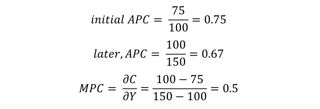
As long as APC falls with an increase in income, MPC will always be less than APC. Since the absolute income hypothesis postulates that APC decreases with an increase in income, MPC will be less than APC.

absolute income hypothesis: consumption function

The consumption function associated with the absolute income hypothesis can be expressed as:

Autonomous consumption is the minimum consumption expenditure even when the real income is zero, i.e. consumers must spend a certain minimum amount. For instance, consumers need to purchase some necessities for survival despite zero income. This kind of consumption may be carried out from previous savings or borrowings.

As income rises, consumption increases as well. The increase in consumption is shown by the slope coefficient (MPC).

Empirical Evidence

Long run consumption.

A study conducted by Simon Kuznets in 1946 showed a different type of consumption expenditure. In the long run, it was observed that on average, APC did not decline with an increase in income. Therefore, APC and MPC were equal even as income grew along the trend. Hence, the consumption function trend was a straight line passing through origin with MPC equal to APC. The Absolute Income Hypothesis could not explain this behaviour.

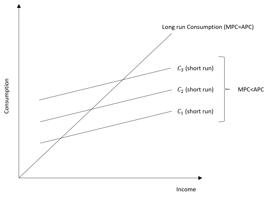
Role of business cycles or cyclical fluctuations

Kuznets also observed that APC was below the trend during periods of a boom in the economy and above the trend during periods of slump. In the short run, therefore, consumption behaved similarly to the propositions of the absolute income hypothesis. This is because APC declined with an increase in income as it was observed to be below trend during the boom (high income) periods in a business cycle. As a result, MPC < APC during the short run due to cyclical fluctuations in income.

Cross-sectional studies

In addition to business cycles, MPC was observed to be less than APC in cross-sectional studies. Hence, APC was observed to decline with an increase in income across different sections of consumers. This implies that consumers with higher incomes tend to spend a relatively smaller proportion of their income.

Based on the above observations, the consumption function put forward by the absolute income hypothesis can be considered a short-run consumption function. This is understandable because the cross-sectional and short-run behaviour of the consumption function was observed to be the same as proposed by the absolute income hypothesis.

criticism of the Absolute Income Hypothesis

• It fails to explain the long-run behaviour of consumption observed by Kuznets, where MPC=APC.
• The theory did not explicitly account for the role of cyclical fluctuations or business cycles, where MPC<APC over a short period only.
• Stagnation thesis and role of wealth:

Based on the absolute income hypothesis, economists believed that economies will stagnate after World War 2. As income rises, consumption will increase but the ratio of consumption expenditure to income ( C / Y ) will go on decreasing. Real output in an economy is a combination of consumption, investment and government expenditure:

As “ C / Y”  falls with a rise in income, either “I / Y” or “G / Y” must increase to maintain the full employment level in the economy. There is no way to determine whether “I / Y” will increase or decrease, therefore, “G / Y” must increase. Hence, government spending must increase at a faster rate than income, otherwise, the economy will stagnate.

After World War 2, government spending would fall and economies would plunge into recession or depression. But, the opposite happened and consumption increased leading to inflation instead of stagnation. This happened because consumer expenditure was controlled through rationing during the war. The extra income during that period was converted into assets or wealth. When the war ended, it led to a jump in consumer expenditure due to the increased assets and wealth. This proved that income is not the only determinant of consumption, but, wealth also plays an important role in consumption expenditure.

Other theories such as the Permanent Income Hypothesis , Relative Income Hypothesis and Life-cycle Hypothesis attempted to overcome the shortcomings of this theory and explain the empirical results.

You Might Also Like

Relative income hypothesis, phillips curve: short run and long run, difference between microeconomics and macroeconomics, leave a reply cancel reply.

To provide the best experiences, we and our partners use technologies like cookies to store and/or access device information. Consenting to these technologies will allow us and our partners to process personal data such as browsing behavior or unique IDs on this site and show (non-) personalized ads. Not consenting or withdrawing consent, may adversely affect certain features and functions.

Click below to consent to the above or make granular choices. Your choices will be applied to this site only. You can change your settings at any time, including withdrawing your consent, by using the toggles on the Cookie Policy, or by clicking on the manage consent button at the bottom of the screen.

Keeping up with the Joneses: macro-evidence on the relevance of Duesenberry’s relative income hypothesis in Ethiopia*

• Research Paper
• Published: 24 May 2022
• Volume 24 , pages 549–564, ( 2022 )

Cite this article

• Tazeb Bisset 1 &
• Dagmawe Tenaw 2  

314 Accesses

Explore all metrics

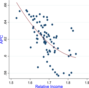
Despite being mysteriously ignored and displaced by mainstream consumption theories, Duesenberry’s relative income hypothesis appears to be highly relevant to modern societies where individuals are becoming increasingly obsessed with their social status. Accordingly, this study aims to provide some evidence on relative income hypothesis by investigating the relevance of Duesenberry’s demonstration and ratchet effects in Ethiopia using quarterly data from 1999/2000Q1 to 2018/19Q4. We estimate two specifications of the relative income hypothesis using the traditional Autoregressive Distributed Lag (ARDL) model and the dynamic ARDL simulations approach. The findings confirm a Backward-J-shaped demonstration effect , implying that an increase in relative income induces a steeper reduction in Average Propensity to Consume (APC) at lower-income groups (the demonstration effect is stronger for lower-income groups). The results also support the ratchet effect , indicating the importance of past consumption habits for current consumption decisions. In resolving the consumption puzzle, the presence of demonstration and ratchet effects reflects a stable APC in the long run. Therefore, consumption-related policies should be carefully designed, as policies aimed at boosting aggregate demand can motivate low-income households to gallop into a wasteful competition to ‘ keep up with the Joneses ’—the relative riches.

This is a preview of subscription content, log in via an institution to check access.

Access this article

Price includes VAT (Russian Federation)

Instant access to the full article PDF.

Rent this article via DeepDyve

Institutional subscriptions

Similar content being viewed by others

The Relationship Between Income Inequality and Economic Growth: Are Transmission Channels Effective?

Does financial inclusion reduce poverty and income inequality in developing countries a panel data analysis.

Money and Happiness: Income, Wealth and Subjective Well-Being

It is relative income, not absolute one, which matters more for consumption decisions of an individual.

Past consumption patterns (habit formation) significantly determines an individual’s current consumption.

Abebe S (2006) Essay on poverty, risk and consumption dynamics in Ethiopia. Doctoral thesis, Goteborg University, School of Business, Economics and Law. http://hdl.handle.net/2077/2908

Alimi RS (2013) Keynes' Absolute Income Hypothesis and Kuznets Paradox

Alimi RS (2015) Estimating consumption function under permanent income hypothesis: a comparison between Nigeria and South Africa. Int J Acad Res Bus Soc Sci. https://doi.org/10.6007/IJARBSS/v5-i11/1917

Article   Google Scholar  

Altunc OF, Aydin C (2014) An estimation of the consumption function under the permanent income hypothesis: the case of D-8 countries. J Econ Cooper Dev 35(3):29–42

Google Scholar  

Bisset T, Tenaw D (2020) Keeping up with the joneses: the relevance of duesenberry’s relative income hypothesis in ethiopia. Research Square. https://doi.org/10.21203/rs.3.rs-83692/v1

Brown TM (1952) Habit persistence and lags in consumer behavior. Econometrica 20(3):355–371. https://doi.org/10.2307/1907409

Davis TE (1952) The consumption function as a tool for prediction. Rev Econ Stat 34(3):270–277. https://doi.org/10.2307/1925635

DeJuan J, SeaterJ WirjantoT (2006) Testing the permanent-income hypothesis new evidence from West-German States. Empir Econ 31:613–629

Douglas M, Isherwood B (1978) The World of Goods: Towards an Archaeology of Consumption

Duesenberry JS (1949) Income, saving and the theory of consumption behavior. Harvard University Press, Cambridge

Duesenberry JS, Eckstein O, Fromm G (1960) A simulation of the United States economy in recession. Econometrica 28(4):749–809. https://doi.org/10.2307/1907563

Easterlin RA (1974) Does economic growth improve the human lot? Some empirical evidence. Nations and Households in Economic Growth: Essays in Honor of Moses Abramovitz. https://doi.org/10.1016/B978-0-12-205050-3.50008-7

Elliott G, Rothenberg TJ, Stock JH (1996) Efficient tests for an autoregressive unit root. Econometrica 64:813−836

Frank RH (1985) The demand for unobservable and other nonpositional goods. The American Economic Review 75(1):101–116

Frank RH (2005) The mysterious disappearance of James Duesenberry. The New York Times

Friedman M (1957) A theory of the consumption function. Princeton University Press, Princeton

Book   Google Scholar  

Gaertner W (1974) A dynamic model of interdependent consumer behavior. Zeitschrift Für Nationalökonomie/journal of Economics 34:327–344

Gomes FAR (2012) A direct test of the permanent income hypothesis: the brazilian case. Brazilian Business Review 9(4):87−102

Gupta R, Ziramba E (2011) Is the permanent income hypothesis really well-suited for forecasting? East Econ J 37:165–177. https://doi.org/10.1057/eej.2010.14

Hamilton D (2001) Comment provoked by Mason´s “Duesenberry´s contribution to consumer theory.” J Econ Issues. https://doi.org/10.1080/00213624.2001.11506400

Jordan S, Philips AQ (2018) Cointegration testing and dynamic simulations of autoregressive distributed lag models. Stata J Promot Commun Stat Stata 18(4):902–923. https://doi.org/10.1177/1536867X1801800409

Kelikume I, Alabi F, Anetor F (2017) Nigeria consumption function—an empirical test of the permanent income hypothesis. J Glob Econ Manag Bus Res 9(1):17–24

Keynes JM (1936) The general theory of employment, interest, and money. Macmillan, London

Khalid K, Mohammed N (2011) Permanent income hypothesis, myopia and liquidity constraints: a case study of Pakistan. Pak J Soc Sci 31(2):299–307

Khan H (2014) An empirical investigation of consumption function under relative income hypothesis: evidence from farm households in Northern Pakistan. Int J Econ Sci 3(2):43–52

Kuznets S (1942) Uses of national income in peace and war. National Bureau of Economic Research, New York

Leibenstein H (1950) Bandwagon, snob and veblen effects in the theory of consumers’ demand. Q J Econ 64(2):183–207. https://doi.org/10.2307/1882692

Mason R (2000) The social significance of consumption: james Duesenberry’s contribution to consumer theory. J Econ Issues 34(3):553–572

McCormick K (1983) Duesenberry and veblen: the demonstration effect revisited. J Econ Issues 17(4):1125–1129

McCormick K (2018) James Duesenberry as a practitioner of behavioral economics. J Behav Econ Policy 2(1):13–18

Modigliani F, Brumberg R (1954) Utility analysis and the consumption function: an interpretation of cross-section data. In: Kurihara KK (ed) Post-Keynesian economics. Rutgers University Press, New Brunswick, pp 388–436

Nkoro E, Uko AK (2016) Autoregressive Distributed Lag (ARDL) cointegration technique: application and interpretation. J Stat Econ Methods 5(4):63–91

Osei-Fosu AK, Butu MM, Osei-Fosu AK (2014) Does Ghanaian’s consumption function follow the permanent income hypothesis? The Cagan’s adaptive expectation approach. Afr Dev Resour Res Inst (Adrri) J133–148

Palley T (2008) The relative income theory of consumption: a synthetic Keynes-Duesenberry-Friedman model. Working paper 170, Political Economy Research Institute

Parada JC, Mejia WB (2009) The relevance of Duesenberry consumption theory: an applied case to Latin America. Revista De Economía Del Caribe 4:19–36

Paz LS (2006) Consumption in Brazil: myopia or liquidity constraints? A simple test using quarterly data. Appl Econ Lett 13(15):961–964. https://doi.org/10.1080/13504850500425931

Pesaran MH, Shin Y, Smith RJ (2001) Bounds testing approaches to the analysis of level relationships. J Appl Econ 16(3):289–326. https://doi.org/10.1002/jae.616

Pollak, R. A. (1976). Interdependent Preferences. The American Economic Review, 66(3): 309–320. https://www.jstor.org/stable/1828165

Reid M (1952) Effect of income concept upon expenditure curves of farm families. In: conference on research in income and wealth, studies in income and wealth, NBER, New York, p 15

Sanders S (2010) A model of the relative income hypothesis. J Econ Educ 41(3):292–305. https://doi.org/10.1080/00220485.2010.486733

Shrestha MB, Bhatta GR (2018) Selecting appropriate methodological framework for time series data analysis. J Finance Data Sci 4:71–89. https://doi.org/10.1016/j.jfds.2017.11.001

Singh B, Kumar RC (1971) The relative income hypothesis-a cross-country analysis. Rev Income Wealth. https://doi.org/10.1111/j.1475-4991.1971.tb00787.x

Singh B, Drost H, Kumar RC (1978) An empirical evaluation of the relative, permanent income and the life-cycle hypothesis. Econ Dev Cultural Change 26(2):281–305

Veblen T (1899) The theory of the leisure class. Macmillan, New York

Download references

Acknowledgements

The authors would like to thank the reviewers for their helpful comments.

No funding was received.

Author information

Authors and affiliations.

Department of Economics, Dire Dawa University, Dire Dawa, Ethiopia

Tazeb Bisset

Department of Economics and Management “Marco Fanno”, University of Padova, Padua, Italy

Dagmawe Tenaw

You can also search for this author in PubMed   Google Scholar

Corresponding author

Correspondence to Tazeb Bisset .

Ethics declarations

Conflict of interest.

The authors declare no competing interest. 

Additional information

Publisher's note.

Springer Nature remains neutral with regard to jurisdictional claims in published maps and institutional affiliations.

The first (preprint) version of this paper is available at Research Square (and can be accessible at www.researchsquare.com/article/rs-83692/v1 ).

Rights and permissions

Reprints and permissions

About this article

Bisset, T., Tenaw, D. Keeping up with the Joneses: macro-evidence on the relevance of Duesenberry’s relative income hypothesis in Ethiopia*. J. Soc. Econ. Dev. 24 , 549–564 (2022). https://doi.org/10.1007/s40847-022-00182-4

Download citation

Accepted : 26 March 2022

Published : 24 May 2022

Issue Date : December 2022

DOI : https://doi.org/10.1007/s40847-022-00182-4

Share this article

Anyone you share the following link with will be able to read this content:

Sorry, a shareable link is not currently available for this article.

Provided by the Springer Nature SharedIt content-sharing initiative

• Duesenberry’s demonstration and ratchet effects
• Relative income
• Consumption puzzle
• Dynamic ARDL simulation
• Find a journal
• Publish with us
• Track your research