example hypothesis for multiple regression

Have a language expert improve your writing

Run a free plagiarism check in 10 minutes, generate accurate citations for free.

• Knowledge Base

Multiple Linear Regression | A Quick Guide (Examples)

Published on February 20, 2020 by Rebecca Bevans . Revised on June 22, 2023.

Regression models are used to describe relationships between variables by fitting a line to the observed data. Regression allows you to estimate how a dependent variable changes as the independent variable(s) change.

Multiple linear regression is used to estimate the relationship between  two or more independent variables and one dependent variable . You can use multiple linear regression when you want to know:

• How strong the relationship is between two or more independent variables and one dependent variable (e.g. how rainfall, temperature, and amount of fertilizer added affect crop growth).
• The value of the dependent variable at a certain value of the independent variables (e.g. the expected yield of a crop at certain levels of rainfall, temperature, and fertilizer addition).

Table of contents

Assumptions of multiple linear regression, how to perform a multiple linear regression, interpreting the results, presenting the results, other interesting articles, frequently asked questions about multiple linear regression.

Multiple linear regression makes all of the same assumptions as simple linear regression :

Homogeneity of variance (homoscedasticity) : the size of the error in our prediction doesn’t change significantly across the values of the independent variable.

Independence of observations : the observations in the dataset were collected using statistically valid sampling methods , and there are no hidden relationships among variables.

In multiple linear regression, it is possible that some of the independent variables are actually correlated with one another, so it is important to check these before developing the regression model. If two independent variables are too highly correlated (r2 > ~0.6), then only one of them should be used in the regression model.

Normality : The data follows a normal distribution .

Linearity : the line of best fit through the data points is a straight line, rather than a curve or some sort of grouping factor.

Here's why students love Scribbr's proofreading services

Discover proofreading & editing

Multiple linear regression formula

The formula for a multiple linear regression is:

• … = do the same for however many independent variables you are testing

To find the best-fit line for each independent variable, multiple linear regression calculates three things:

• The regression coefficients that lead to the smallest overall model error.
• The t statistic of the overall model.
• The associated p value (how likely it is that the t statistic would have occurred by chance if the null hypothesis of no relationship between the independent and dependent variables was true).

It then calculates the t statistic and p value for each regression coefficient in the model.

Multiple linear regression in R

While it is possible to do multiple linear regression by hand, it is much more commonly done via statistical software. We are going to use R for our examples because it is free, powerful, and widely available. Download the sample dataset to try it yourself.

Dataset for multiple linear regression (.csv)

Load the heart.data dataset into your R environment and run the following code:

This code takes the data set heart.data and calculates the effect that the independent variables biking and smoking have on the dependent variable heart disease using the equation for the linear model: lm() .

Learn more by following the full step-by-step guide to linear regression in R .

To view the results of the model, you can use the summary() function:

This function takes the most important parameters from the linear model and puts them into a table that looks like this:

The summary first prints out the formula (‘Call’), then the model residuals (‘Residuals’). If the residuals are roughly centered around zero and with similar spread on either side, as these do ( median 0.03, and min and max around -2 and 2) then the model probably fits the assumption of heteroscedasticity.

Next are the regression coefficients of the model (‘Coefficients’). Row 1 of the coefficients table is labeled (Intercept) – this is the y-intercept of the regression equation. It’s helpful to know the estimated intercept in order to plug it into the regression equation and predict values of the dependent variable:

The most important things to note in this output table are the next two tables – the estimates for the independent variables.

The Estimate column is the estimated effect , also called the regression coefficient or r 2 value. The estimates in the table tell us that for every one percent increase in biking to work there is an associated 0.2 percent decrease in heart disease, and that for every one percent increase in smoking there is an associated .17 percent increase in heart disease.

The Std.error column displays the standard error of the estimate. This number shows how much variation there is around the estimates of the regression coefficient.

The t value column displays the test statistic . Unless otherwise specified, the test statistic used in linear regression is the t value from a two-sided t test . The larger the test statistic, the less likely it is that the results occurred by chance.

The Pr( > | t | ) column shows the p value . This shows how likely the calculated t value would have occurred by chance if the null hypothesis of no effect of the parameter were true.

Because these values are so low ( p < 0.001 in both cases), we can reject the null hypothesis and conclude that both biking to work and smoking both likely influence rates of heart disease.

When reporting your results, include the estimated effect (i.e. the regression coefficient), the standard error of the estimate, and the p value. You should also interpret your numbers to make it clear to your readers what the regression coefficient means.

Visualizing the results in a graph

It can also be helpful to include a graph with your results. Multiple linear regression is somewhat more complicated than simple linear regression, because there are more parameters than will fit on a two-dimensional plot.

However, there are ways to display your results that include the effects of multiple independent variables on the dependent variable, even though only one independent variable can actually be plotted on the x-axis.

Here, we have calculated the predicted values of the dependent variable (heart disease) across the full range of observed values for the percentage of people biking to work.

To include the effect of smoking on the independent variable, we calculated these predicted values while holding smoking constant at the minimum, mean , and maximum observed rates of smoking.

Prevent plagiarism. Run a free check.

If you want to know more about statistics , methodology , or research bias , make sure to check out some of our other articles with explanations and examples.

• Chi square test of independence
• Statistical power
• Descriptive statistics
• Degrees of freedom
• Pearson correlation
• Null hypothesis

Methodology

• Double-blind study
• Case-control study
• Research ethics
• Data collection
• Hypothesis testing
• Structured interviews

Research bias

• Hawthorne effect
• Unconscious bias
• Recall bias
• Halo effect
• Self-serving bias
• Information bias

A regression model is a statistical model that estimates the relationship between one dependent variable and one or more independent variables using a line (or a plane in the case of two or more independent variables).

A regression model can be used when the dependent variable is quantitative, except in the case of logistic regression, where the dependent variable is binary.

Multiple linear regression is a regression model that estimates the relationship between a quantitative dependent variable and two or more independent variables using a straight line.

Linear regression most often uses mean-square error (MSE) to calculate the error of the model. MSE is calculated by:

• measuring the distance of the observed y-values from the predicted y-values at each value of x;
• squaring each of these distances;
• calculating the mean of each of the squared distances.

Linear regression fits a line to the data by finding the regression coefficient that results in the smallest MSE.

Cite this Scribbr article

If you want to cite this source, you can copy and paste the citation or click the “Cite this Scribbr article” button to automatically add the citation to our free Citation Generator.

Bevans, R. (2023, June 22). Multiple Linear Regression | A Quick Guide (Examples). Scribbr. Retrieved April 2, 2024, from https://www.scribbr.com/statistics/multiple-linear-regression/

Is this article helpful?

Rebecca Bevans

Other students also liked, simple linear regression | an easy introduction & examples, an introduction to t tests | definitions, formula and examples, types of variables in research & statistics | examples, what is your plagiarism score.

Save 10% on All AnalystPrep 2024 Study Packages with Coupon Code BLOG10 .

• Payment Plans
• Product List
• Partnerships

• Try Free Trial
• Study Packages
• Levels I, II & III Lifetime Package
• Video Lessons
• Study Notes
• Practice Questions
• Levels II & III Lifetime Package
• About the Exam
• About your Instructor
• Part I Study Packages
• Parts I & II Packages
• Part I & Part II Lifetime Package
• Part II Study Packages
• Exams P & FM Lifetime Package
• Quantitative Questions
• Verbal Questions
• Data Insight Questions
• Live Tutoring
• About your Instructors
• EA Practice Questions
• Data Sufficiency Questions
• Integrated Reasoning Questions

Hypothesis Tests and Confidence Intervals in Multiple Regression

After completing this reading you should be able to:

• Construct, apply, and interpret hypothesis tests and confidence intervals for a single coefficient in a multiple regression.
• Construct, apply, and interpret joint hypothesis tests and confidence intervals for multiple coefficients in a multiple regression.
• Interpret the \(F\)-statistic.
• Interpret tests of a single restriction involving multiple coefficients.
• Interpret confidence sets for multiple coefficients.
• Identify examples of omitted variable bias in multiple regressions.
• Interpret the \({ R }^{ 2 }\) and adjusted \({ R }^{ 2 }\) in a multiple regression.

Hypothesis Tests and Confidence Intervals for a Single Coefficient

This section is about the calculation of the standard error, hypotheses testing, and confidence interval construction for a single regression in a multiple regression equation.

Introduction

In a previous chapter, we looked at simple linear regression where we deal with just one regressor (independent variable). The response (dependent variable) is assumed to be affected by just one independent variable.  M ultiple regression, on the other hand ,  simultaneously considers the influence of multiple explanatory variables on a response variable Y. We may want to establish the confidence interval of one of the independent variables. We may want to evaluate whether any particular independent variable has a significant effect on the dependent variable. Finally, We may also want to establish whether the independent variables as a group have a significant effect on the dependent variable. In this chapter, we delve into ways all this can be achieved.

Hypothesis Tests for a single coefficient

Suppose that we are testing the hypothesis that the true coefficient \({ \beta }_{ j }\) on the \(j\)th regressor takes on some specific value \({ \beta }_{ j,0 }\). Let the alternative hypothesis be two-sided. Therefore, the following is the mathematical expression of the two hypotheses:

$$ { H }_{ 0 }:{ \beta }_{ j }={ \beta }_{ j,0 }\quad vs.\quad { H }_{ 1 }:{ \beta }_{ j }\neq { \beta }_{ j,0 } $$

This expression represents the two-sided alternative. The following are the steps to follow while testing the null hypothesis:

• Computing the coefficient’s standard error.

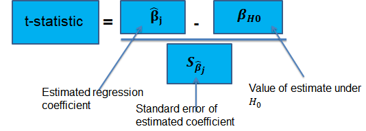
$$ p-value=2\Phi \left( -|{ t }^{ act }| \right) $$

• Also, the \(t\)-statistic can be compared to the critical value corresponding to the significance level that is desired for the test.

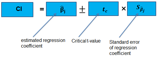
Confidence Intervals for a Single Coefficient

The confidence interval for a regression coefficient in multiple regression is calculated and interpreted the same way as it is in simple linear regression. 

The t-statistic has n – k – 1 degrees of freedom where k = number of independents

Supposing that an interval contains the true value of \({ \beta }_{ j }\) with a probability of 95%. This is simply the 95% two-sided confidence interval for \({ \beta }_{ j }\). The implication here is that the true value of \({ \beta }_{ j }\) is contained in 95% of all possible randomly drawn variables.

Alternatively, the 95% two-sided confidence interval for \({ \beta }_{ j }\) is the set of values that are impossible to reject when a two-sided hypothesis test of 5% is applied. Therefore, with a large sample size:

$$ 95\%\quad confidence\quad interval\quad for\quad { \beta }_{ j }=\left[ { \hat { \beta } }_{ j }-1.96SE\left( { \hat { \beta } }_{ j } \right) ,{ \hat { \beta } }_{ j }+1.96SE\left( { \hat { \beta } }_{ j } \right) \right] $$

Tests of Joint Hypotheses

In this section, we consider the formulation of the joint hypotheses on multiple regression coefficients. We will further study the application of an \(F\)-statistic in their testing.

Hypotheses Testing on Two or More Coefficients

Joint null hypothesis.

In multiple regression, we canno t test the null hypothesis that all slope coefficients are equal 0 based on t -tests that each individual slope coefficient equals 0. Why? individual t-tests do not account for the effects of interactions among the independent variables.

For this reason, we conduct the F-test which uses the F-statistic .  The F-test tests the null hypothesis that all of the slope coefficients in the multiple regression model are jointly equal to 0, .i.e.,

\(F\)-Statistic

The F-statistic, which is always a one-tailed test , is calculated as:

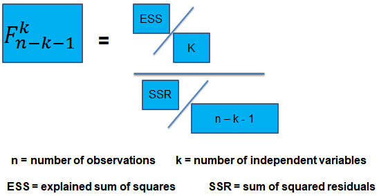
To determine whether at least one of the coefficients is statistically significant, the calculated F-statistic is compared with the one-tailed critical F-value, at the appropriate level of significance.

Decision rule:

Rejection of the null hypothesis at a stated level of significance indicates that at least one of the coefficients is significantly different than zero, i.e, at least one of the independent variables in the regression model makes a significant contribution to the dependent variable.

An analyst runs a regression of monthly value-stock returns on four independent variables over 48 months.

The total sum of squares for the regression is 360, and the sum of squared errors is 120.

Test the null hypothesis at the 5% significance level (95% confidence) that all the four independent variables are equal to zero.

\({ H }_{ 0 }:{ \beta }_{ 1 }=0,{ \beta }_{ 2 }=0,\dots ,{ \beta }_{ 4 }=0 \)

\({ H }_{ 1 }:{ \beta }_{ j }\neq 0\) (at least one j is not equal to zero, j=1,2… k )

ESS = TSS – SSR = 360 – 120 = 240

The calculated test statistic = (ESS/k)/(SSR/(n-k-1))

=(240/4)/(120/43) = 21.5

\({ F }_{ 43 }^{ 4 }\) is approximately 2.44 at 5% significance level.

Decision: Reject H 0 .

Conclusion: at least one of the 4 independents is significantly different than zero.

Omitted Variable Bias in Multiple Regression

This is the bias in the OLS estimator arising when at least one included regressor gets collaborated with an omitted variable. The following conditions must be satisfied for an omitted variable bias to occur:

• There must be a correlation between at least one of the included regressors and the omitted variable.
• The dependent variable \(Y\) must be determined by the omitted variable.

Practical Interpretation of the \({ R }^{ 2 }\) and the adjusted \({ R }^{ 2 }\), \({ \bar { R } }^{ 2 }\)

To determine the accuracy within which the OLS regression line fits the data, we apply the coefficient of determination and the regression’s standard error . 

The coefficient of determination, represented by \({ R }^{ 2 }\), is a measure of the “goodness of fit” of the regression. It is interpreted as the percentage of variation in the dependent variable explained by the independent variables

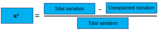
\({ R }^{ 2 }\) is not a reliable indicator of the explanatory power of a multiple regression model.Why? \({ R }^{ 2 }\) almost always increases as new independent variables are added to the model, even if the marginal contribution of the new variable is not statistically significant. Thus, a high \({ R }^{ 2 }\) may reflect the impact of a large set of independents rather than how well the set explains the dependent.This problem is solved by the use of the adjusted \({ R }^{ 2 }\) (extensively covered in chapter 8)

The following are the factors to watch out when guarding against applying the \({ R }^{ 2 }\) or the \({ \bar { R } }^{ 2 }\):

• An added variable doesn’t have to be statistically significant just because the \({ R }^{ 2 }\) or the \({ \bar { R } }^{ 2 }\) has increased.
• It is not always true that the regressors are a true cause of the dependent variable, just because there is a high \({ R }^{ 2 }\) or \({ \bar { R } }^{ 2 }\).
• It is not necessary that there is no omitted variable bias just because we have a high \({ R }^{ 2 }\) or \({ \bar { R } }^{ 2 }\).
• It is not necessarily true that we have the most appropriate set of regressors just because we have a high \({ R }^{ 2 }\) or \({ \bar { R } }^{ 2 }\).
• It is not necessarily true that we have an inappropriate set of regressors just because we have a low \({ R }^{ 2 }\) or \({ \bar { R } }^{ 2 }\).

An economist tests the hypothesis that GDP growth in a certain country can be explained by interest rates and inflation.

Using some 30 observations, the analyst formulates the following regression equation:

$$ GDP growth = { \hat { \beta } }_{ 0 } + { \hat { \beta } }_{ 1 } Interest+ { \hat { \beta } }_{ 2 } Inflation $$

Regression estimates are as follows:

Is the coefficient for interest rates significant at 5%?

• Since the test statistic < t-critical, we accept H 0 ; the interest rate coefficient is  not   significant at the 5% level.
• Since the test statistic > t-critical, we reject H 0 ; the interest rate coefficient is not significant at the 5% level.
• Since the test statistic > t-critical, we reject H 0 ; the interest rate coefficient is significant at the 5% level.
• Since the test statistic < t-critical, we accept H 1 ; the interest rate coefficient is significant at the 5% level.

The correct answer is  C .

We have GDP growth = 0.10 + 0.20(Int) + 0.15(Inf)

Hypothesis:

$$ { H }_{ 0 }:{ \hat { \beta } }_{ 1 } = 0 \quad vs \quad { H }_{ 1 }:{ \hat { \beta } }_{ 1 }≠0 $$

The test statistic is:

$$ t = \left( \frac { 0.20 – 0 }{ 0.05 } \right)  = 4 $$

The critical value is t (α/2, n-k-1) = t 0.025,27  = 2.052 (which can be found on the t-table).

Conclusion : The interest rate coefficient is significant at the 5% level.

Offered by AnalystPrep

Modeling Cycles: MA, AR, and ARMA Models

Empirical approaches to risk metrics and hedging, multifactor models of risk-adjusted as ....

After completing this reading, you should be able to: Explain the arbitrage pricing... Read More

The Black-Scholes-Merton Model

After completing this reading you should be able to: Explain the lognormal property... Read More

Exchanges and OTC Markets

After completing this reading, you should be able to: Describe how exchanges can... Read More

Properties of Options

After completing this reading, you should be able to: Identify the six factors... Read More

Leave a Comment Cancel reply

You must be logged in to post a comment.

Want to create or adapt books like this? Learn more about how Pressbooks supports open publishing practices.

Section 5.3: Multiple Regression Explanation, Assumptions, Interpretation, and Write Up

Learning Objectives

At the end of this section you should be able to answer the following questions:

• Explain the difference between Multiple Regression and Simple Regression.
• Explain the assumptions underlying Multiple Regression.

Multiple Regression is a step beyond simple regression. The main difference between simple and multiple regression is that multiple regression includes two or more independent variables – sometimes called predictor variables – in the model, rather than just one.

As such, the purpose of multiple regression is to determine the utility of a set of predictor variables for predicting an outcome, which is generally some important event or behaviour. This outcome can be designated as the outcome variable, the dependent variable, or the criterion variable. For example, you might hypothesise that the need to belong will predict motivations for Facebook use and that self-esteem and meaningful existence will uniquely predict motivations for Facebook use.

Before beginning your analysis, you should consider the following points:

• Regression analyses reveal relationships among variables (relationship between the criterion variable and the linear combination of a set of predictor variables) but do not imply a causal relationship.
• A regression solution – or set of predictor variables – is sensitive to combinations of variables. Whether a predictor is important in a solution depends on the other predictors in the set. If the predictor of interest is the only one that assesses some important facet of the outcome, it will appear important. If a predictor is only one of several predictors that assess the same important facet of the outcome, it will appear less important.  For a good set of predictor variables – the smallest set of uncorrelated variables is best.

PowerPoint: Venn Diagrams

Please click on the link labeled “Venn Diagrams” to work through an example.

• Chapter Five – Venn Diagrams

In these Venn Diagrams, you can see why it is best for the predictors to be strongly correlated with the dependent variable but uncorrelated with the other Independent Variables. This reduces the amount of shared variance between the independent variables.  The illustration in Slide 2 shows logical relationships between predictors, for two different possible regression models in separate Venn diagrams. On the left, you can see three partially correlated independent variables on a single dependent variable. The three partially correlated independent variables are physical health, mental health, and spiritual health and the dependent variable is life satisfaction. On the right, you have three highly correlated independent variables (e.g., BMI, blood pressure, heart rate) on the dependent variable of life satisfaction. The model on the left would have some use in discovering the associations between those variables, however, the model on the right would not be useful, as all three of the independent variables are basically measuring the same thing and are mostly accounting for the same variability in the dependent variable.

There are two main types of regression with multiple independent variables:

• Standard or Single Step: Where all predictors enter the regression together.
• Sequential or Hierarchical:  Where all predictors are entered in blocks. Each block represents one step.

We will now be exploring the single step multiple regression:

All predictors enter the regression equation at once. Each predictor is treated as if it had been analysed in the regression model after all other predictors had been analysed. These predictors are evaluated by the shared variance (i.e., level of prediction) shared between the dependant variable and the individual predictor variable.

Multiple Regression Assumptions

There are a number of assumptions that should be assessed before performing a multiple regression analysis:

• The dependant variable (the variable of interest) needs to be using a continuous scale.
• There are two or more independent variables. These can be measured using either continuous or categorical means.
• The three or more variables of interest should have a linear relationship, which you can check by using a scatterplot.
• The data should have homoscedasticity. In other words, the line of best fit is not dissimilar as the data points move across the line in a positive or negative direction. Homoscedasticity can be checked by producing standardised residual plots against the unstandardized predicted values.
• The data should not have two or more independent variables that are highly correlated. This is called multicollinearity which can be checked using Variance-inflation-factor or VIF values. High VIF indicates that the associated independent variable is highly collinear with the other variables in the model.
• There should be no spurious outliers.
• The residuals (errors) should be approximately normally distributed. This can be checked by a histogram (with a superimposed normal curve) and by plotting the of the standardised residuals using either a P-P Plot, or a Normal Q-Q Plot .

Multiple Regression Interpretation

For our example research question, we will be looking at the combined effect of three predictor variables – perceived life stress, location, and age – on the outcome variable of physical health?  

PowerPoint: Standard Regression

Please open the output at the link labeled “Chapter Five – Standard Regression” to view the output.

• Chapter Five – Standard Regression

Slide 1 contains the standard regression analysis output.

On Slide 2 you can see in the red circle, the test statistics are significant.  The F-statistic examines the overall significance of the model, and shows if your predictors as a group provide a better fit to the data than no predictor variables, which they do in this example.

The R 2 values are shown in the green circle. The R 2 value shows the total amount of variance accounted for in the criterion by the predictors, and the adjusted R 2 is the estimated value of  R 2 in the population.  

Moving on to the individual variable effects on Slide 3, you can see the significance of the contribution of individual predictors in light blue. The unstandardized slope or the B value is shown in red, which represents the change caused by the variable (e.g., increasing  1 unit of perceived stress will raise physical illness by .40). Finally, you can see the standardised slope value in green, which are also known as beta values. These values are standardised ranging from +/-0 to 1, similar to an r value.  

We should also briefly discuss dummy variables:

A dummy variable is a variable that is used to represent categorical information relating to the participants in a study. This could include gender, location, race, age groups, and you get the idea.  Dummy variables are most often represented as dichotomous variables (they only have two values). When performing a regression, it is easier for interpretation if the values for the dummy variable is set to 0 or 1. 1 usually resents when a characteristic is present. For example, a question asking the participants “Do you have a drivers license” with a forced choice response of yes or no.

In this example on Slide 3 and circled in red, the variable is gender with male = 0, and female = 1. A positive Beta (B) means an association with 1, whereas a negative beta means an association with 0. In this case, being female was associated with greater levels of physical illness.

Multiple Regression Write Up

Here is an example of how to write up the results of a standard multiple regression analysis:

In order to test the research question, a multiple regression was conducted, with age, gender (0 = male, 1 = female), and perceived life stress as the predictors, with levels of physical illness as the dependent variable. Overall, the results showed the utility of the predictive model was significant, F (3,363) = 39.61, R 2 = .25, p < .001. All of the predictors explain a large amount of the variance between the variables (25%).  The results showed that perceived stress and gender of participants were significant positive predictors of physical illness ( β =.47, t = 9.96, p < .001, and β =.15, t = 3.23, p = .001, respectively). The results showed that age ( β =-.02, t = -0.49 p = .63) was not a significant predictor of perceived stress.

Statistics for Research Students Copyright © 2022 by University of Southern Queensland is licensed under a Creative Commons Attribution 4.0 International License , except where otherwise noted.

Share This Book

Multiple linear regression

Multiple linear regression #.

Fig. 11 Multiple linear regression #

Errors: \(\varepsilon_i \sim N(0,\sigma^2)\quad \text{i.i.d.}\)

Fit: the estimates \(\hat\beta_0\) and \(\hat\beta_1\) are chosen to minimize the residual sum of squares (RSS):

Matrix notation: with \(\beta=(\beta_0,\dots,\beta_p)\) and \({X}\) our usual data matrix with an extra column of ones on the left to account for the intercept, we can write

Multiple linear regression answers several questions #

Is at least one of the variables \(X_i\) useful for predicting the outcome \(Y\) ?

Which subset of the predictors is most important?

How good is a linear model for these data?

Given a set of predictor values, what is a likely value for \(Y\) , and how accurate is this prediction?

The estimates \(\hat\beta\) #

Our goal again is to minimize the RSS: $ \( \begin{aligned} \text{RSS}(\beta) &= \sum_{i=1}^n (y_i -\hat y_i(\beta))^2 \\ & = \sum_{i=1}^n (y_i - \beta_0- \beta_1 x_{i,1}-\dots-\beta_p x_{i,p})^2 \\ &= \|Y-X\beta\|^2_2 \end{aligned} \) $

One can show that this is minimized by the vector \(\hat\beta\) : $ \(\hat\beta = ({X}^T{X})^{-1}{X}^T{y}.\) $

We usually write \(RSS=RSS(\hat{\beta})\) for the minimized RSS.

Which variables are important? #

Consider the hypothesis: \(H_0:\) the last \(q\) predictors have no relation with \(Y\) .

Based on our model: \(H_0:\beta_{p-q+1}=\beta_{p-q+2}=\dots=\beta_p=0.\)

Let \(\text{RSS}_0\) be the minimized residual sum of squares for the model which excludes these variables.

The \(F\) -statistic is defined by: $ \(F = \frac{(\text{RSS}_0-\text{RSS})/q}{\text{RSS}/(n-p-1)}.\) $

Under the null hypothesis (of our model), this has an \(F\) -distribution.

Example: If \(q=p\) , we test whether any of the variables is important. $ \(\text{RSS}_0 = \sum_{i=1}^n(y_i-\overline y)^2 \) $

The \(t\) -statistic associated to the \(i\) th predictor is the square root of the \(F\) -statistic for the null hypothesis which sets only \(\beta_i=0\) .

A low \(p\) -value indicates that the predictor is important.

Warning: If there are many predictors, even under the null hypothesis, some of the \(t\) -tests will have low p-values even when the model has no explanatory power.

How many variables are important? #

When we select a subset of the predictors, we have \(2^p\) choices.

A way to simplify the choice is to define a range of models with an increasing number of variables, then select the best.

Forward selection: Starting from a null model, include variables one at a time, minimizing the RSS at each step.

Backward selection: Starting from the full model, eliminate variables one at a time, choosing the one with the largest p-value at each step.

Mixed selection: Starting from some model, include variables one at a time, minimizing the RSS at each step. If the p-value for some variable goes beyond a threshold, eliminate that variable.

Choosing one model in the range produced is a form of tuning . This tuning can invalidate some of our methods like hypothesis tests and confidence intervals…

How good are the predictions? #

The function predict in R outputs predictions and confidence intervals from a linear model:

Prediction intervals reflect uncertainty on \(\hat\beta\) and the irreducible error \(\varepsilon\) as well.

These functions rely on our linear regression model $ \( Y = X\beta + \epsilon. \) $

Dealing with categorical or qualitative predictors #

For each qualitative predictor, e.g. Region :

Choose a baseline category, e.g. East

For every other category, define a new predictor:

\(X_\text{South}\) is 1 if the person is from the South region and 0 otherwise

\(X_\text{West}\) is 1 if the person is from the West region and 0 otherwise.

The model will be: $ \(Y = \beta_0 + \beta_1 X_1 +\dots +\beta_7 X_7 + \color{Red}{\beta_\text{South}} X_\text{South} + \beta_\text{West} X_\text{West} +\varepsilon.\) $

The parameter \(\color{Red}{\beta_\text{South}}\) is the relative effect on Balance (our \(Y\) ) for being from the South compared to the baseline category (East).

The model fit and predictions are independent of the choice of the baseline category.

However, hypothesis tests derived from these variables are affected by the choice.

Solution: To check whether region is important, use an \(F\) -test for the hypothesis \(\beta_\text{South}=\beta_\text{West}=0\) by dropping Region from the model. This does not depend on the coding.

Note that there are other ways to encode qualitative predictors produce the same fit \(\hat f\) , but the coefficients have different interpretations.

So far, we have:

Defined Multiple Linear Regression

Discussed how to test the importance of variables.

Described one approach to choose a subset of variables.

Explained how to code qualitative variables.

Now, how do we evaluate model fit? Is the linear model any good? What can go wrong?

How good is the fit? #

To assess the fit, we focus on the residuals $ \( e = Y - \hat{Y} \) $

The RSS always decreases as we add more variables.

The residual standard error (RSE) corrects this: $ \(\text{RSE} = \sqrt{\frac{1}{n-p-1}\text{RSS}}.\) $

Fig. 12 Residuals #

Visualizing the residuals can reveal phenomena that are not accounted for by the model; eg. synergies or interactions:

Potential issues in linear regression #

Interactions between predictors

Non-linear relationships

Correlation of error terms

Non-constant variance of error (heteroskedasticity)

High leverage points

Collinearity

Interactions between predictors #

Linear regression has an additive assumption: $ \(\mathtt{sales} = \beta_0 + \beta_1\times\mathtt{tv}+ \beta_2\times\mathtt{radio}+\varepsilon\) $

i.e. An increase of 100 USD dollars in TV ads causes a fixed increase of \(100 \beta_2\) USD in sales on average, regardless of how much you spend on radio ads.

We saw that in Fig 3.5 above. If we visualize the fit and the observed points, we see they are not evenly scattered around the plane. This could be caused by an interaction.

One way to deal with this is to include multiplicative variables in the model:

The interaction variable tv \(\cdot\) radio is high when both tv and radio are high.

R makes it easy to include interaction variables in the model:

Non-linearities #

Fig. 13 A nonlinear fit might be better here. #

Example: Auto dataset.

A scatterplot between a predictor and the response may reveal a non-linear relationship.

Solution: include polynomial terms in the model.

Could use other functions besides polynomials…

Fig. 14 Residuals for Auto data #

In 2 or 3 dimensions, this is easy to visualize. What do we do when we have too many predictors?

Correlation of error terms #

We assumed that the errors for each sample are independent:

What if this breaks down?

The main effect is that this invalidates any assertions about Standard Errors, confidence intervals, and hypothesis tests…

Example : Suppose that by accident, we duplicate the data (we use each sample twice). Then, the standard errors would be artificially smaller by a factor of \(\sqrt{2}\) .

When could this happen in real life:

Time series: Each sample corresponds to a different point in time. The errors for samples that are close in time are correlated.

Spatial data: Each sample corresponds to a different location in space.

Grouped data: Imagine a study on predicting height from weight at birth. If some of the subjects in the study are in the same family, their shared environment could make them deviate from \(f(x)\) in similar ways.

Correlated errors #

Simulations of time series with increasing correlations between \(\varepsilon_i\)

Non-constant variance of error (heteroskedasticity) #

The variance of the error depends on some characteristics of the input features.

To diagnose this, we can plot residuals vs. fitted values:

If the trend in variance is relatively simple, we can transform the response using a logarithm, for example.

Outliers from a model are points with very high errors.

While they may not affect the fit, they might affect our assessment of model quality.

Possible solutions: #

If we believe an outlier is due to an error in data collection, we can remove it.

An outlier might be evidence of a missing predictor, or the need to specify a more complex model.

High leverage points #

Some samples with extreme inputs have an outsized effect on \(\hat \beta\) .

This can be measured with the leverage statistic or self influence :

Studentized residuals #

The residual \(e_i = y_i - \hat y_i\) is an estimate for the noise \(\epsilon_i\) .

The standard error of \(\hat \epsilon_i\) is \(\sigma \sqrt{1-h_{ii}}\) .

A studentized residual is \(\hat \epsilon_i\) divided by its standard error (with appropriate estimate of \(\sigma\) )

When model is correct, it follows a Student-t distribution with \(n-p-2\) degrees of freedom.

Collinearity #

Two predictors are collinear if one explains the other well:

Problem: The coefficients become unidentifiable .

Consider the extreme case of using two identical predictors limit : $ \( \begin{aligned} \mathtt{balance} &= \beta_0 + \beta_1\times\mathtt{limit} + \beta_2\times\mathtt{limit} + \epsilon \\ & = \beta_0 + (\beta_1+100)\times\mathtt{limit} + (\beta_2-100)\times\mathtt{limit} + \epsilon \end{aligned} \) $

For every \((\beta_0,\beta_1,\beta_2)\) the fit at \((\beta_0,\beta_1,\beta_2)\) is just as good as at \((\beta_0,\beta_1+100,\beta_2-100)\) .

If 2 variables are collinear, we can easily diagnose this using their correlation.

A group of \(q\) variables is multilinear if these variables “contain less information” than \(q\) independent variables.

Pairwise correlations may not reveal multilinear variables.

The Variance Inflation Factor (VIF) measures how predictable it is given the other variables, a proxy for how necessary a variable is:

Above, \(R^2_{X_j|X_{-j}}\) is the \(R^2\) statistic for Multiple Linear regression of the predictor \(X_j\) onto the remaining predictors.

• school Campus Bookshelves
• menu_book Bookshelves
• perm_media Learning Objects
• login Login
• how_to_reg Request Instructor Account
• hub Instructor Commons
• Download Page (PDF)
• Download Full Book (PDF)
• Periodic Table
• Physics Constants
• Scientific Calculator
• Reference & Cite
• Tools expand_more
• Readability

selected template will load here

This action is not available.

14.8: Introduction to Multiple Regression

• Last updated
• Save as PDF
• Page ID 2648

• Rice University

Learning Objectives

• State the regression equation
• Define "regression coefficient"
• Define "beta weight"
• Explain what \(R\) is and how it is related to \(r\)
• Explain why a regression weight is called a "partial slope"
• Explain why the sum of squares explained in a multiple regression model is usually less than the sum of the sums of squares in simple regression
• Define \(R^2\) in terms of proportion explained
• Test \(R^2\) for significance
• Test the difference between a complete and reduced model for significance
• State the assumptions of multiple regression and specify which aspects of the analysis require assumptions

In simple linear regression, a criterion variable is predicted from one predictor variable. In multiple regression, the criterion is predicted by two or more variables. For example, in the SAT case study, you might want to predict a student's university grade point average on the basis of their High-School GPA (\(HSGPA\)) and their total SAT score (verbal + math). The basic idea is to find a linear combination of \(HSGPA\) and \(SAT\) that best predicts University GPA (\(UGPA\)). That is, the problem is to find the values of \(b_1\) and \(b_2\) in the equation shown below that give the best predictions of \(UGPA\). As in the case of simple linear regression, we define the best predictions as the predictions that minimize the squared errors of prediction.

\[UGPA' = b_1HSGPA + b_2SAT + A\]

where \(UGPA'\) is the predicted value of University GPA and \(A\) is a constant. For these data, the best prediction equation is shown below:

\[UGPA' = 0.541 \times HSGPA + 0.008 \times SAT + 0.540\]

In other words, to compute the prediction of a student's University GPA, you add up their High-School GPA multiplied by \(0.541\), their \(SAT\) multiplied by \(0.008\), and \(0.540\). Table \(\PageIndex{1}\) shows the data and predictions for the first five students in the dataset.

The values of \(b\) (\(b_1\) and \(b_2\)) are sometimes called "regression coefficients" and sometimes called "regression weights." These two terms are synonymous.

The multiple correlation (\(R\)) is equal to the correlation between the predicted scores and the actual scores. In this example, it is the correlation between \(UGPA'\) and \(UGPA\), which turns out to be \(0.79\). That is, \(R = 0.79\). Note that \(R\) will never be negative since if there are negative correlations between the predictor variables and the criterion, the regression weights will be negative so that the correlation between the predicted and actual scores will be positive.

Interpretation of Regression Coefficients

A regression coefficient in multiple regression is the slope of the linear relationship between the criterion variable and the part of a predictor variable that is independent of all other predictor variables. In this example, the regression coefficient for \(HSGPA\) can be computed by first predicting \(HSGPA\) from \(SAT\) and saving the errors of prediction (the differences between \(HSGPA\) and \(HSGPA'\)). These errors of prediction are called "residuals" since they are what is left over in \(HSGPA\) after the predictions from \(SAT\) are subtracted, and represent the part of \(HSGPA\) that is independent of \(SAT\). These residuals are referred to as \(HSGPA.SAT\), which means they are the residuals in \(HSGPA\) after having been predicted by \(SAT\). The correlation between \(HSGPA.SAT\) and \(SAT\) is necessarily \(0\).

The final step in computing the regression coefficient is to find the slope of the relationship between these residuals and \(UGPA\). This slope is the regression coefficient for \(HSGPA\). The following equation is used to predict \(HSGPA\) from \(SAT\):

\[HSGPA' = -1.314 + 0.0036 \times SAT\]

The residuals are then computed as:

\[HSGPA - HSGPA'\]

The linear regression equation for the prediction of \(UGPA\) by the residuals is

\[UGPA' = 0.541 \times HSGPA.SAT + 3.173\]

Notice that the slope (\(0.541\)) is the same value given previously for \(b_1\) in the multiple regression equation.

This means that the regression coefficient for \(HSGPA\) is the slope of the relationship between the criterion variable and the part of \(HSGPA\) that is independent of (uncorrelated with) the other predictor variables. It represents the change in the criterion variable associated with a change of one in the predictor variable when all other predictor variables are held constant. Since the regression coefficient for \(HSGPA\) is \(0.54\), this means that, holding \(SAT\) constant, a change of one in \(HSGPA\) is associated with a change of \(0.54\) in \(UGPA'\). If two students had the same \(SAT\) and differed in \(HSGPA\) by \(2\), then you would predict they would differ in \(UGPA\) by \((2)(0.54) = 1.08\). Similarly, if they differed by \(0.5\), then you would predict they would differ by \((0.50)(0.54) = 0.27\).

The slope of the relationship between the part of a predictor variable independent of other predictor variables and the criterion is its partial slope. Thus the regression coefficient of \(0.541\) for \(HSGPA\) and the regression coefficient of \(0.008\) for \(SAT\) are partial slopes. Each partial slope represents the relationship between the predictor variable and the criterion holding constant all of the other predictor variables.

It is difficult to compare the coefficients for different variables directly because they are measured on different scales. A difference of \(1\) in \(HSGPA\) is a fairly large difference, whereas a difference of \(1\) on the \(SAT\) is negligible. Therefore, it can be advantageous to transform the variables so that they are on the same scale. The most straightforward approach is to standardize the variables so that they each have a standard deviation of \(1\). A regression weight for standardized variables is called a "beta weight" and is designated by the Greek letter \(β\). For these data, the beta weights are \(0.625\) and \(0.198\). These values represent the change in the criterion (in standard deviations) associated with a change of one standard deviation on a predictor [holding constant the value(s) on the other predictor(s)]. Clearly, a change of one standard deviation on \(HSGPA\) is associated with a larger difference than a change of one standard deviation of \(SAT\). In practical terms, this means that if you know a student's \(HSGPA\), knowing the student's \(SAT\) does not aid the prediction of \(UGPA\) much. However, if you do not know the student's \(HSGPA\), his or her \(SAT\) can aid in the prediction since the \(β\) weight in the simple regression predicting \(UGPA\) from \(SAT\) is \(0.68\). For comparison purposes, the \(β\) weight in the simple regression predicting \(UGPA\) from \(HSGPA\) is \(0.78\). As is typically the case, the partial slopes are smaller than the slopes in simple regression.

Partitioning the Sums of Squares

Just as in the case of simple linear regression, the sum of squares for the criterion (\(UGPA\) in this example) can be partitioned into the sum of squares predicted and the sum of squares error. That is,

\[SSY = SSY' + SSE\]

which for these data:

\[20.798 = 12.961 + 7.837\]

The sum of squares predicted is also referred to as the "sum of squares explained." Again, as in the case of simple regression,

\[\text{Proportion Explained} = SSY'/SSY\]

In simple regression, the proportion of variance explained is equal to \(r^2\); in multiple regression, the proportion of variance explained is equal to \(R^2\).

In multiple regression, it is often informative to partition the sum of squares explained among the predictor variables. For example, the sum of squares explained for these data is \(12.96\). How is this value divided between \(HSGPA\) and \(SAT\)? One approach that, as will be seen, does not work is to predict \(UGPA\) in separate simple regressions for \(HSGPA\) and \(SAT\). As can be seen in Table \(\PageIndex{2}\), the sum of squares in these separate simple regressions is \(12.64\) for \(HSGPA\) and \(9.75\) for \(SAT\). If we add these two sums of squares we get \(22.39\), a value much larger than the sum of squares explained of \(12.96\) in the multiple regression analysis. The explanation is that \(HSGPA\) and \(SAT\) are highly correlated (\(r = 0.78\)) and therefore much of the variance in \(UGPA\) is confounded between \(HSGPA\) and \(SAT\). That is, it could be explained by either \(HSGPA\) or \(SAT\) and is counted twice if the sums of squares for \(HSGPA\) and \(SAT\) are simply added.

Table \(\PageIndex{3}\) shows the partitioning of the sum of squares into the sum of squares uniquely explained by each predictor variable, the sum of squares confounded between the two predictor variables, and the sum of squares error. It is clear from this table that most of the sum of squares explained is confounded between \(HSGPA\) and \(SAT\). Note that the sum of squares uniquely explained by a predictor variable is analogous to the partial slope of the variable in that both involve the relationship between the variable and the criterion with the other variable(s) controlled.

The sum of squares uniquely attributable to a variable is computed by comparing two regression models: the complete model and a reduced model. The complete model is the multiple regression with all the predictor variables included (\(HSGPA\) and \(SAT\) in this example). A reduced model is a model that leaves out one of the predictor variables. The sum of squares uniquely attributable to a variable is the sum of squares for the complete model minus the sum of squares for the reduced model in which the variable of interest is omitted. As shown in Table \(\PageIndex{2}\), the sum of squares for the complete model (\(HSGPA\) and \(SAT\)) is \(12.96\). The sum of squares for the reduced model in which \(HSGPA\) is omitted is simply the sum of squares explained using \(SAT\) as the predictor variable and is \(9.75\). Therefore, the sum of squares uniquely attributable to \(HSGPA\) is \(12.96 - 9.75 = 3.21\). Similarly, the sum of squares uniquely attributable to \(SAT\) is \(12.96 - 12.64 = 0.32\). The confounded sum of squares in this example is computed by subtracting the sum of squares uniquely attributable to the predictor variables from the sum of squares for the complete model: \(12.96 - 3.21 - 0.32 = 9.43\). The computation of the confounded sums of squares in analysis with more than two predictors is more complex and beyond the scope of this text.

Since the variance is simply the sum of squares divided by the degrees of freedom, it is possible to refer to the proportion of variance explained in the same way as the proportion of the sum of squares explained. It is slightly more common to refer to the proportion of variance explained than the proportion of the sum of squares explained and, therefore, that terminology will be adopted frequently here.

When variables are highly correlated, the variance explained uniquely by the individual variables can be small even though the variance explained by the variables taken together is large. For example, although the proportions of variance explained uniquely by \(HSGPA\) and \(SAT\) are only \(0.15\) and \(0.02\) respectively, together these two variables explain \(0.62\) of the variance. Therefore, you could easily underestimate the importance of variables if only the variance explained uniquely by each variable is considered. Consequently, it is often useful to consider a set of related variables. For example, assume you were interested in predicting job performance from a large number of variables some of which reflect cognitive ability. It is likely that these measures of cognitive ability would be highly correlated among themselves and therefore no one of them would explain much of the variance independently of the other variables. However, you could avoid this problem by determining the proportion of variance explained by all of the cognitive ability variables considered together as a set. The variance explained by the set would include all the variance explained uniquely by the variables in the set as well as all the variance confounded among variables in the set. It would not include variance confounded with variables outside the set. In short, you would be computing the variance explained by the set of variables that is independent of the variables not in the set.

Inferential Statistics

We begin by presenting the formula for testing the significance of the contribution of a set of variables. We will then show how special cases of this formula can be used to test the significance of \(R^2\) as well as to test the significance of the unique contribution of individual variables.

The first step is to compute two regression analyses:

• an analysis in which all the predictor variables are included and
• an analysis in which the variables in the set of variables being tested are excluded.

The former regression model is called the "complete model" and the latter is called the "reduced model." The basic idea is that if the reduced model explains much less than the complete model, then the set of variables excluded from the reduced model is important.

The formula for testing the contribution of a group of variables is:

\[F=\cfrac{\cfrac{SSQ_C-SSQ_R}{p_C-p_R}}{\cfrac{SSQ_T-SSQ_C}{N-p_C-1}}=\cfrac{MS_{explained}}{MS_{error}}\]

\(SSQ_C\) is the sum of squares for the complete model,

\(SSQ_R\) is the sum of squares for the reduced model,

\(p_C\) is the number of predictors in the complete model,

\(p_R\) is the number of predictors in the reduced model,

\(SSQ_T\) is the sum of squares total (the sum of squared deviations of the criterion variable from its mean), and

\(N\) is the total number of observations

The degrees of freedom for the numerator is \(p_C - p_R\) and the degrees of freedom for the denominator is \(N - p_C -1\). If the \(F\) is significant, then it can be concluded that the variables excluded in the reduced set contribute to the prediction of the criterion variable independently of the other variables.

This formula can be used to test the significance of \(R^2\) by defining the reduced model as having no predictor variables. In this application, \(SSQ_R\) and \(p_R = 0\). The formula is then simplified as follows:

\[F=\cfrac{\cfrac{SSQ_C}{p_C}}{\cfrac{SSQ_T-SSQ_C}{N-p_C-1}}=\cfrac{MS_{explained}}{MS_{error}}\]

which for this example becomes:

\[F=\cfrac{\cfrac{12.96}{2}}{\cfrac{20.80-12.96}{105-2-1}}=\cfrac{6.48}{0.08}=84.35\]

The degrees of freedom are \(2\) and \(102\). The \(F\) distribution calculator shows that \(p < 0.001\).

F Calculator

The reduced model used to test the variance explained uniquely by a single predictor consists of all the variables except the predictor variable in question. For example, the reduced model for a test of the unique contribution of \(HSGPA\) contains only the variable \(SAT\). Therefore, the sum of squares for the reduced model is the sum of squares when \(UGPA\) is predicted by \(SAT\). This sum of squares is \(9.75\). The calculations for \(F\) are shown below:

\[F=\cfrac{\cfrac{12.96-9.75}{2-1}}{\cfrac{20.80-12.96}{105-2-1}}=\cfrac{3.212}{0.077}=41.80\]

The degrees of freedom are \(1\) and \(102\). The \(F\) distribution calculator shows that \(p < 0.001\).

Similarly, the reduced model in the test for the unique contribution of \(SAT\) consists of \(HSGPA\).

\[F=\cfrac{\cfrac{12.96-12.64}{2-1}}{\cfrac{20.80-12.96}{105-2-1}}=\cfrac{0.322}{0.077}=4.19\]

The degrees of freedom are \(1\) and \(102\). The \(F\) distribution calculator shows that \(p = 0.0432\).

The significance test of the variance explained uniquely by a variable is identical to a significance test of the regression coefficient for that variable. A regression coefficient and the variance explained uniquely by a variable both reflect the relationship between a variable and the criterion independent of the other variables. If the variance explained uniquely by a variable is not zero, then the regression coefficient cannot be zero. Clearly, a variable with a regression coefficient of zero would explain no variance.

Other inferential statistics associated with multiple regression are beyond the scope of this text. Two of particular importance are:

• confidence intervals on regression slopes and
• confidence intervals on predictions for specific observations.

These inferential statistics can be computed by standard statistical analysis packages such as \(R\), \(SPSS\), \(STATA\), \(SAS\), and \(JMP\).

SPSS Output JMP Output

Assumptions

No assumptions are necessary for computing the regression coefficients or for partitioning the sum of squares. However, there are several assumptions made when interpreting inferential statistics. Moderate violations of Assumptions \(1-3\) do not pose a serious problem for testing the significance of predictor variables. However, even small violations of these assumptions pose problems for confidence intervals on predictions for specific observations.

• Residuals are normally distributed:

As in the case of simple linear regression, the residuals are the errors of prediction. Specifically, they are the differences between the actual scores on the criterion and the predicted scores. A \(Q-Q\) plot for the residuals for the example data is shown below. This plot reveals that the actual data values at the lower end of the distribution do not increase as much as would be expected for a normal distribution. It also reveals that the highest value in the data is higher than would be expected for the highest value in a sample of this size from a normal distribution. Nonetheless, the distribution does not deviate greatly from normality.

• Homoscedasticity:

It is assumed that the variances of the errors of prediction are the same for all predicted values. As can be seen below, this assumption is violated in the example data because the errors of prediction are much larger for observations with low-to-medium predicted scores than for observations with high predicted scores. Clearly, a confidence interval on a low predicted \(UGPA\) would underestimate the uncertainty.

It is assumed that the relationship between each predictor variable and the criterion variable is linear. If this assumption is not met, then the predictions may systematically overestimate the actual values for one range of values on a predictor variable and underestimate them for another.

Lesson 5: Multiple Linear Regression (MLR) Model & Evaluation

Overview of this lesson.

In this lesson, we make our first (and last?!) major jump in the course. We move from the simple linear regression model with one predictor to the multiple linear regression model with two or more predictors. That is, we use the adjective "simple" to denote that our model has only predictor, and we use the adjective "multiple" to indicate that our model has at least two predictors.

In the multiple regression setting, because of the potentially large number of predictors, it is more efficient to use matrices to define the regression model and the subsequent analyses. This lesson considers some of the more important multiple regression formulas in matrix form. If you're unsure about any of this, it may be a good time to take a look at this Matrix Algebra Review .

The good news is that everything you learned about the simple linear regression model extends — with at most minor modification — to the multiple linear regression model. Think about it — you don't have to forget all of that good stuff you learned! In particular:

• The models have similar "LINE" assumptions. The only real difference is that whereas in simple linear regression we think of the distribution of errors at a fixed value of the single predictor, with multiple linear regression we have to think of the distribution of errors at a fixed set of values for all the predictors. All of the model checking procedures we learned earlier are useful in the multiple linear regression framework, although the process becomes more involved since we now have multiple predictors. We'll explore this issue further in Lesson 6.
• The use and interpretation of r 2 (which we'll denote R 2 in the context of multiple linear regression) remains the same. However, with multiple linear regression we can also make use of an "adjusted" R 2 value, which is useful for model building purposes. We'll explore this measure further in Lesson 11.
• With a minor generalization of the degrees of freedom, we use t -tests and t -intervals for the regression slope coefficients to assess whether a predictor is significantly linearly related to the response, after controlling for the effects of all the opther predictors in the model.
• With a minor generalization of the degrees of freedom, we use confidence intervals for estimating the mean response and prediction intervals for predicting an individual response. We'll explore these further in Lesson 6.

For the simple linear regression model, there is only one slope parameter about which one can perform hypothesis tests. For the multiple linear regression model, there are three different hypothesis tests for slopes that one could conduct. They are:

• a hypothesis test for testing that one slope parameter is 0
• a hypothesis test for testing that all of the slope parameters are 0
• a hypothesis test for testing that a subset — more than one, but not all — of the slope parameters are 0

In this lesson, we also learn how to perform each of the above three hypothesis tests.

• 5.1 - Example on IQ and Physical Characteristics
• 5.2 - Example on Underground Air Quality
• 5.3 - The Multiple Linear Regression Model
• 5.4 - A Matrix Formulation of the Multiple Regression Model
• 5.5 - Three Types of MLR Parameter Tests
• 5.6 - The General Linear F-Test
• 5.7 - MLR Parameter Tests
• 5.8 - Partial R-squared
• 5.9 - Further MLR Examples

Start Here!

• Welcome to STAT 462!
• Search Course Materials
• Lesson 1: Statistical Inference Foundations
• Lesson 2: Simple Linear Regression (SLR) Model
• Lesson 3: SLR Evaluation
• Lesson 4: SLR Assumptions, Estimation & Prediction
• 5.9- Further MLR Examples
• Lesson 6: MLR Assumptions, Estimation & Prediction
• Lesson 7: Transformations & Interactions
• Lesson 8: Categorical Predictors
• Lesson 9: Influential Points
• Lesson 10: Regression Pitfalls
• Lesson 11: Model Building
• Lesson 12: Logistic, Poisson & Nonlinear Regression
• Website for Applied Regression Modeling, 2nd edition
• Notation Used in this Course
• R Software Help
• Minitab Software Help

Copyright © 2018 The Pennsylvania State University Privacy and Legal Statements Contact the Department of Statistics Online Programs

Statistics Made Easy

Understanding the Null Hypothesis for Linear Regression

Linear regression is a technique we can use to understand the relationship between one or more predictor variables and a response variable .

If we only have one predictor variable and one response variable, we can use simple linear regression , which uses the following formula to estimate the relationship between the variables:

ŷ = β 0 + β 1 x

• ŷ: The estimated response value.
• β 0 : The average value of y when x is zero.
• β 1 : The average change in y associated with a one unit increase in x.
• x: The value of the predictor variable.

Simple linear regression uses the following null and alternative hypotheses:

• H 0 : β 1 = 0
• H A : β 1 ≠ 0

The null hypothesis states that the coefficient β 1 is equal to zero. In other words, there is no statistically significant relationship between the predictor variable, x, and the response variable, y.

The alternative hypothesis states that β 1 is not equal to zero. In other words, there is a statistically significant relationship between x and y.

If we have multiple predictor variables and one response variable, we can use multiple linear regression , which uses the following formula to estimate the relationship between the variables:

ŷ = β 0 + β 1 x 1 + β 2 x 2 + … + β k x k

• β 0 : The average value of y when all predictor variables are equal to zero.
• β i : The average change in y associated with a one unit increase in x i .
• x i : The value of the predictor variable x i .

Multiple linear regression uses the following null and alternative hypotheses:

• H 0 : β 1 = β 2 = … = β k = 0
• H A : β 1 = β 2 = … = β k ≠ 0

The null hypothesis states that all coefficients in the model are equal to zero. In other words, none of the predictor variables have a statistically significant relationship with the response variable, y.

The alternative hypothesis states that not every coefficient is simultaneously equal to zero.

The following examples show how to decide to reject or fail to reject the null hypothesis in both simple linear regression and multiple linear regression models.

Example 1: Simple Linear Regression

Suppose a professor would like to use the number of hours studied to predict the exam score that students will receive in his class. He collects data for 20 students and fits a simple linear regression model.

The following screenshot shows the output of the regression model:

The fitted simple linear regression model is:

Exam Score = 67.1617 + 5.2503*(hours studied)

To determine if there is a statistically significant relationship between hours studied and exam score, we need to analyze the overall F value of the model and the corresponding p-value:

• Overall F-Value:  47.9952
• P-value:  0.000

Since this p-value is less than .05, we can reject the null hypothesis. In other words, there is a statistically significant relationship between hours studied and exam score received.

Example 2: Multiple Linear Regression

Suppose a professor would like to use the number of hours studied and the number of prep exams taken to predict the exam score that students will receive in his class. He collects data for 20 students and fits a multiple linear regression model.

The fitted multiple linear regression model is:

Exam Score = 67.67 + 5.56*(hours studied) – 0.60*(prep exams taken)

To determine if there is a jointly statistically significant relationship between the two predictor variables and the response variable, we need to analyze the overall F value of the model and the corresponding p-value:

• Overall F-Value:  23.46
• P-value:  0.00

Since this p-value is less than .05, we can reject the null hypothesis. In other words, hours studied and prep exams taken have a jointly statistically significant relationship with exam score.

Note: Although the p-value for prep exams taken (p = 0.52) is not significant, prep exams combined with hours studied has a significant relationship with exam score.

Additional Resources

Understanding the F-Test of Overall Significance in Regression How to Read and Interpret a Regression Table How to Report Regression Results How to Perform Simple Linear Regression in Excel How to Perform Multiple Linear Regression in Excel

Published by Zach

Leave a reply cancel reply.

Your email address will not be published. Required fields are marked *

Multiple Regression Analysis using SPSS Statistics

Introduction.

Multiple regression is an extension of simple linear regression. It is used when we want to predict the value of a variable based on the value of two or more other variables. The variable we want to predict is called the dependent variable (or sometimes, the outcome, target or criterion variable). The variables we are using to predict the value of the dependent variable are called the independent variables (or sometimes, the predictor, explanatory or regressor variables).

For example, you could use multiple regression to understand whether exam performance can be predicted based on revision time, test anxiety, lecture attendance and gender. Alternately, you could use multiple regression to understand whether daily cigarette consumption can be predicted based on smoking duration, age when started smoking, smoker type, income and gender.

Multiple regression also allows you to determine the overall fit (variance explained) of the model and the relative contribution of each of the predictors to the total variance explained. For example, you might want to know how much of the variation in exam performance can be explained by revision time, test anxiety, lecture attendance and gender "as a whole", but also the "relative contribution" of each independent variable in explaining the variance.

This "quick start" guide shows you how to carry out multiple regression using SPSS Statistics, as well as interpret and report the results from this test. However, before we introduce you to this procedure, you need to understand the different assumptions that your data must meet in order for multiple regression to give you a valid result. We discuss these assumptions next.

SPSS Statistics

Assumptions.

When you choose to analyse your data using multiple regression, part of the process involves checking to make sure that the data you want to analyse can actually be analysed using multiple regression. You need to do this because it is only appropriate to use multiple regression if your data "passes" eight assumptions that are required for multiple regression to give you a valid result. In practice, checking for these eight assumptions just adds a little bit more time to your analysis, requiring you to click a few more buttons in SPSS Statistics when performing your analysis, as well as think a little bit more about your data, but it is not a difficult task.

Before we introduce you to these eight assumptions, do not be surprised if, when analysing your own data using SPSS Statistics, one or more of these assumptions is violated (i.e., not met). This is not uncommon when working with real-world data rather than textbook examples, which often only show you how to carry out multiple regression when everything goes well! However, don’t worry. Even when your data fails certain assumptions, there is often a solution to overcome this. First, let's take a look at these eight assumptions:

• Assumption #1: Your dependent variable should be measured on a continuous scale (i.e., it is either an interval or ratio variable). Examples of variables that meet this criterion include revision time (measured in hours), intelligence (measured using IQ score), exam performance (measured from 0 to 100), weight (measured in kg), and so forth. You can learn more about interval and ratio variables in our article: Types of Variable . If your dependent variable was measured on an ordinal scale, you will need to carry out ordinal regression rather than multiple regression. Examples of ordinal variables include Likert items (e.g., a 7-point scale from "strongly agree" through to "strongly disagree"), amongst other ways of ranking categories (e.g., a 3-point scale explaining how much a customer liked a product, ranging from "Not very much" to "Yes, a lot").
• Assumption #2: You have two or more independent variables , which can be either continuous (i.e., an interval or ratio variable) or categorical (i.e., an ordinal or nominal variable). For examples of continuous and ordinal variables , see the bullet above. Examples of nominal variables include gender (e.g., 2 groups: male and female), ethnicity (e.g., 3 groups: Caucasian, African American and Hispanic), physical activity level (e.g., 4 groups: sedentary, low, moderate and high), profession (e.g., 5 groups: surgeon, doctor, nurse, dentist, therapist), and so forth. Again, you can learn more about variables in our article: Types of Variable . If one of your independent variables is dichotomous and considered a moderating variable, you might need to run a Dichotomous moderator analysis .
• Assumption #3: You should have independence of observations (i.e., independence of residuals ), which you can easily check using the Durbin-Watson statistic, which is a simple test to run using SPSS Statistics. We explain how to interpret the result of the Durbin-Watson statistic, as well as showing you the SPSS Statistics procedure required, in our enhanced multiple regression guide.
• Assumption #4: There needs to be a linear relationship between (a) the dependent variable and each of your independent variables, and (b) the dependent variable and the independent variables collectively . Whilst there are a number of ways to check for these linear relationships, we suggest creating scatterplots and partial regression plots using SPSS Statistics, and then visually inspecting these scatterplots and partial regression plots to check for linearity. If the relationship displayed in your scatterplots and partial regression plots are not linear, you will have to either run a non-linear regression analysis or "transform" your data, which you can do using SPSS Statistics. In our enhanced multiple regression guide, we show you how to: (a) create scatterplots and partial regression plots to check for linearity when carrying out multiple regression using SPSS Statistics; (b) interpret different scatterplot and partial regression plot results; and (c) transform your data using SPSS Statistics if you do not have linear relationships between your variables.
• Assumption #5: Your data needs to show homoscedasticity , which is where the variances along the line of best fit remain similar as you move along the line. We explain more about what this means and how to assess the homoscedasticity of your data in our enhanced multiple regression guide. When you analyse your own data, you will need to plot the studentized residuals against the unstandardized predicted values. In our enhanced multiple regression guide, we explain: (a) how to test for homoscedasticity using SPSS Statistics; (b) some of the things you will need to consider when interpreting your data; and (c) possible ways to continue with your analysis if your data fails to meet this assumption.
• Assumption #6: Your data must not show multicollinearity , which occurs when you have two or more independent variables that are highly correlated with each other. This leads to problems with understanding which independent variable contributes to the variance explained in the dependent variable, as well as technical issues in calculating a multiple regression model. Therefore, in our enhanced multiple regression guide, we show you: (a) how to use SPSS Statistics to detect for multicollinearity through an inspection of correlation coefficients and Tolerance/VIF values; and (b) how to interpret these correlation coefficients and Tolerance/VIF values so that you can determine whether your data meets or violates this assumption.
• Assumption #7: There should be no significant outliers , high leverage points or highly influential points . Outliers, leverage and influential points are different terms used to represent observations in your data set that are in some way unusual when you wish to perform a multiple regression analysis. These different classifications of unusual points reflect the different impact they have on the regression line. An observation can be classified as more than one type of unusual point. However, all these points can have a very negative effect on the regression equation that is used to predict the value of the dependent variable based on the independent variables. This can change the output that SPSS Statistics produces and reduce the predictive accuracy of your results as well as the statistical significance. Fortunately, when using SPSS Statistics to run multiple regression on your data, you can detect possible outliers, high leverage points and highly influential points. In our enhanced multiple regression guide, we: (a) show you how to detect outliers using "casewise diagnostics" and "studentized deleted residuals", which you can do using SPSS Statistics, and discuss some of the options you have in order to deal with outliers; (b) check for leverage points using SPSS Statistics and discuss what you should do if you have any; and (c) check for influential points in SPSS Statistics using a measure of influence known as Cook's Distance, before presenting some practical approaches in SPSS Statistics to deal with any influential points you might have.
• Assumption #8: Finally, you need to check that the residuals (errors) are approximately normally distributed (we explain these terms in our enhanced multiple regression guide). Two common methods to check this assumption include using: (a) a histogram (with a superimposed normal curve) and a Normal P-P Plot; or (b) a Normal Q-Q Plot of the studentized residuals. Again, in our enhanced multiple regression guide, we: (a) show you how to check this assumption using SPSS Statistics, whether you use a histogram (with superimposed normal curve) and Normal P-P Plot, or Normal Q-Q Plot; (b) explain how to interpret these diagrams; and (c) provide a possible solution if your data fails to meet this assumption.

You can check assumptions #3, #4, #5, #6, #7 and #8 using SPSS Statistics. Assumptions #1 and #2 should be checked first, before moving onto assumptions #3, #4, #5, #6, #7 and #8. Just remember that if you do not run the statistical tests on these assumptions correctly, the results you get when running multiple regression might not be valid. This is why we dedicate a number of sections of our enhanced multiple regression guide to help you get this right. You can find out about our enhanced content as a whole on our Features: Overview page, or more specifically, learn how we help with testing assumptions on our Features: Assumptions page.

In the section, Procedure , we illustrate the SPSS Statistics procedure to perform a multiple regression assuming that no assumptions have been violated. First, we introduce the example that is used in this guide.

A health researcher wants to be able to predict "VO 2 max", an indicator of fitness and health. Normally, to perform this procedure requires expensive laboratory equipment and necessitates that an individual exercise to their maximum (i.e., until they can longer continue exercising due to physical exhaustion). This can put off those individuals who are not very active/fit and those individuals who might be at higher risk of ill health (e.g., older unfit subjects). For these reasons, it has been desirable to find a way of predicting an individual's VO 2 max based on attributes that can be measured more easily and cheaply. To this end, a researcher recruited 100 participants to perform a maximum VO 2 max test, but also recorded their "age", "weight", "heart rate" and "gender". Heart rate is the average of the last 5 minutes of a 20 minute, much easier, lower workload cycling test. The researcher's goal is to be able to predict VO 2 max based on these four attributes: age, weight, heart rate and gender.

Setup in SPSS Statistics

In SPSS Statistics, we created six variables: (1) VO 2 max , which is the maximal aerobic capacity; (2) age , which is the participant's age; (3) weight , which is the participant's weight (technically, it is their 'mass'); (4) heart_rate , which is the participant's heart rate; (5) gender , which is the participant's gender; and (6) caseno , which is the case number. The caseno variable is used to make it easy for you to eliminate cases (e.g., "significant outliers", "high leverage points" and "highly influential points") that you have identified when checking for assumptions. In our enhanced multiple regression guide, we show you how to correctly enter data in SPSS Statistics to run a multiple regression when you are also checking for assumptions. You can learn about our enhanced data setup content on our Features: Data Setup page. Alternately, see our generic, "quick start" guide: Entering Data in SPSS Statistics .

Test Procedure in SPSS Statistics

The seven steps below show you how to analyse your data using multiple regression in SPSS Statistics when none of the eight assumptions in the previous section, Assumptions , have been violated. At the end of these seven steps, we show you how to interpret the results from your multiple regression. If you are looking for help to make sure your data meets assumptions #3, #4, #5, #6, #7 and #8, which are required when using multiple regression and can be tested using SPSS Statistics, you can learn more in our enhanced guide (see our Features: Overview page to learn more).

Note: The procedure that follows is identical for SPSS Statistics versions 18 to 28 , as well as the subscription version of SPSS Statistics, with version 28 and the subscription version being the latest versions of SPSS Statistics. However, in version 27 and the subscription version , SPSS Statistics introduced a new look to their interface called " SPSS Light ", replacing the previous look for versions 26 and earlier versions , which was called " SPSS Standard ". Therefore, if you have SPSS Statistics versions 27 or 28 (or the subscription version of SPSS Statistics), the images that follow will be light grey rather than blue. However, the procedure is identical .

Published with written permission from SPSS Statistics, IBM Corporation.

Note: Don't worry that you're selecting A nalyze > R egression > L inear... on the main menu or that the dialogue boxes in the steps that follow have the title, Linear Regression . You have not made a mistake. You are in the correct place to carry out the multiple regression procedure. This is just the title that SPSS Statistics gives, even when running a multiple regression procedure.

Interpreting and Reporting the Output of Multiple Regression Analysis

SPSS Statistics will generate quite a few tables of output for a multiple regression analysis. In this section, we show you only the three main tables required to understand your results from the multiple regression procedure, assuming that no assumptions have been violated. A complete explanation of the output you have to interpret when checking your data for the eight assumptions required to carry out multiple regression is provided in our enhanced guide. This includes relevant scatterplots and partial regression plots, histogram (with superimposed normal curve), Normal P-P Plot and Normal Q-Q Plot, correlation coefficients and Tolerance/VIF values, casewise diagnostics and studentized deleted residuals.

However, in this "quick start" guide, we focus only on the three main tables you need to understand your multiple regression results, assuming that your data has already met the eight assumptions required for multiple regression to give you a valid result:

Determining how well the model fits

The first table of interest is the Model Summary table. This table provides the R , R 2 , adjusted R 2 , and the standard error of the estimate, which can be used to determine how well a regression model fits the data:

The " R " column represents the value of R , the multiple correlation coefficient . R can be considered to be one measure of the quality of the prediction of the dependent variable; in this case, VO 2 max . A value of 0.760, in this example, indicates a good level of prediction. The " R Square " column represents the R 2 value (also called the coefficient of determination), which is the proportion of variance in the dependent variable that can be explained by the independent variables (technically, it is the proportion of variation accounted for by the regression model above and beyond the mean model). You can see from our value of 0.577 that our independent variables explain 57.7% of the variability of our dependent variable, VO 2 max . However, you also need to be able to interpret " Adjusted R Square " ( adj. R 2 ) to accurately report your data. We explain the reasons for this, as well as the output, in our enhanced multiple regression guide.

Statistical significance

The F -ratio in the ANOVA table (see below) tests whether the overall regression model is a good fit for the data. The table shows that the independent variables statistically significantly predict the dependent variable, F (4, 95) = 32.393, p < .0005 (i.e., the regression model is a good fit of the data).

Estimated model coefficients

The general form of the equation to predict VO 2 max from age , weight , heart_rate , gender , is:

predicted VO 2 max = 87.83 – (0.165 x age ) – (0.385 x weight ) – (0.118 x heart_rate ) + (13.208 x gender )

This is obtained from the Coefficients table, as shown below:

Unstandardized coefficients indicate how much the dependent variable varies with an independent variable when all other independent variables are held constant. Consider the effect of age in this example. The unstandardized coefficient, B 1 , for age is equal to -0.165 (see Coefficients table). This means that for each one year increase in age, there is a decrease in VO 2 max of 0.165 ml/min/kg.

Statistical significance of the independent variables

You can test for the statistical significance of each of the independent variables. This tests whether the unstandardized (or standardized) coefficients are equal to 0 (zero) in the population. If p < .05, you can conclude that the coefficients are statistically significantly different to 0 (zero). The t -value and corresponding p -value are located in the " t " and " Sig. " columns, respectively, as highlighted below:

You can see from the " Sig. " column that all independent variable coefficients are statistically significantly different from 0 (zero). Although the intercept, B 0 , is tested for statistical significance, this is rarely an important or interesting finding.

Putting it all together

You could write up the results as follows:

A multiple regression was run to predict VO 2 max from gender, age, weight and heart rate. These variables statistically significantly predicted VO 2 max, F (4, 95) = 32.393, p < .0005, R 2 = .577. All four variables added statistically significantly to the prediction, p < .05.

If you are unsure how to interpret regression equations or how to use them to make predictions, we discuss this in our enhanced multiple regression guide. We also show you how to write up the results from your assumptions tests and multiple regression output if you need to report this in a dissertation/thesis, assignment or research report. We do this using the Harvard and APA styles. You can learn more about our enhanced content on our Features: Overview page.

SPSS Multiple Linear Regression Example

Multiple regression - example, data checks and descriptive statistics, spss regression dialogs, spss multiple regression output, multiple regression assumptions, apa reporting multiple regression.

A scientist wants to know if and how health care costs can be predicted from several patient characteristics. All data are in health-costs.sav as shown below.

Our scientist thinks that each independent variable has a linear relation with health care costs. He therefore decides to fit a multiple linear regression model. The final model will predict costs from all independent variables simultaneously.

Before running multiple regression, first make sure that

• the dependent variable is quantitative;
• each independent variable is quantitative or dichotomous;
• you have sufficient sample size.

A visual inspection of our data shows that requirements 1 and 2 are met: sex is a dichotomous variable and all other relevant variables are quantitative. Regarding sample size, a general rule of thumb is that you want to use at least 15 independent observations for each independent variable you'll include. In our example, we'll use 5 independent variables so we need a sample size of at least N = (5 · 15 =) 75 cases. Our data contain 525 cases so this seems fine.

Keep in mind, however, that we may not be able to use all N = 525 cases if there's any missing values in our variables.

Let's now proceed with some quick data checks. I strongly encourage you to at least

• run basic histograms over all variables. Check if their frequency distributions look plausible. Are there any outliers? Should you specify any missing values?
• inspect a scatterplot for each independent variable (x-axis) versus the dependent variable (y-axis). A handy tool for doing just that is downloadable from SPSS - Create All Scatterplots Tool . Do you see any curvilinear relations or anything unusual?
• run descriptive statistics over all variables. Inspect if any variables have any missing values and -if so- how many.
• inspect the Pearson correlations among all variables. Absolute correlations exceeding 0.8 or so may later cause complications (known as multicollinearity) for the actual regression analysis.

The APA recommends you combine and report these last two tables as shown below.

These data checks show that our example data look perfectly fine: all charts are plausible, there's no missing values and none of the correlations exceed 0.43. Let's now proceed with the actual regression analysis.

Next, we fill out the main dialog and subdialogs as shown below.

SPSS Multiple Regression Syntax I

The first table we inspect is the Coefficients table shown below.

$$Costs' = -3263.6 + 509.3 \cdot Sex + 114.7 \cdot Age + 50.4 \cdot Alcohol\\ + 139.4 \cdot Cigarettes - 271.3 \cdot Exericse$$

where \(Costs'\) denotes predicted yearly health care costs in dollars.

Each b-coefficient indicates the average increase in costs associated with a 1-unit increase in a predictor. For example, a 1-year increase in age results in an average $114.7 increase in costs. Or a 1 hour increase in exercise per week is associated with a -$271.3 increase (that is, a $271.3 decrease) in yearly health costs.

Now, let's talk about sex : a 1-unit increase in sex results in an average $509.3 increase in costs. For understanding what this means, please note that sex is coded 0 (female) and 1 (male) in our example data. So for this variable, the only possible 1-unit increase is from female (0) to male (1). Therefore, B = $509.3 simply means that the average yearly costs for males are $509.3 higher than for females (everything else equal, that is). This hopefully clarifies how dichotomous variables can be used in multiple regression. We'll expand on this idea when we'll cover dummy variables in a later tutorial.

Now, our b-coefficients don't tell us the relative strengths of our predictors. This is because these have different scales: is a cigarette per day more or less than an alcoholic beverage per week? One way to deal with this, is to compare the standardized regression coefficients or beta coefficients, often denoted as β (the Greek letter “beta”). In statistics, β also refers to the probability of committing a type II error in hypothesis testing. This is why (1 - β ) denotes power but that's a completely different topic than regression coefficients.

• age ( β = 0.322);
• cigarette consumption ( β = 0.311);
• exercise ( β = -0.281).

Beta coefficients are obtained by standardizing all regression variables into z-scores before computing b-coefficients. Standardizing variables applies a similar standard (or scale ) to them: the resulting z-scores always have mean of 0 and a standard deviation of 1. This holds regardless whether they're computed over years, cigarettes or alcoholic beverages. So that's why b-coefficients computed over standardized variables -beta coefficients- are comparable within and between regression models.

Right, so our b-coefficients make up our multiple regression model. This tells us how to predict yearly health care costs. What we don't know, however, is precisely how well does our model predict these costs? We'll find the answer in the model summary table discussed below.

SPSS Regression Output II - Model Summary & ANOVA

Sadly, SPSS doesn't include a confidence interval for R 2 adj . However, the p-value found in the ANOVA table applies to R and R-square (the rest of this table is pretty useless). It evaluates the null hypothesis that our entire regression model has a population R of zero. Since p < 0.05, we reject this null hypothesis for our example data.

It seems we're done for this analysis but we skipped an important step: checking the multiple regression assumptions.

Our data checks started off with some basic requirements. However, the “official” multiple linear regression assumptions are

• independent observations ;
• normality : the regression residuals must be normally distributed in the population Strictly, we should distinguish between residuals (sample) and errors (population). For now, however, let's not overcomplicate things. ;
• homoscedasticity : the population variance of the residuals should not fluctuate in any systematic way;
• linearity : each predictor must have a linear relation with the dependent variable.

We'll check if our example analysis meets these assumptions by doing 3 things:

• A visual inspection of our data shows that each of our N = 525 observations applies to a different person. Furthermore, these people did not interact in any way that should influence their survey answers. In this case, we usually consider them independent observations.
• We'll create and inspect a histogram of our regression residuals to see if they are approximately normally distributed .
• We'll create and inspect a scatterplot of residuals (y-axis) versus predicted values (x-axis). This scatterplot may detect violations of both homoscedasticity and linearity.

The easy way to obtain these 2 regression plots, is selecting them in the dialogs (shown below) and rerunning the regression analysis.

SPSS Multiple Regression Syntax II

Residual plots i - histogram.

The histogram over our standardized residuals shows

• a tiny bit of positive skewness ; the right tail of the distribution is stretched out a bit.
• a tiny bit of positive kurtosis; our distribution is more peaked (or “leptokurtic”) than the normal curve. This is because the bars in the middle are too high and pierce through the normal curve.

In short, we do see some deviations from normality but they're tiny. Most analysts would conclude that the residuals are roughly normally distributed. If you're not convinced, you could add the residuals as a new variable to the data via the SPSS regression dialogs. Next, you could run a Shapiro-Wilk test or a Kolmogorov-Smirnov test on them. However, we don't generally recommend these tests.

Residual Plots II - Scatterplot

The residual scatterplot shown below is often used for checking a) the homoscedasticity and b) the linearity assumptions. If both assumptions hold, this scatterplot shouldn't show any systematic pattern whatsoever. That seems to be the case here.

Homoscedasticity implies that the variance of the residuals should be constant. This variance can be estimated from how far the dots in our scatterplot lie apart vertically . Therefore, the height of our scatterplot should neither increase nor decrease as we move from left to right. We don't see any such pattern.

A common check for the linearity assumption is inspecting if the dots in this scatterplot show any kind of curve. That's not the case here so linearity also seems to hold here. On a personal note, however, I find this a very weak approach. An unusual (but much stronger) approach is to fit a variety of non linear regression models for each predictor separately. Doing so requires very little effort and often reveils non linearity. This can then be added to some linear model in order to improve its predictive accuracy. Sadly, this “low hanging fruit” is routinely overlooked because analysts usually limit themselves to the poor scatterplot aproach that we just discussed.

The APA reporting guidelines propose the table shown below for reporting a standard multiple regression analysis.

I think it's utter stupidity that the APA table doesn't include the constant for our regression model. I recommend you add it anyway. Furthermore, note that

in the SPSS output. Last, the APA also recommends reporting a combined descriptive statistics and correlations table like we saw here .

Thanks for reading!

Tell us what you think!

This tutorial has 73 comments:.

By Emma on July 1st, 2023

In this analysis, we only deal with some numerical variables, but for categorical variables such as: region; marital et al did not participate in the analysis, so why don't we create dummy variables, put new variables into the analysis, and finally get results involving all relevant independent variables?

By Ruben Geert van den Berg on July 1st, 2023

We didn't do that because the tutorial would become way too long like that.

Besides, multiple regression is often limited to quantitative variables and we don't want to discuss every imaginable sub-topic in a single tutorial.

We discussed the use of dummy variables in SPSS Dummy Variable Regression Tutorial .

Hope that helps!

SPSS tutorials

By Onour Osham Omer on January 17th, 2024

very helpful tutorial

Privacy Overview

Multiple Regression Analysis Example with Conceptual Framework

Data analysis using multiple regression analysis is a fairly common tool used in statistics. Many graduate students find this too complicated to understand. However, this is not that difficult to do, especially with computers as everyday household items nowadays. You can now quickly analyze more than just two sets of variables in your research using multiple regression analysis. 

How is multiple regression analysis done? This article explains this handy statistical test when dealing with many variables, then provides an example of a research using multiple regression analysis to show how it works. It explains how research using multiple regression analysis is conducted.

Multiple regression is often confused with multivariate regression. Multivariate regression, while also using several variables, deals with more than one dependent variable . Karen Grace-Martin clearly explains the difference in her post on the difference between the Multiple Regression Model and Multivariate Regression Model .

Table of Contents

Statistical software applications used in computing multiple regression analysis.

Multiple regression analysis is a powerful statistical test used to find the relationship between a given dependent variable and a set of independent variables .

Using multiple regression analysis requires a dedicated statistical software like the popular  Statistical Package for the Social Sciences (SPSS) , Statistica, Microstat, and open-source statistical software applications like SOFA statistics and Jasp, among other sophisticated statistical packages.

Two decades ago, it will be near impossible to do the calculations using the obsolete simple calculator replaced by smartphones. 

However, a standard spreadsheet application like Microsoft Excel can help you compute and model the relationship between the dependent variable and a set of predictor or independent variables. But you cannot do this without activating first the setting of statistical tools that ship with MS Excel.

Activating MS Excel

To activate the add-in for multiple regression analysis in MS Excel, you may view the two-minute Youtube tutorial below. If you already have this installed on your computer, you may proceed to the next section.

Multiple Regression Analysis Example

I will illustrate the use of multiple regression analysis by citing the actual research activity that my graduate students undertook two years ago.

The study pertains to identifying the factors predicting a current problem among high school students, the long hours they spend online for a variety of reasons. The purpose is to address many parents’ concerns about their difficulty of weaning their children away from the lures of online gaming, social networking, and other engaging virtual activities.

Review of Literature on Internet Use and Its Effect on Children

Upon reviewing the literature, the graduate students discovered that very few studies were conducted on the subject. Studies on problems associated with internet use are still in its infancy as the Internet has just begun to influence everyone’s life.

Hence, with my guidance, the group of six graduate students comprising school administrators, heads of elementary and high schools, and faculty members proceeded with the study.

Given that there is a need to use a computer to analyze multiple variable data, a principal who is nearing retirement was “forced” to buy a laptop, as she had none. Anyhow, she is very much open-minded and performed the class activities that require data analysis with much enthusiasm.

The Research on High School Students’ Use of the Internet

The brief research using multiple regression analysis is a broad study or analysis of the reasons or underlying factors that significantly relate to the number of hours devoted by high school students in using the Internet. The regression analysis is broad because it only focuses on the total number of hours devoted by high school students to activities online.

They correlated the time high school students spent online with their profile. The students’ profile comprised more than two independent variables, hence the term “multiple.” The independent variables are age, gender, relationship with the mother, and relationship with the father.

The statement of the problem in this study is:

“Is there a significant relationship between the total number of hours spent online and the students’ age, gender, relationship with their mother, and relationship with their father?”

Their parents’ relationship was gauged using a scale of 1 to 10, 1 being a poor relationship, and 10 being the best experience with parents. The figure below shows the paradigm of the study.

Notice that in research using multiple regression studies such as this, there is only one dependent variable involved. That is the total number of hours spent by high school students online.

Although many studies have identified factors that influence the use of the internet, it is standard practice to include the respondents’ profile among the set of predictor or independent variables. Hence, the standard variables age and gender are included in the multiple regression analysis.

Also, among the set of variables that may influence internet use, only the relationship between children and their parents was tested. The intention of this research using multiple regression analysis is to determine if parents spend quality time establishing strong emotional bonds between them and their children.

Findings of the Research Using Multiple Regression Analysis

What are the findings of this exploratory study? This quickly done example of a research using multiple regression analysis revealed an interesting finding.

The number of hours spent online relates significantly to the number of hours spent by a parent, specifically the mother, with her child. These two factors are inversely or negatively correlated.

The relationship means that the greater the number of hours spent by the mother with her child to establish a closer emotional bond, the fewer hours spent by her child using the internet. The number of hours spent by the children online relates significantly to the mother’s number of hours interacting with their children.

The number of hours spent by the children online relates significantly to the mother’s number of hours interacting with their children.

While this example of a research using multiple regression analysis may be a significant finding, the mother-child bond accounts for only a small percentage of the variance in total hours spent by the child online. This observation means that other factors need to be addressed to resolve long waking hours and abandonment of serious study of lessons by children.

But establishing a close bond between mother and child is a good start. Undertaking more investigations along this research concern will help strengthen the findings of this study.

The above example of a research using multiple regression analysis shows that the statistical tool is useful in predicting dependent variables’ behavior. In the above case, this is the number of hours spent by students online.

The identification of significant predictors can help determine the correct intervention to resolve the problem. Using multiple regression approaches prevents unnecessary costs for remedies that do not address an issue or a question.

Thus, this example of a research using multiple regression analysis streamlines solutions and focuses on those influential factors that must be given attention.

Once you become an expert in using multiple regression in analyzing data, you can try your hands on multivariate regression where you will deal with more than one dependent variable.

©2012 November 11 Patrick Regoniel Updated: 14 November 2020

Related Posts

Literature Review: The What, Why, Where, How, and When to Stop Writing It

What are Examples of Research Questions?

Marketing Research and Market Analysis: Definition, Goal and Objectives

About the author, patrick regoniel.

Dr. Regoniel, a faculty member of the graduate school, served as consultant to various environmental research and development projects covering issues and concerns on climate change, coral reef resources and management, economic valuation of environmental and natural resources, mining, and waste management and pollution. He has extensive experience on applied statistics, systems modelling and analysis, an avid practitioner of LaTeX, and a multidisciplinary web developer. He leverages pioneering AI-powered content creation tools to produce unique and comprehensive articles in this website.

mostly in monasteries.

Manuscript is a collective name for texts

the example is good but lacks the table of regression results. With the tables, a student could learn more on how to interpret regression results

this is so enlightening,hope it reaches most of the parents…

nice; but it is not good enough for reference

This is an action research Daniel. And I have updated it here. It can set off other studies. And please take note that blogs nowadays are already recognized sources of information. Please read my post here on why this is so: https://simplyeducate.me/wordpress_Y//2019/09/26/using-blogs-in-education/

Was this study published? It may have important implications

Dear Gabe, this study was presented by one of my students in a conference. I am just unsure if she was able to publish it in a journal.

• Search Search Please fill out this field.
• What Is Multiple Linear Regression?
• Formula and Calculation
• What It Can Tell You
• Linear vs. Multiple Regression
• Multiple Regression FAQs
• Corporate Finance
• Financial Analysis

Multiple Linear Regression (MLR) Definition, Formula, and Example

Adam Hayes, Ph.D., CFA, is a financial writer with 15+ years Wall Street experience as a derivatives trader. Besides his extensive derivative trading expertise, Adam is an expert in economics and behavioral finance. Adam received his master's in economics from The New School for Social Research and his Ph.D. from the University of Wisconsin-Madison in sociology. He is a CFA charterholder as well as holding FINRA Series 7, 55 & 63 licenses. He currently researches and teaches economic sociology and the social studies of finance at the Hebrew University in Jerusalem.

Investopedia / Nez Riaz

What Is Multiple Linear Regression (MLR)?

Multiple linear regression (MLR), also known simply as multiple regression, is a statistical technique that uses several explanatory variables to predict the outcome of a response variable. The goal of multiple linear regression is to model the linear relationship between the explanatory (independent) variables and response (dependent) variables. In essence, multiple regression is the extension of ordinary least-squares (OLS) regression because it involves more than one explanatory variable.

Key Takeaways

• Multiple linear regression (MLR), also known simply as multiple regression, is a statistical technique that uses several explanatory variables to predict the outcome of a response variable.
• Multiple regression is an extension of linear (OLS) regression that uses just one explanatory variable.
• MLR is used extensively in econometrics and financial inference.

Formula and Calculation of Multiple Linear Regression

 y i = β 0 + β 1 x i 1 + β 2 x i 2 + . . . + β p x i p + ϵ where,   for   i = n   observations: y i = dependent variable x i = explanatory variables β 0 = y-intercept (constant term) β p = slope coefficients for each explanatory variable ϵ = the model’s error term (also known as the residuals) \begin{aligned}&y_i = \beta_0 + \beta _1 x_{i1} + \beta _2 x_{i2} + ... + \beta _p x_{ip} + \epsilon\\&\textbf{where, for } i = n \textbf{ observations:}\\&y_i=\text{dependent variable}\\&x_i=\text{explanatory variables}\\&\beta_0=\text{y-intercept (constant term)}\\&\beta_p=\text{slope coefficients for each explanatory variable}\\&\epsilon=\text{the model's error term (also known as the residuals)}\end{aligned} ​ y i ​ = β 0 ​ + β 1 ​ x i 1 ​ + β 2 ​ x i 2 ​ + . . . + β p ​ x i p ​ + ϵ where, for  i = n  observations: y i ​ = dependent variable x i ​ = explanatory variables β 0 ​ = y-intercept (constant term) β p ​ = slope coefficients for each explanatory variable ϵ = the model’s error term (also known as the residuals) ​ 

What Multiple Linear Regression Can Tell You

Simple linear regression is a function that allows an analyst or statistician to make predictions about one variable based on the information that is known about another variable. Linear regression can only be used when one has two continuous variables—an independent variable and a dependent variable. The independent variable is the parameter that is used to calculate the dependent variable or outcome. A multiple regression model extends to several explanatory variables.

The multiple regression model is based on the following assumptions:

• There is a linear relationship between the dependent variables and the independent variables
• The independent variables are not too highly correlated with each other
• y i observations are selected independently and randomly from the population
• Residuals should be normally distributed with a mean of 0 and variance σ

The coefficient of determination (R-squared) is a statistical metric that is used to measure how much of the variation in outcome can be explained by the variation in the independent variables. R 2 always increases as more predictors are added to the MLR model, even though the predictors may not be related to the outcome variable.

R 2 by itself can't thus be used to identify which predictors should be included in a model and which should be excluded. R 2 can only be between 0 and 1, where 0 indicates that the outcome cannot be predicted by any of the independent variables and 1 indicates that the outcome can be predicted without error from the independent variables.

When interpreting the results of multiple regression, beta coefficients are valid while holding all other variables constant ("all else equal"). The output from a multiple regression can be displayed horizontally as an equation, or vertically in table form.

Example of How to Use Multiple Linear Regression

As an example, an analyst may want to know how the movement of the market affects the price of ExxonMobil (XOM). In this case, their linear equation will have the value of the S&P 500 index as the independent variable, or predictor, and the price of XOM as the dependent variable.

In reality, multiple factors predict the outcome of an event. The price movement of ExxonMobil, for example, depends on more than just the performance of the overall market. Other predictors such as the price of oil, interest rates, and the price movement of oil futures can affect the price of Exon Mobil ( XOM ) and the stock prices of other oil companies. To understand a relationship in which more than two variables are present, multiple linear regression is used.

Multiple linear regression (MLR) is used to determine a mathematical relationship among several random variables. In other terms, MLR examines how multiple independent variables are related to one dependent variable. Once each of the independent factors has been determined to predict the dependent variable, the information on the multiple variables can be used to create an accurate prediction on the level of effect they have on the outcome variable. The model creates a relationship in the form of a straight line (linear) that best approximates all the individual data points.

Referring to the MLR equation above, in our example:

• y i = dependent variable—the price of XOM
• x i1 = interest rates
• x i2 = oil price
• x i3 = value of S&P 500 index
• x i4 = price of oil futures
• B 0 = y-intercept at time zero
• B 1 = regression coefficient that measures a unit change in the dependent variable when x i1 changes - the change in XOM price when interest rates change
• B 2 = coefficient value that measures a unit change in the dependent variable when x i2 changes—the change in XOM price when oil prices change

The least-squares estimates—B 0 , B 1 , B 2 …B p —are usually computed by statistical software. As many variables can be included in the regression model in which each independent variable is differentiated with a number—1,2, 3, 4...p. The multiple regression model allows an analyst to predict an outcome based on information provided on multiple explanatory variables.

Still, the model is not always perfectly accurate as each data point can differ slightly from the outcome predicted by the model. The residual value, E, which is the difference between the actual outcome and the predicted outcome, is included in the model to account for such slight variations.

Assuming we run our XOM price regression model through a statistics computation software, that returns this output:

An analyst would interpret this output to mean if other variables are held constant, the price of XOM will increase by 7.8% if the price of oil in the markets increases by 1%. The model also shows that the price of XOM will decrease by 1.5% following a 1% rise in interest rates. R 2 indicates that 86.5% of the variations in the stock price of Exxon Mobil can be explained by changes in the interest rate, oil price, oil futures, and S&P 500 index.

The Difference Between Linear and Multiple Regression

Ordinary linear squares (OLS) regression compares the response of a dependent variable given a change in some explanatory variables. However, a dependent variable is rarely explained by only one variable. In this case, an analyst uses multiple regression, which attempts to explain a dependent variable using more than one independent variable. Multiple regressions can be linear and nonlinear.

Multiple regressions are based on the assumption that there is a linear relationship between both the dependent and independent variables. It also assumes no major correlation between the independent variables.

What Makes a Multiple Regression Multiple?

A multiple regression considers the effect of more than one explanatory variable on some outcome of interest. It evaluates the relative effect of these explanatory, or independent, variables on the dependent variable when holding all the other variables in the model constant.

Why Would One Use a Multiple Regression Over a Simple OLS Regression?

A dependent variable is rarely explained by only one variable. In such cases, an analyst uses multiple regression, which attempts to explain a dependent variable using more than one independent variable. The model, however, assumes that there are no major correlations between the independent variables.

Can I Do a Multiple Regression by Hand?

It's unlikely as multiple regression models are complex and become even more so when there are more variables included in the model or when the amount of data to analyze grows. To run a multiple regression you will likely need to use specialized statistical software or functions within programs like Excel.

What Does It Mean for a Multiple Regression to Be Linear?

In multiple linear regression, the model calculates the line of best fit that minimizes the variances of each of the variables included as it relates to the dependent variable. Because it fits a line, it is a linear model. There are also non-linear regression models involving multiple variables, such as logistic regression, quadratic regression, and probit models.

How Are Multiple Regression Models Used in Finance?

Any econometric model that looks at more than one variable may be a multiple. Factor models compare two or more factors to analyze relationships between variables and the resulting performance. The Fama and French Three-Factor Mod is such a model that expands on the capital asset pricing model (CAPM) by adding size risk and value risk factors to the market risk factor in CAPM (which is itself a regression model). By including these two additional factors, the model adjusts for this outperforming tendency, which is thought to make it a better tool for evaluating manager performance.

Boston University Medical Campus-School of Public Health. " Multiple Linear Regression ."

• Terms of Service
• Editorial Policy
• Privacy Policy
• Your Privacy Choices

• How It Works

Multiple Linear Regression in SPSS

Discover Multiple Linear Regression in SPSS ! Learn how to perform, understand SPSS output , and report results in APA style. Check out this simple, easy-to-follow guide below for a quick read!

Struggling with the Multiple Regression in SPSS ? We’re here to help . We offer comprehensive assistance to students , covering assignments , dissertations , research, and more. Request Quote Now !

Introduction

Welcome to our comprehensive guide on Multiple Linear Regression in SPSS . In the dynamic world of statistics, understanding the nuances of Multiple Linear Regression is key for researchers and analysts seeking a deeper understanding of relationships within their data. This blog post is your roadmap to mastering Multiple Linear Regression using the Statistical Package for the Social Sciences (SPSS).

From unraveling the fundamentals to providing practical insights through examples, this guide aims to demystify the complexities, making Multiple Linear Regression accessible to both beginners and seasoned data enthusiasts.

Definition: Multiple Linear Regression

Multiple Linear Regression expands upon the principles of Simple Linear Regression by accommodating multiple independent variables. In essence, it assesses the linear relationship between the dependent variable and two or more predictors. The model’s flexibility allows for a more realistic representation of real-world scenarios where outcomes are influenced by multiple factors. By incorporating multiple predictors, this technique offers a nuanced understanding of how each variable contributes to the variation in the dependent variable. This section serves as a gateway to the intricacies of Multiple Linear Regression, setting the stage for a detailed exploration of its components and applications in subsequent sections.

Linear Regression Methods

Multiple Linear Regression encompasses various methods for building and refining models to predict a dependent variable based on multiple independent variables. These methods help researchers and analysts tailor regression models to the specific characteristics of their data and research questions. Here are some key methods in Multiple Linear Regression:

Ordinary Least Squares (OLS)

OLS is the most common method used in Multiple Linear Regression . It minimizes the sum of squared differences between observed and predicted values, aiming to find the coefficients that best fit the data. OLS provides unbiased estimates if the assumptions of the regression model are met.

Stepwise Regression

In stepwise regression , the model-building process involves adding or removing predictor variables at each step based on statistical criteria. The algorithm evaluates variables and decides whether to include or exclude them in a stepwise manner. It can be forward (adding variables) or backward (removing variables) stepwise regression.

Backward Regression

Backward regression begins with a model that includes all predictor variables and then systematically removes the least significant variables based on statistical tests. This process continues until the model only contains statistically significant predictors. It’s a simplification approach aimed at retaining only the most influential variables.

Forward Regression

Forward regression starts with an empty model and incrementally adds the most significant predictor variables based on statistical tests. This iterative process continues until the addition of more variables does not significantly improve the model. Forward regression helps identify the most relevant predictors contributing to the model’s explanatory power.

Hierarchical Regression

In hierarchical regression, predictor variables are entered into the model in a pre-defined sequence or hierarchy. This method allows researchers to examine the impact of different sets of variables on the dependent variable, taking into account their hierarchical or logical order. The most common approach involves entering blocks of variables at different steps, and assessing how each set contributes to the overall predictive power of the model.

Understanding these multiple linear regression types is crucial for selecting the most appropriate model-building strategy based on the specific goals of your analysis and the characteristics of your dataset. Each approach has its advantages and considerations, influencing the interpretability and complexity of the final regression model.

Regression Equation

The Multiple Regression Equation in Multiple Linear Regression takes the form of

Y = b0 + b1X1 + b2X2 + … + bnXn , where

• Y is the predicted value of the dependent variable,
• b0 is the intercept,
• b1, b2, …, bn are the regression coefficients for each independent variable (X1, X2, …, Xn).

The regression coefficients represent the change in the dependent variable for a one-unit change in the corresponding independent variable, while the intercept is the predicted value when all independent variables are zero. Understanding the interplay between these components is essential for deciphering the impact of each predictor on the overall model. In the upcoming sections, we’ll delve deeper into specific aspects of Multiple Linear Regression, such as the role of dummy variables and the critical assumptions that underpin this statistical method.

What are Dummy Variables?

In the realm of Multiple Linear Regression , dummy variables are pivotal when dealing with categorical predictors. These variables allow us to include categorical data, like gender or region, in our regression model. Consider a binary categorical variable, such as gender (Male/Female). We represent this in our equation using a dummy variable, where one category is assigned 0 and the other 1. For instance, if Male is our reference category, the dummy variable would be 1 for Female and 0 for Male. This inclusion of categorical information enhances the model’s flexibility, capturing the nuanced impact of different categories on the dependent variable. As we explore Multiple Linear Regression further, understanding the role of dummy variables becomes paramount for robust and accurate analyses.

Assumption of Multiple Linear Regression

Before diving into Multiple Linear Regression analysis, it’s crucial to be aware of the underlying assumptions that bolster the reliability of the results.

• Linearity : Assumes a linear relationship between the dependent variable and all independent variables. The model assumes that changes in the dependent variable are proportional to changes in the independent variables.
• Independence of Residuals : Assumes that the residuals (the differences between observed and predicted values) are independent of each other. The independence assumption is crucial to avoid issues of autocorrelation and ensure the reliability of the model.
• Homoscedasticity : Assumes that the variability of the residuals remains constant across all levels of the independent variables. Homoscedasticity ensures that the spread of residuals is consistent, indicating that the model’s predictions are equally accurate across the range of predictor values.
• Normality of Residuals : Assumes that the residuals follow a normal distribution. Normality is essential for making valid statistical inferences and hypothesis testing. Deviations from normality may impact the accuracy of confidence intervals and p-values.
• No Perfect Multicollinearity : Assumes that there is no perfect linear relationship among the independent variables. Perfect multicollinearity can lead to unstable estimates of regression coefficients, making it challenging to discern the individual impact of each predictor.

These assumptions collectively form the foundation of Multiple Linear Regression analysis . Ensuring that these conditions are met enhances the validity and reliability of the statistical inferences drawn from the model. In the subsequent sections, we will delve into hypothesis testing in Multiple Linear Regression, provide practical examples, and guide you through the step-by-step process of performing and interpreting Multiple Linear Regression analyses using SPSS.

Hypothesis of Multiple Linear Regression

The hypothesis in Multiple Linear Regression revolves around the significance of the regression coefficients. Each coefficient corresponds to a specific predictor variable, and the hypothesis tests whether each predictor has a significant impact on the dependent variable.

• Null Hypothesis (H0): The regression coefficients for all independent variables are simultaneously equal to zero.
• Alternative Hypothesis (H1): At least one regression coefficient for an independent variable is not equal to zero.

The hypothesis testing in Multiple Linear Regression revolves around assessing whether the collective set of independent variables has a statistically significant impact on the dependent variable. The null hypothesis suggests no overall effect, while the alternative hypothesis asserts the presence of at least one significant relationship. This testing framework guides the evaluation of the model’s overall significance, providing valuable insights into the joint contribution of the predictor variables.

Example of Simple Multiple Regression

To illustrate the concepts of Multiple Linear Regression, let’s consider an example. Imagine you are studying the factors influencing house prices, with predictors such as square footage, number of bedrooms, and distance to the city centre. By applying Multiple Linear Regression, you can model how these factors collectively influence house prices.

The regression equation would look like:

Price = b0 + b1(square footage) + b2(number of bedrooms) + b3(distance to city centre).

Through this example, you’ll gain practical insights into how Multiple Linear Regression can untangle complex relationships and offer a comprehensive understanding of the factors affecting the dependent variable.

How to Perform Multiple Linear Regression using SPSS Statistics

Step by Step: Running Regression Analysis in SPSS Statistics

Now, let’s delve into the step-by-step process of conducting the Multiple Linear Regression using SPSS Statistics .  Here’s a step-by-step guide on how to perform a Multiple Linear Regression in SPSS :

• STEP: Load Data into SPSS

Commence by launching SPSS and loading your dataset, which should encompass the variables of interest – a categorical independent variable. If your data is not already in SPSS format, you can import it by navigating to File > Open > Data and selecting your data file.

• STEP: Access the Analyze Menu

In the top menu, locate and click on “ Analyze .” Within the “Analyze” menu, navigate to “ Regression ” and choose ” Linear ” Analyze > Regression> Linear

• STEP: Choose Variables

A dialogue box will appear. Move the dependent variable (the one you want to predict) to the “ Dependen t” box and the independent variables to the “ Independent ” box.

• STEP: Generate SPSS Output

Once you have specified your variables and chosen options, click the “ OK ” button to perform the analysis. SPSS will generate a comprehensive output, including the requested frequency table and chart for your dataset.

Executing these steps initiates the Multiple Linear Regression in SPSS, allowing researchers to assess the impact of the teaching method on students’ test scores while considering the repeated measures. In the next section, we will delve into the interpretation of SPSS output for Multiple Linear Regression .

Conducting a Multiple Linear Regression in SPSS provides a robust foundation for understanding the key features of your data. Always ensure that you consult the documentation corresponding to your SPSS version, as steps might slightly differ based on the software version in use. This guide is tailored for SPSS version 25 , and for any variations, it’s recommended to refer to the software’s documentation for accurate and updated instructions.

SPSS Output for Multiple Regression Analysis

How to Interpret SPSS Output of Multiple Regression

Deciphering the SPSS output of Multiple Linear Regression is a crucial skill for extracting meaningful insights. Let’s focus on three tables in SPSS output;

Model Summary Table

• R (Correlation Coefficient): This value ranges from -1 to 1 and indicates the strength and direction of the linear relationship. A positive value signifies a positive correlation, while a negative value indicates a negative correlation.
• R-Square (Coefficient of Determination) : Represents the proportion of variance in the dependent variable explained by the independent variable. Higher values indicate a better fit of the model.
• Adjusted R Square : Adjusts the R-squared value for the number of predictors in the model, providing a more accurate measure of goodness of fit.

ANOVA Table

• F (ANOVA Statistic): Indicates whether the overall regression model is statistically significant. A significant F-value suggests that the model is better than a model with no predictors.
• df (Degrees of Freedom): Represents the degrees of freedom associated with the F-test.
• P values : The probability of obtaining the observed F-statistic by random chance. A low p-value (typically < 0.05) indicates the model’s significance.

Coefficient Table

• Unstandardized Coefficients (B): Provides the individual regression coefficients for each predictor variable.
• Standardized Coefficients (Beta): Standardizes the coefficients, allowing for a comparison of the relative importance of each predictor.
• t-values : Indicate how many standard errors the coefficients are from zero. Higher absolute t-values suggest greater significance.
• P values : Test the null hypothesis that the corresponding coefficient is equal to zero. A low p-value suggests that the predictors are significantly related to the dependent variable.

Understanding these tables in the SPSS output is crucial for drawing meaningful conclusions about the strength, significance, and direction of the relationship between variables in a Simple Linear Regression analysis.

  How to Report Results of Multiple Linear Regression in APA

Effectively communicating the results of Multiple Linear Regression in compliance with the American Psychological Association (APA) guidelines is crucial for scholarly and professional writing

• Introduction : Begin the report with a concise introduction summarizing the purpose of the analysis and the relationship being investigated between the variables.
• Assumption Checks: If relevant, briefly mention the checks for assumptions such as linearity, independence, homoscedasticity, and normality of residuals to ensure the robustness of the analysis.
• Significance of the Model : Comment on the overall significance of the model based on the ANOVA table. For example, “The overall regression model was statistically significant (F = [value], p = [value]), suggesting that the predictors collectively contributed to the prediction of the dependent variable.”
• Regression Equation : Present the Multiple Regression equation, highlighting the intercept and regression coefficients for each predictor variable.
• Interpretation of Coefficients : Interpret the coefficients, focusing on the slope (b1..bn) to explain the strength and direction of the relationship. Discuss how a one-unit change in the independent variable corresponds to a change in the dependent variable.
• R-squared Value: Include the R-squared value to highlight the proportion of variance in the dependent variable explained by the independent variables. For instance, “The R-squared value of [value] indicates that [percentage]% of the variability in [dependent variable] can be explained by the linear relationship with [independent variables].”
• Conclusion : Conclude the report by summarizing the key findings and their implications. Discuss any practical significance of the results in the context of your study.

Get Help For Your SPSS Analysis

Embark on a seamless research journey with SPSSAnalysis.com , where our dedicated team provides expert data analysis assistance for students, academicians, and individuals. We ensure your research is elevated with precision. Explore our pages;

• SPSS Data Analysis Help – SPSS Helper ,
• Quantitative Analysis Help ,
• Qualitative Analysis Help ,
• SPSS Dissertation Analysis Help ,
• Dissertation Statistics Help ,
• Statistical Analysis Help ,
• Medical Data Analysis Help .

Connect with us at SPSSAnalysis.com to empower your research endeavors and achieve impactful results. Get a Free Quote Today !

Expert SPSS data analysis assistance available.

Struggling with Statistical Analysis in SPSS? - Hire a SPSS Helper Now!