analysis of quantitative research

• Privacy Policy

Buy Me a Coffee

Home » Quantitative Research – Methods, Types and Analysis

Quantitative Research – Methods, Types and Analysis

Table of Contents

Quantitative Research

Quantitative research is a type of research that collects and analyzes numerical data to test hypotheses and answer research questions . This research typically involves a large sample size and uses statistical analysis to make inferences about a population based on the data collected. It often involves the use of surveys, experiments, or other structured data collection methods to gather quantitative data.

Quantitative Research Methods

Quantitative Research Methods are as follows:

Descriptive Research Design

Descriptive research design is used to describe the characteristics of a population or phenomenon being studied. This research method is used to answer the questions of what, where, when, and how. Descriptive research designs use a variety of methods such as observation, case studies, and surveys to collect data. The data is then analyzed using statistical tools to identify patterns and relationships.

Correlational Research Design

Correlational research design is used to investigate the relationship between two or more variables. Researchers use correlational research to determine whether a relationship exists between variables and to what extent they are related. This research method involves collecting data from a sample and analyzing it using statistical tools such as correlation coefficients.

Quasi-experimental Research Design

Quasi-experimental research design is used to investigate cause-and-effect relationships between variables. This research method is similar to experimental research design, but it lacks full control over the independent variable. Researchers use quasi-experimental research designs when it is not feasible or ethical to manipulate the independent variable.

Experimental Research Design

Experimental research design is used to investigate cause-and-effect relationships between variables. This research method involves manipulating the independent variable and observing the effects on the dependent variable. Researchers use experimental research designs to test hypotheses and establish cause-and-effect relationships.

Survey Research

Survey research involves collecting data from a sample of individuals using a standardized questionnaire. This research method is used to gather information on attitudes, beliefs, and behaviors of individuals. Researchers use survey research to collect data quickly and efficiently from a large sample size. Survey research can be conducted through various methods such as online, phone, mail, or in-person interviews.

Quantitative Research Analysis Methods

Here are some commonly used quantitative research analysis methods:

Statistical Analysis

Statistical analysis is the most common quantitative research analysis method. It involves using statistical tools and techniques to analyze the numerical data collected during the research process. Statistical analysis can be used to identify patterns, trends, and relationships between variables, and to test hypotheses and theories.

Regression Analysis

Regression analysis is a statistical technique used to analyze the relationship between one dependent variable and one or more independent variables. Researchers use regression analysis to identify and quantify the impact of independent variables on the dependent variable.

Factor Analysis

Factor analysis is a statistical technique used to identify underlying factors that explain the correlations among a set of variables. Researchers use factor analysis to reduce a large number of variables to a smaller set of factors that capture the most important information.

Structural Equation Modeling

Structural equation modeling is a statistical technique used to test complex relationships between variables. It involves specifying a model that includes both observed and unobserved variables, and then using statistical methods to test the fit of the model to the data.

Time Series Analysis

Time series analysis is a statistical technique used to analyze data that is collected over time. It involves identifying patterns and trends in the data, as well as any seasonal or cyclical variations.

Multilevel Modeling

Multilevel modeling is a statistical technique used to analyze data that is nested within multiple levels. For example, researchers might use multilevel modeling to analyze data that is collected from individuals who are nested within groups, such as students nested within schools.

Applications of Quantitative Research

Quantitative research has many applications across a wide range of fields. Here are some common examples:

• Market Research : Quantitative research is used extensively in market research to understand consumer behavior, preferences, and trends. Researchers use surveys, experiments, and other quantitative methods to collect data that can inform marketing strategies, product development, and pricing decisions.
• Health Research: Quantitative research is used in health research to study the effectiveness of medical treatments, identify risk factors for diseases, and track health outcomes over time. Researchers use statistical methods to analyze data from clinical trials, surveys, and other sources to inform medical practice and policy.
• Social Science Research: Quantitative research is used in social science research to study human behavior, attitudes, and social structures. Researchers use surveys, experiments, and other quantitative methods to collect data that can inform social policies, educational programs, and community interventions.
• Education Research: Quantitative research is used in education research to study the effectiveness of teaching methods, assess student learning outcomes, and identify factors that influence student success. Researchers use experimental and quasi-experimental designs, as well as surveys and other quantitative methods, to collect and analyze data.
• Environmental Research: Quantitative research is used in environmental research to study the impact of human activities on the environment, assess the effectiveness of conservation strategies, and identify ways to reduce environmental risks. Researchers use statistical methods to analyze data from field studies, experiments, and other sources.

Characteristics of Quantitative Research

Here are some key characteristics of quantitative research:

• Numerical data : Quantitative research involves collecting numerical data through standardized methods such as surveys, experiments, and observational studies. This data is analyzed using statistical methods to identify patterns and relationships.
• Large sample size: Quantitative research often involves collecting data from a large sample of individuals or groups in order to increase the reliability and generalizability of the findings.
• Objective approach: Quantitative research aims to be objective and impartial in its approach, focusing on the collection and analysis of data rather than personal beliefs, opinions, or experiences.
• Control over variables: Quantitative research often involves manipulating variables to test hypotheses and establish cause-and-effect relationships. Researchers aim to control for extraneous variables that may impact the results.
• Replicable : Quantitative research aims to be replicable, meaning that other researchers should be able to conduct similar studies and obtain similar results using the same methods.
• Statistical analysis: Quantitative research involves using statistical tools and techniques to analyze the numerical data collected during the research process. Statistical analysis allows researchers to identify patterns, trends, and relationships between variables, and to test hypotheses and theories.
• Generalizability: Quantitative research aims to produce findings that can be generalized to larger populations beyond the specific sample studied. This is achieved through the use of random sampling methods and statistical inference.

Examples of Quantitative Research

Here are some examples of quantitative research in different fields:

• Market Research: A company conducts a survey of 1000 consumers to determine their brand awareness and preferences. The data is analyzed using statistical methods to identify trends and patterns that can inform marketing strategies.
• Health Research : A researcher conducts a randomized controlled trial to test the effectiveness of a new drug for treating a particular medical condition. The study involves collecting data from a large sample of patients and analyzing the results using statistical methods.
• Social Science Research : A sociologist conducts a survey of 500 people to study attitudes toward immigration in a particular country. The data is analyzed using statistical methods to identify factors that influence these attitudes.
• Education Research: A researcher conducts an experiment to compare the effectiveness of two different teaching methods for improving student learning outcomes. The study involves randomly assigning students to different groups and collecting data on their performance on standardized tests.
• Environmental Research : A team of researchers conduct a study to investigate the impact of climate change on the distribution and abundance of a particular species of plant or animal. The study involves collecting data on environmental factors and population sizes over time and analyzing the results using statistical methods.
• Psychology : A researcher conducts a survey of 500 college students to investigate the relationship between social media use and mental health. The data is analyzed using statistical methods to identify correlations and potential causal relationships.
• Political Science: A team of researchers conducts a study to investigate voter behavior during an election. They use survey methods to collect data on voting patterns, demographics, and political attitudes, and analyze the results using statistical methods.

How to Conduct Quantitative Research

Here is a general overview of how to conduct quantitative research:

• Develop a research question: The first step in conducting quantitative research is to develop a clear and specific research question. This question should be based on a gap in existing knowledge, and should be answerable using quantitative methods.
• Develop a research design: Once you have a research question, you will need to develop a research design. This involves deciding on the appropriate methods to collect data, such as surveys, experiments, or observational studies. You will also need to determine the appropriate sample size, data collection instruments, and data analysis techniques.
• Collect data: The next step is to collect data. This may involve administering surveys or questionnaires, conducting experiments, or gathering data from existing sources. It is important to use standardized methods to ensure that the data is reliable and valid.
• Analyze data : Once the data has been collected, it is time to analyze it. This involves using statistical methods to identify patterns, trends, and relationships between variables. Common statistical techniques include correlation analysis, regression analysis, and hypothesis testing.
• Interpret results: After analyzing the data, you will need to interpret the results. This involves identifying the key findings, determining their significance, and drawing conclusions based on the data.
• Communicate findings: Finally, you will need to communicate your findings. This may involve writing a research report, presenting at a conference, or publishing in a peer-reviewed journal. It is important to clearly communicate the research question, methods, results, and conclusions to ensure that others can understand and replicate your research.

When to use Quantitative Research

Here are some situations when quantitative research can be appropriate:

• To test a hypothesis: Quantitative research is often used to test a hypothesis or a theory. It involves collecting numerical data and using statistical analysis to determine if the data supports or refutes the hypothesis.
• To generalize findings: If you want to generalize the findings of your study to a larger population, quantitative research can be useful. This is because it allows you to collect numerical data from a representative sample of the population and use statistical analysis to make inferences about the population as a whole.
• To measure relationships between variables: If you want to measure the relationship between two or more variables, such as the relationship between age and income, or between education level and job satisfaction, quantitative research can be useful. It allows you to collect numerical data on both variables and use statistical analysis to determine the strength and direction of the relationship.
• To identify patterns or trends: Quantitative research can be useful for identifying patterns or trends in data. For example, you can use quantitative research to identify trends in consumer behavior or to identify patterns in stock market data.
• To quantify attitudes or opinions : If you want to measure attitudes or opinions on a particular topic, quantitative research can be useful. It allows you to collect numerical data using surveys or questionnaires and analyze the data using statistical methods to determine the prevalence of certain attitudes or opinions.

Purpose of Quantitative Research

The purpose of quantitative research is to systematically investigate and measure the relationships between variables or phenomena using numerical data and statistical analysis. The main objectives of quantitative research include:

• Description : To provide a detailed and accurate description of a particular phenomenon or population.
• Explanation : To explain the reasons for the occurrence of a particular phenomenon, such as identifying the factors that influence a behavior or attitude.
• Prediction : To predict future trends or behaviors based on past patterns and relationships between variables.
• Control : To identify the best strategies for controlling or influencing a particular outcome or behavior.

Quantitative research is used in many different fields, including social sciences, business, engineering, and health sciences. It can be used to investigate a wide range of phenomena, from human behavior and attitudes to physical and biological processes. The purpose of quantitative research is to provide reliable and valid data that can be used to inform decision-making and improve understanding of the world around us.

Advantages of Quantitative Research

There are several advantages of quantitative research, including:

• Objectivity : Quantitative research is based on objective data and statistical analysis, which reduces the potential for bias or subjectivity in the research process.
• Reproducibility : Because quantitative research involves standardized methods and measurements, it is more likely to be reproducible and reliable.
• Generalizability : Quantitative research allows for generalizations to be made about a population based on a representative sample, which can inform decision-making and policy development.
• Precision : Quantitative research allows for precise measurement and analysis of data, which can provide a more accurate understanding of phenomena and relationships between variables.
• Efficiency : Quantitative research can be conducted relatively quickly and efficiently, especially when compared to qualitative research, which may involve lengthy data collection and analysis.
• Large sample sizes : Quantitative research can accommodate large sample sizes, which can increase the representativeness and generalizability of the results.

Limitations of Quantitative Research

There are several limitations of quantitative research, including:

• Limited understanding of context: Quantitative research typically focuses on numerical data and statistical analysis, which may not provide a comprehensive understanding of the context or underlying factors that influence a phenomenon.
• Simplification of complex phenomena: Quantitative research often involves simplifying complex phenomena into measurable variables, which may not capture the full complexity of the phenomenon being studied.
• Potential for researcher bias: Although quantitative research aims to be objective, there is still the potential for researcher bias in areas such as sampling, data collection, and data analysis.
• Limited ability to explore new ideas: Quantitative research is often based on pre-determined research questions and hypotheses, which may limit the ability to explore new ideas or unexpected findings.
• Limited ability to capture subjective experiences : Quantitative research is typically focused on objective data and may not capture the subjective experiences of individuals or groups being studied.
• Ethical concerns : Quantitative research may raise ethical concerns, such as invasion of privacy or the potential for harm to participants.

About the author

Muhammad Hassan

Researcher, Academic Writer, Web developer

You may also like

Questionnaire – Definition, Types, and Examples

Case Study – Methods, Examples and Guide

Observational Research – Methods and Guide

Qualitative Research Methods

Explanatory Research – Types, Methods, Guide

Survey Research – Types, Methods, Examples

Quantitative Data Analysis 101

The lingo, methods and techniques, explained simply.

By: Derek Jansen (MBA)  and Kerryn Warren (PhD) | December 2020

Quantitative data analysis is one of those things that often strikes fear in students. It’s totally understandable – quantitative analysis is a complex topic, full of daunting lingo , like medians, modes, correlation and regression. Suddenly we’re all wishing we’d paid a little more attention in math class…

The good news is that while quantitative data analysis is a mammoth topic, gaining a working understanding of the basics isn’t that hard , even for those of us who avoid numbers and math . In this post, we’ll break quantitative analysis down into simple , bite-sized chunks so you can approach your research with confidence.

Overview: Quantitative Data Analysis 101

• What (exactly) is quantitative data analysis?
• When to use quantitative analysis
• How quantitative analysis works

The two “branches” of quantitative analysis

• Descriptive statistics 101
• Inferential statistics 101
• How to choose the right quantitative methods
• Recap & summary

What is quantitative data analysis?

Despite being a mouthful, quantitative data analysis simply means analysing data that is numbers-based – or data that can be easily “converted” into numbers without losing any meaning.

For example, category-based variables like gender, ethnicity, or native language could all be “converted” into numbers without losing meaning – for example, English could equal 1, French 2, etc.

This contrasts against qualitative data analysis, where the focus is on words, phrases and expressions that can’t be reduced to numbers. If you’re interested in learning about qualitative analysis, check out our post and video here .

What is quantitative analysis used for?

Quantitative analysis is generally used for three purposes.

• Firstly, it’s used to measure differences between groups . For example, the popularity of different clothing colours or brands.
• Secondly, it’s used to assess relationships between variables . For example, the relationship between weather temperature and voter turnout.
• And third, it’s used to test hypotheses in a scientifically rigorous way. For example, a hypothesis about the impact of a certain vaccine.

Again, this contrasts with qualitative analysis , which can be used to analyse people’s perceptions and feelings about an event or situation. In other words, things that can’t be reduced to numbers.

How does quantitative analysis work?

Well, since quantitative data analysis is all about analysing numbers , it’s no surprise that it involves statistics . Statistical analysis methods form the engine that powers quantitative analysis, and these methods can vary from pretty basic calculations (for example, averages and medians) to more sophisticated analyses (for example, correlations and regressions).

Sounds like gibberish? Don’t worry. We’ll explain all of that in this post. Importantly, you don’t need to be a statistician or math wiz to pull off a good quantitative analysis. We’ll break down all the technical mumbo jumbo in this post.

Need a helping hand?

As I mentioned, quantitative analysis is powered by statistical analysis methods . There are two main “branches” of statistical methods that are used – descriptive statistics and inferential statistics . In your research, you might only use descriptive statistics, or you might use a mix of both , depending on what you’re trying to figure out. In other words, depending on your research questions, aims and objectives . I’ll explain how to choose your methods later.

So, what are descriptive and inferential statistics?

Well, before I can explain that, we need to take a quick detour to explain some lingo. To understand the difference between these two branches of statistics, you need to understand two important words. These words are population and sample .

First up, population . In statistics, the population is the entire group of people (or animals or organisations or whatever) that you’re interested in researching. For example, if you were interested in researching Tesla owners in the US, then the population would be all Tesla owners in the US.

However, it’s extremely unlikely that you’re going to be able to interview or survey every single Tesla owner in the US. Realistically, you’ll likely only get access to a few hundred, or maybe a few thousand owners using an online survey. This smaller group of accessible people whose data you actually collect is called your sample .

So, to recap – the population is the entire group of people you’re interested in, and the sample is the subset of the population that you can actually get access to. In other words, the population is the full chocolate cake , whereas the sample is a slice of that cake.

So, why is this sample-population thing important?

Well, descriptive statistics focus on describing the sample , while inferential statistics aim to make predictions about the population, based on the findings within the sample. In other words, we use one group of statistical methods – descriptive statistics – to investigate the slice of cake, and another group of methods – inferential statistics – to draw conclusions about the entire cake. There I go with the cake analogy again…

With that out the way, let’s take a closer look at each of these branches in more detail.

Branch 1: Descriptive Statistics

Descriptive statistics serve a simple but critically important role in your research – to describe your data set – hence the name. In other words, they help you understand the details of your sample . Unlike inferential statistics (which we’ll get to soon), descriptive statistics don’t aim to make inferences or predictions about the entire population – they’re purely interested in the details of your specific sample .

When you’re writing up your analysis, descriptive statistics are the first set of stats you’ll cover, before moving on to inferential statistics. But, that said, depending on your research objectives and research questions , they may be the only type of statistics you use. We’ll explore that a little later.

So, what kind of statistics are usually covered in this section?

Some common statistical tests used in this branch include the following:

• Mean – this is simply the mathematical average of a range of numbers.
• Median – this is the midpoint in a range of numbers when the numbers are arranged in numerical order. If the data set makes up an odd number, then the median is the number right in the middle of the set. If the data set makes up an even number, then the median is the midpoint between the two middle numbers.
• Mode – this is simply the most commonly occurring number in the data set.
• In cases where most of the numbers are quite close to the average, the standard deviation will be relatively low.
• Conversely, in cases where the numbers are scattered all over the place, the standard deviation will be relatively high.
• Skewness . As the name suggests, skewness indicates how symmetrical a range of numbers is. In other words, do they tend to cluster into a smooth bell curve shape in the middle of the graph, or do they skew to the left or right?

Feeling a bit confused? Let’s look at a practical example using a small data set.

On the left-hand side is the data set. This details the bodyweight of a sample of 10 people. On the right-hand side, we have the descriptive statistics. Let’s take a look at each of them.

First, we can see that the mean weight is 72.4 kilograms. In other words, the average weight across the sample is 72.4 kilograms. Straightforward.

Next, we can see that the median is very similar to the mean (the average). This suggests that this data set has a reasonably symmetrical distribution (in other words, a relatively smooth, centred distribution of weights, clustered towards the centre).

In terms of the mode , there is no mode in this data set. This is because each number is present only once and so there cannot be a “most common number”. If there were two people who were both 65 kilograms, for example, then the mode would be 65.

Next up is the standard deviation . 10.6 indicates that there’s quite a wide spread of numbers. We can see this quite easily by looking at the numbers themselves, which range from 55 to 90, which is quite a stretch from the mean of 72.4.

And lastly, the skewness of -0.2 tells us that the data is very slightly negatively skewed. This makes sense since the mean and the median are slightly different.

As you can see, these descriptive statistics give us some useful insight into the data set. Of course, this is a very small data set (only 10 records), so we can’t read into these statistics too much. Also, keep in mind that this is not a list of all possible descriptive statistics – just the most common ones.

But why do all of these numbers matter?

While these descriptive statistics are all fairly basic, they’re important for a few reasons:

• Firstly, they help you get both a macro and micro-level view of your data. In other words, they help you understand both the big picture and the finer details.
• Secondly, they help you spot potential errors in the data – for example, if an average is way higher than you’d expect, or responses to a question are highly varied, this can act as a warning sign that you need to double-check the data.
• And lastly, these descriptive statistics help inform which inferential statistical techniques you can use, as those techniques depend on the skewness (in other words, the symmetry and normality) of the data.

Simply put, descriptive statistics are really important , even though the statistical techniques used are fairly basic. All too often at Grad Coach, we see students skimming over the descriptives in their eagerness to get to the more exciting inferential methods, and then landing up with some very flawed results.

Don’t be a sucker – give your descriptive statistics the love and attention they deserve!

Branch 2: Inferential Statistics

As I mentioned, while descriptive statistics are all about the details of your specific data set – your sample – inferential statistics aim to make inferences about the population . In other words, you’ll use inferential statistics to make predictions about what you’d expect to find in the full population.

What kind of predictions, you ask? Well, there are two common types of predictions that researchers try to make using inferential stats:

• Firstly, predictions about differences between groups – for example, height differences between children grouped by their favourite meal or gender.
• And secondly, relationships between variables – for example, the relationship between body weight and the number of hours a week a person does yoga.

In other words, inferential statistics (when done correctly), allow you to connect the dots and make predictions about what you expect to see in the real world population, based on what you observe in your sample data. For this reason, inferential statistics are used for hypothesis testing – in other words, to test hypotheses that predict changes or differences.

Of course, when you’re working with inferential statistics, the composition of your sample is really important. In other words, if your sample doesn’t accurately represent the population you’re researching, then your findings won’t necessarily be very useful.

For example, if your population of interest is a mix of 50% male and 50% female , but your sample is 80% male , you can’t make inferences about the population based on your sample, since it’s not representative. This area of statistics is called sampling, but we won’t go down that rabbit hole here (it’s a deep one!) – we’ll save that for another post .

What statistics are usually used in this branch?

There are many, many different statistical analysis methods within the inferential branch and it’d be impossible for us to discuss them all here. So we’ll just take a look at some of the most common inferential statistical methods so that you have a solid starting point.

First up are T-Tests . T-tests compare the means (the averages) of two groups of data to assess whether they’re statistically significantly different. In other words, do they have significantly different means, standard deviations and skewness.

This type of testing is very useful for understanding just how similar or different two groups of data are. For example, you might want to compare the mean blood pressure between two groups of people – one that has taken a new medication and one that hasn’t – to assess whether they are significantly different.

Kicking things up a level, we have ANOVA, which stands for “analysis of variance”. This test is similar to a T-test in that it compares the means of various groups, but ANOVA allows you to analyse multiple groups , not just two groups So it’s basically a t-test on steroids…

Next, we have correlation analysis . This type of analysis assesses the relationship between two variables. In other words, if one variable increases, does the other variable also increase, decrease or stay the same. For example, if the average temperature goes up, do average ice creams sales increase too? We’d expect some sort of relationship between these two variables intuitively , but correlation analysis allows us to measure that relationship scientifically .

Lastly, we have regression analysis – this is quite similar to correlation in that it assesses the relationship between variables, but it goes a step further to understand cause and effect between variables, not just whether they move together. In other words, does the one variable actually cause the other one to move, or do they just happen to move together naturally thanks to another force? Just because two variables correlate doesn’t necessarily mean that one causes the other.

Stats overload…

I hear you. To make this all a little more tangible, let’s take a look at an example of a correlation in action.

Here’s a scatter plot demonstrating the correlation (relationship) between weight and height. Intuitively, we’d expect there to be some relationship between these two variables, which is what we see in this scatter plot. In other words, the results tend to cluster together in a diagonal line from bottom left to top right.

As I mentioned, these are are just a handful of inferential techniques – there are many, many more. Importantly, each statistical method has its own assumptions and limitations.

For example, some methods only work with normally distributed (parametric) data, while other methods are designed specifically for non-parametric data. And that’s exactly why descriptive statistics are so important – they’re the first step to knowing which inferential techniques you can and can’t use.

How to choose the right analysis method

To choose the right statistical methods, you need to think about two important factors :

• The type of quantitative data you have (specifically, level of measurement and the shape of the data). And,
• Your research questions and hypotheses

Let’s take a closer look at each of these.

Factor 1 – Data type

The first thing you need to consider is the type of data you’ve collected (or the type of data you will collect). By data types, I’m referring to the four levels of measurement – namely, nominal, ordinal, interval and ratio. If you’re not familiar with this lingo, check out the video below.

Why does this matter?

Well, because different statistical methods and techniques require different types of data. This is one of the “assumptions” I mentioned earlier – every method has its assumptions regarding the type of data.

For example, some techniques work with categorical data (for example, yes/no type questions, or gender or ethnicity), while others work with continuous numerical data (for example, age, weight or income) – and, of course, some work with multiple data types.

If you try to use a statistical method that doesn’t support the data type you have, your results will be largely meaningless . So, make sure that you have a clear understanding of what types of data you’ve collected (or will collect). Once you have this, you can then check which statistical methods would support your data types here .

If you haven’t collected your data yet, you can work in reverse and look at which statistical method would give you the most useful insights, and then design your data collection strategy to collect the correct data types.

Another important factor to consider is the shape of your data . Specifically, does it have a normal distribution (in other words, is it a bell-shaped curve, centred in the middle) or is it very skewed to the left or the right? Again, different statistical techniques work for different shapes of data – some are designed for symmetrical data while others are designed for skewed data.

This is another reminder of why descriptive statistics are so important – they tell you all about the shape of your data.

Factor 2: Your research questions

The next thing you need to consider is your specific research questions, as well as your hypotheses (if you have some). The nature of your research questions and research hypotheses will heavily influence which statistical methods and techniques you should use.

If you’re just interested in understanding the attributes of your sample (as opposed to the entire population), then descriptive statistics are probably all you need. For example, if you just want to assess the means (averages) and medians (centre points) of variables in a group of people.

On the other hand, if you aim to understand differences between groups or relationships between variables and to infer or predict outcomes in the population, then you’ll likely need both descriptive statistics and inferential statistics.

So, it’s really important to get very clear about your research aims and research questions, as well your hypotheses – before you start looking at which statistical techniques to use.

Never shoehorn a specific statistical technique into your research just because you like it or have some experience with it. Your choice of methods must align with all the factors we’ve covered here.

Time to recap…

You’re still with me? That’s impressive. We’ve covered a lot of ground here, so let’s recap on the key points:

• Quantitative data analysis is all about  analysing number-based data  (which includes categorical and numerical data) using various statistical techniques.
• The two main  branches  of statistics are  descriptive statistics  and  inferential statistics . Descriptives describe your sample, whereas inferentials make predictions about what you’ll find in the population.
• Common  descriptive statistical methods include  mean  (average),  median , standard  deviation  and  skewness .
• Common  inferential statistical methods include  t-tests ,  ANOVA ,  correlation  and  regression  analysis.
• To choose the right statistical methods and techniques, you need to consider the  type of data you’re working with , as well as your  research questions  and hypotheses.

Psst... there’s more!

This post was based on one of our popular Research Bootcamps . If you're working on a research project, you'll definitely want to check this out ...

You Might Also Like:

74 Comments

Hi, I have read your article. Such a brilliant post you have created.

Thank you for the feedback. Good luck with your quantitative analysis.

Thank you so much.

Thank you so much. I learnt much well. I love your summaries of the concepts. I had love you to explain how to input data using SPSS

Amazing and simple way of breaking down quantitative methods.

This is beautiful….especially for non-statisticians. I have skimmed through but I wish to read again. and please include me in other articles of the same nature when you do post. I am interested. I am sure, I could easily learn from you and get off the fear that I have had in the past. Thank you sincerely.

Send me every new information you might have.

i need every new information

Thank you for the blog. It is quite informative. Dr Peter Nemaenzhe PhD

It is wonderful. l’ve understood some of the concepts in a more compréhensive manner

Your article is so good! However, I am still a bit lost. I am doing a secondary research on Gun control in the US and increase in crime rates and I am not sure which analysis method I should use?

Based on the given learning points, this is inferential analysis, thus, use ‘t-tests, ANOVA, correlation and regression analysis’

Well explained notes. Am an MPH student and currently working on my thesis proposal, this has really helped me understand some of the things I didn’t know.

I like your page..helpful

wonderful i got my concept crystal clear. thankyou!!

This is really helpful , thank you

Thank you so much this helped

Wonderfully explained

thank u so much, it was so informative

THANKYOU, this was very informative and very helpful

This is great GRADACOACH I am not a statistician but I require more of this in my thesis

Include me in your posts.

This is so great and fully useful. I would like to thank you again and again.

Glad to read this article. I’ve read lot of articles but this article is clear on all concepts. Thanks for sharing.

Thank you so much. This is a very good foundation and intro into quantitative data analysis. Appreciate!

You have a very impressive, simple but concise explanation of data analysis for Quantitative Research here. This is a God-send link for me to appreciate research more. Thank you so much!

Avery good presentation followed by the write up. yes you simplified statistics to make sense even to a layman like me. Thank so much keep it up. The presenter did ell too. i would like more of this for Qualitative and exhaust more of the test example like the Anova.

This is a very helpful article, couldn’t have been clearer. Thank you.

Awesome and phenomenal information.Well done

The video with the accompanying article is super helpful to demystify this topic. Very well done. Thank you so much.

thank you so much, your presentation helped me a lot

I don’t know how should I express that ur article is saviour for me 🥺😍

It is well defined information and thanks for sharing. It helps me a lot in understanding the statistical data.

I gain a lot and thanks for sharing brilliant ideas, so wish to be linked on your email update.

Very helpful and clear .Thank you Gradcoach.

Thank for sharing this article, well organized and information presented are very clear.

VERY INTERESTING AND SUPPORTIVE TO NEW RESEARCHERS LIKE ME. AT LEAST SOME BASICS ABOUT QUANTITATIVE.

An outstanding, well explained and helpful article. This will help me so much with my data analysis for my research project. Thank you!

wow this has just simplified everything i was scared of how i am gonna analyse my data but thanks to you i will be able to do so

simple and constant direction to research. thanks

This is helpful

Great writing!! Comprehensive and very helpful.

Do you provide any assistance for other steps of research methodology like making research problem testing hypothesis report and thesis writing?

Thank you so much for such useful article!

Amazing article. So nicely explained. Wow

Very insightfull. Thanks

I am doing a quality improvement project to determine if the implementation of a protocol will change prescribing habits. Would this be a t-test?

The is a very helpful blog, however, I’m still not sure how to analyze my data collected. I’m doing a research on “Free Education at the University of Guyana”

tnx. fruitful blog!

So I am writing exams and would like to know how do establish which method of data analysis to use from the below research questions: I am a bit lost as to how I determine the data analysis method from the research questions.

Do female employees report higher job satisfaction than male employees with similar job descriptions across the South African telecommunications sector? – I though that maybe Chi Square could be used here. – Is there a gender difference in talented employees’ actual turnover decisions across the South African telecommunications sector? T-tests or Correlation in this one. – Is there a gender difference in the cost of actual turnover decisions across the South African telecommunications sector? T-tests or Correlation in this one. – What practical recommendations can be made to the management of South African telecommunications companies on leveraging gender to mitigate employee turnover decisions?

Your assistance will be appreciated if I could get a response as early as possible tomorrow

This was quite helpful. Thank you so much.

wow I got a lot from this article, thank you very much, keep it up

Thanks for yhe guidance. Can you send me this guidance on my email? To enable offline reading?

Thank you very much, this service is very helpful.

Every novice researcher needs to read this article as it puts things so clear and easy to follow. Its been very helpful.

Wonderful!!!! you explained everything in a way that anyone can learn. Thank you!!

I really enjoyed reading though this. Very easy to follow. Thank you

Many thanks for your useful lecture, I would be really appreciated if you could possibly share with me the PPT of presentation related to Data type?

Thank you very much for sharing, I got much from this article

This is a very informative write-up. Kindly include me in your latest posts.

Very interesting mostly for social scientists

Thank you so much, very helpfull

You’re welcome 🙂

woow, its great, its very informative and well understood because of your way of writing like teaching in front of me in simple languages.

I have been struggling to understand a lot of these concepts. Thank you for the informative piece which is written with outstanding clarity.

very informative article. Easy to understand

Beautiful read, much needed.

Always greet intro and summary. I learn so much from GradCoach

Quite informative. Simple and clear summary.

I thoroughly enjoyed reading your informative and inspiring piece. Your profound insights into this topic truly provide a better understanding of its complexity. I agree with the points you raised, especially when you delved into the specifics of the article. In my opinion, that aspect is often overlooked and deserves further attention.

Absolutely!!! Thank you

Thank you very much for this post. It made me to understand how to do my data analysis.

Submit a Comment Cancel reply

Your email address will not be published. Required fields are marked *

Save my name, email, and website in this browser for the next time I comment.

• Print Friendly

Quantitative Data Analysis: A Comprehensive Guide

By: Ofem Eteng | Published: May 18, 2022

A healthcare giant successfully introduces the most effective drug dosage through rigorous statistical modeling, saving countless lives. A marketing team predicts consumer trends with uncanny accuracy, tailoring campaigns for maximum impact.

Table of Contents

These trends and dosages are not just any numbers but are a result of meticulous quantitative data analysis. Quantitative data analysis offers a robust framework for understanding complex phenomena, evaluating hypotheses, and predicting future outcomes.

In this blog, we’ll walk through the concept of quantitative data analysis, the steps required, its advantages, and the methods and techniques that are used in this analysis. Read on!

What is Quantitative Data Analysis?

Quantitative data analysis is a systematic process of examining, interpreting, and drawing meaningful conclusions from numerical data. It involves the application of statistical methods, mathematical models, and computational techniques to understand patterns, relationships, and trends within datasets.

Quantitative data analysis methods typically work with algorithms, mathematical analysis tools, and software to gain insights from the data, answering questions such as how many, how often, and how much. Data for quantitative data analysis is usually collected from close-ended surveys, questionnaires, polls, etc. The data can also be obtained from sales figures, email click-through rates, number of website visitors, and percentage revenue increase. 

Quantitative Data Analysis vs Qualitative Data Analysis

When we talk about data, we directly think about the pattern, the relationship, and the connection between the datasets – analyzing the data in short. Therefore when it comes to data analysis, there are broadly two types – Quantitative Data Analysis and Qualitative Data Analysis.

Quantitative data analysis revolves around numerical data and statistics, which are suitable for functions that can be counted or measured. In contrast, qualitative data analysis includes description and subjective information – for things that can be observed but not measured.

Let us differentiate between Quantitative Data Analysis and Quantitative Data Analysis for a better understanding.

Data Preparation Steps for Quantitative Data Analysis

Quantitative data has to be gathered and cleaned before proceeding to the stage of analyzing it. Below are the steps to prepare a data before quantitative research analysis:

• Step 1: Data Collection

Before beginning the analysis process, you need data. Data can be collected through rigorous quantitative research, which includes methods such as interviews, focus groups, surveys, and questionnaires.

• Step 2: Data Cleaning

Once the data is collected, begin the data cleaning process by scanning through the entire data for duplicates, errors, and omissions. Keep a close eye for outliers (data points that are significantly different from the majority of the dataset) because they can skew your analysis results if they are not removed.

This data-cleaning process ensures data accuracy, consistency and relevancy before analysis.

• Step 3: Data Analysis and Interpretation

Now that you have collected and cleaned your data, it is now time to carry out the quantitative analysis. There are two methods of quantitative data analysis, which we will discuss in the next section.

However, if you have data from multiple sources, collecting and cleaning it can be a cumbersome task. This is where Hevo Data steps in. With Hevo, extracting, transforming, and loading data from source to destination becomes a seamless task, eliminating the need for manual coding. This not only saves valuable time but also enhances the overall efficiency of data analysis and visualization, empowering users to derive insights quickly and with precision

Hevo is the only real-time ELT No-code Data Pipeline platform that cost-effectively automates data pipelines that are flexible to your needs. With integration with 150+ Data Sources (40+ free sources), we help you not only export data from sources & load data to the destinations but also transform & enrich your data, & make it analysis-ready.

Start for free now!

Now that you are familiar with what quantitative data analysis is and how to prepare your data for analysis, the focus will shift to the purpose of this article, which is to describe the methods and techniques of quantitative data analysis.

Methods and Techniques of Quantitative Data Analysis

Quantitative data analysis employs two techniques to extract meaningful insights from datasets, broadly. The first method is descriptive statistics, which summarizes and portrays essential features of a dataset, such as mean, median, and standard deviation.

Inferential statistics, the second method, extrapolates insights and predictions from a sample dataset to make broader inferences about an entire population, such as hypothesis testing and regression analysis.

An in-depth explanation of both the methods is provided below:

• Descriptive Statistics
• Inferential Statistics

1) Descriptive Statistics

Descriptive statistics as the name implies is used to describe a dataset. It helps understand the details of your data by summarizing it and finding patterns from the specific data sample. They provide absolute numbers obtained from a sample but do not necessarily explain the rationale behind the numbers and are mostly used for analyzing single variables. The methods used in descriptive statistics include: 

• Mean:   This calculates the numerical average of a set of values.
• Median: This is used to get the midpoint of a set of values when the numbers are arranged in numerical order.
• Mode: This is used to find the most commonly occurring value in a dataset.
• Percentage: This is used to express how a value or group of respondents within the data relates to a larger group of respondents.
• Frequency: This indicates the number of times a value is found.
• Range: This shows the highest and lowest values in a dataset.
• Standard Deviation: This is used to indicate how dispersed a range of numbers is, meaning, it shows how close all the numbers are to the mean.
• Skewness: It indicates how symmetrical a range of numbers is, showing if they cluster into a smooth bell curve shape in the middle of the graph or if they skew towards the left or right.

2) Inferential Statistics

In quantitative analysis, the expectation is to turn raw numbers into meaningful insight using numerical values, and descriptive statistics is all about explaining details of a specific dataset using numbers, but it does not explain the motives behind the numbers; hence, a need for further analysis using inferential statistics.

Inferential statistics aim to make predictions or highlight possible outcomes from the analyzed data obtained from descriptive statistics. They are used to generalize results and make predictions between groups, show relationships that exist between multiple variables, and are used for hypothesis testing that predicts changes or differences.

There are various statistical analysis methods used within inferential statistics; a few are discussed below.

• Cross Tabulations: Cross tabulation or crosstab is used to show the relationship that exists between two variables and is often used to compare results by demographic groups. It uses a basic tabular form to draw inferences between different data sets and contains data that is mutually exclusive or has some connection with each other. Crosstabs help understand the nuances of a dataset and factors that may influence a data point.
• Regression Analysis: Regression analysis estimates the relationship between a set of variables. It shows the correlation between a dependent variable (the variable or outcome you want to measure or predict) and any number of independent variables (factors that may impact the dependent variable). Therefore, the purpose of the regression analysis is to estimate how one or more variables might affect a dependent variable to identify trends and patterns to make predictions and forecast possible future trends. There are many types of regression analysis, and the model you choose will be determined by the type of data you have for the dependent variable. The types of regression analysis include linear regression, non-linear regression, binary logistic regression, etc.
• Monte Carlo Simulation: Monte Carlo simulation, also known as the Monte Carlo method, is a computerized technique of generating models of possible outcomes and showing their probability distributions. It considers a range of possible outcomes and then tries to calculate how likely each outcome will occur. Data analysts use it to perform advanced risk analyses to help forecast future events and make decisions accordingly.
• Analysis of Variance (ANOVA): This is used to test the extent to which two or more groups differ from each other. It compares the mean of various groups and allows the analysis of multiple groups.
• Factor Analysis:   A large number of variables can be reduced into a smaller number of factors using the factor analysis technique. It works on the principle that multiple separate observable variables correlate with each other because they are all associated with an underlying construct. It helps in reducing large datasets into smaller, more manageable samples.
• Cohort Analysis: Cohort analysis can be defined as a subset of behavioral analytics that operates from data taken from a given dataset. Rather than looking at all users as one unit, cohort analysis breaks down data into related groups for analysis, where these groups or cohorts usually have common characteristics or similarities within a defined period.
• MaxDiff Analysis: This is a quantitative data analysis method that is used to gauge customers’ preferences for purchase and what parameters rank higher than the others in the process. 
• Cluster Analysis: Cluster analysis is a technique used to identify structures within a dataset. Cluster analysis aims to be able to sort different data points into groups that are internally similar and externally different; that is, data points within a cluster will look like each other and different from data points in other clusters.
• Time Series Analysis: This is a statistical analytic technique used to identify trends and cycles over time. It is simply the measurement of the same variables at different times, like weekly and monthly email sign-ups, to uncover trends, seasonality, and cyclic patterns. By doing this, the data analyst can forecast how variables of interest may fluctuate in the future. 
• SWOT analysis: This is a quantitative data analysis method that assigns numerical values to indicate strengths, weaknesses, opportunities, and threats of an organization, product, or service to show a clearer picture of competition to foster better business strategies

How to Choose the Right Method for your Analysis?

Choosing between Descriptive Statistics or Inferential Statistics can be often confusing. You should consider the following factors before choosing the right method for your quantitative data analysis:

1. Type of Data

The first consideration in data analysis is understanding the type of data you have. Different statistical methods have specific requirements based on these data types, and using the wrong method can render results meaningless. The choice of statistical method should align with the nature and distribution of your data to ensure meaningful and accurate analysis.

2. Your Research Questions

When deciding on statistical methods, it’s crucial to align them with your specific research questions and hypotheses. The nature of your questions will influence whether descriptive statistics alone, which reveal sample attributes, are sufficient or if you need both descriptive and inferential statistics to understand group differences or relationships between variables and make population inferences.

Pros and Cons of Quantitative Data Analysis

1. Objectivity and Generalizability:

• Quantitative data analysis offers objective, numerical measurements, minimizing bias and personal interpretation.
• Results can often be generalized to larger populations, making them applicable to broader contexts.

Example: A study using quantitative data analysis to measure student test scores can objectively compare performance across different schools and demographics, leading to generalizable insights about educational strategies.

2. Precision and Efficiency:

• Statistical methods provide precise numerical results, allowing for accurate comparisons and prediction.
• Large datasets can be analyzed efficiently with the help of computer software, saving time and resources.

Example: A marketing team can use quantitative data analysis to precisely track click-through rates and conversion rates on different ad campaigns, quickly identifying the most effective strategies for maximizing customer engagement.

3. Identification of Patterns and Relationships:

• Statistical techniques reveal hidden patterns and relationships between variables that might not be apparent through observation alone.
• This can lead to new insights and understanding of complex phenomena.

Example: A medical researcher can use quantitative analysis to pinpoint correlations between lifestyle factors and disease risk, aiding in the development of prevention strategies.

1. Limited Scope:

• Quantitative analysis focuses on quantifiable aspects of a phenomenon ,  potentially overlooking important qualitative nuances, such as emotions, motivations, or cultural contexts.

Example: A survey measuring customer satisfaction with numerical ratings might miss key insights about the underlying reasons for their satisfaction or dissatisfaction, which could be better captured through open-ended feedback.

2. Oversimplification:

• Reducing complex phenomena to numerical data can lead to oversimplification and a loss of richness in understanding.

Example: Analyzing employee productivity solely through quantitative metrics like hours worked or tasks completed might not account for factors like creativity, collaboration, or problem-solving skills, which are crucial for overall performance.

3. Potential for Misinterpretation:

• Statistical results can be misinterpreted if not analyzed carefully and with appropriate expertise.
• The choice of statistical methods and assumptions can significantly influence results.

This blog discusses the steps, methods, and techniques of quantitative data analysis. It also gives insights into the methods of data collection, the type of data one should work with, and the pros and cons of such analysis.

Gain a better understanding of data analysis with these essential reads:

• Data Analysis and Modeling: 4 Critical Differences
• Exploratory Data Analysis Simplified 101
• 25 Best Data Analysis Tools in 2024

Carrying out successful data analysis requires prepping the data and making it analysis-ready. That is where Hevo steps in.

Want to give Hevo a try? Sign Up for a 14-day free trial and experience the feature-rich Hevo suite first hand. You may also have a look at the amazing Hevo price , which will assist you in selecting the best plan for your requirements.

Share your experience of understanding Quantitative Data Analysis in the comment section below! We would love to hear your thoughts.

Ofem is a freelance writer specializing in data-related topics, who has expertise in translating complex concepts. With a focus on data science, analytics, and emerging technologies.

No-code Data Pipeline for your Data Warehouse

• Data Strategy

Get Started with Hevo

Related articles

Preetipadma Khandavilli

Data Mining and Data Analysis: 4 Key Differences

Nicholas Samuel

Data Quality Analysis Simplified: A Comprehensive Guide 101

Sharon Rithika

Data Analysis in Tableau: Unleash the Power of COUNTIF

I want to read this e-book.

Have a language expert improve your writing

Run a free plagiarism check in 10 minutes, automatically generate references for free.

• Knowledge Base
• Methodology
• What Is Quantitative Research? | Definition & Methods

What Is Quantitative Research? | Definition & Methods

Published on 4 April 2022 by Pritha Bhandari . Revised on 10 October 2022.

Quantitative research is the process of collecting and analysing numerical data. It can be used to find patterns and averages, make predictions, test causal relationships, and generalise results to wider populations.

Quantitative research is the opposite of qualitative research , which involves collecting and analysing non-numerical data (e.g. text, video, or audio).

Quantitative research is widely used in the natural and social sciences: biology, chemistry, psychology, economics, sociology, marketing, etc.

• What is the demographic makeup of Singapore in 2020?
• How has the average temperature changed globally over the last century?
• Does environmental pollution affect the prevalence of honey bees?
• Does working from home increase productivity for people with long commutes?

Table of contents

Quantitative research methods, quantitative data analysis, advantages of quantitative research, disadvantages of quantitative research, frequently asked questions about quantitative research.

You can use quantitative research methods for descriptive, correlational or experimental research.

• In descriptive research , you simply seek an overall summary of your study variables.
• In correlational research , you investigate relationships between your study variables.
• In experimental research , you systematically examine whether there is a cause-and-effect relationship between variables.

Correlational and experimental research can both be used to formally test hypotheses , or predictions, using statistics. The results may be generalised to broader populations based on the sampling method used.

To collect quantitative data, you will often need to use operational definitions that translate abstract concepts (e.g., mood) into observable and quantifiable measures (e.g., self-ratings of feelings and energy levels).

Prevent plagiarism, run a free check.

Once data is collected, you may need to process it before it can be analysed. For example, survey and test data may need to be transformed from words to numbers. Then, you can use statistical analysis to answer your research questions .

Descriptive statistics will give you a summary of your data and include measures of averages and variability. You can also use graphs, scatter plots and frequency tables to visualise your data and check for any trends or outliers.

Using inferential statistics , you can make predictions or generalisations based on your data. You can test your hypothesis or use your sample data to estimate the population parameter .

You can also assess the reliability and validity of your data collection methods to indicate how consistently and accurately your methods actually measured what you wanted them to.

Quantitative research is often used to standardise data collection and generalise findings . Strengths of this approach include:

• Replication

Repeating the study is possible because of standardised data collection protocols and tangible definitions of abstract concepts.

• Direct comparisons of results

The study can be reproduced in other cultural settings, times or with different groups of participants. Results can be compared statistically.

• Large samples

Data from large samples can be processed and analysed using reliable and consistent procedures through quantitative data analysis.

• Hypothesis testing

Using formalised and established hypothesis testing procedures means that you have to carefully consider and report your research variables, predictions, data collection and testing methods before coming to a conclusion.

Despite the benefits of quantitative research, it is sometimes inadequate in explaining complex research topics. Its limitations include:

• Superficiality

Using precise and restrictive operational definitions may inadequately represent complex concepts. For example, the concept of mood may be represented with just a number in quantitative research, but explained with elaboration in qualitative research.

• Narrow focus

Predetermined variables and measurement procedures can mean that you ignore other relevant observations.

• Structural bias

Despite standardised procedures, structural biases can still affect quantitative research. Missing data , imprecise measurements or inappropriate sampling methods are biases that can lead to the wrong conclusions.

• Lack of context

Quantitative research often uses unnatural settings like laboratories or fails to consider historical and cultural contexts that may affect data collection and results.

Quantitative research deals with numbers and statistics, while qualitative research deals with words and meanings.

Quantitative methods allow you to test a hypothesis by systematically collecting and analysing data, while qualitative methods allow you to explore ideas and experiences in depth.

In mixed methods research , you use both qualitative and quantitative data collection and analysis methods to answer your research question .

Data collection is the systematic process by which observations or measurements are gathered in research. It is used in many different contexts by academics, governments, businesses, and other organisations.

Operationalisation means turning abstract conceptual ideas into measurable observations.

For example, the concept of social anxiety isn’t directly observable, but it can be operationally defined in terms of self-rating scores, behavioural avoidance of crowded places, or physical anxiety symptoms in social situations.

Before collecting data , it’s important to consider how you will operationalise the variables that you want to measure.

Reliability and validity are both about how well a method measures something:

• Reliability refers to the  consistency of a measure (whether the results can be reproduced under the same conditions).
• Validity   refers to the  accuracy of a measure (whether the results really do represent what they are supposed to measure).

If you are doing experimental research , you also have to consider the internal and external validity of your experiment.

Hypothesis testing is a formal procedure for investigating our ideas about the world using statistics. It is used by scientists to test specific predictions, called hypotheses , by calculating how likely it is that a pattern or relationship between variables could have arisen by chance.

Cite this Scribbr article

If you want to cite this source, you can copy and paste the citation or click the ‘Cite this Scribbr article’ button to automatically add the citation to our free Reference Generator.

Bhandari, P. (2022, October 10). What Is Quantitative Research? | Definition & Methods. Scribbr. Retrieved 22 April 2024, from https://www.scribbr.co.uk/research-methods/introduction-to-quantitative-research/

Is this article helpful?

Pritha Bhandari

Data Analysis in Quantitative Research

• Reference work entry
• First Online: 13 January 2019
• Cite this reference work entry

• Yong Moon Jung 2  

1749 Accesses

1 Citations

Quantitative data analysis serves as part of an essential process of evidence-making in health and social sciences. It is adopted for any types of research question and design whether it is descriptive, explanatory, or causal. However, compared with qualitative counterpart, quantitative data analysis has less flexibility. Conducting quantitative data analysis requires a prerequisite understanding of the statistical knowledge and skills. It also requires rigor in the choice of appropriate analysis model and the interpretation of the analysis outcomes. Basically, the choice of appropriate analysis techniques is determined by the type of research question and the nature of the data. In addition, different analysis techniques require different assumptions of data. This chapter provides introductory guides for readers to assist them with their informed decision-making in choosing the correct analysis models. To this end, it begins with discussion of the levels of measure: nominal, ordinal, and scale. Some commonly used analysis techniques in univariate, bivariate, and multivariate data analysis are presented for practical examples. Example analysis outcomes are produced by the use of SPSS (Statistical Package for Social Sciences).

Download reference work entry PDF

Similar content being viewed by others

Data Analysis Techniques for Quantitative Study

Meta-Analytic Methods for Public Health Research

• Quantitative data analysis
• Levels of measurement
• Choice of analysis model

1 Introduction

Quantitative data analysis is an essential process that supports decision-making and evidence-based research in health and social sciences. Compared with qualitative counterpart, quantitative data analysis has less flexibility (see Chaps. 48, “Thematic Analysis,” 49, “Narrative Analysis,” 28, “Conversation Analysis: An Introduction to Methodology, Data Collection, and Analysis,” and 50, “Critical Discourse/Discourse Analysis” ). Conducting quantitative data analysis requires a prerequisite understanding of the statistical knowledge and skills. It also requires rigor in the choice of appropriate analysis model and in the interpretation of the analysis outcomes. In addition, different analysis techniques require different assumptions of data. When these conditions are not fully satisfied, the analysis is regarded as inappropriate and misleading.

This chapter provides introductory guides for readers to assist them with their informed decision-making in choosing the correct analysis models. The chapter begins with discussion of the levels of measure: nominal, ordinal, and scale. Some commonly used analysis techniques in univariate, bivariate, and multivariate data analysis are presented for practical examples. Example analysis outcomes are produced by the use of SPSS (Statistical Package for Social Sciences).

2 Nature of Data for Quantitative Data Analysis

2.1 significance of understating of levels of measurement.

For proper quantitative analysis, information needs to be expressed in numerical formats. In order for the numbers to be the basic components of the dataset in quantitative analysis, every attributes of the variables need to be converted into numbers. This process is call coding, where numbers are assigned to each attribute of a variable. For instance, the attribute of male in sex variable is given the value of 1, and the attribute of female is given the value of 2. In this case, the numbers represent the attributes expressed in lengthier text terms for the purpose of quantitative analysis.

While the coding process is applied to replace any non-numerical information such as letters and symbols, the numbers do not represent attributes in the same way. This means that the nature and value of the same number can be different. For instance, the value of number 1 in the above sex variable does not have any numerical meaning but is just a shorter placeholder for male (Trochim and Donnelly 2007 ). However, the value of number 1 in income variable represents the actual value of the number. In these two cases, different meanings are attached to the same value of number 1. Put another way, the number represents different levels depending on the nature of the variable.

Level of measurement has critical implications for data analysis. Firstly, an understanding of level of measurement helps with evaluating the measurement. Each variable must be measured in such way that its attributes are clearly represented in the measurement, and the maximum amount of information is collected. Measurement evaluation can judge if the most appropriate level of measurement was selected for the collection of the best information of a variable. This will be further explained in the following section. Secondly, understanding of the level of measurement ensures the correct interpretation of the analysis outcomes. A clear understanding of what the value of the number exactly represents and what the distance among the values means guides proper interpretation. Lastly but most importantly, the level of measurement of a variable determines the choice of the analysis model . For example, mean value is not produced for sex variable, and subsequently an analysis model for mean comparison for sex variable simply does not make sense. The choice of inappropriate analysis model has a possibility of misdealing the discussions and conclusions.

2.2 Four Levels of Measurement

The level of measurement defines the nature and the relationship of the values assigned to the attributes of a variable (Trochim and Donnelly 2007 ). That is to say that the relationship between the values of 1 and 2 in sex variable is different from that in income variable. Unlike the latter case, 2 is neither greater than 1 nor double the magnitude or quantity of 1. A variety of measurements is in use in quantitative research. Most of the texts for quantitative research present four levels of measurement (Brockopp and Hastings-Tolsma 2003 ; Trochim and Donnelly 2007 ; Babbie 2016 ).

The first or lowest level of measurement is nominal . The nominal measurement is characterized by variables that are discrete and noncontinuous (Brockopp and Hastings-Tolsma 2003 ). The values are assigned arbitrarily, and thus it is not assumed that higher values mean more of something. The nominal level is appropriate for categorical variables such as sex (male, female), marital status (married, unmarried), and religion (Christianity, non-Christianity).

The second level of measurement is ordinal , where the attributes are rank-ordered along the continuum of the characteristics. The ordinal measurement is more than classifying information, and higher values signify more of things in this measurement. However, distances between values do not represent the numerical differences. Educational attainment (high school or less, undergraduate, postgraduate), level of socioeconomic status (high, medium, low), and degree of agreement (agree, neutral, disagree) can be measured by the ordinal measurement.

The third level of measurement is interval . While the values do not have numerical meanings in the previous two measurements, the distances between the values are interpretable in this measurement. In this measurement, computing average makes sense. However, the interval measurement does not have an absolute zero, and ratios do not make sense in this measurement. Temperature is a typical example of the interval measurement, where 0° does not mean there is no temperature and 40° is not twice as hot as 20°.

The last or highest measurement is ratio . This measurement is characterized by variables that are assessed incrementally with equal distances and has a meaningful absolute zero. Height, weight, number of clients, and annual income can be measured by the ratio measurement and meaningful ratios or fraction can be calculated in this measurement. Although interval and ratio measurement are distinctive in their concepts, it is noted that they are not strictly distinguished in the data analysis in social and behavioral sciences. For instance, SPSS combines these two measurements into one measurement.

As was indicated, four levels of measurement form a hierarchy by the amount of information. Also the nature of the values in each measurement defines appropriate statistics that can be produced (McHugh 2007 ). Higher levels of measurement have capacity to produce more statistics. Table 1 summarizes the key features of the levels of measurement and the producible statistics.

It should be noted here that variables that can be measured by the interval and ratio measurements can also be measured by lower measurements. For instance, income variable can be measured by nominal (yes, no), ordinal (low, medium, high), and ratio (actual amount of income). If income is measured by the ratio measurement, it can be later reduced to ordinal or nominal measurements. However, variables measured by the lower measurements cannot be converted into higher ones (Babbie 2016 ). The ability to manipulate higher measurements means that a wider variety of statistics can be used to test and describe variables at that level (McHugh 2007 ). Therefore, it is suggested that a variable should be measured at the highest level possible (Brockopp and Hastings-Tolsma 2003 ; Babbie 2016 ). If lower measurements are used when higher measurements are applicable, it causes loss of information and decreases the variety and the power of statistics.

3 Types of Analysis Models

There is a range of analysis models available, and each model has different requirements to be satisfied. Choosing an appropriate analysis model requires a decision-making process (Pallant 2016 ). There are a number of factors to be considered. Basically, the choice of analysis model in quantitative data analysis is determined by (1) the nature of the variable or the level of measurement of the variable to be analyzed, (2) the types of research question, and (3) the types of analysis.

The importance of understanding of different levels of measurements was already discussed in the previous section. Lower levels of measurements can produce only limited statistics, and this defines analysis models that can be employed. For example, when income variable is measured in a nominal way (yes, no), only limited option is available in choosing an analysis model. However, when it is measured in a ratio way, a full range of statistics is available, and researchers are given broadened options.

This section will outline the other two considerations: types of research question and types of analysis. This will be followed by the analysis models that suit different types of research question and analysis. It is noted that each analysis model assumes certain characteristics of the data, which is also known as assumptions. Violation of these assumptions can mislead the conclusion (Wells and Hin 2007 ). It will assist researchers with informed decision-making in choosing appropriate analysis model.

3.1 Types of Research Questions

Research question is a question that the study intends to address and defines the purpose of the study (Creswell 2014 ). Research question also defines the research method and the analysis plan. There can be a range of classification of research question, but most research questions can be divided into three different categories: exploratory, relational, and causal.

Exploratory research questions seek answers to what is it or how it does. They seek to “describe or classify specific dimensions or characteristics of individuals, groups, situations, or events by summarizing the commonalities found in discrete observations” (Fawcett 1999 , p. 15) by exploring the characteristics of phenomenon, the prevalence of phenomenon, and the process by which the phenomenon is experienced. The percentage or the proportion of people on various opinions and the average of any variable are primarily exploratory information in nature.

While exploratory questions typically deal with a single variable, relational research questions are interested in the connection between two or more variables. Relational research raises the following types of questions: is one variable related to the other variable? or to what extent do two (or more) variables tend to occur together (Fawcett 1999 )? In other words, they seek to explore the existence of the relationship between variables (yes, no), the direction of the relationship (positive, negative), and the strength of the relationship (weak, medium, strong) (Polit and Beck 2004 ) (Table 2 ).

Causal research questions are part of the relational ones but further explore the nature of the relationship to predict the causative relationship between variables. They assume that natural or social phenomena have antecedent factors or causes (Polit and Beck 2004 ). Therefore, causal questions are raised after the non-causal relationships between variables are formulated. In quantitative data analysis, causal research sets dependent and independent variables to identify the causative relationships. Causal questions are also named as explanatory questions.

3.2 Different Types of Variate Analysis

The term of variate is widely used in statistical texts, but it is difficult to locate statistical literature that provides a clearly workable definition of the term. Not surprisingly “the term is not used consistently in the literature” (Hair et al. 2006 , p. 4). More often than not, the term of variate is used interchangeably with the variable. For instance, some literature defines multivariate analysis as simply involving multiple number of variables in the analysis. However, the variate is strictly a different concept from the variable.

The variate is broadly an object of statistical analysis as is expressed in numbers. In this regard, it refers to the values or data. However, the use of the variate with nominal or categorical measurements is not appropriate. This is because it assumes the variance, a statistic that describes the variability in the data for a variable and is “the sum of the squared deviations from the mean divided by the number of values” (Trochim and Donnelly 2007 , p. 267). Strictly, the variate is “a linear combination of variables” (Hair et al. 2006 , p. 8) and, thus, requires at least two continuous variables. While keeping the conceptual difference between variable and variate, this section outlines statistical analyses in line with the convention of statistical literature that does not strictly distinguish them from each other.

When a single variable is involved in analysis, it is called univariate data analysis (when the variable is nominal, the appropriate name of the analysis is univariable analysis). Univariate analysis examines one variable at a time without associating other variables. Frequency analysis or percent distribution that describes the number of occurrences of the values is a typical form of univariate data analysis. Univariate analysis is also referred to as descriptive analysis that deals with central tendency and dispersion of variables. z-test is also can be categorized as univariate analysis. Descriptive analysis will be further explained in the next section.

When more than one variables are simultaneously included in analysis, it is called multivariate analysis (again multivariable analysis is an appropriate naming when multiple variables are included in the analysis regardless of the level of measurement of the variables (Katz 2006 )). However, statistical literature distinguishes the analysis that involves exactly two variables from multivariate data analysis and calls it bivariate analysis. Bivariate analysis usually aims to examine the empirical relationship between two variables. Cross-tabulation and correlation analysis are the examples of bivariate analysis (cross-tabulation can be appropriately called bivariable analysis as the variables tested are nominal). Analyses with a purpose of subgroup comparison such as t-test, analysis of variance (ANOVA), and simple regression can also fall under this category (Babbie 2016 ) (Table 3 ).

Multivariate data analysis simultaneously involves multiple measurements and usually more than two variables just to distinguish it from bivariate analysis. The techniques of multivariate analysis are mostly the extension of univariate and bivariate analyses (Hair et al. 2006 ). For example, simple regression is extended to multivariate analyses by including multiple independent variables. In a similar way, ANOVA can be extended to multivariate analysis of variance (MANOVA). However, the design of some multivariate analysis such as factor analysis is not based on univariate or bivariate analysis, and they are designed based on completely different principles and assumptions.

3.3 Types of Analysis by Purpose

Quantitative data analysis can also be categorized into descriptive and inferential statistics by the purpose of analysis. Descriptive analysis simply describes the variables in the sample. Descriptive analysis reduces the large amount of data into a simpler summary. The outcomes of descriptive analysis vary depending on the level of measurement of the variable. If the variable is nominal, a frequency table or a percentage distribution is a typical outcome. If the variable is a continuous measurement, a variety of statistics of central tendency and dispersion are producible to describe the distribution of the sample.

The central tendency is “an estimate of the centre of a distribution of values” (Trochim and Donnelly 2007 , p. 266), and there are three types of central tendency: mean, median, and mode. Dispersion or variability refers to the spread of the values around the central tendency, and the common statistics of dispersion include the range, variance (standard deviation), minimum, maximum, and quartiles. Checking the shape of distribution through skewness (the degree of symmetry of the distribution) and kurtosis (the degree of pointiness of the distribution) is also part of descriptive analysis.

Although descriptive analysis generally examines single variable, it can also involve two variables to explore their relationship. For instance, the left table in Table 4 is an outcome of univariate descriptive analysis of life satisfaction, whereas the right table shows a relationship between gender and the life satisfaction. Cross-tabulation that explores the relationship between two categorical variables is also a type of descriptive analysis.

While descriptive analysis seeks to simply describe the sample, inferential analysis aims to reach conclusions that extend beyond the description of the sample (Trochim and Donnelly 2007 ). Literally, inferential analysis infers from the sample data of the population, the entire pool from which a statistical sample is drawn. Usually, quantitative research deals with the sample data except for the Census and tries to estimate the parameters, a measurable characteristic of a population, from the sample statistics. Thus, the purpose of inferential statistical analysis is to generalize the findings from the sample data into the wider target population (Babbie 2016 ). Inferential analysis is usually the final phase of data analysis (Grove et al. 2015 ).

The process of generalization in inferential analysis requires a test of significance. Significance test tells the researcher the likelihood that the sample statistics can be attributed to sampling error. In other words, significance test enables informed judgment about if the observation found in the sample data occurred by chance and how confident the researcher can be in generalizing the sample outcomes. It should be noted that no sample data perfectly represents the population and guarantees accurate estimates for generalization. Significance test defines the confidence level of the estimates to the researcher.

In statistics, the level of confidence is expressed in probability such as 95%, 99%, or 99.9%. They can alternatively be expressed in probability values such as 0.05, 0.01, or 0.001. In social and behavioral sciences, 95% confidence level is commonly applied. If a significance test satisfies the criterion of 95% of confidence, it is regarded that the researcher can get the same sample statistics from 95 times of repeated sample surveys out of 100 times. In univariate statistics, the accuracy of the sample statistics is expressed in range. For instance, when the sample size is 1,000 and the 95% confidence level is applied, the population parameter is approximate estimated to be within the range of plus or minus sampling statistics (Babbie 2016 ) (Fig. 1 ).

Flow chart of inferential analysis

Despite some possible flaws and criticism (Armstrong 2007 ), inferential data analysis relies on the custom of significance test for generalization. Test of statistical significance is a “class of statistical computations that indicate the likelihood that the relationship observed between variables in a sample can be attributed to sampling error only” (Babbie 2016 , p. 461). Significance test starts with setting up a null hypothesis and an alternative hypothesis. They are also known as a statistical hypothesis and a research hypothesis (Grove et al. 2015 ). Null hypothesis predicts there is no relationship between variables tested in the analysis (Grove et al. 2015 ). It assumes that there is no predicted effect of the experimental manipulation (Field 2013 ). In univariate statistics, it suggests that the sample statistics is the same as the population parameter. Alternative hypothesis is contrary to null hypothesis and assumes that certain variables in the analysis will relate to each other. Significance test enables a judgment if the null hypothesis is rejected or not.

In the decision-making of adopting or ejecting the null hypothesis, the significance value, also known as p -value, is used ( p represents probability). Every inferential analysis produces significance values, and the research interprets the outcomes against the α(alpha) -level. α -Level is a cutoff criterion for statistical significance and usually sets at 0.05 (95% significance level) or 0.01 (99% significance level). If the p -value is greater than the α -level, the outcome is regarded as “statistically not significant,” and the researcher rejects the alternative hypothesis and adopts the null hypothesis. In other words, “significant at the 0.05 level ( p  ≤ 0.05)” means that the probability that a relationship observed in the sample analysis occurs by the sampling error in no more than 5 in 100 (Babbie 2016 ).

4 Conducting Data Analysis

4.1 choice of a suitable analysis model.

Each analysis model has been designed to serve different type of research questions, analysis purposes, and the level of measurement of the variables included in the analysis. Table 5 summarizes the appropriate analysis model by the nature of research question and the variable requirements. It should be noted that the analysis models presented in the table are only the samples of all the different models. It is suggested that researchers should refer to the manual texts to choose the most suitable model. More detailed information for decision-making trees are available in the following references (Hair et al. 2006 ; Grove et al. 2015 ; Pallant 2016 ).

There is a range of software available for statistical analysis. While some software is designed for specialized purposes such as LISREL or AMOS for structural equation modeling, one of the most commonly used software in social and behavioral sciences is Statistical Package for Social Sciences (SPSS) and Statistical Software Analysis (SAS). Excel also has capacity for statistical analysis, but it requires additional processes for inferential statistics compared with statistical software.

4.2 Practice of Data Analysis in Quantitative Research

Although each analysis model produces different statistics, they generally share the structure of outcomes. That is, statistical analysis usually presents descriptive statistics first and then proceeds to the outcomes of significance test. This section will demonstrate an example of an inferential data analysis using the ANOVA model, which explores the mean difference between more than two groups. The ANOVA requires one nominal variable as a grouping variable and one test variable measured at a scale level that can produce the mean. The following examples are the products of SPSS . The dataset was from my recent pilot study of social inclusion of migrants in Australia.

The research question to be examined in this analysis is if perceived life satisfaction of migrants is related to their visa status. The null hypothesis of this analysis is that all of the groups’ population means are equal. The alternative hypothesis is that the mean is not the same for all groups or there is at least one group whose mean differs from all of the others.

The first sub-table in Table 6 provides descriptive statistics of each groups and the whole sample. From this table, an overview idea about the mean difference by different groups is obtained. Obviously, the sample statistics show that citizenship holders present the highest level of life satisfaction and the temporary visa holders have the lowest mean. However, it is a wrong interpretation if it is concluded that life satisfaction is actually different by visa status among all migrants in Australia. This is because the descriptive outcomes are immediate statistics of the sample data.

The second sub-table is an outcome of a test for equal variance between groups. The group comparison models assume that the variances are the same across the groups. This is because if the variances are unequal, it can increase the possibility for the incorrect rejection of a true null hypothesis (Type I error) (there are two types of error involved in decision-making in significance test. Type I error occurs when the null hypothesis is rejected when it is true. On the contrary, Type II error occurs when the null hypothesis is adopted when it is false. The risk of errors is indicated by the level of significance. That is, there is a greater risk of a Type I error with a 95% significance ( α  = 0.05) level than with a 99% significance level ( α  = 0.01). Conversely, the risk of a Type II error is greater increases when the significance level is 99% than when it is 95% (Grove et al. 2015 )). If the Sig. value ( p -value) is greater than 0.05, the assumption of homogeneity of variances is not violated (the null hypothesis for equal variance is accepted). As the p -value is greater than 0.05 in this case, it is safe to move on to the next table.

The last sub-table presents significance test of the mean difference. It is by this table that a conclusion is made about the mean difference of the population. The F-value means variance of the group means divided by the mean of the within group variances. The detailed logic and the equations for between groups and within groups sums of squares and the calculation of the F-value can be found in (Tabachnick and Fidell 2013 ) and many other texts. As the p -value of the ANOVA is less than 0.05, the alternative hypothesis is adopted, which means that at least one group has a statistically significantly different mean.

Although statistically significant mean difference was observed in the ANOVA table, it is still not certain about which group has a significantly different mean. The last sub-table of post hoc test shows the results of mean comparisons of each combination, through which the pair where the significant mean difference occurred is identified. According to the outcomes, Citizen group has a significantly higher mean than Permanent group ( p  ≤ 0.05), whereas mean difference between Temporary and Permanent groups is not significant ( p  ≥ 0.05).

5 Conclusion and Future Directions

This chapter was designed to provide introductory understandings of quantitative data analysis. A special focus was given to the considerations in the choice of appropriate data analysis model and the process of quantitative data analysis. It is admitted that this chapter was unable to cover diverse range of analysis models. However, this chapter provided understandings of key concepts that underpin across quantitative data analysis.

In consideration of the statistical understandings of intended readers at beginner or intermediate levels, this chapter took a conceptual approach rather than a formulaic approach, avoiding explaining by the involvement of the numerical equations. Thus, it is suggested that readers who intend to verify the conceptual understandings through mathematical formula refer to other statistical manuals. Despite limitations, it is hoped that this chapter provided a useful guide for conducting quantitative analysis.

Armstrong JS. Significance tests harm progress in forecasting. Int J Forecast. 2007;23(2):321–7.

Article   Google Scholar  

Babbie E. The practice of social research. 14th ed. Belmont: Cengage Learning; 2016.

Google Scholar  

Brockopp DY, Hastings-Tolsma MT. Fundamentals of nursing research. Boston: Jones & Bartlett; 2003.

Creswell JW. Research design: qualitative, quantitative, and mixed methods approaches. Thousand Oaks: Sage; 2014.

Fawcett J. The relationship of theory and research. Philadelphia: F. A. Davis; 1999.

Field A. Discovering statistics using IBM SPSS statistics. London: Sage; 2013.

Grove SK, Gray JR, Burns N. Understanding nursing research: building an evidence-based practice. 6th ed. St. Louis: Elsevier Saunders; 2015.

Hair JF, Black WC, Babin BJ, Anderson RE, Tatham RD. Multivariate data analysis. Upper Saddle River: Pearson Prentice Hall; 2006.

Katz MH. Multivariable analysis: a practical guide for clinicians. Cambridge: Cambridge University Press; 2006.

Book   Google Scholar  

McHugh ML. Scientific inquiry. J Specialists Pediatr Nurs. 2007; 8 (1):35–7. Volume 8, Issue 1, Version of Record online: 22 FEB 2007

Pallant J. SPSS survival manual: a step by step guide to data analysis using IBM SPSS. Sydney: Allen & Unwin; 2016.

Polit DF, Beck CT. Nursing research: principles and methods. Philadelphia: Lippincott Williams & Wilkins; 2004.

Trochim WMK, Donnelly JP. Research methods knowledge base. 3rd ed. Mason: Thomson Custom Publishing; 2007.

Tabachnick, B. G., & Fidell, L. S. (2013). Using multivariate statistics. Boston: Pearson Education.

Wells CS, Hin JM. Dealing with assumptions underlying statistical tests. Psychol Sch. 2007;44(5):495–502.

Download references

Author information

Authors and affiliations.

Centre for Business and Social Innovation, University of Technology Sydney, Ultimo, NSW, Australia

Yong Moon Jung

You can also search for this author in PubMed   Google Scholar

Corresponding author

Correspondence to Yong Moon Jung .

Editor information

Editors and affiliations.

School of Science and Health, Western Sydney University, Penrith, NSW, Australia

Pranee Liamputtong

Rights and permissions

Reprints and permissions

Copyright information

© 2019 Springer Nature Singapore Pte Ltd.

About this entry

Cite this entry.

Jung, Y.M. (2019). Data Analysis in Quantitative Research. In: Liamputtong, P. (eds) Handbook of Research Methods in Health Social Sciences. Springer, Singapore. https://doi.org/10.1007/978-981-10-5251-4_109

Download citation

DOI : https://doi.org/10.1007/978-981-10-5251-4_109

Published : 13 January 2019

Publisher Name : Springer, Singapore

Print ISBN : 978-981-10-5250-7

Online ISBN : 978-981-10-5251-4

eBook Packages : Social Sciences Reference Module Humanities and Social Sciences Reference Module Business, Economics and Social Sciences

Share this entry

Anyone you share the following link with will be able to read this content:

Sorry, a shareable link is not currently available for this article.

Provided by the Springer Nature SharedIt content-sharing initiative

• Publish with us

Policies and ethics

• Find a journal
• Track your research

Learn / Guides / Quantitative data analysis guide

Back to guides

The ultimate guide to quantitative data analysis

Numbers help us make sense of the world. We collect quantitative data on our speed and distance as we drive, the number of hours we spend on our cell phones, and how much we save at the grocery store.

Our businesses run on numbers, too. We spend hours poring over key performance indicators (KPIs) like lead-to-client conversions, net profit margins, and bounce and churn rates.

But all of this quantitative data can feel overwhelming and confusing. Lists and spreadsheets of numbers don’t tell you much on their own—you have to conduct quantitative data analysis to understand them and make informed decisions.

Last updated

Reading time.

This guide explains what quantitative data analysis is and why it’s important, and gives you a four-step process to conduct a quantitative data analysis, so you know exactly what’s happening in your business and what your users need .

Collect quantitative customer data with Hotjar

Use Hotjar’s tools to gather the customer insights you need to make quantitative data analysis a breeze.

What is quantitative data analysis? 

Quantitative data analysis is the process of analyzing and interpreting numerical data. It helps you make sense of information by identifying patterns, trends, and relationships between variables through mathematical calculations and statistical tests. 

With quantitative data analysis, you turn spreadsheets of individual data points into meaningful insights to drive informed decisions. Columns of numbers from an experiment or survey transform into useful insights—like which marketing campaign asset your average customer prefers or which website factors are most closely connected to your bounce rate. 

Without analytics, data is just noise. Analyzing data helps you make decisions which are informed and free from bias.

What quantitative data analysis is not

But as powerful as quantitative data analysis is, it’s not without its limitations. It only gives you the what, not the why . For example, it can tell you how many website visitors or conversions you have on an average day, but it can’t tell you why users visited your site or made a purchase.

For the why behind user behavior, you need qualitative data analysis , a process for making sense of qualitative research like open-ended survey responses, interview clips, or behavioral observations. By analyzing non-numerical data, you gain useful contextual insights to shape your strategy, product, and messaging. 

Quantitative data analysis vs. qualitative data analysis 

Let’s take an even deeper dive into the differences between quantitative data analysis and qualitative data analysis to explore what they do and when you need them.

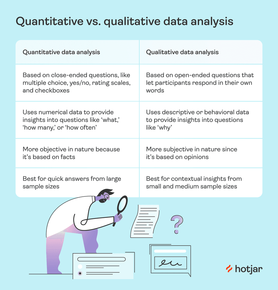
The bottom line: quantitative data analysis and qualitative data analysis are complementary processes. They work hand-in-hand to tell you what’s happening in your business and why.  

💡 Pro tip: easily toggle between quantitative and qualitative data analysis with Hotjar Funnels . 

The Funnels tool helps you visualize quantitative metrics like drop-off and conversion rates in your sales or conversion funnel to understand when and where users leave your website. You can break down your data even further to compare conversion performance by user segment.

Spot a potential issue? A single click takes you to relevant session recordings , where you see user behaviors like mouse movements, scrolls, and clicks. With this qualitative data to provide context, you'll better understand what you need to optimize to streamline the user experience (UX) and increase conversions .

Hotjar Funnels lets you quickly explore the story behind the quantitative data

4 benefits of quantitative data analysis

There’s a reason product, web design, and marketing teams take time to analyze metrics: the process pays off big time. 

Four major benefits of quantitative data analysis include:

1. Make confident decisions 

With quantitative data analysis, you know you’ve got data-driven insights to back up your decisions . For example, if you launch a concept testing survey to gauge user reactions to a new logo design, and 92% of users rate it ‘very good’—you'll feel certain when you give the designer the green light. 

Since you’re relying less on intuition and more on facts, you reduce the risks of making the wrong decision. (You’ll also find it way easier to get buy-in from team members and stakeholders for your next proposed project. 🙌)

2. Reduce costs

By crunching the numbers, you can spot opportunities to reduce spend . For example, if an ad campaign has lower-than-average click-through rates , you might decide to cut your losses and invest your budget elsewhere. 

Or, by analyzing ecommerce metrics , like website traffic by source, you may find you’re getting very little return on investment from a certain social media channel—and scale back spending in that area.

3. Personalize the user experience

Quantitative data analysis helps you map the customer journey , so you get a better sense of customers’ demographics, what page elements they interact with on your site, and where they drop off or convert . 

These insights let you better personalize your website, product, or communication, so you can segment ads, emails, and website content for specific user personas or target groups.

4. Improve user satisfaction and delight

Quantitative data analysis lets you see where your website or product is doing well—and where it falls short for your users . For example, you might see stellar results from KPIs like time on page, but conversion rates for that page are low. 

These quantitative insights encourage you to dive deeper into qualitative data to see why that’s happening—looking for moments of confusion or frustration on session recordings, for example—so you can make adjustments and optimize your conversions by improving customer satisfaction and delight.

💡Pro tip: use Net Promoter Score® (NPS) surveys to capture quantifiable customer satisfaction data that’s easy for you to analyze and interpret. 

With an NPS tool like Hotjar, you can create an on-page survey to ask users how likely they are to recommend you to others on a scale from 0 to 10. (And for added context, you can ask follow-up questions about why customers selected the rating they did—rich qualitative data is always a bonus!)

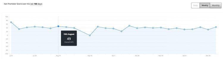
Hotjar graphs your quantitative NPS data to show changes over time

4 steps to effective quantitative data analysis 

Quantitative data analysis sounds way more intimidating than it actually is. Here’s how to make sense of your company’s numbers in just four steps:

1. Collect data

Before you can actually start the analysis process, you need data to analyze. This involves conducting quantitative research and collecting numerical data from various sources, including: 

Interviews or focus groups 

Website analytics

Observations, from tools like heatmaps or session recordings

Questionnaires, like surveys or on-page feedback widgets

Just ensure the questions you ask in your surveys are close-ended questions—providing respondents with select choices to choose from instead of open-ended questions that allow for free responses.

Hotjar’s pricing plans survey template provides close-ended questions

 2. Clean data

Once you’ve collected your data, it’s time to clean it up. Look through your results to find errors, duplicates, and omissions. Keep an eye out for outliers, too. Outliers are data points that differ significantly from the rest of the set—and they can skew your results if you don’t remove them.

By taking the time to clean your data set, you ensure your data is accurate, consistent, and relevant before it’s time to analyze. 

3. Analyze and interpret data

At this point, your data’s all cleaned up and ready for the main event. This step involves crunching the numbers to find patterns and trends via mathematical and statistical methods. 

Two main branches of quantitative data analysis exist: 

Descriptive analysis : methods to summarize or describe attributes of your data set. For example, you may calculate key stats like distribution and frequency, or mean, median, and mode.

Inferential analysis : methods that let you draw conclusions from statistics—like analyzing the relationship between variables or making predictions. These methods include t-tests, cross-tabulation, and factor analysis. (For more detailed explanations and how-tos, head to our guide on quantitative data analysis methods.)

Then, interpret your data to determine the best course of action. What does the data suggest you do ? For example, if your analysis shows a strong correlation between email open rate and time sent, you may explore optimal send times for each user segment.

4. Visualize and share data

Once you’ve analyzed and interpreted your data, create easy-to-read, engaging data visualizations—like charts, graphs, and tables—to present your results to team members and stakeholders. Data visualizations highlight similarities and differences between data sets and show the relationships between variables.

Software can do this part for you. For example, the Hotjar Dashboard shows all of your key metrics in one place—and automatically creates bar graphs to show how your top pages’ performance compares. And with just one click, you can navigate to the Trends tool to analyze product metrics for different segments on a single chart. 

Hotjar Trends lets you compare metrics across segments

Discover rich user insights with quantitative data analysis

Conducting quantitative data analysis takes a little bit of time and know-how, but it’s much more manageable than you might think. 

By choosing the right methods and following clear steps, you gain insights into product performance and customer experience —and you’ll be well on your way to making better decisions and creating more customer satisfaction and loyalty.

FAQs about quantitative data analysis

What is quantitative data analysis.

Quantitative data analysis is the process of making sense of numerical data through mathematical calculations and statistical tests. It helps you identify patterns, relationships, and trends to make better decisions.

How is quantitative data analysis different from qualitative data analysis?

Quantitative and qualitative data analysis are both essential processes for making sense of quantitative and qualitative research .

Quantitative data analysis helps you summarize and interpret numerical results from close-ended questions to understand what is happening. Qualitative data analysis helps you summarize and interpret non-numerical results, like opinions or behavior, to understand why the numbers look like they do.

 If you want to make strong data-driven decisions, you need both.

What are some benefits of quantitative data analysis?

Quantitative data analysis turns numbers into rich insights. Some benefits of this process include: 

Making more confident decisions

Identifying ways to cut costs

Personalizing the user experience

Improving customer satisfaction

What methods can I use to analyze quantitative data?

Quantitative data analysis has two branches: descriptive statistics and inferential statistics. 

Descriptive statistics provide a snapshot of the data’s features by calculating measures like mean, median, and mode. 

Inferential statistics , as the name implies, involves making inferences about what the data means. Dozens of methods exist for this branch of quantitative data analysis, but three commonly used techniques are: 

Cross tabulation

Factor analysis

• Search Search Please fill out this field.
• Understanding QA
• Quantitative vs. Qualitative Analysis

Example of Quantitative Analysis in Finance

Drawbacks and limitations of quantitative analaysis, using quantitative finance outside of finance, the bottom line.

• Quantitative Analysis

Quantitative Analysis (QA): What It Is and How It's Used in Finance

Ariel Courage is an experienced editor, researcher, and former fact-checker. She has performed editing and fact-checking work for several leading finance publications, including The Motley Fool and Passport to Wall Street.

Investopedia / Hilary Allison

Quantitative analysis (QA) refers to methods used to understand the behavior of financial markets and make more informed investment or trading decisions. It involves the use of mathematical and statistical techniques to analyze financial data. For instance, by examining past stock prices, earnings reports, and other information, quantitative analysts, often called “ quants ,” aim to forecast where the market is headed.

Unlike fundamental analysis that might focus on a company's management team or industry conditions, quantitative analysis relies chiefly on crunching numbers and complex computations to derive actionable insights.

Quantitative analysis can be a powerful tool, especially in modern markets where data is abundant and computational tools are advanced, enabling a more precise examination of the financial landscape. However, many also believe that the raw numbers produced by quantitative analysis should be combined with the more in-depth understanding and nuance afforded by qualitative analysis .

Key Takeaways

• Quantitative analysis (QA) is a set of techniques that use mathematical and statistical modeling, measurement, and research to understand behavior.
• Quantitative analysis presents financial information in terms of a numerical value.
• It's used for the evaluation of financial instruments and for predicting real-world events such as changes in GDP.
• While powerful, quantitative analysis has some drawbacks that can be supplemented with qualitative analysis.

Understanding Quantitative Analysis

Quantitative analysis (QA) in finance refers to the use of mathematical and statistical techniques to analyze financial & economic data and make trading, investing, and risk management decisions.

QA starts with data collection, where quants gather a vast amount of financial data that might affect the market. This data can include anything from stock prices and company earnings to economic indicators like inflation or unemployment rates. They then use various mathematical models and statistical techniques to analyze this data, looking for trends, patterns, and potential investment opportunities. The outcome of this analysis can help investors decide where to allocate their resources to maximize returns or minimize risks.

Some key aspects of quantitative analysis in finance include:

• Statistical analysis - this aspect of quantitative analysis involves examining data to identify trends and relationships, build predictive models, and make forecasts. Techniques used can include regression analysis , which helps in understanding relationships between variables; time series analysis , which looks at data points collected or recorded at a specific time; and Monte Carlo simulations , a mathematical technique that allows you to account for uncertainty in your analyses and forecasts. Through statistical analysis, quants can uncover insights that may not be immediately apparent, helping investors and financial analysts make more informed decisions.
• Algorithmic trading - this entails using computer algorithms to automate the trading process. Algorithms can be programmed to carry out trades based on a variety of factors such as timing, price movements, liquidity changes, and other market signals. High-frequency trading (HFT), a type of algorithmic trading, involves making a large number of trades within fractions of a second to capitalize on small price movements. This automated approach to trading can lead to more efficient and often profitable trading strategies.
• Risk modeling - risk is an inherent part of financial markets. Risk modeling involves creating mathematical models to measure and quantify various risk exposures within a portfolio. Methods used in risk modeling include Value-at-Risk (VaR) models, scenario analysis , and stress testing . These tools help in understanding the potential downside and uncertainties associated with different investment scenarios, aiding in better risk management and mitigation strategies.
• Derivatives pricing - derivatives are financial contracts whose value is derived from other underlying assets like stocks or bonds. Derivatives pricing involves creating mathematical models to evaluate these contracts and determine their fair prices and risk profiles. A well-known model used in this domain is the Black-Scholes model , which helps in pricing options contracts . Accurate derivatives pricing is crucial for investors and traders to make sound financial decisions regarding buying, selling, or hedging with derivatives.
• Portfolio optimization - This is about constructing a portfolio in such a way that it yields the highest possible expected return for a given level of risk. Techniques like Modern Portfolio Theory (MPT) are employed to find the optimal allocation of assets within a portfolio. By analyzing various asset classes and their expected returns, risks, and correlations, quants can suggest the best mix of investments to achieve specific financial goals while minimizing risk.

The overall goal is to use data, math, statistics, and software to make more informed financial decisions, automate processes, and ultimately generate greater risk-adjusted returns.

Quantitative analysis is widely used in central banking, algorithmic trading, hedge fund management, and investment banking activities. Quantitative analysts, employ advanced skills in programming, statistics, calculus, linear algebra etc. to execute quantitative analysis.

Quantitative Analysis vs. Qualitative Analysis

Quantitative analysis relies heavily on numerical data and mathematical models to make decisions regarding investments and financial strategies. It focuses on the measurable, objective data that can be gathered about a company or a financial instrument.

But analysts also evaluate information that is not easily quantifiable or reduced to numeric values to get a better picture of a company's performance. This important qualitative data can include reputation, regulatory insights, or employee morale. Qualitative analysis thus focuses more on understanding the underlying qualities of a company or a financial instrument, which may not be immediately quantifiable.

Quantitative isn't the opposite of qualitative analysis. They're different and often complementary philosophies. They each provide useful information for informed decisions. When used together. better decisions can be made than using either one in isolation.

Some common uses of qualitative analysis include:

• Management Evaluation: Qualitative analysis is often better at evaluating a company's management team, their experience, and their ability to lead the company toward growth. While quantifiable metrics are useful, they often cannot capture the full picture of management's ability and potential. For example, the leadership skills, vision, and corporate culture instilled by management are intangible factors that can significantly impact a company's success, yet are difficult to measure with numbers alone.
• Industry Analysis: It also includes an analysis of the industry in which the company operates, the competition, and market conditions. For instance, it can explore how changes in technology or societal behaviors could impact the industry. Qualitative approaches can also better identify barriers to entry or exit, which can affect the level of competition and profitability within the industry.
• Brand Value and Company Reputation: The reputation of a company, its brand value, and customer loyalty are also significant factors considered in qualitative analysis. Understanding how consumers perceive the brand, their level of trust, and satisfaction can provide insights into customer loyalty and the potential for sustained revenue. This can be done through focus groups, surveys, or interviews.
• Regulatory Environment: The regulatory environment, potential legal issues, and other external factors that could impact a company are also analyzed qualitatively. Evaluating a company's compliance with relevant laws, regulations, and industry standards to ascertain its legal standing and the potential risk of legal issues. In addition, understanding a company's ethical practices and social responsibility initiatives, that can influence its relationship with stakeholders and the community at large.

Suppose you are interested in investing in a particular company, XYZ Inc. One way to evaluate its potential as an investment is by analyzing its past financial performance using quantitative analysis. Let's say, over the past five years, XYZ Inc. has been growing its revenue at an average rate of 8% per year. You decide to use regression analysis to forecast its future revenue growth. Regression analysis is a statistical method used to examine the relationship between variables.

After collecting the necessary data, you run a simple linear regression with the year as the independent variable and the revenue as the dependent variable. The output gives you a regression equation, let's say, R e v e n u e = 100 + 8 ( Y e a r ) Revenue=100+8(Year) R e v e n u e = 100 + 8 ( Y e a r ) . This equation suggests that for every year, the revenue of XYZ Inc. increases by $8 million, starting from a base of $100 million. This quantitative insight could be instrumental in helping you decide whether XYZ Inc. represents a good investment opportunity based on its historical revenue growth trend.

However, while you can quantify revenue growth for the firm and make predictions, the reasons for why may not be apparent from quantitative number crunching.

Augmenting with Qualitative Analysis

Qualitative analysis can provide a more nuanced understanding of XYZ Inc.'s potential. You decide to delve into the company's management and industry reputation. Through interviews, reviews, and industry reports, you find that the management team at XYZ Inc. is highly regarded with a track record of successful ventures. Moreover, the company has a strong brand value and a loyal customer base.

Additionally, you assess the industry in which XYZ Inc. operates and find it to be stable with a steady demand for the products that XYZ Inc. offers. The regulatory environment is also favorable, and the company has a good relationship with the local communities in which it operates.

By analyzing these qualitative factors, you obtain a more comprehensive understanding of the company's operational environment, the competence of its management team, and its reputation in the market. This qualitative insight complements the quantitative analysis, providing you with a well-rounded view of XYZ Inc.'s investment potential.

Combining both quantitative and qualitative analyses could therefore lead to a more informed investment decision regarding XYZ Inc.

Quantitative analysis, while powerful, comes with certain limitations:

• Data Dependency: Quantitative analysis is heavily dependent on the quality and availability of numerical data. If the data is inaccurate, outdated, or incomplete, the analysis and the subsequent conclusions drawn will be flawed. As they say, 'garbage-in, garbage-out'.
• Complexity: The methods and models used in quantitative analysis can be very complex, requiring a high level of expertise to develop, interpret, and act upon. This complexity can also make it difficult to communicate findings to individuals who lack a quantitative background.
• Lack of Subjectivity: Quantitative analysis often overlooks qualitative factors like management quality, brand reputation, and other subjective factors that can significantly affect a company's performance or a financial instrument's value. In other words, you may have the 'what' without the 'why' or 'how.' Qualitative analysis can augment this blind spot.
• Assumption-based Modeling: Many quantitative models are built on assumptions that may not hold true in real-world situations. For example, assumptions about normal distribution of returns or constant volatility may not reflect actual market conditions.
• Over-reliance on Historical Data: Quantitative analysis often relies heavily on historical data to make predictions about the future. However, past performance is not always indicative of future results, especially in rapidly changing markets or unforeseen situations like economic crises.
• Inability to Capture Human Emotion and Behavior: Markets are often influenced by human emotions and behaviors which can be erratic and hard to predict. Quantitative analysis, being number-driven, struggles to properly account for these human factors.
• Cost and Time Intensive: Developing accurate and reliable quantitative models can be time-consuming and expensive. It requires skilled personnel, sophisticated software tools, and often, extensive computational resources.
• Overfitting: There's a risk of overfitting , where a model might perform exceedingly well on past data but fails to predict future outcomes accurately because it's too tailored to past events.
• Lack of Flexibility: Quantitative models may lack the flexibility to adapt to new information or changing market conditions quickly, which can lead to outdated or incorrect analysis.
• Model Risk: There's inherent model risk involved where the model itself may have flaws or errors that can lead to incorrect analysis and potentially significant financial losses.

Understanding these drawbacks is crucial for analysts and decision-makers to interpret quantitative analysis results accurately and to balance them with qualitative insights for more holistic decision-making.

Quantitative analysis is a versatile tool that extends beyond the realm of finance into a variety of fields. In the domain of social sciences, for instance, it's used to analyze behavioral patterns, social trends, and the impact of policies on different demographics. Researchers employ statistical models to examine large datasets, enabling them to identify correlations, causations, and trends that can provide a deeper understanding of human behaviors and societal dynamics. Similarly, in the field of public policy, quantitative analysis plays a crucial role in evaluating the effectiveness of different policies, analyzing economic indicators, and forecasting the potential impacts of policy changes. By providing a method to measure and analyze data, it aids policymakers in making informed decisions based on empirical evidence.

In the arena of healthcare, quantitative analysis is employed for clinical trials, genetic research, and epidemiological studies to name a few areas. It assists in analyzing patient data, evaluating treatment outcomes, and understanding disease spread and its determinants. Meanwhile, in engineering and manufacturing, it's used to optimize processes, improve quality control, and enhance operational efficiency. By analyzing data related to production processes, material properties, and operational performance, engineers can identify bottlenecks, optimize workflows, and ensure the reliability and quality of products. Additionally, in the field of marketing, quantitative analysis is fundamental for market segmentation, advertising effectiveness, and consumer satisfaction studies. It helps marketers understand consumer preferences, the impact of advertising campaigns, and the market potential for new products. Through these diverse applications, quantitative analysis serves as a bedrock for data-driven decision-making, enabling professionals across different fields to derive actionable insights from complex data.

What Is Quantitative Analysis Used for in Finance?

Quantitative analysis is used by governments, investors, and businesses (in areas such as finance, project management, production planning, and marketing) to study a certain situation or event, measure it, predict outcomes, and thus help in decision-making. In finance, it's widely used for assessing investment opportunities and risks. For instance, before venturing into investments, analysts rely on quantitative analysis to understand the performance metrics of different financial instruments such as stocks, bonds, and derivatives. By delving into historical data and employing mathematical and statistical models, they can forecast potential future performance and evaluate the underlying risks. This practice isn't just confined to individual assets; it's also essential for portfolio management. By examining the relationships between different assets and assessing their risk and return profiles, investors can construct portfolios that are optimized for the highest possible returns for a given level of risk.

What Kind of Education Do You Need to Be a Quant?

Individuals pursuing a career in quantitative analysis usually have a strong educational background in quantitative fields like mathematics, statistics, computer science, finance, economics, or engineering. Advanced degrees (Master’s or Ph.D.) in quantitative disciplines are often preferred, and additional coursework or certifications in finance and programming can also be beneficial.

What Is the Difference Between Quantitative Analysis and Fundamental Analysis?

While both rely on the use of math and numbers, fundamental analysis takes a broader approach by examining the intrinsic value of a security. It dives into a company's financial statements, industry position, the competence of the management team, and the economic environment in which it operates. By evaluating factors like earnings, dividends, and the financial health of a company, fundamental analysts aim to ascertain the true value of a security and whether it is undervalued or overvalued in the market. This form of analysis is more holistic and requires a deep understanding of the company and the industry in which it operates.

How Does Artificial Intelligence (AI) Influence Quantitative Analysis?

Quantitative analysis often intersects with machine learning (ML) and other forms of artificial intelligence (AI). ML and AI can be employed to develop predictive models and algorithms based on the quantitative data. These technologies can automate the analysis process, handle large datasets, and uncover complex patterns or trends that might be difficult to detect through traditional quantitative methods.

Quantitative analysis is a mathematical approach that collects and evaluates measurable and verifiable data in order to evaluate performance, make better decisions, and predict trends. Unlike qualitative analysis, quantitative analysis uses numerical data to provide an explanation of "what" happened, but not "why" those events occurred.

DeFusco, R. A., McLeavey, D. W., Pinto, J. E., Runkle, D. E., & Anson, M. J. (2015). Quantitative investment analysis . John Wiley & Sons.

University of Sydney. " On Becoming a Quant ," Page 1

Linsmeier, Thomas J., and Neil D. Pearson. " Value at risk ." Financial analysts journal 56, no. 2 (2000): 47-67.

Fischer, Black, and Myron Scholes, " The Pricing of Options and Corporate Liabilities ." Journal of Political Economy, vol. 81, no. 3, 1974, pp. 637-654.

Francis, J. C., & Kim, D. (2013). Modern portfolio theory: Foundations, analysis, and new developments . John Wiley & Sons.

Kaczynski, D., Salmona, M., & Smith, T. (2014). " Qualitative research in finance ." Australian Journal of Management , 39 (1), 127-135.

• Terms of Service
• Editorial Policy
• Privacy Policy
• Your Privacy Choices

• USC Libraries
• Research Guides

Organizing Your Social Sciences Research Paper

• Quantitative Methods
• Purpose of Guide
• Design Flaws to Avoid
• Independent and Dependent Variables
• Glossary of Research Terms
• Reading Research Effectively
• Narrowing a Topic Idea
• Broadening a Topic Idea
• Extending the Timeliness of a Topic Idea
• Academic Writing Style
• Applying Critical Thinking
• Choosing a Title
• Making an Outline
• Paragraph Development
• Research Process Video Series
• Executive Summary
• The C.A.R.S. Model
• Background Information
• The Research Problem/Question
• Theoretical Framework
• Citation Tracking
• Content Alert Services
• Evaluating Sources
• Primary Sources
• Secondary Sources
• Tiertiary Sources
• Scholarly vs. Popular Publications
• Qualitative Methods
• Insiderness
• Using Non-Textual Elements
• Limitations of the Study
• Common Grammar Mistakes
• Writing Concisely
• Avoiding Plagiarism
• Footnotes or Endnotes?
• Further Readings
• Generative AI and Writing
• USC Libraries Tutorials and Other Guides
• Bibliography

Quantitative methods emphasize objective measurements and the statistical, mathematical, or numerical analysis of data collected through polls, questionnaires, and surveys, or by manipulating pre-existing statistical data using computational techniques . Quantitative research focuses on gathering numerical data and generalizing it across groups of people or to explain a particular phenomenon.

Babbie, Earl R. The Practice of Social Research . 12th ed. Belmont, CA: Wadsworth Cengage, 2010; Muijs, Daniel. Doing Quantitative Research in Education with SPSS . 2nd edition. London: SAGE Publications, 2010.

Need Help Locating Statistics?

Resources for locating data and statistics can be found here:

Statistics & Data Research Guide

Characteristics of Quantitative Research

Your goal in conducting quantitative research study is to determine the relationship between one thing [an independent variable] and another [a dependent or outcome variable] within a population. Quantitative research designs are either descriptive [subjects usually measured once] or experimental [subjects measured before and after a treatment]. A descriptive study establishes only associations between variables; an experimental study establishes causality.

Quantitative research deals in numbers, logic, and an objective stance. Quantitative research focuses on numeric and unchanging data and detailed, convergent reasoning rather than divergent reasoning [i.e., the generation of a variety of ideas about a research problem in a spontaneous, free-flowing manner].

Its main characteristics are :

• The data is usually gathered using structured research instruments.
• The results are based on larger sample sizes that are representative of the population.
• The research study can usually be replicated or repeated, given its high reliability.
• Researcher has a clearly defined research question to which objective answers are sought.
• All aspects of the study are carefully designed before data is collected.
• Data are in the form of numbers and statistics, often arranged in tables, charts, figures, or other non-textual forms.
• Project can be used to generalize concepts more widely, predict future results, or investigate causal relationships.
• Researcher uses tools, such as questionnaires or computer software, to collect numerical data.

The overarching aim of a quantitative research study is to classify features, count them, and construct statistical models in an attempt to explain what is observed.

  Things to keep in mind when reporting the results of a study using quantitative methods :

• Explain the data collected and their statistical treatment as well as all relevant results in relation to the research problem you are investigating. Interpretation of results is not appropriate in this section.
• Report unanticipated events that occurred during your data collection. Explain how the actual analysis differs from the planned analysis. Explain your handling of missing data and why any missing data does not undermine the validity of your analysis.
• Explain the techniques you used to "clean" your data set.
• Choose a minimally sufficient statistical procedure ; provide a rationale for its use and a reference for it. Specify any computer programs used.
• Describe the assumptions for each procedure and the steps you took to ensure that they were not violated.
• When using inferential statistics , provide the descriptive statistics, confidence intervals, and sample sizes for each variable as well as the value of the test statistic, its direction, the degrees of freedom, and the significance level [report the actual p value].
• Avoid inferring causality , particularly in nonrandomized designs or without further experimentation.
• Use tables to provide exact values ; use figures to convey global effects. Keep figures small in size; include graphic representations of confidence intervals whenever possible.
• Always tell the reader what to look for in tables and figures .

NOTE:   When using pre-existing statistical data gathered and made available by anyone other than yourself [e.g., government agency], you still must report on the methods that were used to gather the data and describe any missing data that exists and, if there is any, provide a clear explanation why the missing data does not undermine the validity of your final analysis.

Babbie, Earl R. The Practice of Social Research . 12th ed. Belmont, CA: Wadsworth Cengage, 2010; Brians, Craig Leonard et al. Empirical Political Analysis: Quantitative and Qualitative Research Methods . 8th ed. Boston, MA: Longman, 2011; McNabb, David E. Research Methods in Public Administration and Nonprofit Management: Quantitative and Qualitative Approaches . 2nd ed. Armonk, NY: M.E. Sharpe, 2008; Quantitative Research Methods. Writing@CSU. Colorado State University; Singh, Kultar. Quantitative Social Research Methods . Los Angeles, CA: Sage, 2007.

Basic Research Design for Quantitative Studies

Before designing a quantitative research study, you must decide whether it will be descriptive or experimental because this will dictate how you gather, analyze, and interpret the results. A descriptive study is governed by the following rules: subjects are generally measured once; the intention is to only establish associations between variables; and, the study may include a sample population of hundreds or thousands of subjects to ensure that a valid estimate of a generalized relationship between variables has been obtained. An experimental design includes subjects measured before and after a particular treatment, the sample population may be very small and purposefully chosen, and it is intended to establish causality between variables. Introduction The introduction to a quantitative study is usually written in the present tense and from the third person point of view. It covers the following information:

• Identifies the research problem -- as with any academic study, you must state clearly and concisely the research problem being investigated.
• Reviews the literature -- review scholarship on the topic, synthesizing key themes and, if necessary, noting studies that have used similar methods of inquiry and analysis. Note where key gaps exist and how your study helps to fill these gaps or clarifies existing knowledge.
• Describes the theoretical framework -- provide an outline of the theory or hypothesis underpinning your study. If necessary, define unfamiliar or complex terms, concepts, or ideas and provide the appropriate background information to place the research problem in proper context [e.g., historical, cultural, economic, etc.].

Methodology The methods section of a quantitative study should describe how each objective of your study will be achieved. Be sure to provide enough detail to enable the reader can make an informed assessment of the methods being used to obtain results associated with the research problem. The methods section should be presented in the past tense.

• Study population and sampling -- where did the data come from; how robust is it; note where gaps exist or what was excluded. Note the procedures used for their selection;
• Data collection – describe the tools and methods used to collect information and identify the variables being measured; describe the methods used to obtain the data; and, note if the data was pre-existing [i.e., government data] or you gathered it yourself. If you gathered it yourself, describe what type of instrument you used and why. Note that no data set is perfect--describe any limitations in methods of gathering data.
• Data analysis -- describe the procedures for processing and analyzing the data. If appropriate, describe the specific instruments of analysis used to study each research objective, including mathematical techniques and the type of computer software used to manipulate the data.

Results The finding of your study should be written objectively and in a succinct and precise format. In quantitative studies, it is common to use graphs, tables, charts, and other non-textual elements to help the reader understand the data. Make sure that non-textual elements do not stand in isolation from the text but are being used to supplement the overall description of the results and to help clarify key points being made. Further information about how to effectively present data using charts and graphs can be found here .

• Statistical analysis -- how did you analyze the data? What were the key findings from the data? The findings should be present in a logical, sequential order. Describe but do not interpret these trends or negative results; save that for the discussion section. The results should be presented in the past tense.

Discussion Discussions should be analytic, logical, and comprehensive. The discussion should meld together your findings in relation to those identified in the literature review, and placed within the context of the theoretical framework underpinning the study. The discussion should be presented in the present tense.

• Interpretation of results -- reiterate the research problem being investigated and compare and contrast the findings with the research questions underlying the study. Did they affirm predicted outcomes or did the data refute it?
• Description of trends, comparison of groups, or relationships among variables -- describe any trends that emerged from your analysis and explain all unanticipated and statistical insignificant findings.
• Discussion of implications – what is the meaning of your results? Highlight key findings based on the overall results and note findings that you believe are important. How have the results helped fill gaps in understanding the research problem?
• Limitations -- describe any limitations or unavoidable bias in your study and, if necessary, note why these limitations did not inhibit effective interpretation of the results.

Conclusion End your study by to summarizing the topic and provide a final comment and assessment of the study.

• Summary of findings – synthesize the answers to your research questions. Do not report any statistical data here; just provide a narrative summary of the key findings and describe what was learned that you did not know before conducting the study.
• Recommendations – if appropriate to the aim of the assignment, tie key findings with policy recommendations or actions to be taken in practice.
• Future research – note the need for future research linked to your study’s limitations or to any remaining gaps in the literature that were not addressed in your study.

Black, Thomas R. Doing Quantitative Research in the Social Sciences: An Integrated Approach to Research Design, Measurement and Statistics . London: Sage, 1999; Gay,L. R. and Peter Airasain. Educational Research: Competencies for Analysis and Applications . 7th edition. Upper Saddle River, NJ: Merril Prentice Hall, 2003; Hector, Anestine. An Overview of Quantitative Research in Composition and TESOL . Department of English, Indiana University of Pennsylvania; Hopkins, Will G. “Quantitative Research Design.” Sportscience 4, 1 (2000); "A Strategy for Writing Up Research Results. The Structure, Format, Content, and Style of a Journal-Style Scientific Paper." Department of Biology. Bates College; Nenty, H. Johnson. "Writing a Quantitative Research Thesis." International Journal of Educational Science 1 (2009): 19-32; Ouyang, Ronghua (John). Basic Inquiry of Quantitative Research . Kennesaw State University.

Strengths of Using Quantitative Methods

Quantitative researchers try to recognize and isolate specific variables contained within the study framework, seek correlation, relationships and causality, and attempt to control the environment in which the data is collected to avoid the risk of variables, other than the one being studied, accounting for the relationships identified.

Among the specific strengths of using quantitative methods to study social science research problems:

• Allows for a broader study, involving a greater number of subjects, and enhancing the generalization of the results;
• Allows for greater objectivity and accuracy of results. Generally, quantitative methods are designed to provide summaries of data that support generalizations about the phenomenon under study. In order to accomplish this, quantitative research usually involves few variables and many cases, and employs prescribed procedures to ensure validity and reliability;
• Applying well established standards means that the research can be replicated, and then analyzed and compared with similar studies;
• You can summarize vast sources of information and make comparisons across categories and over time; and,
• Personal bias can be avoided by keeping a 'distance' from participating subjects and using accepted computational techniques .

Babbie, Earl R. The Practice of Social Research . 12th ed. Belmont, CA: Wadsworth Cengage, 2010; Brians, Craig Leonard et al. Empirical Political Analysis: Quantitative and Qualitative Research Methods . 8th ed. Boston, MA: Longman, 2011; McNabb, David E. Research Methods in Public Administration and Nonprofit Management: Quantitative and Qualitative Approaches . 2nd ed. Armonk, NY: M.E. Sharpe, 2008; Singh, Kultar. Quantitative Social Research Methods . Los Angeles, CA: Sage, 2007.

Limitations of Using Quantitative Methods

Quantitative methods presume to have an objective approach to studying research problems, where data is controlled and measured, to address the accumulation of facts, and to determine the causes of behavior. As a consequence, the results of quantitative research may be statistically significant but are often humanly insignificant.

Some specific limitations associated with using quantitative methods to study research problems in the social sciences include:

• Quantitative data is more efficient and able to test hypotheses, but may miss contextual detail;
• Uses a static and rigid approach and so employs an inflexible process of discovery;
• The development of standard questions by researchers can lead to "structural bias" and false representation, where the data actually reflects the view of the researcher instead of the participating subject;
• Results provide less detail on behavior, attitudes, and motivation;
• Researcher may collect a much narrower and sometimes superficial dataset;
• Results are limited as they provide numerical descriptions rather than detailed narrative and generally provide less elaborate accounts of human perception;
• The research is often carried out in an unnatural, artificial environment so that a level of control can be applied to the exercise. This level of control might not normally be in place in the real world thus yielding "laboratory results" as opposed to "real world results"; and,
• Preset answers will not necessarily reflect how people really feel about a subject and, in some cases, might just be the closest match to the preconceived hypothesis.

Research Tip

Finding Examples of How to Apply Different Types of Research Methods

SAGE publications is a major publisher of studies about how to design and conduct research in the social and behavioral sciences. Their SAGE Research Methods Online and Cases database includes contents from books, articles, encyclopedias, handbooks, and videos covering social science research design and methods including the complete Little Green Book Series of Quantitative Applications in the Social Sciences and the Little Blue Book Series of Qualitative Research techniques. The database also includes case studies outlining the research methods used in real research projects. This is an excellent source for finding definitions of key terms and descriptions of research design and practice, techniques of data gathering, analysis, and reporting, and information about theories of research [e.g., grounded theory]. The database covers both qualitative and quantitative research methods as well as mixed methods approaches to conducting research.

SAGE Research Methods Online and Cases

• << Previous: Qualitative Methods
• Next: Insiderness >>
• Last Updated: Apr 20, 2024 2:57 PM
• URL: https://libguides.usc.edu/writingguide

Thank you for visiting nature.com. You are using a browser version with limited support for CSS. To obtain the best experience, we recommend you use a more up to date browser (or turn off compatibility mode in Internet Explorer). In the meantime, to ensure continued support, we are displaying the site without styles and JavaScript.

• View all journals
• Explore content
• About the journal
• Publish with us
• Sign up for alerts
• Published: 11 April 2024

Quantitative text analysis

• Kristoffer L. Nielbo   ORCID: orcid.org/0000-0002-5116-5070 1 ,
• Folgert Karsdorp 2 ,
• Melvin Wevers   ORCID: orcid.org/0000-0001-8177-4582 3 ,
• Alie Lassche   ORCID: orcid.org/0000-0002-7607-0174 4 ,
• Rebekah B. Baglini   ORCID: orcid.org/0000-0002-2836-5867 5 ,
• Mike Kestemont 6 &
• Nina Tahmasebi   ORCID: orcid.org/0000-0003-1688-1845 7  

Nature Reviews Methods Primers volume  4 , Article number:  25 ( 2024 ) Cite this article

3175 Accesses

53 Altmetric

Metrics details

• Computational science
• Interdisciplinary studies

Text analysis has undergone substantial evolution since its inception, moving from manual qualitative assessments to sophisticated quantitative and computational methods. Beginning in the late twentieth century, a surge in the utilization of computational techniques reshaped the landscape of text analysis, catalysed by advances in computational power and database technologies. Researchers in various fields, from history to medicine, are now using quantitative methodologies, particularly machine learning, to extract insights from massive textual data sets. This transformation can be described in three discernible methodological stages: feature-based models, representation learning models and generative models. Although sequential, these stages are complementary, each addressing analytical challenges in the text analysis. The progression from feature-based models that require manual feature engineering to contemporary generative models, such as GPT-4 and Llama2, signifies a change in the workflow, scale and computational infrastructure of the quantitative text analysis. This Primer presents a detailed introduction of some of these developments, offering insights into the methods, principles and applications pertinent to researchers embarking on the quantitative text analysis, especially within the field of machine learning.

You have full access to this article via your institution.

Similar content being viewed by others

Augmenting interpretable models with large language models during training

Chandan Singh, Armin Askari, … Jianfeng Gao

An open source machine learning framework for efficient and transparent systematic reviews

Rens van de Schoot, Jonathan de Bruin, … Daniel L. Oberski

The shaky foundations of large language models and foundation models for electronic health records

Michael Wornow, Yizhe Xu, … Nigam H. Shah

Introduction

Qualitative analysis of textual data has a long research history. However, a fundamental shift occurred in the late twentieth century when researchers began investigating the potential of computational methods for text analysis and interpretation 1 . Today, researchers in diverse fields, such as history, medicine and chemistry, commonly use the quantification of large textual data sets to uncover patterns and trends, producing insights and knowledge that can aid in decision-making and offer novel ways of viewing historical events and current realities. Quantitative text analysis (QTA) encompasses a range of computational methods that convert textual data or natural language into structured formats before subjecting them to statistical, mathematical and numerical analysis. With the increasing availability of digital text from numerous sources, such as books, scientific articles, social media posts and online forums, these methods are becoming increasingly valuable, facilitated by advances in computational technology.

Given the widespread application of QTA across disciplines, it is essential to understand the evolution of the field. As a relatively consolidated field, QTA embodies numerous methods for extracting and structuring information in textual data. It gained momentum in the late 1990s as a subset of the broader domain of data mining, catalysed by advances in database technologies, software accessibility and computational capabilities 2 , 3 . However, it is essential to recognize that the evolution of QTA extends beyond computer science and statistics. It has heavily incorporated techniques and algorithms derived from  corpus linguistics 4 , computer linguistics 5 and information retrieval 6 . Today, QTA is largely driven by  machine learning , a crucial component of  data science , artificial intelligence (AI) and natural language processing (NLP).

Methods of QTA are often referred to as techniques that are innately linked with specific tasks (Table  1 ). For example, the sentiment analysis aims to determine the emotional tone of a text 7 , whereas entity and concept extraction seek to identify and categorize elements in a text, such as names, locations or key themes 8 , 9 . Text classification refers to the task of sorting texts into groups with predefined labels 10 — for example, sorting news articles into semantic categories such as politics, sports or entertainment. In contrast to machine-learning tasks that use supervised learning , text clustering, which uses  unsupervised learning , involves finding naturally occurring groups in unlabelled texts 11 . A significant subset of tasks primarily aim to simplify and structure natural language. For example, representation learning includes tasks that automatically convert texts into numerical representations, which can then be used for other tasks 12 . The lines separating these techniques can be blurred and often vary depending on the research context. For example, topic modelling, a type of statistical modelling used for concept extraction, serves simultaneously as a clustering and representation learning technique 13 , 14 , 15 .

QTA, similar to machine learning, learns from observation of existing data rather than by manipulating variables as in scientific experiments 16 . In QTA, experiments encompass the design and implementation of empirical tests to explore and evaluate the performance of models, algorithms and techniques in relation to specific tasks and applications. In practice, this involves a series of steps. First, text data are collected from real-world sources such as newspaper articles, patient records or social media posts. Then, a specific type of machine-learning model is selected and designed. The model could be a tree-based decision model, a clustering technique or more complex encoder–decoder models for tasks such as translation. Subsequently, the selected model is trained on the collected data, learning to make categorizations or predictions based on the data. The performance of the model is evaluated using predominantly intrinsic performance metrics (such as accuracy for a classification task) and, to a lesser degree, extrinsic metrics that measure how the output of the model impacts a broader task or system.

Three distinct methodological stages can be observed in the evolution of QTA: feature-based models, representation learning models and generative models (Fig.  1 ). Feature-based models use efficient machine-learning techniques, collectively referred to as shallow learning, which are ideal for tabular data but require manual feature engineering. They include models based on  bag-of-words models , decision trees and support vector machines and were some of the first methods applied in QTA. Representation learning models use deep learning techniques that automatically learn useful features from text. These models include architectures such as the highly influential  transformer architecture 17 and techniques such as masked language modelling, as used in language representation models such as Bidirectional Encoder Representations from Transformers (BERT) 18 . BERT makes use of the transformer architecture, as do most other large language models after the introduction of the architecture 17 . This shift towards automatic learning representations marked an important advance in natural language understanding. Generative models, trained using autoregressive techniques, represent the latest frontier. These models, such as generative pre-trained transformer GPT-3 (ref. 19 ), GPT-4 and Llama2 (ref. 20 ), can generate coherent and contextually appropriate responses and are powerful tools for natural language generation. Feature-based models preceded representation learning, which in turn preceded generative models.

a , Feature-based models in which data undergo preprocessing to generate features for model training and prediction. b , Representation learning models that can be trained from scratch using raw data or leverage pre-trained models fine-tuned with specific data. c , Generative models in which a prompt guides the generative deep learning model, potentially augmented by external data, to produce a result.

Although these models are temporally ordered, they do not replace each other. Instead, each offers unique methodological features and is suitable for different tasks. The progress from small models with limited computing capacity to today’s large models with billions of parameters encapsulates the transformation in the scale and complexity of the QTA.

The evolution of these models reflects the advancement of machine-learning infrastructure, particularly in the emergence and development of tooling frameworks. These frameworks, exemplified by platforms such as scikit-learn 21 and Hugging Face 22 , have served as essential infrastructure for democratizing and simplifying the implementation of increasingly sophisticated models. They offer user-friendly interfaces that mask the complexities of the algorithms, thereby empowering researchers to harness advanced methodologies with minimal prerequisite knowledge and coding expertise. The advent of high-level generative models such as GPT-3 (ref. 19 ), GPT-4 and Llama2 (ref. 20 ) marks milestones in the progression. Renowned for their unprecedented language understanding and generation capabilities, these models have the potential to redefine access to the sophisticated text analysis by operating on natural language prompts, effectively bypassing the traditional need for coding. It is important to emphasize that these stages represent an abstraction that points to fundamental changes to the workflow and underlying infrastructure of QTA.

This Primer offers an accessible introduction to QTA methods, principles and applications within feature-based models, representation learning and generative models. The focus is on how to extract and structure textual data using machine learning to enable quantitative analysis. The Primer is particularly suitable for researchers new to the field with a pragmatic interest in these techniques. By focusing on machine-learning methodologies, a comprehensive overview of several key workflows currently in use is presented. The focus consciously excludes traditional count-based and rule-based methods, such as keyword and collocation analysis. This decision is guided by the current dominance of machine learning in QTA, in terms of both performance and scalability. However, it is worth noting that machine-learning methods can encompass traditional approaches where relevant, adding to their versatility and broad applicability. The experiments in QTA are presented, including problem formulation, data collection, model selection and evaluation techniques. The results and real-world applications of these methodologies are discussed, underscoring the importance of reproducibility and robust data management practices. The inherent limitations and potential optimizations within the field are addressed, charting the evolution from basic feature-based approaches to advanced generative models. The article concludes with a forward-looking discussion on the ethical implications, practical considerations and methodological advances shaping the future of QTA. Regarding tools and software, references to specific libraries and packages are omitted as they are relatively easy to identify given a specific task. Generally, the use of programming languages that are well suited for QTA is recommended, such as Python, R and Julia, but it is also acknowledged that graphical platforms for data analysis provide similar functionalities and may be better suited for certain disciplines.

Experimentation

In QTA, the term experiment assumes a distinct character. Rather than mirroring the controlled conditions commonly associated with randomized controlled trials, it denotes a structured procedure that aims to validate, refine and compare models and findings. QTA experiments provide a platform for testing ideas, establishing hypotheses and paving the way for advancement. At the heart of these experiments lies a model — a mathematical and computational embodiment of discernible patterns drawn from data. A model can be considered a learned function that captures the intricate relationship between textual features and their intended outcomes, allowing for informed decisions on unseen data. For example, in the sentiment analysis, a model learns the association between specific words or phrases and the emotions they convey, later using this knowledge to assess the sentiment of new texts.

The following section delineates the required steps for a QTA experiment. This step-by-step description encompasses everything from problem definition and data collection to the nuances of model selection, training and validation. It is important to distinguish between two approaches in QTA: training or fine-tuning a model, and applying a (pre-trained) model (Fig.  1 ). In the first approach, a model is trained or fine-tuned to solve a QTA task. In the second approach, a pre-trained model is used to solve a QTA task. Finally, it is important to recognize that experimentation, much like other scientific pursuits, is inherently iterative. This cyclic process ensures that the devised models are not just accurate but also versatile enough to be applicable in real-world scenarios.

Problem formulation

Problem formulation is a crucial first step in QTA, laying the foundation for subsequent analysis and experimentation. This process involves several key considerations, which, when clearly defined beforehand, contributes to the clarity and focus of the experiment. First, every QTA project begins with the identification of a research question. The subsequent step is to determine the scope of the analysis, which involves defining the boundaries of the study, such as the time period, the type of texts to be analysed or the geographical or demographic considerations.

An integral part of this process is to identify the nature of the analytical task. This involves deciding whether the study is a classification task, for example, in which data are categorized into predefined classes; a clustering task, in which data are grouped based on similarities without predefined categories; or another type of analysis. The choice of task has significant implications for both the design of the study and the selection of appropriate data and analytical techniques. For instance, a classification task such as sentiment analysis requires clearly defined categories and suitable labelled data, whereas a clustering task might be used in the exploratory data analysis to uncover underlying patterns in the data.

After selecting data to support the analysis, an important next step is deciding on the level of analysis. QTA can be conducted at various levels, such as the document-level, paragraph-level, sentence-level or even word-level. The choice largely depends on the research question, as well as the nature of the data set.

Classification

A common application of a classification task in QTA is the sentiment analysis. For instance, in analysing social media comments, a binary classification might be employed in which comments are labelled as positive or negative. This straightforward example showcases the formulation of a problem in which the objective is clear-cut classification based on predefined sentiment labels. In this case, the level of analysis might be at the sentence level, focusing on the sentiment expressed in each individual comment.

From this sentence-level information, it is possible to extrapolate to general degrees of sentiment. This is often done when companies want to survey their products or when political parties want to analyse their support, for example, to determine how many people are positive or negative towards the party 23 . Finally, from changing degrees of sentiment, one can extract the most salient aspects that form this sentiment: recurring positive or negative sentiments towards price or quality, or different political issues.

Modelling of themes

The modelling of themes involves the identification of prevalent topics, for example, in a collection of news articles. Unlike the emotion classification task, here the researcher is interested in uncovering underlying themes or topics, rather than classifying texts into predefined categories. This problem formulation requires an approach that can discern and categorize emergent topics from the textual data, possibly at the document level, to capture broader thematic elements. This can be done without using any predefined hypotheses 24 , or by steering topic models towards certain seed topics (such as a given scientific paper or book) 25 . Using such topic detection tools, it can be determined how prevalent topics are in different time periods or across genre to determine significance or impact of both topics and authors.

Modelling of temporal change

Consider a study aiming to track the evolution of literary themes over time. In this scenario, the problem formulation would involve not only the selection of texts and features but also a temporal dimension, in which changes in themes are analysed across different time periods. This type of analysis might involve examining patterns and trends in literary themes, requiring a longitudinal approach to text analysis, for example, in the case of scientific themes or reports about important events 26 or themes as proxy for meaning change 27 . Often, when longitudinal analysis is considered, additional challenges are involved, such as statistical properties relating to increasing or decreasing quantity or quality of data that can influence results, see, for example, refs. 28 , 29 , 30 , 31 .

In similar fashion, temporal analysis of changing data happens in a multitude of disciplines from linguistics, as in computational detection of words that experience change in meaning 32 , to conceptual change in history 33 , poetry 34 , medicine 35 , political science 36 , 37 and to the study of ethnical biases and racism 38 , 39 , 40 .

The GIGO principle, meaning ‘garbage in, garbage out’, is ever present in QTA because without high-quality data even the most sophisticated models can falter, rendering analyses inaccurate or misleading. To ensure robustness in, for example, social media data, its inherently informal and dynamic nature must be acknowledged, often characterized by non-standard grammar, slang and evolving language use. Robustness here refers to the ability of the data to provide reliable, consistent analysis, despite these irregularities. This requires implementing specialized preprocessing techniques that can handle such linguistic variability without losing contextual meaning. For example, rather than discarding non-standard expressions or internet-specific abbreviations, these elements should be carefully processed to preserve their significant role in conveying sentiment and meaning. Additionally, ensuring representativeness and diversity in the data set is crucial; collecting data across different demographics, topics and time frames can mitigate biases and provide a more comprehensive view of the discourse if this is needed. Finally, it is important to pay attention to errors, anomalies and irregularities in the data, such as optical character recognition errors and missing values, and in some cases take steps to remediate these in preprocessing. More generally, it is crucial to emphasize that the quality of a given data set depends on the research question. Grammatically well-formed sentences may be high-quality data for training a linguistic parser; social media could never be studied as people on social media rarely abide by the rules of morphology and syntax. This underscores the vital role of data not just as input but also as an essential component that dictates the success and validity of the analytical endeavour.

Data acquisition

Depending on the research objective, data sets can vary widely in their characteristics. For the emotion classifier, a data set could consist of many social media comments. If the task is to train or fine-tune a model, each comment should be annotated with its corresponding sentiment label (labels). If the researcher wants to apply a pre-trained model, then only a subset of the data must be annotated to test the generalizability of the model. Labels can be annotated manually or automatically, for instance, by user-generated ratings, such as product reviews or social media posts, for example. Training data should have sufficient coverage of the phenomenon under investigation to capture its linguistic characteristics. For the emotion classifier, a mix of comments are needed, ranging from brief quips to lengthy rants, offering diverse emotional perspectives. Adhering to the principle that there are no data like more data, the breadth and depth of such a data set significantly enhance the accuracy of the model. Traditionally, data collection was arduous, but today QTA researchers can collect data from the web and archives using dedicated software libraries or an  application programming interface . For analogue data, optical character recognition and handwritten text recognition offer efficient conversion to machine-readable formats 41 . Similarly, for auditory language data, automatic speech recognition has emerged as an invaluable tool 42 .

Data preprocessing

In feature-based QTA, manual data preprocessing is one of the most crucial and time-consuming stages. Studies suggest that researchers can spend up to 80% of their project time refining and managing their data 43 . A typical preprocessing workflow for feature-based techniques requires data cleaning and text normalization. Standard procedures include transforming all characters to lower case for uniformity, eliminating punctuation marks and removing high-frequency functional words such as ‘and’, ‘the’ or ‘is’. However, it is essential to recognize that these preprocessing strategies should be closely aligned with the specific research question at hand. For example, in the sentiment analysis, retaining emotive terms and expressions is crucial, whereas in syntactic parsing, the focus might be on the structural elements of language, requiring a different approach to what constitutes ‘noise’ in the data. More nuanced challenges arise in ensuring the integrity of a data set. For instance, issues with character encoding require attention to maintain language and platform interoperability, which means resorting to universally accepted encoding formats such as UTF-8. Other normalization steps, such as  stemming or lemmatization , involve reducing words to their root forms to reduce lexical variation. Although these are standard practices, their application might vary depending on the research objective. For example, in a study focusing on linguistic diversity, aggressive stemming may erase important stylistic or dialectal markers. Many open-source software libraries exist nowadays that can help automate such processes for various languages. The impact of these steps on research results underscores the necessity of a structured and well-documented approach to preprocessing, including detailed reporting of all preprocessing steps and software used, to ensure that analyses are both reliable and reproducible. The practice of documenting preprocessing is crucial, yet often overlooked, reinforcing its importance for the integrity of research.

With representation learning and generative techniques, QTA has moved towards end-to-end models that take raw text input such as social media comments and directly produces the final desired output such as emotion classification, handling all intermediate steps without manual intervention 44 . However, removal of non-textual artefacts such as HTML codes and unwanted textual elements such as pornographic material can still require substantial work to prepare data to train an end-to-end model.

Annotation and labelling

Training and validating a (pre-trained) model requires annotating the textual data set. These data sets come in two primary flavours: pre-existing collections with established labels and newly curated sets awaiting annotation. Although pre-existing data sets offer a head-start, owing to their readymade labels, they must be validated to ensure alignment with research objectives. By contrast, crafting a data set from scratch confers flexibility to tailor the data to precise research needs, but it also ushers in the intricate task of collecting and annotating data. Annotation is a meticulous endeavour that demands rigorous consistency and reliability. To ensure inter-annotator agreement (IAA) 45 , for example, annotations from multiple annotators are compared using metrics such as  Fleiss’ kappa ( κ ) to assess consistency. A high IAA score not only indicates annotation consistency but also lends confidence in the reliability of the data set. There is no universally accepted manner to interpret κ statistics, although κ  ≥ 0. 61 is generally considered to indicate ‘substantial agreement’ 46 .

Various tools and platforms support the annotation process. Specialized software for research teams provides controlled environments for annotation tasks. Crowdsourcing is another approach, in which tasks are distributed among a large group of people. This can be done through non-monetized campaigns, focusing on volunteer participation or gamification strategies to encourage user engagement in annotation tasks 47 . Monetized platforms, such as Amazon Mechanical Turk, represent a different facet of crowdsourcing in which microtasks are outsourced for financial compensation. It is important to emphasize that, although these platforms offer a convenient way to gather large-scale annotations, they raise ethical concerns regarding worker exploitation and fair compensation. Critical studies, such as those of Paolacci, Chandler and Ipeirotis 48 and Bergvall-Kåreborn and Howcroft 49 , highlight the need for awareness and responsible use of such platforms in research contexts.

Provenance and ethical considerations

Data provenance is of utmost importance in QTA. Whenever feasible, preference should be given to open and well-documented data sets that comply with the principles of FAIR (findable, accessible, interoperable and reusable) 50 . However, the endeavour to harness data, especially online, requires both legal and ethical considerations. For instance, the General Data Protection Regulation delineates the rights of European data subjects and sets stringent data collection and usage criteria. Unstructured data can complicate standard techniques for data depersonalization (for example, data masking, swapping and pseudonymization). Where these techniques fail, differential privacy may be a viable alternative to ensure that the probability of any specific output of the model does not depend on the information of any individual in the data set 51 .

Recognition of encoded biases is equally important. Data sets can inadvertently perpetuate cultural biases towards attributes such as gender and race, resulting in sampling bias. Such bias compromises research integrity and can lead to models that reinforce existing inequalities. Gender, for instance, can have subtle effects that are not easily detected in textual data 52 . A popular approach to rectifying biases is  data augmentation , which can be used to increase the diversity of a data set without collecting new data 53 . This is achieved by applying transformations to existing textual data, creating new and diverse examples. The main goal of data augmentation is to improve model generalization by exposing it to a broader range of data variations.

Model selection and design

Model selection and design set the boundaries for efficiency, accuracy and generalizability of any QTA experiment. Choosing the right model architecture depends on several considerations and will typically require experimentation to compare the performance of multiple models. Although the methodological trajectory of QTA provides a roadmap, specific requirements of the task, coupled with available data volume, often guide the final choice. Although some tasks require that the model be trained from scratch owing to, for instance, transparency and security requirements, it has become common to use pre-trained models that provide text representations originating from training on massive data sets. Pre-trained models can be fine-tuned for a specific task, for example, emotion classification. Training feature-based models may be optimal for smaller data sets, focusing on straightforward interpretability. By contrast, the complexities of expansive textual data often require representation learning or generative models. In QTA, achieving peak performance is a trade-off among model interpretability, computational efficiency and predictive power. As the sophistication of a model grows, hyperparameter tuning, regularization and loss function require meticulous consideration. These decisions ensure that a model is not only accurate but also customized for research-specific requirements.

Training and evaluation

During the training phase, models learn patterns from the data to predict or classify textual input. Evaluation is the assessment phase that determines how the trained model performs on unseen data. Evaluation serves multiple purposes, but first and foremost, it is used to assess how well the model performs on a specific task using metrics such as accuracy, precision and recall. For example, knowing how accurately the emotion classifier identifies emotions is crucial for any research application. Evaluation of this model also allows researchers to assess whether it is biased towards common emotions and whether it generalizes across different types of text sources. When an emotion classifier is trained on social media posts, a common practice, its effectiveness can be evaluated on different data types, such as patient journals or historical newspapers, to determine its performance across varied contexts. Evaluation enables us to compare multiple models to select the most relevant for the research problem. Additional evaluation involves hyperparameter tuning, resource allocation, benchmarking and model fairness audits.

Overfitting is often a challenge in model training, which can occur when a model is excessively tailored to the peculiarities of the training data and becomes so specialized that its generalizability is compromised. Such a model performs accurately on the specific data set but underperforms on unseen examples. Overfitting can be counteracted by dividing the data into three distinct subsets: the training set, the validation set and the test set. The training set is the primary data set from which the model learns patterns, adjusts its weights and fine-tunes itself based on the labelled examples provided. The validation set is used to monitor and assess the performance of the model during training. It acts as a checkpoint, guides hyperparameter tuning and ensures that the model is not veering off track. The test set is the final held-out set on which the performance of the model is evaluated. The test set is akin to a final examination, assessing how well the model generalizes to unseen data. If a pre-trained model is used, only the data sets used to fine-tune the model are necessary to evaluate the model.

The effectiveness of any trained model is gauged not just by how well it fits the training data but also by its performance on unseen samples. Evaluation metrics provide objective measures to assess performance on validation and test sets as well as unseen examples. The evaluation process is fundamental to QTA experiments, as demonstrated in the text classification research 10 . Several evaluation metrics are used to measure performance. The most prominent are accuracy (the proportion of all predictions that are correct), precision (the proportion of positive predictions that are actually correct) and recall (the proportion of actual positives that were correctly identified). The F1 score amalgamates precision and recall and emerges as a balanced metric, especially when class distributions are skewed. An effective evaluation typically uses various complementary metrics.

In QTA, a before-and-after dynamic often emerges, encapsulating the transformation from raw data to insightful conclusions 54 . This paradigm is especially important in QTA, in which the raw textual data can be used to distil concrete answers to research questions. In the preceding section, the preliminary before phase, the process of setting up an experiment in QTA, is explored with emphasis on the importance of model training and thorough evaluation to ensure robustness. For the after phase, the focus pivots to the critical step of applying the trained model to new, unseen data, aiming to answer the research questions that guide exploration.

Research questions in QTA are often sophisticated and complex, encompassing a range of inquiries either directly related to the text being analysed or to the external phenomena the text reflects. The link between the output of QTA models and the research question is often vague and under-specified. When dealing with a complex research question, for example, the processes that govern the changing attitudes towards different migrant groups, the outcome of any one QTA model is often insufficient. Even several models might not provide a complete answer to the research question. Consequently, challenges surface during the transition from before to after, from setting up and training to applying and validating. One primary obstacle is the validation difficulty posed by the uniqueness and unseen nature of the new data.

Validating QTA models on new, unseen data introduces a layer of complexity that highlights the need for robust validation strategies, to ensure stability, generalizability and replicability of results. Although the effectiveness of a model might have been calibrated in a controlled setup, its performance can oscillate when exposed to the multifaceted layers of new real-world data. Ensuring consistent model performance is crucial to deriving meaningful conclusions aligned with the research question. This dual approach of applying the model and subsequently evaluating its performance in fresh terrains is central to the after phase of QTA. In addition to validating the models, the results that stem from the models need to be validated with respect to the research question. The results need to be representative for the data as a whole; they need to be stable such that the answer does not change if different choices are made in the before phase; and they need to provide an answer to the research question at hand.

This section provides a road map for navigating the application of QTA models to new data and a chart of methodologies for evaluating the outcomes in line with the research question (questions). The goal is to help researchers cross the bridge between the theoretical foundations of QTA and its practical implementation, illuminating the steps that support the successful application and assessment of QTA models. The ensuing discussion covers validation strategies that cater to the challenges brought forth by new data, paving the way towards more insightful analysis.

Application to new data

After the training and evaluation phases have been completed, the next step is applying the trained model to new, unseen data (Fig.  2 ). The goal is to ensure that the application aligns with the research questions and aids in extracting meaningful insights. However, applying the model to new data is not without challenges.

Although the illustration demonstrates a feature-based modelling approach, the fundamental principle remains consistent across different methodologies, be it feature-based, representation learning or generative. A critical consideration is ensuring the consistency in content and preprocessing between the training data and any new data subjected to inference.

Before application of the model, it is crucial to preprocess the new data similar to the training data. This involves routine tasks such as tokenization and lemmatization, but also demands vigilance for anomalies such as divergent text encoding formats or missing values. In such cases, additional preprocessing steps might be required and should be documented carefully to ensure reproducibility.

Another potential hurdle is the discrepancy in data distributions between the training data and new data, often referred to as domain shift. If not addressed, domain shifts may hinder the efficacy of the model. Even thematically, new data may unearth categories or motifs that were absent during training, thus challenging the interpretative effectiveness of the model. In such scenarios, transfer learning or domain adaptation techniques are invaluable tools for adjusting the model so that it aligns better with the characteristics of the new data. In transfer learning, a pre-trained model provides general language understanding and is fine-tuned with a small data set for a specific task (for example, fine-tuning a large language model such as GPT or BERT for emotion classification) 55 , 56 . Domain adaptation techniques similarly adjust a model from a source domain to a target domain; for example, an emotion classifier trained on customer reviews can be adapted to rate social media comments.

Given the iterative nature of QTA, applying a model is not necessarily an end point; it may simply be a precursor to additional refinement and analysis. Therefore, the adaptability of the validation strategies is paramount. As nuances in the new data are uncovered, validation strategies may need refinement or re-adaptation to ensure the predictions of the model remain accurate and insightful, ensuring that the answers to the research questions are precise and meaningful. Through careful application and handling of the new data, coupled with adaptable validation strategies, researchers can significantly enhance the value of their analysis in answering the research question.

Evaluation metrics

QTA models are often initially developed and validated on well-defined data sets, ensuring their reliability in controlled settings. This controlled environment allows researchers to set aside a held-out test set to gauge the performance of a model, simulating how it will fare on new data. The real world, however, is considerably more complex than any single data set can capture. The challenge is how to transition from a controlled setting to novel data sets.

One primary challenge is the mismatch between the test set and real-world texts. Even with the most comprehensive test sets, capturing the linguistic variation, topic nuance and contextual subtlety present in new data sets is not a trivial task, and researchers should not be overconfident regarding the universal applicability of a model 57 . The situation does not become less complicated when relying on pre-trained or off-the-shelf models. The original training data and its characteristics might not be transparent or known with such models. Without appropriate documentation, predicting the behaviour of a model on new data may become a speculative endeavour 58 .

The following sections summarize strategies for evaluating models on new data.

Model confidence scores

In QTA, models often generate confidence or probability scores alongside predictions, indicating the confidence of the model in its accuracy. However, high scores do not guarantee correctness and can be misleading. Calibrating the model refines these scores to align better with true label likelihoods 59 . This is especially crucial in high-stakes QTA applications such as legal or financial text analysis 60 . Calibration techniques adjust the original probability estimates, enhancing model reliability and the trustworthiness of predictions, thereby addressing potential discrepancies between the expressed confidence of the model and its actual performance.

Precision at k

Precision at k (P@ k ) is useful for tasks with rankable predictions, such as determining document relevance. P@ k measures the proportion of relevant items among the top- k ranked items, providing a tractable way to gauge the performance of a model on unseen data by focusing on a manageable subset, especially when manual evaluation of the entire data set is infeasible. Although primarily used in information retrieval and recommender system , its principles apply to QTA, in which assessing the effectiveness of a model in retrieving or categorizing relevant texts is crucial.

External feedback mechanisms

Soliciting feedback from domain experts is invaluable in evaluating models on unseen data. Domain experts can provide qualitative insights into the output of the model, identifying strengths and potential missteps. For example, in topic modelling, domain experts can assess the coherence and relevance of the generated topics. This iterative feedback helps refine the model, ensuring its robustness and relevance when applied to new, unseen data, thereby bridging the gap between model development and practical application.

Software and tools

When analysing and evaluating QTA models on unseen data, researchers often turn to specialized tools designed to increase model transparency and explain model predictions. Among these tools, LIME (Local Interpretable Model-agnostic Explanations) 61 and SHAP (SHapley Additive exPlanations) 62 have gained traction for their ability to provide insights into model behaviour per instance, which is crucial when transitioning to new data domains.

LIME focuses on the predictions of machine-learning models by creating locally faithful explanations. It operates by perturbing the input data and observing how the predictions change, making it a useful tool to understand model behaviour on unseen data. Using LIME, researchers can approximate complex models with simpler, interpretable models locally around the prediction point. By doing so, they can gain insight into how different input features contribute to the prediction of the model, which can be instrumental in understanding how a model might generalize to new, unseen data.

SHAP, by contrast, provides a unified measure of feature importance across different data types, including text. It uses game theoretic principles to attribute the output of machine-learning models to their input features. This method allows for a more precise understanding of how different words or phrases in text data influence the output of the model, thereby offering a clearer picture of the behaviour of the model on new data domains. The SHAP library provides examples of how to explain predictions from text analysis models applied to various NLP tasks including sentiment analysis, text generation and translation.

Both LIME and SHAP offer visual tools to help researchers interpret the predictions of the model, making it easier to identify potential issues when transitioning to unseen data domains. For instance, visualizations allow researchers to identify words or phrases that heavily influence the decisions of the model, which can be invaluable in understanding and adjusting the model for new text data.

Interpretation

Interpretability is paramount in QTA as it facilitates the translation of complex model outcomes into actionable insights relevant to the research questions. The nature and complexity of the research question can significantly mould the interpretation process by requiring various information signals to be extracted from the text, see, for example, ref.  63 . For example, in predicting election outcomes based on sentiments expressed in social media 64 , it is essential to account for both endorsements of parties as expressed in the text and a count of individuals (that is, statistical signals) to avoid the results being skewed because some individuals make a high number of posts. It is also important to note whether voters of some political parties are under-represented in the data.

The complexity amplifies when delving into understanding why people vote (or do not vote) for particular parties and what arguments sway their decisions. Such research questions demand a more comprehensive analysis, often necessitating the amalgamation of insights from multiple models, for example, argument mining, aspect-based sentiment analysis and topic models. There is a discernible gap between the numerical or categorical outputs of QTA models — such as classification values, proportions of different stances or vectors representing individual words — and the nuanced understanding required to fully address the research question. This understanding is achieved either using qualitative human analysis or applying additional QTA methods and extracts a diverse set of important arguments in support of different stances, or provides qualitative summaries of a large set of different comments. Because it is not only a matter of ‘what’ results are found using QTA, but the value that can be attributed to those results.

When interpreting the results of a computational model applied to textual data for a specific research question, it is important to consider the completeness of the answer (assess whether the output of the model sufficiently addresses the research question or whether there are aspects left unexplored), the necessity of additional models (determine whether the insights from more models are needed to fully answer the research question), the independence or co-dependence of results (in cases in which multiple models are used, ascertain whether their results are independent or co-dependent and adjust for any overlap in insights accordingly), clarify how the results are used to support an answer (such as the required occurrence of a phenomenon in the text to accept a concept, or how well a derived topic is understood and represented) and the effect of methodology (evaluate the impact of the chosen method or preprocessing on the results, ensuring the reproducibility and robustness of the findings against changes in preprocessing or methods).

Using these considerations alongside techniques such as LIME and SHAP enhances the evaluation of the application of the model. For instance, in a scenario in which a QTA model is used to analyse customer reviews, LIME and SHAP could provide nuanced insights on a peer-review basis and across all reviews, respectively. Such insights are pivotal in assessing the alignment of the model with the domain-relevant information necessary to address the research questions and in making any adjustments needed to enhance its relevance and performance. Moreover, these techniques and considerations catalyse a dialogue between model and domain experts, enabling a more nuanced evaluation that extends beyond mere quantitative metrics towards a qualitative understanding of the application of the model.

Applications

The applicability of QTA can be found in its ability to address research questions across various disciplines. Although these questions are varied and tasks exist that do not fit naturally into categories, they can be grouped into four primary tasks: extracting, categorizing, predicting and generating. Each task is important in advancing understanding of large textual data sets, either by examining phenomena specific to a text or by using texts as a proxy for phenomena outside the text.

Extracting information

In the context of QTA, information extraction goes beyond mere data retrieval; it also involves identifying and assessing patterns, structures and entities within extensive textual data sets. At its core are techniques such as frequency analysis, in which words or sets of words are counted and their occurrences plotted over periods to reveal trends or shifts in usage and syntactical analysis, which targets specific structures such as nouns, verbs and intricate patterns such as passive voice constructions. Named entity recognition pinpoints entities such as persons, organizations and locations using syntactic information and lexicons of entities.

These methodologies have proven useful in various academic domains. For example, humanities scholars have applied QTA to track the evolution of literary themes 65 . Word embedding has been used to shed light on broader sociocultural shifts such as the conceptual change of ‘racism’, or detecting moments of linguistic change in American foreign relations 40 , 66 . In a historical context, researchers have used diachronic word embeddings to scrutinize the role of abolitionist newspapers in influencing public opinion about the abolition of slavery, revealing pathways of lexical semantic influence, distinguishing leaders from followers and identifying others who stood out based on the semantic changes that swept through this period 67 . Topic modelling and topic linkage (the extent to which two topics tend to co-appear) have been applied to user comments and submissions from the ‘subreddit’ group r/TheRedPill to study how people interact with ideology 68 . In the medical domain 69 , QTA tools have been used to study narrative structures in personal birth stories. The authors utilized a topic model based on latent Dirichlet allocation (LDA) to not only represent the sequence of events in every story but also detect outlier stories using the probability of transitioning between topics.

Historically, the focus was predominantly on feature-based models that relied on manual feature engineering. Such methods were transparent but rigid, constraining the richness of the textual data. Put differently, given the labour-intensive selection of features and the need to keep them interpretable, the complexity of a text was reduced to a limited set of features. However, the advent of representation learning has catalysed a significant paradigm shift. It enables more nuanced extraction, considers contextual variations and allows for sophisticated trend analysis. Studies using these advanced techniques have been successful in, for example, analysing how gender stereotypes and attitudes towards ethnic minorities in the USA evolved during the twentieth and twenty-first centuries 38 and tracking the emergence of ideas in the domains of politics, law and business through contextual embeddings combined with statistical modelling 70 (Box  1 ).

Box 1 Using text mining to model prescient ideas

Vicinanza et al. 70 focused on the predictive power of linguistic markers within the domains of politics, law and business, positing that certain shifts in language can serve as early indicators of deeper cognitive changes. They identified two primary attributes of prescient ideas: their capacity to challenge existing contextual assumptions, and their ability to foreshadow the future evolution of a domain. To quantify this, they utilized Bidirectional Encoder Representations from Transformers, a type 2 language model, to calculate a metric termed contextual novelty to gauge the predictability of an utterance within the prevailing discourse.

Their study presents compelling evidence that prescient ideas are more likely to emerge from the periphery of a domain than from its core. This suggests that prescience is not solely an individual trait but also significantly influenced by contextual factors. Thus, the researchers extended the notion of prescience to include the environments in which innovative ideas are nurtured, adding another layer to our understanding of how novel concepts evolve and gain acceptance.

Categorizing content

It remains an indispensable task in QTA to categorize content, especially when dealing with large data sets. The challenge is not only logistical but also methodological, demanding sophisticated techniques to ensure precision and utility. Text classification algorithms, supervised or unsupervised, continue to have a central role in labelling and organizing content. They serve crucial functions beyond academic settings; for instance, digital libraries use these algorithms to manage and make accessible their expansive article collections. These classification systems also contribute significantly to the systematic review of the literature, enabling more focused and effective investigations of, for example, medical systematic reviews 71 . In addition, unsupervised techniques such as topic modelling have proven invaluable in uncovering latent subject matter within data sets 72 (Box  2 ). This utility extends to multiple scenarios, from reducing redundancies in large document sets to facilitating the analysis of open-ended survey responses 73 , 74 .

Earlier approaches to categorization relied heavily on feature-based models that used manually crafted features for organization. This traditional paradigm has been disrupted by advances in representation learning, deep neural networks and word embeddings, which has introduced a new age of dynamic unsupervised and semi-supervised techniques for content categorization. GPT models represent another leap forward in text classification tasks, outpacing existing benchmarks across various applications. From the sentiment analysis to text labelling and psychological construct detection, generative models have demonstrated a superior capability for context understanding, including the ability to parse complex linguistic cues such as sarcasm and mixed emotions 75 , 76 , 77 . Although the validity of these models is a matter of debate, they offer explanations for their reasoning, which adds a layer of interpretability.

Box 2 Exploring molecular data with topic modelling

Schneider et al. 72 introduced a novel application of topic modelling to the field of medicinal chemistry. The authors adopt a probabilistic topic modelling approach to organize large molecular data sets into chemical topics, enabling the investigation of relationships between these topics. They demonstrate the effectiveness of the quantitative text analysis method in identifying and retrieving chemical series from molecular sets. The authors are able to reproduce concepts assigned by humans in the identification and retrieval of chemical series from sets of molecules. Using topic modelling, the authors are able to show chemical topics intuitively with data visualization and efficiently extend the method to a large data set (ChEMBL22) containing 1.6 million molecules.

Predicting outcomes

QTA is not limited to understanding or classifying text but extends its reach into predictive analytics, which is an invaluable tool across many disciplines and industries. In the financial realm, sentiment analysis tools are applied to news articles and social media data to anticipate stock market fluctuations 78 . Similarly, political analysts use sentiment analysis techniques to make election forecasts, using diverse data sources ranging from Twitter (now X) feeds to party manifestos 79 . Authorship attribution offers another intriguing facet, in which predictive abilities of the QTA are harnessed to identify potential authors of anonymous or pseudonymous works 80 . A notable instance was the unmasking of J.K. Rowling as the author behind the pseudonym Robert Galbraith 81 . Health care has also tapped into predictive strengths of the QTA: machine-learning models that integrate natural language and binary features from patient records have been shown to have potential as early warning systems to prevent unnecessary mechanical restraint of psychiatric inpatients 82 (Box  3 ).

In the era of feature-based models, predictions often hinged on linear or tree-based structures using manually engineered features. Representation learning introduced embeddings and sequential models that improved prediction capabilities. These learned representations enrich predictive tasks, enhancing accuracy and reliability while decreasing interpretability.

Box 3 Predicting mechanical restraint: assessing the contribution of textual data

Danielsen et al. 82 set out to assess the potential of electronic health text data to predict incidents of mechanical restraint of psychiatric patients. Mechanical restraint is used during inpatient treatments to avert potential self-harm or harm to others. The research team used feature-based supervised machine learning to train a predictive model on clinical notes and health records from the Central Denmark Region, specifically focusing on the first hour of admission data. Of 5,050 patients and 8,869 admissions, 100 patients were subjected to mechanical restraint between 1 h and 3 days after admission. Impressively, a random forest algorithm could predict mechanical restraint with considerable precision, showing an area under the curve of 0.87. Nine of the ten most influential predictors stemmed directly from clinical notes, that is, unstructured textual data. The results show the potential of textual data for the creation of an early detection system that could pave the way for interventions that minimize the use of mechanical restraint. It is important to emphasize that the model was limited by a narrow scope of data from the Central Denmark Region, and by the fact that only initial mechanical restraint episodes were considered (in other words, recurrent incidents were not included in the study).

Generating content

Although the initial QTA methodologies were not centred on content generation, the rise of generative models has been transformative. Models such as GPT-4 and Llama2 (ref. 20 ) have brought forth previously unimagined capabilities, expanding the potential of QTA to create content, including coherent and contextually accurate paragraphs to complete articles. Writers and content creators are now using tools based on models such as GPT-4 to augment their writing processes by offering suggestions or even drafting entire sections of texts. In education, such models aid in developing customized content for students, ensuring adaptive learning 83 . The capacity to create synthetic data also heralds new possibilities. Consider the domain of historical research, in which generative models can simulate textual content, offering speculative yet data-driven accounts of alternate histories or events that might have been; for example, relying on generative models to create computational software agents that simulate human behaviour 84 . However, the risks associated with text-generating models are exemplified by a study in which GPT-3 was used for storytelling. The generated stories were found to exhibit many known gender stereotypes, even when prompts did not contain explicit gender cues or stereotype-related content 85 .

Reproducibility and data deposition

Given the rapidly evolving nature of the models, methods and practices in QTA, reproducibility is essential for validating the results and creating a foundation upon which other researchers can build. Sharing code and trained models in well-documented repositories are important to enable reproducible experiments. However, sharing and depositing raw data can be challenging, owing to the inherent limitations of unstructured data and regulations related to proprietary and sensitive data.

Code and model sharing

In QTA research, using open source code has become the norm and the need to share models and code to foster innovation and collaboration has been widely accepted. QTA is interdisciplinary by nature, and by making code and models public, the field has avoided unnecessary silos and enabled collaboration between otherwise disparate disciplines. A further benefit of open source software is the flexibility and transparency that comes from freely accessing and modifying software to meet specific research needs. Accessibility enables an iterative feedback loop, as researchers can validate, critique and build on the existing work. Software libraries, such as scikit-learn, that have been drivers for adopting machine learning in QTA are testimony to the importance of open source software 21 .

Sharing models is not without challenges. QTA is evolving rapidly, and models may use specific versions of software and hardware configurations that no longer work or that yield different results with other versions or configurations. This variability can complicate the accessibility and reproducibility of research results. The breakthroughs of generative AI in particular have introduced new proprietary challenges to model sharing as data owners and sources raise objections to the use of models that have been trained on their data. This challenge is complicated, but fundamentally it mirrors the disputes about intellectual property rights and proprietary code in software engineering. Although QTA as a field benefits from open source software, individual research institutions may have commercial interests or intellectual property rights related to their software.

On the software side, there is currently a preference for scripting languages, especially Python, that enable rapid development, provide access to a wide selection of software libraries and have a large user community. QTA is converging towards code and model sharing through open source platforms such as GitHub and GitLab with an appropriate open source software license such as the MIT license . Models often come with additional disclaimers or use-based restrictions to promote responsible use of AI, such as in the RAIL licenses . Pre-trained models are also regularly shared on dedicated machine-learning platforms such as Hugging Face 22 to enable efficient fine-tuning and deployment. It is important to emphasize that although these platforms support open science, these services are provided by companies with commercial interests. Open science platforms such as Zenodo and OSF can also be used to share code and models for the purpose of reproducibility.

Popular containerization software has been widely adopted in the machine-learning community and has spread to QTA. Containerization, that is, packaging all parts of a QTA application — including code and other dependencies — into a single standalone unit ensures that model and code run consistently across various computing environments. It offers a powerful solution to challenges such as reproducibility, specifically variability in software and hardware configurations.

Data management and storage

Advances in QTA in recent years are mainly because of the availability of vast amounts of text data and the rise of deep learning techniques. However, the dependency on large unstructured data sets, many of which are proprietary or sensitive, poses unique data management challenges. Pre-trained models irrespective of their use (for example, representation learning or generative) require extensive training on large data sets. When these data sets are proprietary or sensitive, they cannot be readily available, which limits the ability of researchers to reproduce results and develop competitive models. Furthermore, models trained on proprietary data sets often lack transparency regarding their collection and curation processes, which can hide potential biases in the data. Finally, there can be data privacy issues related to training or using models that are trained on sensitive data. Individuals whose data are included may not have given their explicit consent for their information to be used in research, which can pose ethical and legal challenges.

It is a widely adopted practice in QTA to share data and metadata with an appropriate license whenever possible. Data can be deposited in open science platforms such as Zenodo, but specialized machine-learning platforms are also used for this purpose. However, it should be noted that QTA data are rarely unique, unlike experimental data collected through random controlled trials. In many cases, access to appropriate metadata and documentation would enable the data to be reconstructed. In almost all cases, it is therefore strongly recommended that researchers share metadata and documentation for data, as well as code and models, using a standardized document or framework, a so-called datasheet. Although QTA is not committed to one set of principles for (meta)data management, European research institutions are increasingly adopting the FAIR principles 50 .

Documentation

Although good documentation is vital in all fields of software development and research, the reliance of QTA on code, models and large data sets makes documentation particularly crucial for reproducibility. Popular resources for structuring projects include project templating tools and documentation generators such as Cookiecutter and Sphinx . Models are often documented with model cards that provide a detailed overview of the development, capabilities and biases of the model to promote transparency and accountability 86 . Similarly, datasheets or data cards can be used to promote transparency for data used in QTA 87 . Finally, it is considered good practice to provide logs for models that document parameters, metrics and events for QTA experiments, especially during training and fine-tuning. Although not strictly required, logs are also important for documenting the iterative process of model refinement. There are several platforms that support the creation and visualization of training logs ( Weights & Biases and MLflow ).

Limitations and optimizations

The application of QTA requires scrutiny of its inherent limitations and potentials. This section discusses these aspects and elucidates the challenges and opportunities for further refinement.

Limitations in QTA

Defining research questions.

In QTA, the framing of research questions is often determined by the capabilities and limitations of the available text analysis tools, rather than by intellectual inquiry or scientific curiosity. This leads to task-driven limitations, in which inquiry is confined to areas where the tools are most effective. For example, relying solely on bag-of-words models might skew research towards easily quantifiable aspects, distorting the intellectual landscape. Operationalizing broad and nuanced research questions into specific tasks may strip them of their depth, forcing them to conform to the constraints of existing analytical models 88 .

Challenges in interpretation

The representation of language of underlying phenomena is often ambiguous or indirect, requiring careful interpretation. Misinterpretations can arise, leading to challenges related to historical, social and cultural context of a text, in which nuanced meanings that change across time, class and cultures are misunderstood 89 . Overlooking other modalities such as visual or auditory information can lead to a partial understanding of the subject matter and limit the full scope of insights. This can to some extent be remedied by the use of grounded models (such as GPT-4), but it remains a challenge for the community to solve long term.

Determining reliability and validation

The reliability and stability of the conclusions drawn from the QTA require rigorous validation, which is often neglected in practice. Multiple models, possibly on different types of data, should be compared to ensure that conclusions are not artefacts of a particular method or of a different use of the method. Furthermore, cultural phenomena should be evolved to avoid misguided insights. Building a robust framework that allows testing and comparison enhances the integrity and applicability of QTA in various contexts 90 .

Connecting analysis to cultural insights

Connecting text analysis to larger cultural claims necessitates foundational theoretical frameworks, including recognizing linguistic patterns, sociolinguistic variables and theories of cultural evolution that may explain changes. Translating textual patterns into meaningful cultural observations requires understanding how much (or how little) culture is expressed in text so that findings can be generalized beyond isolated observations. A theoretical foundation is vital to translate textual patterns into culturally relevant insights, making QTA a more effective tool for broader cultural analysis.

Balancing factors in machine learning

Balancing factors is critical in aligning machine-learning techniques with research objectives. This includes the trade-off between quality and control. Quality refers to rigorous, robust and valid findings, and control refers to the ability to manage specific variables for clear insights. It is also vital to ensure a balance between quantity and quality in data source to lead to more reliable conclusions. Balance is also needed between correctness and accuracy, in which the former ensures consistent application of rules, and the latter captures the true nature of the text.

From features-based to generative models

QTA has undergone a profound evolution, transitioning from feature-based approaches to representation learning and finally to generative models. This progression demonstrates growing complexity in our understanding of language, reflecting the maturity in the field of QTA. Each stage has its characteristics, strengths and limitations.

In the early stages, feature-based models were both promising and limiting. The simplicity of their design, relying on explicit feature engineering, allowed for the targeted analysis. However, this simplicity limited their ability to grasp complex, high-level patterns in language. For example, the use of bag-of-words models in the sentiment analysis showcased direct applicability, but also revealed limitations in understanding contextual nuances. The task-driven limitations of these models sometimes overshadowed genuine intellectual inquiry. Using a fixed (often modern) list of words with corresponding emotional valences may limit our ability to fully comprehend the complexity of emotional stances in, for example, historical literature. Despite these drawbacks, the ability to customize features provided researchers with a direct and specific understanding of language phenomena that could be informed by specialized domain knowledge 91 .

With the emergence of representation learning, a shift occurred within the field of QTA. These models offered the ability to capture higher-level abstractions, forging a richer understanding of language. Their scalability to handle large data sets and uncover complex relationships became a significant strength. However, this complexity introduced new challenges, such as a loss of specificity in analysis and difficulties in translating broad research questions into specific tasks. Techniques such as Word2Vec enabled the capture of semantic relationships but made it difficult to pinpoint specific linguistic features. Contextualized models, in turn, allow for more specificity, but are typically pre-trained on huge data sets (not available for scrutiny) and then applied to a research question without any discussion of how well the model fits the data at hand. In addition, these contextualized models inundate with information. Instead of providing one representation for a word (similar to Word2Vec does), they provide one representation for each occurrence of the word. Each of these representations is one order of magnitude larger than vectors typical for Word2Vec (768–1,600 dimensions compared with 50–200) and comes in several varieties, one for each of the layers of the mode, typically 12.

The introduction of generative models represents the latest stage of this evolution, providing even greater complexity and potential. Innovative in their design, generative models provide opportunities to address more complex and open-ended research questions. They fuel the generation of new ideas and offer avenues for novel approaches. However, these models are not without their challenges. Their high complexity can make interpretation and validation demanding, and if not properly managed, biases and ethical dilemmas will emerge. The use of generative models in creating synthetic text must be handled with care to avoid reinforcing stereotypes or generating misleading information. In addition, if the enormous amounts of synthetically generated text are used to further train the models, this will lead to a spiral of decaying quality as eventually a majority of the training data will have been generated by machines (the models often fail to distinguish synthetic text from genuine human-created text) 92 . However, it will also allow researchers to draw insights from a machine that is learning on data it has generated itself.

The evolution from feature-based to representation learning to generative models reflects increasing maturity in the field of QTA. As models become more complex, the need for careful consideration, ethical oversight and methodological innovation intensifies. The challenge now lies in ensuring that these methodologies align with intellectual and scientific goals, rather than being constrained by their inherent limitations. This growing complexity mirrors the increasing demands of this information-driven society, requiring interdisciplinary collaboration and responsible innovation. Generative models require a nuanced understanding of the complex interplay between language, culture, time and society, and a clear recognition of constraints of the QTA. Researchers must align their tools with intellectual goals and embrace active efforts to address the challenges through optimization strategies. The evolution in QTA emphasizes not only technological advances but also the necessity of aligning the ever-changing landscape of computational methodologies with research questions. By focusing on these areas and embracing the accompanying challenges, the field can build robust, reliable conclusions and move towards more nuanced applications of the text analysis. This progress marks a significant step towards an enriched exploration of textual data, widening the scope for understanding multifaceted relationships. The road ahead calls for a further integration of theory and practice. It is essential that evolution of QTA ensures that technological advancement serves both intellectual curiosity and ethical responsibility, resonating with the multifaceted dynamics of language, culture, time and society 93 .

Balancing size and quality

In QTA, the relationship between data quantity and data quality is often misconceived. Although large data sets serve as the basis for training expansive language models, they are not always required when seeking answers to nuanced research questions. The wide-ranging scope of large data sets can offer comprehensive insights into broad trends and general phenomena. However, this often comes at the cost of a detailed understanding of context-specific occurrences. An issue such as  frequency bias exemplifies this drawback. Using diverse sampling strategies, such as stratified sampling to ensure representation across different social groups and bootstrapping methods to correct for selection bias, can offer a more balanced, contextualized viewpoint. Also, relying on methods such as burst or change-point detection can help to pinpoint moments of interest in data sets with a temporal dimension. Triangulating these methods across multiple smaller data sets can enhance reliability and depth of the analysis.

The design of machine-learning models should account for both the frequency and the significance of individual data points. In other words, the models should be capable of learning not just from repetitive occurrences but also from singular, yet critical, events. This enables the machine to understand rare but important phenomena such as revolutions, seminal publications or watershed individual actions, which would typically be overlooked in a conventional data-driven approach. The capacity to learn from such anomalies can enhance the interpretative depth of the model, enabling them to offer more nuanced insights.

Although textual data have been the mainstay for computational analyses, it is not the only type of data that matters, especially when the research questions involve cultural and societal nuances. Diverse data types including images, audio recordings and even physical artefacts should be integrated into the research to provide a more rounded analysis. Additionally, sourcing data from varied geographical and sociocultural contexts can bring multiple perspectives into the frame, thus offering a multifaceted understanding that textual data from English sources alone cannot capture.

Ethical, practical and efficient models

The evolving landscape of machine learning, specifically with respect to model design and utility, reflects a growing emphasis on efficiency and interpretive value. One notable shift is towards smaller, more energy-efficient models. This transition is motivated by both environmental sustainability and economic pragmatism. With computational costs soaring and the environmental toll becoming untenable, the demand for smaller models that maintain or even exceed the quality of larger models is escalating 94 .

Addressing the data sources used to train models is equally critical, particularly when considering models that will serve research or policy purposes. The provenance and context of data dictate its interpretive value, requiring models to be designed with a hierarchical evaluation of data sources. Such an approach could improve the understanding of a model of the importance of each data type given a specific context, thereby improving the quality and reliability of its analysis. Additionally, it is important to acknowledge the potential ethical and legal challenges within this process, including the exploitation of workers during the data collection and model development.

Transparency remains another pressing issue as these models become integral to research processes. Future iterations should feature a declaration of content that enumerates not only the origin of the data but also its sociocultural and temporal context, preprocessing steps, any known biases, along with the analytical limitations of the model. This becomes especially important for generative models, which may produce misleading or even harmful content if the original data sources are not properly disclosed and understood. Important steps have already been taken with the construction of model cards and data sheets 95 .

Finally, an emergent concern is the risk of feedback loops compromising the quality of machine-learning models. If a model is trained on its own output, errors and biases risk being amplified over time. This necessitates constant vigilance as it poses a threat to the long-term reliability and integrity of AI models. The creation of a gold-standard version of the Internet, not polluted by AI-generated data, is also important 96 .

Refining the methodology and ethos

The rapid advances in QTA, particularly the rise of generative models, have opened up a discourse that transcends mere technological prowess. Although earlier feature-based models require domain expertise and extensive human input before they could be used, generative models can already generate convincing output based on relatively short prompts. This shift raises crucial questions about the interplay between machine capability and human expertise. The notion that advanced algorithms might eventually replace researchers is a common misplaced apprehension. These algorithms and models should be conceived as tools to enhance human scholarship by automating mundane tasks, spawning new research questions and even offering novel pathways for data analysis that might be too complex or time-consuming for human cognition.

This paradigm shift towards augmentative technologies introduces a nuanced problem-solving framework that accommodates the complexities intrinsic to studying human culture and behaviour. The approach of problem decomposition, a cornerstone in computer science, also proves invaluable here, converting overarching research queries into discrete, operationalizable components. These elements can then be addressed individually through specialized algorithms or models, whose results can subsequently be synthesized into a comprehensive answer. As we integrate increasingly advanced tuning methods into generative models — such as prompt engineering, retrieval augmented generation and parameter-efficient fine-tuning — it is important to remember that these models are tools, not replacements. They are most effective when employed as part of a broader research toolkit, in which their strengths can complement traditional scholarly methods.

Consequently, model selection becomes pivotal and should be intricately aligned with the nature of the research inquiry. Unsupervised learning algorithms such as clustering are well suited to exploratory research aimed at pattern identification. Conversely, confirmatory questions, which seek to validate theories or test hypotheses, are better addressed through supervised learning models such as regression.

The importance of a well-crafted interpretation stage cannot be overstated. This is where the separate analytical threads are woven into a comprehensive narrative that explains how the individual findings conjoin to form a cohesive answer to the original research query. However, the lack of standardization across methodologies is a persistent challenge. This absence hinders the reliable comparison of research outcomes across various studies. To remedy this, a shift towards establishing guidelines or best practices is advocated. These need not be rigid frameworks but could be adapted to fit specific research contexts, thereby ensuring methodological rigor alongside innovative freedom.

Reflecting on the capabilities and limitations of current generative models in QTA research is crucial. Beyond recognizing their utility, the blind spots — questions they cannot answer and challenges they have yet to overcome — need to be addressed 97 , 98 . There is a growing need to tailor these models to account for nuances such as frequency bias and to include various perspectives, possibly through more diverse data sets or a polyvocal approach.

In summary, a multipronged approach that synergizes transparent and informed data selection, ethical and critical perspectives on model building and selection, and an explicit and reproducible result interpretation offers a robust framework for tackling intricate research questions. By adopting such a nuanced strategy, we make strides not just in technological capability but also in the rigor, validity and credibility of QTA as a research tool.

Miner, G. Practical Text Mining and Statistical Analysis for Non-structured Text Data Applications (Academic Press, 2012).

Fayyad, U., Piatetsky-Shapiro, G. & Smyth, P. From data mining to knowledge discovery in databases. AI Mag. 17 , 37 (1996).

Google Scholar  

Hand, D. J. Data mining: statistics and more? Am. Stat. 52 , 112–116 (1998).

Article   Google Scholar  

McEnery, T. & Wilson, A. Corpus Linguistics: An Introduction (Edinburgh University Press, 2001).

Manning, C. D. & Schütze, H. Foundations of Statistical Natural Language Processing 1st edn (The MIT Press, 1999).

Manning, C., Raghavan, P. & Schütze, H. Introduction to Information Retrieval 1st edn (Cambridge University Press, 2008).

Wankhade, M., Rao, A. C. S. & Kulkarni, C. A survey on sentiment analysis methods, applications, and challenges. Artif. Intell. Rev. 55 , 5731–5780 (2022).

Jehangir, B., Radhakrishnan, S. & Agarwal, R. A survey on named entity recognition — datasets, tools, and methodologies. Nat. Lang. Process. J. 3 , 100017 (2023).

Fu, S. et al. Clinical concept extraction: a methodology review. J. Biomed. Inform. 109 , 103526 (2020).

Sebastiani, F. Machine learning in automated text categorization. ACM Comput. Surv. 34 , 1–47 (2002).

Talley, E. M. et al. Database of NIH grants using machine-learned categories and graphical clustering. Nat. Meth. 8 , 443–444 (2011).

Bommasani, R. et al. On the opportunities and risks of foundation models. Preprint at https://arxiv.org/abs/2108.07258 (2022).

Blei, D. M., Ng, A. Y. & Jordan, M. I. Latent Dirichlet allocation. J. Mach. Learn. Res. 3 , 993–1022 (2003).

Angelov, D. Top2Vec: distributed representations of topics. Preprint at https://arxiv.org/abs/2008.09470 (2020).

Barron, A. T. J., Huang, J., Spang, R. L. & DeDeo, S. Individuals, institutions, and innovation in the debates of the French Revolution. Proc. Natl Acad. Sci. USA 115 , 4607–4612 (2018).

Article   ADS   Google Scholar  

Mitchell, T. M. Machine Learning 1st edn (McGraw-Hill, 1997).

Vaswani, A. et al. Attention is all you need. in Advances in Neural Information Processing Systems (eds Guyon, I. et al.) Vol. 30 (Curran Associates, Inc., 2017).

Devlin, J., Chang, M.-W., Lee, K. & Toutanova, K. BERT: pre-training of deep bidirectional transformers for language understanding. https://arxiv.org/abs/1810.04805 (2018).

Brown, T. et al. Language models are few-shot learners. in Advances in Neural Information Processing Systems Vol. 33 (eds Larochelle, H., Ranzato, M., Hadsell, R., Balcan, M. & Lin, H.) 1877–1901 (Curran Associates, Inc., 2020).

Touvron, H. et al. Llama 2: open foundation and fine-tuned chat models. Preprint at https://arxiv.org/abs/2307.09288 (2023).

Pedregosa, F. et al. Scikit-learn: machine learning in Python. J. Mach. Learn. Res. 12 , 2825–2830 (2011).

MathSciNet   Google Scholar  

Wolf, T. et al. Transformers: state-of-the-art natural language processing. in Proc. 2020 Conference on Empirical Methods in Natural Language Processing: System Demonstrations 38–45 (Association for Computational Linguistics, Online, 2020).

Demartini, G., Siersdorfer, S., Chelaru, S. & Nejdl, W. Analyzing political trends in the blogosphere. in Proceedings of the International AAAI Conference on Web and Social Media vol. 5 466–469 (AAAI, 2011).

Goldstone, A. & Underwood, T. The quiet transformations of literary studies: what thirteen thousand scholars could tell us. New Lit. Hist. 45 , 359–384 (2014).

Tangherlini, T. R. & Leonard, P. Trawling in the sea of the great unread: sub-corpus topic modeling and humanities research. Poetics 41 , 725–749 (2013).

Mei, Q. & Zhai, C. Discovering evolutionary theme patterns from text: an exploration of temporal text mining. in Proceedings of the Eleventh ACM SIGKDD International Conference on Knowledge Discovery and Data Mining 198–207 (Association for Computing Machinery, 2005).

Frermann, L. & Lapata, M. A Bayesian model of diachronic meaning change. Trans. Assoc. Comput. Linguist. 4 , 31–45 (2016).

Koplenig, A. Analyzing Lexical Change in Diachronic Corpora . PhD thesis, Mannheim https://nbn-resolving.org/urn:nbn:de:bsz:mh39-48905 (2016).

Dubossarsky, H., Weinshall, D. & Grossman, E. Outta control: laws of semantic change and inherent biases in word representation models. in Proceedings of the 2017 Conference on Empirical Methods in Natural Language Processing 1136–1145 (Association for Computational Linguistics, 2017).

Dubossarsky, H., Hengchen, S., Tahmasebi, N. & Schlechtweg, D. Time-out: temporal referencing for robust modeling of lexical semantic change. in Proc. 57th Annual Meeting of the Association for Computational Linguistics 457–470 (Association for Computational Linguistics, 2019).

Koplenig, A. Why the quantitative analysis of diachronic corpora that does not consider the temporal aspect of time-series can lead to wrong conclusions. Digit. Scholarsh. Humanit. 32 , 159–168 (2017).

Tahmasebi, N., Borin, L. & Jatowt, A. Survey of computational approaches to lexical semantic change detection. Zenodo https://doi.org/10.5281/zenodo.5040302 (2021).

Bizzoni, Y., Degaetano-Orttlieb, S., Fankhauser, P. & Teich, E. Linguistic variation and change in 250 years of English scientific writing: a data-driven approach. Front. Artif. Intell. 3 , 73 (2020).

Haider, T. & Eger, S. Semantic change and emerging tropes in a large corpus of New High German poetry. in Proc. 1st International Workshop on Computational Approaches to Historical Language Change 216–222 (Association for Computational Linguistics, 2019).

Vylomova, E., Murphy, S. & Haslam, N. Evaluation of semantic change of harm-related concepts in psychology. in Proc. 1st International Workshop on Computational Approaches to Historical Language Change 29–34 (Association for Computational Linguistics, 2019).

Marjanen, J., Pivovarova, L., Zosa, E. & Kurunmäki, J. Clustering ideological terms in historical newspaper data with diachronic word embeddings. in 5th International Workshop on Computational History, HistoInformatics 2019 (CEUR-WS, 2019).

Tripodi, R., Warglien, M., Levis Sullam, S. & Paci, D. Tracing antisemitic language through diachronic embedding projections: France 1789–1914. in Proc. 1st International Workshop on Computational Approaches to Historical Language Change 115–125 (Association for Computational Linguistics, 2019).

Garg, N., Schiebinger, L., Jurafsky, D. & Zou, J. Word embeddings quantify 100 years of gender and ethnic stereotypes. Proc. Natl. Acad. Sci. USA 115 , E3635–E3644 (2018).

Wevers, M. Using word embeddings to examine gender bias in Dutch newspapers, 1950–1990. in Proc. 1st International Workshop on Computational Approaches to Historical Language Change 92–97 (Association for Computational Linguistics, 2019).

Sommerauer, P. & Fokkens, A. Conceptual change and distributional semantic models: an exploratory study on pitfalls and possibilities. in Proc. 1st International Workshop on Computational Approaches to Historical Language Change 223–233 (Association for Computational Linguistics, 2019). This article examines the effects of known pitfalls on digital humanities studies, using embedding models, and proposes guidelines for conducting such studies while acknowledging the need for further research to differentiate between artefacts and actual conceptual changes .

Doermann, D. & Tombre, K. (eds) Handbook of Document Image Processing and Recognition 2014th edn (Springer, 2014).

Yu, D. & Deng, L. Automatic Speech Recognition: A Deep Learning Approach 2015th edn (Springer, 2014).

Dasu, T. & Johnson, T. Exploratory Data Mining and Data Cleaning (John Wiley & Sons, Inc., 2003).

Prabhavalkar, R., Hori, T., Sainath, T. N., Schlüter, R. & Watanabe, S. End-to-end speech recognition: a survey https://arxiv.org/abs/2303.03329 (2023).

Pustejovsky, J. & Stubbs, A. Natural Language Annotation for Machine Learning: A Guide to Corpus-Building for Applications 1st edn (O’Reilly Media, 2012). A hands-on guide to data-intensive humanities research, including the quantitative text analysis, using the Python programming language .

Landis, J. R. & Koch, G. G. The measurement of observer agreement for categorical data. Biometrics 33 , 159–174 (1977).

Gurav, V., Parkar, M. & Kharwar, P. Accessible and ethical data annotation with the application of gamification. in Data Science and Analytics (eds Batra, U., Roy, N. R. & Panda, B.) 68–78 (Springer Singapore, 2020).

Paolacci, G., Chandler, J. & Ipeirotis, P. G. Running experiments on Amazon Mechanical Turk. Judgm. Decis. Mak. 5 , 411–419 (2010).

Bergvall-Kåreborn, B. & Howcroft, D. Amazon mechanical turk and the commodification of labour. New Technol. Work Employ. 29 , 213–223 (2014).

Wilkinson, M. D. et al. The FAIR guiding principles for scientific data management and stewardship. Sci. Data 3 , 160018 (2016).

Klymenko, O., Meisenbacher, S. & Matthes, F. Differential privacy in natural language processing the story so far. in Proc. Fourth Workshop on Privacy in Natural Language Processing 1–11 (Association for Computational Linguistics, 2022).

Lassen, I. M. S., Almasi, M., Enevoldsen, K. & Kristensen-McLachlan, R. D. Detecting intersectionality in NER models: a data-driven approach. in Proc. 7th Joint SIGHUM Workshop on Computational Linguistics for Cultural Heritage, Social Sciences, Humanities and Literature 116–127 (Association for Computational Linguistics, 2023).

DaCy: A Unified Framework for Danish NLP Vol. 2989, 206–216 (CEUR Workshop Proceedings, 2021).

Karsdorp, F., Kestemont, M. & Riddell, A. Humanities Data Analysis: Case Studies with Python (Princeton Univ. Press, 2021).

Ruder, S., Peters, M. E., Swayamdipta, S. & Wolf, T. Transfer learning in natural language processing. in Proc. 2019 Conference of the North American Chapter of the Association for Computational Linguistics : Tutorials 15–18 (Association for Computational Linguistics, 2019). The paper presents an overview of modern transfer learning methods in natural language processing, highlighting their emergence, effectiveness in improving the state of the art across various tasks and potential to become a standard tool in natural language processing .

Malte, A. & Ratadiya, P. Evolution of transfer learning in natural language processing. Preprint at https://arxiv.org/abs/1910.07370 (2019).

Groh, M. Identifying the context shift between test benchmarks and production data. Preprint at https://arxiv.org/abs/2207.01059 (2022).

Wang, H., Li, J., Wu, H., Hovy, E. & Sun, Y. Pre-trained language models and their applications. Engineering 25 , 51–65 (2023). This article provides a comprehensive review of the recent progress and research on pre-trained language models in natural language processing , including their development, impact, challenges and future directions in the field.

Wilks, D. S. On the combination of forecast probabilities for consecutive precipitation periods. Weather Forecast. 5 , 640–650 (1990).

Loughran, T. & McDonald, B. Textual analysis in accounting and finance: a survey. J. Account. Res. 54 , 1187–1230 (2016).

Ribeiro, M. T., Singh, S. & Guestrin, C. ‘Why should I trust you?’: explaining the predictions of any classifier. Preprint at https://arxiv.org/abs/1602.04938 (2016).

Lundberg, S. M. & Lee, S.-I. A unified approach to interpreting model predictions. in Advances in Neural Information Processing Systems Vol. 30 (eds Guyon, I. et al.) 4765–4774 (Curran Associates, Inc., 2017).

Tahmasebi, N. & Hengchen, S. The strengths and pitfalls of large-scale text mining for literary studies. Samlaren 140 , 198–227 (2019).

Jaidka, K., Ahmed, S., Skoric, M. & Hilbert, M. Predicting elections from social media: a three-country, three-method comparative study. Asian J. Commun. 29 , 252–273 (2019).

Underwood, T. Distant Horizons : Digital Evidence and Literary Change (Univ. Chicago Press, 2019).

Jo, E. S. & Algee-Hewitt, M. The long arc of history: neural network approaches to diachronic linguistic change. J. Jpn Assoc. Digit. Humanit. 3 , 1–32 (2018).

Soni, S., Klein, L. F. & Eisenstein, J. Abolitionist networks: modeling language change in nineteenth-century activist newspapers. J. Cultural Anal. 6 , 1–43 (2021).

Perry, C. & Dedeo, S. The cognitive science of extremist ideologies online. Preprint at https://arxiv.org/abs/2110.00626 (2021).

Antoniak, M., Mimno, D. & Levy, K. Narrative paths and negotiation of power in birth stories. Proc. ACM Hum. Comput. Interact. 3 , 1–27 (2019).

Vicinanza, P., Goldberg, A. & Srivastava, S. B. A deep-learning model of prescient ideas demonstrates that they emerge from the periphery. PNAS Nexus 2 , pgac275 (2023). Using deep learning on text data, the study identifies markers of prescient ideas, revealing that groundbreaking thoughts often emerge from the periphery of domains rather than their core.

Adeva, J. G., Atxa, J. P., Carrillo, M. U. & Zengotitabengoa, E. A. Automatic text classification to support systematic reviews in medicine. Exp. Syst. Appl. 41 , 1498–1508 (2014).

Schneider, N., Fechner, N., Landrum, G. A. & Stiefl, N. Chemical topic modeling: exploring molecular data sets using a common text-mining approach. J. Chem. Inf. Model. 57 , 1816–1831 (2017).

Kayi, E. S., Yadav, K. & Choi, H.-A. Topic modeling based classification of clinical reports. in 51st Annual Meeting of the Association for Computational Linguistics Proceedings of the Student Research Workshop 67–73 (Association for Computational Linguistics, 2013).

Roberts, M. E. et al. Structural topic models for open-ended survey responses. Am. J. Political Sci. 58 , 1064–1082 (2014).

Kheiri, K. & Karimi, H. SentimentGPT: exploiting GPT for advanced sentiment analysis and its departure from current machine learning. Preprint at https://arxiv.org/abs/2307.10234 (2023).

Pelaez, S., Verma, G., Ribeiro, B. & Shapira, P. Large-scale text analysis using generative language models: a case study in discovering public value expressions in AI patents. Preprint at https://arxiv.org/abs/2305.10383 (2023).

Rathje, S. et al. GPT is an effective tool for multilingual psychological text analysis. Preprint at https://psyarxiv.com/sekf5/ (2023).

Bollen, J., Mao, H. & Zeng, X. Twitter mood predicts the stock market. J. Comput. Sci. 2 , 1–8 (2011). Analysing large-scale Twitter feeds, the study finds that certain collective mood states can predict daily changes in the Dow Jones Industrial Average with 86.7% accuracy .

Tumasjan, A., Sprenger, T. O., Sandner, P. G. & Welpe, I. M. Election forecasts with twitter: how 140 characters reflect the political landscape. Soc. Sci. Comput. Rev. 29 , 402–418 (2011).

Koppel, M., Schler, J. & Argamon, S. Computational methods in authorship attribution. J. Am. Soc. Inf. Sci. Tech. 60 , 9–26 (2009).

Juola, P. The Rowling case: a proposed standard analytic protocol for authorship questions. Digit. Scholarsh. Humanit. 30 , i100–i113 (2015).

Danielsen, A. A., Fenger, M. H. J., Østergaard, S. D., Nielbo, K. L. & Mors, O. Predicting mechanical restraint of psychiatric inpatients by applying machine learning on electronic health data. Acta Psychiatr. Scand. 140 , 147–157 (2019). The study used machine learning from electronic health data to predict mechanical restraint incidents within 3 days of psychiatric patient admission, achieving an accuracy of 0.87 area under the curve, with most predictive factors coming from clinical text notes .

Rudolph, J., Tan, S. & Tan, S. ChatGPT: bullshit spewer or the end of traditional assessments in higher education? J. Appl. Learn. Teach. 6 , 342–363 (2023).

Park, J. S. et al. Generative agents: interactive Simulacra of human behavior. in Proceedings of the 36th Annual ACM Symposium on User Interface Software and Technology (UIST ‘23) 1–22 (Association for Computing Machinery, 2023).

Lucy, L. & Bamman, D. Gender and representation bias in GPT-3 generated stories. in Proc. Third Workshop on Narrative Understanding 48–55 (Association for Computational Linguistics, Virtual, 2021). The paper shows how GPT-3-generated stories exhibit gender stereotypes, associating feminine characters with family and appearance, and showing them as less powerful than masculine characters, prompting concerns about social biases in language models for storytelling.

Mitchell, M. et al. Model cards for model reporting. in Proc. Conference on Fairness, Accountability, and Transparency (Association for Computing Machinery, 2019). The paper introduces model cards for documentation of machine-learning models, detailing their performance characteristics across diverse conditions and contexts to promote transparency and responsible use .

Gebru, T. et al. Datasheets for datasets. Commun. ACM 64 , 86–92 (2021).

Bailer-Jones, D. M. When scientific models represent. Int. Stud. Philos. Sci. 17 , 59–74 (2010).

Guldi, J. The Dangerous Art of Text Mining: A Methodology for Digital History 1st edn (Cambridge Univ. Press, (2023).

Da, N. Z. The computational case against computational literary studies. Crit. Inquiry 45 , 601–639 (2019).

Mäntylä, M. V., Graziotin, D. & Kuutila, M. The evolution of sentiment analysis — a review of research topics, venues, and top cited papers. Comp. Sci. Rev. 27 , 16–32 (2018).

Alemohammad, S. et al. Self-consuming generative models go mad. Preprint at https://arxiv.org/abs/2307.01850 (2023).

Bockting, C. L., van Dis, E. A., van Rooij, R., Zuidema, W. & Bollen, J. Living guidelines for generative AI — why scientists must oversee its use. Nature 622 , 693–696 (2023).

Wu, C.-J. et al. Sustainable AI: environmental implications, challenges and opportunities. in Proceedings of Machine Learning and Systems 4 (MLSys 2022) vol. 4, 795–813 (2022).

Pushkarna, M., Zaldivar, A. & Kjartansson, O. Data cards: purposeful and transparent dataset documentation for responsible AI. in 2022 ACM Conference on Fairness, Accountability, and Transparency 1776–1826 (Association for Computing Machinery, 2022).

Shumailov, I. et al. The curse of recursion: training on generated data makes models forget. Preprint at https://arxiv.org/abs/2305.17493 (2023).

Mitchell, M. How do we know how smart AI systems are? Science https://doi.org/10.1126/science.adj5957 (2023).

Wu, Z. et al. Reasoning or reciting? Exploring the capabilities and limitations of language models through counterfactual tasks. Preprint at https://arxiv.org/abs/2307.02477 (2023).

Birjali, M., Kasri, M. & Beni-Hssane, A. A comprehensive survey on sentiment analysis: approaches, challenges and trends. Knowl. Based Syst. 226 , 107134 (2021).

Acheampong, F. A., Wenyu, C. & Nunoo Mensah, H. Text based emotion detection: advances, challenges, and opportunities. Eng. Rep. 2 , e12189 (2020).

Pauca, V. P., Shahnaz, F., Berry, M. W. & Plemmons, R. J. Text mining using non-negative matrix factorizations. in Proc. 2004 SIAM International Conference on Data Mining 452–456 (Society for Industrial and Applied Mathematics, 2004).

Sharma, A., Amrita, Chakraborty, S. & Kumar, S. Named entity recognition in natural language processing: a systematic review. in Proc. Second Doctoral Symposium on Computational Intelligence (eds Gupta, D., Khanna, A., Kansal, V., Fortino, G. & Hassanien, A. E.) 817–828 (Springer Singapore, 2022).

Nasar, Z., Jaffry, S. W. & Malik, M. K. Named entity recognition and relation extraction: state-of-the-art. ACM Comput. Surv. 54 , 1–39 (2021).

Sedighi, M. Application of word co-occurrence analysis method in mapping of the scientific fields (case study: the field of informetrics). Library Rev. 65 , 52–64 (2016).

El-Kassas, W. S., Salama, C. R., Rafea, A. A. & Mohamed, H. K. Automatic text summarization: a comprehensive survey. Exp. Syst. Appl. 165 , 113679 (2021).

Download references

Acknowledgements

K.L.N. was supported by grants from the Velux Foundation (grant title: FabulaNET) and the Carlsberg Foundation (grant number: CF23-1583). N.T. was supported by the research programme Change is Key! supported by Riksbankens Jubileumsfond (grant number: M21-0021).

Author information

Authors and affiliations.

Center for Humanities Computing, Aarhus University, Aarhus, Denmark

Kristoffer L. Nielbo

Meertens Institute, Royal Netherlands Academy of Arts and Sciences, Amsterdam, The Netherlands

Folgert Karsdorp

Department of History, University of Amsterdam, Amsterdam, The Netherlands

Melvin Wevers

Institute of History, Leiden University, Leiden, The Netherlands

Alie Lassche

Department of Linguistics, Aarhus University, Aarhus, Denmark

Rebekah B. Baglini

Department of Literature, University of Antwerp, Antwerp, Belgium

Mike Kestemont

Department of Philosophy, Linguistics and Theory of Science, University of Gothenburg, Gothenburg, Sweden

Nina Tahmasebi

You can also search for this author in PubMed   Google Scholar

Contributions

Introduction (K.L.N. and F.K.); Experimentation (K.L.N., F.K., M.K. and R.B.B.); Results (F.K., M.K., R.B.B. and N.T.); Applications (K.L.N., M.W. and A.L.); Reproducibility and data deposition (K.L.N. and A.L.); Limitations and optimizations (M.W. and N.T.); Outlook (M.W. and N.T.); overview of the Primer (K.L.N.).

Corresponding author

Correspondence to Kristoffer L. Nielbo .

Ethics declarations

Competing interests.

The authors declare no competing interests.

Peer review

Peer review information.

Nature Reviews Methods Primers thanks F. Jannidis, L. Nelson, T. Tangherlini and the other, anonymous, reviewer(s) for their contribution to the peer review of this work.

Additional information

Publisher’s note Springer Nature remains neutral with regard to jurisdictional claims in published maps and institutional affiliations.

A set of rules, protocols and tools for building software and applications, which programs can query to obtain data.

A model that represents text as a numerical vector based on word frequency or presence. Each text corresponds to a predefined vocabulary dictionary, with the vector.

Intersection of linguistics, computer science and artificial intelligence that is concerned with computational aspects of human language. It involves the development of algorithms and models that enable computers to understand, interpret and generate human language.

The branch of linguistics that studies language as expressed in corpora (samples of real-world text) and uses computational methods to analyse large collections of textual data.

A technique used to increase the size and diversity of language data sets to train machine-learning models.

The application of statistical, analytical and computational techniques to extract insights and knowledge from data.

( κ ). A statistical measure used to assess the reliability of agreement between multiple raters when assigning categorical ratings to a number of items.

A phenomenon in which elements that are over-represented in a data set receive disproportionate attention or influence in the analysis.

A field of study focused on the science of searching for information within documents and retrieving relevant documents from large databases.

A text normalization technique used in natural language processing in which words are reduced to their base or dictionary form.

In quantitative text analysis, machine learning refers to the application of algorithms and statistical models to enable computers to identify patterns, trends and relationships in textual data without being explicitly programmed. It involves training these models on large data sets to learn and infer from the structure and nuances of language.

A field of artificial intelligence using computational methods for analysing and generating natural language and speech.

A type of information filtering system that seeks to predict user preferences and recommend items (such as books, movies and products) that are likely to be of interest to the user.

A set of techniques in machine learning in which the system learns to automatically identify and extract useful features or representations from raw data.

A text normalization technique used in natural language processing, in which words are reduced to their base or root form.

A machine-learning approach in which models are trained on labelled data, such that each training text is paired with an output label. The model learns to predict the output from the input data, with the aim of generalizing the training set to unseen data.

A deep learning model that handles sequential data, such as text, using mechanisms called attention and self-attention, allowing it to weigh the importance of different parts of the input data. In the quantitative text analysis, transformers are used for tasks such as sentiment analysis, text classification and language translation, offering superior performance in understanding context and nuances in large data sets.

A type of machine learning in which models are trained on data without output labels. The goal is to discover underlying patterns, groupings or structures within the data, often through clustering or dimensionality reduction techniques.

Rights and permissions

Springer Nature or its licensor (e.g. a society or other partner) holds exclusive rights to this article under a publishing agreement with the author(s) or other rightsholder(s); author self-archiving of the accepted manuscript version of this article is solely governed by the terms of such publishing agreement and applicable law.

Reprints and permissions

About this article

Cite this article.

Nielbo, K.L., Karsdorp, F., Wevers, M. et al. Quantitative text analysis. Nat Rev Methods Primers 4 , 25 (2024). https://doi.org/10.1038/s43586-024-00302-w

Download citation

Accepted : 21 February 2024

Published : 11 April 2024

DOI : https://doi.org/10.1038/s43586-024-00302-w

Share this article

Anyone you share the following link with will be able to read this content:

Sorry, a shareable link is not currently available for this article.

Provided by the Springer Nature SharedIt content-sharing initiative

Quick links

• Explore articles by subject
• Guide to authors
• Editorial policies

Sign up for the Nature Briefing: AI and Robotics newsletter — what matters in AI and robotics research, free to your inbox weekly.

Qualitative vs Quantitative Research Methods & Data Analysis

Saul Mcleod, PhD

Editor-in-Chief for Simply Psychology

BSc (Hons) Psychology, MRes, PhD, University of Manchester

Saul Mcleod, PhD., is a qualified psychology teacher with over 18 years of experience in further and higher education. He has been published in peer-reviewed journals, including the Journal of Clinical Psychology.

Learn about our Editorial Process

Olivia Guy-Evans, MSc

Associate Editor for Simply Psychology

BSc (Hons) Psychology, MSc Psychology of Education

Olivia Guy-Evans is a writer and associate editor for Simply Psychology. She has previously worked in healthcare and educational sectors.

On This Page:

What is the difference between quantitative and qualitative?

The main difference between quantitative and qualitative research is the type of data they collect and analyze.

Quantitative research collects numerical data and analyzes it using statistical methods. The aim is to produce objective, empirical data that can be measured and expressed in numerical terms. Quantitative research is often used to test hypotheses, identify patterns, and make predictions.

Qualitative research , on the other hand, collects non-numerical data such as words, images, and sounds. The focus is on exploring subjective experiences, opinions, and attitudes, often through observation and interviews.

Qualitative research aims to produce rich and detailed descriptions of the phenomenon being studied, and to uncover new insights and meanings.

Quantitative data is information about quantities, and therefore numbers, and qualitative data is descriptive, and regards phenomenon which can be observed but not measured, such as language.

What Is Qualitative Research?

Qualitative research is the process of collecting, analyzing, and interpreting non-numerical data, such as language. Qualitative research can be used to understand how an individual subjectively perceives and gives meaning to their social reality.

Qualitative data is non-numerical data, such as text, video, photographs, or audio recordings. This type of data can be collected using diary accounts or in-depth interviews and analyzed using grounded theory or thematic analysis.

Qualitative research is multimethod in focus, involving an interpretive, naturalistic approach to its subject matter. This means that qualitative researchers study things in their natural settings, attempting to make sense of, or interpret, phenomena in terms of the meanings people bring to them. Denzin and Lincoln (1994, p. 2)

Interest in qualitative data came about as the result of the dissatisfaction of some psychologists (e.g., Carl Rogers) with the scientific study of psychologists such as behaviorists (e.g., Skinner ).

Since psychologists study people, the traditional approach to science is not seen as an appropriate way of carrying out research since it fails to capture the totality of human experience and the essence of being human.  Exploring participants’ experiences is known as a phenomenological approach (re: Humanism ).

Qualitative research is primarily concerned with meaning, subjectivity, and lived experience. The goal is to understand the quality and texture of people’s experiences, how they make sense of them, and the implications for their lives.

Qualitative research aims to understand the social reality of individuals, groups, and cultures as nearly as possible as participants feel or live it. Thus, people and groups are studied in their natural setting.

Some examples of qualitative research questions are provided, such as what an experience feels like, how people talk about something, how they make sense of an experience, and how events unfold for people.

Research following a qualitative approach is exploratory and seeks to explain ‘how’ and ‘why’ a particular phenomenon, or behavior, operates as it does in a particular context. It can be used to generate hypotheses and theories from the data.

Qualitative Methods

There are different types of qualitative research methods, including diary accounts, in-depth interviews , documents, focus groups , case study research , and ethnography.

The results of qualitative methods provide a deep understanding of how people perceive their social realities and in consequence, how they act within the social world.

The researcher has several methods for collecting empirical materials, ranging from the interview to direct observation, to the analysis of artifacts, documents, and cultural records, to the use of visual materials or personal experience. Denzin and Lincoln (1994, p. 14)

Here are some examples of qualitative data:

Interview transcripts : Verbatim records of what participants said during an interview or focus group. They allow researchers to identify common themes and patterns, and draw conclusions based on the data. Interview transcripts can also be useful in providing direct quotes and examples to support research findings.

Observations : The researcher typically takes detailed notes on what they observe, including any contextual information, nonverbal cues, or other relevant details. The resulting observational data can be analyzed to gain insights into social phenomena, such as human behavior, social interactions, and cultural practices.

Unstructured interviews : generate qualitative data through the use of open questions.  This allows the respondent to talk in some depth, choosing their own words.  This helps the researcher develop a real sense of a person’s understanding of a situation.

Diaries or journals : Written accounts of personal experiences or reflections.

Notice that qualitative data could be much more than just words or text. Photographs, videos, sound recordings, and so on, can be considered qualitative data. Visual data can be used to understand behaviors, environments, and social interactions.

Qualitative Data Analysis

Qualitative research is endlessly creative and interpretive. The researcher does not just leave the field with mountains of empirical data and then easily write up his or her findings.

Qualitative interpretations are constructed, and various techniques can be used to make sense of the data, such as content analysis, grounded theory (Glaser & Strauss, 1967), thematic analysis (Braun & Clarke, 2006), or discourse analysis.

For example, thematic analysis is a qualitative approach that involves identifying implicit or explicit ideas within the data. Themes will often emerge once the data has been coded.

Key Features

• Events can be understood adequately only if they are seen in context. Therefore, a qualitative researcher immerses her/himself in the field, in natural surroundings. The contexts of inquiry are not contrived; they are natural. Nothing is predefined or taken for granted.
• Qualitative researchers want those who are studied to speak for themselves, to provide their perspectives in words and other actions. Therefore, qualitative research is an interactive process in which the persons studied teach the researcher about their lives.
• The qualitative researcher is an integral part of the data; without the active participation of the researcher, no data exists.
• The study’s design evolves during the research and can be adjusted or changed as it progresses. For the qualitative researcher, there is no single reality. It is subjective and exists only in reference to the observer.
• The theory is data-driven and emerges as part of the research process, evolving from the data as they are collected.

Limitations of Qualitative Research

• Because of the time and costs involved, qualitative designs do not generally draw samples from large-scale data sets.
• The problem of adequate validity or reliability is a major criticism. Because of the subjective nature of qualitative data and its origin in single contexts, it is difficult to apply conventional standards of reliability and validity. For example, because of the central role played by the researcher in the generation of data, it is not possible to replicate qualitative studies.
• Also, contexts, situations, events, conditions, and interactions cannot be replicated to any extent, nor can generalizations be made to a wider context than the one studied with confidence.
• The time required for data collection, analysis, and interpretation is lengthy. Analysis of qualitative data is difficult, and expert knowledge of an area is necessary to interpret qualitative data. Great care must be taken when doing so, for example, looking for mental illness symptoms.

Advantages of Qualitative Research

• Because of close researcher involvement, the researcher gains an insider’s view of the field. This allows the researcher to find issues that are often missed (such as subtleties and complexities) by the scientific, more positivistic inquiries.
• Qualitative descriptions can be important in suggesting possible relationships, causes, effects, and dynamic processes.
• Qualitative analysis allows for ambiguities/contradictions in the data, which reflect social reality (Denscombe, 2010).
• Qualitative research uses a descriptive, narrative style; this research might be of particular benefit to the practitioner as she or he could turn to qualitative reports to examine forms of knowledge that might otherwise be unavailable, thereby gaining new insight.

What Is Quantitative Research?

Quantitative research involves the process of objectively collecting and analyzing numerical data to describe, predict, or control variables of interest.

The goals of quantitative research are to test causal relationships between variables , make predictions, and generalize results to wider populations.

Quantitative researchers aim to establish general laws of behavior and phenomenon across different settings/contexts. Research is used to test a theory and ultimately support or reject it.

Quantitative Methods

Experiments typically yield quantitative data, as they are concerned with measuring things.  However, other research methods, such as controlled observations and questionnaires , can produce both quantitative information.

For example, a rating scale or closed questions on a questionnaire would generate quantitative data as these produce either numerical data or data that can be put into categories (e.g., “yes,” “no” answers).

Experimental methods limit how research participants react to and express appropriate social behavior.

Findings are, therefore, likely to be context-bound and simply a reflection of the assumptions that the researcher brings to the investigation.

There are numerous examples of quantitative data in psychological research, including mental health. Here are a few examples:

Another example is the Experience in Close Relationships Scale (ECR), a self-report questionnaire widely used to assess adult attachment styles .

The ECR provides quantitative data that can be used to assess attachment styles and predict relationship outcomes.

Neuroimaging data : Neuroimaging techniques, such as MRI and fMRI, provide quantitative data on brain structure and function.

This data can be analyzed to identify brain regions involved in specific mental processes or disorders.

For example, the Beck Depression Inventory (BDI) is a clinician-administered questionnaire widely used to assess the severity of depressive symptoms in individuals.

The BDI consists of 21 questions, each scored on a scale of 0 to 3, with higher scores indicating more severe depressive symptoms. 

Quantitative Data Analysis

Statistics help us turn quantitative data into useful information to help with decision-making. We can use statistics to summarize our data, describing patterns, relationships, and connections. Statistics can be descriptive or inferential.

Descriptive statistics help us to summarize our data. In contrast, inferential statistics are used to identify statistically significant differences between groups of data (such as intervention and control groups in a randomized control study).

• Quantitative researchers try to control extraneous variables by conducting their studies in the lab.
• The research aims for objectivity (i.e., without bias) and is separated from the data.
• The design of the study is determined before it begins.
• For the quantitative researcher, the reality is objective, exists separately from the researcher, and can be seen by anyone.
• Research is used to test a theory and ultimately support or reject it.

Limitations of Quantitative Research

• Context: Quantitative experiments do not take place in natural settings. In addition, they do not allow participants to explain their choices or the meaning of the questions they may have for those participants (Carr, 1994).
• Researcher expertise: Poor knowledge of the application of statistical analysis may negatively affect analysis and subsequent interpretation (Black, 1999).
• Variability of data quantity: Large sample sizes are needed for more accurate analysis. Small-scale quantitative studies may be less reliable because of the low quantity of data (Denscombe, 2010). This also affects the ability to generalize study findings to wider populations.
• Confirmation bias: The researcher might miss observing phenomena because of focus on theory or hypothesis testing rather than on the theory of hypothesis generation.

Advantages of Quantitative Research

• Scientific objectivity: Quantitative data can be interpreted with statistical analysis, and since statistics are based on the principles of mathematics, the quantitative approach is viewed as scientifically objective and rational (Carr, 1994; Denscombe, 2010).
• Useful for testing and validating already constructed theories.
• Rapid analysis: Sophisticated software removes much of the need for prolonged data analysis, especially with large volumes of data involved (Antonius, 2003).
• Replication: Quantitative data is based on measured values and can be checked by others because numerical data is less open to ambiguities of interpretation.
• Hypotheses can also be tested because of statistical analysis (Antonius, 2003).

Antonius, R. (2003). Interpreting quantitative data with SPSS . Sage.

Black, T. R. (1999). Doing quantitative research in the social sciences: An integrated approach to research design, measurement and statistics . Sage.

Braun, V. & Clarke, V. (2006). Using thematic analysis in psychology . Qualitative Research in Psychology , 3, 77–101.

Carr, L. T. (1994). The strengths and weaknesses of quantitative and qualitative research : what method for nursing? Journal of advanced nursing, 20(4) , 716-721.

Denscombe, M. (2010). The Good Research Guide: for small-scale social research. McGraw Hill.

Denzin, N., & Lincoln. Y. (1994). Handbook of Qualitative Research. Thousand Oaks, CA, US: Sage Publications Inc.

Glaser, B. G., Strauss, A. L., & Strutzel, E. (1968). The discovery of grounded theory; strategies for qualitative research. Nursing research, 17(4) , 364.

Minichiello, V. (1990). In-Depth Interviewing: Researching People. Longman Cheshire.

Punch, K. (1998). Introduction to Social Research: Quantitative and Qualitative Approaches. London: Sage

Further Information

• Designing qualitative research
• Methods of data collection and analysis
• Introduction to quantitative and qualitative research
• Checklists for improving rigour in qualitative research: a case of the tail wagging the dog?
• Qualitative research in health care: Analysing qualitative data
• Qualitative data analysis: the framework approach
• Using the framework method for the analysis of
• Qualitative data in multi-disciplinary health research
• Content Analysis
• Grounded Theory
• Thematic Analysis

An official website of the United States government

The .gov means it’s official. Federal government websites often end in .gov or .mil. Before sharing sensitive information, make sure you’re on a federal government site.

The site is secure. The https:// ensures that you are connecting to the official website and that any information you provide is encrypted and transmitted securely.

• Publications
• Account settings

Preview improvements coming to the PMC website in October 2024. Learn More or Try it out now .

• Advanced Search
• Journal List
• Indian J Anaesth
• v.60(9); 2016 Sep

Basic statistical tools in research and data analysis

Zulfiqar ali.

Department of Anaesthesiology, Division of Neuroanaesthesiology, Sheri Kashmir Institute of Medical Sciences, Soura, Srinagar, Jammu and Kashmir, India

S Bala Bhaskar

1 Department of Anaesthesiology and Critical Care, Vijayanagar Institute of Medical Sciences, Bellary, Karnataka, India

Statistical methods involved in carrying out a study include planning, designing, collecting data, analysing, drawing meaningful interpretation and reporting of the research findings. The statistical analysis gives meaning to the meaningless numbers, thereby breathing life into a lifeless data. The results and inferences are precise only if proper statistical tests are used. This article will try to acquaint the reader with the basic research tools that are utilised while conducting various studies. The article covers a brief outline of the variables, an understanding of quantitative and qualitative variables and the measures of central tendency. An idea of the sample size estimation, power analysis and the statistical errors is given. Finally, there is a summary of parametric and non-parametric tests used for data analysis.

INTRODUCTION

Statistics is a branch of science that deals with the collection, organisation, analysis of data and drawing of inferences from the samples to the whole population.[ 1 ] This requires a proper design of the study, an appropriate selection of the study sample and choice of a suitable statistical test. An adequate knowledge of statistics is necessary for proper designing of an epidemiological study or a clinical trial. Improper statistical methods may result in erroneous conclusions which may lead to unethical practice.[ 2 ]

Variable is a characteristic that varies from one individual member of population to another individual.[ 3 ] Variables such as height and weight are measured by some type of scale, convey quantitative information and are called as quantitative variables. Sex and eye colour give qualitative information and are called as qualitative variables[ 3 ] [ Figure 1 ].

Classification of variables

Quantitative variables

Quantitative or numerical data are subdivided into discrete and continuous measurements. Discrete numerical data are recorded as a whole number such as 0, 1, 2, 3,… (integer), whereas continuous data can assume any value. Observations that can be counted constitute the discrete data and observations that can be measured constitute the continuous data. Examples of discrete data are number of episodes of respiratory arrests or the number of re-intubations in an intensive care unit. Similarly, examples of continuous data are the serial serum glucose levels, partial pressure of oxygen in arterial blood and the oesophageal temperature.

A hierarchical scale of increasing precision can be used for observing and recording the data which is based on categorical, ordinal, interval and ratio scales [ Figure 1 ].

Categorical or nominal variables are unordered. The data are merely classified into categories and cannot be arranged in any particular order. If only two categories exist (as in gender male and female), it is called as a dichotomous (or binary) data. The various causes of re-intubation in an intensive care unit due to upper airway obstruction, impaired clearance of secretions, hypoxemia, hypercapnia, pulmonary oedema and neurological impairment are examples of categorical variables.

Ordinal variables have a clear ordering between the variables. However, the ordered data may not have equal intervals. Examples are the American Society of Anesthesiologists status or Richmond agitation-sedation scale.

Interval variables are similar to an ordinal variable, except that the intervals between the values of the interval variable are equally spaced. A good example of an interval scale is the Fahrenheit degree scale used to measure temperature. With the Fahrenheit scale, the difference between 70° and 75° is equal to the difference between 80° and 85°: The units of measurement are equal throughout the full range of the scale.

Ratio scales are similar to interval scales, in that equal differences between scale values have equal quantitative meaning. However, ratio scales also have a true zero point, which gives them an additional property. For example, the system of centimetres is an example of a ratio scale. There is a true zero point and the value of 0 cm means a complete absence of length. The thyromental distance of 6 cm in an adult may be twice that of a child in whom it may be 3 cm.

STATISTICS: DESCRIPTIVE AND INFERENTIAL STATISTICS

Descriptive statistics[ 4 ] try to describe the relationship between variables in a sample or population. Descriptive statistics provide a summary of data in the form of mean, median and mode. Inferential statistics[ 4 ] use a random sample of data taken from a population to describe and make inferences about the whole population. It is valuable when it is not possible to examine each member of an entire population. The examples if descriptive and inferential statistics are illustrated in Table 1 .

Example of descriptive and inferential statistics

Descriptive statistics

The extent to which the observations cluster around a central location is described by the central tendency and the spread towards the extremes is described by the degree of dispersion.

Measures of central tendency

The measures of central tendency are mean, median and mode.[ 6 ] Mean (or the arithmetic average) is the sum of all the scores divided by the number of scores. Mean may be influenced profoundly by the extreme variables. For example, the average stay of organophosphorus poisoning patients in ICU may be influenced by a single patient who stays in ICU for around 5 months because of septicaemia. The extreme values are called outliers. The formula for the mean is

where x = each observation and n = number of observations. Median[ 6 ] is defined as the middle of a distribution in a ranked data (with half of the variables in the sample above and half below the median value) while mode is the most frequently occurring variable in a distribution. Range defines the spread, or variability, of a sample.[ 7 ] It is described by the minimum and maximum values of the variables. If we rank the data and after ranking, group the observations into percentiles, we can get better information of the pattern of spread of the variables. In percentiles, we rank the observations into 100 equal parts. We can then describe 25%, 50%, 75% or any other percentile amount. The median is the 50 th percentile. The interquartile range will be the observations in the middle 50% of the observations about the median (25 th -75 th percentile). Variance[ 7 ] is a measure of how spread out is the distribution. It gives an indication of how close an individual observation clusters about the mean value. The variance of a population is defined by the following formula:

where σ 2 is the population variance, X is the population mean, X i is the i th element from the population and N is the number of elements in the population. The variance of a sample is defined by slightly different formula:

where s 2 is the sample variance, x is the sample mean, x i is the i th element from the sample and n is the number of elements in the sample. The formula for the variance of a population has the value ‘ n ’ as the denominator. The expression ‘ n −1’ is known as the degrees of freedom and is one less than the number of parameters. Each observation is free to vary, except the last one which must be a defined value. The variance is measured in squared units. To make the interpretation of the data simple and to retain the basic unit of observation, the square root of variance is used. The square root of the variance is the standard deviation (SD).[ 8 ] The SD of a population is defined by the following formula:

where σ is the population SD, X is the population mean, X i is the i th element from the population and N is the number of elements in the population. The SD of a sample is defined by slightly different formula:

where s is the sample SD, x is the sample mean, x i is the i th element from the sample and n is the number of elements in the sample. An example for calculation of variation and SD is illustrated in Table 2 .

Example of mean, variance, standard deviation

Normal distribution or Gaussian distribution

Most of the biological variables usually cluster around a central value, with symmetrical positive and negative deviations about this point.[ 1 ] The standard normal distribution curve is a symmetrical bell-shaped. In a normal distribution curve, about 68% of the scores are within 1 SD of the mean. Around 95% of the scores are within 2 SDs of the mean and 99% within 3 SDs of the mean [ Figure 2 ].

Normal distribution curve

Skewed distribution

It is a distribution with an asymmetry of the variables about its mean. In a negatively skewed distribution [ Figure 3 ], the mass of the distribution is concentrated on the right of Figure 1 . In a positively skewed distribution [ Figure 3 ], the mass of the distribution is concentrated on the left of the figure leading to a longer right tail.

Curves showing negatively skewed and positively skewed distribution

Inferential statistics

In inferential statistics, data are analysed from a sample to make inferences in the larger collection of the population. The purpose is to answer or test the hypotheses. A hypothesis (plural hypotheses) is a proposed explanation for a phenomenon. Hypothesis tests are thus procedures for making rational decisions about the reality of observed effects.

Probability is the measure of the likelihood that an event will occur. Probability is quantified as a number between 0 and 1 (where 0 indicates impossibility and 1 indicates certainty).

In inferential statistics, the term ‘null hypothesis’ ( H 0 ‘ H-naught ,’ ‘ H-null ’) denotes that there is no relationship (difference) between the population variables in question.[ 9 ]

Alternative hypothesis ( H 1 and H a ) denotes that a statement between the variables is expected to be true.[ 9 ]

The P value (or the calculated probability) is the probability of the event occurring by chance if the null hypothesis is true. The P value is a numerical between 0 and 1 and is interpreted by researchers in deciding whether to reject or retain the null hypothesis [ Table 3 ].

P values with interpretation

If P value is less than the arbitrarily chosen value (known as α or the significance level), the null hypothesis (H0) is rejected [ Table 4 ]. However, if null hypotheses (H0) is incorrectly rejected, this is known as a Type I error.[ 11 ] Further details regarding alpha error, beta error and sample size calculation and factors influencing them are dealt with in another section of this issue by Das S et al .[ 12 ]

Illustration for null hypothesis

PARAMETRIC AND NON-PARAMETRIC TESTS

Numerical data (quantitative variables) that are normally distributed are analysed with parametric tests.[ 13 ]

Two most basic prerequisites for parametric statistical analysis are:

• The assumption of normality which specifies that the means of the sample group are normally distributed
• The assumption of equal variance which specifies that the variances of the samples and of their corresponding population are equal.

However, if the distribution of the sample is skewed towards one side or the distribution is unknown due to the small sample size, non-parametric[ 14 ] statistical techniques are used. Non-parametric tests are used to analyse ordinal and categorical data.

Parametric tests

The parametric tests assume that the data are on a quantitative (numerical) scale, with a normal distribution of the underlying population. The samples have the same variance (homogeneity of variances). The samples are randomly drawn from the population, and the observations within a group are independent of each other. The commonly used parametric tests are the Student's t -test, analysis of variance (ANOVA) and repeated measures ANOVA.

Student's t -test

Student's t -test is used to test the null hypothesis that there is no difference between the means of the two groups. It is used in three circumstances:

where X = sample mean, u = population mean and SE = standard error of mean

where X 1 − X 2 is the difference between the means of the two groups and SE denotes the standard error of the difference.

• To test if the population means estimated by two dependent samples differ significantly (the paired t -test). A usual setting for paired t -test is when measurements are made on the same subjects before and after a treatment.

The formula for paired t -test is:

where d is the mean difference and SE denotes the standard error of this difference.

The group variances can be compared using the F -test. The F -test is the ratio of variances (var l/var 2). If F differs significantly from 1.0, then it is concluded that the group variances differ significantly.

Analysis of variance

The Student's t -test cannot be used for comparison of three or more groups. The purpose of ANOVA is to test if there is any significant difference between the means of two or more groups.

In ANOVA, we study two variances – (a) between-group variability and (b) within-group variability. The within-group variability (error variance) is the variation that cannot be accounted for in the study design. It is based on random differences present in our samples.

However, the between-group (or effect variance) is the result of our treatment. These two estimates of variances are compared using the F-test.

A simplified formula for the F statistic is:

where MS b is the mean squares between the groups and MS w is the mean squares within groups.

Repeated measures analysis of variance

As with ANOVA, repeated measures ANOVA analyses the equality of means of three or more groups. However, a repeated measure ANOVA is used when all variables of a sample are measured under different conditions or at different points in time.

As the variables are measured from a sample at different points of time, the measurement of the dependent variable is repeated. Using a standard ANOVA in this case is not appropriate because it fails to model the correlation between the repeated measures: The data violate the ANOVA assumption of independence. Hence, in the measurement of repeated dependent variables, repeated measures ANOVA should be used.

Non-parametric tests

When the assumptions of normality are not met, and the sample means are not normally, distributed parametric tests can lead to erroneous results. Non-parametric tests (distribution-free test) are used in such situation as they do not require the normality assumption.[ 15 ] Non-parametric tests may fail to detect a significant difference when compared with a parametric test. That is, they usually have less power.

As is done for the parametric tests, the test statistic is compared with known values for the sampling distribution of that statistic and the null hypothesis is accepted or rejected. The types of non-parametric analysis techniques and the corresponding parametric analysis techniques are delineated in Table 5 .

Analogue of parametric and non-parametric tests

Median test for one sample: The sign test and Wilcoxon's signed rank test

The sign test and Wilcoxon's signed rank test are used for median tests of one sample. These tests examine whether one instance of sample data is greater or smaller than the median reference value.

This test examines the hypothesis about the median θ0 of a population. It tests the null hypothesis H0 = θ0. When the observed value (Xi) is greater than the reference value (θ0), it is marked as+. If the observed value is smaller than the reference value, it is marked as − sign. If the observed value is equal to the reference value (θ0), it is eliminated from the sample.

If the null hypothesis is true, there will be an equal number of + signs and − signs.

The sign test ignores the actual values of the data and only uses + or − signs. Therefore, it is useful when it is difficult to measure the values.

Wilcoxon's signed rank test

There is a major limitation of sign test as we lose the quantitative information of the given data and merely use the + or – signs. Wilcoxon's signed rank test not only examines the observed values in comparison with θ0 but also takes into consideration the relative sizes, adding more statistical power to the test. As in the sign test, if there is an observed value that is equal to the reference value θ0, this observed value is eliminated from the sample.

Wilcoxon's rank sum test ranks all data points in order, calculates the rank sum of each sample and compares the difference in the rank sums.

Mann-Whitney test

It is used to test the null hypothesis that two samples have the same median or, alternatively, whether observations in one sample tend to be larger than observations in the other.

Mann–Whitney test compares all data (xi) belonging to the X group and all data (yi) belonging to the Y group and calculates the probability of xi being greater than yi: P (xi > yi). The null hypothesis states that P (xi > yi) = P (xi < yi) =1/2 while the alternative hypothesis states that P (xi > yi) ≠1/2.

Kolmogorov-Smirnov test

The two-sample Kolmogorov-Smirnov (KS) test was designed as a generic method to test whether two random samples are drawn from the same distribution. The null hypothesis of the KS test is that both distributions are identical. The statistic of the KS test is a distance between the two empirical distributions, computed as the maximum absolute difference between their cumulative curves.

Kruskal-Wallis test

The Kruskal–Wallis test is a non-parametric test to analyse the variance.[ 14 ] It analyses if there is any difference in the median values of three or more independent samples. The data values are ranked in an increasing order, and the rank sums calculated followed by calculation of the test statistic.

Jonckheere test

In contrast to Kruskal–Wallis test, in Jonckheere test, there is an a priori ordering that gives it a more statistical power than the Kruskal–Wallis test.[ 14 ]

Friedman test

The Friedman test is a non-parametric test for testing the difference between several related samples. The Friedman test is an alternative for repeated measures ANOVAs which is used when the same parameter has been measured under different conditions on the same subjects.[ 13 ]

Tests to analyse the categorical data

Chi-square test, Fischer's exact test and McNemar's test are used to analyse the categorical or nominal variables. The Chi-square test compares the frequencies and tests whether the observed data differ significantly from that of the expected data if there were no differences between groups (i.e., the null hypothesis). It is calculated by the sum of the squared difference between observed ( O ) and the expected ( E ) data (or the deviation, d ) divided by the expected data by the following formula:

A Yates correction factor is used when the sample size is small. Fischer's exact test is used to determine if there are non-random associations between two categorical variables. It does not assume random sampling, and instead of referring a calculated statistic to a sampling distribution, it calculates an exact probability. McNemar's test is used for paired nominal data. It is applied to 2 × 2 table with paired-dependent samples. It is used to determine whether the row and column frequencies are equal (that is, whether there is ‘marginal homogeneity’). The null hypothesis is that the paired proportions are equal. The Mantel-Haenszel Chi-square test is a multivariate test as it analyses multiple grouping variables. It stratifies according to the nominated confounding variables and identifies any that affects the primary outcome variable. If the outcome variable is dichotomous, then logistic regression is used.

SOFTWARES AVAILABLE FOR STATISTICS, SAMPLE SIZE CALCULATION AND POWER ANALYSIS

Numerous statistical software systems are available currently. The commonly used software systems are Statistical Package for the Social Sciences (SPSS – manufactured by IBM corporation), Statistical Analysis System ((SAS – developed by SAS Institute North Carolina, United States of America), R (designed by Ross Ihaka and Robert Gentleman from R core team), Minitab (developed by Minitab Inc), Stata (developed by StataCorp) and the MS Excel (developed by Microsoft).

There are a number of web resources which are related to statistical power analyses. A few are:

• StatPages.net – provides links to a number of online power calculators
• G-Power – provides a downloadable power analysis program that runs under DOS
• Power analysis for ANOVA designs an interactive site that calculates power or sample size needed to attain a given power for one effect in a factorial ANOVA design
• SPSS makes a program called SamplePower. It gives an output of a complete report on the computer screen which can be cut and paste into another document.

It is important that a researcher knows the concepts of the basic statistical methods used for conduct of a research study. This will help to conduct an appropriately well-designed study leading to valid and reliable results. Inappropriate use of statistical techniques may lead to faulty conclusions, inducing errors and undermining the significance of the article. Bad statistics may lead to bad research, and bad research may lead to unethical practice. Hence, an adequate knowledge of statistics and the appropriate use of statistical tests are important. An appropriate knowledge about the basic statistical methods will go a long way in improving the research designs and producing quality medical research which can be utilised for formulating the evidence-based guidelines.

Financial support and sponsorship

Conflicts of interest.

There are no conflicts of interest.

• Skip to main content
• Skip to primary sidebar
• Skip to footer
• QuestionPro

• Solutions Industries Gaming Automotive Sports and events Education Government Travel & Hospitality Financial Services Healthcare Cannabis Technology Use Case NPS+ Communities Audience Contactless surveys Mobile LivePolls Member Experience GDPR Positive People Science 360 Feedback Surveys
• Resources Blog eBooks Survey Templates Case Studies Training Help center

Home Market Research

10 Quantitative Data Analysis Software for Every Data Scientist

Are you curious about digging into data but not sure where to start? Don’t worry; we’ve got you covered! As a data scientist, you know that having the right tools can make all the difference in the world. When it comes to analyzing quantitative data, having the right quantitative data analysis software can help you extract insights faster and more efficiently. 

From spotting trends to making smart decisions, quantitative analysis helps us unlock the secrets hidden within our data and chart a course for success.

In this blog post, we’ll introduce you to 10 quantitative data analysis software that every data scientist should know about.

What is Quantitative Data Analysis?

Quantitative data analysis refers to the process of systematically examining numerical data to uncover patterns, trends, relationships, and insights. 

Unlike analyzing qualitative data, which deals with non-numeric data like text or images, quantitative research focuses on data that can be quantified, measured, and analyzed using statistical techniques.

What is Quantitative Data Analysis Software?

Quantitative data analysis software refers to specialized computer programs or tools designed to assist researchers, analysts, and professionals in analyzing numerical data. 

These software applications are tailored to handle quantitative data, which consists of measurable quantities, counts, or numerical values. Quantitative data analysis software provides a range of features and functionalities to manage, analyze, visualize, and interpret numerical data effectively.

Key features commonly found in quantitative data analysis software include:

• Data Import and Management: Capability to import data from various sources such as spreadsheets, databases, text files, or online repositories. 
• Descriptive Statistics: Tools for computing basic descriptive statistics such as measures of central tendency (e.g., mean, median, mode) and measures of dispersion (e.g., standard deviation, variance).
• Data Visualization: Functionality to create visual representations of data through charts, graphs, histograms, scatter plots, or heatmaps. 
• Statistical Analysis: Support for conducting a wide range of statistical tests and analyses to explore relationships, test hypotheses, make predictions, or infer population characteristics from sample data.
• Advanced Analytics: Advanced analytical techniques for more complex data exploration and modeling, such as cluster analysis, principal component analysis (PCA), time series analysis, survival analysis, and structural equation modeling (SEM).
• Automation and Reproducibility: Features for automating analysis workflows, scripting repetitive tasks, and ensuring the reproducibility of results. 
• Reporting and Collaboration: Tools for generating customizable reports, summaries, or presentations to communicate analysis results effectively to stakeholders.

Benefits of Quantitative Data Analysis

Quantitative data analysis offers numerous benefits across various fields and disciplines. Here are some of the key advantages:

Making Confident Decisions

Quantitative data analysis provides solid, evidence-based insights that support decision-making. By relying on data rather than intuition, you can reduce the risk of making incorrect decisions. This not only increases confidence in your choices but also fosters buy-in from stakeholders and team members.

Cost Reduction

Analyzing quantitative data helps identify areas where costs can be reduced or optimized. For instance, if certain marketing campaigns yield lower-than-average results, reallocating resources to more effective channels can lead to cost savings and improved ROI.

Personalizing User Experience

Quantitative analysis allows for the mapping of customer journeys and the identification of preferences and behaviors. By understanding these patterns, businesses can tailor their offerings, content, and communication to specific user segments, leading to enhanced user satisfaction and engagement.

Improving User Satisfaction and Delight

Quantitative data analysis highlights areas of success and areas for improvement in products or services. For instance, if a webpage shows high engagement but low conversion rates, further investigation can uncover user pain points or friction in the conversion process. Addressing these issues can lead to improved user satisfaction and increased conversion rates.

Best 10 Quantitative Data Analysis Software

1. questionpro.

Known for its robust survey and research capabilities, QuestionPro is a versatile platform that offers powerful data analysis tools tailored for market research, customer feedback, and academic studies. With features like advanced survey logic, data segmentation, and customizable reports, QuestionPro empowers users to derive actionable insights from their quantitative data.

Features of QuestionPro

• Customizable Surveys
• Advanced Question Types:
• Survey Logic and Branching
• Data Segmentation
• Real-Time Reporting
• Mobile Optimization
• Integration Options
• Multi-Language Support
• Data Export
• User-friendly interface.
• Extensive question types.
• Seamless data export capabilities.
• Limited free version.

Pricing : 

Starts at $99 per month per user.

2. SPSS (Statistical Package for the Social Sciences

SPSS is a venerable software package widely used in the social sciences for statistical analysis. Its intuitive interface and comprehensive range of statistical techniques make it a favorite among researchers and analysts for hypothesis testing, regression analysis, and data visualization tasks.

• Advanced statistical analysis capabilities.
• Data management and manipulation tools.
• Customizable graphs and charts.
• Syntax-based programming for automation.
• Extensive statistical procedures.
• Flexible data handling.
• Integration with other statistical software package
• High cost for the full version.
• Steep learning curve for beginners.

Pricing: 

• Starts at $99 per month.

3. Google Analytics

Primarily used for web analytics, Google Analytics provides invaluable insights into website traffic, user behavior, and conversion metrics. By tracking key performance indicators such as page views, bounce rates, and traffic sources, Google Analytics helps businesses optimize their online presence and maximize their digital marketing efforts.

• Real-time tracking of website visitors.
• Conversion tracking and goal setting.
• Customizable reports and dashboards.
• Integration with Google Ads and other Google products.
• Free version available.
• Easy to set up and use.
• Comprehensive insights into website performance.
• Limited customization options in the free version.
• Free for basic features.

Hotjar is a powerful tool for understanding user behavior on websites and digital platforms. Hotjar enables businesses to visualize how users interact with their websites, identify pain points, and optimize the user experience for better conversion rates and customer satisfaction through features like heatmaps, session recordings, and on-site surveys.

• Heatmaps to visualize user clicks, taps, and scrolling behavior.
• Session recordings for in-depth user interaction analysis.
• Feedback polls and surveys.
• Funnel and form analysis.
• Easy to install and set up.
• Comprehensive insights into user behavior.
• Affordable pricing plans.
• Limited customization options for surveys.

Starts at $39 per month.

While not a dedicated data analysis software, Python is a versatile programming language widely used for data analysis, machine learning, and scientific computing. With libraries such as NumPy, pandas, and matplotlib, Python provides a comprehensive ecosystem for data manipulation, visualization, and statistical analysis, making it a favorite among data scientists and analysts.

• The rich ecosystem of data analysis libraries.
• Flexible and scalable for large datasets.
• Integration with other tools and platforms.
• Open-source with a supportive community.
• Free and open-source.
• High performance and scalability.
• Great for automation and customization.
• Requires programming knowledge.
• It is Free for the beginners.

6. SAS (Statistical Analysis System)

SAS is a comprehensive software suite renowned for its advanced analytics, business intelligence, and data management capabilities. With a wide range of statistical techniques, predictive modeling tools, and data visualization options, SAS is trusted by organizations across industries for complex data analysis tasks and decision support.

• Wide range of statistical procedures.
• Data integration and cleansing tools.
• Advanced analytics and machine learning capabilities.
• Scalable for enterprise-level data analysis.
• Powerful statistical modeling capabilities.
• Excellent support for large datasets.
• Trusted by industries for decades.
• Expensive licensing fees.
• Steep learning curve.
• Contact sales for pricing details.

Despite its simplicity compared to specialized data analysis software, Excel remains popular for basic quantitative analysis and data visualization. With features like pivot tables, functions, and charting tools, Excel provides a familiar and accessible platform for users to perform tasks such as data cleaning, summarization, and exploratory analysis.

• Formulas and functions for calculations.
• Pivot tables and charts for data visualization.
• Data sorting and filtering capabilities.
• Integration with other Microsoft Office applications.
• Widely available and familiar interface.
• Affordable for basic analysis tasks.
• Versatile for various data formats.
• Limited statistical functions compared to specialized software.
• Not suitable for handling large datasets.
• Included in Microsoft 365 subscription plans, starts at $6.99 per month.

8. IBM SPSS Statistics

Building on the foundation of SPSS, IBM SPSS Statistics offers enhanced features and capabilities for advanced statistical analysis and predictive modeling. With modules for data preparation, regression analysis, and survival analysis, IBM SPSS Statistics is well-suited for researchers and analysts tackling complex data analysis challenges.

• Advanced statistical procedures.
• Data preparation and transformation tools.
• Automated model building and deployment.
• Integration with other IBM products.
• Extensive statistical capabilities.
• User-friendly interface for beginners.
• Enterprise-grade security and scalability.
• Limited support for open-source integration.

Minitab is a specialized software package designed for quality improvement and statistical analysis in manufacturing, engineering, and healthcare industries. With tools for experiment design, statistical process control, and reliability analysis, Minitab empowers users to optimize processes, reduce defects, and improve product quality.

• Basic and advanced statistical analysis.
• Graphical analysis tools for data visualization.
• Statistical methods improvement.
• DOE (Design of Experiments) capabilities.
• Streamlined interface for statistical analysis.
• Comprehensive quality improvement tools.
• Excellent customer support.
• Limited flexibility for customization.

Pricing:  

• Starts at $29 per month.

JMP is a dynamic data visualization and statistical analysis tool developed by SAS Institute. Known for its interactive graphics and exploratory data analysis capabilities, JMP enables users to uncover patterns, trends, and relationships in their data, facilitating deeper insights and informed decision-making.

• Interactive data visualization.
• Statistical modeling and analysis.
• Predictive analytics and machine learning.
• Integration with SAS and other data sources.
• Intuitive interface for exploratory data analysis.
• Dynamic graphics for better insights.
• Integration with SAS for advanced analytics.
• Limited scripting capabilities.
• Less customizable compared to other SAS products.

QuestionPro is Your Right Quantitative Data Analysis Software?

QuestionPro offers a range of features specifically designed for quantitative data analysis, making it a suitable choice for various research, survey, and data-driven decision-making needs. Here’s why it might be the right fit for you:

Comprehensive Survey Capabilities

QuestionPro provides extensive tools for creating surveys with quantitative questions, allowing you to gather structured data from respondents. Whether you need Likert scale questions, multiple-choice questions, or numerical input fields, QuestionPro offers the flexibility to design surveys tailored to your research objectives.

Real-Time Data Analysis 

With QuestionPro’s real-time data collection and analysis features, you can access and analyze survey responses as soon as they are submitted. This enables you to quickly identify trends, patterns, and insights without delay, facilitating agile decision-making based on up-to-date information.

Advanced Statistical Analysis

QuestionPro includes advanced statistical analysis tools that allow you to perform in-depth quantitative analysis of survey data. Whether you need to calculate means, medians, standard deviations, correlations, or conduct regression analysis, QuestionPro offers the functionality to derive meaningful insights from your data.

Data Visualization

Visualizing quantitative data is crucial for understanding trends and communicating findings effectively. QuestionPro offers a variety of visualization options, including charts, graphs, and dashboards, to help you visually represent your survey data and make it easier to interpret and share with stakeholders.

Segmentation and Filtering 

QuestionPro enables you to segment and filter survey data based on various criteria, such as demographics, responses to specific questions, or custom variables. This segmentation capability allows you to analyze different subgroups within your dataset separately, gaining deeper insights into specific audience segments or patterns.

Cost-Effective Solutions

QuestionPro offers pricing plans tailored to different user needs and budgets, including options for individuals, businesses, and enterprise-level organizations. Whether conducting a one-time survey or needing ongoing access to advanced features, QuestionPro provides cost-effective solutions to meet your requirements.

Choosing the right quantitative data analysis software depends on your specific needs, budget, and level of expertise. Whether you’re a researcher, marketer, or business analyst, these top 10 software options offer diverse features and capabilities to help you unlock valuable insights from your data.

If you’re looking for a comprehensive, user-friendly, and cost-effective solution for quantitative data analysis, QuestionPro could be the right choice for your research, survey, or data-driven decision-making needs. With its powerful features, intuitive interface, and flexible pricing options, QuestionPro empowers users to derive valuable insights from their survey data efficiently and effectively.

So go ahead, explore QuestionPro, and empower yourself to unlock valuable insights from your data!

LEARN MORE         FREE TRIAL

MORE LIKE THIS

21 Best Customer Advocacy Software for Customers in 2024

Apr 19, 2024

Apr 18, 2024

11 Best Enterprise Feedback Management Software in 2024

17 Best Online Reputation Management Software in 2024

Apr 17, 2024

Other categories

• Academic Research
• Artificial Intelligence
• Assessments
• Brand Awareness
• Case Studies
• Communities
• Consumer Insights
• Customer effort score
• Customer Engagement
• Customer Experience
• Customer Loyalty
• Customer Research
• Customer Satisfaction
• Employee Benefits
• Employee Engagement
• Employee Retention
• Friday Five
• General Data Protection Regulation
• Insights Hub
• Life@QuestionPro
• Market Research
• Mobile diaries
• Mobile Surveys
• New Features
• Online Communities
• Question Types
• Questionnaire
• QuestionPro Products
• Release Notes
• Research Tools and Apps
• Revenue at Risk
• Survey Templates
• Training Tips
• Uncategorized
• Video Learning Series
• What’s Coming Up
• Workforce Intelligence

• Study Protocol
• Open access
• Published: 22 April 2024

Implementation and early effects of medicaid policy interventions to promote racial equity in pregnancy and early childhood outcomes in Pennsylvania: protocol for a mixed methods study

• Marian Jarlenski 1 ,
• Evan Cole 1 ,
• Christine McClure 1 ,
• Sarah Sanders 2 ,
• Marquita Smalls 2 &
• Dara D Méndez 2  

BMC Health Services Research volume  24 , Article number:  498 ( 2024 ) Cite this article

Metrics details

There are large racial inequities in pregnancy and early childhood health within state Medicaid programs in the United States. To date, few Medicaid policy interventions have explicitly focused on improving health in Black populations. Pennsylvania Medicaid has adopted two policy interventions to incentivize racial health equity in managed care (equity payment program) and obstetric service delivery (equity focused obstetric bundle). Our research team will conduct a mixed-methods study to investigate the implementation and early effects of these two policy interventions on pregnancy and infant health equity.

Qualitative interviews will be conducted with Medicaid managed care administrators and obstetric and pediatric providers, and focus groups will be conducted among Medicaid beneficiaries. Quantitative data on healthcare utilization, healthcare quality, and health outcomes among pregnant and parenting people will be extracted from administrative Medicaid healthcare data. Primary outcomes are stakeholder perspectives on policy intervention implementation (qualitative) and timely prenatal care, pregnancy and birth outcomes, and well-child visits (quantitative). Template analysis methods will be applied to qualitative data. Quantitative analyses will use an interrupted time series design to examine changes over time in outcomes among Black people, relative to people of other races, before and after adoption of the Pennsylvania Medicaid equity-focused policy interventions.

Findings from this study are expected to advance knowledge about how Medicaid programs can best implement policy interventions to promote racial equity in pregnancy and early childhood health.

Peer Review reports

Rates of maternal and infant morbidity and mortality in the United States far exceed those of comparable nations [ 1 ]. The burdens of racist policies have produced vastly worse outcomes for Black and Native, relative to White, populations [ 2 ]. For example, Black and Native birthing people are more than three times as likely to experience pregnancy-related mortality compared to white birthing people [ 3 ]. For every pregnancy-related death, there are thousands of birthing people who experience severe morbidity; including stark racial disparities where Black populations are more likely to experience stroke or serious cardiovascular events sending them on a trajectory of adverse health outcomes beyond pregnancy [ 4 , 5 ]. We also see similar racial inequities for infant mortality and morbidity. These racial inequities are not adequately explained by individual behaviors or other socio-economic factors, but are a complex intersection of factors shaped by structural and social determinants [ 2 , 6 ], policies and institutions carrying out such policies [ 7 ]. There is a long history of structural racism that has resulted in practices and policies that have had a detrimental impact on Black and Indigenous populations in the United States [ 8 ].

State Medicaid programs are the largest single payer for pregnancy and birth in the US, covering 68% of births to Black people [ 9 ]. As such, Medicaid programs have great potential to implement structural interventions to advance racial equity in healthcare and health outcomes during pregnancy and postpartum [ 10 ]. Historically, Medicaid policies have promoted equality, that is, providing equal benefits to all regardless of the distribution of need [ 11 ]. An equity-focused policy approach, however, will direct resources toward improving health and well-being among those with the greatest need [ 12 ]. Unfortunately, a vast body of research conducted among Medicaid-enrolled populations shows that healthcare systems do not provide the same quality of obstetric care to Black people and other people of color, relative to white people [ 13 , 14 , 15 , 16 , 17 , 18 ].

Pennsylvania’s Medicaid program is the fourth-largest in the United States, with 3.5 million people enrolled and expenditures of $35.1 billion [ 19 , 20 ]. Past research in the Pennsylvania Medicaid program has demonstrated Black people were less able to access prenatal and postpartum care relative to those in other race groups [ 15 ]. Reporting from the Pennsylvania Maternal Mortality Commission shows that in more than half of the cases of pregnancy-associated deaths, the decadents were enrolled in Medicaid [ 21 ]. Similar to national figures, pregnancy-associated death was far more common among Black people vs. those of other races ( [ 21 ].

To ameliorate these racial disparities, Pennsylvania Medicaid is currently implementing two novel policies with the goal to advance racial equity in pregnancy and child health. The first, the equity incentive payment program, was initiated in 2020. The equity incentive payment program makes available approximately $26 million in Medicaid managed care organization (MCO) payments each year to plans that improve access to timely prenatal care and well-child visits among Black beneficiaries. The second is the maternity care bundled payment model, initiated in 2021, designed to provide incentives to obstetric providers across a wide range of pregnancy health outcomes and specifically incentivizes improvements among Black beneficiaries.

Although these policy approaches are unique, it is possible that other state Medicaid programs or other health insurers could learn from the policies and adapt or expand these approaches. Our research team will conduct a mixed-methods study to investigate the implementation and early effects of the two aforementioned policy changes on pregnancy and infant health equity. Our research aims are to: (1) evaluate implementation and early effects of the equity incentive payment program prenatal and early childhood healthcare outcomes and experiences among Black Medicaid beneficiaries; and (2) determine the extent to which an equity-focused maternity care bundled payment model affects racial equity in obstetric care and pregnancy health outcomes. To achieve these aims, we will draw on established partnerships between university researchers, community organizations, and policymakers to collect and analyze data. First, we will collect qualitative data with diverse stakeholders including Medicaid beneficiaries, MCO plan representatives, and pediatric and obstetric care clinicians to study implementation of these equity-focused policy changes. Second, we will use a community-partnered approach to develop a quantitative analysis plan of Medicaid administrative data for an estimated 167,000 birthing person-child dyads to estimate early effects of these policies. Our cross-disciplinary, community-engaged partnerships will enable us to triangulate how the healthcare policy structures of state Medicaid programs can be changed to promote racial equity in health.

Theoretical framework

The proposed research seeks to advance knowledge about the causes of, and structural interventions to improve, health and well-being among Black pregnant and parenting persons and their children in Medicaid. The theoretical model underlying this work is informed by foundational literature from a range of disciplines. First, it incorporates Critical Race Theory and Public Health Critical Race Praxis, which posit structural determinants, such as racism and other forms of oppression (e.g., sexism, classism, poverty), as fundamental causes of adverse social environments that interact to make certain populations more susceptible to illness and resulting in suboptimal health [ 22 , 23 , 24 , 25 , 26 ]. Second, it incorporates political science theory that dominant social definitions of populations shape group empowerment and resulting health policies and material benefits [ 27 ]. Third, it draws on new scholarship suggesting the necessity of studying social welfare policies with a critical race lens centering the beneficiaries’ lived experiences [ 11 , 28 , 29 ].

As depicted in Fig.  1 , our research project identifies both the Medicaid policy environment as well as the beneficiary experiences of the policy environment as upstream factors that influence healthcare organization and beneficiaries’ interaction with healthcare systems. In particular, we aim to facilitate and further enhance the connection between beneficiaries’ lived experiences and policy decision-makers through our collaboration with community partners. This connection can influence the policymaking process that shapes how care is delivered both at the managed care and healthcare provider levels. Healthcare utilization and quality are conceptualized as intermediate outcomes which may influence pregnancy and birth outcomes.

Conceptual model of the evaluation of structural interventions in Medicaid to promote racial equity in pregnancy and child health

Medicaid policy interventions

Nearly all Medicaid beneficiaries in Pennsylvania are enrolled in 1 of 8 Medicaid managed care plans, which manage the physical health care of enrollees and are subject to pay-for-performance requirements for healthcare quality measures. Currently, the Pennsylvania Medicaid program makes available 2% of total payments to MCO plans, contingent on MCO plan performance on 13 different healthcare quality metrics. An equity incentive payment program was added to this reimbursement scheme for two metrics in 2020: timely prenatal care and well-child visit utilization in the first 15 months of life (Fig.  2 ). Specifically, 2/13 (or 0.15%) of total payments are withheld for these two equity-focused metrics. MCO plans are assessed on overall performance and subsequently on the annual improvement on these measures among Black beneficiaries. MCO plans can be penalized (up to -0.12% of total payments) or rewarded (up to + 0.35% of total payments) for their performance on each of these two metrics.

Pennsylvania Medicaid’s health equity incentive payment program will condition payments to managed care organizations based on overall performance as well as improvement among Black beneficiaries

Second, Pennsylvania Medicaid implemented a maternity care bundled payment model in 2021 that considers outcomes among Black beneficiaries (Fig.  3 ). Under maternity care bundled payment models, obstetric providers are incentivized to meet a total cost threshold and quality metrics for prenatal and delivery care [ 30 ]. Specifically, providers and payers agree on a target cost for low- or average-risk perinatal care, including pregnancy, delivery, and postpartum care. If total payments to providers are lower than the target cost while maintaining certain quality metrics, providers and payers share those savings. Under Pennsylvania’s new model, providers are able to achieve shared savings based on quality metric performance, as well as a health equity score reflecting performance on those metrics among Black beneficiaries.

Pennsylvania Medicaid’s equity-focused maternity bundled payment model will allow for shared savings between obstetric care providers and managed care organizations, allowing for extra shared savings among providers whose Black patients experience better outcomes

Qualitative data Collection

To understand the interventions and responses to these policies, as well as related implementation barriers and facilitators, we will conduct interviews with each at least two representatives from each MCO ( n  = 18). We will partner with colleagues from the Department of Human Services (DHS) to identify relevant MCO representatives. Interviews will elucidate MCOs’ perspectives, processes used by MCOs to design their interventions (e.g., review of existing evidence, input from community members or providers who serve them), anticipated effects, and sustainability of these payment policy changes. The goal is for some of the results of these interviews to inform our understanding of the implementation process which will be further explored in the interviews and focus groups with clinicians and Medicaid recipients.

In collaboration with the Community Health Advocates (CHA) program led by Healthy Start Pittsburgh, as well as other community and organizational partners across the state, we will recruit current and former Medicaid beneficiaries for focus group participation. We aim to recruit  ∼  50 community participants and will purposively oversample Black participants and will aim to recruit people of all ethnicities who identify as Black and multi-racial in order to achieve our aims of elucidating the experiences of Black parenting and pregnant people in Medicaid. Inclusion criteria are: current pregnancy or pregnant within the past 2 years; current or former enrollment in Pennsylvania Medicaid and/or Healthy Start; and ability to complete the interview in English.

Finally, we will partner with colleagues from DHS to identify pediatric and obstetric health professionals for interviews regarding the maternity bundled payment program and key outcomes related to the equity incentive payment. We will also use Medicaid administrative data to identify providers who serve Black beneficiaries and invite them to participate. We will aim to interview at least 20 obstetric and pediatric healthcare professionals to elucidate their perspectives on how structural racism in medicine affects patient outcomes, and the types of Medicaid policy changes that should be implemented.

We developed separate focus group/interview guides for community members, MCO leaders, and healthcare professionals. Each interview guide consists of open-ended questions to elucidate participants’ experiences with Medicaid; desired policy changes in Medicaid (among beneficiary participants); perceived steps that would be useful to combat anti-Black racism in healthcare and social services (especially among Black participants); and perspectives about the new Medicaid policies. Additionally, the interview guides ask demographic questions regarding gender identity, race, and ethnicity. We will first pilot-test the guide with our research partners and Healthy Start CHAs for clarity of question wording. All interviews will take place in-person in a private office space, or over the phone or videoconference, according to participants’ preferences and COVID-19 protocols. The interviewer will describe study objectives to each participant, obtain consent, and each interview will be audio-recorded and the interviewer will take notes throughout. Interview audio recordings will be transcribed verbatim, and transcripts spot-checked against the audio recordings for accuracy. The audio recording files will then be deleted to protect confidentiality of participants.

Qualitative data analysis

Study data will be analyzed and reported using the Consolidated Criteria for Reporting Qualitative Research (COREQ) Framework [ 31 ]. To analyze data, we will use template analysis, which combines features of deductive content analysis and inductive grounded theory, thereby allowing us to obtain specific information while also capturing any new or unanticipated themes [ 32 ]. Two coders will separately code the first 3 interview transcripts, meet to compare codes, discuss inconsistency in coding approaches, and then alter or add codes. This iterative process will be repeated until the coding scheme is fully developed. The coders will independently code all transcripts, and any coding discrepancies will be resolved via discussion. Once coding is complete, synthesis of content will begin by organizing codes under broader domains (meta-codes) as well as sub-codes. The primary analysis will be to convey qualitative data, including the use of illustrative quotes.

Quantitative healthcare data and analysis

Administrative healthcare data from the Pennsylvania Medicaid program, with linked birthing person-child dyads, will be used to create our quantitative analytic data. Medicaid data include a census of enrollment, hospital, outpatient/professional, pharmaceutical, and provider data for all beneficiaries in the Pennsylvania Medicaid program. Importantly, data contain self-reported race and ethnicity that is provided at the time of Medicaid enrollment (< 2% missing); as well as time-varying data on 9-digit ZIP code of residence. Data also include the amounts paid from Medicaid MCOs to healthcare providers for all medical services. Table  1 shows baseline data from Pennsylvania Medicaid-enrolled persons with a livebirth delivery in 2019, overall and stratified by race of the birthing person. We will also conduct sensitivity analyses to examine dyads that are multi-racial.

We will employ a comparative interrupted time series (ITS) analyses with a nonequivalent comparison group to estimate policy effects. Specifically, we will evaluate: (1) the extent to which the equity incentive payment program improved timely prenatal care and well-child visits among Black beneficiaries, relative to those of other races; and (2) the extent to which healthcare provider participation in the equity-focused maternity bundled payment model improved healthcare and health outcomes among Black beneficiaries, relative to those of other races.

For Aim 1, outcomes include binary measures of initiating prenatal care in the first trimester, and children receiving at least 6 well-child visits in the first six months of life. We will compare outcomes among Black beneficiaries relative to those of other racial groups, post- relative to pre- implementation of the equity incentive payment program. For Aim 2, outcomes include a composite of prenatal care quality measures (social determinants of health screening, prenatal and postpartum depression screening and follow-up, immunization, screening and treatment for substance use disorders, postpartum visit attendance), gestational age and birthweight, and severe maternal morbidity [ 33 ]. For both aims, multivariable regression models will control for maternal age, ethnicity, parity, ZIP code of residence, MCO plan enrollment, Medicaid eligibility category (expansion, pregnancy, disability, or others), and indices of obstetric and pediatric clinical comorbidities [ 34 , 35 ].

Sensitivity analyses

Analyses are designed to estimate early effects of the policies and should be interpreted alongside the qualitative results regarding policy implementation and beneficiary experiences. One assumption of ITS analyses is that our comparison groups approximate a counterfactual scenario for the intervention groups [ 36 , 37 , 38 ]. Although trends in Black-White inequities in pregnancy and child outcomes have, unfortunately, persisted over time [ 39 ], the COVID-19 pandemic has differentially burdened Black and Latina/x people relative to other race and ethnic groups [ 40 , 41 ]. Effects of the pandemic on pregnancy outcomes are only just beginning of what is to be explored [ 42 ]. It is therefore possible that we will not be able to disentangle policy effects from effects of COVID-19. To address this limitation, we will employ area-level rates of COVID-19 infection as control variables and for Aim 1 (equity incentive payment) we will conduct a sub-analysis investigating trends in 2021 vs. 2020. We chose to evaluate outcomes for Aim 2 (maternity care bundled payment) only in 2021, comparing the statistical intervention of race*provider. Finally, our qualitative analyses will provide context on differential impacts of COVID-19, which will inform interpretation of the quantitative results.

This study was approved by the University of Pittsburgh Institutional Review Board (Study # 23090108).

This mixed-methods research will investigate the extent to which changes in the Pennsylvania Medicaid program are associated with improvements in access to medical care and health outcomes among Black pregnant and birthing persons and their children. Our past research found that Black childbearing people in Pennsylvania Medicaid consistently experienced worse healthcare and health outcomes, compared to those of other racial and ethnic groups [ 43 , 44 ]. Racism in healthcare and other systems manifests in systematically worse access to and quality of care and other services for Black childbearing people [ 8 ]. In addition to suboptimal healthcare experiences, historical policies and practices such as residential redlining and segregation have resulted in lower wealth attainment in Black communities resulting in inequities in neighborhood factors and perinatal health [ 45 , 46 , 47 ].

The policies under study involve modifying common Medicaid reimbursement arrangements– namely, pay-for-performance programs and maternity care bundled payments. The policies are modified to embed financial incentives for Medicaid health plans and healthcare providers to improve the quality of care and health outcomes for Black pregnant and parenting persons and their children. These are the first such payment policies, to our knowledge, that explicitly aim to promote racial health equity with an explicit focus on addressing inequities that affect Black and Indigenous populations in Pennsylvania.

Interest from policymakers in payment reforms to improve health equity has increased recently; however, information on the implementation and effects of such models is sparse [ 48 , 49 ]. Although several state Medicaid programs have adopted maternity care bundled payment models, prior models have not considered racial inequities in pregnancy outcomes [ 30 , 50 ]. In 2012, Oregon adopted regional health equity coalitions as part of the state Medicaid program’s transition to Coordinated Care Organizations (CCOs). CCOs were required and given support to develop strategies that would address racial health disparities within the Medicaid population, and the regional health equity coalitions included underrepresented stakeholders to guide CCOs in the development of these interventions. While CCOs did reduce Black-white differences in primary care utilization and access to care within 3 years of policy implementation, it did not impact disparities in emergency department utilization [ 51 ]. The current research project will add to the extant evidence on how Medicaid programs can use policy to promote racial health equity.

Our study is limited in investigating the direct effects of the pandemic on racial inequities in perinatal and infant health and the intersections between the effects of the pandemic and the effects of the aforementioned Medicaid policies. However, we will have the ability to look at changes in outcomes over time. Additionally, these payment reform interventions focus largely on transforming the financing and delivery of healthcare, drawing attention to the structural and social determinants of health in the healthcare system. It is estimated that medical care contributes 10–20% to health outcomes; health and well-being are also shaped by factors such as environmental and socioeconomic conditions [ 52 ].

This study will contribute to the current body of knowledge about the recent interventions in Medicaid focused on racial equity. Specifically, findings will shed light on how the equity-focused obstetric care policies are being implemented and provide an evaluation of effects on health outcomes. These results can be used for future adaptions of the policy interventions or to inform the adoption of such equity-focused policies in different geographic regions of the United States.

Data availability

No datasets were generated or analysed during the current protocol study.

Abbreviations

Managed Care Organization

Community Health Advocate

Coordinated Care Organization

Alkema L, Chou D, Hogan D, Zhang S, Moller AB, Gemmill A, et al. Global, regional, and national levels and trends in maternal mortality between 1990 and 2015, with scenario-based projections to 2030: a systematic analysis by the UN Maternal Mortality Estimation Inter-agency Group. Lancet. 2016;387(10017):462–74.

Article   PubMed   Google Scholar  

Wang E, Glazer KB, Howell EA, Janevic TM. Social determinants of pregnancy-related mortality and morbidity in the United States: a systematic review. Obstet Gynecol. 2020;135(4):896–915.

Article   PubMed   PubMed Central   Google Scholar  

Hoyert D. Maternal mortality rates in the United States, 2020. NCHS Health E-Stats; 2022.

Fingar K, Hambrick MM, Heslin KC, Moore JE. Trends and Disparities in Delivery Hospitalizations Involving Severe Maternal Morbidity, 2006–2015. Rockville, MD. 2018.

Thomas SB, Quinn SC, Butler J, Fryer CS, Garza MA. Toward a fourth generation of disparities research to achieve health equity. Annu Rev Public Health. 2011;32:399–416.

Crear-Perry J, Correa-de-Araujo R, Lewis Johnson T, McLemore MR, Neilson E, Wallace M. Social and Structural Determinants of Health Inequities in maternal health. J Womens Health (Larchmt). 2021;30(2):230–5.

Jones CP. Levels of racism: a theoretic framework and a gardener’s tale. Am J Public Health. 2000;90(8):1212–5.

Article   CAS   PubMed   PubMed Central   Google Scholar  

Prather C, Fuller TR, Jeffries WLt, Marshall KJ, Howell AV, Belyue-Umole A, et al. Racism, African American Women, and their sexual and Reproductive Health: a review of historical and Contemporary Evidence and Implications for Health Equity. Health Equity. 2018;2(1):249–59.

Markus AR, Andres E, West KD, Garro N, Pellegrini C. Medicaid covered births, 2008 through 2010, in the context of the implementation of health reform. Womens Health Issues. 2013;23(5):e273–80.

Headen IE, Elovitz MA, Battarbee AN, Lo JO, Debbink MP. Racism and perinatal health inequities research: where we have been and where we should go. Am J Obstet Gynecol. 2022.

Michener JSM, Thurston C. From the Margins to the Center: A Bottom- Up Approach to Welfare State Scholarship. Perspectives on Politics. 2020:1–16.

Braveman PAE, Orleans T, Proctor D, Plough A. What is health equity? And what difference does a definition make? Princeton, NJ: Robert Wood Johnson Foundation; 2017.

Google Scholar  

Thiel de Bocanegra H, Braughton M, Bradsberry M, Howell M, Logan J, Schwarz EB. Racial and ethnic disparities in postpartum care and contraception in California’s Medicaid program. Am J Obstet Gynecol. 2017;217(1):47. e1- e7.

Article   Google Scholar  

Gao YA, Drake C, Krans EE, Chen Q, Jarlenski MP. Explaining racial-ethnic disparities in the receipt of medication for opioid use disorder during pregnancy. J Addict Med. 2022.

Parekh N, Jarlenski M, Kelley D. Prenatal and Postpartum Care Disparities in a large Medicaid Program. Matern Child Health J. 2018;22(3):429–37.

Gavin NI, Adams EK, Hartmann KE, Benedict MB, Chireau M. Racial and ethnic disparities in the use of pregnancy-related health care among Medicaid pregnant women. Matern Child Health J. 2004;8(3):113–26.

Aseltine RH Jr., Yan J, Fleischman S, Katz M, DeFrancesco M. Racial and ethnic disparities in Hospital readmissions after Delivery. Obstet Gynecol. 2015;126(5):1040–7.

Wagner JL, White RS, Tangel V, Gupta S, Pick JS. Socioeconomic, racial, and ethnic disparities in Postpartum readmissions in patients with Preeclampsia: a multi-state analysis, 2007–2014. J Racial Ethn Health Disparities. 2019;6(4):806–20.

Kaiser Family Foundation. Total Monthly Medicaid/CHIP Enrollment and Pre-ACA Enrollment: Kaiser Family Foundation; 2022 [ https://www.kff.org/health-reform/state-indicator/total-monthly-medicaid-and-chip-enrollment/?currentTimeframe=0&sortModel=%7B%22colId%22:%22Location%22,%22sort%22:%22asc%22%7D .

Kaiser Family Foundation, Total Medicaid Spending. FY 2020 2022 [ https://www.kff.org/medicaid/state-indicator/total-medicaid-spending/?currentTimeframe=0&sortModel=%7B%22colId%22:%22Location%22,%22sort%22:%22asc%22%7D .

Pennsylvania Department of Health. Pregnancy-Associated Deaths in Pennsylvania, 2013–2018. Harrisburg, PA. 2020 December 2020.

Geronimus AT, Hicken MT, Pearson JA, Seashols SJ, Brown KL, Cruz TD. Do US Black women experience stress-related Accelerated Biological Aging? A Novel Theory and First Population-based test of black-white differences in telomere length. Hum Nat. 2010;21(1):19–38.

Marmot M. Health in an unequal world. Lancet. 2006;368(9552):2081–94.

Ekeke P, Mendez DD, Yanowitz TD, Catov JM. Racial differences in the biochemical effects of stress in pregnancy. Int J Environ Res Public Health. 2020;17:19.

Ford CL, Airhihenbuwa CO. Critical race theory, race equity, and public health: toward antiracism praxis. Am J Public Health. 2010;100(Suppl 1):S30–5.

Bailey ZD, Krieger N, Agenor M, Graves J, Linos N, Bassett MT. Structural racism and health inequities in the USA: evidence and interventions. Lancet. 2017;389(10077):1453–63.

Schneider AIH. Social Construction of Target populations: implications for politics and policy. Am Polit Sci Rev. 1993;87(2):334–47.

Michener J. Fragmented democracy: medicaid, federalism, and unequal politics. Cambridge, United Kingdom; New York, NY, USA: Cambridge University Press; 2018. xii, 226 pages p.

Ford CL, Airhihenbuwa CO. The public health critical race methodology: praxis for antiracism research. Soc Sci Med. 2010;71(8):1390–8.

Carroll C, Chernew M, Fendrick AM, Thompson J, Rose S. Effects of episode-based payment on health care spending and utilization: evidence from perinatal care in Arkansas. J Health Econ. 2018;61:47–62.

Tong A, Sainsbury P, Craig J. Consolidated criteria for reporting qualitative research (COREQ): a 32-item checklist for interviews and focus groups. Int J Qual Health Care. 2007;19(6):349–57.

Hsieh HF, Shannon SE. Three approaches to qualitative content analysis. Qual Health Res. 2005;15(9):1277–88.

Centers for Disease Control and Prevention. Severe Maternal Morbidity in the United States 2021 [ http://www.cdc.gov/reproductivehealth/maternalinfanthealth/severematernalmorbidity.html .

Bateman BT, Mhyre JM, Hernandez-Diaz S, Huybrechts KF, Fischer MA, Creanga AA, et al. Development of a comorbidity index for use in obstetric patients. Obstet Gynecol. 2013;122(5):957–65.

Feudtner C, Feinstein JA, Zhong W, Hall M, Dai D. Pediatric complex chronic conditions classification system version 2: updated for ICD-10 and complex medical technology dependence and transplantation. BMC Pediatr. 2014;14:199.

Ashenfelter OCD. Using the longitudinal structure of earnings to estimate the effect of training programs. Rev Econ Stat. 1985;67:648–60.

Donald SGLK. Inference with difference-in-differences and other panel data. Rev Econ Stat. 2007;89(2):221–33.

Imbens GWJ. Recent developments in the econometrics of program evaluation. J Econ Lit. 2009;47(1):5–86.

Goldfarb SS, Houser K, Wells BA, Brown Speights JS, Beitsch L, Rust G. Pockets of progress amidst persistent racial disparities in low birthweight rates. PLoS ONE. 2018;13(7):e0201658.

Prasannan L, Rochelson B, Shan W, Nicholson K, Solmonovich R, Kulkarni A et al. Social Determinants of Health and Coronavirus Disease 2019 in pregnancy: condensation: social determinants of health, including neighborhood characteristics such as household income and educational attainment, are associated with SARS-CoV-2 infection and severity of COVID-19 in pregnancy. Am J Obstet Gynecol MFM. 2021:100349.

Flores LE, Frontera WR, Andrasik MP, Del Rio C, Mondriguez-Gonzalez A, Price SA, et al. Assessment of the Inclusion of Racial/Ethnic Minority, female, and older individuals in Vaccine clinical trials. JAMA Netw Open. 2021;4(2):e2037640.

Janevic T, Glazer KB, Vieira L, Weber E, Stone J, Stern T, et al. Racial/Ethnic disparities in very Preterm Birth and Preterm Birth before and during the COVID-19 pandemic. JAMA Netw Open. 2021;4(3):e211816.

Krans EE, Kim JY, James AE 3rd, Kelley D, Jarlenski MP. Medication-assisted treatment use among pregnant women with opioid Use Disorder. Obstet Gynecol. 2019;133(5):943–51.

Parekh NJM, Kelley D. Disparities in access to care and emergency department utilization in a large Medicaid program. J Health Dispar Res Pract. 2018;11(4):1–13.

Assibey-Mensah V, Fabio A, Mendez DD, Lee PC, Roberts JM, Catov JM. Neighbourhood assets and early pregnancy cardiometabolic risk factors. Paediatr Perinat Epidemiol. 2019;33(1):79–87.

Mendez DD, Hogan VK, Culhane JF. Institutional racism, neighborhood factors, stress, and preterm birth. Ethn Health. 2014;19(5):479–99.

Mendez DD, Hogan VK, Culhane J. Institutional racism and pregnancy health: using Home Mortgage Disclosure act data to develop an index for mortgage discrimination at the community level. Public Health Rep. 2011;126(Suppl 3):102–14.

Huffstetler AN, Phillips RL. Jr. Payment structures that support Social Care Integration with Clinical Care: Social Deprivation indices and Novel Payment models. Am J Prev Med. 2019;57(6 Suppl 1):S82–8.

Anderson AC, O’Rourke E, Chin MH, Ponce NA, Bernheim SM, Burstin H. Promoting Health Equity and eliminating disparities through performance measurement and payment. Health Aff (Millwood). 2018;37(3):371–7.

Jarlenski M, Borrero S, La Charite T, Zite NB. Episode-based payment for Perinatal Care in Medicaid: implications for practice and policy. Obstet Gynecol. 2016;127(6):1080–4.

McConnell KJ, Charlesworth CJ, Meath THA, George RM, Kim H. Oregon’s emphasis on Equity Shows Signs of Early Success for Black and American Indian Medicaid Enrollees. Health Aff (Millwood). 2018;37(3):386–93.

Hood CM, Gennuso KP, Swain GR, Catlin BB. County Health rankings: relationships between determinant factors and Health outcomes. Am J Prev Med. 2016;50(2):129–35.

Download references

This study received funding from the National Institute of Nursing Research under award R01NR020670. The funder had no role in the study design, data collection or analysis, or decision to publish the study.

Author information

Authors and affiliations.

Department of Health Policy and Management, University of Pittsburgh School of Public Health, 130 DeSoto St, A619, 15261, Pittsburgh, PA, USA

Marian Jarlenski, Evan Cole & Christine McClure

Department of Epidemiology, University of Pittsburgh School of Public Health, Pittsburgh, PA, USA

Sarah Sanders, Marquita Smalls & Dara D Méndez

You can also search for this author in PubMed   Google Scholar

Contributions

Jarlenski: Conceptualization; funding acquisition; investigation; methodology; supervision; writing-original draftCole: Conceptualization; data curation; investigation; resources; writing-reviewing and editingMcClure: Investigation; project administration; supervision; writing-reviewing and editingSanders: Investigation; methodology; visualization; writing-reviewing and editingSmalls: Investigation; project administration; visualization; writing-reviewing and editingMendez: Conceptualization; funding acquisition; investigation; validation; supervision; writing-original draft.

Corresponding author

Correspondence to Marian Jarlenski .

Ethics declarations

Ethical approval, competing interests.

The authors declare no competing interests.

Additional information

Publisher’s note.

Springer Nature remains neutral with regard to jurisdictional claims in published maps and institutional affiliations.

Rights and permissions

Open Access This article is licensed under a Creative Commons Attribution 4.0 International License, which permits use, sharing, adaptation, distribution and reproduction in any medium or format, as long as you give appropriate credit to the original author(s) and the source, provide a link to the Creative Commons licence, and indicate if changes were made. The images or other third party material in this article are included in the article’s Creative Commons licence, unless indicated otherwise in a credit line to the material. If material is not included in the article’s Creative Commons licence and your intended use is not permitted by statutory regulation or exceeds the permitted use, you will need to obtain permission directly from the copyright holder. To view a copy of this licence, visit http://creativecommons.org/licenses/by/4.0/ . The Creative Commons Public Domain Dedication waiver ( http://creativecommons.org/publicdomain/zero/1.0/ ) applies to the data made available in this article, unless otherwise stated in a credit line to the data.

Reprints and permissions

About this article

Cite this article.

Jarlenski, M., Cole, E., McClure, C. et al. Implementation and early effects of medicaid policy interventions to promote racial equity in pregnancy and early childhood outcomes in Pennsylvania: protocol for a mixed methods study. BMC Health Serv Res 24 , 498 (2024). https://doi.org/10.1186/s12913-024-10982-5

Download citation

Received : 12 December 2023

Accepted : 10 April 2024

Published : 22 April 2024

DOI : https://doi.org/10.1186/s12913-024-10982-5

Share this article

Anyone you share the following link with will be able to read this content:

Sorry, a shareable link is not currently available for this article.

Provided by the Springer Nature SharedIt content-sharing initiative

• Well-child visits
• Prenatal care
• Health policy
• Health equity
• Mixed methods

BMC Health Services Research

ISSN: 1472-6963

• General enquiries: [email protected]

• Systematic Review
• Open access
• Published: 02 January 2023

Pain mechanisms in complex regional pain syndrome: a systematic review and meta-analysis of quantitative sensory testing outcomes

• Mohamed Gomaa Sobeeh 1 , 2 ,
• Karima Abdelaty Hassan 1 ,
• Anabela Gonçalves da Silva 3 ,
• Enas Fawzy Youssef 1 ,
• Nadia Abdelazim Fayaz 1 &
• Maha Mostafa Mohammed 1  

Journal of Orthopaedic Surgery and Research volume  18 , Article number:  2 ( 2023 ) Cite this article

3710 Accesses

5 Citations

1 Altmetric

Metrics details

Complex regional pain syndrome (CRPS) is a chronic condition following inciting events such as fractures or surgeries with sensorimotor and autonomic manifestations and poor prognosis. This review aimed to provide conclusive evidence about the sensory phenotype of CRPS based on quantitative sensory testing (QST) to understand the underlying pain mechanisms and guide treatment strategies.

Eight databases were searched based on a previously published protocol. Forty studies comparing QST outcomes (thermal, mechanical, vibration, and electric detection thresholds, thermal, mechanical, pressure, and electric pain thresholds, wind-up ratio, mechanical pain sensitivity, allodynia, flare area, area after pinprick hyperalgesia, pleasantness after C-tactile stimulation, and pain ratings) in chronic CRPS (adults and children) versus healthy controls were included.

From 37 studies (14 of low quality, 22 of fair quality, and 1 of good quality), adults with CRPS showed: (i) significant loss of thermal, mechanical, and vibration sensations, significant gain of thermal and mechanical pain thresholds, significant elevation of pain ratings, and no difference in wind-up ratio; (ii) significant reduction of pleasantness levels and increased area of pinprick hyperalgesia, in the affected limb. From three fair-quality studies, adolescents and children with CRPS showed loss of cold detection with cold hyperalgesia in the affected limb. There was moderate to substantial overall heterogeneity.

Diffuse thermal and mechanical hypoesthesia with primary and secondary hyperalgesia, enhanced pain facilitation evidenced by increased area of pinprick hyperalgesia, and elevated pain ratings are dominant in adults with CRPS. Adolescents and children with CRPS showed less severe sensory abnormalities.

Introduction

Complex regional pain syndrome (CRPS) is a chronic debilitating pain condition of the limbs following trauma or surgery with an incidence rate of 26.2 per 100,000 person-years [ 1 , 2 ] . CRPS occurs commonly in elderly people, in females more than males, and the upper extremity more than in the lower extremity [ 2 ]. Two main types of CRPS were identified: CRPS types 1 and 2 [ 3 ]. CRPS type 1 or reflex sympathetic dystrophy is characterized by sensory, motor, and autonomic abnormalities without electrophysiological evidence of nerve lesion. On contrary, CRPS type 2 is characterized by identifiable nerve lesions that can be detected through electrophysiological findings and it is considered typical neuropathic pain [ 1 ].

CRPS is, usually, associated with poor outcomes, long-term complaints, and comorbidities (e.g., depression and photophobia) [ 4 , 5 , 6 ]; however, the pain mechanisms involved in CRPS are not fully understood. [ 7 ]. Neurogenic inflammation, peripheral sensitization (PS), central sensitization (CS), small nerve fiber pathology, autonomic dysregulation, and psychological states represent the shared model of the underlying pathophysiology of CRPS [ 8 , 9 , 10 , 11 , 12 ]. Neurogenic inflammation is caused by neuropeptides released from the primary afferents resulting in axon reflex vasodilatation and protein extravasation [ 8 ]. PS is defined as enhanced responsiveness and decreased threshold of nociceptive neurons within the afflicted receptive field, and it was demonstrated in CRPS by the presence of primary hyperalgesia in the affected regions [ 13 ]. Signs of PS in CRPS can include gain of thermal and mechanical pain thresholds at the affected sites [ 14 , 15 , 16 ] .

In CRPS, secondary hyperalgesia in distant locations away from the affected area was found to be indicative of CS, which is an increased response of nociceptive neurons in the central nervous system to normal or sub-threshold afferent input [ 17 ]. Signs of CS in CRPS can include widespread gain of thermal and mechanical pain thresholds, enhanced pain facilitation as evidenced by elevated pain ratings, and/or impaired pain inhibition [ 14 , 18 ].

It has been demonstrated that CRPS patients have a bilateral reduction in intraepidermal small nerve fiber density, and these fibers are responsible for nociception and perceiving temperature [ 19 ]. Conceivably, reduction of the small nerve fiber density would be responsible for altered perception of these sensations. Autonomic dysregulation could result in enhanced pain perception as evidenced by increased expression of α1-adrenergic receptors [ 11 ]. Also, post-traumatic stress disorder and pain catastrophizing seem to increase pain response in CRPS [ 12 ].

A valid and standardized tool to assess pain mechanisms involved in different chronic pain conditions (inflammatory, neuropathic, and mixed chronic pain conditions) is quantitative sensory testing (QST) [ 20 ]. As far as we are aware, this is the first review to consolidate and evaluate the QST data of affected areas and remote areas away from the affected site in adults and children with CRPS type 1 compared to healthy controls. Additionally, we analyzed a broad range of variables including flare area after induction of noxious stimulus, pain area after pinprick induced hyperalgesia, pain ratings after noxious thermal stimulus, electric pain threshold, current perception thresholds, and pleasantness levels after C-tactile perception in an attempt to reach more conclusive results on the sensory profile and pain mechanisms of CRPS type 1.

Protocol registration

The review protocol was registered as an a priori study at the International Prospective Register of Systematic Reviews (PROSPERO) (registration number: CRD42021237157) and we used PRISMA guidelines ( www.prisma-statement.org ) to report this review.

Eligibility criteria

Studies were included if they (1) compared adults (age ≥ 18 years) or adolescents and children (age < 18 years) with CRPS type 1 (symptoms duration ≥ 8 weeks) to healthy controls, (2) diagnosed CRPS type 1 (unilateral or bilateral) through clinical assessment and the International Association for the Study of Pain (IASP) or the Budapest criteria, (3) investigated any modality of QST, flare areas after noxious stimulus, conditioned pain modulation, pain rating after noxious stimulus, and pain area after induced pinprick hyperalgesia, and (4) were written in English. We excluded studies that combined results of sensory testing of CRPS with other neuropathic conditions and studies that used the unaffected side as the control site. Additionally, we focused on the QST outcomes for CRPS type 1 only, which is a deviation from the previously published protocol. The protocol stated that both the QST outcomes for CRPS type 1 and type 2 would be included. However, a meta-analysis requires at least two studies, and we found one study only on CRPS type 2 that met the eligibility criteria [ 15 ]. Also, there is an identifiable nerve lesion in CRPS type 2 but not in CRPS type 1, which precludes including studies on CRPS type 2 and 1 in the same meta-analysis as that would prevent us from reaching a comprehensive understanding of the sensory profile and type of pain present in such a complex syndrome.

The main included parameters to study the sensory profile of CRPS type 1 were (1) detection thresholds including warm detection threshold (WDT), cold detection threshold (CDT), thermal sensory limen (TSL), vibration detection threshold (VDT), and mechanical detection threshold (MDT); (2) pain thresholds including heat pain threshold (HPT), cold pain threshold (CPT), pressure pain threshold (PPT), and mechanical pain threshold (MPT); (3) temporal summation or wind up ratio (WUR); (4) conditioned pain modulation (CPM); (5) mechanical pain sensitivity (MPS); (6) dynamic mechanical allodynia (DMA) ; (7) flare area; (8) pain area after pinprick induced hyperalgesia; (9) current perception threshold; (10) electric pain threshold; and (11) pain ratings after thermal and mechanical stimuli. The definition of each variable is included in Table 1 [ 21 , 22 , 23 , 24 ].

Search strategy and investigated databases

The main keywords of our search included complex regional pain syndrome, reflex sympathetic dystrophy, causalgia, central nervous system sensitization, hyperalgesia, quantitative sensory testing, conditioned pain modulation, hypoesthesia, wind-up ratio, mechanical hyperalgesia, temporal summation, thermal hyperalgesia, heat pain threshold, warm detection threshold, mechanical detection threshold, pressure pain threshold, allodynia, cold pain threshold, vibration detection threshold, cold detection threshold, mechanical pain sensitivity, mechanical pain threshold, thermal sensory limen, pain perception, electric pain threshold, current perception threshold, flare area, and laser Doppler imaging. Scopus, EMBASE, Web of Science, PubMed, EBSCO host , SAGE, Cochrane library, and ProQuest databases/search engines were searched from inception to January 2022 (Table 2 ). To identify other eligible articles, a manual search of references of the included studies was done.

Study selection

After removing duplicates, two independent researchers (M.G.S. and K.A.H) screened the titles and abstracts of the relevant retrieved articles. The same two researchers obtained the full-text versions of the relevant articles and assessed them against the eligibility criteria. Conflicts were solved by discussion until a consensus was reached.

Risk of bias assessment

Two researchers (M.G.S. and K.A.H) independently used the Newcastle–Ottawa quality assessment scale (NOS) for case–control and cohort studies to perform the risk of bias assessment. Three aspects were evaluated through the NOS using a star rating system: the selection of the study groups, the comparability of the groups, and the ascertainment of the exposure or outcome of interest. Each aspect contains several items that can be scored with one star, except for comparability, which can score up to two stars (Table 3 ) [ 25 ]. The highest possible NOS score is 9. According to Agency for Health Research and Quality (AHRQ) standards, studies were deemed to be of good quality if they received three or four stars in the selection domain, one or two stars in the comparability domain, and two or three stars in the outcome/exposure domain. Studies were deemed to be of fair quality if they received two stars in the selection domain, one or two stars in the comparability domain, and two or three stars in the outcome/exposure domain. Studies were deemed to be of low quality if they received a score of zero or one in the selection domain, zero star in the comparability domain, or zero or one star in the outcome/exposure domain. Researchers were blind to the study authors when performing the risk of bias assessment. Inter-rater agreement between the two researchers was calculated using non-weighted Kappa statistics and respective 95% confidence interval (CI). A third researcher (A.G.S) was contacted if consensus was not reached.

Data extraction

Data extracted from the included articles were: authors, year of publication, number of participants, diagnostic criteria for CRPS, type, and raw data of measurements (CPT, HPT, PPT, CDT, WDT, TSL, VDT, MDT, MPS, MPT, DMA, WUR, pain area after pinprick hyperalgesia, pain ratings, and CPM), body site where measurements were taken, pain intensity, and details of QST parameters and measurement procedures (including method, number of trials, and devices used) (Table 4 ). Data extraction was performed by one researcher (M.G.S.) and revised by another researcher (A.G.S.) to confirm the data were correctly gathered. Corresponding authors of the included studies were contacted if there were missing data.

Data management and meta-analysis

The raw data from individual articles were extracted (Table 4 ), grouped based on the applied measurements (CPT, HPT, PPT, CDT, WDT, TSL, VDT, MDT, MPS, MPT, DMA, WUR, pain area after pinprick hyperalgesia, pain ratings, and CPM), and further clustered according to age into: (1) patients with chronic CRPS type 1 ≥ 18 years and (2) patients with CRPS type 1 < 18 years. For each age group, the outcomes were clustered according to body location into (1) affected area and (2) remote areas away from the affected site. If a cluster of specific measurements contained at least two studies reporting means and standard deviations for patients with CRPS and healthy controls, a meta-analysis was performed [ 26 ].

Meta-analysis was conducted using the Review Manager computer program (RevMan 5.4) by Cochrane collaboration. The standardized mean difference (SMD) and the corresponding 95% CI were calculated based on inverse variance weighting [ 27 ]. SMD effect size values between 0.2 and 0.5 are regarded as small, 0.5 to 0.8 as medium, and values higher than 0.8 as large [ 28 ]. Egger’s regression test was conducted when there were 10 or more effect sizes to assess publication bias [ 29 , 30 ] and represented graphically by Begg’s funnel plot [ 31 ]. If the p value of Egger’s regression test was less than 0.10, it is considered significant. Whenever publication bias was found, we applied the trim and fill method of Duvall and Tweedie to enhance the symmetry through adding the studies supposed to be missed [ 32 ]. To assess the heterogeneity, I2 was measured and classified into: 0%–40%: no heterogeneity, 30%–60%: moderate, 50%–90%: substantial, and 75%–100%: considerable [ 33 ]. We determined the borderline I2 values based on the magnitude and direction of effects and the strength of evidence for heterogeneity. So, if there is 50% heterogeneity with a narrower confidence interval and a large effect size, the amount of heterogeneity becomes moderate, whereas heterogeneity is substantial with a wide confidence interval and a small effect size. [ 33 ].

The overall effect was significant if the p value was less than 0.05. Studies not included in the meta-analysis were reported separately. Sensitivity analyses were performed to account for the studies with high risk of bias based on the NOS assessment.

GRADE assessment was conducted to check for the certainty of obtained results [ 34 , 35 ]. One author checked the quality of the evidence considering five domains: (i) risk of bias, (ii) inconsistency of results, (iii) indirectness, (iv) imprecision, and (v) publication bias. At the baseline rating, the studies were considered “low-quality” evidence, due to the observational study design, and then, the rating was upgraded or downgraded the ratings based on the judgment for each of the five domains listed above. The overall quality rating of the evidence was classified as high, moderate, low, or very low evidence [ 34 , 35 ].

A few studies included median and interquartile ranges, and Wan’s method was used to convert this data into mean and SD [ 36 ]. Cochrane guidelines formula was used to convert CI and standard error of mean into SD to be added in the meta-analysis [ 37 ].

The search yielded 4918 articles identified through different databases, with 4 additional studies identified through manual search [ 38 , 39 , 40 , 41 ] . The flowchart of the systematic review is shown in Fig.  1 . The titles and abstracts of the remaining articles after removing duplicates were screened ( n  = 4001), and the full texts of 116 articles were read. Forty articles were included in this review [ 14 , 15 , 16 , 18 , 38 , 39 , 40 , 41 , 42 , 43 , 44 , 45 , 46 , 47 , 48 , 49 , 50 , 51 , 52 , 53 , 54 , 55 , 56 , 57 , 58 , 59 , 60 , 61 , 62 , 63 , 64 , 65 , 66 , 67 , 68 , 69 , 70 , 71 , 72 , 73 , 76 ] articles were excluded. Reasons for exclusion were: use of animal models (e.g., Ohmichi et al.’s study [ 74 ]), different experimental design (e.g., Drummond et al. study [ 75 ]), absence of a control group or of a group of individuals with CRPS (e.g., Vaneker et al. study [ 76 ]), or inability to obtain the full text (eight studies) . The corresponding authors of five publications were contacted requesting data for the meta-analysis [ 39 , 66 , 69 , 71 , 72 ]. Three authors replied and sent the required information [ 15 , 39 , 69 ].

PRISMA flow diagram

Study characteristics

Ten studies were included in the qualitative analysis based on z-scores [ 14 , 39 , 40 , 53 , 61 , 66 , 68 , 71 , 72 , 73 ], and the frequencies of gain and loss of sensations in CRPS were mentioned in six studies (Table 5 ) [ 14 , 15 , 44 , 53 , 65 , 69 ]. Twenty-six studies were included in the quantitative analysis. Two studies investigated the sensory profile of patients with CRPS accompanied by dystonia [ 50 , 70 ], and we included these results in the meta-analysis as we aimed to summarize the sensory profile and underlying pain mechanisms in individuals with CRPS in general. Two studies assessed the level of pleasantness after c-tactile touch perception in CRPS, and we included these results in the meta-analysis to illustrate the functionality of this specific type of C-fibers in CRPS [ 71 , 72 ].

Rooijen et al. reported the QST results for two groups of individuals with CRPS: one group with dystonia and one group without dystonia [ 50 ]. We included the results of both groups in our review. Huge et al. investigated the results of QST in acute and chronic CRPS, but we included only the results of the chronic group in our review [ 47 ]. Gierthmühlen et al. described the results of QST for two groups of CRPS (a group with type 1 and the other group with type 2), comparing them to the control group, while we added only the results of QST of CRPS type 1 to the quantitative analysis and after contacting the authors we got the reference values based on Magerl et al. [ 15 , 77 ]. Kemler et al. reported the results of QST for two groups of individuals with CRPS (one group with upper extremity CRPS and one group with lower extremity CRPS) [ 44 ]. We included the results of both groups in our meta-analysis. Thimineur et al. investigated pain ratings after the application of diluted ethanol on the tongue [ 57 ]. The results of this study were not included in the meta-analysis of pain ratings after noxious stimulus, because the methods used were very different from the methods used in the other studies. Mainka et al. and Terkelsen et al. [ 18 , 49 ] assessed both joint and muscle PPTs, which were included in a separate meta-analysis, one related to the muscle and the other to the joint PPTs, respectively.

Uçeyler et al. and Enax-krumova et al. [ 16 , 66 ] used the same cohort of patients with CRPS and controls. Thus, we added only the results of Uçeyler et al. in the quantitative analysis.

König et al. [ 40 ] investigated a subgroup of patients with CRPS that was previously investigated in König et al. [ 39 ]. Thus, only the results of König et al. [ 39 ] were used in our review.

Two studies investigated the pleasantness level after C-tactile touch perception using brush stroking with a velocity of 3 cm/s both at the affected and contralateral sides. This variable was included in our review, despite addressing a variable not reported in the study protocol, as pleasantness levels could expand our knowledge about the sensory profile and the underlying pain mechanisms in CRPS [ 71 , 72 ].

Studies that investigated endogenous pain modulation could not be used in the meta-analysis because of different methodological approaches [ 45 , 53 ]. One study used repetitive electrical stimuli [ 45 ], while the other study used a restricted CPM paradigm [ 53 ].

Risk of bias

Quality assessment of the included studies is represented in Table 3 , and Kappa statistics for agreement between the two reviewers was 0.76 (95% CI, 0.56–0.95), which is considered substantial agreement [ 78 ]. None of the 41 articles included in this review had a score above 7 points out of a maximum score of 9. Most of the included studies were of fair quality as the mean quality score was greater than 4. Only one study reported the non-response rate [ 18 ], and all studies had the same ascertainment for cases and controls.

Sensory profile of adult patients with CRPS

Cold detection threshold.

Seven studies (one with low quality and six with fair quality), including a total of 505 patients with CRPS, investigated CDT on the affected area [ 15 , 43 , 44 , 47 , 50 , 67 , 70 ] and showed a significant loss of cold detection sensation with moderate heterogeneity (Additional file 1 : Fig. S1) (Table 6 ). Furthermore, there was symmetry in the funnel plot of included effect sizes (Additional file 2 : Fig. S2).

Six studies (one with low quality and five with fair quality), including a total of 245 patients with CRPS, investigated CDT [ 43 , 44 , 47 , 51 , 67 , 70 ] in areas remote from the affected area showing a significant loss of cold sensation with moderate heterogeneity (Additional file 3 : Fig. S3) (Table 6 ). Also, there was no significant publication bias ( p  = 0.9) (Additional file 4 : Fig. S4).

Seven studies (two with low quality and five with fair quality) using z-scores to investigate CDT showed loss of cold sensation on the affected side [ 39 , 47 , 66 , 68 , 71 , 72 , 73 ], and two studies (one with low quality and one with fair quality) showed loss of cold sensation on the contralateral limb [ 39 , 47 ]. One study of fair quality showed no between-group difference [ 14 ].

According to the GRADE assessment, there was low-quality evidence suggesting loss of the cold sensation in patients with CRPS, either at the affected site or the remote areas away from the affected site (Table 6 ).

Warm detection threshold

The meta-analysis of seven studies (one with low quality and six with fair quality) including a total of 505 CRPS patients (Additional file 5 : Fig. S5) (Table 6 ) [ 15 , 43 , 44 , 47 , 50 , 67 , 70 ] showed a significant loss of warm sensation on the affected site, with moderate heterogeneity. Furthermore, there was symmetry in the funnel plot of included effect sizes (Additional file 6 : Fig. S6).

The meta-analysis of six studies (one with low quality and five with fair quality) including a total of 245 CRPS patients for areas remote from the affected area (Additional file 7 : Fig. S7) (Table 6 ) [ 43 , 44 , 47 , 51 , 67 , 70 ] showed a significant loss of warm sensation, with moderate heterogeneity. Also, there was no significant publication bias ( p  = 0.14) (Additional file 8 : Fig. S8).

Nine studies (two with low quality and seven with fair quality) using z-scores showed loss of warm sensation at the affected side [ 14 , 39 , 47 , 53 , 66 , 68 , 71 , 72 , 73 ], and two studies (one with low quality and one with fair quality) showed loss of warm sensation on the contralateral limb [ 39 , 47 ].

According to the GRADE assessment, there was low-quality evidence suggesting loss warm sensations in patients with CRPS, either at the affected site or the remote areas away from the affected site (Table 6 ).

Thermal sensory limen

Four studies (one with low quality and three with fair quality) with a total of 659 patients with CRPS showed a significant loss of thermal sensations on the affected regions, with moderate heterogeneity (I2 = 65%; p  = 0.02) (Additional file 9 : Fig. S9) (Table 6 ) [ 15 , 47 , 57 , 67 ].

A meta-analysis of three studies (one with low quality and two with fair quality) with a total of 894 patients with CRPS for areas remote from the affected area showed a significant loss of thermal sensation, with moderate heterogeneity (Additional file 10 : Fig. S10) (Table 6 ) [ 47 , 57 , 67 ].

Eight studies (two with low quality and six with fair quality) using z-scores showed loss of thermal sensations at the affected side [ 39 , 47 , 53 , 66 , 68 , 71 , 72 , 73 ], and two studies (one with low quality and one with fair quality) showed loss of thermal sensations on the contralateral limb [ 39 , 47 ].

According to the GRADE assessment, there was low-quality evidence suggesting loss of thermal sensations in patients with CRPS, either at the affected site or the remote areas away from the affected side (Table 6 ).

Mechanical detection threshold

A meta-analysis of five studies (three with low quality and two with fair quality) including a total of 513 patients with CRPS showed a significant loss of mechanical detection sensation on the affected regions, without heterogeneity (Additional file 11 : Fig. S11) (Table 6 ) [ 15 , 44 , 45 , 52 , 57 ].

A meta-analysis of four studies (three with low quality and one with fair quality) with a total of 292 patients with CRPS showed a significant loss of mechanical detection sensation on the remote areas, without significant heterogeneity (Additional file 12 : Fig. S12) (Table 6 ) [ 44 , 45 , 52 , 57 ].

Four studies (one with low quality and three with fair quality) using z-scores showed loss of mechanical detection sensation in patients with CRPS [ 14 , 39 , 47 , 72 ], and three studies (one with low quality and two with fair quality) showed no between-group differences [ 66 , 68 , 73 ]. Two studies (one with low quality and one with fair quality) showed loss of mechanical detection sensation in the contralateral limb [ 39 , 47 ].

According to the GRADE assessment, there was low-quality evidence suggesting loss of mechanical detection sensations in patients either at the affected site or the remote areas away from the affected site (Table 6 ).

Vibration detection threshold

A meta-analysis of four studies of fair quality including a total of a total of 385 patients with CRPS showed a significant loss of vibration detection sensation on the affected regions, without significant heterogeneity (Additional file 13 : Fig. S13) (Table 6 ) [ 15 , 38 , 50 , 67 ].

A meta-analysis of three studies of fair quality including a total of 163 patients with CRPS reported a significant loss of vibration sensation on areas remote from the affected area, without significant heterogeneity (Additional file 14 : Fig. S14) (Table 6 ) [ 38 , 51 , 67 ].

Six studies (two with low quality and four with fair quality) using z-scores showed loss of vibration sensation on the affected side [ 39 , 47 , 66 , 68 , 72 , 73 ], one study of fair quality showed no between-group difference [ 14 ] , and two studies (one with low quality and one with fair quality) showed loss of vibration sensation on the contralateral side [ 39 , 47 ].

According to the GRADE assessment, there was moderate-quality evidence suggesting loss of vibration sensations in patients with CRPS, either at the affected site or the remote areas away from the affected site (Table 6 ).

Cold pain threshold

Seven studies (one with low quality, five with fair quality, and one with good quality) investigated CPT on the affected areas in 481 patients with CRPS showing significant gain of CPT compared to healthy controls, with substantial heterogeneity (Additional file 15 : Fig. S15) (Table 6 ) [ 15 , 18 , 43 , 44 , 47 , 50 , 67 ]. Furthermore, there was asymmetry in the funnel plot of included effect sizes (Additional file 16 : Fig. S16).

Meta-analysis of six studies (one with low quality, four with fair quality, and one with good quality) including a total of 240 patients with CRPS investigated CPT in areas remote from the affected area and showed a significant gain of CPT in CRPS compared to healthy controls, without significant heterogeneity (Additional file 17 : Fig. S17) (Table 6 ) [ 18 , 43 , 44 , 47 , 51 , 67 ]. There was also no publication bias ( p  = 0.5) (Additional file 18 : Fig. S18).

Six studies (one with low quality and five with fair quality) showed a sensory gain of CPT based on z-scores at the affected site of CRPS [ 39 , 47 , 53 , 68 , 71 , 72 ], while three studies (one with low quality and two with fair quality) showed no between-group differences [ 14 , 66 , 73 ] and two studies (one with low quality and one with fair quality) showed a gain of cold pain sensation on the contralateral side [ 39 , 47 ].

According to the GRADE assessment, there was low-quality evidence suggesting gain of cold pain thresholds in patients with CRPS at the affected site, but at remote areas, there was moderate-quality evidence (Table 6 ).

Heat pain threshold

A meta-analysis of nine studies (one with low quality, seven with fair quality, and one with good quality) including a total of 548 patients with CRPS showed a significant gain of HPT on the affected area of patients with CRPS, with moderate heterogeneity (Additional file 19 : Fig. S19) (Table 6 ) [ 15 , 18 , 43 , 44 , 47 , 50 , 62 , 67 , 70 ]. Furthermore, there was no significant publication bias ( p  = 0.60) (Additional file 20 : Fig. S20).

A meta-analysis of eight studies (one with low quality, six with fair quality, and one with good quality) including a total of 288 patients with CRPS reported a significant gain of HPT in areas remote from the affected area, without significant heterogeneity (Additional file 21 : Fig. S21) (Table 6 ) [ 18 , 43 , 44 , 47 , 51 , 62 , 67 , 70 ]. Also, there was no significant publication bias ( p  = 0.4) (Additional file 22 : Fig. S22).

Six studies (one with low quality and five with fair quality) showed a sensory gain of HPT on the affected site using z-scores [ 14 , 39 , 47 , 68 , 71 , 72 ], while two studies (one with low quality and one with fair quality) showed no differences [ 66 , 73 ] and two studies (one with low quality and one with fair quality) showed a gain of heat pain sensation on the contralateral side [ 39 , 47 ].

According to the GRADE assessment, there was moderate-quality evidence suggesting gain of heat pain thresholds in patients with CRPS, either at the affected site or the remote areas away from the affected site (Table 6 ).

Mechanical pain threshold

On the affected side, a meta-analysis of four studies (two with low quality and two with fair quality) including a total of 375 patients with CRPS reported a significant gain of MPT in patients with CRPS, with considerable heterogeneity (Additional file 23 : Fig. S23) (Table 6 ) [ 15 , 45 , 56 , 67 ].

On the remote areas, a meta-analysis of two studies (one with low quality and one with fair quality) with a total of 47 patients with CRPS and 34 healthy controls showed no group difference, without heterogeneity (Additional file 24 : Fig. S24) (Table 6 ) [ 45 , 67 ].

Based on z-scores, five studies (two of low quality and three of fair quality) showed a sensory gain of MPT on the affected site in patients with CRPS [ 39 , 47 , 68 , 72 , 73 ], while three studies of fair quality showed no between-group differences [ 14 , 66 , 71 ] and two studies (one of low quality and one of fair quality) showed a gain of MPT on the contralateral side [ 39 , 47 ].

According to the GRADE assessment, there was very low-quality evidence suggesting gain of mechanical pain thresholds in patients with CRPS at the affected site, but at remote areas, there was low-quality evidence suggesting that there was no difference (Table 6 ).

Pressure pain threshold

The meta-analysis of nine studies (three with low quality, five with fair quality, and one with good quality) with a total of 507 patients with CRPS showed a significant gain of muscle PPT on the affected site in CRPS, with moderate heterogeneity (Additional file 25 : Fig. S25) (Table 6 ) [ 15 , 18 , 38 , 48 , 49 , 50 , 52 , 63 , 67 ]. There was also no significant publication bias ( p  = 0.12) (Additional file 26 : Fig. S26).

On the remote areas, a meta-analysis of nine studies (four with low quality, four with fair quality, and one with good quality) investigating muscle PPT showed a significant gain of PPT in CRPS, with substantial heterogeneity (I2 = 84%; p  < 0.01) (Additional file 27 : Fig. S27) (Table 6 ) [ 18 , 38 , 49 , 51 , 52 , 54 , 57 , 63 , 67 ]. Also, there was a significant publication bias. After adjusting for publication bias, the PPT difference between CRPS and controls was increased (SMD, − 0.44; 95% CI, − 0.55, − 0.12), with no change in the significance level ( p  < 0.01); heterogeneity remained considerable (Additional file 28 : Fig. S28).

Eight studies (three with low quality and five with fair quality) using z-scores showed a gain of muscle PPT at the affected site of patients with CRPS [ 14 , 39 , 47 , 66 , 68 , 71 , 72 , 73 ], while at the contralateral side, one study of fair quality showed a gain of PPT in CRPS [ 47 ] and another one of low quality showed no difference [ 39 ]. Moreover, one study of fair quality showed a significant gain of PPT on the affected side and remote areas including face, chest, abdomen, and back [ 55 ] .

According to the GRADE assessment, there was low-quality evidence suggesting gain of pressure pain thresholds of the affected muscles in patients with CRPS, either at the affected site or the remote areas away from the affected site (Table 6 ).

A meta-analysis of two studies (one with low quality and one with good quality) investigating PPT on affected joints reported a significant gain of PPT in CRPS, without significant heterogeneity (Additional file 29 : Fig. S29) (Table 6 ) [ 18 , 49 ].

In the remote joints, a meta-analysis of two studies (one with low quality and one with good quality) reported no difference of PPT in CRPS, with considerable heterogeneity (Additional file 30 : Fig. S30) (Table 6 ) [ 18 , 49 ].

According to the GRADE assessment, there was moderate-quality evidence suggesting gain of pressure pain thresholds of the affected joints in patients with CRPS, but at remote joints, there was low-quality evidence suggesting that there was no difference (Table 6 ).

Mechanical pain sensitivity

The meta-analysis of five studies (two with low quality and three with fair quality) including a total of 396 patients with CRPS showed a significant elevation of MPS in CRPS, with moderate heterogeneity (Additional file 31 : Fig. S31) (Table 6 ) [ 15 , 56 , 62 , 63 , 67 ].

In the remote areas, a meta-analysis of three studies (one with low quality and two with fair quality) showed no difference, with substantial heterogeneity (Additional file 32 : Fig. S32) (Table 6 ) [ 62 , 63 , 67 ].

Five studies (one with low quality and four with fair quality) showed an elevated MPS on the affected site of patients with CRPS based on z-scores [ 39 , 47 , 68 , 71 , 72 ], while three studies (one with low quality and two with fair quality) showed no differences [ 14 , 66 , 73 ] and two studies (one with low quality and one with fair quality) showed elevated MPS on the contralateral side of CRPS [ 39 , 47 ].

According to the GRADE assessment, there was moderate-quality evidence suggesting enhanced mechanical pain sensitivity of the affected site in patients with CRPS, but at remote areas, there was very low-quality evidence suggesting that there was no difference (Table 6 ).

Wind-up ratio

A meta-analysis of five studies (one with low quality and four with fair quality) including a total of 374 patients with CRPS found no difference of WUR at the affected area, with moderate heterogeneity (Additional file 33 : Fig. S33) (Table 6 ) [ 15 , 50 , 56 , 62 , 67 ].

On the remote areas, a meta-analysis of two studies with fair quality investigated WUR in 37 patients with CRPS showed no difference, with moderate heterogeneity (Additional file 34 : Fig. S34) (Table 6 ) [ 62 , 67 ].

Based on z-scores, four studies (two with low quality and two with fair quality) showed no differences in WUR on the affected site [ 14 , 39 , 66 , 73 ] and one study of fair quality showed elevated WUR on the affected area in patients with CRPS [ 72 ].

According to the GRADE assessment, there was low-quality evidence suggesting that there was no difference between the levels of wind-up ratio, either at the affected site or the remote areas away from the affected site (Table 6 ).

Pain ratings after the noxious stimulus

A meta-analysis of five studies (three with low quality, one with fair quality, and one with good quality) reported a significant elevation of pain ratings in CRPS on the affected site, with substantial heterogeneity (Additional file 35 : Fig. S35) (Table 6 ) [ 18 , 42 , 43 , 45 , 56 ].

In the remote areas, a meta-analysis of four studies (two with low quality, one with fair quality, and one with good quality) reported a significant elevation of pain ratings in CRPS, without significant heterogeneity (Additional file 36 : Fig. S36) (Table 6 ) [ 18 , 42 , 43 , 45 ].

According to the GRADE assessment, there was low-quality evidence suggesting elevated pain ratings in patients with CRPS, either at the affected site or the remote areas away from the affected site (Table 6 ).

Area after pinprick hyperalgesia

Meta-analysis of two low-quality studies including a total of 47 patients with CRPS showed a significant increase in the area of hyperalgesia on the affected site of patients with CRPS, with moderate heterogeneity (Additional file 37 : Fig. S37) (Table 6 ) [ 45 , 56 ].

According to the GRADE assessment, there was low-quality evidence suggesting a significant increase in the area of hyperalgesia on the affected site of patients with CRPS (Table 6 ).

Flare area after electric stimulus

Two studies (one with low quality and one with fair quality) investigated flare areas using laser Doppler imaging [ 45 , 58 ]. Weber et al. showed a significant increase in flare area after the application of electric stimulus, while Seifert et al. showed no difference between patients with CRPS and healthy controls. We could not add the results in the meta-analysis because of the different techniques used; Weber et al. inserted cutaneous microdialysis fiber to assess protein extravasation while blocking the radial and peroneal nerves at the wrist and ankle, respectively. This could interfere with the assessment of the flare area that occurred after inserting the microdialysis fiber. Seifert et al. assessed the flare area before and after electric stimulation of the affected area without inserting the microdialysis fiber or blocking the radial and peroneal nerves.

Electric pain threshold and current detection threshold

Two low-quality studies investigated the sensory profile after the application of electric current [ 45 , 59 ]. Seifert et al. used a 1 Hz electric current to measure both pain and detection thresholds and found no differences between CRPS patients (affected and contralateral sides) and healthy controls [ 45 ]. Raj et al. used electric current of different frequencies and showed that 64% of patients with CRPS had abnormal electric pain threshold, while a percentage of 33% showed abnormal current detection threshold on the affected side, with some abnormalities on the contralateral side [ 59 ]. Thus, there were inconsistent findings regarding both electric pain and detection thresholds in CRPS, which need further investigations.

Dynamic mechanical allodynia

Several studies indicated the presence of DMA in CRPS [ 15 , 42 , 43 , 44 , 45 , 55 , 59 , 67 , 69 ].

Paradoxical heat sensation

Several studies indicated that PHS is not frequent in CRPS [ 14 , 15 , 47 , 53 , 67 , 69 , 73 ].

Endogenous pain modulation

Two studies (one with low quality and one with fair quality) investigated endogenous pain modulation in CRPS [ 45 , 53 ]. One study used conditioned pain modulation and found comparable descending pain modulation in patients with CRPS and controls [ 53 ]. Seifert et al. showed enhanced pain facilitation in CRPS after using repetitive electric pulse stimulation [ 45 ].

Level of pleasantness in CRPS

Two fair-quality studies looked at the pleasantness level following c-tactile touch perception on the affected side, and their meta-analysis revealed that CRPS patients had significantly lower pleasantness levels than healthy controls, without heterogeneity (Additional file 38 : Fig. S38) (Table 6 ) [ 71 , 72 ].

On the contralateral side, the meta-analysis of two studies of fair quality investigating the pleasantness level after c-tactile touch perception showed no difference in pleasantness level on the contralateral limb of CRPS compared with healthy controls, with moderate heterogeneity (Additional file 39 : Fig. S39) (Table 6 ) [ 71 , 72 ].

According to the GRADE assessment, there was moderate-quality evidence suggesting a significant reduction of pleasantness levels at the affected site in patients with CRPS, but at remote joints, there was low-quality evidence suggesting that there was no difference (Table 6 ).

Sensory profile of children with CRPS

The meta-analysis of two fair-quality studies including a total of 76 children with CRPS showed a significant loss of cold sensation on the affected areas of CRPS, with substantial heterogeneity (Additional file 40 : Fig. S40) (Table 6 ) [ 46 , 64 ].

On the contralateral side, a meta-analysis of two fair-quality studies including a total of 76 children with CRPS showed no difference in CDT between patients with CRPS and controls, with considerable heterogeneity (Additional file 41 : Fig. S41) (Table 6 ) [ 46 , 64 ].

According to the GRADE assessment, there was low-quality evidence suggesting loss of cold sensations of the affected site in patients with CRPS, but at the contralateral side, there was low-quality evidence suggesting that there was no difference (Table 6 ).

The meta-analysis of two studies with fair quality including a total of 76 children with CRPS reported no difference in warm sensation on the affected areas between patients with CRPS and controls, with considerable heterogeneity (Additional file 42 : Fig. S42) (Table 6 ) [ 46 , 64 ].

On the contralateral side, a meta-analysis of two fair-quality studies including a total of 76 children with CRPS reported no difference in WDT between patients with CRPS and controls, with considerable heterogeneity (Additional file 43 : Fig. S43) (Table 6 ) [ 46 , 64 ].

According to the GRADE assessment, there was low-quality evidence suggesting that there was no difference of warm sensations in patients with CRPS, either at the affected site or the contralateral side (Table 6 ).

A meta-analysis of three fair-quality studies including a total of 102 children with CRPS showed a significant gain of CPT on the affected site of CRPS, with considerable heterogeneity (Additional file 44 : Fig. 44) (Table 6 ) [ 41 , 46 , 64 ].

On the contralateral side, a meta-analysis of two fair-quality studies including a total of 76 children with CRPS reported no difference in CPT between patients with CRPS and controls, without significant heterogeneity (Additional file 45 : Fig. S45) (Table 6 ) [ 46 , 64 ].

According to the GRADE assessment, there was low-quality evidence suggesting gain of cold pain thresholds of the affected site in patients with CRPS, but at the contralateral side, there was low-quality evidence suggesting that there was no difference (Table 6 ).

On the affected side, a meta-analysis of three fair-quality studies including a total of 102 children with CRPS reported no difference in HPT between patients with CRPS and controls, with considerable heterogeneity (Additional file 46 : Fig. 46) (Table 6 ) [ 41 , 46 , 64 ].

On the contralateral side, a meta-analysis of two fair-quality studies including a total of 76 children with CRPS reported no difference in HPT between patients with CRPS and controls, with considerable heterogeneity (Additional file 47 : Fig. S47) (Table 6 ) [ 46 , 64 ].

According to the GRADE assessment, there was low-quality evidence suggesting that there was no difference of heat pain thresholds in patients with CRPS, either at the affected site or the contralateral side (Table 6 ).

Frequencies of sensory abnormalities in adult with CRPS

Regarding the percentage of sensory loss and hyperalgesia, 25% to 33% of patients with CRPS showed a thermal and mechanical sensory loss, between 60 to 100% of patients showed pressure pain hyperalgesia, and 30% to 40% of patients showed thermal hyperalgesia (Table 5 ) [ 14 , 15 , 69 ].

Sensitivity analysis

A sensitivity analysis was carried out, and studies with a high risk of bias were omitted. As a result, p values of the effect sizes were not significantly impacted for all outcomes except TSL of remote areas and MPT of the afflicted site, which showed a non-significant difference. Levels of heterogeneity were also not significantly impacted except for CDT of the affected site, WUR of the affected site, pain rating of the affected site, MPT of the affected site, and MPS of the affected site and the remote areas, which showed a significant reduction. However, after adjusting for low-quality studies, levels of heterogeneity of MDT of the affected site and TSL of the remote areas were significantly increased.

This systematic review aimed to summarize the current literature on QST measurements, pain ratings after noxious stimulus, area of pinprick hyperalgesia, and flare area in patients with CRPS to examine the sensory profile and underlying pain mechanisms.

Adult patients with CRPS showed loss of all detection thresholds (CDT, WDT, MDT, VDT, and TSL) compared to controls, both in the affected and contralateral sides. Also, there was a significant gain in CPT, HPT, and PPT both in the affected and remote areas. Furthermore, pain ratings after noxious stimulus showed significant elevation in the affected and contralateral areas, while MPS was elevated in the affected area only. The area of pinprick hyperalgesia was larger in CRPS compared to healthy controls, while the results for flare area were contradictory. The sensory profile of children with CRPS showed loss of cold sensation and cold hyperalgesia in the affected region without apparent sensory deficits at the remote areas away from the affected site.

Interestingly, adult patients with CRPS showed both sensory loss and primary and secondary hyperalgesia for all pain stimuli in the affected and remote areas, which strongly suggests the involvement of central nervous system and central sensitization [ 79 , 80 , 81 ] . This has also been supported by investigations in CRPS patients, which revealed bilateral structural and functional abnormalities in brain areas important for pain processing, cognition, and motor behavior [ 79 , 81 , 82 ]. Thus, central sensitization can be initiated by the enhanced peripheral sensitization (enhanced local hyperalgesia) [ 47 , 83 ], or neuroplasticity at the spinal and brain levels (hemisensory abnormalities and increased area after pinprick hyperalgesia) [ 45 , 63 , 70 , 84 , 85 ], or the release of inflammatory mediators after tissue injury as substance p, bradykinin, calcitonin gene-related peptide, interleukin-1 β , -2, -6, and tumor necrosis factor- α [ 8 , 86 , 87 ]. The diffuse sensory loss discovered in this meta-analysis could be attributed to decreased neurite density in both affected and unaffected sides of CRPS patients, or it could have a central origin [ 19 , 43 , 72 , 88 ]. Finally, the reduced pleasantness level in CRPS could indicate loss of small nerve fibers and central nervous system remodeling as the pleasantness levels reduced more in patients with CRPS accompanied with depression and allodynia than those without allodynia and depression [ 71 , 72 ].

Comparing the sensory phenotype in CRPS with neuropathic pain conditions reveals distinct sensory patterns. In carpal tunnel syndrome, recent study revealed dominant sensory loss localized only to the affected hand area with inconclusive evidence about central sensitization [ 89 ]. Also, in different radiculopathies, the sensory loss was localized to maximum pain area and dermatomal area with inconclusive picture about the presence of hyperalgesia [ 90 , 91 , 92 ]. Even in migraine, the impaired pain processing was localized to the affected area [ 93 ]. Recently, a new study suggested contralateral spread of sensory loss in painful and painless unilateral neuropathy with slightly limited spread of hyperalgesia [ 94 ]. In contrast, the sensory loss and thermal and mechanical hyperalgesia in CRPS were diffuse as evidenced by bilateral sensory loss and bilateral reduction of neurite density. Comparing CRPS to other chronic conditions as tendinitis and arthritis, CRPS showed more prominent thermal and mechanical hyperalgesia [ 95 , 96 , 97 ]. Comparing CRPS to chronic conditions with unknown etiology such as fibromyalgia shows comparable results both at the level of diffuse sensory loss or hyperalgesia or reduced level of pleasantness after C-tactile perception [ 52 , 98 , 99 ], which could suggest shared pain mechanisms and etiologies. Such findings could support classifying CRPS as a nociplastic pain type instead of neuropathic pain type [ 100 ], in agreement with the recent definition and grading system of neuropathic pain and IASP recent classification which excluded CRPS [ 100 , 101 , 102 ]. Interestingly, there was evidence of the presence of different comorbidities in CRPS such as sleep disturbances, post-traumatic stress disorder, and increased sensitivity to light and auditory stimuli [ 6 , 12 , 103 , 104 , 105 ] that strongly suggest a nociplastic mechanism for CRPS. Also, the frequency of sensory abnormalities in CRPS is more consistent than the frequencies found in previous studies for neuropathic pain conditions. In carpal tunnel syndrome, the percentage of patients with sensory loss was found to range from 22 to 33%, thermal hyperalgesia from 1 to 45%, and mechanical hyperalgesia from 20 to 45% [ 92 , 106 , 107 ].

Regarding CPM in CRPS, there were two studies discussing endogenous pain modulation in CRPS. One study showed enhanced pain facilitation rather than impaired descending pain inhibition after using repetitive noxious electrical stimuli [ 45 ]. The other study showed unimpaired descending pain inhibition when using the restricted CPM paradigm (heat was used as a test stimulus and cold as a conditioning stimulus) [ 53 ]. These contradictory results might be explained by the different disease duration (mean duration was 22 months in the study of Seifert et al., while the maximum disease duration was 12 months in the study of Kumowski et al.) and/or by the different procedures of assessment of endogenous pain modulation. Fortunately, offset analgesia is a paradigm which can also assess endogenous pain modulation that showed impaired pain inhibition in patients with CRPS [ 108 ].

No difference was found for temporal summation, represented by WUR, between individuals with CRPS and controls both in the affected and the contralateral limb. This might be due to the small cohort of patients with CRPS in the included studies that investigated WUR, except for Gierthmühlen et al. [ 15 ], who showed elevated WUR in a large cohort of patients with CRPS. Importantly, the diffuse loss of small nerve fibers bilaterally can cause the absence of WUR both in the affected and the contralateral regions [ 43 ]. Interestingly, WUR of CRPS type II (with evidence of nerve injury) showed no difference when compared to the control group [ 15 ], similar to the findings of WUR in CTS (median nerve injury) which showed no difference also [ 89 ].

Sensory profile of children and adolescents with CRPS showed loss of cold sensation and cold hyperalgesia at the affected region only, indicating less severe form of CRPS in this age group. Interestingly, children and adolescent with CRPS showed better prognosis and improvement than adults with CRPS, which might be related to the less severe sensory abnormalities [ 109 ]. Importantly, the findings of sensory profile of children and adolescents with CRPS are based on three studies only, which prevents us from drawing a comprehensive sensory profile.

Limitations of the review

Since the overall level of certainty ranged from very low to moderate based on the GRADE assessment [ 34 , 35 ], the results should be regarded with caution. There were various issues that decreased the general level of certainty. At first, the included studies were observational studies with poor to good quality ratings. Second, there was moderate to substantial heterogeneity across the obtained results. Finally, the meta-analysis of several QST outcomes was based on a small number of studies, and the effect sizes occasionally appear small with large confidence intervals.

It is important to highlight that the sensitivity analysis controlling for low-quality studies (meta-analyses were repeated while excluding studies with high risk of bias) showed a non-significant effect either at the levels of heterogeneity or the obtained effect sizes and corresponding p values of most outcomes. Therefore, the degree of heterogeneity seen in the results might not be explained by the risk of bias of the included studies.

Possible causes of heterogeneity might include the different disease duration of CRPS across the included studies (ranging from six months to five years). Disease duration seems to result in different sensory profiles in patients with CRPS [ 14 , 47 , 70 ]. Thus, future studies might consider comparing sensory profiles of patients with CRPS of different durations. This heterogeneity may be also explained by several factors, starting with the diagnostic criteria for CRPS, which were modified to rely on the Budapest criteria [ 1 ] rather than the previous IASP standards [ 110 ]. Second, based on the predominant pathophysiology, a recent categorization is better able to distinguish between three clusters of individuals with CRPS type 1 and type 2: CRPS of central phenotype, CRPS of peripheral phenotype, and CRPS of mixed phenotype [ 111 ]. As a result, limiting the classification of CRPS to type 1 and type 2 may produce inconsistent results. It is interesting to note that the outcomes of this review are comparable to the findings of the one study that looked at the QST outcomes in CRPS type 2 [ 15 ]. This could provide credibility to the current division into three phenotypes.

It is noteworthy to mention that some of the included studies recruited a mix of CRPS type 1 and type 2 which might represent a potential cause of heterogeneity. However, the number patients with CRPS type 2 included in these studies was very small. For example, Terkelsen et al. recruited 2 patients with CRPS type 2 and 18 patients with CRPS type 1[ 18 ].

The results of the quantitative sensory testing outcomes of adolescents and children with CRPS were only examined in three studies, which limited the conclusions. Therefore, additional research is required to support the findings of the present review.

A mix of diffuse thermal and mechanical sensory loss and hyperalgesias in the affected and remote areas is the dominant sensory phenotype in CRPS indicating the dominant peripheral and central sensitization as key underlying pain mechanisms. There is some evidence regarding the enhanced pain facilitation more than impaired descending pain inhibition as evident by elevated thermal and mechanical pain ratings and increased areas of pinprick hyperalgesia. Such results could indicate the involvement of small nerve fibers both at the affected and remote areas. Adolescents and children with CRPS showed less severe form of sensory abnormalities as evident with loss of cold detection sensation and cold hyperalgesia at the affected site.

Future implications of the review

Further research is needed investigating the efficacy of the descending pain inhibition in patients with CRPS, as well as the widespread sensory loss and hyperalgesia, the pleasantness level after C-tactile stimulation, the electric pain and detection thresholds, and the area of pinprick hyperalgesia of the affected site and remote areas.

As evident from this review, there was a diffuse loss of sensation in patients with CRPS. Thus, the previous studies which compared the QST outcomes of the affected area to that of the contralateral healthy side might result in inconsistent findings as well as might hinder the progress in providing better treatment options. We suggest comparing the affected or contralateral side with reference values of healthy subjects or control group, to avoid any bias.

Previous research revealed that the sensory deficits extended from the affected area to the ipsilateral body sites more compared to the contralateral side [ 84 , 85 ]. Thus, such studies lacked the presence of control group, while we suggest comparing the results of QST in affected areas, areas in the ipsilateral side away from the affected region, and control group. It is noteworthy that Rooijen et al. investigated the sensory deficits in CRPS affected area, contralateral area, and ipsilateral areas away from the affected region but this study included both patients with CRPS with dystonia and without dystonia [ 51 ]. Moreover, face area showed specific sensory abnormalities in patients with CRPS [ 51 , 63 ] which indeed needs further investigations.

A group of CRPS patients had elevated WUR, whereas another group had no difference when compared to healthy controls. Future research will therefore be required to determine the relationship between the decline in small fiber density and the change in WUR, as it is possible that the decline in small fiber density could prevent the change of the WUR.

Finally, in order to inform better treatment options, it is crucial to compare the new classification of CRPS into three phenotypes (central, peripheral, and mixed) with the existing classification into type 1 and 2. The first step is to investigate the sensory profile of CRPS type 2 and compare it to the results of our review. This could indicate the same sensory profiles and the same underlying pain mechanisms. Thus, the necessity to switch over to the new classification would then likely be of vital importance.

Harden RN, et al. Validation of proposed diagnostic criteria (the “Budapest Criteria”) for complex regional pain syndrome. Pain. 2010;150(2):268–74.

Article   Google Scholar  

de Mos M, et al. The incidence of complex regional pain syndrome: a population-based study. Pain. 2007;129(1–2):12–20.

Goh EL, Chidambaram S, Ma D. Complex regional pain syndrome: a recent update. Burns Trauma 2017;5:2.

Bean DJ, Johnson MH, Kydd RR. Relationships Between Psychological Factors, Pain, and Disability in Complex Regional Pain Syndrome and Low Back Pain. The Clinical Journal of Pain, 2014;30(8):647–53.

Lohnberg JA, Altmaier EM. A review of psychosocial factors in complex regional pain syndrome. J Clin Psychol Med Settings. 2013;20(2):247–54.

Drummond PD, Finch PM. Photophobia in complex regional pain syndrome: visual discomfort is greater on the affected than unaffected side. Pain. 2020;162(4):1233–40.

Shim H, et al. Complex regional pain syndrome: a narrative review for the practising clinician. Br J Anaesth. 2019;123(2):e424–33.

Article   CAS   Google Scholar  

Birklein F, Schmelz MJ. Neuropeptides, neurogenic inflammation and complex regional pain syndrome (CRPS). Neurosci Lett. 2008;437(3):199–202.

Cheng J-K, Ji R-R. Intracellular signaling in primary sensory neurons and persistent pain. Neurochem Res. 2008;33(10):1970–8.

Schwartzman RJ, Alexander GM, Grothusen J. Pathophysiology of complex regional pain syndrome. Expert Rev Neurother. 2006;6(5):669–81.

Finch PM, et al. Up-regulation of cutaneous α1—adrenoceptors in complex regional pain syndrome type I. Pain Med. 2014;15(11):1945–56.

Speck V, et al. Increased prevalence of posttraumatic stress disorder in CRPS. Eur J Pain. 2017;21(3):466–73.

Merskey. International association for the study of pain: pain terms: a current list with definitions and notes on usage. PAIN 1986;3:212–225

Reimer M, et al. Sensitization of the nociceptive system in complex regional pain syndrome. PLoS ONE. 2016;11(5):e0154553.

Gierthmuhlen J, et al. Sensory signs in complex regional pain syndrome and peripheral nerve injury. Pain. 2012;153(4):765–74.

Enax-Krumova E, et al. Changes of the sensory abnormalities and cortical excitability in patients with complex regional pain syndrome of the upper extremity after 6 months of multimodal treatment. Pain Med. 2017;18(1):95–106.

Latremoliere A, Woolf CJ. Central sensitization: a generator of pain hypersensitivity by central neural plasticity. J Pain. 2009;10(9):895–926.

Terkelsen AJ, et al. Bilateral hypersensitivity to capsaicin, thermal, and mechanical stimuli in unilateral complex regional pain syndrome. Anesthesiology. 2014;120(5):1225–36.

Oaklander AL, et al. Evidence of focal small-fiber axonal degeneration in complex regional pain syndrome-I (reflex sympathetic dystrophy). Pain. 2006;120(3):235–43.

Hansson P, Backonja M, Bouhassira D. Usefulness and limitations of quantitative sensory testing: clinical and research application in neuropathic pain states. Pain. 2007;129(3):256–9.

Brodal P. The central nervous system: structure and function. Oxford: Oxford university Press; 2004.

Google Scholar  

Young PA, Young PH, Tolbert DL. Basic clinical neuroscience. Philadelphia: Lippincott Williams & Wilkins; 2015.

Schmelz M, et al. Encoding of burning pain from capsaicin-treated human skin in two categories of unmyelinated nerve fibres. Brain. 2000;123(Pt 3):560–71.

Weidner C, et al. Functional attributes discriminating mechano-insensitive and mechano-responsive C nociceptors in human skin. J Neurosci. 1999;19(22):10184–90.

Stang A. Critical evaluation of the Newcastle–Ottawa scale for the assessment of the quality of nonrandomized studies in meta-analyses. Eur J Epidemiol. 2010;25(9):603–5.

Pigott T. Advances in meta-analysis. Berlin: Springer Science & Business Media; 2012.

Book   Google Scholar  

Fleiss JL. The statistical basis of meta-analysis. Stat Methods Med Res. 1993;2(2):121–45.

Andrade C. Mean difference, standardized mean difference (SMD), and their use in meta-analysis: as simple as it gets. J Clin Psychiatry. 2020;81(5):11349.

Peters JL, et al. Comparison of two methods to detect publication bias in meta-analysis. JAMA. 2006;295(6):676–80.

Egger M, et al. Bias in meta-analysis detected by a simple, graphical test. BMJ. 1997;315(7109):629–34.

Begg CB, Mazumdar M. Operating characteristics of a rank correlation test for publication bias. Biometrics. 1994;50(4):1088–101.

Duval S, Tweedie R. Trim and fill: A simple funnel-plot-based method of testing and adjusting for publication bias in meta-analysis. Biometrics. 2000;56(2):455–63.

Higgins JP. Cochrane handbook for systematic reviews of interventions version 5.0.1. Cochrane Collab. 2008. http://www.cochrane-handbook.org.ISO690 .

Schünemann HJ, et al. Grading quality of evidence and strength of recommendations for diagnostic tests and strategies. BMJ. 2008;336(7653):1106–10.

Hultcrantz M, et al. The GRADE Working Group clarifies the construct of certainty of evidence. J Clin Epidemiol. 2017;87:4–13.

Wan X, et al. Estimating the sample mean and standard deviation from the sample size, median, range and/or interquartile range. BMC Med Res Methodol. 2014;14(1):135.

Deeks JJ, Higgins JP, Altman DG. Cochrane statistical methods group. Analysing data and undertaking meta‐analyses. Cochrane handbook for systematic reviews of interventions, 2019;pp. 241–84.

Bank PJM, et al. Force modulation deficits in complex regional pain syndrome: a potential role for impaired sense of force production. Eur J Pain (United Kingdom). 2014;18(7):1013–23.

CAS   Google Scholar  

König S, et al. The serum protease network—one key to understand complex regional pain syndrome pathophysiology. Pain. 2019;160(6):1402–9.

König S, Engl C, Bayer M, Escolano-Lozano F, Rittner H, Rebhorn C, & Birklein F. Substance P Serum degradation in complex regional pain syndrome–another piece of the puzzle? J Pain, 2022;23(3):501–07.

Becerra L, et al. Intrinsic brain networks normalize with treatment in pediatric complex regional pain syndrome. NeuroImage Clin. 2014;6:347–69.

Vartiainen NV, Kirveskari E, Forss N. Central processing of tactile and nociceptive stimuli in complex regional pain syndrome. Clin Neurophysiol. 2008;119(10):2380–8.

Rasmussen VF, et al. Bilaterally reduced intraepidermal nerve fiber density in unilateral CRPS-I. Pain Med (United States). 2018;19(10):2021–30.

Kemler MA, et al. Thermal thresholds in complex regional pain syndrome type I: sensitivity and repeatability of the methods of limits and levels. Clin Neurophysiol. 2000;111(9):1561–8.

Seifert F, et al. Differential endogenous pain modulation in complex-regional pain syndrome. Brain. 2009;132(3):788–800.

Sethna NF, et al. Cutaneous sensory abnormalities in children and adolescents with complex regional pain syndromes. Pain. 2007;131(1–2):153–61.

Huge V, et al. Interaction of hyperalgesia and sensory loss in complex regional pain syndrome type I (CRPS I). PLoS ONE. 2008;3(7):1–10.

Vatine JJ, Tsenter J, Nirel R. Experimental pressure pain in patients with complex regional pain syndrome, type I (Reflex sympathetic dystrophy). Am J Phys Med Rehabil. 1998;77(5):382–7.

Mainka T, et al. Comparison of muscle and joint pressure-pain thresholds in patients with complex regional pain syndrome and upper limb pain of other origin. Pain. 2014;155(3):591–7.

Van Rooijen DE, et al. Muscle hyperalgesia correlates with motor function in complex regional pain syndrome type 1. J Pain. 2013;14(5):446–54.

Van Rooijen DE, Marinus J, Van Hilten JJ. Muscle hyperalgesia is widespread in patients with complex regional pain syndrome. Pain. 2013;154(12):2745–9.

Palmer S, et al. Sensory function and pain experience in arthritis, complex regional pain syndrome, fibromyalgia syndrome, and pain-free volunteers a cross-sectional study. Clin J Pain. 2019;35(11):894–900.

Kumowski N, et al. Unimpaired endogenous pain inhibition in the early phase of complex regional pain syndrome. Eur J Pain (United Kingdom). 2017;21(5):855–65.

Knudsen L, Finch PM, Drummond PD. The specificity and mechanisms of hemilateral sensory disturbances in complex regional pain syndrome. J Pain. 2011;12(9):985–90.

Edinger L, et al. Objective sensory evaluation of the spread of complex regional pain syndrome. Pain Physician. 2013;16(6):581–91.

Wolanin MW. et al. Loss of surround inhibition and after sensation as diagnostic parameters of complex regional pain syndrome. Neurosci Med. 2012;3:344–53.

Thimineur M, et al. Central nervous system abnormalities in complex regional pain syndrome (CRPS): clinical and quantitative evidence of medullary dysfunction. Clin J Pain. 1998;14(3):256–67.

Weber M, et al. Facilitated neurogenic inflammation in complex regional pain syndrome. Pain. 2001;91(3):251–7.

Raj PP, et al. Painless electrodiagnostic current perception threshold and pain tolerance threshold values in CRPS subjects and healthy controls: a multicenter study. Pain Pract. 2001;1(1):53–60.

Meyer-Frießem CH, et al. Pain thresholds and intensities of CRPS type I and neuropathic pain in respect to sex. Eur J Pain (United Kingdom). 2020;24(6):1058–71.

Huge V, et al. Complex interaction of sensory and motor signs and symptoms in chronic CRPS. PLoS ONE. 2011;6(4):1–13.

Sieweke N, et al. Patterns of hyperalgesia in complex regional pain syndrome. Pain. 1999;80(1–2):171–7.

Drummond P, Finch P. The source of hemisensory disturbances in complex regional pain syndrome. Clin J Pain. 2021;37(2):79–85.

Truffyn EE, et al. Sensory function and psychological factors in children with complex regional pain syndrome type 1. J Child Neurol. 2021;36:823–30.

Dietz C, et al. What is normal trauma healing and what is complex regional pain syndrome I? An analysis of clinical and experimental biomarkers. Pain. 2019;160(10):2278–89.

Üçeyler N, et al. Differential expression patterns of cytokines in complex regional pain syndrome. Pain. 2007;132(1–2):195–205.

Kolb L, et al. Cognitive correlates of “neglect-like syndrome” in patients with complex regional pain syndrome. Pain. 2012;153(5):1063–73.

Wittayer M, et al. Correlates and importance of neglect-like symptoms in complex regional pain syndrome. Pain. 2018;159(5):978–86.

Maier C, et al. Quantitative sensory testing in the German Research Network on Neuropathic Pain (DFNS): Somatosensory abnormalities in 1236 patients with different neuropathic pain syndromes. Pain. 2010;150(3):439–50.

Munts AG, et al. Thermal hypesthesia in patients with complex regional pain syndrome related dystonia. J Neural Transm. 2011;118(4):599–603.

Habig K, et al. Low mechano-afferent fibers reduce thermal pain but not pain intensity in CRPS. BMC Neurol. 2021;21(1):272.

Gossrau G, et al. C-tactile touch perception in patients with chronic pain disorders. Pain Reports. 2021;6(2):e941–e941.

Eberle T, et al. Warm and cold complex regional pain syndromes: differences beyond skin temperature? Neurology. 2009;72(6):505–12.

Ohmichi Y, et al. Physical disuse contributes to widespread chronic mechanical hyperalgesia, tactile allodynia, and cold allodynia through neurogenic inflammation and spino-parabrachio-amygdaloid pathway activation. Pain. 2020;161(8):1808–23.

Drummond E, et al. Topical prazosin attenuates sensitivity to tactile stimuli in patients with complex regional pain syndrome. European journal of pain (London, England), 2015;20:926–35.

Vaneker M, et al. Patients initially diagnosed as ‘warm’ or ‘cold’ CRPS 1 show differences in central sensory processing some eight years after diagnosis: a quantitative sensory testing study. Pain. 2005;115(1):204–11.

Magerl W, et al. Reference data for quantitative sensory testing (QST): refined stratification for age and a novel method for statistical comparison of group data. Pain. 2010;151(3):598–605.

Landis JR, Koch GG. The measurement of observer agreement for categorical data. Biometrics. 1977;33(1):159–74.

Maihöfner C, et al. Brain processing during mechanical hyperalgesia in complex regional pain syndrome: a functional MRI study. Pain. 2005;114(1):93–103.

Geha PY, et al. The brain in chronic CRPS pain: abnormal gray-white matter interactions in emotional and autonomic regions. Neuron. 2008;60(4):570–81.

Shokouhi M, et al. Structural and functional brain changes at early and late stages of complex regional pain syndrome. J Pain. 2018;19(2):146–57.

Lenz M, et al. Bilateral somatosensory cortex disinhibition in complex regional pain syndrome type I. Neurology. 2011;77(11):1096.

Bruehl S. An update on the pathophysiology of complex regional pain syndrome. Anesthesiology. 2010;113(3):713–25.

Rommel O, et al. Quantitative sensory testing, neurophysiological and psychological examination in patients with complex regional pain syndrome and hemisensory deficits. Pain. 2001;93(3):279–93.

Drummond P, et al. Hemisensory disturbances in patients with complex regional pain syndrome. Pain. 2018;159(9):1824–32.

Ferreira SH, Lorenzetti BB, Poole S. Bradykinin initiates cytokine-mediated inflammatory hyperalgesia. Br J Pharmacol. 1993;110(3):1227–31.

Birklein F, et al. Complex regional pain syndrome—phenotypic characteristics and potential biomarkers. Nat Rev Neurol. 2018;14(5):272–84.

Albrecht PJ, et al. Pathologic alterations of cutaneous innervation and vasculature in affected limbs from patients with complex regional pain syndrome. Pain. 2006;120(3):244–66.

Sobeeh MG, Ghozy S, Elshazli RM, Landry M. Pain mechanisms in carpal tunnel syndrome: a systematic review and meta-analysis of quantitative sensory testing outcomes. Pain. 2022;163(10):e1054–94.

Tampin B, et al. Quantitative sensory testing somatosensory profiles in patients with cervical radiculopathy are distinct from those in patients with nonspecific neck-arm pain. Pain. 2012;153(12):2403–14.

Tampin B, et al. Association of quantitative sensory testing parameters with clinical outcome in patients with lumbar radiculopathy undergoing microdiscectomy. Eur J Pain. 2020;24(7):1377–92.

Tampin B, Vollert J, Schmid AB. Sensory profiles are comparable in patients with distal and proximal entrapment neuropathies, while the pain experience differs. Curr Med Res Opin. 2018;34(11):1899–906.

Nahman-Averbuch H, et al. Quantitative sensory testing in patients with migraine: a systematic review and meta-analysis. Pain. 2018;159(7):1202–23.

Enax-Krumova E, et al. Contralateral sensory and pain perception changes in patients with unilateral neuropathy. Neurology. 2021;97(4): e389.

Meng H, Dai J, Li Y. Quantitative sensory testing in patients with the muscle pain subtype of temporomandibular disorder: a systemic review and meta-analysis. Clin Oral Investig. 2021;25(12):6547–59.

Suokas AK, et al. Quantitative sensory testing in painful osteoarthritis: a systematic review and meta-analysis. Osteoarthr Cartil. 2012;20(10):1075–85.

Malfliet A, et al. Lack of evidence for central sensitization in idiopathic, non-traumatic neck pain: a systematic review. Pain Physician. 2015;18(3):223–36.

Blumenstiel K, et al. Quantitative sensory testing profiles in chronic back pain are distinct from those in fibromyalgia. Clin J Pain. 2011;27(8):682–90.

Fitzcharles MA, et al. Nociplastic pain: towards an understanding of prevalent pain conditions. Lancet. 2021;397(10289):2098–110.

Kosek E, et al. Do we need a third mechanistic descriptor for chronic pain states? Pain. 2016;157(7):1382–6.

Finnerup NB, et al. Neuropathic pain: an updated grading system for research and clinical practice. Pain. 2016;157(8):1599–606.

Treede RD, et al. Neuropathic pain: redefinition and a grading system for clinical and research purposes. Neurology. 2008;70(18):1630–5.

Drummond P, Finch P. pupillary reflexes in complex regional pain syndrome: asymmetry to arousal stimuli suggests an ipsilateral locus coeruleus deficit. J Pain. 2022;23(1):131–40.

de Klaver MJ, et al. Hyperacusis in patients with complex regional pain syndrome related dystonia. J Neurol Neurosurg Psychiatry. 2007;78(12):1310–3.

Nijs J, et al. Nociplastic pain criteria or recognition of central sensitization? pain phenotyping in the past, present and future. J Clin Med. 2021;10(15):3203.

Kennedy DL, et al. Responsiveness of quantitative sensory testing-derived sensory phenotype to disease-modifying intervention in patients with entrapment neuropathy: a longitudinal study. Pain. 2021;162(12):2881–93.

Matesanz L, et al. Somatosensory and psychological phenotypes associated with neuropathic pain in entrapment neuropathy. Pain. 2021;162(4):1211–20.

Szikszay TM, Adamczyk WM, Luedtke K. The Magnitude of offset analgesia as a measure of endogenous pain modulation in healthy participants and patients with chronic pain: a systematic review and meta-analysis. Clin J Pain. 2019;35(2):189–204.

Mesaroli G, et al. Clinical features of pediatric complex regional pain syndrome: a 5-year retrospective chart review. Clin J Pain. 2019;35(12):933–40.

Stanton-Hicks M, et al. Reflex sympathetic dystrophy: changing concepts and taxonomy. Pain. 1995;63(1):127–33.

Dimova V, et al. Clinical phenotypes and classification algorithm for complex regional pain syndrome. Neurology. 2020;94(4):e357–67.

Download references

Acknowledgements

This is the time to acknowledge my mom who is so brilliant, thanks for everything.

Open access funding provided by The Science, Technology & Innovation Funding Authority (STDF) in cooperation with The Egyptian Knowledge Bank (EKB). This study is self-funded.

Author information

Authors and affiliations.

Department of Physical Therapy for Musculoskeletal Disorders and its Surgeries, Faculty of Physical Therapy, Cairo University, Giza, Egypt

Mohamed Gomaa Sobeeh, Karima Abdelaty Hassan, Enas Fawzy Youssef, Nadia Abdelazim Fayaz & Maha Mostafa Mohammed

Faculty of Physical Therapy, Sinai University, Ismailia, Egypt

Mohamed Gomaa Sobeeh

CINTESIS.UA@RISE, School of Health Sciences, University of Aveiro, Aveiro, Portugal

Anabela Gonçalves da Silva

You can also search for this author in PubMed   Google Scholar

Contributions

All authors have designed the project. MS and KH participated mainly in the risk of bias assessment, while MS and AS participated mainly in data extraction. All authors participated in writing and revising the manuscript. All authors read and approved the final manuscript.

Corresponding author

Correspondence to Mohamed Gomaa Sobeeh .

Ethics declarations

Ethical approval and consent to participate.

The manuscript does not contain clinical studies or patient data.

Competing interests

The authors declare that they have no competing interests.

Additional information

Publisher's note.

Springer Nature remains neutral with regard to jurisdictional claims in published maps and institutional affiliations.

Supplementary Information

Additional file 1.

. Fig. S1 Pooled results of cold detection threshold (CDT) of the affected area. SD: standard deviation, CRPS: complex regional pain syndrome, and Std Mean Difference: standardized mean difference.

Additional file 2

. Fig. S2 Funnel plot of cold detection threshold of the affected side.

Additional file 3

. Fig. S3 Pooled results of cold detection threshold (CDT) of the remote areas. SD: standard deviation, CRPS: complex regional pain syndrome, and Std Mean Difference: standardized mean difference.

Additional file 4

. Fig. S4 Funnel plot of cold detection threshold of the remote areas.

Additional file 5.

Fig. S5 Pooled results of warm detection threshold (WDT) of the affected area. SD: standard deviation, CRPS: complex regional pain syndrome, and Std Mean Difference: standardized mean difference.

Additional file 6

. Fig. S6 Funnel plot of warm detection threshold of the affected side.

Additional file 7

. Fig. S7 Pooled results of warm detection threshold (WDT) of the remote areas. SD: standard deviation, CRPS: complex regional pain syndrome, and Std Mean Difference: standardized mean difference.

Additional file 8.

Fig. S8 Funnel plot of warm detection threshold of the remote areas.

Additional file 9

. Fig. S9 Pooled results of thermal sensory limen (TSL) of the affected area. SD: standard deviation, CRPS: complex regional pain syndrome, and Std Mean Difference: standardized mean difference.

Additional file 10

. Fig. S10 Pooled results of thermal sensory limen (TSL) of the remote areas. SD: standard deviation, CRPS: complex regional pain syndrome, and Std Mean Difference: standardized mean difference.

Additional file 11

. Fig. S11 Pooled results of mechanical detection threshold (MDT) of the affected area. SD: standard deviation, CRPS: complex regional pain syndrome, and Std Mean Difference: standardized mean difference.

Additional file 12

. Fig. S12 Pooled results of mechanical detection threshold (MDT) of the remote areas. SD: standard deviation, CRPS: complex regional pain syndrome, and Std Mean Difference: standardized mean difference.

Additional file 13

. Fig. S13 Pooled results of vibration detection threshold (VDT) of the affected area. SD: standard deviation, CRPS: complex regional pain syndrome, and Std Mean Difference: standardized mean difference.

Additional file 14

. Fig. S14 Pooled results of vibration detection threshold (VDT) of the remote areas. SD: standard deviation, CRPS: complex regional pain syndrome, and Std Mean Difference: standardized mean difference.

Additional file 15

. Fig. S15 Pooled results of cold pain threshold (CPT) of the affected area. SD: standard deviation, CRPS: complex regional pain syndrome, and Std Mean Difference: standardized mean difference.

Additional file 16.

Fig. S16 Funnel plot of cold pain threshold of the affected side.

Additional file 17

. Fig. S17 Pooled results of cold pain threshold (CPT) of the remote areas. SD: standard deviation, CRPS: complex regional pain syndrome, and Std Mean Difference: standardized mean difference.

Additional file 18

. Fig. S18 Funnel plot of cold pain threshold of the remote areas.

Additional file 19.

Fig. S19 Pooled results of heat pain threshold (HPT) of the affected area. SD: standard deviation, CRPS: complex regional pain syndrome, and Std Mean Difference: standardized mean difference.

Additional file 20

. Fig. S20 Funnel plot of heat pain threshold of the affected side.

Additional file 21

. Fig. S21 Pooled results of heat pain threshold (HPT) of the remote areas. SD: standard deviation, CRPS: complex regional pain syndrome, and Std Mean Difference: standardized mean difference.

Additional file 22

. Fig. S22 Funnel plot of heat pain threshold of the remote areas.

Additional file 23

. Fig. S23 Pooled results of mechanical pain threshold (MPT) of the affected area. SD: standard deviation, CRPS: complex regional pain syndrome, and Std Mean Difference: standardized mean difference.

Additional file 24

. Fig. S24 Pooled results of mechanical pain threshold (MPT) of the remote areas. SD: standard deviation, CRPS: complex regional pain syndrome, and Std Mean Difference: standardized mean difference.

Additional file 25

. Fig. S25 Pooled results of pressure pain threshold (PPT) of the affected area (deep tissue PPT). SD: standard deviation, CRPS: complex regional pain syndrome, and Std Mean Difference: standardized mean difference.

Additional file 26

. Fig. S26 Funnel plot of pressure pain threshold of the affected side.

Additional file 27

. Fig. S27 Pooled results of pressure pain threshold (PPT) of the remote areas (deep tissue PPT). SD: standard deviation, CRPS: complex regional pain syndrome, and Std Mean Difference: standardized mean difference.

Additional file 28

. Fig. S28 Funnel plot of pressure pain threshold of the remote areas.

Additional file 29

. Fig. S29 Pooled results of pressure pain threshold (PPT) of the affected area (joint PPT). SD: standard deviation, CRPS: complex regional pain syndrome, and Std Mean Difference: standardized mean difference.

Additional file 30

. Fig. S30 Pooled results of pressure pain threshold (PPT) of the remote areas (joint PPT). SD: standard deviation, CRPS: complex regional pain syndrome, and Std Mean Difference: standardized mean difference.

Additional file 31

. Fig. S31 Pooled results of mechanical pain sensitivity (MPS) of the affected area. SD: standard deviation, CRPS: complex regional pain syndrome, and Std Mean Difference: standardized mean difference.

Additional file 32

. Fig. S32 Pooled results of mechanical pain sensitivity (MPS) of the remote areas. SD: standard deviation, CRPS: complex regional pain syndrome, and Std Mean Difference: standardized mean difference.

Additional file 33

. Fig. S33 Pooled results of wind-up ratio (WUR) of the affected area. SD: standard deviation, CRPS: complex regional pain syndrome, and Std Mean Difference: standardized mean difference.

Additional file 34

. Fig. S34 Pooled results of wind-up ratio (WUR) of the remote areas. SD: standard deviation, CRPS: complex regional pain syndrome, and Std Mean Difference: standardized mean difference.

Additional file 35

. Fig. S35 Pooled results of pain ratings after noxious stimulus of the affected area. SD: standard deviation, CRPS: complex regional pain syndrome, and Std Mean Difference: standardized mean difference.

Additional file 36

. Fig. S36 Pooled results of pain ratings after noxious stimulus of the remote areas. SD: standard deviation, CRPS: complex regional pain syndrome, and Std Mean Difference: standardized mean difference.

Additional file 37

. Fig. S37 Pooled results of area after induced pinprick hyperalgesia of the affected area. SD: standard deviation, CRPS: complex regional pain syndrome, and Std Mean Difference: standardized mean difference.

Additional file 38

. Fig. S38 Pooled results of pleasantness level of C-tactile perception of the affected area. SD: standard deviation, CRPS: complex regional pain syndrome, and Std Mean Difference: standardized mean difference.

Additional file 39

. Fig. S39 Pooled results of pleasantness level of C-tactile perception of the remote areas. SD: standard deviation, CRPS: complex regional pain syndrome, and Std Mean Difference: standardized mean difference.

Additional file 40

. Fig. S40 Pooled results of cold detection threshold (CDT) of the affected area of children and adolescent with CRPS. SD: standard deviation, CRPS: complex regional pain syndrome, and Std Mean Difference: standardized mean difference.

Additional file 41

. Fig. S41 Pooled results of cold detection threshold (CDT) of the contralateral side of children and adolescent with CRPS. SD: standard deviation, CRPS: complex regional pain syndrome, and Std Mean Difference: standardized mean difference.

Additional file 42.

Fig. S42 Pooled results of warm detection threshold (WDT) of the affected area of children and adolescent with CRPS. SD: standard deviation, CRPS: complex regional pain syndrome, and Std Mean Difference: standardized mean difference.

Additional file 43

. Fig. S43 Pooled results of warm detection threshold (WDT) of the contralateral side of children and adolescent with CRPS. SD: standard deviation, CRPS: complex regional pain syndrome, and Std Mean Difference: standardized mean difference.

Additional file 44

. Fig. S44 Pooled results of cold pain threshold (CPT) of the affected area of children and adolescent with CRPS. SD: standard deviation, CRPS: complex regional pain syndrome, and Std Mean Difference: standardized mean difference.

Additional file 45

. Fig. S45 Pooled results of cold pain threshold (CPT) of the contralateral side of children and adolescent with CRPS. SD: standard deviation, CRPS: complex regional pain syndrome, and Std Mean Difference: standardized mean difference.

Additional file 46

. Fig. S46 Pooled results of heat pain threshold (HPT) of the affected area of children and adolescent with CRPS. SD: standard deviation, CRPS: complex regional pain syndrome, and Std Mean Difference: standardized mean difference

Additional file 47

. Fig. S47 Pooled results of heat pain threshold (HPT) of the contralateral side of children and adolescent with CRPS. SD: standard deviation, CRPS: complex regional pain syndrome, and Std Mean Difference: standardized mean difference.

Rights and permissions

Open Access This article is licensed under a Creative Commons Attribution 4.0 International License, which permits use, sharing, adaptation, distribution and reproduction in any medium or format, as long as you give appropriate credit to the original author(s) and the source, provide a link to the Creative Commons licence, and indicate if changes were made. The images or other third party material in this article are included in the article's Creative Commons licence, unless indicated otherwise in a credit line to the material. If material is not included in the article's Creative Commons licence and your intended use is not permitted by statutory regulation or exceeds the permitted use, you will need to obtain permission directly from the copyright holder. To view a copy of this licence, visit http://creativecommons.org/licenses/by/4.0/ . The Creative Commons Public Domain Dedication waiver ( http://creativecommons.org/publicdomain/zero/1.0/ ) applies to the data made available in this article, unless otherwise stated in a credit line to the data.

Reprints and permissions

About this article

Cite this article.

Sobeeh, M.G., Hassan, K.A., da Silva, A.G. et al. Pain mechanisms in complex regional pain syndrome: a systematic review and meta-analysis of quantitative sensory testing outcomes. J Orthop Surg Res 18 , 2 (2023). https://doi.org/10.1186/s13018-022-03461-2

Download citation

Received : 18 October 2022

Accepted : 19 December 2022

Published : 02 January 2023

DOI : https://doi.org/10.1186/s13018-022-03461-2

Share this article

Anyone you share the following link with will be able to read this content:

Sorry, a shareable link is not currently available for this article.

Provided by the Springer Nature SharedIt content-sharing initiative

• Complex regional pain syndrome
• Sensory profile
• Pain mechanisms
• Quantitative sensory testing

Journal of Orthopaedic Surgery and Research

ISSN: 1749-799X

• Submission enquiries: [email protected]