forms of data representation in a research

• school Campus Bookshelves
• menu_book Bookshelves
• perm_media Learning Objects
• login Login
• how_to_reg Request Instructor Account
• hub Instructor Commons
• Download Page (PDF)
• Download Full Book (PDF)
• Periodic Table
• Physics Constants
• Scientific Calculator
• Reference & Cite
• Tools expand_more
• Readability

selected template will load here

This action is not available.

2.1: Types of Data Representation

• Last updated
• Save as PDF
• Page ID 5696

Two common types of graphic displays are bar charts and histograms. Both bar charts and histograms use vertical or horizontal bars to represent the number of data points in each category or interval. The main difference graphically is that in a  bar chart  there are spaces between the bars and in a  histogram  there are not spaces between the bars. Why does this subtle difference exist and what does it imply about graphic displays in general?

Displaying Data

It is often easier for people to interpret relative sizes of data when that data is displayed graphically. Note that a  categorical variable  is a variable that can take on one of a limited number of values and a  quantitative variable  is a variable that takes on numerical values that represent a measurable quantity. Examples of categorical variables are tv stations, the state someone lives in, and eye color while examples of quantitative variables are the height of students or the population of a city. There are a few common ways of displaying data graphically that you should be familiar with. 

A  pie chart  shows the relative proportions of data in different categories.  Pie charts  are excellent ways of displaying categorical data with easily separable groups. The following pie chart shows six categories labeled A−F.  The size of each pie slice is determined by the central angle. Since there are 360 o  in a circle, the size of the central angle θ A  of category A can be found by:

CK-12 Foundation -  https://www.flickr.com/photos/slgc/16173880801  - CCSA

A  bar chart  displays frequencies of categories of data. The bar chart below has 5 categories, and shows the TV channel preferences for 53 adults. The horizontal axis could have also been labeled News, Sports, Local News, Comedy, Action Movies. The reason why the bars are separated by spaces is to emphasize the fact that they are categories and not continuous numbers. For example, just because you split your time between channel 8 and channel 44 does not mean on average you watch channel 26. Categories can be numbers so you need to be very careful.

CK-12 Foundation -  https://www.flickr.com/photos/slgc/16173880801  - CCSA

A  histogram  displays frequencies of quantitative data that has been sorted into intervals. The following is a histogram that shows the heights of a class of 53 students. Notice the largest category is 56-60 inches with 18 people.

A  boxplot  (also known as a  box and whiskers plot ) is another way to display quantitative data. It displays the five 5 number summary (minimum, Q1,  median , Q3, maximum). The box can either be vertically or horizontally displayed depending on the labeling of the axis. The box does not need to be perfectly symmetrical because it represents data that might not be perfectly symmetrical.

Earlier, you were asked about the difference between histograms and bar charts. The reason for the space in bar charts but no space in histograms is bar charts graph categorical variables while histograms graph quantitative variables. It would be extremely improper to forget the space with bar charts because you would run the risk of implying a spectrum from one side of the chart to the other. Note that in the bar chart where TV stations where shown, the station numbers were not listed horizontally in order by size. This was to emphasize the fact that the stations were categories.

Create a boxplot of the following numbers in your calculator.

8.5, 10.9, 9.1, 7.5, 7.2, 6, 2.3, 5.5

Enter the data into L1 by going into the Stat menu.

CK-12 Foundation - CCSA

Then turn the statplot on and choose boxplot.

Use Zoomstat to automatically center the window on the boxplot.

Create a pie chart to represent the preferences of 43 hungry students.

• Other – 5
• Burritos – 7
• Burgers – 9
• Pizza – 22

Create a bar chart representing the preference for sports of a group of 23 people.

• Football – 12
• Baseball – 10
• Basketball – 8
• Hockey – 3

Create a histogram for the income distribution of 200 million people.

• Below $50,000 is 100 million people
• Between $50,000 and $100,000 is 50 million people
• Between $100,000 and $150,000 is 40 million people
• Above $150,000 is 10 million people

1. What types of graphs show categorical data?

2. What types of graphs show quantitative data?

A math class of 30 students had the following grades:

3. Create a bar chart for this data.

4. Create a pie chart for this data.

5. Which graph do you think makes a better visual representation of the data?

A set of 20 exam scores is 67, 94, 88, 76, 85, 93, 55, 87, 80, 81, 80, 61, 90, 84, 75, 93, 75, 68, 100, 98

6. Create a histogram for this data. Use your best judgment to decide what the intervals should be.

7. Find the  five number summary  for this data.

8. Use the  five number summary  to create a boxplot for this data.

9. Describe the data shown in the boxplot below.

10. Describe the data shown in the histogram below.

A math class of 30 students has the following eye colors:

11. Create a bar chart for this data.

12. Create a pie chart for this data.

13. Which graph do you think makes a better visual representation of the data?

14. Suppose you have data that shows the breakdown of registered republicans by state. What types of graphs could you use to display this data?

15. From which types of graphs could you obtain information about the spread of the data? Note that spread is a measure of how spread out all of the data is.

Review (Answers)

To see the Review answers, open this  PDF file  and look for section 15.4. 

Additional Resources

PLIX: Play, Learn, Interact, eXplore - Baby Due Date Histogram

Practice: Types of Data Representation

Real World: Prepare for Impact

Computer Science: Reflections on the Field, Reflections from the Field (2004)

Chapter: 5 data, representation, and information, 5 data, representation, and information.

T he preceding two chapters address the creation of models that capture phenomena of interest and the abstractions both for data and for computation that reduce these models to forms that can be executed by computer. We turn now to the ways computer scientists deal with information, especially in its static form as data that can be manipulated by programs.

Gray begins by narrating a long line of research on databases—storehouses of related, structured, and durable data. We see here that the objects of research are not data per se but rather designs of “schemas” that allow deliberate inquiry and manipulation. Gray couples this review with introspection about the ways in which database researchers approach these problems.

Databases support storage and retrieval of information by defining—in advance—a complex structure for the data that supports the intended operations. In contrast, Lesk reviews research on retrieving information from documents that are formatted to meet the needs of applications rather than predefined schematized formats.

Interpretation of information is at the heart of what historians do, and Ayers explains how information technology is transforming their paradigms. He proposes that history is essentially model building—constructing explanations based on available information—and suggests that the methods of computer science are influencing this core aspect of historical analysis.

DATABASE SYSTEMS: A TEXTBOOK CASE OF RESEARCH PAYING OFF

Jim Gray, Microsoft Research

A small research investment helped produce U.S. market dominance in the $14 billion database industry. Government and industry funding of a few research projects created the ideas for several generations of products and trained the people who built those products. Continuing research is now creating the ideas and training the people for the next generation of products.

Industry Profile

The database industry generated about $14 billion in revenue in 2002 and is growing at 20 percent per year, even though the overall technology sector is almost static. Among software sectors, the database industry is second only to operating system software. Database industry leaders are all U.S.-based corporations: IBM, Microsoft, and Oracle are the three largest. There are several specialty vendors: Tandem sells over $1 billion/ year of fault-tolerant transaction processing systems, Teradata sells about $1 billion/year of data-mining systems, and companies like Information Resources Associates, Verity, Fulcrum, and others sell specialized data and text-mining software.

In addition to these well-established companies, there is a vibrant group of small companies specializing in application-specific databases—for text retrieval, spatial and geographical data, scientific data, image data, and so on. An emerging group of companies offer XML-oriented databases. Desktop databases are another important market focused on extreme ease of use, small size, and disconnected (offline) operation.

Historical Perspective

Companies began automating their back-office bookkeeping in the 1960s. The COBOL programming language and its record-oriented file model were the workhorses of this effort. Typically, a batch of transactions was applied to the old-tape-master, producing a new-tape-master and printout for the next business day. During that era, there was considerable experimentation with systems to manage an online database that could capture transactions as they happened. At first these systems were ad hoc, but late in that decade network and hierarchical database products emerged. A COBOL subcommittee defined a network data model stan-

dard (DBTG) that formed the basis for most systems during the 1970s. Indeed, in 1980 DBTG-based Cullinet was the leading software company.

However, there were some problems with DBTG. DBTG uses a low-level, record-at-a-time procedural language to access information. The programmer has to navigate through the database, following pointers from record to record. If the database is redesigned, as often happens over a decade, then all the old programs have to be rewritten.

The relational data model, enunciated by IBM researcher Ted Codd in a 1970 Communications of the Association for Computing Machinery article, 1 was a major advance over DBTG. The relational model unified data and metadata so that there was only one form of data representation. It defined a non-procedural data access language based on algebra or logic. It was easier for end users to visualize and understand than the pointers-and-records-based DBTG model.

The research community (both industry and university) embraced the relational data model and extended it during the 1970s. Most significantly, researchers showed that a non-procedural language could be compiled to give performance comparable to the best record-oriented database systems. This research produced a generation of systems and people that formed the basis for products from IBM, Ingres, Oracle, Informix, Sybase, and others. The SQL relational database language was standardized by ANSI/ISO between 1982 and 1986. By 1990, virtually all database systems provided an SQL interface (including network, hierarchical, and object-oriented systems).

Meanwhile the database research agenda moved on to geographically distributed databases and to parallel data access. Theoretical work on distributed databases led to prototypes that in turn led to products. Today, all the major database systems offer the ability to distribute and replicate data among nodes of a computer network. Intense research on data replication during the late 1980s and early 1990s gave rise to a second generation of replication products that are now the mainstays of mobile computing.

Research of the 1980s showed how to execute each of the relational data operators in parallel—giving hundred-fold and thousand-fold speedups. The results of this research began to appear in the products of several major database companies. With the proliferation of data mining in the 1990s, huge databases emerged. Interactive access to these databases requires that the system use multiple processors and multiple disks to read all the data in parallel. In addition, these problems require near-

linear time search algorithms. University and industrial research of the previous decade had solved these problems and forms the basis of the current VLDB (very large database) data-mining systems.

Rollup and drilldown data reporting systems had been a mainstay of decision-support systems ever since the 1960s. In the middle 1990s, the research community really focused on data-mining algorithms. They invented very efficient data cube and materialized view algorithms that form the basis for the current generation of business intelligence products.

The most recent round of government-sponsored research creating a new industry comes from the National Science Foundation’s Digital Libraries program, which spawned Google. It was founded by a group of “database” graduate students who took a fresh look at how information should be organized and presented in the Internet era.

Current Research Directions

There continues to be active and valuable research on representing and indexing data, adding inference to data search, compiling queries more efficiently, executing queries in parallel, integrating data from heterogeneous data sources, analyzing performance, and extending the transaction model to handle long transactions and workflow (transactions that involve human as well as computer steps). The availability of huge volumes of data on the Internet has prompted the study of data integration, mediation, and federation in which a portal system presents a unification of several data sources by pulling data on demand from different parts of the Internet.

In addition, there is great interest in unifying object-oriented concepts with the relational model. New data types (image, document, and drawing) are best viewed as the methods that implement them rather than by the bytes that represent them. By adding procedures to the database system, one gets active databases, data inference, and data encapsulation. This object-oriented approach is an area of active research and ferment both in academe and industry. It seems that in 2003, the research prototypes are mostly done and this is an area that is rapidly moving into products.

The Internet is full of semi-structured data—data that has a bit of schema and metadata, but is mostly a loose collection of facts. XML has emerged as the standard representation of semi-structured data, but there is no consensus on how such data should be stored, indexed, or searched. There have been intense research efforts to answer these questions. Prototypes have been built at universities and industrial research labs, and now products are in development.

The database research community now has a major focus on stream data processing. Traditionally, databases have been stored locally and are

updated by transactions. Sensor networks, financial markets, telephone calls, credit card transactions, and other data sources present streams of data rather than a static database. The stream data processing researchers are exploring languages and algorithms for querying such streams and providing approximate answers.

Now that nearly all information is online, data security and data privacy are extremely serious and important problems. A small, but growing, part of the database community is looking at ways to protect people’s privacy by limiting the ways data is used. This work also has implications for protecting intellectual property (e.g., digital rights management, watermarking) and protecting data integrity by digitally signing documents and then replicating them so that the documents cannot be altered or destroyed.

Case Histories

The U.S. government funded many database research projects from 1972 to the present. Projects at the University of California at Los Angeles gave rise to Teradata and produced many excellent students. Projects at Computer Corp. of America (SDD-1, Daplex, Multibase, and HiPAC) pioneered distributed database technology and object-oriented database technology. Projects at Stanford University fostered deductive database technology, data integration technology, query optimization technology, and the popular Yahoo! and Google Internet sites. Work at Carnegie Mellon University gave rise to general transaction models and ultimately to the Transarc Corporation. There have been many other successes from AT&T, the University of Texas at Austin, Brown and Harvard Universities, the University of Maryland, the University of Michigan, Massachusetts Institute of Technology, Princeton University, and the University of Toronto among others. It is not possible to enumerate all the contributions here, but we highlight three representative research projects that had a major impact on the industry.

Project INGRES

Project Ingres started at the University of California at Berkeley in 1972. Inspired by Codd’s paper on relational databases, several faculty members (Stonebraker, Rowe, Wong, and others) started a project to design and build a relational system. Incidental to this work, they invented a query language (QUEL), relational optimization techniques, a language binding technique, and interesting storage strategies. They also pioneered work on distributed databases.

The Ingres academic system formed the basis for the Ingres product now owned by Computer Associates. Students trained on Ingres went on

to start or staff all the major database companies (AT&T, Britton Lee, HP, Informix, IBM, Oracle, Tandem, Sybase). The Ingres project went on to investigate distributed databases, database inference, active databases, and extensible databases. It was rechristened Postgres, which is now the basis of the digital library and scientific database efforts within the University of California system. Recently, Postgres spun off to become the basis for a new object-relational system from the start-up Illustra Information Technologies.

Codd’s ideas were inspired by seeing the problems IBM and its customers were having with IBM’s IMS product and the DBTG network data model. His relational model was at first very controversial; people thought that the model was too simplistic and that it could never give good performance. IBM Research management took a gamble and chartered a small (10-person) systems effort to prototype a relational system based on Codd’s ideas. That system produced a prototype that eventually grew into the DB2 product series. Along the way, the IBM team pioneered ideas in query optimization, data independence (views), transactions (logging and locking), and security (the grant-revoke model). In addition, the SQL query language from System R was the basis for the ANSI/ISO standard.

The System R group went on to investigate distributed databases (project R*) and object-oriented extensible databases (project Starburst). These research projects have pioneered new ideas and algorithms. The results appear in IBM’s database products and those of other vendors.

Not all research ideas work out. During the 1970s there was great enthusiasm for database machines—special-purpose computers that would be much faster than general-purpose operating systems running conventional database systems. These research projects were often based on exotic hardware like bubble memories, head-per-track disks, or associative RAM. The problem was that general-purpose systems were improving at 50 percent per year, so it was difficult for exotic systems to compete with them. By 1980, most researchers realized the futility of special-purpose approaches and the database-machine community switched to research on using arrays of general-purpose processors and disks to process data in parallel.

The University of Wisconsin hosted the major proponents of this idea in the United States. Funded by the government and industry, those researchers prototyped and built a parallel database machine called

Gamma. That system produced ideas and a generation of students who went on to staff all the database vendors. Today the parallel systems from IBM, Tandem, Oracle, Informix, Sybase, and Microsoft all have a direct lineage from the Wisconsin research on parallel database systems. The use of parallel database systems for data mining is the fastest-growing component of the database server industry.

The Gamma project evolved into the Exodus project at Wisconsin (focusing on an extensible object-oriented database). Exodus has now evolved to the Paradise system, which combines object-oriented and parallel database techniques to represent, store, and quickly process huge Earth-observing satellite databases.

And Then There Is Science

In addition to creating a huge industry, database theory, science, and engineering constitute a key part of computer science today. Representing knowledge within a computer is one of the central challenges of computer science ( Box 5.1 ). Database research has focused primarily on this fundamental issue. Many universities have faculty investigating these problems and offer classes that teach the concepts developed by this research program.

COMPUTER SCIENCE IS TO INFORMATION AS CHEMISTRY IS TO MATTER

Michael Lesk, Rutgers University

In other countries computer science is often called “informatics” or some similar name. Much computer science research derives from the need to access, process, store, or otherwise exploit some resource of useful information. Just as chemistry is driven to large extent by the need to understand substances, computing is driven by a need to handle data and information. As an example of the way chemistry has developed, see Oliver Sacks’s book Uncle Tungsten: Memories of a Chemical Boyhood (Vintage Books, 2002). He describes his explorations through the different metals, learning the properties of each, and understanding their applications. Similarly, in the history of computer science, our information needs and our information capabilities have driven parts of the research agenda. Information retrieval systems take some kind of information, such as text documents or pictures, and try to retrieve topics or concepts based on words or shapes. Deducing the concept from the bytes can be difficult, and the way we approach the problem depends on what kind of bytes we have and how many of them we have.

Our experimental method is to see if we can build a system that will provide some useful access to information or service. If it works, those algorithms and that kind of data become a new field: look at areas like geographic information systems. If not, people may abandon the area until we see a new motivation to exploit that kind of data. For example, face-recognition algorithms have received a new impetus from security needs, speeding up progress in the last few years. An effective strategy to move computer science forward is to provide some new kind of information and see if we can make it useful.

Chemistry, of course, involves a dichotomy between substances and reactions. Just as we can (and frequently do) think of computer science in terms of algorithms, we can talk about chemistry in terms of reactions. However, chemistry has historically focused on substances: the encyclopedias and indexes in chemistry tend to be organized and focused on compounds, with reaction names and schemes getting less space on the shelf. Chemistry is becoming more balanced as we understand reactions better; computer science has always been more heavily oriented toward algorithms, but we cannot ignore the driving force of new kinds of data.

The history of information retrieval, for example, has been driven by the kinds of information we could store and use. In the 1960s, for example, storage was extremely expensive. Research projects were limited to text

materials. Even then, storage costs meant that a research project could just barely manage to have a single ASCII document available for processing. For example, Gerard Salton’s SMART system, one of the leading text retrieval systems for many years (see Salton’s book, The SMART Automatic Retrieval System , Prentice-Hall, 1971), did most of its processing on collections of a few hundred abstracts. The only collections of “full documents” were a collection of 80 extended abstracts, each a page or two long, and a collection of under a thousand stories from Time Magazine , each less than a page in length. The biggest collection was 1400 abstracts in aeronautical engineering. With this data, Salton was able to experiment on the effectiveness of retrieval methods using suffixing, thesauri, and simple phrase finding. Salton also laid down the standard methodology for evaluating retrieval systems, based on Cyril Cleverdon’s measures of “recall” (percentage of the relevant material that is retrieved in response to a query) and “precision” (the percentage of the material retrieved that is relevant). A system with perfect recall finds all relevant material, making no errors of omission and leaving out nothing the user wanted. In contrast, a system with perfect precision finds only relevant material, making no errors of commission and not bothering the user with stuff of no interest. The SMART system produced these measures for many retrieval experiments and its methodology was widely used, making text retrieval one of the earliest areas of computer science with agreed-on evaluation methods. Salton was not able to do anything with image retrieval at the time; there were no such data available for him.

Another idea shaped by the amount of information available was “relevance feedback,” the idea of identifying useful documents from a first retrieval pass in order to improve the results of a later retrieval. With so few documents, high precision seemed like an unnecessary goal. It was simply not possible to retrieve more material than somebody could look at. Thus, the research focused on high recall (also stimulated by the insistence by some users that they had to have every single relevant document). Relevance feedback helped recall. By contrast, the use of phrase searching to improve precision was tried but never got much attention simply because it did not have the scope to produce much improvement in the running systems.

The basic problem is that we wish to search for concepts, and what we have in natural language are words and phrases. When our documents are few and short, the main problem is not to miss any, and the research at the time stressed algorithms that found related words via associations or improved recall with techniques like relevance feedback.

Then, of course, several other advances—computer typesetting and word processing to generate material and cheap disks to hold it—led to much larger text collections. Figure 5.1 shows the decline in the price of

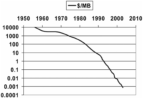
FIGURE 5.1 Decline in the price of disk space, 1950 to 2004.

disk space since the first disks in the mid-1950s, generally following the cost-performance trends of Moore’s law.

Cheaper storage led to larger and larger text collections online. Now there are many terabytes of data on the Web. These vastly larger volumes mean that precision has now become more important, since a common problem is to wade through vastly too many documents. Not surprisingly, in the mid-1980s efforts started on separating the multiple meanings of words like “bank” or “pine” and became the research area of “sense disambiguation.” 2 With sense disambiguation, it is possible to imagine searching for only one meaning of an ambiguous word, thus avoiding many erroneous retrievals.

Large-scale research on text processing took off with the availability of the TREC (Text Retrieval Evaluation Conference) data. Thanks to the National Institute of Standards and Technology, several hundred megabytes of text were provided (in each of several years) for research use. This stimulated more work on query analysis, text handling, searching

algorithms, and related areas; see the series titled TREC Conference Proceedings, edited by Donna Harmon of NIST.

Document clustering appeared as an important way to shorten long search results. Clustering enables a system to report not, say, 5000 documents but rather 10 groups of 500 documents each, and the user can then explore the group or groups that seem relevant. Salton anticipated the future possibility of such algorithms, as did others. 3 Until we got large collections, though, clustering did not find application in the document retrieval world. Now one routinely sees search engines using these techniques, and faster clustering algorithms have been developed.

Thus the algorithms explored switched from recall aids to precision aids as the quantity of available data increased. Manual thesauri, for example, have dropped out of favor for retrieval, partly because of their cost but also because their goal is to increase recall, which is not today’s problem. In terms of finding the concepts hinted at by words and phrases, our goals now are to sharpen rather than broaden these concepts: thus disambiguation and phrase matching, and not as much work on thesauri and term associations.

Again, multilingual searching started to matter, because multilingual collections became available. Multilingual research shows a more precise example of particular information resources driving research. The Canadian government made its Parliamentary proceedings (called Hansard ) available in both French and English, with paragraph-by-paragraph translation. This data stimulated a number of projects looking at how to handle bilingual material, including work on automatic alignment of the parallel texts, automatic linking of similar words in the two languages, and so on. 4

A similar effect was seen with the Brown corpus of tagged English text, where the part of speech of each word (e.g., whether a word is a noun or a verb) was identified. This produced a few years of work on algorithms that learned how to assign parts of speech to words in running text based on statistical techniques, such as the work by Garside. 5

One might see an analogy to various new fields of chemistry. The recognition that pesticides like DDT were environmental pollutants led to a new interest in biodegradability, and the Freon propellants used in aerosol cans stimulated research in reactions in the upper atmosphere. New substances stimulated a need to study reactions that previously had not been a top priority for chemistry and chemical engineering.

As storage became cheaper, image storage was now as practical as text storage had been a decade earlier. Starting in the 1980s we saw the IBM QBIC project demonstrating that something could be done to retrieve images directly, without having to index them by text words first. 6 Projects like this were stimulated by the availability of “clip art” such as the COREL image disks. Several different projects were driven by the easy access to images in this way, with technology moving on from color and texture to more accurate shape processing. At Berkeley, for example, the “Blobworld” project made major improvements in shape detection and recognition, as described in Carson et al. 7 These projects demonstrated that retrieval could be done with images as well as with words, and that properties of images could be found that were usable as concepts for searching.

Another new kind of data that became feasible to process was sound, in particular human speech. Here it was the Defense Advanced Research Projects Agency (DARPA) that took the lead, providing the SWITCH-BOARD corpus of spoken English. Again, the availability of a substantial file of tagged information helped stimulate many research projects that used this corpus and developed much of the technology that eventually went into the commercial speech recognition products we now have. As with the TREC contests, the competitions run by DARPA based on its spoken language data pushed the industry and the researchers to new advances. National needs created a new technology; one is reminded of the development of synthetic rubber during World War II or the advances in catalysis needed to make explosives during World War I.

Yet another kind of new data was geo-coded data, introducing a new set of conceptual ideas related to place. Geographical data started showing up in machine-readable form during the 1980s, especially with the release of the Dual Independent Map Encoding (DIME) files after the 1980

census and the Topologically Integrated Geographic Encoding and Referencing (TIGER) files from the 1990 census. The availability, free of charge, of a complete U.S. street map stimulated much research on systems to display maps, to give driving directions, and the like. 8 When aerial photographs also became available, there was the triumph of Microsoft’s “Terraserver,” which made it possible to look at a wide swath of the world from the sky along with correlated street and topographic maps. 9

More recently, in the 1990s, we have started to look at video search and retrieval. After all, if a CD-ROM contains about 300,000 times as many bytes per pound as a deck of punched cards, and a digitized video has about 500,000 times as many bytes per second as the ASCII script it comes from, we should be about where we were in the 1960s with video today. And indeed there are a few projects, most notably the Informedia project at Carnegie Mellon University, that experiment with video signals; they do not yet have ways of searching enormous collections, but they are developing algorithms that exploit whatever they can find in the video: scene breaks, closed-captioning, and so on.

Again, there is the problem of deducing concepts from a new kind of information. We started with the problem of words in one language needing to be combined when synonymous, picked apart when ambiguous, and moved on to detecting synonyms across multiple languages and then to concepts depicted in pictures and sounds. Now we see research such as that by Jezekiel Ben-Arie associating words like “run” or “hop” with video images of people doing those actions. In the same way we get again new chemistry when molecules like “buckyballs” are created and stimulate new theoretical and reaction studies.

Defining concepts for search can be extremely difficult. For example, despite our abilities to parse and define every item in a computer language, we have made no progress on retrieval of software; people looking for search or sort routines depend on metadata or comments. Some areas seem more flexible than others: text and naturalistic photograph processing software tends to be very general, while software to handle CAD diagrams and maps tends to be more specific. Algorithms are sometimes portable; both speech processing and image processing need Fourier transforms, but the literature is less connected than one might like (partly

because of the difference between one-dimensional and two-dimensional transforms).

There are many other examples of interesting computer science research stimulated by the availability of particular kinds of information. Work on string matching today is often driven by the need to align sequences in either protein or DNA data banks. Work on image analysis is heavily influenced by the need to deal with medical radiographs. And there are many other interesting projects specifically linked to an individual data source. Among examples:

The British Library scanning of the original manuscript of Beowulf in collaboration with the University of Kentucky, working on image enhancement until the result of the scanning is better than reading the original;

The Perseus project, demonstrating the educational applications possible because of the earlier Thesaurus Linguae Graecae project, which digitized all the classical Greek authors;

The work in astronomical analysis stimulated by the Sloan Digital Sky Survey;

The creation of the field of “forensic paleontology” at the University of Texas as a result of doing MRI scans of fossil bones;

And, of course, the enormous amount of work on search engines stimulated by the Web.

When one of these fields takes off, and we find wide usage of some online resource, it benefits society. Every university library gained readers as their catalogs went online and became accessible to students in their dorm rooms. Third World researchers can now access large amounts of technical content their libraries could rarely acquire in the past.

In computer science, and in chemistry, there is a tension between the algorithm/reaction and the data/substance. For example, should one look up an answer or compute it? Once upon a time logarithms were looked up in tables; today we also compute them on demand. Melting points and other physical properties of chemical substances are looked up in tables; perhaps with enough quantum mechanical calculation we could predict them, but it’s impractical for most materials. Predicting tomorrow’s weather might seem a difficult choice. One approach is to measure the current conditions, take some equations that model the atmosphere, and calculate forward a day. Another is to measure the current conditions, look in a big database for the previous day most similar to today, and then take the day after that one as the best prediction for tomorrow. However, so far the meteorologists feel that calculation is better. Another complicated example is chess: given the time pressure of chess tournaments

against speed and storage available in computers, chess programs do the opening and the endgame by looking in tables of old data and calculate for the middle game.

To conclude, a recipe for stimulating advances in computer science is to make some data available and let people experiment with it. With the incredibly cheap disks and scanners available today, this should be easier than ever. Unfortunately, what we gain with technology we are losing to law and economics. Many large databases are protected by copyright; few motion pictures, for example, are old enough to have gone out of copyright. Content owners generally refuse to grant permission for wide use of their material, whether out of greed or fear: they may have figured out how to get rich off their files of information or they may be afraid that somebody else might have. Similarly it is hard to get permission to digitize in-copyright books, no matter how long they have been out of print. Jim Gray once said to me, “May all your problems be technical.” In the 1960s I was paying people to key in aeronautical abstracts. It never occurred to us that we should be asking permission of the journals involved (I think what we did would qualify as fair use, but we didn’t even think about it). Today I could scan such things much more easily, but I would not be able to get permission. Am I better off or worse off?

There are now some 22 million chemical substances in the Chemical Abstracts Service Registry and 7 million reactions. New substances continue to intrigue chemists and cause research on new reactions, with of course enormous interest in biochemistry both for medicine and agriculture. Similarly, we keep adding data to the Web, and new kinds of information (photographs of dolphins, biological flora, and countless other things) can push computer scientists to new algorithms. In both cases, synthesis of specific instances into concepts is a crucial problem. As we see more and more kinds of data, we learn more about how to extract meaning from it, and how to present it, and we develop a need for new algorithms to implement this knowledge. As the data gets bigger, we learn more about optimization. As it gets more complex, we learn more about representation. And as it gets more useful, we learn more about visualization and interfaces, and we provide better service to society.

HISTORY AND THE FUNDAMENTALS OF COMPUTER SCIENCE

Edward L. Ayers, University of Virginia

We might begin with a thought experiment: What is history? Many people, I’ve discovered, think of it as books and the things in books. That’s certainly the explicit form in which we usually confront history. Others, thinking less literally, might think of history as stories about the past; that would open us to oral history, family lore, movies, novels, and the other forms in which we get most of our history.

All these images are wrong, of course, in the same way that images of atoms as little solar systems are wrong, or pictures of evolution as profiles of ever taller and more upright apes and people are wrong. They are all models, radically simplified, that allow us to think about such things in the exceedingly small amounts of time that we allot to these topics.

The same is true for history, which is easiest to envision as technological progress, say, or westward expansion, of the emergence of freedom—or of increasing alienation, exploitation of the environment, or the growth of intrusive government.

Those of us who think about specific aspects of society or nature for a living, of course, are never satisfied with the stories that suit the purposes of everyone else so well.

We are troubled by all the things that don’t fit, all the anomalies, variance, and loose ends. We demand more complex measurement, description, and fewer smoothing metaphors and lowest common denominators.

Thus, to scientists, atoms appear as clouds of probability; evolution appears as a branching, labyrinthine bush in which some branches die out and others diversify. It can certainly be argued that past human experience is as complex as anything in nature and likely much more so, if by complexity we mean numbers of components, variability of possibilities, and unpredictability of outcomes.

Yet our means of conveying that complexity remain distinctly analog: the story, the metaphor, the generalization. Stories can be wonderfully complex, of course, but they are complex in specific ways: of implication, suggestion, evocation. That’s what people love and what they remember.

But maybe there is a different way of thinking about the past: as information. In fact, information is all we have. Studying the past is like studying scientific processes for which you have the data but cannot run the experiment again, in which there is no control, and in which you can never see the actual process you are describing and analyzing. All we have is information in various forms: words in great abundance, billions of numbers, millions of images, some sounds and buildings, artifacts.

The historian’s goal, it seems to me, should be to account for as much of the complexity embedded in that information as we can. That, it appears, is what scientists do, and it has served them well.

And how has science accounted for ever-increasing amounts of complexity in the information they use? Through ever more sophisticated instruments. The connection between computer science and history could be analogous to that between telescopes and stars, microscopes and cells. We could be on the cusp of a new understanding of the patterns of complexity in human behavior of the past.

The problem may be that there is too much complexity in that past, or too much static, or too much silence. In the sciences, we’ve learned how to filter, infer, use indirect evidence, and fill in the gaps, but we have a much more literal approach to the human past.

We have turned to computer science for tasks of more elaborate description, classification, representation. The digital archive my colleagues and I have built, the Valley of the Shadow Project, permits the manipulation of millions of discrete pieces of evidence about two communities in the era of the American Civil War. It uses sorting mechanisms, hypertextual display, animation, and the like to allow people to handle the evidence of this part of the past for themselves. This isn’t cutting-edge computer science, of course, but it’s darned hard and deeply disconcerting to some, for it seems to abdicate responsibility, to undermine authority, to subvert narrative, to challenge story.

Now, we’re trying to take this work to the next stage, to analysis. We have composed a journal article that employs an array of technologies, especially geographic information systems and statistical analysis in the creation of the evidence. The article presents its argument, evidence, and historiographical context as a complex textual, tabular, and graphical representation. XML offers a powerful means to structure text and XSL an even more powerful means to transform it and manipulate its presentation. The text is divided into sections called “statements,” each supported with “explanation.” Each explanation, in turn, is supported by evidence and connected to relevant historiography.

Linkages, forward and backward, between evidence and narrative are central. The historiography can be automatically sorted by author, date, or title; the evidence can be arranged by date, topic, or type. Both evidence and historiographical entries are linked to the places in the analysis where they are invoked. The article is meant to be used online, but it can be printed in a fixed format with all the limitations and advantages of print.

So, what are the implications of thinking of the past in the hardheaded sense of admitting that all we really have of the past is information? One implication might be great humility, since all we have for most

of the past are the fossils of former human experience, words frozen in ink and images frozen in line and color. Another implication might be hubris: if we suddenly have powerful new instruments, might we be on the threshold of a revolution in our understanding of the past? We’ve been there before.

A connection between history and social science was tried before, during the first days of accessible computers. Historians taught themselves statistical methods and even programming languages so that they could adopt the techniques, models, and insights of sociology and political science. In the 1950s and 1960s the creators of the new political history called on historians to emulate the precision, explicitness, replicability, and inclusivity of the quantitative social sciences. For two decades that quantitative history flourished, promising to revolutionize the field. And to a considerable extent it did: it changed our ideas of social mobility, political identification, family formation, patterns of crime, economic growth, and the consequences of ethnic identity. It explicitly linked the past to the present and held out a history of obvious and immediate use.

But that quantitative social science history collapsed suddenly, the victim of its own inflated claims, limited method and machinery, and changing academic fashion. By the mid-1980s, history, along with many of the humanities and social sciences, had taken the linguistic turn. Rather than software manuals and codebooks, graduate students carried books of French philosophy and German literary interpretation. The social science of choice shifted from sociology to anthropology; texts replaced tables. A new generation defined itself in opposition to social scientific methods just as energetically as an earlier generation had seen in those methods the best means of writing a truly democratic history. The first computer revolution largely failed.

The first effort at that history fell into decline in part because historians could not abide the distance between their most deeply held beliefs and what the statistical machinery permitted, the abstraction it imposed. History has traditionally been built around contingency and particularity, but the most powerful tools of statistics are built on sampling and extrapolation, on generalization and tendency. Older forms of social history talked about vague and sometimes dubious classifications in part because that was what the older technology of tabulation permitted us to see. It has become increasingly clear across the social sciences that such flat ways of describing social life are inadequate; satisfying explanations must be dynamic, interactive, reflexive, and subtle, refusing to reify structures of social life or culture. The new technology permits a new cross-fertilization.

Ironically, social science history faded just as computers became widely available, just as new kinds of social science history became feasible. No longer is there any need for white-coated attendants at huge mainframes

and expensive proprietary software. Rather than reducing people to rows and columns, searchable databases now permit researchers to maintain the identities of individuals in those databases and to represent entire populations rather than samples. Moreover, the record can now include things social science history could only imagine before the Web: completely indexed newspapers, with the original readable on the screen; completely searchable letters and diaries by the thousands; and interactive maps with all property holders identified and linked to other records. Visualization of patterns in the data, moreover, far outstrips the possibilities of numerical calculation alone. Manipulable histograms, maps, and time lines promise a social history that is simultaneously sophisticated and accessible. We have what earlier generations of social science historians dreamed of: a fast and widely accessible network linked to cheap and powerful computers running common software with well-established standards for the handling of numbers, texts, and images. New possibilities of collaboration and cumulative research beckon. Perhaps the time is right to reclaim a worthy vision of a disciplined and explicit social scientific history that we abandoned too soon.

What does this have to do with computer science? Everything, it seems to me. If you want hard problems, historians have them. And what’s the hardest problem of all right now? The capture of the very information that is history. Can computer science imagine ways to capture historical information more efficiently? Can it offer ways to work with the spotty, broken, dirty, contradictory, nonstandardized information we work with?

The second hard problem is the integration of this disparate evidence in time and space, offering new precision, clarity, and verifiability, as well as opening new questions and new ways of answering them.

If we can think of these ways, then we face virtually limitless possibilities. Is there a more fundamental challenge or opportunity for computer science than helping us to figure out human society over human time?

This page intentionally left blank.

Computer Science: Reflections on the Field, Reflections from the Field provides a concise characterization of key ideas that lie at the core of computer science (CS) research. The book offers a description of CS research recognizing the richness and diversity of the field. It brings together two dozen essays on diverse aspects of CS research, their motivation and results. By describing in accessible form computer science’s intellectual character, and by conveying a sense of its vibrancy through a set of examples, the book aims to prepare readers for what the future might hold and help to inspire CS researchers in its creation.

READ FREE ONLINE

Welcome to OpenBook!

You're looking at OpenBook, NAP.edu's online reading room since 1999. Based on feedback from you, our users, we've made some improvements that make it easier than ever to read thousands of publications on our website.

Do you want to take a quick tour of the OpenBook's features?

Show this book's table of contents , where you can jump to any chapter by name.

...or use these buttons to go back to the previous chapter or skip to the next one.

Jump up to the previous page or down to the next one. Also, you can type in a page number and press Enter to go directly to that page in the book.

Switch between the Original Pages , where you can read the report as it appeared in print, and Text Pages for the web version, where you can highlight and search the text.

To search the entire text of this book, type in your search term here and press Enter .

Share a link to this book page on your preferred social network or via email.

View our suggested citation for this chapter.

Ready to take your reading offline? Click here to buy this book in print or download it as a free PDF, if available.

Get Email Updates

Do you enjoy reading reports from the Academies online for free ? Sign up for email notifications and we'll let you know about new publications in your areas of interest when they're released.

CHAPTER 4: DATA MEASUREMENT

4-3: Types of Data and Appropriate Representations

Introduction.

Graphs and charts can be effective visual tools because they present information quickly and easily. Graphs and charts condense large amounts of information into easy-to-understand formats that clearly and effectively communicate important points. Graphs are commonly used by print and electronic media as they quickly convey information in a small space. Statistics are often presented visually as they can effectively facilitate understanding of the data. Different types of graphs and charts are used to represent different types of data.

  Types of Data

There are four types of data used in statistics: nominal data, ordinal data, discrete data, and continuous data. Nominal and ordinal data fall under the umbrella of categorical data, while discrete data and continuous data fall under the umbrella of continuous data.

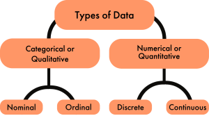
Qualitative Data

Categorical or qualitative data labels data into categories. Categorical data is defined in terms of natural language specifications. For example, name, sex, country of origin, are categories that represent qualitative data. There are two subcategories of qualitative data, nominal data and ordinal data.

Nominal Data

Ordinal Data

When the categories have a natural order, the categories are said to be ordinal . It can be ordered and measured. For example education level (H.S. diploma; 1 year certificate; 2 year degree; 4 year degree; masters degree; doctorate degree), satisfaction rating (extremely dislike; dislike; neutral; like; extremely like), etc. are categories that have a natural order to them. Ordinal data are commonly used for collecting demographic information (age, sex, race, etc.). This is particularly prevalent in marketing and insurance sectors, but it is also used by governments (e.g. the census), and is commonly used when conducting customer satisfaction surveys. Ordinal data is commonly represented using a bar graph .

Quantitative Data

Quantitative data has two subcategories, discrete data and continuous data.

Discrete Data

The data is discrete when the numbers do not touch each other on a real number line (e.g., 0, 1, 2, 3, 4…). Discrete data is whole numerical values typically shown as counts and contains only a finite number of possible values. For example, the number of visits to the doctor, the number of students in a class, etc. Discrete data is typically represented by a histogram .

Continuous Data

The data is continuous when it has an infinite number of possible values that can be selected within certain limits. (i.e., the numbers run into each other on a real number line). Continuous data is data that can be calculated . It has an infinite number of possible values that can be selected within certain limits. Examples of continuous data are temperature, time, height, etc. Continuous data is typically represented by a line graph .

Explore 1 – Types of data

Classify the data into qualitative or quantitative, then into a subcategory of nominal, ordinal, discrete or continuous.

Weight is a number that is measured and has order. It can also take on any number. So, weight is quantitative: continuous.

• egg size (small, medium, large, extra large)

Egg size is typically small, medium, large, or extra large that has a natural order. So, egg size is qualitative: ordinal.

• number of miles driven to work

Number of miles is a number that is measured and has order. It can also take on any number. So, number of miles is : quantitative: continuous.

• body temperature

Body temperature is a number that is measured and has order. It can also take on any number. So, temperature is quantitative: continuous.

• basketball team jersey number

Jersey numbers have no order and are numbers that are not measured. So, jersey number is qualitative: nominal.

• U.S. shoe size

Shoe size is a number. It is calculated based on a formula that includes the measure of your foot length. However, it has only whole or half numbers (e.g., 8 or 9.5). Shoe size has a natural order but has a finite number of options (e.g., half or whole numbers). So, shoe size is quantitative: discrete.

• military rank

Military rank is not numerical but is categorical with a natural order. So, military rank is qualitative: ordinal.

• university GPA

University GPA is a weighted average that is calculated, so it is quantitative: continuous.

Practice Exercises

• year of birth
• levels of fluency (language)
• height of players on a team
• dose of medicine
• political party
• course letter grades
• Quantitative: discrete
• Qualitative: ordinal
• Quantitative: continuous
• Qualitative: nominal

Types of Graphs and Charts

The type of graph or chart used to visualize data is determined by the type of data being represented. A pie chart or bar chart  is typically used for nominal data and a bar chart for ordinal data . For quantitative data , we typically use a histogram for discrete data and a line graph for continuous data .

A pie chart is a circular graphic which is divided into slices to illustrate numerical proportion. Pie charts are widely used in the business world and the mass media. The size of each slice is determined by the percentage represented by a category compared to the whole (i.e., the entire dataset). The percentage in each category adds to 100% or the whole.  

Explore 2 – Pie Charts

The pie chart shows the distribution of the Food and Drug Administration’s Budget of different programs for the fiscal year 2021. The total  budget was $6.1 billion. [1]

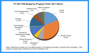
• How many categories are shown in the pie chart?

If we count the number of slices, there are 10 categories shown.

• What do the percentages represent?

The percentages show the percent of the $6.1 billion FDA budget that was spent on each category.

• Why is it vital to show the total budget on the chart?

Without the total budget we would be unable to calculate the amount spent on each category.

• Is there a limit to the number of categories that can be shown on a pie chart?

Yes. If the slices are too small to see, another method of representing the data should be used. Ideally, a pie chart should show no more than 5 or 6 categories.

• What does the largest slice represent?

The percentage of the total budget spent on human drugs.

• What does the smallest slice represent?

The percentage of the total budget spent on toxicological research.

• How could this pie chart be improved?

The slices could be ordered around the circle by size, and the 3-D look could be eliminated to avoid the distorted perspective and to make the graph clearer.

• Is this an appropriate use of a pie chart?

The chart is showing a comparison of all categories the budget went towards so it is appropriate.

Bar graphs are used to represent categorical data . Each category is represented as a bar either vertically or horizontally. A bar is the measured value or percentage of a category and there is equal space between each pair of consecutive bars. Bar graphs have the advantage of being easy to read and offer direct comparison of categories. 

Explore 3 – Bar Graphs

Graduation rates within 6 years from the first institution attended for first-time, full-time bachelor’s degree-seeking students at 4-year postsecondary institutions, by race/ethnicity: cohort entry year 2010.

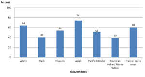
• How many categories are represented in the bar graph and what do they represent?

There are 7 categories representing the race/ethnicity of the students.

• What do the numbers above each bar represent and why may they be necessary?

The rounded percent of the category. They are necessary because it is very difficult to tell from the vertical scale the height of each bar.

• What does the tallest bar represent?

The percent of students who graduated within six years from their first institution within 6 years who were Asian.

• What does the shortest bar represent?

The percent of students who graduated within six years from their first institution within 6 years who were American Indian or Alaska Native.

• Is this an appropriate use of a bar graph?

Yes. The data is qualitative: nominal; there is no order within the categories.

Histograms are used to represent quantitative data that is discrete . A histogram divides up the range of possible values in a data set into classes or intervals. For each class, a rectangle is constructed with a base length equal to the range of values in that specific class and a length equal to the number of observations falling into that class. A histogram has an appearance similar to a vertical bar chart, but there are no gaps between the bars. The bars are ordered along the axis from the smallest to the largest possible value. Consequently, the bars cannot be reordered. Histograms are often used to illustrate the major features of the distribution of the data in a convenient form. They are also useful when dealing with large data sets (greater than 100 observations). They can help detect any unusual observations (outliers) or any gaps in the data.

Histograms may look similar to bar charts but they are really completely different. Histograms plot quantitative data with ranges of the data grouped into classes or intervals while bar charts plot categorical data. Histograms are used to show distributions while bar charts are used to compare categories. Bars can be reordered in bar charts but not in histograms. The bars of bar charts have the same width. The widths of the bars in a histogram need not be the same as long as the total area of all bars is one hundred percent if percentages are used or the total count, if counts are used. Therefore, values in bar graphs are given by the length of the bar while values in histograms are given by areas.

Explore 4 – Histograms

Reading data from a table can be less than enlightening and certainly doesn’t inspire much interest. Graphing the same data in a histogram gives a graphical representation where certain features are automatically highlighted.

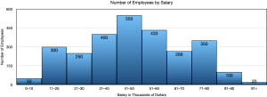
• What do you notice about the bars of this histogram compared to the bars of a bar graph?

The bars touch in a histogram but not in a bar chart. This is because the data is ordered along the axis.

• What do the numbers above the bars represent?

The number of employees whose salary lands in each class.

• State a feature of the graph that is very obvious to you.

Answers may vary. Very few employees make less than $10,000 or more than $91,000. $41,000 – $50,000 is the most common salary.

Line graphs are used when the data is quantitative and continuous . The axis acts as a real number line where every possible value is located. Line graphs are typically used to show how data values change over time.

Explore 5 – Line Graphs

Here is an example of a line graph.

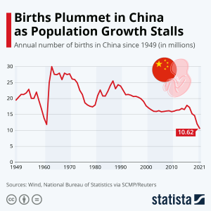
• What does this line graph represent?

Solution:  The number of annual births in China from 1949 to 2021.

• What do the numbers on the vertical axis represent?

Solution:  The number of births in millions.

• What do the numbers on the horizontal axis represent?

Solution:  The year.

• Is this an appropriate use of a line graph?

Solution:  Yes. The time scale in years is continuous and a line graph is appropriate for continuous data.

• Does a line graph highlight anything that a histogram may not?

Solution:  Yes. The trend in data over time. In this graph the trend of annual births is decreasing.

Infographics are often used by media outlets who are trying to tell a specific (often biased) story. They often combine charts or graphs with narrative and statistics.

Explore 6 – Infographics

Solution:  Since it is circular and based on percentages in each category, it is based on a pie chart.

• How many categories are represented?

Solution:  There are three categories.

• What story is the infographic trying to tell?

Solution:  About one third of Americans believe in aliens.

• How was the data gathered?

Solution:  A survey of 1522 U.S. adults.

• What does the largest blue area on the chart represent?

Solution:  The percentage of those surveyed that believe that all sightings can be explained by human activity or natural phenomena.

• What does the smallest grey area on the chart represent?

Solution:  The percentage of those surveyed that have no opinion on UFO sightings.

• Robert is involved in a group project for a class. The group has collected data to show the amount of time spent performing different tasks on a cell phone. The categories include making calls, Internet, text, music, videos, social media, email, games, and photos. What type of graph or chart should be used to display the average time spent per day on any of these tasks? Explain your reasoning.  
• A marketing firm wants to show what fraction of the overall market uses a particular Internet browser. What type of graph or chart should be used to display this information? Explain your reasoning.  
• The data is categorical so a bar graph should be used.
• The data is categorical. If there are not too many categories (browser used) then a pie chart would work since fraction of the market is used. Alternatively, a bar chart could be used showing the fraction or percent as the height of each bar.

• Name three (3) differences between a bar graph and a histogram.
• A bar graph is used for qualitative data while a histogram is used for quantitative data.
• In a bar graph the categories can be reordered. In a histogram the categories cannot be reordered.
• In a bar graph the bars do not touch. In a histogram the bars touch.
• A teacher wants to show their class the results of a midterm exam, without exposing any student names. What type of graph or chart should be used to display the scores earned on the midterm? Explain your reasoning.  
• A pizza company wants to display a graphic of the five favorite pizzas of their customers on the company website. What type of graph or chart should be used to display this information? Explain your reasoning.  
• Maria is keeping track of her daughter’s height by measuring her height on her birthday each year and recording it in a spreadsheet. What type of graph or chart should be used to display this information? Explain your reasoning
• Midterm scores may be quantitative as either raw scores or percentages, in which case they should show a histogram showing the number of students scoring in a given score (or percentage) interval. If the midterm results are letter grades, the data is qualitative but ordered. In this case, a pie chart could be used to show the percent of students with each letter grade, but it would be very busy.  A better option would be a bar graph showing the number of students at each letter grade.
• An infographic. This is categorical data so a (pizza) pie chart would be a good option or a bar chart.
• A line graph since the data is collected over time and time is continuous.

Perspectives

• Mike has collected data for a school project from a survey that asked, “What is your favorite pizza? ”. He surveyed 200 people and discovered that there were only 9 pizzas that were on the favorites list. In his report, he plans to show his data in a (pizza) pie chart. Is this the correct chart to use for his purpose? Explain your reasoning.  
• Sarah is keeping track of the value of her car every year. She started when she first bought the car new and looks up its value every year. She figures that when the car’s value drops to $5000, it is time for an upgrade. What type of graph or chart should be used to display this information? Explain your reasoning.  
• The Earth’s atmosphere is made up of 77% Nitrogen, 21% Oxygen, and 2% other gases. What type of graph or chart should be used to display this data? Explain your reasoning.  
• A pie chart could be used but with 9 categories there may be too many slices for the chart to be clear. A bar graph may be better due to the number of categories.
• A line graph since time is continuous and she will be able to see the trend in car value over time.
• The data is qualitative: nominal and has percentages that add to 100% so a pie chart would work well with only 3 categories. Alternatively, a bar chart would work.

Skills Exercises

• phone number
• https://www.fda.gov/about-fda/fda-basics/fact-sheet-fda-glance ↵

able to be put into categories

data that can be given labels and put into categories

qualitative data that can be put into labelled categories that have no order and no overlap

having nothing in common; no overlap

the number of times a data value has been recorded

a number or ratio expressed as a fraction of 100

a circular graphic which is divided into slices representing the number or percentage in each category

qualitative data that has a natural order

a graph where each category is represented by a vertical or horizontal bar that measures a frequency or percentage of the whole

expressed using a number or numbers

data that involves numerical values with order

data that is measured using whole numbers with only a finite number of possibilities

a graph similar in appearance to a vertical bar graph with gaps between the bars, ordered bars, with a bse length equal to the range of values in a specific class

data that has an infinite number of possible values that can be selected within certain limits

use arithmetic and the order of operations

a graph used for continuous data that uses an axis as a real number line where every possible value is located

a graphic showing a combination of graphs, charts, and statistics

Numeracy Copyright © 2023 by Utah Valley University is licensed under a Creative Commons Attribution-NonCommercial-ShareAlike 4.0 International License , except where otherwise noted.

• Skip to main content
• Skip to primary sidebar
• Skip to footer
• QuestionPro

• Solutions Industries Gaming Automotive Sports and events Education Government Travel & Hospitality Financial Services Healthcare Cannabis Technology Use Case NPS+ Communities Audience Contactless surveys Mobile LivePolls Member Experience GDPR Positive People Science 360 Feedback Surveys
• Resources Blog eBooks Survey Templates Case Studies Training Help center

Home Market Research

Data Analysis in Research: Types & Methods

Content Index

Why analyze data in research?

Types of data in research, finding patterns in the qualitative data, methods used for data analysis in qualitative research, preparing data for analysis, methods used for data analysis in quantitative research, considerations in research data analysis, what is data analysis in research.

Definition of research in data analysis: According to LeCompte and Schensul, research data analysis is a process used by researchers to reduce data to a story and interpret it to derive insights. The data analysis process helps reduce a large chunk of data into smaller fragments, which makes sense. 

Three essential things occur during the data analysis process — the first is data organization . Summarization and categorization together contribute to becoming the second known method used for data reduction. It helps find patterns and themes in the data for easy identification and linking. The third and last way is data analysis – researchers do it in both top-down and bottom-up fashion.

LEARN ABOUT: Research Process Steps

On the other hand, Marshall and Rossman describe data analysis as a messy, ambiguous, and time-consuming but creative and fascinating process through which a mass of collected data is brought to order, structure and meaning.

We can say that “the data analysis and data interpretation is a process representing the application of deductive and inductive logic to the research and data analysis.”

Researchers rely heavily on data as they have a story to tell or research problems to solve. It starts with a question, and data is nothing but an answer to that question. But, what if there is no question to ask? Well! It is possible to explore data even without a problem – we call it ‘Data Mining’, which often reveals some interesting patterns within the data that are worth exploring.

Irrelevant to the type of data researchers explore, their mission and audiences’ vision guide them to find the patterns to shape the story they want to tell. One of the essential things expected from researchers while analyzing data is to stay open and remain unbiased toward unexpected patterns, expressions, and results. Remember, sometimes, data analysis tells the most unforeseen yet exciting stories that were not expected when initiating data analysis. Therefore, rely on the data you have at hand and enjoy the journey of exploratory research. 

Create a Free Account

Every kind of data has a rare quality of describing things after assigning a specific value to it. For analysis, you need to organize these values, processed and presented in a given context, to make it useful. Data can be in different forms; here are the primary data types.

• Qualitative data: When the data presented has words and descriptions, then we call it qualitative data . Although you can observe this data, it is subjective and harder to analyze data in research, especially for comparison. Example: Quality data represents everything describing taste, experience, texture, or an opinion that is considered quality data. This type of data is usually collected through focus groups, personal qualitative interviews , qualitative observation or using open-ended questions in surveys.
• Quantitative data: Any data expressed in numbers of numerical figures are called quantitative data . This type of data can be distinguished into categories, grouped, measured, calculated, or ranked. Example: questions such as age, rank, cost, length, weight, scores, etc. everything comes under this type of data. You can present such data in graphical format, charts, or apply statistical analysis methods to this data. The (Outcomes Measurement Systems) OMS questionnaires in surveys are a significant source of collecting numeric data.
• Categorical data: It is data presented in groups. However, an item included in the categorical data cannot belong to more than one group. Example: A person responding to a survey by telling his living style, marital status, smoking habit, or drinking habit comes under the categorical data. A chi-square test is a standard method used to analyze this data.

Learn More : Examples of Qualitative Data in Education

Data analysis in qualitative research

Data analysis and qualitative data research work a little differently from the numerical data as the quality data is made up of words, descriptions, images, objects, and sometimes symbols. Getting insight from such complicated information is a complicated process. Hence it is typically used for exploratory research and data analysis .

Although there are several ways to find patterns in the textual information, a word-based method is the most relied and widely used global technique for research and data analysis. Notably, the data analysis process in qualitative research is manual. Here the researchers usually read the available data and find repetitive or commonly used words. 

For example, while studying data collected from African countries to understand the most pressing issues people face, researchers might find  “food”  and  “hunger” are the most commonly used words and will highlight them for further analysis.

LEARN ABOUT: Level of Analysis

The keyword context is another widely used word-based technique. In this method, the researcher tries to understand the concept by analyzing the context in which the participants use a particular keyword.  

For example , researchers conducting research and data analysis for studying the concept of ‘diabetes’ amongst respondents might analyze the context of when and how the respondent has used or referred to the word ‘diabetes.’

The scrutiny-based technique is also one of the highly recommended  text analysis  methods used to identify a quality data pattern. Compare and contrast is the widely used method under this technique to differentiate how a specific text is similar or different from each other. 

For example: To find out the “importance of resident doctor in a company,” the collected data is divided into people who think it is necessary to hire a resident doctor and those who think it is unnecessary. Compare and contrast is the best method that can be used to analyze the polls having single-answer questions types .

Metaphors can be used to reduce the data pile and find patterns in it so that it becomes easier to connect data with theory.

Variable Partitioning is another technique used to split variables so that researchers can find more coherent descriptions and explanations from the enormous data.

LEARN ABOUT: Qualitative Research Questions and Questionnaires

There are several techniques to analyze the data in qualitative research, but here are some commonly used methods,

• Content Analysis:  It is widely accepted and the most frequently employed technique for data analysis in research methodology. It can be used to analyze the documented information from text, images, and sometimes from the physical items. It depends on the research questions to predict when and where to use this method.
• Narrative Analysis: This method is used to analyze content gathered from various sources such as personal interviews, field observation, and  surveys . The majority of times, stories, or opinions shared by people are focused on finding answers to the research questions.
• Discourse Analysis:  Similar to narrative analysis, discourse analysis is used to analyze the interactions with people. Nevertheless, this particular method considers the social context under which or within which the communication between the researcher and respondent takes place. In addition to that, discourse analysis also focuses on the lifestyle and day-to-day environment while deriving any conclusion.
• Grounded Theory:  When you want to explain why a particular phenomenon happened, then using grounded theory for analyzing quality data is the best resort. Grounded theory is applied to study data about the host of similar cases occurring in different settings. When researchers are using this method, they might alter explanations or produce new ones until they arrive at some conclusion.

LEARN ABOUT: 12 Best Tools for Researchers

Data analysis in quantitative research

The first stage in research and data analysis is to make it for the analysis so that the nominal data can be converted into something meaningful. Data preparation consists of the below phases.

Phase I: Data Validation

Data validation is done to understand if the collected data sample is per the pre-set standards, or it is a biased data sample again divided into four different stages

• Fraud: To ensure an actual human being records each response to the survey or the questionnaire
• Screening: To make sure each participant or respondent is selected or chosen in compliance with the research criteria
• Procedure: To ensure ethical standards were maintained while collecting the data sample
• Completeness: To ensure that the respondent has answered all the questions in an online survey. Else, the interviewer had asked all the questions devised in the questionnaire.

Phase II: Data Editing

More often, an extensive research data sample comes loaded with errors. Respondents sometimes fill in some fields incorrectly or sometimes skip them accidentally. Data editing is a process wherein the researchers have to confirm that the provided data is free of such errors. They need to conduct necessary checks and outlier checks to edit the raw edit and make it ready for analysis.

Phase III: Data Coding

Out of all three, this is the most critical phase of data preparation associated with grouping and assigning values to the survey responses . If a survey is completed with a 1000 sample size, the researcher will create an age bracket to distinguish the respondents based on their age. Thus, it becomes easier to analyze small data buckets rather than deal with the massive data pile.

LEARN ABOUT: Steps in Qualitative Research

After the data is prepared for analysis, researchers are open to using different research and data analysis methods to derive meaningful insights. For sure, statistical analysis plans are the most favored to analyze numerical data. In statistical analysis, distinguishing between categorical data and numerical data is essential, as categorical data involves distinct categories or labels, while numerical data consists of measurable quantities. The method is again classified into two groups. First, ‘Descriptive Statistics’ used to describe data. Second, ‘Inferential statistics’ that helps in comparing the data .

Descriptive statistics

This method is used to describe the basic features of versatile types of data in research. It presents the data in such a meaningful way that pattern in the data starts making sense. Nevertheless, the descriptive analysis does not go beyond making conclusions. The conclusions are again based on the hypothesis researchers have formulated so far. Here are a few major types of descriptive analysis methods.

Measures of Frequency

• Count, Percent, Frequency
• It is used to denote home often a particular event occurs.
• Researchers use it when they want to showcase how often a response is given.

Measures of Central Tendency

• Mean, Median, Mode
• The method is widely used to demonstrate distribution by various points.
• Researchers use this method when they want to showcase the most commonly or averagely indicated response.

Measures of Dispersion or Variation

• Range, Variance, Standard deviation
• Here the field equals high/low points.
• Variance standard deviation = difference between the observed score and mean
• It is used to identify the spread of scores by stating intervals.
• Researchers use this method to showcase data spread out. It helps them identify the depth until which the data is spread out that it directly affects the mean.

Measures of Position

• Percentile ranks, Quartile ranks
• It relies on standardized scores helping researchers to identify the relationship between different scores.
• It is often used when researchers want to compare scores with the average count.

For quantitative research use of descriptive analysis often give absolute numbers, but the in-depth analysis is never sufficient to demonstrate the rationale behind those numbers. Nevertheless, it is necessary to think of the best method for research and data analysis suiting your survey questionnaire and what story researchers want to tell. For example, the mean is the best way to demonstrate the students’ average scores in schools. It is better to rely on the descriptive statistics when the researchers intend to keep the research or outcome limited to the provided  sample  without generalizing it. For example, when you want to compare average voting done in two different cities, differential statistics are enough.

Descriptive analysis is also called a ‘univariate analysis’ since it is commonly used to analyze a single variable.

Inferential statistics

Inferential statistics are used to make predictions about a larger population after research and data analysis of the representing population’s collected sample. For example, you can ask some odd 100 audiences at a movie theater if they like the movie they are watching. Researchers then use inferential statistics on the collected  sample  to reason that about 80-90% of people like the movie. 

Here are two significant areas of inferential statistics.

• Estimating parameters: It takes statistics from the sample research data and demonstrates something about the population parameter.
• Hypothesis test: I t’s about sampling research data to answer the survey research questions. For example, researchers might be interested to understand if the new shade of lipstick recently launched is good or not, or if the multivitamin capsules help children to perform better at games.

These are sophisticated analysis methods used to showcase the relationship between different variables instead of describing a single variable. It is often used when researchers want something beyond absolute numbers to understand the relationship between variables.

Here are some of the commonly used methods for data analysis in research.

• Correlation: When researchers are not conducting experimental research or quasi-experimental research wherein the researchers are interested to understand the relationship between two or more variables, they opt for correlational research methods.
• Cross-tabulation: Also called contingency tables,  cross-tabulation  is used to analyze the relationship between multiple variables.  Suppose provided data has age and gender categories presented in rows and columns. A two-dimensional cross-tabulation helps for seamless data analysis and research by showing the number of males and females in each age category.
• Regression analysis: For understanding the strong relationship between two variables, researchers do not look beyond the primary and commonly used regression analysis method, which is also a type of predictive analysis used. In this method, you have an essential factor called the dependent variable. You also have multiple independent variables in regression analysis. You undertake efforts to find out the impact of independent variables on the dependent variable. The values of both independent and dependent variables are assumed as being ascertained in an error-free random manner.
• Frequency tables: The statistical procedure is used for testing the degree to which two or more vary or differ in an experiment. A considerable degree of variation means research findings were significant. In many contexts, ANOVA testing and variance analysis are similar.
• Analysis of variance: The statistical procedure is used for testing the degree to which two or more vary or differ in an experiment. A considerable degree of variation means research findings were significant. In many contexts, ANOVA testing and variance analysis are similar.
• Researchers must have the necessary research skills to analyze and manipulation the data , Getting trained to demonstrate a high standard of research practice. Ideally, researchers must possess more than a basic understanding of the rationale of selecting one statistical method over the other to obtain better data insights.
• Usually, research and data analytics projects differ by scientific discipline; therefore, getting statistical advice at the beginning of analysis helps design a survey questionnaire, select data collection methods , and choose samples.

LEARN ABOUT: Best Data Collection Tools

• The primary aim of data research and analysis is to derive ultimate insights that are unbiased. Any mistake in or keeping a biased mind to collect data, selecting an analysis method, or choosing  audience  sample il to draw a biased inference.
• Irrelevant to the sophistication used in research data and analysis is enough to rectify the poorly defined objective outcome measurements. It does not matter if the design is at fault or intentions are not clear, but lack of clarity might mislead readers, so avoid the practice.
• The motive behind data analysis in research is to present accurate and reliable data. As far as possible, avoid statistical errors, and find a way to deal with everyday challenges like outliers, missing data, data altering, data mining , or developing graphical representation.

LEARN MORE: Descriptive Research vs Correlational Research The sheer amount of data generated daily is frightening. Especially when data analysis has taken center stage. in 2018. In last year, the total data supply amounted to 2.8 trillion gigabytes. Hence, it is clear that the enterprises willing to survive in the hypercompetitive world must possess an excellent capability to analyze complex research data, derive actionable insights, and adapt to the new market needs.

LEARN ABOUT: Average Order Value

QuestionPro is an online survey platform that empowers organizations in data analysis and research and provides them a medium to collect data by creating appealing surveys.

MORE LIKE THIS

21 Best Customer Advocacy Software for Customers in 2024

Apr 19, 2024

10 Quantitative Data Analysis Software for Every Data Scientist

Apr 18, 2024

11 Best Enterprise Feedback Management Software in 2024

17 Best Online Reputation Management Software in 2024

Apr 17, 2024

Other categories

• Academic Research
• Artificial Intelligence
• Assessments
• Brand Awareness
• Case Studies
• Communities
• Consumer Insights
• Customer effort score
• Customer Engagement
• Customer Experience
• Customer Loyalty
• Customer Research
• Customer Satisfaction
• Employee Benefits
• Employee Engagement
• Employee Retention
• Friday Five
• General Data Protection Regulation
• Insights Hub
• Life@QuestionPro
• Market Research
• Mobile diaries
• Mobile Surveys
• New Features
• Online Communities
• Question Types
• Questionnaire
• QuestionPro Products
• Release Notes
• Research Tools and Apps
• Revenue at Risk
• Survey Templates
• Training Tips
• Uncategorized
• Video Learning Series
• What’s Coming Up
• Workforce Intelligence

If you're seeing this message, it means we're having trouble loading external resources on our website.

If you're behind a web filter, please make sure that the domains *.kastatic.org and *.kasandbox.org are unblocked.

To log in and use all the features of Khan Academy, please enable JavaScript in your browser.

Praxis Core Math

Course: praxis core math   >   unit 1, data representations | lesson.

• Data representations | Worked example
• Center and spread | Lesson
• Center and spread | Worked example
• Random sampling | Lesson
• Random sampling | Worked example
• Scatterplots | Lesson
• Scatterplots | Worked example
• Interpreting linear models | Lesson
• Interpreting linear models | Worked example
• Correlation and Causation | Lesson
• Correlation and causation | Worked example
• Probability | Lesson
• Probability | Worked example

What are data representations?

• How much of the data falls within a specified category or range of values?
• What is a typical value of the data?
• How much spread is in the data?
• Is there a trend in the data over time?
• Is there a relationship between two variables?

What skills are tested?

• Matching a data set to its graphical representation
• Matching a graphical representation to a description
• Using data representations to solve problems

How are qualitative data displayed?

• A vertical bar chart lists the categories of the qualitative variable along a horizontal axis and uses the heights of the bars on the vertical axis to show the values of the quantitative variable. A horizontal bar chart lists the categories along the vertical axis and uses the lengths of the bars on the horizontal axis to show the values of the quantitative variable. This display draws attention to how the categories rank according to the amount of data within each. Example The heights of the bars show the number of students who want to study each language. Using the bar chart, we can conclude that the greatest number of students want to study Mandarin and the least number of students want to study Latin.
• A pictograph is like a horizontal bar chart but uses pictures instead of the lengths of bars to represent the values of the quantitative variable. Each picture represents a certain quantity, and each category can have multiple pictures. Pictographs are visually interesting, but require us to use the legend to convert the number of pictures to quantitative values. Example Each represents 40 ‍   students. The number of pictures shows the number of students who want to study each language. Using the pictograph, we can conclude that twice as many students want to study French as want to study Latin.
• A circle graph (or pie chart) is a circle that is divided into as many sections as there are categories of the qualitative variable. The area of each section represents, for each category, the value of the quantitative data as a fraction of the sum of values. The fractions sum to 1 ‍   . Sometimes the section labels include both the category and the associated value or percent value for that category. Example The area of each section represents the fraction of students who want to study that language. Using the circle graph, we can conclude that just under 1 2 ‍   the students want to study Mandarin and about 1 3 ‍   want to study Spanish.

How are quantitative data displayed?

• Dotplots use one dot for each data point. The dots are plotted above their corresponding values on a number line. The number of dots above each specific value represents the count of that value. Dotplots show the value of each data point and are practical for small data sets. Example Each dot represents the typical travel time to school for one student. Using the dotplot, we can conclude that the most common travel time is 10 ‍   minutes. We can also see that the values for travel time range from 5 ‍   to 35 ‍   minutes.
• Histograms divide the horizontal axis into equal-sized intervals and use the heights of the bars to show the count or percent of data within each interval. By convention, each interval includes the lower boundary but not the upper one. Histograms show only totals for the intervals, not specific data points. Example The height of each bar represents the number of students having a typical travel time within the corresponding interval. Using the histogram, we can conclude that the most common travel time is between 10 ‍   and 15 ‍   minutes and that all typical travel times are between 5 ‍   and 40 ‍   minutes.

How are trends over time displayed?

How are relationships between variables displayed.

• (Choice A)   A
• (Choice B)   B
• (Choice C)   C
• (Choice D)   D
• (Choice E)   E
• Your answer should be
• an integer, like 6 ‍  
• a simplified proper fraction, like 3 / 5 ‍  
• a simplified improper fraction, like 7 / 4 ‍  
• a mixed number, like 1   3 / 4 ‍  
• an exact decimal, like 0.75 ‍  
• a multiple of pi, like 12   pi ‍   or 2 / 3   pi ‍  
• a proper fraction, like 1 / 2 ‍   or 6 / 10 ‍  
• an improper fraction, like 10 / 7 ‍   or 14 / 8 ‍  

Things to remember

• When matching data to a representation, check that the values are graphed accurately for all categories.
• When reporting data counts or fractions, be clear whether a question asks about data within a single category or a comparison between categories.
• When finding the number or fraction of the data meeting a criteria, watch for key words such as or , and , less than , and more than .

Want to join the conversation?

• Upvote Button navigates to signup page
• Downvote Button navigates to signup page
• Flag Button navigates to signup page

Methods for Data Representation

• First Online: 21 April 2023

Cite this chapter

• Ramón Zatarain Cabada   ORCID: orcid.org/0000-0002-4524-3511 4 ,
• Héctor Manuel Cárdenas López   ORCID: orcid.org/0000-0002-6823-4933 4 &
• Hugo Jair Escalante   ORCID: orcid.org/0000-0003-4603-3513 5  

122 Accesses

This chapter provides an overview of the preprocessing techniques for preparing data for personality recognition. It begins with explaining adaptations required for handling large datasets that cannot be loaded into memory. The chapter then focuses on image preprocessing techniques in videos, including face delineation, obturation, and various techniques applied to video images. The chapter also discusses sound preprocessing, such as common sound representation techniques, spectral coefficients, prosody, and intonation. Finally, Mel spectral and delta Mel spectral coefficients are discussed as sound representation techniques for personality recognition. The primary aim of this chapter is to help readers understand different video processing techniques that can be used in data representation for personality recognition.

This is a preview of subscription content, log in via an institution to check access.

Access this chapter

• Available as PDF
• Read on any device
• Instant download
• Own it forever
• Available as EPUB and PDF
• Durable hardcover edition
• Dispatched in 3 to 5 business days
• Free shipping worldwide - see info

Tax calculation will be finalised at checkout

Purchases are for personal use only

Institutional subscriptions

An, G., Levitan, S. I., Levitan, R., Rosenberg, A., Levine, M., & Hirschberg, J. (2016). Automatically classifying self-rated personality scores from speech. In Interspeech (pp. 1412–1416).

Google Scholar  

Arya, R., Kumar, A., Bhushan, M., & Samant, P. (2022). Big Five personality traits prediction using brain signals. International Journal of Fuzzy System Applications (IJFSA), 11 (2), 1–10.

Article   Google Scholar  

dos Santos, W. R., Ramos, R. M. S., & Paraboni, I. (2019). Computational personality recognition from facebook text: psycholinguistic features, words and facets. New Review of Hypermedia and Multimedia, 25 (4), 268–287.

Fan, X., Yan, Y., Wang, X., Yan, H., Li, Y., Xie, L., & Yin, E. (2020). Emotion recognition measurement based on physiological signals. In 2020 13th International Symposium on Computational Intelligence and Design (ISCID) (pp. 81–86). IEEE.

Fink, B., Neave, N., Manning, J. T., & Grammer, K. (2005). Facial symmetry and the ‘Big-Five’ personality factors. Personality and Individual Differences, 39 (3), 523–529.

Fung, P., Dey, A., Siddique, F. B., Lin, R., Yang, Y., Wan, Y., & Chan, H. Y. R. (2016). Zara the supergirl: an empathetic personality recognition system. In Proceedings of the 2016 Conference of the North American Chapter of the Association for Computational Linguistics: Demonstrations (pp. 87–91).

Kim, K. H., Bang, S. W., & Kim, S. R. (2004). Emotion recognition system using short-term monitoring of physiological signals. Medical and Biological Engineering and Computing, 42 , 419–427.

Mohammadi, G., & Vinciarelli, A. (2012). Automatic personality perception: prediction of trait attribution based on prosodic features. IEEE Transactions on Affective Computing, 3 (3), 273–284.

Polzehl, T., Möller, S., & Metze, F. (2010). Automatically assessing acoustic manifestations of personality in speech. In 2010 IEEE Spoken Language Technology Workshop (pp. 7–12). IEEE.

Poria, S., Gelbukh, A., Agarwal, B., Cambria, E., & Howard, N. (2013). Common sense knowledge based personality recognition from text. In Advances in Soft Computing and Its Applications: 12th Mexican International Conference on Artificial Intelligence, MICAI 2013, Mexico City, Mexico, November 24–30, 2013, Proceedings, Part II 12 (pp. 484–496). Springer.

Potapova, R., & Potapov, V. (2016). On individual polyinformativity of speech and voice regarding speakers auditive attribution (forensic phonetic aspect). In Speech and Computer: 18th International Conference, SPECOM 2016, Budapest, Hungary, August 23-27, 2016, Proceedings 18 (pp. 507–514). Springer.

Schuller, B., Steidl, S., Batliner, A., Nöth, E., Vinciarelli, A., Burkhardt, F., Van Son, R., Weninger, F., Eyben, F., Bocklet, T., et al. (2015). A survey on perceived speaker traits: personality, likability, pathology, and the first challenge. Computer Speech & Language, 29 (1), 100–131.

Tung, K., Liu, P.-K., Chuang, Y.-C., Wang, S.-H., & Wu, A.-Y. A. (2018). Entropy-assisted multi-modal emotion recognition framework based on physiological signals. In 2018 IEEE-EMBS Conference on Biomedical Engineering and Sciences (IECBES) (pp. 22–26). IEEE.

Yu, J., & Markov, K. (2017). Deep learning based personality recognition from Facebook status updates. In 2017 IEEE 8th International Conference on Awareness Science and Technology (iCAST) (pp. 383–387). IEEE.

Zhang, Z., Wang, H., & Liu, S. (2018). Scene character recognition via bag-of-words model: A comprehensive study. In Communications, Signal Processing, and Systems: Proceedings of the 2016 International Conference on Communications, Signal Processing, and Systems (pp. 819–826). Springer.

Download references

Author information

Authors and affiliations.

Instituto Tecnológico de Culiacán, Culiacán, Sinaloa, Mexico

Ramón Zatarain Cabada & Héctor Manuel Cárdenas López

Instituto Nacional de Astrofísica, Puebla, Puebla, Mexico

Hugo Jair Escalante

You can also search for this author in PubMed   Google Scholar

Rights and permissions

Reprints and permissions

Copyright information

© 2023 The Author(s), under exclusive license to Springer Nature Switzerland AG

About this chapter

Cabada, R.Z., López, H.M.C., Escalante, H.J. (2023). Methods for Data Representation. In: Multimodal Affective Computing. Springer, Cham. https://doi.org/10.1007/978-3-031-32542-7_13

Download citation

DOI : https://doi.org/10.1007/978-3-031-32542-7_13

Published : 21 April 2023

Publisher Name : Springer, Cham

Print ISBN : 978-3-031-32541-0

Online ISBN : 978-3-031-32542-7

eBook Packages : Mathematics and Statistics Mathematics and Statistics (R0)

Share this chapter

Anyone you share the following link with will be able to read this content:

Sorry, a shareable link is not currently available for this article.

Provided by the Springer Nature SharedIt content-sharing initiative

• Publish with us

Policies and ethics

• Find a journal
• Track your research

An official website of the United States government

The .gov means it’s official. Federal government websites often end in .gov or .mil. Before sharing sensitive information, make sure you’re on a federal government site.

The site is secure. The https:// ensures that you are connecting to the official website and that any information you provide is encrypted and transmitted securely.

• Publications
• Account settings

Preview improvements coming to the PMC website in October 2024. Learn More or Try it out now .

• Advanced Search
• Journal List
• Am J Pharm Educ
• v.74(8); 2010 Oct 11

Presenting and Evaluating Qualitative Research

The purpose of this paper is to help authors to think about ways to present qualitative research papers in the American Journal of Pharmaceutical Education . It also discusses methods for reviewers to assess the rigour, quality, and usefulness of qualitative research. Examples of different ways to present data from interviews, observations, and focus groups are included. The paper concludes with guidance for publishing qualitative research and a checklist for authors and reviewers.

INTRODUCTION

Policy and practice decisions, including those in education, increasingly are informed by findings from qualitative as well as quantitative research. Qualitative research is useful to policymakers because it often describes the settings in which policies will be implemented. Qualitative research is also useful to both pharmacy practitioners and pharmacy academics who are involved in researching educational issues in both universities and practice and in developing teaching and learning.

Qualitative research involves the collection, analysis, and interpretation of data that are not easily reduced to numbers. These data relate to the social world and the concepts and behaviors of people within it. Qualitative research can be found in all social sciences and in the applied fields that derive from them, for example, research in health services, nursing, and pharmacy. 1 It looks at X in terms of how X varies in different circumstances rather than how big is X or how many Xs are there? 2 Textbooks often subdivide research into qualitative and quantitative approaches, furthering the common assumption that there are fundamental differences between the 2 approaches. With pharmacy educators who have been trained in the natural and clinical sciences, there is often a tendency to embrace quantitative research, perhaps due to familiarity. A growing consensus is emerging that sees both qualitative and quantitative approaches as useful to answering research questions and understanding the world. Increasingly mixed methods research is being carried out where the researcher explicitly combines the quantitative and qualitative aspects of the study. 3 , 4

Like healthcare, education involves complex human interactions that can rarely be studied or explained in simple terms. Complex educational situations demand complex understanding; thus, the scope of educational research can be extended by the use of qualitative methods. Qualitative research can sometimes provide a better understanding of the nature of educational problems and thus add to insights into teaching and learning in a number of contexts. For example, at the University of Nottingham, we conducted in-depth interviews with pharmacists to determine their perceptions of continuing professional development and who had influenced their learning. We also have used a case study approach using observation of practice and in-depth interviews to explore physiotherapists' views of influences on their leaning in practice. We have conducted in-depth interviews with a variety of stakeholders in Malawi, Africa, to explore the issues surrounding pharmacy academic capacity building. A colleague has interviewed and conducted focus groups with students to explore cultural issues as part of a joint Nottingham-Malaysia pharmacy degree program. Another colleague has interviewed pharmacists and patients regarding their expectations before and after clinic appointments and then observed pharmacist-patient communication in clinics and assessed it using the Calgary Cambridge model in order to develop recommendations for communication skills training. 5 We have also performed documentary analysis on curriculum data to compare pharmacist and nurse supplementary prescribing courses in the United Kingdom.

It is important to choose the most appropriate methods for what is being investigated. Qualitative research is not appropriate to answer every research question and researchers need to think carefully about their objectives. Do they wish to study a particular phenomenon in depth (eg, students' perceptions of studying in a different culture)? Or are they more interested in making standardized comparisons and accounting for variance (eg, examining differences in examination grades after changing the way the content of a module is taught). Clearly a quantitative approach would be more appropriate in the last example. As with any research project, a clear research objective has to be identified to know which methods should be applied.

Types of qualitative data include:

• Audio recordings and transcripts from in-depth or semi-structured interviews
• Structured interview questionnaires containing substantial open comments including a substantial number of responses to open comment items.
• Audio recordings and transcripts from focus group sessions.
• Field notes (notes taken by the researcher while in the field [setting] being studied)
• Video recordings (eg, lecture delivery, class assignments, laboratory performance)
• Case study notes
• Documents (reports, meeting minutes, e-mails)
• Diaries, video diaries
• Observation notes
• Press clippings
• Photographs

RIGOUR IN QUALITATIVE RESEARCH

Qualitative research is often criticized as biased, small scale, anecdotal, and/or lacking rigor; however, when it is carried out properly it is unbiased, in depth, valid, reliable, credible and rigorous. In qualitative research, there needs to be a way of assessing the “extent to which claims are supported by convincing evidence.” 1 Although the terms reliability and validity traditionally have been associated with quantitative research, increasingly they are being seen as important concepts in qualitative research as well. Examining the data for reliability and validity assesses both the objectivity and credibility of the research. Validity relates to the honesty and genuineness of the research data, while reliability relates to the reproducibility and stability of the data.

The validity of research findings refers to the extent to which the findings are an accurate representation of the phenomena they are intended to represent. The reliability of a study refers to the reproducibility of the findings. Validity can be substantiated by a number of techniques including triangulation use of contradictory evidence, respondent validation, and constant comparison. Triangulation is using 2 or more methods to study the same phenomenon. Contradictory evidence, often known as deviant cases, must be sought out, examined, and accounted for in the analysis to ensure that researcher bias does not interfere with or alter their perception of the data and any insights offered. Respondent validation, which is allowing participants to read through the data and analyses and provide feedback on the researchers' interpretations of their responses, provides researchers with a method of checking for inconsistencies, challenges the researchers' assumptions, and provides them with an opportunity to re-analyze their data. The use of constant comparison means that one piece of data (for example, an interview) is compared with previous data and not considered on its own, enabling researchers to treat the data as a whole rather than fragmenting it. Constant comparison also enables the researcher to identify emerging/unanticipated themes within the research project.

STRENGTHS AND LIMITATIONS OF QUALITATIVE RESEARCH

Qualitative researchers have been criticized for overusing interviews and focus groups at the expense of other methods such as ethnography, observation, documentary analysis, case studies, and conversational analysis. Qualitative research has numerous strengths when properly conducted.

Strengths of Qualitative Research

• Issues can be examined in detail and in depth.
• Interviews are not restricted to specific questions and can be guided/redirected by the researcher in real time.
• The research framework and direction can be quickly revised as new information emerges.
• The data based on human experience that is obtained is powerful and sometimes more compelling than quantitative data.
• Subtleties and complexities about the research subjects and/or topic are discovered that are often missed by more positivistic enquiries.
• Data usually are collected from a few cases or individuals so findings cannot be generalized to a larger population. Findings can however be transferable to another setting.

Limitations of Qualitative Research

• Research quality is heavily dependent on the individual skills of the researcher and more easily influenced by the researcher's personal biases and idiosyncrasies.
• Rigor is more difficult to maintain, assess, and demonstrate.
• The volume of data makes analysis and interpretation time consuming.
• It is sometimes not as well understood and accepted as quantitative research within the scientific community
• The researcher's presence during data gathering, which is often unavoidable in qualitative research, can affect the subjects' responses.
• Issues of anonymity and confidentiality can present problems when presenting findings
• Findings can be more difficult and time consuming to characterize in a visual way.

PRESENTATION OF QUALITATIVE RESEARCH FINDINGS

The following extracts are examples of how qualitative data might be presented:

Data From an Interview.

The following is an example of how to present and discuss a quote from an interview.

The researcher should select quotes that are poignant and/or most representative of the research findings. Including large portions of an interview in a research paper is not necessary and often tedious for the reader. The setting and speakers should be established in the text at the end of the quote.

The student describes how he had used deep learning in a dispensing module. He was able to draw on learning from a previous module, “I found that while using the e learning programme I was able to apply the knowledge and skills that I had gained in last year's diseases and goals of treatment module.” (interviewee 22, male)

This is an excerpt from an article on curriculum reform that used interviews 5 :

The first question was, “Without the accreditation mandate, how much of this curriculum reform would have been attempted?” According to respondents, accreditation played a significant role in prompting the broad-based curricular change, and their comments revealed a nuanced view. Most indicated that the change would likely have occurred even without the mandate from the accreditation process: “It reflects where the profession wants to be … training a professional who wants to take on more responsibility.” However, they also commented that “if it were not mandated, it could have been a very difficult road.” Or it “would have happened, but much later.” The change would more likely have been incremental, “evolutionary,” or far more limited in its scope. “Accreditation tipped the balance” was the way one person phrased it. “Nobody got serious until the accrediting body said it would no longer accredit programs that did not change.”

Data From Observations

The following example is some data taken from observation of pharmacist patient consultations using the Calgary Cambridge guide. 6 , 7 The data are first presented and a discussion follows:

Pharmacist: We will soon be starting a stop smoking clinic. Patient: Is the interview over now? Pharmacist: No this is part of it. (Laughs) You can't tell me to bog off (sic) yet. (pause) We will be starting a stop smoking service here, Patient: Yes. Pharmacist: with one-to-one and we will be able to help you or try to help you. If you want it. In this example, the pharmacist has picked up from the patient's reaction to the stop smoking clinic that she is not receptive to advice about giving up smoking at this time; in fact she would rather end the consultation. The pharmacist draws on his prior relationship with the patient and makes use of a joke to lighten the tone. He feels his message is important enough to persevere but he presents the information in a succinct and non-pressurised way. His final comment of “If you want it” is important as this makes it clear that he is not putting any pressure on the patient to take up this offer. This extract shows that some patient cues were picked up, and appropriately dealt with, but this was not the case in all examples.

Data From Focus Groups

This excerpt from a study involving 11 focus groups illustrates how findings are presented using representative quotes from focus group participants. 8

Those pharmacists who were initially familiar with CPD endorsed the model for their peers, and suggested it had made a meaningful difference in the way they viewed their own practice. In virtually all focus groups sessions, pharmacists familiar with and supportive of the CPD paradigm had worked in collaborative practice environments such as hospital pharmacy practice. For these pharmacists, the major advantage of CPD was the linking of workplace learning with continuous education. One pharmacist stated, “It's amazing how much I have to learn every day, when I work as a pharmacist. With [the learning portfolio] it helps to show how much learning we all do, every day. It's kind of satisfying to look it over and see how much you accomplish.” Within many of the learning portfolio-sharing sessions, debates emerged regarding the true value of traditional continuing education and its outcome in changing an individual's practice. While participants appreciated the opportunity for social and professional networking inherent in some forms of traditional CE, most eventually conceded that the academic value of most CE programming was limited by the lack of a systematic process for following-up and implementing new learning in the workplace. “Well it's nice to go to these [continuing education] events, but really, I don't know how useful they are. You go, you sit, you listen, but then, well I at least forget.”

The following is an extract from a focus group (conducted by the author) with first-year pharmacy students about community placements. It illustrates how focus groups provide a chance for participants to discuss issues on which they might disagree.

Interviewer: So you are saying that you would prefer health related placements? Student 1: Not exactly so long as I could be developing my communication skill. Student 2: Yes but I still think the more health related the placement is the more I'll gain from it. Student 3: I disagree because other people related skills are useful and you may learn those from taking part in a community project like building a garden. Interviewer: So would you prefer a mixture of health and non health related community placements?

GUIDANCE FOR PUBLISHING QUALITATIVE RESEARCH

Qualitative research is becoming increasingly accepted and published in pharmacy and medical journals. Some journals and publishers have guidelines for presenting qualitative research, for example, the British Medical Journal 9 and Biomedcentral . 10 Medical Education published a useful series of articles on qualitative research. 11 Some of the important issues that should be considered by authors, reviewers and editors when publishing qualitative research are discussed below.

Introduction.

A good introduction provides a brief overview of the manuscript, including the research question and a statement justifying the research question and the reasons for using qualitative research methods. This section also should provide background information, including relevant literature from pharmacy, medicine, and other health professions, as well as literature from the field of education that addresses similar issues. Any specific educational or research terminology used in the manuscript should be defined in the introduction.

The methods section should clearly state and justify why the particular method, for example, face to face semistructured interviews, was chosen. The method should be outlined and illustrated with examples such as the interview questions, focusing exercises, observation criteria, etc. The criteria for selecting the study participants should then be explained and justified. The way in which the participants were recruited and by whom also must be stated. A brief explanation/description should be included of those who were invited to participate but chose not to. It is important to consider “fair dealing,” ie, whether the research design explicitly incorporates a wide range of different perspectives so that the viewpoint of 1 group is never presented as if it represents the sole truth about any situation. The process by which ethical and or research/institutional governance approval was obtained should be described and cited.

The study sample and the research setting should be described. Sampling differs between qualitative and quantitative studies. In quantitative survey studies, it is important to select probability samples so that statistics can be used to provide generalizations to the population from which the sample was drawn. Qualitative research necessitates having a small sample because of the detailed and intensive work required for the study. So sample sizes are not calculated using mathematical rules and probability statistics are not applied. Instead qualitative researchers should describe their sample in terms of characteristics and relevance to the wider population. Purposive sampling is common in qualitative research. Particular individuals are chosen with characteristics relevant to the study who are thought will be most informative. Purposive sampling also may be used to produce maximum variation within a sample. Participants being chosen based for example, on year of study, gender, place of work, etc. Representative samples also may be used, for example, 20 students from each of 6 schools of pharmacy. Convenience samples involve the researcher choosing those who are either most accessible or most willing to take part. This may be fine for exploratory studies; however, this form of sampling may be biased and unrepresentative of the population in question. Theoretical sampling uses insights gained from previous research to inform sample selection for a new study. The method for gaining informed consent from the participants should be described, as well as how anonymity and confidentiality of subjects were guaranteed. The method of recording, eg, audio or video recording, should be noted, along with procedures used for transcribing the data.

Data Analysis.

A description of how the data were analyzed also should be included. Was computer-aided qualitative data analysis software such as NVivo (QSR International, Cambridge, MA) used? Arrival at “data saturation” or the end of data collection should then be described and justified. A good rule when considering how much information to include is that readers should have been given enough information to be able to carry out similar research themselves.

One of the strengths of qualitative research is the recognition that data must always be understood in relation to the context of their production. 1 The analytical approach taken should be described in detail and theoretically justified in light of the research question. If the analysis was repeated by more than 1 researcher to ensure reliability or trustworthiness, this should be stated and methods of resolving any disagreements clearly described. Some researchers ask participants to check the data. If this was done, it should be fully discussed in the paper.

An adequate account of how the findings were produced should be included A description of how the themes and concepts were derived from the data also should be included. Was an inductive or deductive process used? The analysis should not be limited to just those issues that the researcher thinks are important, anticipated themes, but also consider issues that participants raised, ie, emergent themes. Qualitative researchers must be open regarding the data analysis and provide evidence of their thinking, for example, were alternative explanations for the data considered and dismissed, and if so, why were they dismissed? It also is important to present outlying or negative/deviant cases that did not fit with the central interpretation.

The interpretation should usually be grounded in interviewees or respondents' contributions and may be semi-quantified, if this is possible or appropriate, for example, “Half of the respondents said …” “The majority said …” “Three said…” Readers should be presented with data that enable them to “see what the researcher is talking about.” 1 Sufficient data should be presented to allow the reader to clearly see the relationship between the data and the interpretation of the data. Qualitative data conventionally are presented by using illustrative quotes. Quotes are “raw data” and should be compiled and analyzed, not just listed. There should be an explanation of how the quotes were chosen and how they are labeled. For example, have pseudonyms been given to each respondent or are the respondents identified using codes, and if so, how? It is important for the reader to be able to see that a range of participants have contributed to the data and that not all the quotes are drawn from 1 or 2 individuals. There is a tendency for authors to overuse quotes and for papers to be dominated by a series of long quotes with little analysis or discussion. This should be avoided.

Participants do not always state the truth and may say what they think the interviewer wishes to hear. A good qualitative researcher should not only examine what people say but also consider how they structured their responses and how they talked about the subject being discussed, for example, the person's emotions, tone, nonverbal communication, etc. If the research was triangulated with other qualitative or quantitative data, this should be discussed.

Discussion.

The findings should be presented in the context of any similar previous research and or theories. A discussion of the existing literature and how this present research contributes to the area should be included. A consideration must also be made about how transferrable the research would be to other settings. Any particular strengths and limitations of the research also should be discussed. It is common practice to include some discussion within the results section of qualitative research and follow with a concluding discussion.

The author also should reflect on their own influence on the data, including a consideration of how the researcher(s) may have introduced bias to the results. The researcher should critically examine their own influence on the design and development of the research, as well as on data collection and interpretation of the data, eg, were they an experienced teacher who researched teaching methods? If so, they should discuss how this might have influenced their interpretation of the results.

Conclusion.

The conclusion should summarize the main findings from the study and emphasize what the study adds to knowledge in the area being studied. Mays and Pope suggest the researcher ask the following 3 questions to determine whether the conclusions of a qualitative study are valid 12 : How well does this analysis explain why people behave in the way they do? How comprehensible would this explanation be to a thoughtful participant in the setting? How well does the explanation cohere with what we already know?

CHECKLIST FOR QUALITATIVE PAPERS

This paper establishes criteria for judging the quality of qualitative research. It provides guidance for authors and reviewers to prepare and review qualitative research papers for the American Journal of Pharmaceutical Education . A checklist is provided in Appendix 1 to assist both authors and reviewers of qualitative data.

ACKNOWLEDGEMENTS

Thank you to the 3 reviewers whose ideas helped me to shape this paper.

Appendix 1. Checklist for authors and reviewers of qualitative research.

Introduction

• □ Research question is clearly stated.
• □ Research question is justified and related to the existing knowledge base (empirical research, theory, policy).
• □ Any specific research or educational terminology used later in manuscript is defined.
• □ The process by which ethical and or research/institutional governance approval was obtained is described and cited.
• □ Reason for choosing particular research method is stated.
• □ Criteria for selecting study participants are explained and justified.
• □ Recruitment methods are explicitly stated.
• □ Details of who chose not to participate and why are given.
• □ Study sample and research setting used are described.
• □ Method for gaining informed consent from the participants is described.
• □ Maintenance/Preservation of subject anonymity and confidentiality is described.
• □ Method of recording data (eg, audio or video recording) and procedures for transcribing data are described.
• □ Methods are outlined and examples given (eg, interview guide).
• □ Decision to stop data collection is described and justified.
• □ Data analysis and verification are described, including by whom they were performed.
• □ Methods for identifying/extrapolating themes and concepts from the data are discussed.
• □ Sufficient data are presented to allow a reader to assess whether or not the interpretation is supported by the data.
• □ Outlying or negative/deviant cases that do not fit with the central interpretation are presented.
• □ Transferability of research findings to other settings is discussed.
• □ Findings are presented in the context of any similar previous research and social theories.
• □ Discussion often is incorporated into the results in qualitative papers.
• □ A discussion of the existing literature and how this present research contributes to the area is included.
• □ Any particular strengths and limitations of the research are discussed.
• □ Reflection of the influence of the researcher(s) on the data, including a consideration of how the researcher(s) may have introduced bias to the results is included.

Conclusions

• □ The conclusion states the main finings of the study and emphasizes what the study adds to knowledge in the subject area.

Aesthetic forms of data representation in qualitative family therapy research

Affiliation.

• 1 Department of Human Development, Virginia Polytechnic Institute and State University, Blacksburg, Virginia 24061, USA. [email protected]
• PMID: 15739971
• DOI: 10.1111/j.1752-0606.2005.tb01547.x

In this article we provide a rationale for using alternative, aesthetic methods of qualitative representation (e.g., creative writing, art, music, performance, poetry) in qualitative family therapy research. We also provide illustrative examples of methods that bring findings to life, and involve the audience in reflecting on their meaning. One problem with such forms of data representation has been that, until recently, there have not been standards with which to evaluate them. We summarize evolving standards and explain when the forms are appropriate and when they are not. We also address issues of legitimacy and conflicting standards held by others.

Publication types

• Evaluation Study
• Evaluation Studies as Topic
• Family Therapy / methods*
• Research Design*

• Future Students
• Current Students
• Faculty/Staff

Ed Data Science

• Ed Data Science Home
• Program Information
• Program Faculty
• Students & Alumni

Master's Programs

Education Data Science

You are here

Surfacing race and gender representations in online reading materials in a k-12 digital learning platform using nlp..

Richard (Chenming) Tang

Online learning resources provide multiple advantages to education stakeholders, but prior research has shown that there exists significant disparity in how characters from diverse racial, ethnic, and gender backgrounds are portrayed. This study surfaces race and gender representation from learning materials used in a popular K-12 literacy development platform using natural language processing techniques. Results from topic modeling and word embeddings show that 1) there is some degree of gender disparity in the topics men and women are associated with but not so much difference in the contexts they are mentioned in, 2) there is a large degree of racial disparity in the topics certain race groups are associated with and the contexts they are mentioned in, and 3) certain race groups are associated with certain topics and contexts more often than others. Overall, this study contributes to a more nuanced understanding of gender and race representation in digital native learning platforms, demonstrates the affordances of NLP techniques in educational research, and highlights the importance of culturally responsive education in the digital age.

Stanford Graduate School of Education

482 Galvez Mall Stanford, CA 94305-3096 Tel: (650) 723-2109

• Contact Admissions
• GSE Leadership
• Site Feedback
• Web Accessibility
• Career Resources
• Faculty Open Positions
• Explore Courses
• Academic Calendar
• Office of the Registrar
• Cubberley Library
• StanfordWho
• StanfordYou

Improving lives through learning

• Stanford Home
• Maps & Directions
• Search Stanford
• Emergency Info
• Terms of Use
• Non-Discrimination
• Accessibility

© Stanford University , Stanford , California 94305 .

Numbers, Facts and Trends Shaping Your World

Read our research on:

Full Topic List

Regions & Countries

• Publications
• Our Methods
• Short Reads
• Tools & Resources

Read Our Research On:

What the data says about abortion in the U.S.

Pew Research Center has conducted many surveys about abortion over the years, providing a lens into Americans’ views on whether the procedure should be legal, among a host of other questions.

In a  Center survey  conducted nearly a year after the Supreme Court’s June 2022 decision that  ended the constitutional right to abortion , 62% of U.S. adults said the practice should be legal in all or most cases, while 36% said it should be illegal in all or most cases. Another survey conducted a few months before the decision showed that relatively few Americans take an absolutist view on the issue .

Find answers to common questions about abortion in America, based on data from the Centers for Disease Control and Prevention (CDC) and the Guttmacher Institute, which have tracked these patterns for several decades:

How many abortions are there in the U.S. each year?

How has the number of abortions in the u.s. changed over time, what is the abortion rate among women in the u.s. how has it changed over time, what are the most common types of abortion, how many abortion providers are there in the u.s., and how has that number changed, what percentage of abortions are for women who live in a different state from the abortion provider, what are the demographics of women who have had abortions, when during pregnancy do most abortions occur, how often are there medical complications from abortion.

This compilation of data on abortion in the United States draws mainly from two sources: the Centers for Disease Control and Prevention (CDC) and the Guttmacher Institute, both of which have regularly compiled national abortion data for approximately half a century, and which collect their data in different ways.

The CDC data that is highlighted in this post comes from the agency’s “abortion surveillance” reports, which have been published annually since 1974 (and which have included data from 1969). Its figures from 1973 through 1996 include data from all 50 states, the District of Columbia and New York City – 52 “reporting areas” in all. Since 1997, the CDC’s totals have lacked data from some states (most notably California) for the years that those states did not report data to the agency. The four reporting areas that did not submit data to the CDC in 2021 – California, Maryland, New Hampshire and New Jersey – accounted for approximately 25% of all legal induced abortions in the U.S. in 2020, according to Guttmacher’s data. Most states, though,  do  have data in the reports, and the figures for the vast majority of them came from each state’s central health agency, while for some states, the figures came from hospitals and other medical facilities.

Discussion of CDC abortion data involving women’s state of residence, marital status, race, ethnicity, age, abortion history and the number of previous live births excludes the low share of abortions where that information was not supplied. Read the methodology for the CDC’s latest abortion surveillance report , which includes data from 2021, for more details. Previous reports can be found at  stacks.cdc.gov  by entering “abortion surveillance” into the search box.

For the numbers of deaths caused by induced abortions in 1963 and 1965, this analysis looks at reports by the then-U.S. Department of Health, Education and Welfare, a precursor to the Department of Health and Human Services. In computing those figures, we excluded abortions listed in the report under the categories “spontaneous or unspecified” or as “other.” (“Spontaneous abortion” is another way of referring to miscarriages.)

Guttmacher data in this post comes from national surveys of abortion providers that Guttmacher has conducted 19 times since 1973. Guttmacher compiles its figures after contacting every known provider of abortions – clinics, hospitals and physicians’ offices – in the country. It uses questionnaires and health department data, and it provides estimates for abortion providers that don’t respond to its inquiries. (In 2020, the last year for which it has released data on the number of abortions in the U.S., it used estimates for 12% of abortions.) For most of the 2000s, Guttmacher has conducted these national surveys every three years, each time getting abortion data for the prior two years. For each interim year, Guttmacher has calculated estimates based on trends from its own figures and from other data.

The latest full summary of Guttmacher data came in the institute’s report titled “Abortion Incidence and Service Availability in the United States, 2020.” It includes figures for 2020 and 2019 and estimates for 2018. The report includes a methods section.

In addition, this post uses data from StatPearls, an online health care resource, on complications from abortion.

An exact answer is hard to come by. The CDC and the Guttmacher Institute have each tried to measure this for around half a century, but they use different methods and publish different figures.

The last year for which the CDC reported a yearly national total for abortions is 2021. It found there were 625,978 abortions in the District of Columbia and the 46 states with available data that year, up from 597,355 in those states and D.C. in 2020. The corresponding figure for 2019 was 607,720.

The last year for which Guttmacher reported a yearly national total was 2020. It said there were 930,160 abortions that year in all 50 states and the District of Columbia, compared with 916,460 in 2019.

• How the CDC gets its data: It compiles figures that are voluntarily reported by states’ central health agencies, including separate figures for New York City and the District of Columbia. Its latest totals do not include figures from California, Maryland, New Hampshire or New Jersey, which did not report data to the CDC. ( Read the methodology from the latest CDC report .)
• How Guttmacher gets its data: It compiles its figures after contacting every known abortion provider – clinics, hospitals and physicians’ offices – in the country. It uses questionnaires and health department data, then provides estimates for abortion providers that don’t respond. Guttmacher’s figures are higher than the CDC’s in part because they include data (and in some instances, estimates) from all 50 states. ( Read the institute’s latest full report and methodology .)

While the Guttmacher Institute supports abortion rights, its empirical data on abortions in the U.S. has been widely cited by  groups  and  publications  across the political spectrum, including by a  number of those  that  disagree with its positions .

These estimates from Guttmacher and the CDC are results of multiyear efforts to collect data on abortion across the U.S. Last year, Guttmacher also began publishing less precise estimates every few months , based on a much smaller sample of providers.

The figures reported by these organizations include only legal induced abortions conducted by clinics, hospitals or physicians’ offices, or those that make use of abortion pills dispensed from certified facilities such as clinics or physicians’ offices. They do not account for the use of abortion pills that were obtained  outside of clinical settings .

(Back to top)

The annual number of U.S. abortions rose for years after Roe v. Wade legalized the procedure in 1973, reaching its highest levels around the late 1980s and early 1990s, according to both the CDC and Guttmacher. Since then, abortions have generally decreased at what a CDC analysis called  “a slow yet steady pace.”

Guttmacher says the number of abortions occurring in the U.S. in 2020 was 40% lower than it was in 1991. According to the CDC, the number was 36% lower in 2021 than in 1991, looking just at the District of Columbia and the 46 states that reported both of those years.

(The corresponding line graph shows the long-term trend in the number of legal abortions reported by both organizations. To allow for consistent comparisons over time, the CDC figures in the chart have been adjusted to ensure that the same states are counted from one year to the next. Using that approach, the CDC figure for 2021 is 622,108 legal abortions.)

There have been occasional breaks in this long-term pattern of decline – during the middle of the first decade of the 2000s, and then again in the late 2010s. The CDC reported modest 1% and 2% increases in abortions in 2018 and 2019, and then, after a 2% decrease in 2020, a 5% increase in 2021. Guttmacher reported an 8% increase over the three-year period from 2017 to 2020.

As noted above, these figures do not include abortions that use pills obtained outside of clinical settings.

Guttmacher says that in 2020 there were 14.4 abortions in the U.S. per 1,000 women ages 15 to 44. Its data shows that the rate of abortions among women has generally been declining in the U.S. since 1981, when it reported there were 29.3 abortions per 1,000 women in that age range.

The CDC says that in 2021, there were 11.6 abortions in the U.S. per 1,000 women ages 15 to 44. (That figure excludes data from California, the District of Columbia, Maryland, New Hampshire and New Jersey.) Like Guttmacher’s data, the CDC’s figures also suggest a general decline in the abortion rate over time. In 1980, when the CDC reported on all 50 states and D.C., it said there were 25 abortions per 1,000 women ages 15 to 44.

That said, both Guttmacher and the CDC say there were slight increases in the rate of abortions during the late 2010s and early 2020s. Guttmacher says the abortion rate per 1,000 women ages 15 to 44 rose from 13.5 in 2017 to 14.4 in 2020. The CDC says it rose from 11.2 per 1,000 in 2017 to 11.4 in 2019, before falling back to 11.1 in 2020 and then rising again to 11.6 in 2021. (The CDC’s figures for those years exclude data from California, D.C., Maryland, New Hampshire and New Jersey.)

The CDC broadly divides abortions into two categories: surgical abortions and medication abortions, which involve pills. Since the Food and Drug Administration first approved abortion pills in 2000, their use has increased over time as a share of abortions nationally, according to both the CDC and Guttmacher.

The majority of abortions in the U.S. now involve pills, according to both the CDC and Guttmacher. The CDC says 56% of U.S. abortions in 2021 involved pills, up from 53% in 2020 and 44% in 2019. Its figures for 2021 include the District of Columbia and 44 states that provided this data; its figures for 2020 include D.C. and 44 states (though not all of the same states as in 2021), and its figures for 2019 include D.C. and 45 states.

Guttmacher, which measures this every three years, says 53% of U.S. abortions involved pills in 2020, up from 39% in 2017.

Two pills commonly used together for medication abortions are mifepristone, which, taken first, blocks hormones that support a pregnancy, and misoprostol, which then causes the uterus to empty. According to the FDA, medication abortions are safe  until 10 weeks into pregnancy.

Surgical abortions conducted  during the first trimester  of pregnancy typically use a suction process, while the relatively few surgical abortions that occur  during the second trimester  of a pregnancy typically use a process called dilation and evacuation, according to the UCLA School of Medicine.

In 2020, there were 1,603 facilities in the U.S. that provided abortions,  according to Guttmacher . This included 807 clinics, 530 hospitals and 266 physicians’ offices.

While clinics make up half of the facilities that provide abortions, they are the sites where the vast majority (96%) of abortions are administered, either through procedures or the distribution of pills, according to Guttmacher’s 2020 data. (This includes 54% of abortions that are administered at specialized abortion clinics and 43% at nonspecialized clinics.) Hospitals made up 33% of the facilities that provided abortions in 2020 but accounted for only 3% of abortions that year, while just 1% of abortions were conducted by physicians’ offices.

Looking just at clinics – that is, the total number of specialized abortion clinics and nonspecialized clinics in the U.S. – Guttmacher found the total virtually unchanged between 2017 (808 clinics) and 2020 (807 clinics). However, there were regional differences. In the Midwest, the number of clinics that provide abortions increased by 11% during those years, and in the West by 6%. The number of clinics  decreased  during those years by 9% in the Northeast and 3% in the South.

The total number of abortion providers has declined dramatically since the 1980s. In 1982, according to Guttmacher, there were 2,908 facilities providing abortions in the U.S., including 789 clinics, 1,405 hospitals and 714 physicians’ offices.

The CDC does not track the number of abortion providers.

In the District of Columbia and the 46 states that provided abortion and residency information to the CDC in 2021, 10.9% of all abortions were performed on women known to live outside the state where the abortion occurred – slightly higher than the percentage in 2020 (9.7%). That year, D.C. and 46 states (though not the same ones as in 2021) reported abortion and residency data. (The total number of abortions used in these calculations included figures for women with both known and unknown residential status.)

The share of reported abortions performed on women outside their state of residence was much higher before the 1973 Roe decision that stopped states from banning abortion. In 1972, 41% of all abortions in D.C. and the 20 states that provided this information to the CDC that year were performed on women outside their state of residence. In 1973, the corresponding figure was 21% in the District of Columbia and the 41 states that provided this information, and in 1974 it was 11% in D.C. and the 43 states that provided data.

In the District of Columbia and the 46 states that reported age data to  the CDC in 2021, the majority of women who had abortions (57%) were in their 20s, while about three-in-ten (31%) were in their 30s. Teens ages 13 to 19 accounted for 8% of those who had abortions, while women ages 40 to 44 accounted for about 4%.

The vast majority of women who had abortions in 2021 were unmarried (87%), while married women accounted for 13%, according to  the CDC , which had data on this from 37 states.

In the District of Columbia, New York City (but not the rest of New York) and the 31 states that reported racial and ethnic data on abortion to  the CDC , 42% of all women who had abortions in 2021 were non-Hispanic Black, while 30% were non-Hispanic White, 22% were Hispanic and 6% were of other races.

Looking at abortion rates among those ages 15 to 44, there were 28.6 abortions per 1,000 non-Hispanic Black women in 2021; 12.3 abortions per 1,000 Hispanic women; 6.4 abortions per 1,000 non-Hispanic White women; and 9.2 abortions per 1,000 women of other races, the  CDC reported  from those same 31 states, D.C. and New York City.

For 57% of U.S. women who had induced abortions in 2021, it was the first time they had ever had one,  according to the CDC.  For nearly a quarter (24%), it was their second abortion. For 11% of women who had an abortion that year, it was their third, and for 8% it was their fourth or more. These CDC figures include data from 41 states and New York City, but not the rest of New York.

Nearly four-in-ten women who had abortions in 2021 (39%) had no previous live births at the time they had an abortion,  according to the CDC . Almost a quarter (24%) of women who had abortions in 2021 had one previous live birth, 20% had two previous live births, 10% had three, and 7% had four or more previous live births. These CDC figures include data from 41 states and New York City, but not the rest of New York.

The vast majority of abortions occur during the first trimester of a pregnancy. In 2021, 93% of abortions occurred during the first trimester – that is, at or before 13 weeks of gestation,  according to the CDC . An additional 6% occurred between 14 and 20 weeks of pregnancy, and about 1% were performed at 21 weeks or more of gestation. These CDC figures include data from 40 states and New York City, but not the rest of New York.

About 2% of all abortions in the U.S. involve some type of complication for the woman , according to an article in StatPearls, an online health care resource. “Most complications are considered minor such as pain, bleeding, infection and post-anesthesia complications,” according to the article.

The CDC calculates  case-fatality rates for women from induced abortions – that is, how many women die from abortion-related complications, for every 100,000 legal abortions that occur in the U.S .  The rate was lowest during the most recent period examined by the agency (2013 to 2020), when there were 0.45 deaths to women per 100,000 legal induced abortions. The case-fatality rate reported by the CDC was highest during the first period examined by the agency (1973 to 1977), when it was 2.09 deaths to women per 100,000 legal induced abortions. During the five-year periods in between, the figure ranged from 0.52 (from 1993 to 1997) to 0.78 (from 1978 to 1982).

The CDC calculates death rates by five-year and seven-year periods because of year-to-year fluctuation in the numbers and due to the relatively low number of women who die from legal induced abortions.

In 2020, the last year for which the CDC has information , six women in the U.S. died due to complications from induced abortions. Four women died in this way in 2019, two in 2018, and three in 2017. (These deaths all followed legal abortions.) Since 1990, the annual number of deaths among women due to legal induced abortion has ranged from two to 12.

The annual number of reported deaths from induced abortions (legal and illegal) tended to be higher in the 1980s, when it ranged from nine to 16, and from 1972 to 1979, when it ranged from 13 to 63. One driver of the decline was the drop in deaths from illegal abortions. There were 39 deaths from illegal abortions in 1972, the last full year before Roe v. Wade. The total fell to 19 in 1973 and to single digits or zero every year after that. (The number of deaths from legal abortions has also declined since then, though with some slight variation over time.)

The number of deaths from induced abortions was considerably higher in the 1960s than afterward. For instance, there were 119 deaths from induced abortions in  1963  and 99 in  1965 , according to reports by the then-U.S. Department of Health, Education and Welfare, a precursor to the Department of Health and Human Services. The CDC is a division of Health and Human Services.

Note: This is an update of a post originally published May 27, 2022, and first updated June 24, 2022.

Support for legal abortion is widespread in many countries, especially in Europe

Nearly a year after roe’s demise, americans’ views of abortion access increasingly vary by where they live, by more than two-to-one, americans say medication abortion should be legal in their state, most latinos say democrats care about them and work hard for their vote, far fewer say so of gop, positive views of supreme court decline sharply following abortion ruling, most popular.

1615 L St. NW, Suite 800 Washington, DC 20036 USA (+1) 202-419-4300 | Main (+1) 202-857-8562 | Fax (+1) 202-419-4372 |  Media Inquiries

Research Topics

• Age & Generations
• Coronavirus (COVID-19)
• Economy & Work
• Family & Relationships
• Gender & LGBTQ
• Immigration & Migration
• International Affairs
• Internet & Technology
• Methodological Research
• News Habits & Media
• Non-U.S. Governments
• Other Topics
• Politics & Policy
• Race & Ethnicity
• Email Newsletters

ABOUT PEW RESEARCH CENTER  Pew Research Center is a nonpartisan fact tank that informs the public about the issues, attitudes and trends shaping the world. It conducts public opinion polling, demographic research, media content analysis and other empirical social science research. Pew Research Center does not take policy positions. It is a subsidiary of  The Pew Charitable Trusts .

Copyright 2024 Pew Research Center

Terms & Conditions

Privacy Policy

Cookie Settings

Reprints, Permissions & Use Policy