homework practice measures of variation

Measures of Variability

A series of free, online video lessons with examples and solutions to help Grade 7 students learn how to informally assess the degree of visual overlap of two numerical data distributions with similar variabilities, measuring the difference between the centers by expressing it as a multiple of a measure of variability.

Related Pages Understanding Variability Sampling Variability Common Core Grade 7 Common Core Mathematics Grade 7 Math

For example , The mean height of players on the basketball team is 10 cm greater than the mean height of players on the soccer team, about twice the variability (mean absolute deviation) on either team; on a dot plot, the separation between the two distributions of heights is noticeable.

Common Core: 7.SP.3

Suggested Learning Targets {#target)

• I can calculate the mean, range, and the mean absolute deviation (MAD) to compare two data sets (Note: MAD is the average distance between each value and the mean.)
• I can observe the overlap and differences of two data sets with similar variability.
• I can compare two data sets using the range or MAD.

The following diagrams show how to calculate the Mean Absolute Deviation. Scroll down the page for examples and solutions on how to use the Mean Absolute Deviation.

Variability and Deviations from the Mean Summarizing Deviations from the Mean.

• Variability describes how spread out the data is.
• For any given value in a data set, the deviation from the mean is the value minus the mean.
• The greater the variability (spread) of the distribution, the greater the deviations from the mean (ignoring the signs of the deviation).

A consumers' organization is planning a study of the various brands of batteries that are available. As part of its planning, it measures lifetime (how long a battery van be used before it must be replaced) for each of six batteries of Brand A and eight batteries of Brand B. Dot plots showing the battery lives for each brand are shown below. (a) Does one brand of battery tend to last longer or are they roughly the same? Justify your claim. (b) What number could you calculate to compare the typical battery life of the two brands?

Introduction to Mean Absolute Deviation This video explains what Mean Absolute Deviation is as well as how to calculate it.

Example: Find the Mean Absolute Deviation of the data 2, 5, 7, 13, 18

Mean Absolute Deviation (MAD) Review how to find the MAD or mean absolute deviation of a given data set. What is Mean Absolute Deviation (MAD)? Mean absolute deviation is the average distance of all of the elements in a data set from the mean of the same data set.

• The MAD indicates how spread out your data set is.
• A large MAD indicates a data set that is more spread out in relation to the mean.
• A small MAD would indicate data that is less spread out and located closer to the mean.

Example: A student scored the following percentages on 10 quizzes over the course of a semester: 55, 65, 70, 70, 72, 85, 90, 90, 93, 100 Find the MAD of the quiz scores. Step 1: Find the mean of the given data set Step 2: Find the distance that each element in your data set is away from the mean if it were on a number line. (subtract each element with the mean and use the absolute value because the distance is always positive) Step 3: Calculate the mean of all of the values you had when subtracting.

Mean Absolute Deviation This video reviews how to find Mean Absolute Deviation for a set of data. One way to find out how consistent a set of data is to find the Mean Absolute Deviation. The Mean Absolute Deviation describes the average distance from the mean for the numbers in the data set. Step 1: Find the mean of the data. Step 2: Subtract the mean from each data point. (Make all values positive) Step 3: Find the mean of the values you got when you subtracted in step 2.

Example: Find the Mean Absolute Deviation of the following data 87, 94, 72, 65, 97, 77

Measures of Variability Calculating the Range, IQR and MAD or Mean Absolute Deviation for ungrouped data.

Mean Absolute Deviation This video describes how to calculate the mean absolute deviation of a data set with two examples. Steps to find the MAD

• Calculate the mean of the data set.
• Find how far each point is from the mean.
• Take the absolute value of each difference.
• Calculate the mean of the differences.

Example: Find the MAD of each of these data sets. a) 5, 5, 6, 6, 6, 7, 7, 9, 9, 10 b) 1, 1, 2, 2, 3, 4, 7, 10, 12, 28

We welcome your feedback, comments and questions about this site or page. Please submit your feedback or enquiries via our Feedback page.

Module 3B: Statistics: Describing Data

Measures of variation, learning outcomes.

• Calculate the range of a data set
• Calculate the standard deviation for a data set and determine its units
• Identify the difference between population variance and sample variance
• Identify the quartiles for a data set and the calculations used to define them
• Identify the parts of a five number summary for a set of data and create a box plot from it

Reading with a pencil in hand

The topics on this page are technical and require careful computations. Be sure to write out the examples by hand. The practice will pay off at test time!

Range and Standard Deviation

Consider these three sets of quiz scores:

Section A: 5 5 5 5 5 5 5 5 5 5

Section B: 0 0 0 0 0 10 10 10 10 10

Section C: 4 4 4 5 5 5 5 6 6 6

All three of these sets of data have a mean of 5 and median of 5, yet the sets of scores are clearly quite different. In section A, everyone had the same score; in section B half the class got no points and the other half got a perfect score, assuming this was a 10-point quiz.  Section C was not as consistent as section A, but not as widely varied as section B.

There are several ways to measure this “spread” of the data. The first is the simplest and is called the range .

The range is the difference between the maximum value and the minimum value of the data set.

Using the quiz scores from above,

For section A, the range is 0 since both maximum and minimum are 5 and 5 – 5 = 0

For section B, the range is 10 since 10 – 0 = 10

For section C, the range is 2 since 6 – 4 = 2

In the last example, the range seems to be revealing how spread out the data is. However, suppose we add a fourth section, Section D, with scores 0 5 5 5 5 5 5 5 5 10.

This section also has a mean and median of 5. The range is 10, yet this data set is quite different than Section B. To better illuminate the differences, we’ll have to turn to more sophisticated measures of variation.

The range of this example is explained in the following video.

Standard deviation

The standard deviation is a measure of variation based on measuring how far each data value deviates, or is different, from the mean. A few important characteristics:

• Standard deviation is always positive. Standard deviation will be zero if all the data values are equal, and will get larger as the data spreads out.
• Standard deviation has the same units as the original data.
• Standard deviation, like the mean, can be highly influenced by outliers.

recall properties of square roots

You’ll need these properties for the information that follows.

[latex]-a^{2}=-\left(a\ast a\right)=-a^2[/latex]

[latex]\left(-a\right)^{2}=\left(-a\right)\ast \left(-a\right)=a^{2}[/latex]

Using the data from section D, we could compute for each data value the difference between the data value and the mean:

We would like to get an idea of the “average” deviation from the mean, but if we find the average of the values in the second column the negative and positive values cancel each other out (this will always happen), so to prevent this we square every value in the second column:

We then add the squared deviations up to get 25 + 0 + 0 + 0 + 0 + 0 + 0 + 0 + 0 + 25 = 50.  Ordinarily we would then divide by the number of scores, n , (in this case, 10) to find the mean of the deviations.  But we only do this if the data set represents a population; if the data set represents a sample (as it almost always does), we instead divide by n – 1 (in this case, 10 – 1 = 9). [1]

So in our example, we would have 50/10 = 5 if section D represents a population and 50/9 = about 5.56 if section D represents a sample.  These values (5 and 5.56) are called, respectively, the population variance and the sample variance for section D.

Variance can be a useful statistical concept, but note that the units of variance in this instance would be points-squared since we squared all of the deviations. What are points-squared? Good question. We would rather deal with the units we started with (points in this case), so to convert back we take the square root and get:

[latex]\begin{align}&\text{population standard deviation}=\sqrt{\frac{50}{10}}=\sqrt{5}\approx2.2\\&\text{or}\\&\text{sample standard deviation}=\sqrt{\frac{50}{9}}\approx2.4\\\end{align}[/latex]

If we are unsure whether the data set is a sample or a population, we will usually assume it is a sample, and we will round answers to one more decimal place than the original data, as we have done above.

To compute standard deviation

• Find the deviation of each data from the mean. In other words, subtract the mean from the data value.
• Square each deviation.
• Add the squared deviations.
• Divide by n , the number of data values, if the data represents a whole population; divide by n – 1 if the data is from a sample.
• Compute the square root of the result.

Computing the standard deviation for Section B above, we first calculate that the mean is 5. Using a table can help keep track of your computations for the standard deviation:

Assuming this data represents a population, we will add the squared deviations, divide by 10, the number of data values, and compute the square root:

[latex]\sqrt{\frac{25+25+25+25+25+25+25+25+25+25}{10}}=\sqrt{\frac{250}{10}}=5[/latex]

Notice that the standard deviation of this data set is much larger than that of section D since the data in this set is more spread out.

For comparison, the standard deviations of all four sections are:

See the following video for more about calculating the standard deviation in this example.

The price of a jar of peanut butter at 5 stores was $3.29, $3.59, $3.79, $3.75, and $3.99. Find the standard deviation of the prices.

Where standard deviation is a measure of variation based on the mean, quartiles are based on the median.

Quartiles are values that divide the data in quarters.

The first quartile (Q1) is the value so that 25% of the data values are below it; the third quartile (Q3) is the value so that 75% of the data values are below it. You may have guessed that the second quartile is the same as the median, since the median is the value so that 50% of the data values are below it.

This divides the data into quarters; 25% of the data is between the minimum and Q1, 25% is between Q1 and the median, 25% is between the median and Q3, and 25% is between Q3 and the maximum value.

While quartiles are not a 1-number summary of variation like standard deviation, the quartiles are used with the median, minimum, and maximum values to form a 5 number summary of the data.

Five number summary

The five number summary takes this form:

Minimum, Q1, Median, Q3, Maximum

To find the first quartile, we need to find the data value so that 25% of the data is below it. If n is the number of data values, we compute a locator by finding 25% of n . If this locator is a decimal value, we round up, and find the data value in that position. If the locator is a whole number, we find the mean of the data value in that position and the next data value. This is identical to the process we used to find the median, except we use 25% of the data values rather than half the data values as the locator.

To find the first quartile, Q1

• Begin by ordering the data from smallest to largest
• Compute the locator: L = 0.25 n
• Round up to L+
• Use the data value in the L+ th position
• Find the mean of the data values in the L th and L +1th positions.

To find the third quartile, Q3

Use the same procedure as for Q1, but with locator: L = 0.75 n

Examples should help make this clearer.

Suppose we have measured 9 females, and their heights (in inches) sorted from smallest to largest are:

59 60 62 64 66 67 69 70 72

What are the first and third quartiles?

To find the first quartile we first compute the locator: 25% of 9 is L = 0.25(9) = 2.25. Since this value is not a whole number, we round up to 3. The first quartile will be the third data value: 62 inches.

To find the third quartile, we again compute the locator: 75% of 9 is 0.75(9) = 6.75. Since this value is not a whole number, we round up to 7. The third quartile will be the seventh data value: 69 inches.

Suppose we had measured 8 females, and their heights (in inches) sorted from smallest to largest are:

59 60 62 64 66 67 69 70

What are the first and third quartiles? What is the 5 number summary?

To find the first quartile we first compute the locator: 25% of 8 is L = 0.25(8) = 2. Since this value is a whole number, we will find the mean of the 2nd and 3rd data values: (60+62)/2 = 61, so the first quartile is 61 inches.

The third quartile is computed similarly, using 75% instead of 25%. L = 0.75(8) = 6. This is a whole number, so we will find the mean of the 6th and 7th data values: (67+69)/2 = 68, so Q3 is 68.

Note that the median could be computed the same way, using 50%.

The 5-number summary combines the first and third quartile with the minimum, median, and maximum values.

What are the 5-number summaries for each of the previous 2 examples?

For the 9 female sample, the median is 66, the minimum is 59, and the maximum is 72. The 5 number summary is: 59, 62, 66, 69, 72.

For the 8 female sample, the median is 65, the minimum is 59, and the maximum is 70, so the 5 number summary would be: 59, 61, 65, 68, 70.

More about each set of women’s heights is in the following videos.

Returning to our quiz score data: in each case, the first quartile locator is 0.25(10) = 2.5, so the first quartile will be the 3rd data value, and the third quartile will be the 8th data value. Creating the five-number summaries:

Of course, with a relatively small data set, finding a five-number summary is a bit silly, since the summary contains almost as many values as the original data.

A video walkthrough of this example is available below.

The total cost of textbooks for the term was collected from 36 students. Find the 5 number summary of this data.

$140    $160    $160    $165    $180    $220    $235    $240    $250    $260    $280    $285

$285    $285    $290    $300    $300    $305    $310    $310    $315    $315    $320    $320

$330    $340    $345    $350    $355    $360    $360    $380    $395    $420    $460    $460

Returning to the household income data from earlier in the section, create the five-number summary.

By adding the frequencies, we can see there are 100 data values represented in the table. In Example 20, we found the median was $35 thousand. We can see in the table that the minimum income is $15 thousand, and the maximum is $50 thousand.

To find Q1, we calculate the locator: L = 0.25(100) = 25. This is a whole number, so Q1 will be the mean of the 25th and 26th data values.

Counting up in the data as we did before,

There are 6 data values of $15, so                  Values 1 to 6 are $15 thousand

The next 8 data values are $20, so                  Values 7 to (6+8)=14 are $20 thousand

The next 11 data values are $25, so                Values 15 to (14+11)=25 are $25 thousand

The next 17 data values are $30, so                Values 26 to (25+17)=42 are $30 thousand

The 25th data value is $25 thousand, and the 26th data value is $30 thousand, so Q1 will be the mean of these: (25 + 30)/2 = $27.5 thousand.

To find Q3, we calculate the locator: L = 0.75(100) = 75. This is a whole number, so Q3 will be the mean of the 75th and 76th data values. Continuing our counting from earlier,

The next 19 data values are $35, so                Values 43 to (42+19)=61 are $35 thousand

The next 20 data values are $40, so                Values 61 to (61+20)=81 are $40 thousand

Both the 75th and 76th data values lie in this group, so Q3 will be $40 thousand.

Putting these values together into a five-number summary, we get: 15, 27.5, 35, 40, 50

This example is demonstrated in this video.

Note that the 5 number summary divides the data into four intervals, each of which will contain about 25% of the data. In the previous example, that means about 25% of households have income between $40 thousand and $50 thousand.

For visualizing data, there is a graphical representation of a 5-number summary called a box plot , or box and whisker graph.

A box plot is a graphical representation of a five-number summary.

To create a box plot, a number line is first drawn. A box is drawn from the first quartile to the third quartile, and a line is drawn through the box at the median. “Whiskers” are extended out to the minimum and maximum values.

The box plot below is based on the 9 female height data with 5 number summary:

59, 62, 66, 69, 72.

The box plot below is based on the household income data with 5 number summary:

Box plot creation is described further here.

Create a box plot based on the textbook price data from the last Try It.

Box plots are particularly useful for comparing data from two populations.

The box plot of service times for two fast-food restaurants is shown below.

While store 2 had a slightly shorter median service time (2.1 minutes vs. 2.3 minutes), store 2 is less consistent, with a wider spread of the data.

At store 1, 75% of customers were served within 2.9 minutes, while at store 2, 75% of customers were served within 5.7 minutes.

Which store should you go to in a hurry?

Comparing the two groups, the box plot reveals that the birth weights of the infants that died appear to be, overall, smaller than the weights of infants that survived. In fact, we can see that the median birth weight of infants that survived is the same as the third quartile of the infants that died.

Similarly, we can see that the first quartile of the survivors is larger than the median weight of those that died, meaning that over 75% of the survivors had a birth weight larger than the median birth weight of those that died.

Looking at the maximum value for those that died and the third quartile of the survivors, we can see that over 25% of the survivors had birth weights higher than the heaviest infant that died.

The box plot gives us a quick, albeit informal, way to determine that birth weight is quite likely linked to survival of infants with SIRDS.

The following video analyzes the examples above.

Time to practice!

Complete the homework assigned by your teacher before moving on to the next section.

• The reason we do this is highly technical, but we can see how it might be useful by considering the case of a small sample from a population that contains an outlier, which would increase the average deviation: the outlier very likely won't be included in the sample, so the mean deviation of the sample would underestimate the mean deviation of the population; thus we divide by a slightly smaller number to get a slightly bigger average deviation. ↵
• van Vliet, P.K. and Gupta, J.M. (1973) Sodium bicarbonate in idiopathic respiratory distress syndrome. Arch. Disease in Childhood, 48, 249–255.   As quoted on http://openlearn.open.ac.uk/mod/oucontent/view.php?id=398296&section=1.1.3 ↵
• Revision and Adaptation. Provided by : Lumen Learning. License : CC BY: Attribution
• Measures of Variation. Authored by : David Lippman. Located at : http://www.opentextbookstore.com/mathinsociety/ . Project : Math in Society. License : CC BY-SA: Attribution-ShareAlike
• Butte aux canons. Authored by : Alexandre Duret-Lutz. Located at : https://flic.kr/p/stgEf . License : CC BY-SA: Attribution-ShareAlike
• Finding range of a data set. Authored by : OCLPhase2's channel. Located at : https://youtu.be/b3ofWalrHgQ . License : CC BY: Attribution
• Computing standard deviation 1. Authored by : OCLPhase2's channel. Located at : https://youtu.be/wS8z90f04OU . License : CC BY: Attribution
• Five number summary 1. Authored by : OCLPhase2's channel. Located at : https://youtu.be/00iQvPOOUu4 . License : CC BY: Attribution
• Five number summary 2. Authored by : OCLPhase2's channel. Located at : https://youtu.be/x73G2Nep05g . License : CC BY: Attribution
• Five number summary 3. Authored by : OCLPhase2's channel. Located at : https://youtu.be/uifLbZKPUDU . License : CC BY: Attribution
• Five number summary from a frequency table. Authored by : OCLPhase2's channel. Located at : https://youtu.be/ECOeeDrUxpo . License : CC BY: Attribution
• Creating a boxplot. Authored by : OCLPhase2's channel. Located at : https://youtu.be/s4SPGFlMBMU . License : CC BY: Attribution
• Comparing boxplots. Authored by : OCLPhase2's channel. Located at : https://youtu.be/eUkgf-2NVO8 . License : CC BY: Attribution

Privacy Policy

• school Campus Bookshelves
• menu_book Bookshelves
• perm_media Learning Objects
• login Login
• how_to_reg Request Instructor Account
• hub Instructor Commons
• Download Page (PDF)
• Download Full Book (PDF)
• Periodic Table
• Physics Constants
• Scientific Calculator
• Reference & Cite
• Tools expand_more
• Readability

selected template will load here

This action is not available.

9.3: Measures of Variation .

• Last updated
• Save as PDF
• Page ID 139300

Another component of describing a data set is how much “Spread” there is in the data set. In other words, how much the data in the distribution vary from one another. It may seem like once we know the center of a data set, we know everything there is to know. The first example will demonstrate why we need measures of variation (or spread).

There are several ways to measure this "Spread" of the data. The three most common measures are the range, standard deviation, and quartiles. In this section we will learn about the range and standard deviation. We will discuss quartiles in the following section.

We will focus first on the simplest measure of spread, called the range .

The range is the difference between the maximum value and the minimum value of the data set.

Example \(\PageIndex{1}\)

Consider these three sets of quiz scores:

All three of these sets of data have a mean of 5 and median of 5 . If we only calculated a measure of center for each set of scores, we would say the three sets are all identical, yet the sets of scores are clearly quite different. Calculating a measure of variability (or spread) will help identify how they are different.

For section \(\mathrm{A}\), the range is 0 since both maximum and minimum are 5 and \(5-5=0\)

For section \(\mathrm{B}\), the range is 10 since \(10-0=10\)

For section \(C\), the range is 2 since \(6-4=2\)

You Try It \(\PageIndex{1}\)

The price of a jar of peanut butter at 5 stores was: $3.29, $3.59, $3.79, $3.75, and $3.99. Find the range of the prices.

The range of the data is $0.70.

In example 1, the range seems to be revealing how spread out the data is. However, suppose we add a fourth section, Section D,.

This section also has a mean and median of 5. The range is 10, yet this data set is quite different than Section B. To better illuminate the differences, we’ll have to turn to more sophisticated measures of variation.

Standard Deviaion

The standard deviation is a measure of variation based on measuring how far, on average, each data value deviates, or is different, from the mean. A few important characteristics:

• Standard deviation is always positive. Standard deviation will be zero if all the data values are equal, and will get larger as the data spreads out.
• Standard deviation has the same units as the original data.
• Standard deviation, like the mean, can be highly influenced by outliers.

Using the data from Section D: 0 5 5 5 5 5 5 5 5 10,

we could compute for each data value the difference between the data value and the mean. This will give us an idea of “how far” each value in the data set lies away from the mean.

We would like to get an idea of the "average" deviation from the mean, but if we find the average of the values in the second column the negative and positive values cancel each other out (this always happens), so instead we square every value in the second column:

We then add the squared deviations up to get \(25+0+0+0+0+0+0+0+0+25=\) 50. Ordinarily we would then divide by the number of scores, \(n\), (in this case, 10 ) to find the mean of the deviations. But we only do this if the data set represents a population; if the data set represents a sample (as it almost always does), we instead divide by \(n-1\) (in this case, \(\quad 10-1=9) \)

The reason we do this is highly technical, but we can see how it might be useful by considering the case of a small sample from a population that contains an outlier, which would increase the average deviation: the outlier very likely won't be included in the sample, so the mean deviation of the sample would underestimate the mean deviation of the population; thus we divide by a slightly smaller number to get a slightly bigger average deviation.

So in our example, we would have 50/10 = 5 if section D represents a population and 50/9 = about 5.56 if section D represents a sample. These values (5 and 5.56) are called, respectively, the population variance and the sample variance for section D.

Variance can be a useful statistical concept, but note that the units of variance in this instance would be points-squared since we squared all of the deviations. What are points-squared? Good question. We would rather deal with the units we started with (points in this case), so to convert back we take the square root and get: population standard deviation \(=\sqrt{\frac{50}{10}}=\sqrt{5} \approx 2.2\)

sample standard deviation \(=\sqrt{\frac{50}{9}} \approx 2.4\)

If we are unsure whether the data set is a sample or a population, we will usually assume it is a sample, and we will round answers to one more decimal place than the original data, as we have done above.

To Compute Standard Deviation

To Compute Standard Deviation:

• Find the deviation of each data from the mean. In other words, subtract the mean from the data value.
• Square each deviation.
• Add the squared deviations.
• Divide by n, the number of data values, if the data represents a whole population; divide by n – 1 if the data is from a sample.
• Compute the square root of the result.

Example \(\PageIndex{2}\)

Computing the standard deviation for Section B above, we first calculate that the mean is 5. Using a table can help keep track of your computations for the standard deviation:

\[ \sqrt{\frac{25+25+25+25+25+25+25+25+25+25}{10}}=\sqrt{\frac{250}{10}}=5 \]

Notice that the standard deviation of this data set is much larger than that of section \(\mathrm{D}\) since the data in this set is more spread out.

For comparison, the standard deviations of all four sections are:

You Try It \(\PageIndex{2}\)

The price of a jar of peanut butter at 5 stores were: $3.29, $3.59, $3.79, $3.75, and $3.99. Find the standard deviation of the prices.

The standard deviation of the data is $0.26.

Calculator Instructions for Finding Summary Statistics Using TI-83/84:

• Turn on the calculator
• Press the “STAT” key
• Hit “Enter” on option 1: “Edit” This will bring you to a screen that contains lists: L1, L2, L3, etc.
• Enter the data values (one value per row) into L1. For any negative values you need to use the (-) key, not the subtraction key. Continue until all data is entered into L1.
• Press the “STAT” key again
• Use the arrow key to scroll over to “CALC”.
• Select option 1: “1-Var Stats”
• Indicate that the data is in L1
• Scroll down to “Calculate” and hit “Enter”

The summary statistics should now be displayed. You may scroll down with your arrow key to get remaining statistics. Using “1-Var Stats” you can get the sample mean, sample standard deviation, population standard deviation, and 5 number summary.

• school Campus Bookshelves
• menu_book Bookshelves
• perm_media Learning Objects
• login Login
• how_to_reg Request Instructor Account
• hub Instructor Commons
• Download Page (PDF)
• Download Full Book (PDF)
• Periodic Table
• Physics Constants
• Scientific Calculator
• Reference & Cite
• Tools expand_more
• Readability

selected template will load here

This action is not available.

3.2: Measures of Variation

• Last updated
• Save as PDF
• Page ID 10927

An important characteristic of any set of data is the variation in the data. In some data sets, the data values are concentrated closely near the mean; in other data sets, the data values are more widely spread out from the mean. The most common measure of variation, or spread, is the standard deviation. The standard deviation is a number that measures how far data values are from their mean.

The standard deviation

• provides a numerical measure of the overall amount of variation in a data set, and
• can be used to determine whether a particular data value is close to or far from the mean.

The standard deviation provides a measure of the overall variation in a data set

The standard deviation is always positive or zero. The standard deviation is small when the data are all concentrated close to the mean, exhibiting little variation or spread. The standard deviation is larger when the data values are more spread out from the mean, exhibiting more variation.

Suppose that we are studying the amount of time customers wait in line at the checkout at supermarket A and supermarket B . the average wait time at both supermarkets is five minutes. At supermarket A , the standard deviation for the wait time is two minutes; at supermarket B the standard deviation for the wait time is four minutes.

Because supermarket B has a higher standard deviation, we know that there is more variation in the wait times at supermarket B . Overall, wait times at supermarket B are more spread out from the average; wait times at supermarket A are more concentrated near the average.

The standard deviation can be used to determine whether a data value is close to or far from the mean.

Suppose that Rosa and Binh both shop at supermarket A . Rosa waits at the checkout counter for seven minutes and Binh waits for one minute. At supermarket A , the mean waiting time is five minutes and the standard deviation is two minutes. The standard deviation can be used to determine whether a data value is close to or far from the mean.

Rosa waits for seven minutes:

• Seven is two minutes longer than the average of five; two minutes is equal to one standard deviation.
• Rosa's wait time of seven minutes is two minutes longer than the average of five minutes.
• Rosa's wait time of seven minutes is one standard deviation above the average of five minutes.

Binh waits for one minute.

• One is four minutes less than the average of five; four minutes is equal to two standard deviations.
• Binh's wait time of one minute is four minutes less than the average of five minutes.
• Binh's wait time of one minute is two standard deviations below the average of five minutes.
• A data value that is two standard deviations from the average is just on the borderline for what many statisticians would consider to be far from the average. Considering data to be far from the mean if it is more than two standard deviations away is more of an approximate "rule of thumb" than a rigid rule. In general, the shape of the distribution of the data affects how much of the data is further away than two standard deviations. (You will learn more about this in later chapters.)

The number line may help you understand standard deviation. If we were to put five and seven on a number line, seven is to the right of five. We say, then, that seven is one standard deviation to the right of five because \(5 + (1)(2) = 7\).

If one were also part of the data set, then one is two standard deviations to the left of five because \(5 + (-2)(2) = 1\).

• In general, a value = mean + (#ofSTDEV)(standard deviation)
• where #ofSTDEVs = the number of standard deviations
• #ofSTDEV does not need to be an integer
• One is two standard deviations less than the mean of five because: \(1 = 5 + (-2)(2)\).

The equation value = mean + (#ofSTDEVs)(standard deviation) can be expressed for a sample and for a population.

• sample: \[x = \bar{x} + \text{(#ofSTDEV)(s)}\]
• Population: \[x = \mu + \text{(#ofSTDEV)(s)}\]

The lower case letter s represents the sample standard deviation and the Greek letter \(\sigma\) (sigma, lower case) represents the population standard deviation.

The symbol \(\bar{x}\) is the sample mean and the Greek symbol \(\mu\) is the population mean.

Calculating the Standard Deviation

If \(x\) is a number, then the difference "\(x\) – mean" is called its deviation . In a data set, there are as many deviations as there are items in the data set. The deviations are used to calculate the standard deviation. If the numbers belong to a population, in symbols a deviation is \(x - \mu\). For sample data, in symbols a deviation is \(x - \bar{x}\).

The procedure to calculate the standard deviation depends on whether the numbers are the entire population or are data from a sample. The calculations are similar, but not identical. Therefore the symbol used to represent the standard deviation depends on whether it is calculated from a population or a sample. The lower case letter s represents the sample standard deviation and the Greek letter \(\sigma\) (sigma, lower case) represents the population standard deviation. If the sample has the same characteristics as the population, then s should be a good estimate of \(\sigma\).

To calculate the standard deviation, we need to calculate the variance first. The variance is the average of the squares of the deviations (the \(x - \bar{x}\) values for a sample, or the \(x - \mu\) values for a population). The symbol \(\sigma^{2}\) represents the population variance; the population standard deviation \(\sigma\) is the square root of the population variance. The symbol \(s^{2}\) represents the sample variance; the sample standard deviation s is the square root of the sample variance. You can think of the standard deviation as a special average of the deviations.

If the numbers come from a census of the entire population and not a sample, when we calculate the average of the squared deviations to find the variance, we divide by \(N\), the number of items in the population. If the data are from a sample rather than a population, when we calculate the average of the squared deviations, we divide by n – 1 , one less than the number of items in the sample.

Formulas for the Sample Standard Deviation

\[s = \sqrt{\dfrac{\sum(x-\bar{x})^{2}}{n-1}} \label{eq1}\]

\[s = \sqrt{\dfrac{\sum f (x-\bar{x})^{2}}{n-1}} \label{eq2}\]

For the sample standard deviation, the denominator is \(n - 1\), that is the sample size MINUS 1.

Formulas for the Population Standard Deviation

\[\sigma = \sqrt{\dfrac{\sum(x-\mu)^{2}}{N}} \label{eq3} \]

\[\sigma = \sqrt{\dfrac{\sum f (x-\mu)^{2}}{N}} \label{eq4}\]

For the population standard deviation, the denominator is \(N\), the number of items in the population.

In Equations \ref{eq2} and \ref{eq4}, \(f\) represents the frequency with which a value appears. For example, if a value appears once, \(f\) is one. If a value appears three times in the data set or population, \(f\) is three.

Sampling Variability of a Statistic

The statistic of a sampling distribution was discussed previously in chapter 2. How much the statistic varies from one sample to another is known as the sampling variability of a statistic . You typically measure the sampling variability of a statistic by its standard error.

The standard error of the mean is an example of a standard error. It is a special standard deviation and is known as the standard deviation of the sampling distribution of the mean. You will cover the standard error of the mean in Chapter 7. The notation for the standard error of the mean is \(\dfrac{\sigma}{\sqrt{n}}\) where \(\sigma\) is the standard deviation of the population and \(n\) is the size of the sample.

In practice, USE A CALCULATOR OR COMPUTER SOFTWARE TO CALCULATE THE STANDARD DEVIATION. If you are using a TI-83, 83+, 84+ calculator, you need to select the appropriate standard deviation \(\sigma_{x}\) or \(s_{x}\) from the summary statistics. If you are using a spreadsheet (Microsoft Excel or Google Sheets), you should use the appropriate formula =stdev.p(   or =stdev.s(  .We will concentrate on using and interpreting the information that the standard deviation gives us. However you should study the following step-by-step example to help you understand how the standard deviation measures variation from the mean. (The technology instructions appear at the end of this example.)

Example \(\PageIndex{1}\)

In a fifth grade class, the teacher was interested in the average age and the sample standard deviation of the ages of her students. The following data are the ages for a SAMPLE of n = 20 fifth grade students. The ages are rounded to the nearest half year:

9; 9.5; 9.5; 10; 10; 10; 10; 10.5; 10.5; 10.5; 10.5; 11; 11; 11; 11; 11; 11; 11.5; 11.5; 11.5;

\[\bar{x} = \dfrac{9+9.5(2)+10(4)+10.5(4)+11(6)+11.5(3)}{20} = 10.525 \nonumber\]

The average age is 10.53 years, rounded to two places.

The variance may be calculated by using a table. Then the standard deviation is calculated by taking the square root of the variance. We will explain the parts of the table after calculating s .

The sample variance, \(s^{2}\), is equal to the sum of the last column (9.7375) divided by the total number of data values minus one (20 – 1):

\[s^{2} = \dfrac{9.7375}{20-1} = 0.5125 \nonumber\]

The sample standard deviation s is equal to the square root of the sample variance:

\[s = \sqrt{0.5125} = 0.715891 \nonumber\]

and this is rounded to two decimal places, \(s = 0.72\).

Typically, you do the calculation for the standard deviation on your calculator or computer . The intermediate results are not rounded. This is done for accuracy.

• For the following problems, recall that value = mean + (#ofSTDEVs)(standard deviation) . Verify the mean and standard deviation or a calculator or computer.
• For a sample: \(x\) = \(\bar{x}\) + (#ofSTDEVs)( s )
• For a population: \(x\) = \(\mu\) + (#ofSTDEVs)\(\sigma\)
• For this example, use x = \(\bar{x}\) + (#ofSTDEVs)( s ) because the data is from a sample
• Verify the mean and standard deviation on your calculator or computer.
• Find the value that is one standard deviation above the mean. Find (\(\bar{x}\) + 1s).
• Find the value that is two standard deviations below the mean. Find (\(\bar{x}\) – 2s).
• Find the values that are 1.5 standard deviations from (below and above) the mean.

Solution: Spreadsheet (MS Excel/Google Sheets) (Part a only)

• Using raw data is easier for spreadsheets, because we can just use the standard deviation formulas =stdev.s(  or =stdev.p( , depending on our data.
• This example can help us get ready for finding standard deviations of frequency distributions, so we'll emulate what was done above in the spreadsheet. Using the table above instead of the raw data, put the data values (9, 9.5, 10, 10.5, 11, 11.5) into the first column and the frequencies (1, 2, 4, 4, 6, 3) into the second column.
• We can take advantage of cell references to avoid typing repeated numbers and possibly making mistakes. We'll essentially copy the table above in the spreadsheet, but select the cells instead of typing them in. We can make the Spreadsheet do the calculations for us.

Then, just as above, divide the sum of Column E, 9.7375, by (20-1): 9.7375/19=0.5125.

Solution: TI Graphing Calculator

• Clear lists L1 and L2. Press STAT 4:ClrList. Enter 2nd 1 for L1, the comma (,), and 2nd 2 for L2.
• Enter data into the list editor. Press STAT 1:EDIT. If necessary, clear the lists by arrowing up into the name. Press CLEAR and arrow down.
• Put the data values (9, 9.5, 10, 10.5, 11, 11.5) into list L1 and the frequencies (1, 2, 4, 4, 6, 3) into list L2. Use the arrow keys to move around.
• Press STAT and arrow to CALC. Press 1:1-VarStats and enter L1 (2nd 1), L2 (2nd 2). Do not forget the comma. Press ENTER.
• \(\bar{x}\) = 10.525
• Use Sx because this is sample data (not a population): Sx=0.715891  
• (\(\bar{x} + 1s) = 10.53 + (1)(0.72) = 11.25\)
• \((\bar{x} - 2s) = 10.53 – (2)(0.72) = 9.09\)
• \((\bar{x} - 1.5s) = 10.53 – (1.5)(0.72) = 9.45\)
• \((\bar{x} + 1.5s) = 10.53 + (1.5)(0.72) = 11.61\)

Exercise 2.8.1

On a baseball team, the ages of each of the players are as follows:

21; 21; 22; 23; 24; 24; 25; 25; 28; 29; 29; 31; 32; 33; 33; 34; 35; 36; 36; 36; 36; 38; 38; 38; 40

Use your calculator or computer to find the mean and standard deviation. Then find the value that is two standard deviations above the mean.

\(\mu\) = 30.68

\(s = 6.09\)

(\(\bar{x} + 2s = 30.68 + (2)(6.09) = 42.86\).

Explanation of the standard deviation calculation shown in the table

The deviations show how spread out the data are about the mean. The data value 11.5 is farther from the mean than is the data value 11 which is indicated by the deviations 0.97 and 0.47. A positive deviation occurs when the data value is greater than the mean, whereas a negative deviation occurs when the data value is less than the mean. The deviation is –1.525 for the data value nine. If you add the deviations, the sum is always zero . (For Example \(\PageIndex{1}\), there are \(n = 20\) deviations.) So you cannot simply add the deviations to get the spread of the data. By squaring the deviations, you make them positive numbers, and the sum will also be positive. The variance, then, is the average squared deviation.

The variance is a squared measure and does not have the same units as the data. Taking the square root solves the problem. The standard deviation measures the spread in the same units as the data.

Notice that instead of dividing by \(n = 20\), the calculation divided by \(n - 1 = 20 - 1 = 19\) because the data is a sample. For the sample variance, we divide by the sample size minus one (\(n - 1\)). Why not divide by \(n\)? The answer has to do with the population variance. The sample variance is an estimate of the population variance. Based on the theoretical mathematics that lies behind these calculations, dividing by (\(n - 1\)) gives a better estimate of the population variance.

Your concentration should be on what the standard deviation tells us about the data. The standard deviation is a number which measures how far the data are spread from the mean. Let a calculator or computer do the arithmetic.

The standard deviation, \(s\) or \(\sigma\), is either zero or larger than zero. When the standard deviation is zero, there is no spread; that is, all the data values are equal to each other. The standard deviation is small when the data are all concentrated close to the mean, and is larger when the data values show more variation from the mean. When the standard deviation is a lot larger than zero, the data values are very spread out about the mean; outliers can make \(s\) or \(\sigma\) very large.

The standard deviation, when first presented, can seem unclear. By graphing your data, you can get a better "feel" for the deviations and the standard deviation. You will find that in symmetrical distributions, the standard deviation can be very helpful but in skewed distributions, the standard deviation may not be much help. The reason is that the two sides of a skewed distribution have different spreads. In a skewed distribution, it is better to look at the first quartile, the median, the third quartile, the smallest value, and the largest value. Because numbers can be confusing, always graph your data . Display your data in a histogram or a box plot.

Example \(\PageIndex{2}\)

Use the following data (first exam scores) from Susan Dean's spring pre-calculus class:

33; 42; 49; 49; 53; 55; 55; 61; 63; 67; 68; 68; 69; 69; 72; 73; 74; 78; 80; 83; 88; 88; 88; 90; 92; 94; 94; 94; 94; 96; 100

• Create a chart containing the data, frequencies, relative frequencies, and cumulative relative frequencies to three decimal places.
• The sample mean
• The sample standard deviation
• The first quartile
• The third quartile
• Construct a box plot and a histogram on the same set of axes. Make comments about the box plot, the histogram, and the chart.
• The sample mean = 73.5
• The sample standard deviation = 17.9
• The median = 73
• The first quartile = 61
• The third quartile = 90
• IQR = 90 – 61 = 29
• The \(x\)-axis goes from 32.5 to 100.5; \(y\)-axis goes from -2.4 to 15 for the histogram. The number of intervals is five, so the width of an interval is (\(100.5 - 32.5\)) divided by five, is equal to 13.6. Endpoints of the intervals are as follows: the starting point is 32.5, \(32.5 + 13.6 = 46.1\), \(46.1 + 13.6 = 59.7\), \(59.7 + 13.6 = 73.3\), \(73.3 + 13.6 = 86.9\), \(86.9 + 13.6 = 100.5 =\) the ending value; No data values fall on an interval boundary.

The long left whisker in the box plot is reflected in the left side of the histogram. The spread of the exam scores in the lower 50% is greater (\(73 - 33 = 40\)) than the spread in the upper 50% (\(100 - 73 = 27\)). The histogram, box plot, and chart all reflect this. There are a substantial number of A and B grades (80s, 90s, and 100). The histogram clearly shows this. The box plot shows us that the middle 50% of the exam scores ( IQR = 29) are Ds, Cs, and Bs. The box plot also shows us that the lower 25% of the exam scores are Ds and Fs.

Exercise \(\PageIndex{2}\)

The following data show the different types of pet food stores in the area carry.

6; 6; 6; 6; 7; 7; 7; 7; 7; 8; 9; 9; 9; 9; 10; 10; 10; 10; 10; 11; 11; 11; 11; 12; 12; 12; 12; 12; 12;

Calculate the sample mean and the sample standard deviation to one decimal place using a TI-83+ or TI-84 calculator.

\(\mu = 9.3\) and \(s = 2.2\)

Standard deviation of Grouped Frequency Tables

Recall that for grouped data we do not know individual data values, so we cannot describe the typical value of the data with precision. In other words, we cannot find the exact mean, median, or mode. We can, however, determine the best estimate of the measures of center by finding the mean of the grouped data with the formula:

\[\text{Mean of Frequency Table} = \dfrac{\sum fm}{\sum f}\]

where \(f\) interval frequencies and \(m =\) interval midpoints.

Just as we could not find the exact mean, neither can we find the exact standard deviation. Remember that standard deviation describes numerically the expected deviation a data value has from the mean. In simple English, the standard deviation allows us to compare how “unusual” individual data is compared to the mean.

Example \(\PageIndex{3}\)

Find the standard deviation for the data in Table \(\PageIndex{3}\).

For this data set, we have the mean, \(\bar{x}\) = 7.58 and the standard deviation, \(s_{x}\) = 3.5. This means that a randomly selected data value would be expected to be 3.5 units from the mean. If we look at the first class, we see that the class midpoint is equal to one. This is almost two full standard deviations from the mean since 7.58 – 3.5 – 3.5 = 0.58. While the formula for calculating the standard deviation is not complicated, \(s_{x} = \sqrt{\dfrac{f(m - \bar{x})^{2}}{n-1}}\) where \(s_{x}\) = sample standard deviation, \(\bar{x}\) = sample mean, the calculations are tedious. It is usually best to use technology when performing the calculations.

Spreadsheets

For the previous example, we can use the spreadsheet to calculate the values in the table above, then plug the appropriate sums into the formula for sample standard deviation.

Graphing Calculator

Find the standard deviation for the data from the previous example

First, press the STAT key and select 1:Edit

Input the midpoint values into L1 and the frequencies into L2

Select STAT , CALC , and 1: 1-Var Stats

Select 2 nd then 1 then , 2 nd then 2 Enter

You will see displayed both a population standard deviation, \(\sigma_{x}\), and the sample standard deviation, \(s_{x}\).

Comparing Values from Different Data Sets

The standard deviation is useful when comparing data values that come from different data sets. If the data sets have different means and standard deviations, then comparing the data values directly can be misleading.

• For each data value, calculate how many standard deviations away from its mean the value is.
• Use the formula: value = mean + (#ofSTDEVs)(standard deviation); solve for #ofSTDEVs.
• \(\text{#ofSTDEVs} = \dfrac{\text{value-mean}}{\text{standard deviation}}\)
• Compare the results of this calculation.

#ofSTDEVs is often called a " z -score"; we can use the symbol \(z\). In symbols, the formulas become:

Example \(\PageIndex{4}\)

Two students, John and Ali, from different high schools, wanted to find out who had the highest GPA when compared to his school. Which student had the highest GPA when compared to his school?

For each student, determine how many standard deviations (#ofSTDEVs) his GPA is away from the average, for his school. Pay careful attention to signs when comparing and interpreting the answer.

\[z = \text{#ofSTDEVs} = \left(\dfrac{\text{value-mean}}{\text{standard deviation}}\right) = \left(\dfrac{x + \mu}{\sigma}\right) \nonumber\]

\[z = \text{#ofSTDEVs} = \left(\dfrac{2.85-3.0}{0.7}\right) = -0.21 \nonumber\]

\[z = \text{#ofSTDEVs} = (\dfrac{77-80}{10}) = -0.3 \nonumber\]

John has the better GPA when compared to his school because his GPA is 0.21 standard deviations below his school's mean while Ali's GPA is 0.3 standard deviations below his school's mean.

John's z -score of –0.21 is higher than Ali's z -score of –0.3. For GPA, higher values are better, so we conclude that John has the better GPA when compared to his school.

Exercise \(\PageIndex{4}\)

Two swimmers, Angie and Beth, from different teams, wanted to find out who had the fastest time for the 50 meter freestyle when compared to her team. Which swimmer had the fastest time when compared to her team?

\[z = \left(\dfrac{26.2-27.2}{0.8}\right) = -1.25 \nonumber\]

\[z = \left(\dfrac{27.3-30.1}{1.4}\right) = -2 \nonumber\]

The following lists give a few facts that provide a little more insight into what the standard deviation tells us about the distribution of the data.

For ANY data set, no matter what the distribution of the data is:

• At least 75% of the data is within two standard deviations of the mean.
• At least 89% of the data is within three standard deviations of the mean.
• At least 95% of the data is within 4.5 standard deviations of the mean.
• This is known as Chebyshev's Rule.

For data having a distribution that is BELL-SHAPED and SYMMETRIC:

• Approximately 68% of the data is within one standard deviation of the mean.
• Approximately 95% of the data is within two standard deviations of the mean.
• More than 99% of the data is within three standard deviations of the mean.
• This is known as the Empirical Rule.
• It is important to note that this rule only applies when the shape of the distribution of the data is bell-shaped and symmetric. We will learn more about this when studying the "Normal" or "Gaussian" probability distribution in later chapters.
• Data from Microsoft Bookshelf.
• King, Bill.“Graphically Speaking.” Institutional Research, Lake Tahoe Community College. Available online at www.ltcc.edu/web/about/institutional-research (accessed April 3, 2013).

The standard deviation can help you calculate the spread of data. There are different equations to use if are calculating the standard deviation of a sample or of a population.

• The Standard Deviation allows us to compare individual data or classes to the data set mean numerically.
• \(s = \sqrt{\dfrac{\sum(x-\bar{x})^{2}}{n-1}}\) or \(s = \sqrt{\dfrac{\sum f (x-\bar{x})^{2}}{n-1}}\) is the formula for calculating the standard deviation of a sample. To calculate the standard deviation of a population, we would use the population mean, \(\mu\), and the formula \(\sigma = \sqrt{\dfrac{\sum(x-\mu)^{2}}{N}}\) or \(\sigma = \sqrt{\dfrac{\sum f (x-\mu)^{2}}{N}}\). ∑ ​ f ( x − μ ) 2 N − − − − − − − − − √ .

Formula Review

\[s_{x} = \sqrt{\dfrac{\sum fm^{2}}{n} - \bar{x}^2}\]

where \(s_{x} \text{sample standard deviation}\) and \(\bar{x} = \text{sample mean}\)

Use the following information to answer the next two exercises : The following data are the distances between 20 retail stores and a large distribution center. The distances are in miles.

29; 37; 38; 40; 58; 67; 68; 69; 76; 86; 87; 95; 96; 96; 99; 106; 112; 127; 145; 150

Exercise 2.8.4

Use a graphing calculator or computer to find the standard deviation and round to the nearest tenth.

\(s\) = 34.5

Exercise 2.8.5

Find the value that is one standard deviation below the mean.

Exercise 2.8.6

Two baseball players, Fredo and Karl, on different teams wanted to find out who had the higher batting average when compared to his team. Which baseball player had the higher batting average when compared to his team?

\(z\) = \(\dfrac{0.158-0.166}{0.012}\) = –0.67

\(z\) = \(\dfrac{0.177-0.189}{0.015}\) = –0.8

Fredo’s z -score of –0.67 is higher than Karl’s z -score of –0.8. For batting average, higher values are better, so Fredo has a better batting average compared to his team.

Exercise 2.8.7

Use Table to find the value that is three standard deviations:

• above the mean
• below the mean

Find the standard deviation for the following frequency tables using the formula. Check the calculations with the TI 83/84 .

Find the standard deviation for the following frequency tables using the formula. Check the calculations with the TI 83/84.

• \(s_{x} = \sqrt{\dfrac{\sum fm^{2}}{n} - \bar{x}^{2}} = \sqrt{\dfrac{193157.45}{30} - 79.5^{2}} = 10.88\)
• \(s_{x} = \sqrt{\dfrac{\sum fm^{2}}{n} - \bar{x}^{2}} = \sqrt{\dfrac{380945.3}{101} - 60.94^{2}} = 7.62\)
• \(s_{x} = \sqrt{\dfrac{\sum fm^{2}}{n} - \bar{x}^{2}} = \sqrt{\dfrac{440051.5}{86} - 70.66^{2}} = 11.14\)

Bringing It Together

Twenty-five randomly selected students were asked the number of movies they watched the previous week. The results are as follows:

• Find the sample mean \(\bar{x}\).
• Find the approximate sample standard deviation, \(s\).

Exercise 2.8.8

Forty randomly selected students were asked the number of pairs of sneakers they owned. Let \(X =\) the number of pairs of sneakers owned. The results are as follows:

• Find the sample mean \(\bar{x}\)
• Find the sample standard deviation, s
• Construct a histogram of the data.
• Complete the columns of the chart.
• Find the first quartile.
• Find the median.
• Find the third quartile.
• Construct a box plot of the data.
• What percent of the students owned at least five pairs?
• Find the 40 th percentile.
• Find the 90 th percentile.
• Construct a line graph of the data
• Construct a stemplot of the data

Exercise 2.8.9

Following are the published weights (in pounds) of all of the team members of the San Francisco 49ers from a previous year.

177; 205; 210; 210; 232; 205; 185; 185; 178; 210; 206; 212; 184; 174; 185; 242; 188; 212; 215; 247; 241; 223; 220; 260; 245; 259; 278; 270; 280; 295; 275; 285; 290; 272; 273; 280; 285; 286; 200; 215; 185; 230; 250; 241; 190; 260; 250; 302; 265; 290; 276; 228; 265

• Organize the data from smallest to largest value.
• The middle 50% of the weights are from _______ to _______.
• If our population were all professional football players, would the above data be a sample of weights or the population of weights? Why?
• If our population included every team member who ever played for the San Francisco 49ers, would the above data be a sample of weights or the population of weights? Why?
• the population mean, \(\mu\).
• the population standard deviation, \(\sigma\).
• the weight that is two standard deviations below the mean.
• When Steve Young, quarterback, played football, he weighed 205 pounds. How many standard deviations above or below the mean was he?
• That same year, the mean weight for the Dallas Cowboys was 240.08 pounds with a standard deviation of 44.38 pounds. Emmit Smith weighed in at 209 pounds. With respect to his team, who was lighter, Smith or Young? How did you determine your answer?
• 174; 177; 178; 184; 185; 185; 185; 185; 188; 190; 200; 205; 205; 206; 210; 210; 210; 212; 212; 215; 215; 220; 223; 228; 230; 232; 241; 241; 242; 245; 247; 250; 250; 259; 260; 260; 265; 265; 270; 272; 273; 275; 276; 278; 280; 280; 285; 285; 286; 290; 290; 295; 302
• 205.5, 272.5
• 0.84 std. dev. below the mean

Exercise 2.8.10

One hundred teachers attended a seminar on mathematical problem solving. The attitudes of a representative sample of 12 of the teachers were measured before and after the seminar. A positive number for change in attitude indicates that a teacher's attitude toward math became more positive. The 12 change scores are as follows:

3; 8; –1; 2; 0; 5; –3; 1; –1; 6; 5; –2

• What is the mean change score?
• What is the standard deviation for this population?
• What is the median change score?
• Find the change score that is 2.2 standard deviations below the mean.

Exercise 2.8.11

Refer to Figure determine which of the following are true and which are false. Explain your solution to each part in complete sentences.

<figure >

</figure>

• The medians for all three graphs are the same.
• We cannot determine if any of the means for the three graphs is different.
• The standard deviation for graph b is larger than the standard deviation for graph a.
• We cannot determine if any of the third quartiles for the three graphs is different.

Exercise 2.8.12

In a recent issue of the IEEE Spectrum , 84 engineering conferences were announced. Four conferences lasted two days. Thirty-six lasted three days. Eighteen lasted four days. Nineteen lasted five days. Four lasted six days. One lasted seven days. One lasted eight days. One lasted nine days. Let X = the length (in days) of an engineering conference.

• Organize the data in a chart.
• Find the median, the first quartile, and the third quartile.
• Find the 65 th percentile.
• Find the 10 th percentile.
• The middle 50% of the conferences last from _______ days to _______ days.
• Calculate the sample mean of days of engineering conferences.
• Calculate the sample standard deviation of days of engineering conferences.
• Find the mode.
• If you were planning an engineering conference, which would you choose as the length of the conference: mean; median; or mode? Explain why you made that choice.
• Give two reasons why you think that three to five days seem to be popular lengths of engineering conferences.

Exercise 2.8.13

A survey of enrollment at 35 community colleges across the United States yielded the following figures:

6414; 1550; 2109; 9350; 21828; 4300; 5944; 5722; 2825; 2044; 5481; 5200; 5853; 2750; 10012; 6357; 27000; 9414; 7681; 3200; 17500; 9200; 7380; 18314; 6557; 13713; 17768; 7493; 2771; 2861; 1263; 7285; 28165; 5080; 11622

• Organize the data into a chart with five intervals of equal width. Label the two columns "Enrollment" and "Frequency."
• If you were to build a new community college, which piece of information would be more valuable: the mode or the mean?
• Calculate the sample mean.
• Calculate the sample standard deviation.
• A school with an enrollment of 8000 would be how many standard deviations away from the mean?
• Check student’s solution.
• –0.09

Use the following information to answer the next two exercises. \(X =\) the number of days per week that 100 clients use a particular exercise facility.

Exercise 2.8.14

The 80 th percentile is _____

Exercise 2.8.15

The number that is 1.5 standard deviations BELOW the mean is approximately _____

• Cannot be determined

Exercise 2.8.16

Suppose that a publisher conducted a survey asking adult consumers the number of fiction paperback books they had purchased in the previous month. The results are summarized in the Table.

• Are there any outliers in the data? Use an appropriate numerical test involving the IQR to identify outliers, if any, and clearly state your conclusion.
• If a data value is identified as an outlier, what should be done about it?
• Are any data values further than two standard deviations away from the mean? In some situations, statisticians may use this criteria to identify data values that are unusual, compared to the other data values. (Note that this criteria is most appropriate to use for data that is mound-shaped and symmetric, rather than for skewed data.)
• Do parts a and c of this problem give the same answer?
• Examine the shape of the data. Which part, a or c, of this question gives a more appropriate result for this data?
• Based on the shape of the data which is the most appropriate measure of center for this data: mean, median or mode?

Contributors and Attributions

Barbara Illowsky and Susan Dean (De Anza College) with many other contributing authors. Content produced by OpenStax College is licensed under a Creative Commons Attribution License 4.0 license. Download for free at http://cnx.org/contents/[email protected] .

User Preferences

Content preview.

Arcu felis bibendum ut tristique et egestas quis:

• Ut enim ad minim veniam, quis nostrud exercitation ullamco laboris
• Duis aute irure dolor in reprehenderit in voluptate
• Excepteur sint occaecat cupidatat non proident

Keyboard Shortcuts

1.5.3 - measures of variability.

To introduce the idea of variability, consider this example. Two vending machines A and B drop candies when a quarter is inserted. The number of pieces of candy one gets is random. The following data are recorded for six trials at each vending machine:

Pieces of candy from vending machine A :

1, 2, 3, 3, 5, 4

mean = 3, median = 3, mode = 3

Pieces of candy from vending machine B :

2, 3, 3, 3, 3, 4

The dot plot for the pieces of candy from vending machine A and vending machine B is displayed in figure 1.4.

They have the same center, but what about their spreads?

Measures of Variability

There are many ways to describe variability or spread including:

• Interquartile range (IQR)
• Variance and Standard Deviation

Like the range, the IQR is a measure of variability, but you must find the quartiles in order to compute its value.

Try it! Section  

Find the IQR for the final exam scores example.

Variance and Standard Deviation Section  

One way to describe spread or variability is to compute the standard deviation. In the following section, we are going to talk about how to compute the sample variance and the sample standard deviation for a data set. The standard deviation is the square root of the variance.

 $\sigma^2$ is often estimated by using the sample variance.

Why do we divide by \(n-1\) instead of by \(n\)?

When we calculate the sample sd we estimate the population mean with the sample mean, and dividing by (n-1) rather than n which gives it a special property that we call an "unbiased estimator". Therefore \(s^2\) is an unbiased estimator for the population variance.

The sample variance (and therefore sample standard deviation) are the common default calculations used by software. When asked to calculate the variance or standard deviation of a set of data, assume - unless otherwise instructed - this is sample data and therefore calculating the sample variance and sample standard deviation.

Example 1-8 Section  

Calculate the variance for these final exam scores.

24, 58, 61, 67, 71, 73, 76, 79, 82, 83, 85, 87, 88, 88, 92, 93, 94, 97

First, find the mean:

$\bar{x}=\dfrac{24+58+61+67+71+73+76+79+82+83+85+87+88+88+92+93+94+97}{18}=\dfrac{233}{3}$

\(s^2=\dfrac{\sum_{i=1}^n (x_i-\bar{x})^2}{18-1}=\dfrac{46908/9}{17}=\dfrac{5212}{17}\approx 306.588\)

Calculate the sample variances for the data set from vending machines A and B yourself and check that it the variance for B is smaller than that for data set A. Work out your answer first, then click the graphic to compare answers.

\(\bar{y}_A=\dfrac{1}{6}(1+2+3+3+5+4)=\dfrac{18}{6}=3\)

\(s^2_A=\dfrac{(1-3)^2+(2-3)^2+(3-3)^2+(3-3)^2+(4-3)^2+(5-3)^2}{6-1}=2\)

\(\bar{y}_B=\dfrac{1}{6}(2+3+3+3+3+4)=\dfrac{18}{6}=3\)

\(s^2_B=\dfrac{(2-3)^2+(3-3)^2+(3-3)^2+(3-3)^2+(3-3)^2+(4-3)^2}{6-1}=0.4\)

Standard Deviation Section  

The standard deviation is a very useful measure. One reason is that it has the same unit of measurement as the data itself (e.g. if a sample of student heights were in inches then so, too, would be the standard deviation. The variance would be in squared units, for example \(inches^2\)). Also, the empirical rule, which will be explained later, makes the standard deviation an important yardstick to find out approximately what percentage of the measurements fall within certain intervals.

It has the same unit as the \(x_i\)’s. This is a desirable property since one may think about the spread in terms of the original unit.

\(\sigma\) is estimated by the sample standard deviation \(s\) :

A rough estimate of the standard deviation can be found using \(s\approx \frac{\text{range}}{4}\)

Adding and Multiplying Constants

What happens to measures of variability if we add or multiply each observation in a data set by a constant? We learned previously about the effect such actions have on the mean and the median, but do variation measures behave similarly? Not really.

When we add a constant to all values we are basically shifting the data upward (or downward if we subtract a constant). This has the result of moving the middle but leaving the variability measures (e.g. range, IQR, variance, standard deviation) unchanged.

On the other hand, if one multiplies each value by a constant this does affect measures of variation. The result on the variance is that the new variance is multiplied by the square of the constant, while the standard deviation, range, and IQR are multiplied by the constant. For example, if the observed values of Machine A in the example above were multiplied by three, the new variance would be 18 (the original variance of 2 multiplied by 9). The new standard deviation would be 4.242 (the original standard 1.414 multiplied by 3). The range and IQR would also change by a factor of 3.

Coefficient of Variation

Above we considered three measures of variation: Range, IQR, and Variance (and its square root counterpart - Standard Deviation). These are all measures we can calculate from one quantitative variable e.g. height, weight. But how can we compare dispersion (i.e. variability) of data from two or more distinct populations that have vastly different means?

A popular statistic to use in such situations is the Coefficient of Variation or CV . This is a unit-free statistic and one where the higher the value the greater the dispersion. The calculation of CV is:

To demonstrate, think of prices for luxury and budget hotels. Which do you think would have the higher average cost per night? Which would have the greater standard deviation? The CV would allow you to compare this dispersion in costs in relative terms by accounting for the fact that the luxury hotels would have a greater mean and standard deviation. 

Example 1-9: Comparing Prices Section  

You are shopping for toilet tissue. As you compare prices of various brands, some offer price per roll while others offer price per sheet. You are interested in determining which pricing method has less variability so you sample several of each and calculate the mean and standard deviation for the sampled items that are priced per roll, and the mean and standard deviation for the sampled items that are priced per sheet. The table below summarizes your results.

Comparing the standard deviations the Per Sheet appears to have much less variability in pricing. However, the mean is also much smaller. The coefficient of variation allows us to make a relative comparison of the variability of these two pricing schemes:

\(CV_{roll}=\dfrac{0.4233}{0.9196}=0.46\)

\(CV_{sheet}=\dfrac{0.00553}{0.01134}=0.49\)

Relatively speaking, the variation for Price per Sheet is greater than the variability for Price per Roll.

• Toggle navigation

Mathematics Department Course Hub

• Project Profile
• Course Outline
• Faculty Announcements
• Course Coordination
• Training and Support
• Lesson 17: Measures of Variation

Hi Everyone!

On this page you will find some material about Lesson 17. Read through the material below, watch the videos, and follow up with your instructor if you have questions.

Table of Contents

In this section you will find some important information about the specific resources related to this lesson:

• the learning outcomes,
• the section in the textbook,
• the homework,
• supporting video.

Learning Outcomes. (extracted from the textbook)

• Find the range of a data set.
• Find the variance and standard deviation of a data set.
• Interpret standard deviation.

Topic . This lesson covers

Section 11.4: Measures of Variation

pages 680-685, ex- 1-4.

Practice Homework:

page 685: 1-4, 11, 15, 17

ALEKS Assignment

Warmup Questions

These are questions on fundamental concepts that you need to know before you can embark on this lesson. Don’t skip them! Take your time to do them, and check your answer by clicking on the “Show Answer” tab.

Warmup Question 1

Draw a coordinate plane. Mark Quadrant I,II,III, and IV.

Show Answer 1

Quadrant I: $x,y>0$

Quadrant II: $x<0$, $y>0$

Quadrant III: $x,y<0$

Quadrant IV: $x>0$, $y<0$

Warmup Question 2

In which quadrant is $(x,y)$, if $x<0$ and $y>0$?

Show Answer 2

Quadrant II.

Warmup Question 3

What is the hypotenuse of a right triangle whose legs measure $2$ and $4$?

Show Answer 3

By the Pythagorean Theorem, the hypotenuse is $\sqrt{2^2+4^2} = \sqrt{20} = 2\sqrt{5}$.

If you are not comfortable with the Warmup Questions, don’t give up! Click on the indicated lesson for a quick catchup. A brief review will help you boost your confidence to start the new lesson, and that’s perfectly fine.

Need a review? Check Lesson ??

Quick Intro

This is like a mini-lesson with an overview of the main objects of study. It will often contain a list of key words, definitions and properties – all that is new in this lesson. We will use this opportunity to make connections with other concepts. It can be also used as a review of the lesson.

A Quick Intro to Angle Measure in Radian & Trigonometry and the Coordinate Plane

Key Words. Angle, radian, degree, terminal side, coterminal, quadrant, quadrantal angle.

$\bigstar$ In the standard position, the initial side of an angle is always on the positive $x$-axis. For positive angles, we move counter-clockwise to the terminal side of the angle.

$\bigstar$ Two angles are coterminal if they share the same initial side and terminal side.

$\bigstar$ An angle is quadrantal if when it is in standard position the terminal side is on the $x$- or $y$-axis.

$\bigstar$ An angle can be measured in degrees or radians .

$$180^\circ =\pi\rad$$

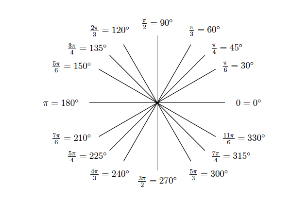
( picture taken from Precalculus’ textbook by Tradler and Carley )

( on the coordinate plane several angles are labeled indicating their measures in degrees and radians:

$$0=0^\circ, \dfrac{\pi}{6}=30^\circ, \dfrac{\pi}{4}=45^\circ, \dfrac{\pi}{3}=60^\circ,$$

$$ \dfrac{\pi}{2}=90^\circ, \dfrac{2\pi}{3}=120^\circ, \dfrac{3\pi}{4}=135^\circ, \dfrac{5\pi}{6}=150^\circ, \pi=180^\circ, $$

$$\dfrac{7\pi}{6}=210^\circ, \dfrac{5\pi}{4}=225^\circ, \dfrac{4\pi}{3}=240^\circ, $$

$$\dfrac{3\pi}{2}=270^\circ, \dfrac{5\pi}{3}=300^\circ, \dfrac{7\pi}{4}=315^\circ,\dfrac{11\pi}{6}=330^\circ .)$$

$\bigstar$ Let $P(a,b)$ be a point on the terminal side of angle $x$ with $r=\sqrt{a^2+b^2}>0$.

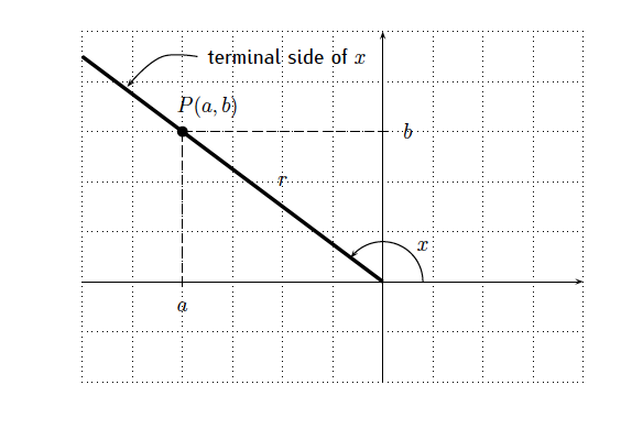
( on the coordinate plane an angle $x$ in standard position has a terminal side on QII, $P(a,b)$ is a point on the terminal side, the distance between $P(a,b)$ and the origin is $r$ .)

$$\sin x=\dfrac{b}{r}, \quad \cos x =\dfrac{a}{r}, \quad\tan x =\dfrac{b}{a}. $$

$\bigstar$ Note that

$\sin x=\dfrac{b}{r}$ is positive when $b>0$, so QI and QII

$\cos x = \dfrac{a}{r}$ is positive when $a>0$, so QI and QIV

$\tan x = \dfrac{b}{a}$ is positive when either $a,b>0$ or $a,b<0$, so QI and QIII

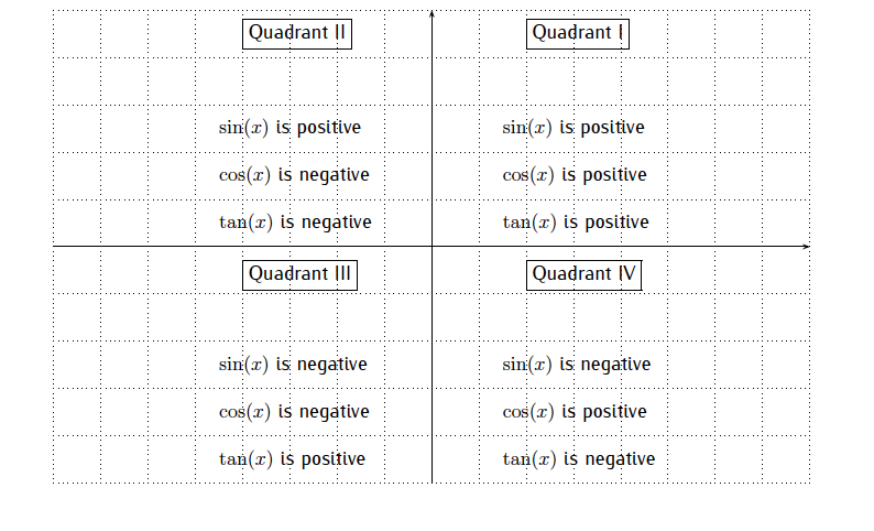
( on the coordinate plane an angle the four quadrants are marked, indicating which trig functions ( $\sin x, \cos x, \tan x$) are positive or negative in each one of them)

Video Lesson

Many times the mini-lesson will not be enough for you to start working on the problems. You need to see someone explaining the material to you. In the video you will find a variety of examples, solved step-by-step – starting from a simple one to a more complex one. Feel free to play them as many times as you need. Pause, rewind, replay, stop… follow your pace!

to be posted later

Try Questions

Now that you have read the material and watched the video, it is your turn to put in practice what you have learned. We encourage you to try the Try Questions on your own. When you are done, click on the “Show answer” tab to see if you got the correct answer.

Try Question 1

Convert $\theta = 210^{\circ}$ to radians in exact form.

$\theta = 210^{\circ}= 210\cdot\dfrac{\pi}{180} = \dfrac{210\pi}{180} = \dfrac{7\pi}{6} \text{ rad}$

Try Question 2

Find the coterminal angle with $\theta = 590^{\circ}$ whose measure is between $-180^{\circ}$ and $180^{\circ}$.

Since $-180<-130<180$, the answer is $-130^{\circ}$.

Try Question 3

 Let $\theta$ be an angle in standard position with $P(x,y) = (6,-8)$ on its terminal side. Find the six trigonometric values of $\theta$.

 If $P(x,y) = (6,-8)$, then $x=6$ and $y=-8$.  Then

\[r=\sqrt{x^2+y^2} = \sqrt{6^2+(-8)^2} = \sqrt{36+64} = \sqrt{100} = 10.\]

$$\cos\theta = \dfrac{x}{r} = \dfrac{6}{10} =\dfrac{3}{5},$$

$$\sin\theta= \dfrac{y}{r} = \dfrac{-8}{10}=-\dfrac{4}{5}, $$

$$\tan\theta= \dfrac{y}{x} = \dfrac{-8}{6}=-\dfrac{4}{3}. $$

The quadrant is II where $x<0$ and $y>0$.  We have that $y=4$, $r=5$ and

\[x = -\sqrt{r^2-y^2} = -\sqrt{25-16}=-\sqrt{9} = -3. \]

$$\cos \theta = \dfrac{x}{r} = -\dfrac{3}{5},  \qquad \tan\theta = \dfrac{y}{x} = -\dfrac{4}{3}, $$

$$\sec \theta = \dfrac{1}{\cos\theta} = -\dfrac{5}{3},  \qquad \csc\theta = \dfrac{1}{\sin\theta} = \dfrac{5}{4}, $$

$$\cot\theta = \dfrac{1}{\tan\theta} = -\dfrac{3}{4}.$$

You should now be ready to start working on the homework problems. Doing the homework is an essential part of learning. It will help you practice the lesson and reinforce your knowledge.

It is time to do the homework on WeBWork:

AngleMeasure-Radians

CoordinatePlaneTrig

When you are done, come back to this page for the Exit Questions.

Exit Questions

After doing the WeBWorK problems, come back to this page. The Exit Questions include vocabulary checking and conceptual questions. Knowing the vocabulary accurately is important for us to communicate. You will also find one last problem. All these questions will give you an idea as to whether or not you have mastered the material. Remember: the “Show Answer” tab is there for you to check your work!

• How can we divide up the unit circle and counting to find the location of $5\pi/3$ without converting to radians?  Draw a picture.  

$\bigstar$ Given $\sin\theta = \dfrac{4}{5}$ and $\cos \theta <0$, find the other five trigonometric values of $\theta$.

Show Answer

Need more help.

Don’t wait too long to do the following.

• Watch the additional video resources.
• Talk to your instructor.
• Form a study group.
• Visit a tutor. For more information, check the tutoring page .

Lessons Menu

• Lesson 1: Applications of Linear Equations
• Lesson 2: Ratio, Proportion, and Variation
• Lesson 3: The Nature of Mathematical Reasoning
• Lesson 4: Estimation and Interpreting Graphs
• Lesson 5: Problem-Solving Strategies
• Lesson 6: Statement and Quantifiers
• Lesson 7: Measures of Length: Converting Units and the Metric System
• Lesson 8: Measures of Area, Volume, and Capacity
• Lesson 9: Measures of Weight & Temperature
• Lesson 10: Percents
• Lesson 11: Simple Interest
• Lesson 12: Compound Interest
• Lesson 13: Basic Concepts of Probability
• Lesson 14: Tree Diagrams, Tables and Sample Spaces
• Lesson 15: Gathering and Organizing Data/Picturing Data
• Lesson 16: Measures of Average
• Lesson 18: Measures of Position
• Lesson 19: The Normal Distribution/Applications of the Normal Distribution
• Lesson 20: Correlation and Regression Analysis
• Lesson 21: Points, Lines, Planes & Angles
• Lesson 22: Triangles
• Lesson 23: Polygons and Perimeter/Areas of Polygons and Circles

© 2024 MAT 1190 Course Hub

Theme by Anders Noren — Up ↑

The OpenLab at City Tech: A place to learn, work, and share

The OpenLab is an open-source, digital platform designed to support teaching and learning at City Tech (New York City College of Technology), and to promote student and faculty engagement in the intellectual and social life of the college community.

New York City College of Technology | City University of New York

Accessibility

Our goal is to make the OpenLab accessible for all users.

Learn more about accessibility on the OpenLab

Creative Commons

• - Attribution
• - NonCommercial
• - ShareAlike

© New York City College of Technology | City University of New York

Chapter 9, Lesson 5: Direct Variation

• Extra Examples
• Personal Tutor
• Self-Check Quizzes

The resource you requested requires you to enter a username and password below:

Please read our Terms of Use and Privacy Notice before you explore our Web site. To report a technical problem with this Web site, please contact the site producer .

• Notifications 0

• Add Friend ($5)

As a registered member you can:

• View all solutions for free
• Request more in-depth explanations for free
• Ask our tutors any math-related question for free
• Email your homework to your parent or tutor for free
• Grade 6 McGraw Hill Glencoe - Answer Keys

Explanation:

b. Find the median and the first and third quartiles.

c. Find the interquartile range.

d. Name any outliers in the data.

For each data set, find the median, the first and third quartiles, and the interquartile range.

texts per day: 24,53,38, 12,31, 19, 26

daily attendance at the water park: 346, 250, 433,369, 422, 298

The table shows the number of minutes of exercise for each person. Compare and contrast the measures of variation for both weeks.

The table shows the number of known moons for each planet in our solar system. Use the measures of variation to describe the data.

Yes, email page to my online tutor. ( if you didn't add a tutor yet, you can add one here )

Thank you for doing your homework!

Submit Your Question

Chapter 13, Lesson 3: Measures of Variation

• Extra Examples
• Personal Tutor
• Self-Check Quizzes

The resource you requested requires you to enter a username and password below:

Please read our Terms of Use and Privacy Notice before you explore our Web site. To report a technical problem with this Web site, please contact the site producer .