assignment problem hungarian

Hungarian Method

The Hungarian method is a computational optimization technique that addresses the assignment problem in polynomial time and foreshadows following primal-dual alternatives. In 1955, Harold Kuhn used the term “Hungarian method” to honour two Hungarian mathematicians, Dénes Kőnig and Jenő Egerváry. Let’s go through the steps of the Hungarian method with the help of a solved example.

Hungarian Method to Solve Assignment Problems

The Hungarian method is a simple way to solve assignment problems. Let us first discuss the assignment problems before moving on to learning the Hungarian method.

What is an Assignment Problem?

A transportation problem is a type of assignment problem. The goal is to allocate an equal amount of resources to the same number of activities. As a result, the overall cost of allocation is minimised or the total profit is maximised.

Because available resources such as workers, machines, and other resources have varying degrees of efficiency for executing different activities, and hence the cost, profit, or loss of conducting such activities varies.

Assume we have ‘n’ jobs to do on ‘m’ machines (i.e., one job to one machine). Our goal is to assign jobs to machines for the least amount of money possible (or maximum profit). Based on the notion that each machine can accomplish each task, but at variable levels of efficiency.

Hungarian Method Steps

Check to see if the number of rows and columns are equal; if they are, the assignment problem is considered to be balanced. Then go to step 1. If it is not balanced, it should be balanced before the algorithm is applied.

Step 1 – In the given cost matrix, subtract the least cost element of each row from all the entries in that row. Make sure that each row has at least one zero.

Step 2 – In the resultant cost matrix produced in step 1, subtract the least cost element in each column from all the components in that column, ensuring that each column contains at least one zero.

Step 3 – Assign zeros

• Analyse the rows one by one until you find a row with precisely one unmarked zero. Encircle this lonely unmarked zero and assign it a task. All other zeros in the column of this circular zero should be crossed out because they will not be used in any future assignments. Continue in this manner until you’ve gone through all of the rows.
• Examine the columns one by one until you find one with precisely one unmarked zero. Encircle this single unmarked zero and cross any other zero in its row to make an assignment to it. Continue until you’ve gone through all of the columns.

Step 4 – Perform the Optimal Test

• The present assignment is optimal if each row and column has exactly one encircled zero.
• The present assignment is not optimal if at least one row or column is missing an assignment (i.e., if at least one row or column is missing one encircled zero). Continue to step 5. Subtract the least cost element from all the entries in each column of the final cost matrix created in step 1 and ensure that each column has at least one zero.

Step 5 – Draw the least number of straight lines to cover all of the zeros as follows:

(a) Highlight the rows that aren’t assigned.

(b) Label the columns with zeros in marked rows (if they haven’t already been marked).

(c) Highlight the rows that have assignments in indicated columns (if they haven’t previously been marked).

(d) Continue with (b) and (c) until no further marking is needed.

(f) Simply draw the lines through all rows and columns that are not marked. If the number of these lines equals the order of the matrix, then the solution is optimal; otherwise, it is not.

Step 6 – Find the lowest cost factor that is not covered by the straight lines. Subtract this least-cost component from all the uncovered elements and add it to all the elements that are at the intersection of these straight lines, but leave the rest of the elements alone.

Step 7 – Continue with steps 1 – 6 until you’ve found the highest suitable assignment.

Hungarian Method Example

Use the Hungarian method to solve the given assignment problem stated in the table. The entries in the matrix represent each man’s processing time in hours.

\(\begin{array}{l}\begin{bmatrix} & I & II & III & IV & V \\1 & 20 & 15 & 18 & 20 & 25 \\2 & 18 & 20 & 12 & 14 & 15 \\3 & 21 & 23 & 25 & 27 & 25 \\4 & 17 & 18 & 21 & 23 & 20 \\5 & 18 & 18 & 16 & 19 & 20 \\\end{bmatrix}\end{array} \)

With 5 jobs and 5 men, the stated problem is balanced.

\(\begin{array}{l}A = \begin{bmatrix}20 & 15 & 18 & 20 & 25 \\18 & 20 & 12 & 14 & 15 \\21 & 23 & 25 & 27 & 25 \\17 & 18 & 21 & 23 & 20 \\18 & 18 & 16 & 19 & 20 \\\end{bmatrix}\end{array} \)

Subtract the lowest cost element in each row from all of the elements in the given cost matrix’s row. Make sure that each row has at least one zero.

\(\begin{array}{l}A = \begin{bmatrix}5 & 0 & 3 & 5 & 10 \\6 & 8 & 0 & 2 & 3 \\0 & 2 & 4 & 6 & 4 \\0 & 1 & 4 & 6 & 3 \\2 & 2 & 0 & 3 & 4 \\\end{bmatrix}\end{array} \)

Subtract the least cost element in each Column from all of the components in the given cost matrix’s Column. Check to see if each column has at least one zero.

\(\begin{array}{l}A = \begin{bmatrix}5 & 0 & 3 & 3 & 7 \\6 & 8 & 0 & 0 & 0 \\0 & 2 & 4 & 4 & 1 \\0 & 1 & 4 & 4 & 0 \\2 & 2 & 0 & 1 & 1 \\\end{bmatrix}\end{array} \)

When the zeros are assigned, we get the following:

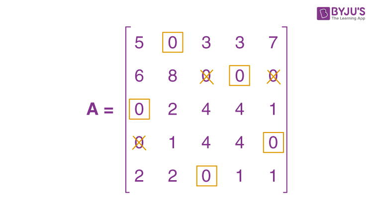
The present assignment is optimal because each row and column contain precisely one encircled zero.

Where 1 to II, 2 to IV, 3 to I, 4 to V, and 5 to III are the best assignments.

Hence, z = 15 + 14 + 21 + 20 + 16 = 86 hours is the optimal time.

Practice Question on Hungarian Method

Use the Hungarian method to solve the following assignment problem shown in table. The matrix entries represent the time it takes for each job to be processed by each machine in hours.

\(\begin{array}{l}\begin{bmatrix}J/M & I & II & III & IV & V \\1 & 9 & 22 & 58 & 11 & 19 \\2 & 43 & 78 & 72 & 50 & 63 \\3 & 41 & 28 & 91 & 37 & 45 \\4 & 74 & 42 & 27 & 49 & 39 \\5 & 36 & 11 & 57 & 22 & 25 \\\end{bmatrix}\end{array} \)

Stay tuned to BYJU’S – The Learning App and download the app to explore all Maths-related topics.

Frequently Asked Questions on Hungarian Method

What is hungarian method.

The Hungarian method is defined as a combinatorial optimization technique that solves the assignment problems in polynomial time and foreshadowed subsequent primal–dual approaches.

What are the steps involved in Hungarian method?

The following is a quick overview of the Hungarian method: Step 1: Subtract the row minima. Step 2: Subtract the column minimums. Step 3: Use a limited number of lines to cover all zeros. Step 4: Add some more zeros to the equation.

What is the purpose of the Hungarian method?

When workers are assigned to certain activities based on cost, the Hungarian method is beneficial for identifying minimum costs.

Leave a Comment Cancel reply

Your Mobile number and Email id will not be published. Required fields are marked *

Request OTP on Voice Call

Post My Comment

• Share Share

Register with BYJU'S & Download Free PDFs

Register with byju's & watch live videos.

Reset password New user? Sign up

Existing user? Log in

Hungarian Maximum Matching Algorithm

Already have an account? Log in here.

The Hungarian matching algorithm , also called the Kuhn-Munkres algorithm, is a \(O\big(|V|^3\big)\) algorithm that can be used to find maximum-weight matchings in bipartite graphs , which is sometimes called the assignment problem . A bipartite graph can easily be represented by an adjacency matrix , where the weights of edges are the entries. Thinking about the graph in terms of an adjacency matrix is useful for the Hungarian algorithm.

A matching corresponds to a choice of 1s in the adjacency matrix, with at most one 1 in each row and in each column.

The Hungarian algorithm solves the following problem:

In a complete bipartite graph \(G\), find the maximum-weight matching. (Recall that a maximum-weight matching is also a perfect matching.)

This can also be adapted to find the minimum-weight matching.

Say you are having a party and you want a musician to perform, a chef to prepare food, and a cleaning service to help clean up after the party. There are three companies that provide each of these three services, but one company can only provide one service at a time (i.e. Company B cannot provide both the cleaners and the chef). You are deciding which company you should purchase each service from in order to minimize the cost of the party. You realize that is an example of the assignment problem, and set out to make a graph out of the following information: \(\quad\) Company\(\quad\) \(\quad\) Cost for Musician\(\quad\) \(\quad\) Cost for Chef\(\quad\) \(\quad\) Cost for Cleaners\(\quad\) \(\quad\) Company A\(\quad\) \(\quad\) $108\(\quad\) \(\quad\) $125\(\quad\) \(\quad\) $150\(\quad\) \(\quad\) Company B\(\quad\) \(\quad\) $150\(\quad\) \(\quad\) $135\(\quad\) \(\quad\) $175\(\quad\) \(\quad\) Company C\(\quad\) \(\quad\) $122\(\quad\) \(\quad\) $148\(\quad\) \(\quad\) $250\(\quad\) Can you model this table as a graph? What are the nodes? What are the edges? Show Answer The nodes are the companies and the services. The edges are weighted by the price.

What are some ways to solve the problem above? Since the table above can be thought of as a \(3 \times 3\) matrix, one could certainly solve this problem using brute force, checking every combination and seeing what yields the lowest price. However, there are \(n!\) combinations to check, and for large \(n\), this method becomes very inefficient very quickly.

The Hungarian Algorithm Using an Adjacency Matrix

The hungarian algorithm using a graph.

With the cost matrix from the example above in mind, the Hungarian algorithm operates on this key idea: if a number is added to or subtracted from all of the entries of any one row or column of a cost matrix, then an optimal assignment for the resulting cost matrix is also an optimal assignment for the original cost matrix.

The Hungarian Method [1] Subtract the smallest entry in each row from all the other entries in the row. This will make the smallest entry in the row now equal to 0. Subtract the smallest entry in each column from all the other entries in the column. This will make the smallest entry in the column now equal to 0. Draw lines through the row and columns that have the 0 entries such that the fewest lines possible are drawn. If there are \(n\) lines drawn, an optimal assignment of zeros is possible and the algorithm is finished. If the number of lines is less than \(n\), then the optimal number of zeroes is not yet reached. Go to the next step. Find the smallest entry not covered by any line. Subtract this entry from each row that isn’t crossed out, and then add it to each column that is crossed out. Then, go back to Step 3.

Solve for the optimal solution for the example in the introduction using the Hungarian algorithm described above. Here is the initial adjacency matrix: Subtract the smallest value in each row from the other values in the row: Now, subtract the smallest value in each column from all other values in the column: Draw lines through the row and columns that have the 0 entries such that the fewest possible lines are drawn: There are 2 lines drawn, and 2 is less than 3, so there is not yet the optimal number of zeroes. Find the smallest entry not covered by any line. Subtract this entry from each row that isn’t crossed out, and then add it to each column that is crossed out. Then, go back to Step 3. 2 is the smallest entry. First, subtract from the uncovered rows: Now add to the covered columns: Now go back to step 3, drawing lines through the rows and columns that have 0 entries: There are 3 lines (which is \(n\)), so we are done. The assignment will be where the 0's are in the matrix such that only one 0 per row and column is part of the assignment. Replace the original values: The Hungarian algorithm tells us that it is cheapest to go with the musician from company C, the chef from company B, and the cleaners from company A. We can verify this by brute force. 108 + 135 + 250 = 493 108 + 148 + 175 = 431 150 + 125 + 250 = 525 150 + 148 + 150 = 448 122 + 125 + 175 = 422 122 + 135 + 150 = 407. We can see that 407 is the lowest price and matches the assignment the Hungarian algorithm determined. \(_\square\)

The Hungarian algorithm can also be executed by manipulating the weights of the bipartite graph in order to find a stable, maximum (or minimum) weight matching. This can be done by finding a feasible labeling of a graph that is perfectly matched, where a perfect matching is denoted as every vertex having exactly one edge of the matching.

How do we know that this creates a maximum-weight matching?

A feasible labeling on a perfect match returns a maximum-weighted matching. Suppose each edge \(e\) in the graph \(G\) connects two vertices, and every vertex \(v\) is covered exactly once. With this, we have the following inequality: \[w(M’) = \sum_{e\ \epsilon\ E} w(e) \leq \sum_{e\ \epsilon\ E } \big(l(e_x) + l(e_y)\big) = \sum_{v\ \epsilon\ V} l(v),\] where \(M’\) is any perfect matching in \(G\) created by a random assignment of vertices, and \(l(x)\) is a numeric label to node \(x\). This means that \(\sum_{v\ \epsilon\ V}\ l(v)\) is an upper bound on the cost of any perfect matching. Now let \(M\) be a perfect match in \(G\), then \[w(M) = \sum_{e\ \epsilon\ E} w(e) = \sum_{v\ \epsilon\ V}\ l(v).\] So \(w(M’) \leq w(M)\) and \(M\) is optimal. \(_\square\)

Start the algorithm by assigning any weight to each individual node in order to form a feasible labeling of the graph \(G\). This labeling will be improved upon by finding augmenting paths for the assignment until the optimal one is found.

A feasible labeling is a labeling such that

\(l(x) + l(y) \geq w(x,y)\ \forall x \in X, y \in Y\), where \(X\) is the set of nodes on one side of the bipartite graph, \(Y\) is the other set of nodes, \(l(x)\) is the label of \(x\), etc., and \(w(x,y)\) is the weight of the edge between \(x\) and \(y\).

A simple feasible labeling is just to label a node with the number of the largest weight from an edge going into the node. This is certain to be a feasible labeling because if \(A\) is a node connected to \(B\), the label of \(A\) plus the label of \(B\) is greater than or equal to the weight \(w(x,y)\) for all \(y\) and \(x\).

A feasible labeling of nodes, where labels are in red [2] .

Imagine there are four soccer players and each can play a few positions in the field. The team manager has quantified their skill level playing each position to make assignments easier.

How can players be assigned to positions in order to maximize the amount of skill points they provide?

The algorithm starts by labeling all nodes on one side of the graph with the maximum weight. This can be done by finding the maximum-weighted edge and labeling the adjacent node with it. Additionally, match the graph with those edges. If a node has two maximum edges, don’t connect them.

Although Eva is the best suited to play defense, she can't play defense and mid at the same time!

If the matching is perfect, the algorithm is done as there is a perfect matching of maximum weights. Otherwise, there will be two nodes that are not connected to any other node, like Tom and Defense. If this is the case, begin iterating.

Improve the labeling by finding the non-zero label vertex without a match, and try to find the best assignment for it. Formally, the Hungarian matching algorithm can be executed as defined below:

The Hungarian Algorithm for Graphs [3] Given: the labeling \(l\), an equality graph \(G_l = (V, E_l)\), an initial matching \(M\) in \(G_l\), and an unmatched vertex \(u \in V\) and \(u \notin M\) Augmenting the matching A path is augmenting for \(M\) in \(G_l\) if it alternates between edges in the matching and edges not in the matching, and the first and last vertices are free vertices , or unmatched, in \(M\). We will keep track of a candidate augmenting path starting at the vertex \(u\). If the algorithm finds an unmatched vertex \(v\), add on to the existing augmenting path \(p\) by adding the \(u\) to \(v\) segment. Flip the matching by replacing the edges in \(M\) with the edges in the augmenting path that are not in \(M\) \((\)in other words, the edges in \(E_l - M).\) Improving the labeling \(S \subseteq X\) and \(T \subseteq Y,\) where \(S\) and \(T\) represent the candidate augmenting alternating path between the matching and the edges not in the matching. Let \(N_l(S)\) be the neighbors to each node that is in \(S\) along edges in \(E_l\) such that \(N_l(S) = \{v|\forall u \in S: (u,v) \in E_l\}\). If \(N_l(S) = T\), then we cannot increase the size of the alternating path (and therefore can't further augment), so we need to improve the labeling. Let \(\delta_l\) be the minimum of \(l(u) + l(v) - w(u,v)\) over all of the \(u \in S\) and \(v \notin T\). Improve the labeling \(l\) to \(l'\): If \(r \in S,\) then \(l'(r) = l(r) - \delta_l,\) If \(r \in T,\) then \(l'(r) = l(r) + \delta_l.\) If \(r \notin S\) and \(r \notin T,\) then \(l'(r) = l(r).\) \(l'\) is a valid labeling and \(E_l \subset E_{l'}.\) Putting it all together: The Hungarian Algorithm Start with some matching \(M\), a valid labeling \(l\), where \(l\) is defined as the labelling \(\forall x \in X, y \in Y| l(y) = 0, l(x) = \text{ max}_{y \in Y}(w\big(x, y)\big)\). Do these steps until a perfect matching is found \((\)when \(M\) is perfect\():\) (a) Look for an augmenting path in \(M.\) (b) If an augmenting path does not exist, improve the labeling and then go back to step (a).

Each step will increase the size of the matching \(M\) or it will increase the size of the set of labeled edges, \(E_l\). This means that the process will eventually terminate since there are only so many edges in the graph \(G\). [4]

When the process terminates, \(M\) will be a perfect matching. By the Kuhn-Munkres theorem , this means that the matching is a maximum-weight matching.

The algorithm defined above can be implemented in the soccer scenario. First, the conflicting node is identified, implying that there is an alternating tree that must be reconfigured.

There is an alternating path between defense, Eva, mid, and Tom.

To find the best appropriate node, find the minimum \(\delta_l\), as defined in step 4 above, where \(l_u\) is the label for player \(u,\) \(l_v\) is the label for position \(v,\) and \(w_{u, v}\) is the weight on that edge.

The \(\delta_l\) of each unmatched node is computed, where the minimum is found to be a value of 2, between Tom playing mid \((8 + 0 – 6 = 2).\)

The labels are then augmented and the new edges are graphed in the example. Notice that defense and mid went down by 2 points, whereas Eva’s skillset got back two points. However, this is expected as Eva can't play in both positions at once.

Augmenting path leads to relabeling of nodes, which gives rise to the maximum-weighted path.

These new edges complete the perfect matching of the graph, which implies that a maximum-weighted graph has been found and the algorithm can terminate.

The complexity of the algorithm will be analyzed using the graph-based technique as a reference, yet the result is the same as for the matrix-based one.

Algorithm analysis [3] At each \(a\) or \(b\) step, the algorithm adds one edge to the matching and this happens \(O\big(|V|\big)\) times. It takes \(O\big(|V|\big)\) time to find the right vertex for the augmenting (if there is one at all), and it is \(O\big(|V|\big)\) time to flip the matching. Improving the labeling takes \(O\big(|V|\big)\) time to find \(\delta_l\) and to update the labelling accordingly. We might have to improve the labeling up to \(O\big(|V|\big)\) times if there is no augmenting path. This makes for a total of \(O\big(|V|^2\big)\) time. In all, there are \(O\big(|V|\big)\) iterations each taking \(O\big(|V|\big)\) work, leading to a total running time of \(O\big(|V|^3\big)\).

• Matching Algorithms
• Bruff, D. The Assignment Problem and the Hungarian Method . Retrieved June 26, 2016, from http://www.math.harvard.edu/archive/20_spring_05/handouts/assignment_overheads.pdf
• Golin, M. Bipartite Matching & the Hungarian Method . Retrieved Retrieved June 26th, 2016, from http://www.cse.ust.hk/~golin/COMP572/Notes/Matching.pdf
• Grinman, A. The Hungarian Algorithm for Weighted Bipartite Graphs . Retrieved June 26, 2016, from http://math.mit.edu/~rpeng/18434/hungarianAlgorithm.pdf
• Golin, M. Bipartite Matching & the Hungarian Method . Retrieved June 26, 2016, from http://www.cse.ust.hk/~golin/COMP572/Notes/Matching.pdf

Problem Loading...

Note Loading...

Set Loading...

• Data Structures
• Linked List
• Binary Tree
• Binary Search Tree
• Segment Tree
• Disjoint Set Union
• Fenwick Tree
• Red-Black Tree
• Advanced Data Structures

Hungarian Algorithm for Assignment Problem | Set 2 (Implementation)

• Hungarian Algorithm for Assignment Problem | Set 1 (Introduction)
• Implementation of Exhaustive Search Algorithm for Set Packing
• Greedy Approximate Algorithm for Set Cover Problem
• Introduction to Exact Cover Problem and Algorithm X
• Job Assignment Problem using Branch And Bound
• Prim's Algorithm (Simple Implementation for Adjacency Matrix Representation)
• Introduction to Disjoint Set (Union-Find Algorithm)
• Channel Assignment Problem
• Java Program for Counting sets of 1s and 0s in a binary matrix
• Top 20 Greedy Algorithms Interview Questions
• C++ Program for Counting sets of 1s and 0s in a binary matrix
• C# Program for Dijkstra's shortest path algorithm | Greedy Algo-7
• Java Program for Dijkstra's shortest path algorithm | Greedy Algo-7
• C / C++ Program for Dijkstra's shortest path algorithm | Greedy Algo-7
• Self assignment check in assignment operator
• Python Program for Dijkstra's shortest path algorithm | Greedy Algo-7
• Algorithms | Dynamic Programming | Question 7
• Assignment Operators in C
• Assignment Operators in Programming
• Merge Sort - Data Structure and Algorithms Tutorials
• Must Do Coding Questions for Companies like Amazon, Microsoft, Adobe, ...
• QuickSort - Data Structure and Algorithm Tutorials
• Bubble Sort - Data Structure and Algorithm Tutorials
• Tree Traversal Techniques - Data Structure and Algorithm Tutorials
• Binary Search - Data Structure and Algorithm Tutorials
• Insertion Sort - Data Structure and Algorithm Tutorials
• Selection Sort – Data Structure and Algorithm Tutorials
• Understanding the basics of Linked List
• Breadth First Search or BFS for a Graph

Given a 2D array , arr of size N*N where arr[i][j] denotes the cost to complete the j th job by the i th worker. Any worker can be assigned to perform any job. The task is to assign the jobs such that exactly one worker can perform exactly one job in such a way that the total cost of the assignment is minimized.

Input: arr[][] = {{3, 5}, {10, 1}} Output: 4 Explanation: The optimal assignment is to assign job 1 to the 1st worker, job 2 to the 2nd worker. Hence, the optimal cost is 3 + 1 = 4. Input: arr[][] = {{2500, 4000, 3500}, {4000, 6000, 3500}, {2000, 4000, 2500}} Output: 4 Explanation: The optimal assignment is to assign job 2 to the 1st worker, job 3 to the 2nd worker and job 1 to the 3rd worker. Hence, the optimal cost is 4000 + 3500 + 2000 = 9500.

Different approaches to solve this problem are discussed in this article .

Approach: The idea is to use the Hungarian Algorithm to solve this problem. The algorithm is as follows:

• For each row of the matrix, find the smallest element and subtract it from every element in its row.
• Repeat the step 1 for all columns.
• Cover all zeros in the matrix using the minimum number of horizontal and vertical lines.
• Test for Optimality : If the minimum number of covering lines is N , an optimal assignment is possible. Else if lines are lesser than N , an optimal assignment is not found and must proceed to step 5.
• Determine the smallest entry not covered by any line. Subtract this entry from each uncovered row, and then add it to each covered column. Return to step 3.

Consider an example to understand the approach:

Let the 2D array be: 2500 4000 3500 4000 6000 3500 2000 4000 2500 Step 1: Subtract minimum of every row. 2500, 3500 and 2000 are subtracted from rows 1, 2 and 3 respectively. 0   1500  1000 500  2500   0 0   2000  500 Step 2: Subtract minimum of every column. 0, 1500 and 0 are subtracted from columns 1, 2 and 3 respectively. 0    0   1000 500  1000   0 0   500  500 Step 3: Cover all zeroes with minimum number of horizontal and vertical lines. Step 4: Since we need 3 lines to cover all zeroes, the optimal assignment is found.   2500   4000  3500  4000  6000   3500   2000  4000  2500 So the optimal cost is 4000 + 3500 + 2000 = 9500

For implementing the above algorithm, the idea is to use the max_cost_assignment() function defined in the dlib library . This function is an implementation of the Hungarian algorithm (also known as the Kuhn-Munkres algorithm) which runs in O(N 3 ) time. It solves the optimal assignment problem. 

Below is the implementation of the above approach:

Time Complexity: O(N 3 ) Auxiliary Space: O(N 2 )

Please Login to comment...

Similar reads.

• Mathematical

Improve your Coding Skills with Practice

What kind of Experience do you want to share?

Index     Assignment problem     Hungarian algorithm     Solve online    

The Hungarian algorithm: An example

We consider an example where four jobs (J1, J2, J3, and J4) need to be executed by four workers (W1, W2, W3, and W4), one job per worker. The matrix below shows the cost of assigning a certain worker to a certain job. The objective is to minimize the total cost of the assignment.

Below we will explain the Hungarian algorithm using this example. Note that a general description of the algorithm can be found here .

Step 1: Subtract row minima

We start with subtracting the row minimum from each row. The smallest element in the first row is, for example, 69. Therefore, we substract 69 from each element in the first row. The resulting matrix is:

Step 2: Subtract column minima

Similarly, we subtract the column minimum from each column, giving the following matrix:

Step 3: Cover all zeros with a minimum number of lines

We will now determine the minimum number of lines (horizontal or vertical) that are required to cover all zeros in the matrix. All zeros can be covered using 3 lines:

Step 4: Create additional zeros

First, we find that the smallest uncovered number is 6. We subtract this number from all uncovered elements and add it to all elements that are covered twice. This results in the following matrix:

Now we return to Step 3.

Again, We determine the minimum number of lines required to cover all zeros in the matrix. Now there are 4 lines required:

Because the number of lines required (4) equals the size of the matrix ( n =4), an optimal assignment exists among the zeros in the matrix. Therefore, the algorithm stops.

The optimal assignment

The following zeros cover an optimal assignment:

This corresponds to the following optimal assignment in the original cost matrix:

Thus, worker 1 should perform job 3, worker 2 job 2, worker 3 job 1, and worker 4 should perform job 4. The total cost of this optimal assignment is to 69 + 37 + 11 + 23 = 140.

Solve your own problem online

HungarianAlgorithm.com © 2013-2024

The Hungarian Method for the Assignment Problem

• First Online: 01 January 2009

Cite this chapter

• Harold W. Kuhn 9  

9620 Accesses

185 Citations

11 Altmetric

This paper has always been one of my favorite “children,” combining as it does elements of the duality of linear programming and combinatorial tools from graph theory. It may be of some interest to tell the story of its origin.

This is a preview of subscription content, log in via an institution to check access.

Access this chapter

• Available as PDF
• Read on any device
• Instant download
• Own it forever

Tax calculation will be finalised at checkout

Purchases are for personal use only

Institutional subscriptions

Unable to display preview.  Download preview PDF.

H.W. Kuhn, On the origin of the Hungarian Method , History of mathematical programming; a collection of personal reminiscences (J.K. Lenstra, A.H.G. Rinnooy Kan, and A. Schrijver, eds.), North Holland, Amsterdam, 1991, pp. 77–81.

Google Scholar  

A. Schrijver, Combinatorial optimization: polyhedra and efficiency , Vol. A. Paths, Flows, Matchings, Springer, Berlin, 2003.

MATH   Google Scholar  

Download references

Author information

Authors and affiliations.

Princeton University, Princeton, USA

Harold W. Kuhn

You can also search for this author in PubMed   Google Scholar

Corresponding author

Correspondence to Harold W. Kuhn .

Editor information

Editors and affiliations.

Inst. Informatik, Universität Köln, Pohligstr. 1, Köln, 50969, Germany

Michael Jünger

Fac. Sciences de Base (FSB), Ecole Polytechnique Fédérale de Lausanne, Lausanne, 1015, Switzerland

Thomas M. Liebling

Ensimag, Institut Polytechnique de Grenoble, avenue Félix Viallet 46, Grenoble CX 1, 38031, France

Denis Naddef

School of Industrial &, Georgia Institute of Technology, Ferst Drive NW., 765, Atlanta, 30332-0205, USA

George L. Nemhauser

IBM Corporation, Route 100 294, Somers, 10589, USA

William R. Pulleyblank

Inst. Informatik, Universität Heidelberg, Im Neuenheimer Feld 326, Heidelberg, 69120, Germany

Gerhard Reinelt

ed Informatica, CNR - Ist. Analisi dei Sistemi, Viale Manzoni 30, Roma, 00185, Italy

Giovanni Rinaldi

Center for Operations Reserach &, Université Catholique de Louvain, voie du Roman Pays 34, Leuven, 1348, Belgium

Laurence A. Wolsey

Rights and permissions

Reprints and permissions

Copyright information

© 2010 Springer-Verlag Berlin Heidelberg

About this chapter

Kuhn, H.W. (2010). The Hungarian Method for the Assignment Problem. In: Jünger, M., et al. 50 Years of Integer Programming 1958-2008. Springer, Berlin, Heidelberg. https://doi.org/10.1007/978-3-540-68279-0_2

Download citation

DOI : https://doi.org/10.1007/978-3-540-68279-0_2

Published : 06 November 2009

Publisher Name : Springer, Berlin, Heidelberg

Print ISBN : 978-3-540-68274-5

Online ISBN : 978-3-540-68279-0

eBook Packages : Mathematics and Statistics Mathematics and Statistics (R0)

Share this chapter

Anyone you share the following link with will be able to read this content:

Sorry, a shareable link is not currently available for this article.

Provided by the Springer Nature SharedIt content-sharing initiative

• Publish with us

Policies and ethics

• Find a journal
• Track your research

Hungarian Method Examples

Now we will examine a few highly simplified illustrations of Hungarian Method for solving an assignment problem .

Later in the chapter, you will find more practical versions of assignment models like Crew assignment problem , Travelling salesman problem , etc.

Example-1, Example-2

Example 1: Hungarian Method

The Funny Toys Company has four men available for work on four separate jobs. Only one man can work on any one job. The cost of assigning each man to each job is given in the following table. The objective is to assign men to jobs in such a way that the total cost of assignment is minimum.

This is a minimization example of assignment problem . We will use the Hungarian Algorithm to solve this problem.

Identify the minimum element in each row and subtract it from every element of that row. The result is shown in the following table.

"A man has one hundred dollars and you leave him with two dollars, that's subtraction." -Mae West

On small screens, scroll horizontally to view full calculation

Identify the minimum element in each column and subtract it from every element of that column.

Make the assignments for the reduced matrix obtained from steps 1 and 2 in the following way:

• For every zero that becomes assigned, cross out (X) all other zeros in the same row and the same column.
• If for a row and a column, there are two or more zeros and one cannot be chosen by inspection, choose the cell arbitrarily for assignment.

An optimal assignment is found, if the number of assigned cells equals the number of rows (and columns). In case you have chosen a zero cell arbitrarily, there may be alternate optimal solutions. If no optimal solution is found, go to step 5.

Use Horizontal Scrollbar to View Full Table Calculation

Draw the minimum number of vertical and horizontal lines necessary to cover all the zeros in the reduced matrix obtained from step 3 by adopting the following procedure:

• Mark all the rows that do not have assignments.
• Mark all the columns (not already marked) which have zeros in the marked rows.
• Mark all the rows (not already marked) that have assignments in marked columns.
• Repeat steps 5 (ii) and (iii) until no more rows or columns can be marked.
• Draw straight lines through all unmarked rows and marked columns.

You can also draw the minimum number of lines by inspection.

Select the smallest element (i.e., 1) from all the uncovered elements. Subtract this smallest element from all the uncovered elements and add it to the elements, which lie at the intersection of two lines. Thus, we obtain another reduced matrix for fresh assignment.

Now again make the assignments for the reduced matrix.

Final Table: Hungarian Method

Since the number of assignments is equal to the number of rows (& columns), this is the optimal solution.

The total cost of assignment = A1 + B4 + C2 + D3

Substituting values from original table: 20 + 17 + 17 + 24 = Rs. 78.

Share This Article

Operations Research Simplified Back Next

Goal programming Linear programming Simplex Method Transportation Problem

• Implementation of the Hungarian algorithm
• Connection to the Successive Shortest Path Algorithm
• Task examples
• Practice Problems

Hungarian algorithm for solving the assignment problem ¶

Statement of the assignment problem ¶.

There are several standard formulations of the assignment problem (all of which are essentially equivalent). Here are some of them:

There are $n$ jobs and $n$ workers. Each worker specifies the amount of money they expect for a particular job. Each worker can be assigned to only one job. The objective is to assign jobs to workers in a way that minimizes the total cost.

Given an $n \times n$ matrix $A$ , the task is to select one number from each row such that exactly one number is chosen from each column, and the sum of the selected numbers is minimized.

Given an $n \times n$ matrix $A$ , the task is to find a permutation $p$ of length $n$ such that the value $\sum A[i]\left[p[i]\right]$ is minimized.

Consider a complete bipartite graph with $n$ vertices per part, where each edge is assigned a weight. The objective is to find a perfect matching with the minimum total weight.

It is important to note that all the above scenarios are " square " problems, meaning both dimensions are always equal to $n$ . In practice, similar " rectangular " formulations are often encountered, where $n$ is not equal to $m$ , and the task is to select $\min(n,m)$ elements. However, it can be observed that a "rectangular" problem can always be transformed into a "square" problem by adding rows or columns with zero or infinite values, respectively.

We also note that by analogy with the search for a minimum solution, one can also pose the problem of finding a maximum solution. However, these two problems are equivalent to each other: it is enough to multiply all the weights by $-1$ .

Hungarian algorithm ¶

Historical reference ¶.

The algorithm was developed and published by Harold Kuhn in 1955. Kuhn himself gave it the name "Hungarian" because it was based on the earlier work by Hungarian mathematicians Dénes Kőnig and Jenő Egerváry. In 1957, James Munkres showed that this algorithm runs in (strictly) polynomial time, independently from the cost. Therefore, in literature, this algorithm is known not only as the "Hungarian", but also as the "Kuhn-Mankres algorithm" or "Mankres algorithm". However, it was recently discovered in 2006 that the same algorithm was invented a century before Kuhn by the German mathematician Carl Gustav Jacobi . His work, About the research of the order of a system of arbitrary ordinary differential equations , which was published posthumously in 1890, contained, among other findings, a polynomial algorithm for solving the assignment problem. Unfortunately, since the publication was in Latin, it went unnoticed among mathematicians.

It is also worth noting that Kuhn's original algorithm had an asymptotic complexity of $\mathcal{O}(n^4)$ , and only later Jack Edmonds and Richard Karp (and independently Tomizawa ) showed how to improve it to an asymptotic complexity of $\mathcal{O}(n^3)$ .

The $\mathcal{O}(n^4)$ algorithm ¶

To avoid ambiguity, we note right away that we are mainly concerned with the assignment problem in a matrix formulation (i.e., given a matrix $A$ , you need to select $n$ cells from it that are in different rows and columns). We index arrays starting with $1$ , i.e., for example, a matrix $A$ has indices $A[1 \dots n][1 \dots n]$ .

We will also assume that all numbers in matrix A are non-negative (if this is not the case, you can always make the matrix non-negative by adding some constant to all numbers).

Let's call a potential two arbitrary arrays of numbers $u[1 \ldots n]$ and $v[1 \ldots n]$ , such that the following condition is satisfied:

(As you can see, $u[i]$ corresponds to the $i$ -th row, and $v[j]$ corresponds to the $j$ -th column of the matrix).

Let's call the value $f$ of the potential the sum of its elements:

On one hand, it is easy to see that the cost of the desired solution $sol$ is not less than the value of any potential.

Lemma. $sol\geq f.$

The desired solution of the problem consists of $n$ cells of the matrix $A$ , so $u[i]+v[j]\leq A[i][j]$ for each of them. Since all the elements in $sol$ are in different rows and columns, summing these inequalities over all the selected $A[i][j]$ , you get $f$ on the left side of the inequality, and $sol$ on the right side.

On the other hand, it turns out that there is always a solution and a potential that turns this inequality into equality . The Hungarian algorithm described below will be a constructive proof of this fact. For now, let's just pay attention to the fact that if any solution has a cost equal to any potential, then this solution is optimal .

Let's fix some potential. Let's call an edge $(i,j)$ rigid if $u[i]+v[j]=A[i][j].$

Recall an alternative formulation of the assignment problem, using a bipartite graph. Denote with $H$ a bipartite graph composed only of rigid edges. The Hungarian algorithm will maintain, for the current potential, the maximum-number-of-edges matching $M$ of the graph $H$ . As soon as $M$ contains $n$ edges, then the solution to the problem will be just $M$ (after all, it will be a solution whose cost coincides with the value of a potential).

Let's proceed directly to the description of the algorithm .

Step 1. At the beginning, the potential is assumed to be zero ( $u[i]=v[i]=0$ for all $i$ ), and the matching $M$ is assumed to be empty.

Step 2. Further, at each step of the algorithm, we try, without changing the potential, to increase the cardinality of the current matching $M$ by one (recall that the matching is searched in the graph of rigid edges $H$ ). To do this, the usual Kuhn Algorithm for finding the maximum matching in bipartite graphs is used. Let us recall the algorithm here. All edges of the matching $M$ are oriented in the direction from the right part to the left one, and all other edges of the graph $H$ are oriented in the opposite direction.

Recall (from the terminology of searching for matchings) that a vertex is called saturated if an edge of the current matching is adjacent to it. A vertex that is not adjacent to any edge of the current matching is called unsaturated. A path of odd length, in which the first edge does not belong to the matching, and for all subsequent edges there is an alternating belonging to the matching (belongs/does not belong) - is called an augmenting path. From all unsaturated vertices in the left part, a depth-first or breadth-first traversal is started. If, as a result of the search, it was possible to reach an unsaturated vertex of the right part, we have found an augmenting path from the left part to the right one. If we include odd edges of the path and remove the even ones in the matching (i.e. include the first edge in the matching, exclude the second, include the third, etc.), then we will increase the matching cardinality by one.

If there was no augmenting path, then the current matching $M$ is maximal in the graph $H$ .

Step 3. If at the current step, it is not possible to increase the cardinality of the current matching, then a recalculation of the potential is performed in such a way that, at the next steps, there will be more opportunities to increase the matching.

Denote by $Z_1$ the set of vertices of the left part that were visited during the last traversal of Kuhn's algorithm, and through $Z_2$ the set of visited vertices of the right part.

Let's calculate the value $\Delta$ :

Lemma. $\Delta > 0.$

Suppose $\Delta=0$ . Then there exists a rigid edge $(i,j)$ with $i\in Z_1$ and $j\notin Z_2$ . It follows that the edge $(i,j)$ must be oriented from the right part to the left one, i.e. $(i,j)$ must be included in the matching $M$ . However, this is impossible, because we could not get to the saturated vertex $i$ except by going along the edge from j to i. So $\Delta > 0$ .

Now let's recalculate the potential in this way:

for all vertices $i\in Z_1$ , do $u[i] \gets u[i]+\Delta$ ,

for all vertices $j\in Z_2$ , do $v[j] \gets v[j]-\Delta$ .

Lemma. The resulting potential is still a correct potential.

We will show that, after recalculation, $u[i]+v[j]\leq A[i][j]$ for all $i,j$ . For all the elements of $A$ with $i\in Z_1$ and $j\in Z_2$ , the sum $u[i]+v[j]$ does not change, so the inequality remains true. For all the elements with $i\notin Z_1$ and $j\in Z_2$ , the sum $u[i]+v[j]$ decreases by $\Delta$ , so the inequality is still true. For the other elements whose $i\in Z_1$ and $j\notin Z_2$ , the sum increases, but the inequality is still preserved, since the value $\Delta$ is, by definition, the maximum increase that does not change the inequality.

Lemma. The old matching $M$ of rigid edges is valid, i.e. all edges of the matching will remain rigid.

For some rigid edge $(i,j)$ to stop being rigid as a result of a change in potential, it is necessary that equality $u[i] + v[j] = A[i][j]$ turns into inequality $u[i] + v[j] < A[i][j]$ . However, this can happen only when $i \notin Z_1$ and $j \in Z_2$ . But $i \notin Z_1$ implies that the edge $(i,j)$ could not be a matching edge.

Lemma. After each recalculation of the potential, the number of vertices reachable by the traversal, i.e. $|Z_1|+|Z_2|$ , strictly increases.

First, note that any vertex that was reachable before recalculation, is still reachable. Indeed, if some vertex is reachable, then there is some path from reachable vertices to it, starting from the unsaturated vertex of the left part; since for edges of the form $(i,j),\ i\in Z_1,\ j\in Z_2$ the sum $u[i]+v[j]$ does not change, this entire path will be preserved after changing the potential. Secondly, we show that after a recalculation, at least one new vertex will be reachable. This follows from the definition of $\Delta$ : the edge $(i,j)$ which $\Delta$ refers to will become rigid, so vertex $j$ will be reachable from vertex $i$ .

Due to the last lemma, no more than $n$ potential recalculations can occur before an augmenting path is found and the matching cardinality of $M$ is increased. Thus, sooner or later, a potential that corresponds to a perfect matching $M^*$ will be found, and $M^*$ will be the answer to the problem. If we talk about the complexity of the algorithm, then it is $\mathcal{O}(n^4)$ : in total there should be at most $n$ increases in matching, before each of which there are no more than $n$ potential recalculations, each of which is performed in time $\mathcal{O}(n^2)$ .

We will not give the implementation for the $\mathcal{O}(n^4)$ algorithm here, since it will turn out to be no shorter than the implementation for the $\mathcal{O}(n^3)$ one, described below.

The $\mathcal{O}(n^3)$ algorithm ¶

Now let's learn how to implement the same algorithm in $\mathcal{O}(n^3)$ (for rectangular problems $n \times m$ , $\mathcal{O}(n^2m)$ ).

The key idea is to consider matrix rows one by one , and not all at once. Thus, the algorithm described above will take the following form:

Consider the next row of the matrix $A$ .

While there is no increasing path starting in this row, recalculate the potential.

As soon as an augmenting path is found, propagate the matching along it (thus including the last edge in the matching), and restart from step 1 (to consider the next line).

To achieve the required complexity, it is necessary to implement steps 2-3, which are performed for each row of the matrix, in time $\mathcal{O}(n^2)$ (for rectangular problems in $\mathcal{O}(nm)$ ).

To do this, recall two facts proved above:

With a change in the potential, the vertices that were reachable by Kuhn's traversal will remain reachable.

In total, only $\mathcal{O}(n)$ recalculations of the potential could occur before an augmenting path was found.

From this follow these key ideas that allow us to achieve the required complexity:

To check for the presence of an augmenting path, there is no need to start the Kuhn traversal again after each potential recalculation. Instead, you can make the Kuhn traversal in an iterative form : after each recalculation of the potential, look at the added rigid edges and, if their left ends were reachable, mark their right ends reachable as well and continue the traversal from them.

Developing this idea further, we can present the algorithm as follows: at each step of the loop, the potential is recalculated. Subsequently, a column that has become reachable is identified (which will always exist as new reachable vertices emerge after every potential recalculation). If the column is unsaturated, an augmenting chain is discovered. Conversely, if the column is saturated, the matching row also becomes reachable.

To quickly recalculate the potential (faster than the $\mathcal{O}(n^2)$ naive version), you need to maintain auxiliary minima for each of the columns:

$minv[j]=\min_{i\in Z_1} A[i][j]-u[i]-v[j].$

It's easy to see that the desired value $\Delta$ is expressed in terms of them as follows:

$\Delta=\min_{j\notin Z_2} minv[j].$

Thus, finding $\Delta$ can now be done in $\mathcal{O}(n)$ .

It is necessary to update the array $minv$ when new visited rows appear. This can be done in $\mathcal{O}(n)$ for the added row (which adds up over all rows to $\mathcal{O}(n^2)$ ). It is also necessary to update the array $minv$ when recalculating the potential, which is also done in time $\mathcal{O}(n)$ ( $minv$ changes only for columns that have not yet been reached: namely, it decreases by $\Delta$ ).

Thus, the algorithm takes the following form: in the outer loop, we consider matrix rows one by one. Each row is processed in time $\mathcal{O}(n^2)$ , since only $\mathcal{O}(n)$ potential recalculations could occur (each in time $\mathcal{O}(n)$ ), and the array $minv$ is maintained in time $\mathcal{O}(n^2)$ ; Kuhn's algorithm will work in time $\mathcal{O}(n^2)$ (since it is presented in the form of $\mathcal{O}(n)$ iterations, each of which visits a new column).

The resulting complexity is $\mathcal{O}(n^3)$ or, if the problem is rectangular, $\mathcal{O}(n^2m)$ .

Implementation of the Hungarian algorithm ¶

The implementation below was developed by Andrey Lopatin several years ago. It is distinguished by amazing conciseness: the entire algorithm consists of 30 lines of code .

The implementation finds a solution for the rectangular matrix $A[1\dots n][1\dots m]$ , where $n\leq m$ . The matrix is ​1-based for convenience and code brevity: this implementation introduces a dummy zero row and zero column, which allows us to write many cycles in a general form, without additional checks.

Arrays $u[0 \ldots n]$ and $v[0 \ldots m]$ store potential. Initially, they are set to zero, which is consistent with a matrix of zero rows (Note that it is unimportant for this implementation whether or not the matrix $A$ contains negative numbers).

The array $p[0 \ldots m]$ contains a matching: for each column $j = 1 \ldots m$ , it stores the number $p[j]$ of the selected row (or $0$ if nothing has been selected yet). For the convenience of implementation, $p[0]$ is assumed to be equal to the number of the current row.

The array $minv[1 \ldots m]$ contains, for each column $j$ , the auxiliary minima necessary for a quick recalculation of the potential, as described above.

The array $way[1 \ldots m]$ contains information about where these minimums are reached so that we can later reconstruct the augmenting path. Note that, to reconstruct the path, it is sufficient to store only column values, since the row numbers can be taken from the matching (i.e., from the array $p$ ). Thus, $way[j]$ , for each column $j$ , contains the number of the previous column in the path (or $0$ if there is none).

The algorithm itself is an outer loop through the rows of the matrix , inside which the $i$ -th row of the matrix is ​​considered. The first do-while loop runs until a free column $j0$ is found. Each iteration of the loop marks visited a new column with the number $j0$ (calculated at the last iteration; and initially equal to zero - i.e. we start from a dummy column), as well as a new row $i0$ - adjacent to it in the matching (i.e. $p[j0]$ ; and initially when $j0=0$ the $i$ -th row is taken). Due to the appearance of a new visited row $i0$ , you need to recalculate the array $minv$ and $\Delta$ accordingly. If $\Delta$ is updated, then the column $j1$ becomes the minimum that has been reached (note that with such an implementation $\Delta$ could turn out to be equal to zero, which means that the potential cannot be changed at the current step: there is already a new reachable column). After that, the potential and the $minv$ array are recalculated. At the end of the "do-while" loop, we found an augmenting path ending in a column $j0$ that can be "unrolled" using the ancestor array $way$ .

The constant INF is "infinity", i.e. some number, obviously greater than all possible numbers in the input matrix $A$ .

To restore the answer in a more familiar form, i.e. finding for each row $i = 1 \ldots n$ the number $ans[i]$ of the column selected in it, can be done as follows:

The cost of the matching can simply be taken as the potential of the zero column (taken with the opposite sign). Indeed, as you can see from the code, $-v[0]$ contains the sum of all the values of $\Delta$ ​​, i.e. total change in potential. Although several values ​​​​of $u[i]$ and $v[j]$ could change at once, the total change in the potential is exactly equal to $\Delta$ , since until there is an augmenting path, the number of reachable rows is exactly one more than the number of the reachable columns (only the current row $i$ does not have a "pair" in the form of a visited column):

Connection to the Successive Shortest Path Algorithm ¶

The Hungarian algorithm can be seen as the Successive Shortest Path Algorithm , adapted for the assignment problem. Without going into the details, let's provide an intuition regarding the connection between them.

The Successive Path algorithm uses a modified version of Johnson's algorithm as reweighting technique. This one is divided into four steps:

• Use the Bellman-Ford algorithm, starting from the sink $s$ and, for each node, find the minimum weight $h(v)$ of a path from $s$ to $v$ .

For every step of the main algorithm:

• Reweight the edges of the original graph in this way: $w(u,v) \gets w(u,v)+h(u)-h(v)$ .
• Use Dijkstra 's algorithm to find the shortest-paths subgraph of the original network.
• Update potentials for the next iteration.

Given this description, we can observe that there is a strong analogy between $h(v)$ and potentials: it can be checked that they are equal up to a constant offset. In addition, it can be shown that, after reweighting, the set of all zero-weight edges represents the shortest-path subgraph where the main algorithm tries to increase the flow. This also happens in the Hungarian algorithm: we create a subgraph made of rigid edges (the ones for which the quantity $A[i][j]-u[i]-v[j]$ is zero), and we try to increase the size of the matching.

In step 4, all the $h(v)$ are updated: every time we modify the flow network, we should guarantee that the distances from the source are correct (otherwise, in the next iteration, Dijkstra's algorithm might fail). This sounds like the update performed on the potentials, but in this case, they are not equally incremented.

To deepen the understanding of potentials, refer to this article .

Task examples ¶

Here are a few examples related to the assignment problem, from very trivial to less obvious tasks:

Given a bipartite graph, it is required to find in it the maximum matching with the minimum weight (i.e., first of all, the size of the matching is maximized, and secondly, its cost is minimized). To solve it, we simply build an assignment problem, putting the number "infinity" in place of the missing edges. After that, we solve the problem with the Hungarian algorithm, and remove edges of infinite weight from the answer (they could enter the answer if the problem does not have a solution in the form of a perfect matching).

Given a bipartite graph, it is required to find in it the maximum matching with the maximum weight . The solution is again obvious, all weights must be multiplied by minus one.

The task of detecting moving objects in images : two images were taken, as a result of which two sets of coordinates were obtained. It is required to correlate the objects in the first and second images, i.e. determine for each point of the second image, which point of the first image it corresponded to. In this case, it is required to minimize the sum of distances between the compared points (i.e., we are looking for a solution in which the objects have taken the shortest path in total). To solve, we simply build and solve an assignment problem, where the weights of the edges are the Euclidean distances between points.

The task of detecting moving objects by locators : there are two locators that can't determine the position of an object in space, but only its direction. Both locators (located at different points) received information in the form of $n$ such directions. It is required to determine the position of objects, i.e. determine the expected positions of objects and their corresponding pairs of directions in such a way that the sum of distances from objects to direction rays is minimized. Solution: again, we simply build and solve the assignment problem, where the vertices of the left part are the $n$ directions from the first locator, the vertices of the right part are the $n$ directions from the second locator, and the weights of the edges are the distances between the corresponding rays.

Covering a directed acyclic graph with paths : given a directed acyclic graph, it is required to find the smallest number of paths (if equal, with the smallest total weight) so that each vertex of the graph lies in exactly one path. The solution is to build the corresponding bipartite graph from the given graph and find the maximum matching of the minimum weight in it. See separate article for more details.

Tree coloring book . Given a tree in which each vertex, except for leaves, has exactly $k-1$ children. It is required to choose for each vertex one of the $k$ colors available so that no two adjacent vertices have the same color. In addition, for each vertex and each color, the cost of painting this vertex with this color is known, and it is required to minimize the total cost. To solve this problem, we use dynamic programming. Namely, let's learn how to calculate the value $d[v][c]$ , where $v$ is the vertex number, $c$ is the color number, and the value $d[v][c]$ itself is the minimum cost needed to color all the vertices in the subtree rooted at $v$ , and the vertex $v$ itself with color $c$ . To calculate such a value $d[v][c]$ , it is necessary to distribute the remaining $k-1$ colors among the children of the vertex $v$ , and for this, it is necessary to build and solve the assignment problem (in which the vertices of the left part are colors, the vertices of the right part are children, and the weights of the edges are the corresponding values of $d$ ). Thus, each value $d[v][c]$ is calculated using the solution of the assignment problem, which ultimately gives the asymptotic $\mathcal{O}(nk^4)$ .

If, in the assignment problem, the weights are not on the edges, but on the vertices, and only on the vertices of the same part , then it's not necessary to use the Hungarian algorithm: just sort the vertices by weight and run the usual Kuhn algorithm (for more details, see a separate article ).

Consider the following special case . Let each vertex of the left part be assigned some number $\alpha[i]$ , and each vertex of the right part $\beta[j]$ . Let the weight of any edge $(i,j)$ be equal to $\alpha[i]\cdot \beta[j]$ (the numbers $\alpha[i]$ and $\beta[j]$ are known). Solve the assignment problem. To solve it without the Hungarian algorithm, we first consider the case when both parts have two vertices. In this case, as you can easily see, it is better to connect the vertices in the reverse order: connect the vertex with the smaller $\alpha[i]$ to the vertex with the larger $\beta[j]$ . This rule can be easily generalized to an arbitrary number of vertices: you need to sort the vertices of the first part in increasing order of $\alpha[i]$ values, the second part in decreasing order of $\beta[j]$ values, and connect the vertices in pairs in that order. Thus, we obtain a solution with complexity of $\mathcal{O}(n\log n)$ .

The Problem of Potentials . Given a matrix $A[1 \ldots n][1 \ldots m]$ , it is required to find two arrays $u[1 \ldots n]$ and $v[1 \ldots m]$ such that, for any $i$ and $j$ , $u[i] + v[j] \leq a[i][j]$ and the sum of elements of arrays $u$ and $v$ is maximum. Knowing the Hungarian algorithm, the solution to this problem will not be difficult: the Hungarian algorithm just finds such a potential $u, v$ that satisfies the condition of the problem. On the other hand, without knowledge of the Hungarian algorithm, it seems almost impossible to solve such a problem.

This task is also called the dual problem of the assignment problem: minimizing the total cost of the assignment is equivalent to maximizing the sum of the potentials.

Literature ¶

Ravindra Ahuja, Thomas Magnanti, James Orlin. Network Flows [1993]

Harold Kuhn. The Hungarian Method for the Assignment Problem [1955]

James Munkres. Algorithms for Assignment and Transportation Problems [1957]

Practice Problems ¶

UVA - Crime Wave - The Sequel

UVA - Warehouse

SGU - Beloved Sons

UVA - The Great Wall Game

UVA - Jogging Trails

• alemini18 (92.97%)
• adamant-pwn (7.03%)

Procedure, Example Solved Problem | Operations Research - Solution of assignment problems (Hungarian Method) | 12th Business Maths and Statistics : Chapter 10 : Operations Research

Chapter: 12th business maths and statistics : chapter 10 : operations research.

Solution of assignment problems (Hungarian Method)

First check whether the number of rows is equal to the numbers of columns, if it is so, the assignment problem is said to be balanced.

Step :1 Choose the least element in each row and subtract it from all the elements of that row.

Step :2 Choose the least element in each column and subtract it from all the elements of that column. Step 2 has to be performed from the table obtained in step 1.

Step:3 Check whether there is atleast one zero in each row and each column and make an assignment as follows.

Step :4 If each row and each column contains exactly one assignment, then the solution is optimal.

Example 10.7

Solve the following assignment problem. Cell values represent cost of assigning job A, B, C and D to the machines I, II, III and IV.

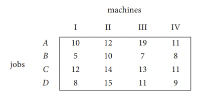
Here the number of rows and columns are equal.

∴ The given assignment problem is balanced. Now let us find the solution.

Step 1: Select a smallest element in each row and subtract this from all the elements in its row.

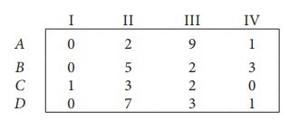
Look for atleast one zero in each row and each column.Otherwise go to step 2.

Step 2: Select the smallest element in each column and subtract this from all the elements in its column.

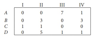
Since each row and column contains atleast one zero, assignments can be made.

Step 3 (Assignment):

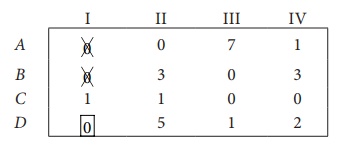
Thus all the four assignments have been made. The optimal assignment schedule and total cost is

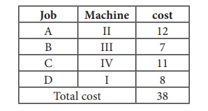
The optimal assignment (minimum) cost

Example 10.8

Consider the problem of assigning five jobs to five persons. The assignment costs are given as follows. Determine the optimum assignment schedule.

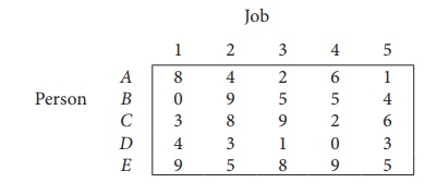
∴ The given assignment problem is balanced.

Now let us find the solution.

The cost matrix of the given assignment problem is

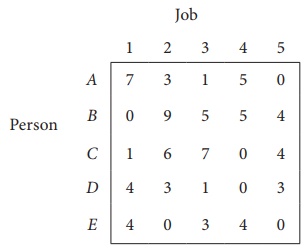
Column 3 contains no zero. Go to Step 2.

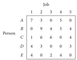
Thus all the five assignments have been made. The Optimal assignment schedule and total cost is

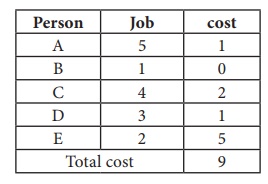
The optimal assignment (minimum) cost = ` 9

Example 10.9

Solve the following assignment problem.

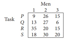
Since the number of columns is less than the number of rows, given assignment problem is unbalanced one. To balance it , introduce a dummy column with all the entries zero. The revised assignment problem is

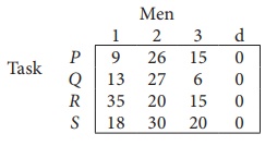
Here only 3 tasks can be assigned to 3 men.

Step 1: is not necessary, since each row contains zero entry. Go to Step 2.

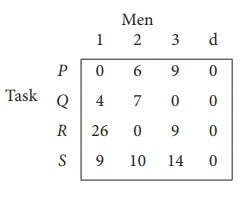
Step 3 (Assignment) :

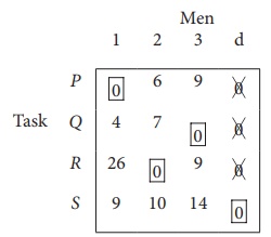
Since each row and each columncontains exactly one assignment,all the three men have been assigned a task. But task S is not assigned to any Man. The optimal assignment schedule and total cost is

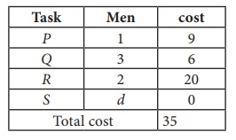
The optimal assignment (minimum) cost = ₹ 35

Related Topics

Privacy Policy , Terms and Conditions , DMCA Policy and Compliant

Copyright © 2018-2024 BrainKart.com; All Rights Reserved. Developed by Therithal info, Chennai.