hypothesis testing p value formula

p-value Calculator

What is p-value, how do i calculate p-value from test statistic, how to interpret p-value, how to use the p-value calculator to find p-value from test statistic, how do i find p-value from z-score, how do i find p-value from t, p-value from chi-square score (χ² score), p-value from f-score.

Welcome to our p-value calculator! You will never again have to wonder how to find the p-value, as here you can determine the one-sided and two-sided p-values from test statistics, following all the most popular distributions: normal, t-Student, chi-squared, and Snedecor's F.

P-values appear all over science, yet many people find the concept a bit intimidating. Don't worry – in this article, we will explain not only what the p-value is but also how to interpret p-values correctly . Have you ever been curious about how to calculate the p-value by hand? We provide you with all the necessary formulae as well!

🙋 If you want to revise some basics from statistics, our normal distribution calculator is an excellent place to start.

Formally, the p-value is the probability that the test statistic will produce values at least as extreme as the value it produced for your sample . It is crucial to remember that this probability is calculated under the assumption that the null hypothesis H 0 is true !

More intuitively, p-value answers the question:

Assuming that I live in a world where the null hypothesis holds, how probable is it that, for another sample, the test I'm performing will generate a value at least as extreme as the one I observed for the sample I already have?

It is the alternative hypothesis that determines what "extreme" actually means , so the p-value depends on the alternative hypothesis that you state: left-tailed, right-tailed, or two-tailed. In the formulas below, S stands for a test statistic, x for the value it produced for a given sample, and Pr(event | H 0 ) is the probability of an event, calculated under the assumption that H 0 is true:

Left-tailed test: p-value = Pr(S ≤ x | H 0 )

Right-tailed test: p-value = Pr(S ≥ x | H 0 )

Two-tailed test:

p-value = 2 × min{Pr(S ≤ x | H 0 ), Pr(S ≥ x | H 0 )}

(By min{a,b} , we denote the smaller number out of a and b .)

If the distribution of the test statistic under H 0 is symmetric about 0 , then: p-value = 2 × Pr(S ≥ |x| | H 0 )

or, equivalently: p-value = 2 × Pr(S ≤ -|x| | H 0 )

As a picture is worth a thousand words, let us illustrate these definitions. Here, we use the fact that the probability can be neatly depicted as the area under the density curve for a given distribution. We give two sets of pictures: one for a symmetric distribution and the other for a skewed (non-symmetric) distribution.

• Symmetric case: normal distribution:

• Non-symmetric case: chi-squared distribution:

In the last picture (two-tailed p-value for skewed distribution), the area of the left-hand side is equal to the area of the right-hand side.

To determine the p-value, you need to know the distribution of your test statistic under the assumption that the null hypothesis is true . Then, with the help of the cumulative distribution function ( cdf ) of this distribution, we can express the probability of the test statistics being at least as extreme as its value x for the sample:

Left-tailed test:

p-value = cdf(x) .

Right-tailed test:

p-value = 1 - cdf(x) .

p-value = 2 × min{cdf(x) , 1 - cdf(x)} .

If the distribution of the test statistic under H 0 is symmetric about 0 , then a two-sided p-value can be simplified to p-value = 2 × cdf(-|x|) , or, equivalently, as p-value = 2 - 2 × cdf(|x|) .

The probability distributions that are most widespread in hypothesis testing tend to have complicated cdf formulae, and finding the p-value by hand may not be possible. You'll likely need to resort to a computer or to a statistical table, where people have gathered approximate cdf values.

Well, you now know how to calculate the p-value, but… why do you need to calculate this number in the first place? In hypothesis testing, the p-value approach is an alternative to the critical value approach . Recall that the latter requires researchers to pre-set the significance level, α, which is the probability of rejecting the null hypothesis when it is true (so of type I error ). Once you have your p-value, you just need to compare it with any given α to quickly decide whether or not to reject the null hypothesis at that significance level, α. For details, check the next section, where we explain how to interpret p-values.

As we have mentioned above, the p-value is the answer to the following question:

What does that mean for you? Well, you've got two options:

• A high p-value means that your data is highly compatible with the null hypothesis; and
• A small p-value provides evidence against the null hypothesis , as it means that your result would be very improbable if the null hypothesis were true.

However, it may happen that the null hypothesis is true, but your sample is highly unusual! For example, imagine we studied the effect of a new drug and got a p-value of 0.03 . This means that in 3% of similar studies, random chance alone would still be able to produce the value of the test statistic that we obtained, or a value even more extreme, even if the drug had no effect at all!

The question "what is p-value" can also be answered as follows: p-value is the smallest level of significance at which the null hypothesis would be rejected. So, if you now want to make a decision on the null hypothesis at some significance level α , just compare your p-value with α :

• If p-value ≤ α , then you reject the null hypothesis and accept the alternative hypothesis; and
• If p-value ≥ α , then you don't have enough evidence to reject the null hypothesis.

Obviously, the fate of the null hypothesis depends on α . For instance, if the p-value was 0.03 , we would reject the null hypothesis at a significance level of 0.05 , but not at a level of 0.01 . That's why the significance level should be stated in advance and not adapted conveniently after the p-value has been established! A significance level of 0.05 is the most common value, but there's nothing magical about it. Here, you can see what too strong a faith in the 0.05 threshold can lead to. It's always best to report the p-value, and allow the reader to make their own conclusions.

Also, bear in mind that subject area expertise (and common reason) is crucial. Otherwise, mindlessly applying statistical principles, you can easily arrive at statistically significant, despite the conclusion being 100% untrue.

As our p-value calculator is here at your service, you no longer need to wonder how to find p-value from all those complicated test statistics! Here are the steps you need to follow:

Pick the alternative hypothesis : two-tailed, right-tailed, or left-tailed.

Tell us the distribution of your test statistic under the null hypothesis: is it N(0,1), t-Student, chi-squared, or Snedecor's F? If you are unsure, check the sections below, as they are devoted to these distributions.

If needed, specify the degrees of freedom of the test statistic's distribution.

Enter the value of test statistic computed for your data sample.

Our calculator determines the p-value from the test statistic and provides the decision to be made about the null hypothesis. The standard significance level is 0.05 by default.

Go to the advanced mode if you need to increase the precision with which the calculations are performed or change the significance level .

In terms of the cumulative distribution function (cdf) of the standard normal distribution, which is traditionally denoted by Φ , the p-value is given by the following formulae:

Left-tailed z-test:

p-value = Φ(Z score )

Right-tailed z-test:

p-value = 1 - Φ(Z score )

Two-tailed z-test:

p-value = 2 × Φ(−|Z score |)

p-value = 2 - 2 × Φ(|Z score |)

🙋 To learn more about Z-tests, head to Omni's Z-test calculator .

We use the Z-score if the test statistic approximately follows the standard normal distribution N(0,1) . Thanks to the central limit theorem, you can count on the approximation if you have a large sample (say at least 50 data points) and treat your distribution as normal.

A Z-test most often refers to testing the population mean , or the difference between two population means, in particular between two proportions. You can also find Z-tests in maximum likelihood estimations.

The p-value from the t-score is given by the following formulae, in which cdf t,d stands for the cumulative distribution function of the t-Student distribution with d degrees of freedom:

Left-tailed t-test:

p-value = cdf t,d (t score )

Right-tailed t-test:

p-value = 1 - cdf t,d (t score )

Two-tailed t-test:

p-value = 2 × cdf t,d (−|t score |)

p-value = 2 - 2 × cdf t,d (|t score |)

Use the t-score option if your test statistic follows the t-Student distribution . This distribution has a shape similar to N(0,1) (bell-shaped and symmetric) but has heavier tails – the exact shape depends on the parameter called the degrees of freedom . If the number of degrees of freedom is large (>30), which generically happens for large samples, the t-Student distribution is practically indistinguishable from the normal distribution N(0,1).

The most common t-tests are those for population means with an unknown population standard deviation, or for the difference between means of two populations , with either equal or unequal yet unknown population standard deviations. There's also a t-test for paired (dependent) samples .

🙋 To get more insights into t-statistics, we recommend using our t-test calculator .

Use the χ²-score option when performing a test in which the test statistic follows the χ²-distribution .

This distribution arises if, for example, you take the sum of squared variables, each following the normal distribution N(0,1). Remember to check the number of degrees of freedom of the χ²-distribution of your test statistic!

How to find the p-value from chi-square-score ? You can do it with the help of the following formulae, in which cdf χ²,d denotes the cumulative distribution function of the χ²-distribution with d degrees of freedom:

Left-tailed χ²-test:

p-value = cdf χ²,d (χ² score )

Right-tailed χ²-test:

p-value = 1 - cdf χ²,d (χ² score )

Remember that χ²-tests for goodness-of-fit and independence are right-tailed tests! (see below)

Two-tailed χ²-test:

p-value = 2 × min{cdf χ²,d (χ² score ), 1 - cdf χ²,d (χ² score )}

(By min{a,b} , we denote the smaller of the numbers a and b .)

The most popular tests which lead to a χ²-score are the following:

Testing whether the variance of normally distributed data has some pre-determined value. In this case, the test statistic has the χ²-distribution with n - 1 degrees of freedom, where n is the sample size. This can be a one-tailed or two-tailed test .

Goodness-of-fit test checks whether the empirical (sample) distribution agrees with some expected probability distribution. In this case, the test statistic follows the χ²-distribution with k - 1 degrees of freedom, where k is the number of classes into which the sample is divided. This is a right-tailed test .

Independence test is used to determine if there is a statistically significant relationship between two variables. In this case, its test statistic is based on the contingency table and follows the χ²-distribution with (r - 1)(c - 1) degrees of freedom, where r is the number of rows, and c is the number of columns in this contingency table. This also is a right-tailed test .

Finally, the F-score option should be used when you perform a test in which the test statistic follows the F-distribution , also known as the Fisher–Snedecor distribution. The exact shape of an F-distribution depends on two degrees of freedom .

To see where those degrees of freedom come from, consider the independent random variables X and Y , which both follow the χ²-distributions with d 1 and d 2 degrees of freedom, respectively. In that case, the ratio (X/d 1 )/(Y/d 2 ) follows the F-distribution, with (d 1 , d 2 ) -degrees of freedom. For this reason, the two parameters d 1 and d 2 are also called the numerator and denominator degrees of freedom .

The p-value from F-score is given by the following formulae, where we let cdf F,d1,d2 denote the cumulative distribution function of the F-distribution, with (d 1 , d 2 ) -degrees of freedom:

Left-tailed F-test:

p-value = cdf F,d1,d2 (F score )

Right-tailed F-test:

p-value = 1 - cdf F,d1,d2 (F score )

Two-tailed F-test:

p-value = 2 × min{cdf F,d1,d2 (F score ), 1 - cdf F,d1,d2 (F score )}

Below we list the most important tests that produce F-scores. All of them are right-tailed tests .

A test for the equality of variances in two normally distributed populations . Its test statistic follows the F-distribution with (n - 1, m - 1) -degrees of freedom, where n and m are the respective sample sizes.

ANOVA is used to test the equality of means in three or more groups that come from normally distributed populations with equal variances. We arrive at the F-distribution with (k - 1, n - k) -degrees of freedom, where k is the number of groups, and n is the total sample size (in all groups together).

A test for overall significance of regression analysis . The test statistic has an F-distribution with (k - 1, n - k) -degrees of freedom, where n is the sample size, and k is the number of variables (including the intercept).

With the presence of the linear relationship having been established in your data sample with the above test, you can calculate the coefficient of determination, R 2 , which indicates the strength of this relationship . You can do it by hand or use our coefficient of determination calculator .

A test to compare two nested regression models . The test statistic follows the F-distribution with (k 2 - k 1 , n - k 2 ) -degrees of freedom, where k 1 and k 2 are the numbers of variables in the smaller and bigger models, respectively, and n is the sample size.

You may notice that the F-test of an overall significance is a particular form of the F-test for comparing two nested models: it tests whether our model does significantly better than the model with no predictors (i.e., the intercept-only model).

Can p-value be negative?

No, the p-value cannot be negative. This is because probabilities cannot be negative, and the p-value is the probability of the test statistic satisfying certain conditions.

What does a high p-value mean?

A high p-value means that under the null hypothesis, there's a high probability that for another sample, the test statistic will generate a value at least as extreme as the one observed in the sample you already have. A high p-value doesn't allow you to reject the null hypothesis.

What does a low p-value mean?

A low p-value means that under the null hypothesis, there's little probability that for another sample, the test statistic will generate a value at least as extreme as the one observed for the sample you already have. A low p-value is evidence in favor of the alternative hypothesis – it allows you to reject the null hypothesis.

Christmas tree

Plant spacing, two envelopes paradox.

• Biology (99)
• Chemistry (98)
• Construction (144)
• Conversion (292)
• Ecology (30)
• Everyday life (261)
• Finance (569)
• Health (440)
• Physics (508)
• Sports (104)
• Statistics (182)
• Other (181)
• Discover Omni (40)

Have a language expert improve your writing

Run a free plagiarism check in 10 minutes, generate accurate citations for free.

• Knowledge Base

Hypothesis Testing | A Step-by-Step Guide with Easy Examples

Published on November 8, 2019 by Rebecca Bevans . Revised on June 22, 2023.

Hypothesis testing is a formal procedure for investigating our ideas about the world using statistics . It is most often used by scientists to test specific predictions, called hypotheses, that arise from theories.

There are 5 main steps in hypothesis testing:

• State your research hypothesis as a null hypothesis and alternate hypothesis (H o ) and (H a  or H 1 ).
• Collect data in a way designed to test the hypothesis.
• Perform an appropriate statistical test .
• Decide whether to reject or fail to reject your null hypothesis.
• Present the findings in your results and discussion section.

Though the specific details might vary, the procedure you will use when testing a hypothesis will always follow some version of these steps.

Table of contents

Step 1: state your null and alternate hypothesis, step 2: collect data, step 3: perform a statistical test, step 4: decide whether to reject or fail to reject your null hypothesis, step 5: present your findings, other interesting articles, frequently asked questions about hypothesis testing.

After developing your initial research hypothesis (the prediction that you want to investigate), it is important to restate it as a null (H o ) and alternate (H a ) hypothesis so that you can test it mathematically.

The alternate hypothesis is usually your initial hypothesis that predicts a relationship between variables. The null hypothesis is a prediction of no relationship between the variables you are interested in.

• H 0 : Men are, on average, not taller than women. H a : Men are, on average, taller than women.

Here's why students love Scribbr's proofreading services

Discover proofreading & editing

For a statistical test to be valid , it is important to perform sampling and collect data in a way that is designed to test your hypothesis. If your data are not representative, then you cannot make statistical inferences about the population you are interested in.

There are a variety of statistical tests available, but they are all based on the comparison of within-group variance (how spread out the data is within a category) versus between-group variance (how different the categories are from one another).

If the between-group variance is large enough that there is little or no overlap between groups, then your statistical test will reflect that by showing a low p -value . This means it is unlikely that the differences between these groups came about by chance.

Alternatively, if there is high within-group variance and low between-group variance, then your statistical test will reflect that with a high p -value. This means it is likely that any difference you measure between groups is due to chance.

Your choice of statistical test will be based on the type of variables and the level of measurement of your collected data .

• an estimate of the difference in average height between the two groups.
• a p -value showing how likely you are to see this difference if the null hypothesis of no difference is true.

Based on the outcome of your statistical test, you will have to decide whether to reject or fail to reject your null hypothesis.

In most cases you will use the p -value generated by your statistical test to guide your decision. And in most cases, your predetermined level of significance for rejecting the null hypothesis will be 0.05 – that is, when there is a less than 5% chance that you would see these results if the null hypothesis were true.

In some cases, researchers choose a more conservative level of significance, such as 0.01 (1%). This minimizes the risk of incorrectly rejecting the null hypothesis ( Type I error ).

Prevent plagiarism. Run a free check.

The results of hypothesis testing will be presented in the results and discussion sections of your research paper , dissertation or thesis .

In the results section you should give a brief summary of the data and a summary of the results of your statistical test (for example, the estimated difference between group means and associated p -value). In the discussion , you can discuss whether your initial hypothesis was supported by your results or not.

In the formal language of hypothesis testing, we talk about rejecting or failing to reject the null hypothesis. You will probably be asked to do this in your statistics assignments.

However, when presenting research results in academic papers we rarely talk this way. Instead, we go back to our alternate hypothesis (in this case, the hypothesis that men are on average taller than women) and state whether the result of our test did or did not support the alternate hypothesis.

If your null hypothesis was rejected, this result is interpreted as “supported the alternate hypothesis.”

These are superficial differences; you can see that they mean the same thing.

You might notice that we don’t say that we reject or fail to reject the alternate hypothesis . This is because hypothesis testing is not designed to prove or disprove anything. It is only designed to test whether a pattern we measure could have arisen spuriously, or by chance.

If we reject the null hypothesis based on our research (i.e., we find that it is unlikely that the pattern arose by chance), then we can say our test lends support to our hypothesis . But if the pattern does not pass our decision rule, meaning that it could have arisen by chance, then we say the test is inconsistent with our hypothesis .

If you want to know more about statistics , methodology , or research bias , make sure to check out some of our other articles with explanations and examples.

• Normal distribution
• Descriptive statistics
• Measures of central tendency
• Correlation coefficient

Methodology

• Cluster sampling
• Stratified sampling
• Types of interviews
• Cohort study
• Thematic analysis

Research bias

• Implicit bias
• Cognitive bias
• Survivorship bias
• Availability heuristic
• Nonresponse bias
• Regression to the mean

Hypothesis testing is a formal procedure for investigating our ideas about the world using statistics. It is used by scientists to test specific predictions, called hypotheses , by calculating how likely it is that a pattern or relationship between variables could have arisen by chance.

A hypothesis states your predictions about what your research will find. It is a tentative answer to your research question that has not yet been tested. For some research projects, you might have to write several hypotheses that address different aspects of your research question.

A hypothesis is not just a guess — it should be based on existing theories and knowledge. It also has to be testable, which means you can support or refute it through scientific research methods (such as experiments, observations and statistical analysis of data).

Null and alternative hypotheses are used in statistical hypothesis testing . The null hypothesis of a test always predicts no effect or no relationship between variables, while the alternative hypothesis states your research prediction of an effect or relationship.

Cite this Scribbr article

If you want to cite this source, you can copy and paste the citation or click the “Cite this Scribbr article” button to automatically add the citation to our free Citation Generator.

Bevans, R. (2023, June 22). Hypothesis Testing | A Step-by-Step Guide with Easy Examples. Scribbr. Retrieved March 22, 2024, from https://www.scribbr.com/statistics/hypothesis-testing/

Is this article helpful?

Rebecca Bevans

Other students also liked, choosing the right statistical test | types & examples, understanding p values | definition and examples.

• Search Search Please fill out this field.

What Is P-Value?

Understanding p-value.

• P-Value in Hypothesis Testing

The Bottom Line

• Corporate Finance
• Financial Analysis

P-Value: What It Is, How to Calculate It, and Why It Matters

Yarilet Perez is an experienced multimedia journalist and fact-checker with a Master of Science in Journalism. She has worked in multiple cities covering breaking news, politics, education, and more. Her expertise is in personal finance and investing, and real estate.

In statistics, a p-value is a number that indicates how likely you are to obtain a value that is at least equal to or more than the actual observation if the null hypothesis is correct.

The p-value serves as an alternative to rejection points to provide the smallest level of significance at which the null hypothesis would be rejected. A smaller p-value means stronger evidence in favor of the alternative hypothesis.

P-value is often used to promote credibility for studies or reports by government agencies. For example, the U.S. Census Bureau stipulates that any analysis with a p-value greater than 0.10 must be accompanied by a statement that the difference is not statistically different from zero. The Census Bureau also has standards in place stipulating which p-values are acceptable for various publications.

Key Takeaways

• A p-value is a statistical measurement used to validate a hypothesis against observed data.
• A p-value measures the probability of obtaining the observed results, assuming that the null hypothesis is true.
• The lower the p-value, the greater the statistical significance of the observed difference.
• A p-value of 0.05 or lower is generally considered statistically significant.
• P-value can serve as an alternative to—or in addition to—preselected confidence levels for hypothesis testing.

Jessica Olah / Investopedia

P-values are usually found using p-value tables or spreadsheets/statistical software. These calculations are based on the assumed or known probability distribution of the specific statistic tested. P-values are calculated from the deviation between the observed value and a chosen reference value, given the probability distribution of the statistic, with a greater difference between the two values corresponding to a lower p-value.

Mathematically, the p-value is calculated using integral calculus from the area under the probability distribution curve for all values of statistics that are at least as far from the reference value as the observed value is, relative to the total area under the probability distribution curve.

The calculation for a p-value varies based on the type of test performed. The three test types describe the location on the probability distribution curve: lower-tailed test, upper-tailed test, or two-tailed test .

In a nutshell, the greater the difference between two observed values, the less likely it is that the difference is due to simple random chance, and this is reflected by a lower p-value.

The P-Value Approach to Hypothesis Testing

The p-value approach to hypothesis testing uses the calculated probability to determine whether there is evidence to reject the null hypothesis. The null hypothesis, also known as the conjecture, is the initial claim about a population (or data-generating process). The alternative hypothesis states whether the population parameter differs from the value of the population parameter stated in the conjecture.

In practice, the significance level is stated in advance to determine how small the p-value must be to reject the null hypothesis. Because different researchers use different levels of significance when examining a question, a reader may sometimes have difficulty comparing results from two different tests. P-values provide a solution to this problem.

Even a low p-value is not necessarily proof of statistical significance, since there is still a possibility that the observed data are the result of chance. Only repeated experiments or studies can confirm if a relationship is statistically significant.

For example, suppose a study comparing returns from two particular assets was undertaken by different researchers who used the same data but different significance levels. The researchers might come to opposite conclusions regarding whether the assets differ.

If one researcher used a confidence level of 90% and the other required a confidence level of 95% to reject the null hypothesis, and if the p-value of the observed difference between the two returns was 0.08 (corresponding to a confidence level of 92%), then the first researcher would find that the two assets have a difference that is statistically significant , while the second would find no statistically significant difference between the returns.

To avoid this problem, the researchers could report the p-value of the hypothesis test and allow readers to interpret the statistical significance themselves. This is called a p-value approach to hypothesis testing. Independent observers could note the p-value and decide for themselves whether that represents a statistically significant difference or not.

Example of P-Value

An investor claims that their investment portfolio’s performance is equivalent to that of the Standard & Poor’s (S&P) 500 Index . To determine this, the investor conducts a two-tailed test.

The null hypothesis states that the portfolio’s returns are equivalent to the S&P 500’s returns over a specified period, while the alternative hypothesis states that the portfolio’s returns and the S&P 500’s returns are not equivalent—if the investor conducted a one-tailed test , the alternative hypothesis would state that the portfolio’s returns are either less than or greater than the S&P 500’s returns.

The p-value hypothesis test does not necessarily make use of a preselected confidence level at which the investor should reset the null hypothesis that the returns are equivalent. Instead, it provides a measure of how much evidence there is to reject the null hypothesis. The smaller the p-value, the greater the evidence against the null hypothesis.

Thus, if the investor finds that the p-value is 0.001, there is strong evidence against the null hypothesis, and the investor can confidently conclude that the portfolio’s returns and the S&P 500’s returns are not equivalent.

Although this does not provide an exact threshold as to when the investor should accept or reject the null hypothesis, it does have another very practical advantage. P-value hypothesis testing offers a direct way to compare the relative confidence that the investor can have when choosing among multiple different types of investments or portfolios relative to a benchmark such as the S&P 500.

For example, for two portfolios, A and B, whose performance differs from the S&P 500 with p-values of 0.10 and 0.01, respectively, the investor can be much more confident that portfolio B, with a lower p-value, will actually show consistently different results.

Is a 0.05 P-Value Significant?

A p-value less than 0.05 is typically considered to be statistically significant, in which case the null hypothesis should be rejected. A p-value greater than 0.05 means that deviation from the null hypothesis is not statistically significant, and the null hypothesis is not rejected.

What Does a P-Value of 0.001 Mean?

A p-value of 0.001 indicates that if the null hypothesis tested were indeed true, then there would be a one-in-1,000 chance of observing results at least as extreme. This leads the observer to reject the null hypothesis because either a highly rare data result has been observed or the null hypothesis is incorrect.

How Can You Use P-Value to Compare 2 Different Results of a Hypothesis Test?

If you have two different results, one with a p-value of 0.04 and one with a p-value of 0.06, the result with a p-value of 0.04 will be considered more statistically significant than the p-value of 0.06. Beyond this simplified example, you could compare a 0.04 p-value to a 0.001 p-value. Both are statistically significant, but the 0.001 example provides an even stronger case against the null hypothesis than the 0.04.

The p-value is used to measure the significance of observational data. When researchers identify an apparent relationship between two variables, there is always a possibility that this correlation might be a coincidence. A p-value calculation helps determine if the observed relationship could arise as a result of chance.

U.S. Census Bureau. “ Statistical Quality Standard E1: Analyzing Data .”

• Terms of Service
• Editorial Policy
• Privacy Policy
• Your Privacy Choices

• Math Article

In Statistics, the researcher checks the significance of the observed result, which is known as test static . For this test, a hypothesis test is also utilized. The P-value  or probability value concept is used everywhere in statistical analysis. It determines the statistical significance and the measure of significance testing. In this article, let us discuss its definition, formula, table, interpretation and how to use P-value to find the significance level etc. in detail.

Table of Contents:

P-value Definition

The P-value is known as the probability value. It is defined as the probability of getting a result that is either the same or more extreme than the actual observations. The P-value is known as the level of marginal significance within the hypothesis testing that represents the probability of occurrence of the given event. The P-value is used as an alternative to the rejection point to provide the least significance at which the null hypothesis would be rejected. If the P-value is small, then there is stronger evidence in favour of the alternative hypothesis.

P-value Table

The P-value table shows the hypothesis interpretations:

Generally, the level of statistical significance is often expressed in p-value and the range between 0 and 1. The smaller the p-value, the stronger the evidence and hence, the result should be statistically significant. Hence, the rejection of the null hypothesis is highly possible, as the p-value becomes smaller.

Let us look at an example to better comprehend the concept of P-value.

Let’s say a researcher flips a coin ten times with the null hypothesis that it is fair. The total number of heads is the test statistic, which is two-tailed. Assume the researcher notices alternating heads and tails on each flip (HTHTHTHTHT). As this is the predicted number of heads, the test statistic is 5 and the p-value is 1 (totally unexceptional).

Assume that the test statistic for this research was the “number of alternations” (i.e., the number of times H followed T or T followed H), which is two-tailed once again. This would result in a test statistic of 9, which is extremely high and has a p-value of 1/2 8 = 1/256, or roughly 0.0039. This would be regarded as extremely significant, much beyond the 0.05 level. These findings suggest that the data set is exceedingly improbable to have happened by random in terms of one test statistic, yet they do not imply that the coin is biased towards heads or tails.

The data have a high p-value according to the first test statistic, indicating that the number of heads observed is not impossible. The data have a low p-value according to the second test statistic, indicating that the pattern of flips observed is extremely unlikely. There is no “alternative hypothesis,” (therefore only the null hypothesis can be rejected), and such evidence could have a variety of explanations – the data could be falsified, or the coin could have been flipped by a magician who purposefully swapped outcomes.

This example shows that the p-value is entirely dependent on the test statistic used and that p-values can only be used to reject a null hypothesis, not to explore an alternate hypothesis.

P-value Formula

We Know that P-value is a statistical measure, that helps to determine whether the hypothesis is correct or not. P-value is a number that lies between 0 and 1. The level of significance(α) is a predefined threshold that should be set by the researcher. It is generally fixed as 0.05. The formula for the calculation for P-value is

Step 1: Find out the test static Z is

P0 = assumed population proportion in the null hypothesis

N = sample size

Step 2: Look at the Z-table to find the corresponding level of P from the z value obtained.

P-Value Example

An example to find the P-value is given here.

Question: A statistician wants to test the hypothesis H 0 : μ = 120 using the alternative hypothesis Hα: μ > 120 and assuming that α = 0.05. For that, he took the sample values as

n =40, σ = 32.17 and x̄ = 105.37. Determine the conclusion for this hypothesis?

We know that,

Now substitute the given values

Now, using the test static formula, we get

t = (105.37 – 120) / 5.0865

Therefore, t = -2.8762

Using the Z-Score table , we can find the value of P(t>-2.8762)

From the table, we get

P (t<-2.8762) = P(t>2.8762) = 0.003

If P(t>-2.8762) =1- 0.003 =0.997

P- value =0.997 > 0.05

Therefore, from the conclusion, if p>0.05, the null hypothesis is accepted or fails to reject.

Hence, the conclusion is “fails to reject H 0. ”

Frequently Asked Questions on P-Value

What is meant by p-value.

The p-value is defined as the probability of obtaining the result at least as extreme as the observed result of a statistical hypothesis test, assuming that the null hypothesis is true.

What does a smaller P-value represent?

The smaller the p-value, the greater the statistical significance of the observed difference, which results in the rejection of the null hypothesis in favour of alternative hypotheses.

What does the p-value greater than 0.05 represent?

If the p-value is greater than 0.05, then the result is not statistically significant.

Can the p-value be greater than 1?

P-value means probability value, which tells you the probability of achieving the result under a certain hypothesis. Since it is a probability, its value ranges between 0 and 1, and it cannot exceed 1.

What does the p-value less than 0.05 represent?

If the p-value is less than 0.05, then the result is statistically significant, and hence we can reject the null hypothesis in favour of the alternative hypothesis.

• Share Share

Register with BYJU'S & Download Free PDFs

Register with byju's & watch live videos.

If you're seeing this message, it means we're having trouble loading external resources on our website.

If you're behind a web filter, please make sure that the domains *.kastatic.org and *.kasandbox.org are unblocked.

To log in and use all the features of Khan Academy, please enable JavaScript in your browser.

AP®︎/College Statistics

Course: ap®︎/college statistics   >   unit 10.

• Idea behind hypothesis testing
• Examples of null and alternative hypotheses
• Writing null and alternative hypotheses
• P-values and significance tests
• Comparing P-values to different significance levels
• Estimating a P-value from a simulation
• Estimating P-values from simulations

Using P-values to make conclusions

• (Choice A)   Fail to reject H 0 ‍   A Fail to reject H 0 ‍  
• (Choice B)   Reject H 0 ‍   and accept H a ‍   B Reject H 0 ‍   and accept H a ‍  
• (Choice C)   Accept H 0 ‍   C Accept H 0 ‍  
• (Choice A)   The evidence suggests that these subjects can do better than guessing when identifying the bottled water. A The evidence suggests that these subjects can do better than guessing when identifying the bottled water.
• (Choice B)   We don't have enough evidence to say that these subjects can do better than guessing when identifying the bottled water. B We don't have enough evidence to say that these subjects can do better than guessing when identifying the bottled water.
• (Choice C)   The evidence suggests that these subjects were simply guessing when identifying the bottled water. C The evidence suggests that these subjects were simply guessing when identifying the bottled water.
• (Choice A)   She would have rejected H a ‍   . A She would have rejected H a ‍   .
• (Choice B)   She would have accepted H 0 ‍   . B She would have accepted H 0 ‍   .
• (Choice C)   She would have rejected H 0 ‍   and accepted H a ‍   . C She would have rejected H 0 ‍   and accepted H a ‍   .
• (Choice D)   She would have reached the same conclusion using either α = 0.05 ‍   or α = 0.10 ‍   . D She would have reached the same conclusion using either α = 0.05 ‍   or α = 0.10 ‍   .
• (Choice A)   The evidence suggests that these bags are being filled with a mean amount that is different than 7.4  kg ‍   . A The evidence suggests that these bags are being filled with a mean amount that is different than 7.4  kg ‍   .
• (Choice B)   We don't have enough evidence to say that these bags are being filled with a mean amount that is different than 7.4  kg ‍   . B We don't have enough evidence to say that these bags are being filled with a mean amount that is different than 7.4  kg ‍   .
• (Choice C)   The evidence suggests that these bags are being filled with a mean amount of 7.4  kg ‍   . C The evidence suggests that these bags are being filled with a mean amount of 7.4  kg ‍   .
• (Choice A)   They would have rejected H a ‍   . A They would have rejected H a ‍   .
• (Choice B)   They would have accepted H 0 ‍   . B They would have accepted H 0 ‍   .
• (Choice C)   They would have failed to reject H 0 ‍   . C They would have failed to reject H 0 ‍   .
• (Choice D)   They would have reached the same conclusion using either α = 0.05 ‍   or α = 0.01 ‍   . D They would have reached the same conclusion using either α = 0.05 ‍   or α = 0.01 ‍   .

Ethics and the significance level α ‍  

Want to join the conversation.

• Upvote Button navigates to signup page
• Downvote Button navigates to signup page
• Flag Button navigates to signup page

7.4.1 - Hypothesis Testing

Five step hypothesis testing procedure.

In the remaining lessons, we will use the following five step hypothesis testing procedure. This is slightly different from the five step procedure that we used when conducting randomization tests. 

• Check assumptions and write hypotheses.  The assumptions will vary depending on the test. In this lesson we'll be confirming that the sampling distribution is approximately normal by visually examining the randomization distribution. In later lessons you'll learn more objective assumptions. The null and alternative hypotheses will always be written in terms of population parameters; the null hypothesis will always contain the equality (i.e., \(=\)).
• Calculate the test statistic.  Here, we'll be using the formula below for the general form of the test statistic.
• Determine the p-value.  The p-value is the area under the standard normal distribution that is more extreme than the test statistic in the direction of the alternative hypothesis.
• Make a decision.  If \(p \leq \alpha\) reject the null hypothesis. If \(p>\alpha\) fail to reject the null hypothesis.
• State a "real world" conclusion.  Based on your decision in step 4, write a conclusion in terms of the original research question.

General Form of a Test Statistic

When using a standard normal distribution (i.e., z distribution), the test statistic is the standardized value that is the boundary of the p-value. Recall the formula for a z score: \(z=\frac{x-\overline x}{s}\). The formula for a test statistic will be similar. When conducting a hypothesis test the sampling distribution will be centered on the null parameter and the standard deviation is known as the standard error.

This formula puts our observed sample statistic on a standard scale (e.g., z distribution). A z score tells us where a score lies on a normal distribution in standard deviation units. The test statistic tells us where our sample statistic falls on the sampling distribution in standard error units.

7.4.1.1 - Video Example: Mean Body Temperature

Research question:  Is the mean body temperature in the population different from 98.6° Fahrenheit?

7.4.1.2 - Video Example: Correlation Between Printer Price and PPM

Research question:  Is there a positive correlation in the population between the price of an ink jet printer and how many pages per minute (ppm) it prints?

7.4.1.3 - Example: Proportion NFL Coin Toss Wins

Research question:  Is the proportion of NFL overtime coin tosses that are won different from 0.50?

StatKey was used to construct a randomization distribution:

Step 1: Check assumptions and write hypotheses

From the given StatKey output, the randomization distribution is approximately normal.

\(H_0\colon p=0.50\)

\(H_a\colon p \ne 0.50\)

Step 2: Calculate the test statistic

\(test\;statistic=\dfrac{sample\;statistic-null\;parameter}{standard\;error}\)

The sample statistic is the proportion in the original sample, 0.561. The null parameter is 0.50. And, the standard error is 0.024.

\(test\;statistic=\dfrac{0.561-0.50}{0.024}=\dfrac{0.061}{0.024}=2.542\)

Step 3: Determine the p value

The p value will be the area on the z distribution that is more extreme than the test statistic of 2.542, in the direction of the alternative hypothesis. This is a two-tailed test:

The p value is the area in the left and right tails combined: \(p=0.0055110+0.0055110=0.011022\)

Step 4: Make a decision

The p value (0.011022) is less than the standard 0.05 alpha level, therefore we reject the null hypothesis.

Step 5: State a "real world" conclusion

There is evidence that the proportion of all NFL overtime coin tosses that are won is different from 0.50

7.4.1.4 - Example: Proportion of Women Students

Research question : Are more than 50% of all World Campus STAT 200 students women?

Data were collected from a representative sample of 501 World Campus STAT 200 students. In that sample, 284 students were women and 217 were not women. 

StatKey was used to construct a sampling distribution using randomization methods:

Because this randomization distribution is approximately normal, we can find the p value by computing a standardized test statistic and using the z distribution.

The assumption here is that the sampling distribution is approximately normal. From the given StatKey output, the randomization distribution is approximately normal. 

\(H_0\colon p=0.50\) \(H_a\colon p>0.50\)

2. Calculate the test statistic

\(test\;statistic=\dfrac{sample\;statistic-hypothesized\;parameter}{standard\;error}\)

The sample statistic is \(\widehat p = 284/501 = 0.567\).

The hypothesized parameter is the value from the hypotheses: \(p_0=0.50\).

The standard error on the randomization distribution above is 0.022.

\(test\;statistic=\dfrac{0.567-0.50}{0.022}=3.045\)

3. Determine the p value

We can find the p value by constructing a standard normal distribution and finding the area under the curve that is more extreme than our observed test statistic of 3.045, in the direction of the alternative hypothesis. In other words, \(P(z>3.045)\):

Our p value is 0.0011634

4. Make a decision

Our p value is less than or equal to the standard 0.05 alpha level, therefore we reject the null hypothesis.

5. State a "real world" conclusion

There is evidence that the proportion of all World Campus STAT 200 students who are women is greater than 0.50.

7.4.1.5 - Example: Mean Quiz Score

Research question:  Is the mean quiz score different from 14 in the population?

\(H_0\colon \mu = 14\)

\(H_a\colon \mu \ne 14\)

The sample statistic is the mean in the original sample, 13.746 points. The null parameter is 14 points. And, the standard error, 0.142, can be found on the StatKey output.

\(test\;statistic=\dfrac{13.746-14}{0.142}=\dfrac{-0.254}{0.142}=-1.789\)

The p value will be the area on the z distribution that is more extreme than the test statistic of -1.789, in the direction of the alternative hypothesis:

This was a two-tailed test. The p value is the area in the left and right tails combined: \(p=0.0368074+0.0368074=0.0736148\)

The p value (0.0736148) is greater than the standard 0.05 alpha level, therefore we fail to reject the null hypothesis.

There is not enough evidence to state that the mean quiz score in the population is different from 14 points. 

7.4.1.6 - Example: Difference in Mean Commute Times

Research question:  Do the mean commute times in Atlanta and St. Louis differ in the population? 

 From the given StatKey output, the randomization distribution is approximately normal.

\(H_0: \mu_1-\mu_2=0\)

\(H_a: \mu_1 - \mu_2 \ne 0\)

Step 2: Compute the test statistic

\(test\;statistic=\dfrac{sample\;statistic - null \; parameter}{standard \;error}\)

The observed sample statistic is \(\overline x _1 - \overline x _2 = 7.14\). The null parameter is 0. And, the standard error, from the StatKey output, is 1.136.

\(test\;statistic=\dfrac{7.14-0}{1.136}=6.285\)

The p value will be the area on the z distribution that is more extreme than the test statistic of 6.285, in the direction of the alternative hypothesis:

This was a two-tailed test. The area in the two tailed combined is 0.000000. Theoretically, the p value cannot be 0 because there is always some chance that a Type I error was committed. This p value would be written as p < 0.001.

The p value is smaller than the standard 0.05 alpha level, therefore we reject the null hypothesis. 

There is evidence that the mean commute times in Atlanta and St. Louis are different in the population. 

Hypothesis Testing

Hypothesis testing is a tool for making statistical inferences about the population data. It is an analysis tool that tests assumptions and determines how likely something is within a given standard of accuracy. Hypothesis testing provides a way to verify whether the results of an experiment are valid.

A null hypothesis and an alternative hypothesis are set up before performing the hypothesis testing. This helps to arrive at a conclusion regarding the sample obtained from the population. In this article, we will learn more about hypothesis testing, its types, steps to perform the testing, and associated examples.

What is Hypothesis Testing in Statistics?

Hypothesis testing uses sample data from the population to draw useful conclusions regarding the population probability distribution . It tests an assumption made about the data using different types of hypothesis testing methodologies. The hypothesis testing results in either rejecting or not rejecting the null hypothesis.

Hypothesis Testing Definition

Hypothesis testing can be defined as a statistical tool that is used to identify if the results of an experiment are meaningful or not. It involves setting up a null hypothesis and an alternative hypothesis. These two hypotheses will always be mutually exclusive. This means that if the null hypothesis is true then the alternative hypothesis is false and vice versa. An example of hypothesis testing is setting up a test to check if a new medicine works on a disease in a more efficient manner.

Null Hypothesis

The null hypothesis is a concise mathematical statement that is used to indicate that there is no difference between two possibilities. In other words, there is no difference between certain characteristics of data. This hypothesis assumes that the outcomes of an experiment are based on chance alone. It is denoted as \(H_{0}\). Hypothesis testing is used to conclude if the null hypothesis can be rejected or not. Suppose an experiment is conducted to check if girls are shorter than boys at the age of 5. The null hypothesis will say that they are the same height.

Alternative Hypothesis

The alternative hypothesis is an alternative to the null hypothesis. It is used to show that the observations of an experiment are due to some real effect. It indicates that there is a statistical significance between two possible outcomes and can be denoted as \(H_{1}\) or \(H_{a}\). For the above-mentioned example, the alternative hypothesis would be that girls are shorter than boys at the age of 5.

Hypothesis Testing P Value

In hypothesis testing, the p value is used to indicate whether the results obtained after conducting a test are statistically significant or not. It also indicates the probability of making an error in rejecting or not rejecting the null hypothesis.This value is always a number between 0 and 1. The p value is compared to an alpha level, \(\alpha\) or significance level. The alpha level can be defined as the acceptable risk of incorrectly rejecting the null hypothesis. The alpha level is usually chosen between 1% to 5%.

Hypothesis Testing Critical region

All sets of values that lead to rejecting the null hypothesis lie in the critical region. Furthermore, the value that separates the critical region from the non-critical region is known as the critical value.

Hypothesis Testing Formula

Depending upon the type of data available and the size, different types of hypothesis testing are used to determine whether the null hypothesis can be rejected or not. The hypothesis testing formula for some important test statistics are given below:

• z = \(\frac{\overline{x}-\mu}{\frac{\sigma}{\sqrt{n}}}\). \(\overline{x}\) is the sample mean, \(\mu\) is the population mean, \(\sigma\) is the population standard deviation and n is the size of the sample.
• t = \(\frac{\overline{x}-\mu}{\frac{s}{\sqrt{n}}}\). s is the sample standard deviation.
• \(\chi ^{2} = \sum \frac{(O_{i}-E_{i})^{2}}{E_{i}}\). \(O_{i}\) is the observed value and \(E_{i}\) is the expected value.

We will learn more about these test statistics in the upcoming section.

Types of Hypothesis Testing

Selecting the correct test for performing hypothesis testing can be confusing. These tests are used to determine a test statistic on the basis of which the null hypothesis can either be rejected or not rejected. Some of the important tests used for hypothesis testing are given below.

Hypothesis Testing Z Test

A z test is a way of hypothesis testing that is used for a large sample size (n ≥ 30). It is used to determine whether there is a difference between the population mean and the sample mean when the population standard deviation is known. It can also be used to compare the mean of two samples. It is used to compute the z test statistic. The formulas are given as follows:

• One sample: z = \(\frac{\overline{x}-\mu}{\frac{\sigma}{\sqrt{n}}}\).
• Two samples: z = \(\frac{(\overline{x_{1}}-\overline{x_{2}})-(\mu_{1}-\mu_{2})}{\sqrt{\frac{\sigma_{1}^{2}}{n_{1}}+\frac{\sigma_{2}^{2}}{n_{2}}}}\).

Hypothesis Testing t Test

The t test is another method of hypothesis testing that is used for a small sample size (n < 30). It is also used to compare the sample mean and population mean. However, the population standard deviation is not known. Instead, the sample standard deviation is known. The mean of two samples can also be compared using the t test.

• One sample: t = \(\frac{\overline{x}-\mu}{\frac{s}{\sqrt{n}}}\).
• Two samples: t = \(\frac{(\overline{x_{1}}-\overline{x_{2}})-(\mu_{1}-\mu_{2})}{\sqrt{\frac{s_{1}^{2}}{n_{1}}+\frac{s_{2}^{2}}{n_{2}}}}\).

Hypothesis Testing Chi Square

The Chi square test is a hypothesis testing method that is used to check whether the variables in a population are independent or not. It is used when the test statistic is chi-squared distributed.

One Tailed Hypothesis Testing

One tailed hypothesis testing is done when the rejection region is only in one direction. It can also be known as directional hypothesis testing because the effects can be tested in one direction only. This type of testing is further classified into the right tailed test and left tailed test.

Right Tailed Hypothesis Testing

The right tail test is also known as the upper tail test. This test is used to check whether the population parameter is greater than some value. The null and alternative hypotheses for this test are given as follows:

\(H_{0}\): The population parameter is ≤ some value

\(H_{1}\): The population parameter is > some value.

If the test statistic has a greater value than the critical value then the null hypothesis is rejected

Left Tailed Hypothesis Testing

The left tail test is also known as the lower tail test. It is used to check whether the population parameter is less than some value. The hypotheses for this hypothesis testing can be written as follows:

\(H_{0}\): The population parameter is ≥ some value

\(H_{1}\): The population parameter is < some value.

The null hypothesis is rejected if the test statistic has a value lesser than the critical value.

Two Tailed Hypothesis Testing

In this hypothesis testing method, the critical region lies on both sides of the sampling distribution. It is also known as a non - directional hypothesis testing method. The two-tailed test is used when it needs to be determined if the population parameter is assumed to be different than some value. The hypotheses can be set up as follows:

\(H_{0}\): the population parameter = some value

\(H_{1}\): the population parameter ≠ some value

The null hypothesis is rejected if the test statistic has a value that is not equal to the critical value.

Hypothesis Testing Steps

Hypothesis testing can be easily performed in five simple steps. The most important step is to correctly set up the hypotheses and identify the right method for hypothesis testing. The basic steps to perform hypothesis testing are as follows:

• Step 1: Set up the null hypothesis by correctly identifying whether it is the left-tailed, right-tailed, or two-tailed hypothesis testing.
• Step 2: Set up the alternative hypothesis.
• Step 3: Choose the correct significance level, \(\alpha\), and find the critical value.
• Step 4: Calculate the correct test statistic (z, t or \(\chi\)) and p-value.
• Step 5: Compare the test statistic with the critical value or compare the p-value with \(\alpha\) to arrive at a conclusion. In other words, decide if the null hypothesis is to be rejected or not.

Hypothesis Testing Example

The best way to solve a problem on hypothesis testing is by applying the 5 steps mentioned in the previous section. Suppose a researcher claims that the mean average weight of men is greater than 100kgs with a standard deviation of 15kgs. 30 men are chosen with an average weight of 112.5 Kgs. Using hypothesis testing, check if there is enough evidence to support the researcher's claim. The confidence interval is given as 95%.

Step 1: This is an example of a right-tailed test. Set up the null hypothesis as \(H_{0}\): \(\mu\) = 100.

Step 2: The alternative hypothesis is given by \(H_{1}\): \(\mu\) > 100.

Step 3: As this is a one-tailed test, \(\alpha\) = 100% - 95% = 5%. This can be used to determine the critical value.

1 - \(\alpha\) = 1 - 0.05 = 0.95

0.95 gives the required area under the curve. Now using a normal distribution table, the area 0.95 is at z = 1.645. A similar process can be followed for a t-test. The only additional requirement is to calculate the degrees of freedom given by n - 1.

Step 4: Calculate the z test statistic. This is because the sample size is 30. Furthermore, the sample and population means are known along with the standard deviation.

z = \(\frac{\overline{x}-\mu}{\frac{\sigma}{\sqrt{n}}}\).

\(\mu\) = 100, \(\overline{x}\) = 112.5, n = 30, \(\sigma\) = 15

z = \(\frac{112.5-100}{\frac{15}{\sqrt{30}}}\) = 4.56

Step 5: Conclusion. As 4.56 > 1.645 thus, the null hypothesis can be rejected.

Hypothesis Testing and Confidence Intervals

Confidence intervals form an important part of hypothesis testing. This is because the alpha level can be determined from a given confidence interval. Suppose a confidence interval is given as 95%. Subtract the confidence interval from 100%. This gives 100 - 95 = 5% or 0.05. This is the alpha value of a one-tailed hypothesis testing. To obtain the alpha value for a two-tailed hypothesis testing, divide this value by 2. This gives 0.05 / 2 = 0.025.

Related Articles:

• Probability and Statistics
• Data Handling

Important Notes on Hypothesis Testing

• Hypothesis testing is a technique that is used to verify whether the results of an experiment are statistically significant.
• It involves the setting up of a null hypothesis and an alternate hypothesis.
• There are three types of tests that can be conducted under hypothesis testing - z test, t test, and chi square test.
• Hypothesis testing can be classified as right tail, left tail, and two tail tests.

Examples on Hypothesis Testing

• Example 1: The average weight of a dumbbell in a gym is 90lbs. However, a physical trainer believes that the average weight might be higher. A random sample of 5 dumbbells with an average weight of 110lbs and a standard deviation of 18lbs. Using hypothesis testing check if the physical trainer's claim can be supported for a 95% confidence level. Solution: As the sample size is lesser than 30, the t-test is used. \(H_{0}\): \(\mu\) = 90, \(H_{1}\): \(\mu\) > 90 \(\overline{x}\) = 110, \(\mu\) = 90, n = 5, s = 18. \(\alpha\) = 0.05 Using the t-distribution table, the critical value is 2.132 t = \(\frac{\overline{x}-\mu}{\frac{s}{\sqrt{n}}}\) t = 2.484 As 2.484 > 2.132, the null hypothesis is rejected. Answer: The average weight of the dumbbells may be greater than 90lbs
• Example 2: The average score on a test is 80 with a standard deviation of 10. With a new teaching curriculum introduced it is believed that this score will change. On random testing, the score of 38 students, the mean was found to be 88. With a 0.05 significance level, is there any evidence to support this claim? Solution: This is an example of two-tail hypothesis testing. The z test will be used. \(H_{0}\): \(\mu\) = 80, \(H_{1}\): \(\mu\) ≠ 80 \(\overline{x}\) = 88, \(\mu\) = 80, n = 36, \(\sigma\) = 10. \(\alpha\) = 0.05 / 2 = 0.025 The critical value using the normal distribution table is 1.96 z = \(\frac{\overline{x}-\mu}{\frac{\sigma}{\sqrt{n}}}\) z = \(\frac{88-80}{\frac{10}{\sqrt{36}}}\) = 4.8 As 4.8 > 1.96, the null hypothesis is rejected. Answer: There is a difference in the scores after the new curriculum was introduced.
• Example 3: The average score of a class is 90. However, a teacher believes that the average score might be lower. The scores of 6 students were randomly measured. The mean was 82 with a standard deviation of 18. With a 0.05 significance level use hypothesis testing to check if this claim is true. Solution: The t test will be used. \(H_{0}\): \(\mu\) = 90, \(H_{1}\): \(\mu\) < 90 \(\overline{x}\) = 110, \(\mu\) = 90, n = 6, s = 18 The critical value from the t table is -2.015 t = \(\frac{\overline{x}-\mu}{\frac{s}{\sqrt{n}}}\) t = \(\frac{82-90}{\frac{18}{\sqrt{6}}}\) t = -1.088 As -1.088 > -2.015, we fail to reject the null hypothesis. Answer: There is not enough evidence to support the claim.

go to slide go to slide go to slide

Book a Free Trial Class

FAQs on Hypothesis Testing

What is hypothesis testing.

Hypothesis testing in statistics is a tool that is used to make inferences about the population data. It is also used to check if the results of an experiment are valid.

What is the z Test in Hypothesis Testing?

The z test in hypothesis testing is used to find the z test statistic for normally distributed data . The z test is used when the standard deviation of the population is known and the sample size is greater than or equal to 30.

What is the t Test in Hypothesis Testing?

The t test in hypothesis testing is used when the data follows a student t distribution . It is used when the sample size is less than 30 and standard deviation of the population is not known.

What is the formula for z test in Hypothesis Testing?

The formula for a one sample z test in hypothesis testing is z = \(\frac{\overline{x}-\mu}{\frac{\sigma}{\sqrt{n}}}\) and for two samples is z = \(\frac{(\overline{x_{1}}-\overline{x_{2}})-(\mu_{1}-\mu_{2})}{\sqrt{\frac{\sigma_{1}^{2}}{n_{1}}+\frac{\sigma_{2}^{2}}{n_{2}}}}\).

What is the p Value in Hypothesis Testing?

The p value helps to determine if the test results are statistically significant or not. In hypothesis testing, the null hypothesis can either be rejected or not rejected based on the comparison between the p value and the alpha level.

What is One Tail Hypothesis Testing?

When the rejection region is only on one side of the distribution curve then it is known as one tail hypothesis testing. The right tail test and the left tail test are two types of directional hypothesis testing.

Professor McCarthy Statistics

Mat 150 bmcc, 10. hypothesis testing: p-values, exact binomial test, simple one-sided claims about proportions, the following 8 videos (run times vary from 2 to 8 minutes) will help you with your blackboard homework on this unit..

Please scroll down past these homework videos for an in depth explanation of Hypothesis Testing & P-values.

Question 2 and 3.

See Questions 4, 5, and 6, towards the bottom of this page for R scripts to calculate the p-value and a barplot for simple claims about proportions.

There are 2 videos at the end of Question 1 below.

A hypothesis is a claim about a population.

Examples of hypotheses:

• Claim: more than 60% of students like math.
• Claim: the mean weight of cats is less than 9 pounds

We test a claim by taking a sample from the population. If the data from the sample agrees with (or supports ) the claim, we say the data provides evidence that the claim is true.

• Claim : more than 60% of students like math.  $\rho > 60\%$ Data : If in a sample of 10 students 8 of them like math, the sample supports the claim because $\dfrac{8}{10} = 80\% > 60\%$. If 9 of the 10 liked math, the sample would provide even stronger support because 90% > 80% > 60%. If 6 of the 10 liked math, that data doesn’t support the claim since $\dfrac{6}{10} = 60\%$ is not more than 60%.
• Claim : the mean weight of cats is less than 9 pounds.  $\mu < 9 \text{ pounds }$ Data : If in a sample of 30 cats the mean weight was 8 pounds, the sample supports the claim because 8 pounds < 9 pounds. If in that sample the mean weight was 6 pounds, it would provide even stronger support of the claim because 6 pounds < 8 pounds < 9 pounds.

If the data from the sample supports the claim we can conduct a formal hypothesis test to determine if the sample provides statistically significant evidence that the claim is true.

After Question 7 (below) is a section on how to report the results of a hypothesis test .

p-value method of hypothesis testing

The p-value concept is difficult to understand at first. My suggestion is to read these definitions and descriptions. Then read through the first two or three Questions and their solutions. Then read these definitions again.

Definition . The sample used in the hypothesis test is called the test-sample .

Definition . The p-value is the maximum probability of getting a sample that provides as much support for the claim as the test-sample if we assume that the claim is false.

Note. “ as much support ” means the same or stronger support.

So, if the p-value is small, it would be very unlikely for us to get a sample which provides as much support for the claim being true, as the test-sample does, if the claim were false. So, if the p-value is small, the test-sample provides good evidence that the claim wasn’t false. So, a small p-value indicates the test-sample should be considered significant (strong) evidence that the claim is true.

WARNING!!! When we calculate a p-value it is with respect to a mathematical model of the “experiment”. The better the  model represents the experimental design, the sampling method, etc., the more relevant will be the p-value. Think about it. Unless the model faithfully represents the experiment, the p-value we calculate will tell us nothing meaningful. For more on this, please read the section, in Question 1 below, called: Important aside about mathematical models.

General algorithm to calculate the p-value:

If the claim is false, the maximum probability of getting a sample which supports the claim happens if the claim is false by the smallest amount possible. Think: little lies are difficult to detect.

So, to calculate the p-value we assume the claim is false by the smallest amount possible and then we calculate the probability of getting a sample that provides as much support as the test-sample.

How small does the p-value have to be in order for it indicate that the test-sample provides significant (strong) evidence that the claim is true?

Definition . If the p-value is smaller than a number called the level of significance , denoted $\alpha$, we say the sample provides statistically significant (strong) evidence that the claim is true.

Unless otherwise noted, in these notes we will always assume that $\alpha = 0.05$ as that is the most common value for  $\alpha$.

Type I and type II errors

Type I and type II errors . The definition of the  p-value is often given in terms of a concept called a type I error . A type I error is when a false claim is accepted as true. A type II error is when a true claim is rejected as false  1 .

We can define the p-value as: the maximum probability of making type I error, if we are willing to accept the claim as true whenever we get a sample that provides as much support as the test-sample.

Important notes about p-values

• Since p-values are a probability we always have $0 \leq \text{ p-value } \leq 1$.
• A small p-value doesn’t mean the claim is true, or even likely to be true .
• A large p-value means the data in the sample should not be reported as evidence of the claim being true.

The p-value method of hypothesis testing is probably the most common way to test a claim. It also is probably the most misunderstood concept in statistics.

The best way to understand the concept of a p-value is to learn how to calculate the p-value for a simple claim where the mathematics is not too difficult: the exact binomial test (see below). Other types of claims will have more complicated ways of calculating the p-value, but the meaning of the p-value doesn’t change.

P-value method of hypothesis testing for simple one-sided claims about a proportion. The Exact Binomial Test

A simple one-sided claim about a proportion is a claim that a proportion is greater than some percent or less than some percent.

The symbol for proportion is $\rho$.

The name of the hypothesis test that we use for this situation is “ the exact binomial test “.  Binomial because we use the binomial distribution. Exact because we don’t approximate the binomial distribution by a continuous distribution.

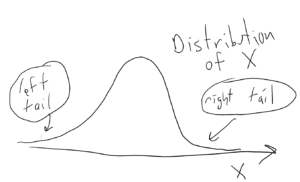
Note. Generally speaking, we test one-sided claims with one-tailed tests. The term “one-tailed” comes from the p-value being the area in one of the “tails” of the distribution.  See Figures below and the Figures accompanying the answers to Questions 1 through 6.

Question 1. 

Using the p-value method of hypothesis testing test the following claim at the $\alpha = 0.05$ significance level.

• Claim: More than 60% of students are STEM majors.
• Data:  In a sample of 10 students 8 of them are STEM majors.

Answer to Question 1. (Also, see video below).

• $n = $ the size of our sample, so $n = 10$.
• $X = $ the random variable that counts how many of the students in such samples ($n = 10$) are stem majors. $X(\text{our sample}) = 8$
• $\rho = $ “the true proportion of students in the population who are STEM majors”.

The sample’s proportion $\hat{p}$ of STEM majors is $$\hat{p} = \dfrac{X(\text{our sample})}{n} = \dfrac{8}{10} = 80\%$$ which supports our claim because $80\% > 60\%$.

Since the sample supports the claim, we conduct the hypothesis test and calculate the p-value.

In a formal hypothesis test we write the alternative and null hypotheses at the start of the problem. For us, $H_A$ (the alternative hypothesis) will always be the claim and $H_0$ (the null hypothesis) will always be the assumption for the parameters that we will use for our p-value calculation (basically that the claim is false in the smallest way possible):

$\text{(claim) } \ H_A: \rho > 60\%$ $\text{(null) } \ H_0: \rho = 60\%$

Important aside about mathematical models. For simple claims about a proportions, like in Question 1, we model the sampling process as a Bernoulli process having a binomial distribution. When we calculate a p-value it is with respect to the model, not to the actual experiment. The closer the  experimental design is  is to the model, the more relevant will be the p-value. Think about it. Suppose we have some real-life claim that we are testing. To save money, we could just make up the data and calculate the p-value; or we could collect the data in a sloppy manner, or make a mess of the data in a million ways; but what would a p-value based on such data tell us about the real world? Absolutely nothing.

T o calculate the p-value we assume the claim is false by the smallest amount possible and then we calculate the probability of getting a sample that provides as much support as the test-sample.

$X(\text{test-sample}) = 8$ so samples that provide as much support are samples which satisfy $X = 8, 9$, or $10$.

$$\text{p-value} = P(X \geq 8 \ \mid \rho = 60\%)$$

Notation.   $P(X \geq 8 \ \mid \rho = 60\%)$ means:

$P(X \geq 8)$ assuming that $\rho = 60\%$

Note. The assumption that $\rho = 60\%$ is the null hypothesis $H_0$. Also, see  footnote  2 on $P(A\mid B)$ and Conditional Probability.

As mentioned above, we model our claim and the sampling process as being a Bernoulli process having a binomial distribution with n = 10 and $\rho = 60\%$.  Other types of claims and sampling methods will have different mathematical models and involve different types of distributions.

Recall the binomial distribution formula:

$$P(X = r) = nCr\ \rho^r \ (1 – \rho)^{n-r}$$

Substituting in $n = 10$ and $\rho = 60\%$ we finally, actually calculate the p-value:

$\text{p-value} = P(X \geq 8 \  \mid \rho = 60\%)$ $ = P(X = 8) + P(X=9) + P(X= 10) $ $ = 10C8\ (60\%)^8 \ (40\%)^{2} $ $+ 10C9\ (60\%)^9 \ (40\%)^{1} $ $+ 10C10\ (60\%)^{10} \ (40\%)^{0}$ $=0.1209324 + 0.04031078 + 0.006046618$ $ = 0.1672898$

So, the p-value = 0.1672898.

Statistical significance.   If the p-value is LESS THAN the significance level $\alpha$ we can report:

• the sample provides statistically significant evidence that the claim is true, or
• the result of the study is statistically significant.

Result. Since the

(p-value = .1672898)   >   ($\alpha = .05$)

the sample doesn’t provide statistically significant evidence that the claim is true (at the $\alpha = 0.05$ significance level).

Note . In the above calculation, $ P(X = 8) + P(X=9) + P(X= 10) $ are all done with the assumption that $\rho = 60\%$.

Extremely important geometric interpretation of the p-value See barplot Figure below

Here is the probability density barplot corresponding to the p-value calculated in Question 1, above:

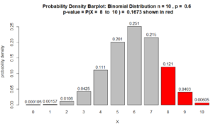
Figure for Question 1. The p-value is the area of the red bars.

For many statisticians, the above Figure is what explains the p-value. As the data from the sample provides more support, the p-value, which is the area of the red bars, decreases. See, for example, Question 2 below.

Note about the above barplot. The heights of the bars are probability densities and the areas of the bars are probabilities . Area = width $\times$ height. Since the bars’ widths are 1, the area of the bars are numerically equivalent to their height. In other words, the numbers on top of the bars are also probabilities. So, for example $P(X=8) = 0.121$.

So, we’ve finished Question 1.

Video showing how to solve Question 1 above (9:35):

Video for Question 1.

Continuation of above video showing solution to Question 2 below (3:34).

Video for Question 1 and 2 showing barplot.

Question 2: Redo the hypothesis test from Question 1, if $X(\text{our sample})$ had been 9, instead of 8. As in Question 1, the sample size is $n =10$ and the level of significance to be used is $\alpha = 0.05$.

Answer to Question 2:

• $X = $ the random variable that counts how many of the students in such samples are stem majors. $X(\text{our sample}) = 9$

The sample’s proportion $\hat{p}$ of STEM majors is $$\hat{p} = \dfrac{X(\text{our sample})}{n} = \dfrac{9}{10} = 90\%$$ which supports our claim because $80\% > 60\%$.

$\text{p-value} = P(X \geq 9 \  \mid \rho = 60\%)$ $ = P(X=9) + P(X= 10) $ $+ 10C9\ (60\%)^9 \ (40\%)^{1} $ $+ 10C10\ (60\%)^{10} \ (40\%)^{0}$ $= 0.04031078 + 0.006046618$ $ = 0.0463574$

which indicates statistical significance because 0.0463574 < 0.05. Also, see Figure below.

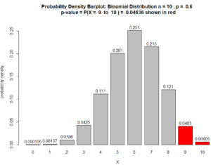
Figure for Question 2. The p-value is the area of the red bars.

Question 3. 

• Claim: Less than 60% of students are STEM majors.
• Data:  In a sample of 10 students 2 of them are STEM majors.

Answer to Question 3 .

• $X = $ the random variable that counts how many of the students in such samples are stem majors. $X(\text{our sample}) = 2$

The sample’s proportion $\hat{p}$ of STEM majors is $$\hat{p} = \dfrac{X(\text{our sample})}{n} = \dfrac{2}{10} = 20\%$$ which supports our claim because $20\% < 60\%$.

$\text{(claim) } \ H_A: \rho < 60\%$ $\text{(null) } \ H_0: \rho = 60\%$

$\text{p-value} = P(X \leq 2 \  \mid \rho = 60\%)$ $ = P(X=0) + P(X= 1) + P(X= 2) $ $+ 10C0\ (60\%)^0 \ (40\%)^{10} $ $+ 10C1\ (60\%)^1 \ (40\%)^{9}$ $+ 10C2\ (60\%)^2\ (40\%)^{8}$ $= 0.0001048576 +  0.001572864 +  0.010616832$ $ = 0.01229$

which indicates statistical significance because the

(p-value = .01229)   <   ($\alpha = 0.05$)

Also, see Figure below.

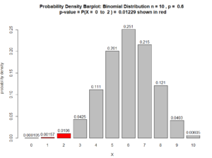
Figure for Question 3. The p-value is the area of the red bars.

Question 4. 

• Claim: Less than 49% of children play baseball.
• Data:  In a sample of 12 children 3 of them play baseball.

Answer to Question 4 .

• $n = $ the size of our sample, so $n = 12$.
• $X = $ the random variable that counts how many of the children in such samples are baseball players. $X(\text{our sample}) = 3$
• $\rho = $ “the true proportion of children in the population who play baseball”.

The sample’s proportion $\hat{p}$ of baseball players is $$\hat{p} = \dfrac{X(\text{our sample})}{n} = \dfrac{3}{12} = 25\%$$ which supports our claim because $25\% < 49\%$.

$\text{(claim) } \ H_A: \rho < 49\%$ $\text{(null) } \ H_0: \rho = 49\%$

$\text{p-value} = P(X \leq 3 \  \mid \rho = 49\%)$ $ = P(X=0) + P(X= 1) + P(X= 2) + P(X=3) $ $+ 12C0\ (49\%)^0 \ (51\%)^{12} $ $+ 12C1\ (49\%)^1 \ (51\%)^{11}$ $+ 10C2\ (49\%)^2\ (51\%)^{10}$ $+ 10C3\ (49\%)^3\ (51\%)^{9}$ $= 0.000309629344375621 $ $+ 0.00356984420574246 $ $+ 0.0188641767342666$ $+ 0.0604146836587622$ $ = 0.08316$

which indicates NO statistical significance because the

(p-value = .08316)   >   ($\alpha = 0.05$)

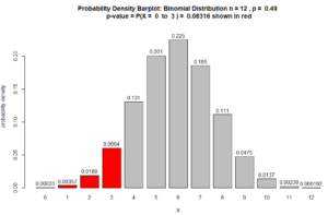
Figure for Question 4. The p-value is the area of the red bars.

Here is the R script used to create the above barplot.

The above script also outputs the distribution of $X$ to the “R Console” window:

Question 5. 

• Claim: More than 55% of children play baseball.
• Data:  In a sample of 12 children 10  of them play baseball.

Answer to Question 5 .

• $X = $ the random variable that counts how many of the children in such samples are baseball players. $X(\text{our sample}) = 10$

The sample’s proportion $\hat{p}$ of baseball players is $$\hat{p} = \dfrac{X(\text{our sample})}{n} = \dfrac{10}{12} = 83.3\%$$ which supports our claim because $83.3\%  > 55\%$.

$\text{(claim) } \ H_A: \rho > 55\%$ $\text{(null) } \ H_0: \rho = 55\%$

$\text{p-value} = P(X \geq 10 \  \mid \rho = 55\%)$ $ = P(X=10) + P(X= 11) + P(X= 12) $ $+ 12C10\ (55\%)^{10} \ (45\%)^{2} $ $+ 12C11\ (55\%)^{11} \ (45\%)^{1}$ $+ 12C12\ (55\%)^{12}\ (45\%)^{0}$ $= 0.0338528984172231$ $+ 0.00752286631493849$ $+ 0.000766217865410401$ $ = 0.04214$

which indicates the sample provides statistically significant evidence that the claim is true because the

(p-value = .04214)   <   ($\alpha = 0.05$)

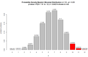
Figure for Question 5. The p-value is the area of the red bars.

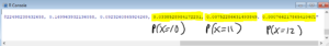
Question 6. 

• Claim: More than 51% of children like chocolate.
• Data:  In a sample of 200 children 115  of them like chocolate.

Answer to Question 6 .

• $n = $ the size of our sample, so $n = 200$.
• $X = $ the random variable that counts how many of the children in such samples like chocolate. $X(\text{our sample}) = 115$
• $\rho = $ “the true proportion of children that like chocolate”.

The sample’s proportion $\hat{p}$ of children who like chocolate is $$\hat{p} = \dfrac{X(\text{our sample})}{n} = \dfrac{115}{200} = 57.5\%$$ which supports our claim because $57.5\%  > 51\%$.

$\text{(claim) } \ H_A: \rho > 51\%$ $\text{(null) } \ H_0: \rho = 51\%$

(The following calculation was too long to be done by hand. So I used R.)

$\text{p-value} = P(X \geq 115 \  \mid \rho = 51\%)$ $ = P(X=115) + P(X= 116) + \cdots +  P(X= 200) $ $+ 200C115\ (51\%)^{115} \ (49\%)^{85} $ $+ 200C116\ (51\%)^{116} \ (49\%)^{84}$ $\vdots$ $+ 200C200\ (51\%)^{200}\ (49\%)^{0}$ $= 0.010427568 $ $+ 0.007952763$ $\vdots$ $+ 3.266143\times 10^{-59}$ $ = 0.0383$

(p-value = .0383)   <   ($\alpha = .05$)

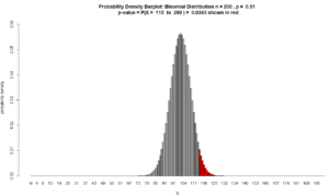
Figure for Question 6. The p-value is the area of the red bars.

Here is the R script used to create the above barplot. Since the bars are very thin, if we put numbers on top of them, the result will be a mess. So, this script omits the numbers on top of the bars.

If we just want to calculate the p-value, the script is much simpler:

Question 7. 

• Data:  In a sample of 200 children 100  of them like chocolate.

Answer to Question 7 .

• $X = $ the random variable that counts how many of the children in such samples like chocolate. $X(\text{our sample}) = 100$

The sample’s proportion $\hat{p}$ of children who like chocolate is $$\hat{p} = \dfrac{X(\text{our sample})}{n} = \dfrac{100}{200} = 50\%$$ which doesn’t support our claim.

The data is contrary to the claim, so we don’t have to calculate the p-value.

End of Question 7.

How to report these results in a scientific paper.

Each journal has its own style for how authors should report their results.

If the sample provided statistical significance , like in Question 6, the authors might write  something like:

More than 51% of children like chocolate (p = .0383, exact binomial test).

In our survey of 200 children, 57.5% liked chocolate, suggesting more than 51% of children like chocolate (p = .0308, exact binomial test).

The author’s won’t say they did a hypothesis test. They will often state the claim as if it were a fact (even though it isn’t). When they put the p-value they typically leave off the leading zero, so 0.0383 becomes .0383. Also, rather than write p-value, authors typically just write p. The authors won’t usually say that the results are statistically significant: the p-value being less than 0.05 indicates that. Finally, authors should name the type of hypothesis test that they used. In these examples the exact binomial test was used.

If the sample failed to provide statistical significance , for example, if in Question 6 we had $X = 104$, so that $\hat{p} = \dfrac{104}{200} = 52\%$, the p-value would be:

$$\text{p-value } = P(X \geq 104 \mid \rho = 51\%)  = .4162$$

If the authors wanted to include this inconclusive result in their paper, they might write something like:

As to the belief that more than 51% of children like chocolate: in our survey of 200 children, 52% said they liked chocolate, which not statistically significant (p = .4162, exact binomial test).

Based on our experiences with children, we expected that more than 51% of children would like chocolate: in our survey of 200 children, 52% said they liked chocolate, however this was not statistically significant (exact binomial test).

If the sample provided evidence contrary to the claim , like in Question 7 where we had $X = 100$ so that $\hat{p} = \dfrac{100}{200} = 50\%$  we wouldn’t bother to calculate the p-value (since the sample doesn’t support the claim).

It the authors wanted to include this contrary result, the authors might write something like:

We had thought that more than 51% of children liked chocolate. However, when we surveyed 200 children we found that only 50% said they liked chocolate.

An interesting way to think about the p-value.

• In some sense, the p-value measures how gullible you need to be in order to accept the claim as true based on the data in a sample. So, a smaller p-value indicates you’d need to be less gullible to accept the claim.

How a p-value should be used in the real world

• If the p-value is small, your doubts about the claim being true should be based more on the experimental design, or on an improperly chosen model, or that the authors used the wrong type of hypothesis test; rather than on things like the sample size being too small, or that, due to chance, getting a misleading sample.  Note. A small sample size will often result in a large p-value.
• A small p-value doesn’t mean that the claim is true, or is even likely to be true.
• A large p-value doesn’t mean the  claim is false.
• A large p-value means the data in the sample should not be presented as evidence of the claim being true.
• Different scientific fields will use different levels of significance to determine if the p-value is small or large, and whether the study can be reported as being “statistically significant”. In these notes we will always use a level of significance of $\alpha = 0.05$ because that is the most  commonly used value.

If we have to decide whether to accept a claim as true, there are two ways we could make a mistake or error.

• Type I Error .  A type I error is when a false claim is accepted as true. Type I errors are made by people who are too trusting and gullible.
• Type II Error .  A type II error is when we fail to accept a true claim. Type II errors are made by people who are too cynical.

$P(A \mid B)$ is read as the “probability of A assuming B”.

Example . Suppose $X$ is a binomally distributed random variable with $n = 10$. If we write

$$P(X = 8 \mid \rho = 60\%)$$

what we mean is

“the probability that $X = 8$ assuming that $\rho = 60\%$”.

Applying the binomial distribution formula we get:

$P(X = 8 \mid \rho = 60\%)$ $= 10C8\, \rho^8 (1 – \rho)^2$ $= 10C8\, (.60)^8 (.40)^2 $ $= 0.1209324$

Same example continued . Since $n = 10$ we have: $$P(X \geq 9 \mid \rho = 60\%) = P(X = 9 \mid \rho = 60\%) + P(X = 10 \mid \rho = 60\%)$$ However, the above is a little bit long, so to save space, we might write: $$P(X \geq 9 \mid \rho = 60\%) = P(X = 9) + P(X = 10)$$ where, in the above,  $P(X = 9)$ means  $P(X = 9 \mid \rho = 60\%)$ and  $P(X = 10)$  means  $P(X = 10 \mid \rho = 60\%)$.

Conditional probability uses the same notation $P(A \mid B)$.

Definition of conditional probability:

$$P(A \mid B) =   \dfrac{P(A \cap B}{P(B)}$$

In words $P(A \mid B) = $ the probability that A occurs if we assume that B occurs.  The conditional probability $P(A \mid B)$ is read as the “probability of A given B” or the “probability of A assuming B”.

Example .  If S = likes to swim and H = likes to hike, then $P(S \mid H)$ is the probability that a person likes to swim if we know they like to hike.  $P(H \mid S)$ is the probability that a person likes to hike if we know they like to swim.

Need help with the Commons?

Email us at [email protected] so we can respond to your questions and requests. Please email from your CUNY email address if possible. Or visit our help site for more information:

• Terms of Service
• Accessibility
• Creative Commons (CC) license unless otherwise noted