hypothesis test math

Hypothesis Testing

Hypothesis testing is a tool for making statistical inferences about the population data. It is an analysis tool that tests assumptions and determines how likely something is within a given standard of accuracy. Hypothesis testing provides a way to verify whether the results of an experiment are valid.

A null hypothesis and an alternative hypothesis are set up before performing the hypothesis testing. This helps to arrive at a conclusion regarding the sample obtained from the population. In this article, we will learn more about hypothesis testing, its types, steps to perform the testing, and associated examples.

What is Hypothesis Testing in Statistics?

Hypothesis testing uses sample data from the population to draw useful conclusions regarding the population probability distribution . It tests an assumption made about the data using different types of hypothesis testing methodologies. The hypothesis testing results in either rejecting or not rejecting the null hypothesis.

Hypothesis Testing Definition

Hypothesis testing can be defined as a statistical tool that is used to identify if the results of an experiment are meaningful or not. It involves setting up a null hypothesis and an alternative hypothesis. These two hypotheses will always be mutually exclusive. This means that if the null hypothesis is true then the alternative hypothesis is false and vice versa. An example of hypothesis testing is setting up a test to check if a new medicine works on a disease in a more efficient manner.

Null Hypothesis

The null hypothesis is a concise mathematical statement that is used to indicate that there is no difference between two possibilities. In other words, there is no difference between certain characteristics of data. This hypothesis assumes that the outcomes of an experiment are based on chance alone. It is denoted as \(H_{0}\). Hypothesis testing is used to conclude if the null hypothesis can be rejected or not. Suppose an experiment is conducted to check if girls are shorter than boys at the age of 5. The null hypothesis will say that they are the same height.

Alternative Hypothesis

The alternative hypothesis is an alternative to the null hypothesis. It is used to show that the observations of an experiment are due to some real effect. It indicates that there is a statistical significance between two possible outcomes and can be denoted as \(H_{1}\) or \(H_{a}\). For the above-mentioned example, the alternative hypothesis would be that girls are shorter than boys at the age of 5.

Hypothesis Testing P Value

In hypothesis testing, the p value is used to indicate whether the results obtained after conducting a test are statistically significant or not. It also indicates the probability of making an error in rejecting or not rejecting the null hypothesis.This value is always a number between 0 and 1. The p value is compared to an alpha level, \(\alpha\) or significance level. The alpha level can be defined as the acceptable risk of incorrectly rejecting the null hypothesis. The alpha level is usually chosen between 1% to 5%.

Hypothesis Testing Critical region

All sets of values that lead to rejecting the null hypothesis lie in the critical region. Furthermore, the value that separates the critical region from the non-critical region is known as the critical value.

Hypothesis Testing Formula

Depending upon the type of data available and the size, different types of hypothesis testing are used to determine whether the null hypothesis can be rejected or not. The hypothesis testing formula for some important test statistics are given below:

• z = \(\frac{\overline{x}-\mu}{\frac{\sigma}{\sqrt{n}}}\). \(\overline{x}\) is the sample mean, \(\mu\) is the population mean, \(\sigma\) is the population standard deviation and n is the size of the sample.
• t = \(\frac{\overline{x}-\mu}{\frac{s}{\sqrt{n}}}\). s is the sample standard deviation.
• \(\chi ^{2} = \sum \frac{(O_{i}-E_{i})^{2}}{E_{i}}\). \(O_{i}\) is the observed value and \(E_{i}\) is the expected value.

We will learn more about these test statistics in the upcoming section.

Types of Hypothesis Testing

Selecting the correct test for performing hypothesis testing can be confusing. These tests are used to determine a test statistic on the basis of which the null hypothesis can either be rejected or not rejected. Some of the important tests used for hypothesis testing are given below.

Hypothesis Testing Z Test

A z test is a way of hypothesis testing that is used for a large sample size (n ≥ 30). It is used to determine whether there is a difference between the population mean and the sample mean when the population standard deviation is known. It can also be used to compare the mean of two samples. It is used to compute the z test statistic. The formulas are given as follows:

• One sample: z = \(\frac{\overline{x}-\mu}{\frac{\sigma}{\sqrt{n}}}\).
• Two samples: z = \(\frac{(\overline{x_{1}}-\overline{x_{2}})-(\mu_{1}-\mu_{2})}{\sqrt{\frac{\sigma_{1}^{2}}{n_{1}}+\frac{\sigma_{2}^{2}}{n_{2}}}}\).

Hypothesis Testing t Test

The t test is another method of hypothesis testing that is used for a small sample size (n < 30). It is also used to compare the sample mean and population mean. However, the population standard deviation is not known. Instead, the sample standard deviation is known. The mean of two samples can also be compared using the t test.

• One sample: t = \(\frac{\overline{x}-\mu}{\frac{s}{\sqrt{n}}}\).
• Two samples: t = \(\frac{(\overline{x_{1}}-\overline{x_{2}})-(\mu_{1}-\mu_{2})}{\sqrt{\frac{s_{1}^{2}}{n_{1}}+\frac{s_{2}^{2}}{n_{2}}}}\).

Hypothesis Testing Chi Square

The Chi square test is a hypothesis testing method that is used to check whether the variables in a population are independent or not. It is used when the test statistic is chi-squared distributed.

One Tailed Hypothesis Testing

One tailed hypothesis testing is done when the rejection region is only in one direction. It can also be known as directional hypothesis testing because the effects can be tested in one direction only. This type of testing is further classified into the right tailed test and left tailed test.

Right Tailed Hypothesis Testing

The right tail test is also known as the upper tail test. This test is used to check whether the population parameter is greater than some value. The null and alternative hypotheses for this test are given as follows:

\(H_{0}\): The population parameter is ≤ some value

\(H_{1}\): The population parameter is > some value.

If the test statistic has a greater value than the critical value then the null hypothesis is rejected

Left Tailed Hypothesis Testing

The left tail test is also known as the lower tail test. It is used to check whether the population parameter is less than some value. The hypotheses for this hypothesis testing can be written as follows:

\(H_{0}\): The population parameter is ≥ some value

\(H_{1}\): The population parameter is < some value.

The null hypothesis is rejected if the test statistic has a value lesser than the critical value.

Two Tailed Hypothesis Testing

In this hypothesis testing method, the critical region lies on both sides of the sampling distribution. It is also known as a non - directional hypothesis testing method. The two-tailed test is used when it needs to be determined if the population parameter is assumed to be different than some value. The hypotheses can be set up as follows:

\(H_{0}\): the population parameter = some value

\(H_{1}\): the population parameter ≠ some value

The null hypothesis is rejected if the test statistic has a value that is not equal to the critical value.

Hypothesis Testing Steps

Hypothesis testing can be easily performed in five simple steps. The most important step is to correctly set up the hypotheses and identify the right method for hypothesis testing. The basic steps to perform hypothesis testing are as follows:

• Step 1: Set up the null hypothesis by correctly identifying whether it is the left-tailed, right-tailed, or two-tailed hypothesis testing.
• Step 2: Set up the alternative hypothesis.
• Step 3: Choose the correct significance level, \(\alpha\), and find the critical value.
• Step 4: Calculate the correct test statistic (z, t or \(\chi\)) and p-value.
• Step 5: Compare the test statistic with the critical value or compare the p-value with \(\alpha\) to arrive at a conclusion. In other words, decide if the null hypothesis is to be rejected or not.

Hypothesis Testing Example

The best way to solve a problem on hypothesis testing is by applying the 5 steps mentioned in the previous section. Suppose a researcher claims that the mean average weight of men is greater than 100kgs with a standard deviation of 15kgs. 30 men are chosen with an average weight of 112.5 Kgs. Using hypothesis testing, check if there is enough evidence to support the researcher's claim. The confidence interval is given as 95%.

Step 1: This is an example of a right-tailed test. Set up the null hypothesis as \(H_{0}\): \(\mu\) = 100.

Step 2: The alternative hypothesis is given by \(H_{1}\): \(\mu\) > 100.

Step 3: As this is a one-tailed test, \(\alpha\) = 100% - 95% = 5%. This can be used to determine the critical value.

1 - \(\alpha\) = 1 - 0.05 = 0.95

0.95 gives the required area under the curve. Now using a normal distribution table, the area 0.95 is at z = 1.645. A similar process can be followed for a t-test. The only additional requirement is to calculate the degrees of freedom given by n - 1.

Step 4: Calculate the z test statistic. This is because the sample size is 30. Furthermore, the sample and population means are known along with the standard deviation.

z = \(\frac{\overline{x}-\mu}{\frac{\sigma}{\sqrt{n}}}\).

\(\mu\) = 100, \(\overline{x}\) = 112.5, n = 30, \(\sigma\) = 15

z = \(\frac{112.5-100}{\frac{15}{\sqrt{30}}}\) = 4.56

Step 5: Conclusion. As 4.56 > 1.645 thus, the null hypothesis can be rejected.

Hypothesis Testing and Confidence Intervals

Confidence intervals form an important part of hypothesis testing. This is because the alpha level can be determined from a given confidence interval. Suppose a confidence interval is given as 95%. Subtract the confidence interval from 100%. This gives 100 - 95 = 5% or 0.05. This is the alpha value of a one-tailed hypothesis testing. To obtain the alpha value for a two-tailed hypothesis testing, divide this value by 2. This gives 0.05 / 2 = 0.025.

Related Articles:

• Probability and Statistics
• Data Handling

Important Notes on Hypothesis Testing

• Hypothesis testing is a technique that is used to verify whether the results of an experiment are statistically significant.
• It involves the setting up of a null hypothesis and an alternate hypothesis.
• There are three types of tests that can be conducted under hypothesis testing - z test, t test, and chi square test.
• Hypothesis testing can be classified as right tail, left tail, and two tail tests.

Examples on Hypothesis Testing

• Example 1: The average weight of a dumbbell in a gym is 90lbs. However, a physical trainer believes that the average weight might be higher. A random sample of 5 dumbbells with an average weight of 110lbs and a standard deviation of 18lbs. Using hypothesis testing check if the physical trainer's claim can be supported for a 95% confidence level. Solution: As the sample size is lesser than 30, the t-test is used. \(H_{0}\): \(\mu\) = 90, \(H_{1}\): \(\mu\) > 90 \(\overline{x}\) = 110, \(\mu\) = 90, n = 5, s = 18. \(\alpha\) = 0.05 Using the t-distribution table, the critical value is 2.132 t = \(\frac{\overline{x}-\mu}{\frac{s}{\sqrt{n}}}\) t = 2.484 As 2.484 > 2.132, the null hypothesis is rejected. Answer: The average weight of the dumbbells may be greater than 90lbs
• Example 2: The average score on a test is 80 with a standard deviation of 10. With a new teaching curriculum introduced it is believed that this score will change. On random testing, the score of 38 students, the mean was found to be 88. With a 0.05 significance level, is there any evidence to support this claim? Solution: This is an example of two-tail hypothesis testing. The z test will be used. \(H_{0}\): \(\mu\) = 80, \(H_{1}\): \(\mu\) ≠ 80 \(\overline{x}\) = 88, \(\mu\) = 80, n = 36, \(\sigma\) = 10. \(\alpha\) = 0.05 / 2 = 0.025 The critical value using the normal distribution table is 1.96 z = \(\frac{\overline{x}-\mu}{\frac{\sigma}{\sqrt{n}}}\) z = \(\frac{88-80}{\frac{10}{\sqrt{36}}}\) = 4.8 As 4.8 > 1.96, the null hypothesis is rejected. Answer: There is a difference in the scores after the new curriculum was introduced.
• Example 3: The average score of a class is 90. However, a teacher believes that the average score might be lower. The scores of 6 students were randomly measured. The mean was 82 with a standard deviation of 18. With a 0.05 significance level use hypothesis testing to check if this claim is true. Solution: The t test will be used. \(H_{0}\): \(\mu\) = 90, \(H_{1}\): \(\mu\) < 90 \(\overline{x}\) = 110, \(\mu\) = 90, n = 6, s = 18 The critical value from the t table is -2.015 t = \(\frac{\overline{x}-\mu}{\frac{s}{\sqrt{n}}}\) t = \(\frac{82-90}{\frac{18}{\sqrt{6}}}\) t = -1.088 As -1.088 > -2.015, we fail to reject the null hypothesis. Answer: There is not enough evidence to support the claim.

go to slide go to slide go to slide

Book a Free Trial Class

FAQs on Hypothesis Testing

What is hypothesis testing.

Hypothesis testing in statistics is a tool that is used to make inferences about the population data. It is also used to check if the results of an experiment are valid.

What is the z Test in Hypothesis Testing?

The z test in hypothesis testing is used to find the z test statistic for normally distributed data . The z test is used when the standard deviation of the population is known and the sample size is greater than or equal to 30.

What is the t Test in Hypothesis Testing?

The t test in hypothesis testing is used when the data follows a student t distribution . It is used when the sample size is less than 30 and standard deviation of the population is not known.

What is the formula for z test in Hypothesis Testing?

The formula for a one sample z test in hypothesis testing is z = \(\frac{\overline{x}-\mu}{\frac{\sigma}{\sqrt{n}}}\) and for two samples is z = \(\frac{(\overline{x_{1}}-\overline{x_{2}})-(\mu_{1}-\mu_{2})}{\sqrt{\frac{\sigma_{1}^{2}}{n_{1}}+\frac{\sigma_{2}^{2}}{n_{2}}}}\).

What is the p Value in Hypothesis Testing?

The p value helps to determine if the test results are statistically significant or not. In hypothesis testing, the null hypothesis can either be rejected or not rejected based on the comparison between the p value and the alpha level.

What is One Tail Hypothesis Testing?

When the rejection region is only on one side of the distribution curve then it is known as one tail hypothesis testing. The right tail test and the left tail test are two types of directional hypothesis testing.

What is the Alpha Level in Two Tail Hypothesis Testing?

To get the alpha level in a two tail hypothesis testing divide \(\alpha\) by 2. This is done as there are two rejection regions in the curve.

• school Campus Bookshelves
• menu_book Bookshelves
• perm_media Learning Objects
• login Login
• how_to_reg Request Instructor Account
• hub Instructor Commons
• Download Page (PDF)
• Download Full Book (PDF)
• Periodic Table
• Physics Constants
• Scientific Calculator
• Reference & Cite
• Tools expand_more
• Readability

selected template will load here

This action is not available.

8.1: The Elements of Hypothesis Testing

• Last updated
• Save as PDF
• Page ID 130263

Learning Objectives

• To understand the logical framework of tests of hypotheses.
• To learn basic terminology connected with hypothesis testing.
• To learn fundamental facts about hypothesis testing.

Types of Hypotheses

A hypothesis about the value of a population parameter is an assertion about its value. As in the introductory example we will be concerned with testing the truth of two competing hypotheses, only one of which can be true.

Definition: null hypothesis and alternative hypothesis

• The null hypothesis , denoted \(H_0\), is the statement about the population parameter that is assumed to be true unless there is convincing evidence to the contrary.
• The alternative hypothesis , denoted \(H_a\), is a statement about the population parameter that is contradictory to the null hypothesis, and is accepted as true only if there is convincing evidence in favor of it.

Definition: statistical procedure

Hypothesis testing is a statistical procedure in which a choice is made between a null hypothesis and an alternative hypothesis based on information in a sample.

The end result of a hypotheses testing procedure is a choice of one of the following two possible conclusions:

• Reject \(H_0\) (and therefore accept \(H_a\)), or
• Fail to reject \(H_0\) (and therefore fail to accept \(H_a\)).

The null hypothesis typically represents the status quo, or what has historically been true. In the example of the respirators, we would believe the claim of the manufacturer unless there is reason not to do so, so the null hypotheses is \(H_0:\mu =75\). The alternative hypothesis in the example is the contradictory statement \(H_a:\mu <75\). The null hypothesis will always be an assertion containing an equals sign, but depending on the situation the alternative hypothesis can have any one of three forms: with the symbol \(<\), as in the example just discussed, with the symbol \(>\), or with the symbol \(\neq\). The following two examples illustrate the latter two cases.

Example \(\PageIndex{1}\)

A publisher of college textbooks claims that the average price of all hardbound college textbooks is \(\$127.50\). A student group believes that the actual mean is higher and wishes to test their belief. State the relevant null and alternative hypotheses.

The default option is to accept the publisher’s claim unless there is compelling evidence to the contrary. Thus the null hypothesis is \(H_0:\mu =127.50\). Since the student group thinks that the average textbook price is greater than the publisher’s figure, the alternative hypothesis in this situation is \(H_a:\mu >127.50\).

Example \(\PageIndex{2}\)

The recipe for a bakery item is designed to result in a product that contains \(8\) grams of fat per serving. The quality control department samples the product periodically to insure that the production process is working as designed. State the relevant null and alternative hypotheses.

The default option is to assume that the product contains the amount of fat it was formulated to contain unless there is compelling evidence to the contrary. Thus the null hypothesis is \(H_0:\mu =8.0\). Since to contain either more fat than desired or to contain less fat than desired are both an indication of a faulty production process, the alternative hypothesis in this situation is that the mean is different from \(8.0\), so \(H_a:\mu \neq 8.0\).

In Example \(\PageIndex{1}\), the textbook example, it might seem more natural that the publisher’s claim be that the average price is at most \(\$127.50\), not exactly \(\$127.50\). If the claim were made this way, then the null hypothesis would be \(H_0:\mu \leq 127.50\), and the value \(\$127.50\) given in the example would be the one that is least favorable to the publisher’s claim, the null hypothesis. It is always true that if the null hypothesis is retained for its least favorable value, then it is retained for every other value.

Thus in order to make the null and alternative hypotheses easy for the student to distinguish, in every example and problem in this text we will always present one of the two competing claims about the value of a parameter with an equality. The claim expressed with an equality is the null hypothesis. This is the same as always stating the null hypothesis in the least favorable light. So in the introductory example about the respirators, we stated the manufacturer’s claim as “the average is \(75\) minutes” instead of the perhaps more natural “the average is at least \(75\) minutes,” essentially reducing the presentation of the null hypothesis to its worst case.

The first step in hypothesis testing is to identify the null and alternative hypotheses.

The Logic of Hypothesis Testing

Although we will study hypothesis testing in situations other than for a single population mean (for example, for a population proportion instead of a mean or in comparing the means of two different populations), in this section the discussion will always be given in terms of a single population mean \(\mu\).

The null hypothesis always has the form \(H_0:\mu =\mu _0\) for a specific number \(\mu _0\) (in the respirator example \(\mu _0=75\), in the textbook example \(\mu _0=127.50\), and in the baked goods example \(\mu _0=8.0\)). Since the null hypothesis is accepted unless there is strong evidence to the contrary, the test procedure is based on the initial assumption that \(H_0\) is true. This point is so important that we will repeat it in a display:

The test procedure is based on the initial assumption that \(H_0\) is true.

The criterion for judging between \(H_0\) and \(H_a\) based on the sample data is: if the value of \(\overline{X}\) would be highly unlikely to occur if \(H_0\) were true, but favors the truth of \(H_a\), then we reject \(H_0\) in favor of \(H_a\). Otherwise we do not reject \(H_0\).

Supposing for now that \(\overline{X}\) follows a normal distribution, when the null hypothesis is true the density function for the sample mean \(\overline{X}\) must be as in Figure \(\PageIndex{1}\): a bell curve centered at \(\mu _0\). Thus if \(H_0\) is true then \(\overline{X}\) is likely to take a value near \(\mu _0\) and is unlikely to take values far away. Our decision procedure therefore reduces simply to:

• if \(H_a\) has the form \(H_a:\mu <\mu _0\) then reject \(H_0\) if \(\bar{x}\) is far to the left of \(\mu _0\);
• if \(H_a\) has the form \(H_a:\mu >\mu _0\) then reject \(H_0\) if \(\bar{x}\) is far to the right of \(\mu _0\);
• if \(H_a\) has the form \(H_a:\mu \neq \mu _0\) then reject \(H_0\) if \(\bar{x}\) is far away from \(\mu _0\) in either direction.

Think of the respirator example, for which the null hypothesis is \(H_0:\mu =75\), the claim that the average time air is delivered for all respirators is \(75\) minutes. If the sample mean is \(75\) or greater then we certainly would not reject \(H_0\) (since there is no issue with an emergency respirator delivering air even longer than claimed).

If the sample mean is slightly less than \(75\) then we would logically attribute the difference to sampling error and also not reject \(H_0\) either.

Values of the sample mean that are smaller and smaller are less and less likely to come from a population for which the population mean is \(75\). Thus if the sample mean is far less than \(75\), say around \(60\) minutes or less, then we would certainly reject \(H_0\), because we know that it is highly unlikely that the average of a sample would be so low if the population mean were \(75\). This is the rare event criterion for rejection: what we actually observed \((\overline{X}<60)\) would be so rare an event if \(\mu =75\) were true that we regard it as much more likely that the alternative hypothesis \(\mu <75\) holds.

In summary, to decide between \(H_0\) and \(H_a\) in this example we would select a “rejection region” of values sufficiently far to the left of \(75\), based on the rare event criterion, and reject \(H_0\) if the sample mean \(\overline{X}\) lies in the rejection region, but not reject \(H_0\) if it does not.

The Rejection Region

Each different form of the alternative hypothesis Ha has its own kind of rejection region:

• if (as in the respirator example) \(H_a\) has the form \(H_a:\mu <\mu _0\), we reject \(H_0\) if \(\bar{x}\) is far to the left of \(\mu _0\), that is, to the left of some number \(C\), so the rejection region has the form of an interval \((-\infty ,C]\);
• if (as in the textbook example) \(H_a\) has the form \(H_a:\mu >\mu _0\), we reject \(H_0\) if \(\bar{x}\) is far to the right of \(\mu _0\), that is, to the right of some number \(C\), so the rejection region has the form of an interval \([C,\infty )\);
• if (as in the baked good example) \(H_a\) has the form \(H_a:\mu \neq \mu _0\), we reject \(H_0\) if \(\bar{x}\) is far away from \(\mu _0\) in either direction, that is, either to the left of some number \(C\) or to the right of some other number \(C′\), so the rejection region has the form of the union of two intervals \((-\infty ,C]\cup [C',\infty )\).

The key issue in our line of reasoning is the question of how to determine the number \(C\) or numbers \(C\) and \(C′\), called the critical value or critical values of the statistic, that determine the rejection region.

Definition: critical values

The critical value or critical values of a test of hypotheses are the number or numbers that determine the rejection region.

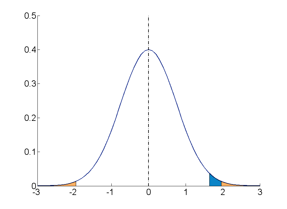
Suppose the rejection region is a single interval, so we need to select a single number \(C\). Here is the procedure for doing so. We select a small probability, denoted \(\alpha\), say \(1\%\), which we take as our definition of “rare event:” an event is “rare” if its probability of occurrence is less than \(\alpha\). (In all the examples and problems in this text the value of \(\alpha\) will be given already.) The probability that \(\overline{X}\) takes a value in an interval is the area under its density curve and above that interval, so as shown in Figure \(\PageIndex{2}\) (drawn under the assumption that \(H_0\) is true, so that the curve centers at \(\mu _0\)) the critical value \(C\) is the value of \(\overline{X}\) that cuts off a tail area \(\alpha\) in the probability density curve of \(\overline{X}\). When the rejection region is in two pieces, that is, composed of two intervals, the total area above both of them must be \(\alpha\), so the area above each one is \(\alpha /2\), as also shown in Figure \(\PageIndex{2}\).

The number \(\alpha\) is the total area of a tail or a pair of tails.

Example \(\PageIndex{3}\)

In the context of Example \(\PageIndex{2}\), suppose that it is known that the population is normally distributed with standard deviation \(\alpha =0.15\) gram, and suppose that the test of hypotheses \(H_0:\mu =8.0\) versus \(H_a:\mu \neq 8.0\) will be performed with a sample of size \(5\). Construct the rejection region for the test for the choice \(\alpha =0.10\). Explain the decision procedure and interpret it.

If \(H_0\) is true then the sample mean \(\overline{X}\) is normally distributed with mean and standard deviation

\[\begin{align} \mu _{\overline{X}} &=\mu \nonumber \\[5pt] &=8.0 \nonumber \end{align} \nonumber \]

\[\begin{align} \sigma _{\overline{X}}&=\dfrac{\sigma}{\sqrt{n}} \nonumber \\[5pt] &= \dfrac{0.15}{\sqrt{5}} \nonumber\\[5pt] &=0.067 \nonumber \end{align} \nonumber \]

Since \(H_a\) contains the \(\neq\) symbol the rejection region will be in two pieces, each one corresponding to a tail of area \(\alpha /2=0.10/2=0.05\). From Figure 7.1.6, \(z_{0.05}=1.645\), so \(C\) and \(C′\) are \(1.645\) standard deviations of \(\overline{X}\) to the right and left of its mean \(8.0\):

\[C=8.0-(1.645)(0.067) = 7.89 \; \; \text{and}\; \; C'=8.0 + (1.645)(0.067) = 8.11 \nonumber \]

The result is shown in Figure \(\PageIndex{3}\). α = 0.1

The decision procedure is: take a sample of size \(5\) and compute the sample mean \(\bar{x}\). If \(\bar{x}\) is either \(7.89\) grams or less or \(8.11\) grams or more then reject the hypothesis that the average amount of fat in all servings of the product is \(8.0\) grams in favor of the alternative that it is different from \(8.0\) grams. Otherwise do not reject the hypothesis that the average amount is \(8.0\) grams.

The reasoning is that if the true average amount of fat per serving were \(8.0\) grams then there would be less than a \(10\%\) chance that a sample of size \(5\) would produce a mean of either \(7.89\) grams or less or \(8.11\) grams or more. Hence if that happened it would be more likely that the value \(8.0\) is incorrect (always assuming that the population standard deviation is \(0.15\) gram).

Because the rejection regions are computed based on areas in tails of distributions, as shown in Figure \(\PageIndex{2}\), hypothesis tests are classified according to the form of the alternative hypothesis in the following way.

Definitions: Test classifications

• If \(H_a\) has the form \(\mu \neq \mu _0\) the test is called a two-tailed test .
• If \(H_a\) has the form \(\mu < \mu _0\) the test is called a left-tailed test .
• If \(H_a\) has the form \(\mu > \mu _0\)the test is called a right-tailed test .

Each of the last two forms is also called a one-tailed test .

Two Types of Errors

The format of the testing procedure in general terms is to take a sample and use the information it contains to come to a decision about the two hypotheses. As stated before our decision will always be either

• reject the null hypothesis \(H_0\) in favor of the alternative \(H_a\) presented, or
• do not reject the null hypothesis \(H_0\) in favor of the alternative \(H_0\) presented.

There are four possible outcomes of hypothesis testing procedure, as shown in the following table:

As the table shows, there are two ways to be right and two ways to be wrong. Typically to reject \(H_0\) when it is actually true is a more serious error than to fail to reject it when it is false, so the former error is labeled “ Type I ” and the latter error “ Type II ”.

Definition: Type I and Type II errors

In a test of hypotheses:

• A Type I error is the decision to reject \(H_0\) when it is in fact true.
• A Type II error is the decision not to reject \(H_0\) when it is in fact not true.

Unless we perform a census we do not have certain knowledge, so we do not know whether our decision matches the true state of nature or if we have made an error. We reject \(H_0\) if what we observe would be a “rare” event if \(H_0\) were true. But rare events are not impossible: they occur with probability \(\alpha\). Thus when \(H_0\) is true, a rare event will be observed in the proportion \(\alpha\) of repeated similar tests, and \(H_0\) will be erroneously rejected in those tests. Thus \(\alpha\) is the probability that in following the testing procedure to decide between \(H_0\) and \(H_a\) we will make a Type I error.

Definition: level of significance

The number \(\alpha\) that is used to determine the rejection region is called the level of significance of the test. It is the probability that the test procedure will result in a Type I error .

The probability of making a Type II error is too complicated to discuss in a beginning text, so we will say no more about it than this: for a fixed sample size, choosing \(alpha\) smaller in order to reduce the chance of making a Type I error has the effect of increasing the chance of making a Type II error . The only way to simultaneously reduce the chances of making either kind of error is to increase the sample size.

Standardizing the Test Statistic

Hypotheses testing will be considered in a number of contexts, and great unification as well as simplification results when the relevant sample statistic is standardized by subtracting its mean from it and then dividing by its standard deviation. The resulting statistic is called a standardized test statistic . In every situation treated in this and the following two chapters the standardized test statistic will have either the standard normal distribution or Student’s \(t\)-distribution.

Definition: hypothesis test

A standardized test statistic for a hypothesis test is the statistic that is formed by subtracting from the statistic of interest its mean and dividing by its standard deviation.

For example, reviewing Example \(\PageIndex{3}\), if instead of working with the sample mean \(\overline{X}\) we instead work with the test statistic

\[\frac{\overline{X}-8.0}{0.067} \nonumber \]

then the distribution involved is standard normal and the critical values are just \(\pm z_{0.05}\). The extra work that was done to find that \(C=7.89\) and \(C′=8.11\) is eliminated. In every hypothesis test in this book the standardized test statistic will be governed by either the standard normal distribution or Student’s \(t\)-distribution. Information about rejection regions is summarized in the following tables:

Every instance of hypothesis testing discussed in this and the following two chapters will have a rejection region like one of the six forms tabulated in the tables above.

No matter what the context a test of hypotheses can always be performed by applying the following systematic procedure, which will be illustrated in the examples in the succeeding sections.

Systematic Hypothesis Testing Procedure: Critical Value Approach

• Identify the null and alternative hypotheses.
• Identify the relevant test statistic and its distribution.
• Compute from the data the value of the test statistic.
• Construct the rejection region.
• Compare the value computed in Step 3 to the rejection region constructed in Step 4 and make a decision. Formulate the decision in the context of the problem, if applicable.

The procedure that we have outlined in this section is called the “Critical Value Approach” to hypothesis testing to distinguish it from an alternative but equivalent approach that will be introduced at the end of Section 8.3.

Key Takeaway

• A test of hypotheses is a statistical process for deciding between two competing assertions about a population parameter.
• The testing procedure is formalized in a five-step procedure.

Hypothesis test

A significance test, also referred to as a statistical hypothesis test, is a method of statistical inference in which observed data is compared to a claim (referred to as a hypothesis) in order to assess the truth of the claim. For example, one might wonder whether age affects the number of apples a person can eat, and may use a significance test to determine whether there is any evidence to suggest that it does.

Generally, the process of statistical hypothesis testing involves the following steps:

• State the null hypothesis.
• State the alternative hypothesis.
• Select the appropriate test statistic and select a significance level.
• Compute the observed value of the test statistic and its corresponding p-value.
• Reject the null hypothesis in favor of the alternative hypothesis, or do not reject the null hypothesis.

The null hypothesis

The null hypothesis, H 0 , is the claim that is being tested in a statistical hypothesis test. It typically is a statement that there is no difference between the populations being studied, or that there is no evidence to support a claim being made. For example, "age has no effect on the number of apples a person can eat."

A significance test is designed to test the evidence against the null hypothesis. This is because it is easier to prove that a claim is false than to prove that it is true; demonstrating that the claim is false in one case is sufficient, while proving that it is true requires that the claim be true in all cases.

The alternative hypothesis

The alternative hypothesis is the opposite of the null hypothesis in that it is a statement that there is some difference between the populations being studied. For example, "younger people can eat more apples than older people."

The alternative hypothesis is typically the hypothesis that researchers are trying to prove. A significance test is meant to determine whether there is sufficient evidence to reject the null hypothesis in favor of the alternative hypothesis. Note that the results of a significance test should either be to reject the null hypothesis in favor of the alternative hypothesis, or to not reject the null hypothesis. The result should not be to reject the alternative hypothesis or to accept the alternative hypothesis.

Test statistics and significance level

A test statistic is a statistic that is calculated as part of hypothesis testing that compares the distribution of observed data to the expected distribution, based on the null hypothesis. Examples of test statistics include the Z-score, T-statistic, F-statistic, and the Chi-square statistic. The test statistic used is dependent on the significance test used, which is dependent on the type of data collected and the type of relationship to be tested.

In many cases, the chosen significance level is 0.05, though 0.01 is also used. A significance level of 0.05 indicates that there is a 5% chance of rejecting the null hypothesis when the null hypothesis is actually true. Thus, a smaller selected significance level will require more evidence if the null hypothesis is to be rejected in favor of the alternative hypothesis.

After the test statistic is computed, the p-value can be determined based on the result of the test statistic. The p-value indicates the probability of obtaining test results that are at least as extreme as the observed results, under the assumption that the null hypothesis is correct. It tells us how likely it is to obtain a result based solely on chance. The smaller the p-value, the less likely a result can occur purely by chance, while a larger p-value makes it more likely. For example, a p-value of 0.01 means that there is a 1% chance that a result occurred solely by chance, given that the null hypothesis is true; a p-value of 0.90 means that there is a 90% chance.

A p-value is significantly affected by sample size. The larger the sample size, the smaller the p-value, even if the difference between populations may not be meaningful. On the other hand, if a sample size is too small, a meaningful difference may not be detected.

The last step in a significance test is to determine whether the p-value provides evidence that the null hypothesis should be rejected in favor of the alternative hypothesis. This is based on the selected significance level. If the p-value is less than or equal to the selected significance level, the null hypothesis is rejected in favor of the alternative hypothesis, and the result is deemed statistically significant. If the p-value is greater than the selected significance level, the null hypothesis is not rejected, and the result is deemed not statistically significant.

Forgot password? New user? Sign up

Existing user? Log in

Hypothesis Testing

Already have an account? Log in here.

A hypothesis test is a statistical inference method used to test the significance of a proposed (hypothesized) relation between population statistics (parameters) and their corresponding sample estimators . In other words, hypothesis tests are used to determine if there is enough evidence in a sample to prove a hypothesis true for the entire population.

The test considers two hypotheses: the null hypothesis , which is a statement meant to be tested, usually something like "there is no effect" with the intention of proving this false, and the alternate hypothesis , which is the statement meant to stand after the test is performed. The two hypotheses must be mutually exclusive ; moreover, in most applications, the two are complementary (one being the negation of the other). The test works by comparing the \(p\)-value to the level of significance (a chosen target). If the \(p\)-value is less than or equal to the level of significance, then the null hypothesis is rejected.

When analyzing data, only samples of a certain size might be manageable as efficient computations. In some situations the error terms follow a continuous or infinite distribution, hence the use of samples to suggest accuracy of the chosen test statistics. The method of hypothesis testing gives an advantage over guessing what distribution or which parameters the data follows.

Definitions and Methodology

Hypothesis test and confidence intervals.

In statistical inference, properties (parameters) of a population are analyzed by sampling data sets. Given assumptions on the distribution, i.e. a statistical model of the data, certain hypotheses can be deduced from the known behavior of the model. These hypotheses must be tested against sampled data from the population.

The null hypothesis \((\)denoted \(H_0)\) is a statement that is assumed to be true. If the null hypothesis is rejected, then there is enough evidence (statistical significance) to accept the alternate hypothesis \((\)denoted \(H_1).\) Before doing any test for significance, both hypotheses must be clearly stated and non-conflictive, i.e. mutually exclusive, statements. Rejecting the null hypothesis, given that it is true, is called a type I error and it is denoted \(\alpha\), which is also its probability of occurrence. Failing to reject the null hypothesis, given that it is false, is called a type II error and it is denoted \(\beta\), which is also its probability of occurrence. Also, \(\alpha\) is known as the significance level , and \(1-\beta\) is known as the power of the test. \(H_0\) \(\textbf{is true}\)\(\hspace{15mm}\) \(H_0\) \(\textbf{is false}\) \(\textbf{Reject}\) \(H_0\)\(\hspace{10mm}\) Type I error Correct Decision \(\textbf{Reject}\) \(H_1\) Correct Decision Type II error The test statistic is the standardized value following the sampled data under the assumption that the null hypothesis is true, and a chosen particular test. These tests depend on the statistic to be studied and the assumed distribution it follows, e.g. the population mean following a normal distribution. The \(p\)-value is the probability of observing an extreme test statistic in the direction of the alternate hypothesis, given that the null hypothesis is true. The critical value is the value of the assumed distribution of the test statistic such that the probability of making a type I error is small.

Methodologies: Given an estimator \(\hat \theta\) of a population statistic \(\theta\), following a probability distribution \(P(T)\), computed from a sample \(\mathcal{S},\) and given a significance level \(\alpha\) and test statistic \(t^*,\) define \(H_0\) and \(H_1;\) compute the test statistic \(t^*.\) \(p\)-value Approach (most prevalent): Find the \(p\)-value using \(t^*\) (right-tailed). If the \(p\)-value is at most \(\alpha,\) reject \(H_0\). Otherwise, reject \(H_1\). Critical Value Approach: Find the critical value solving the equation \(P(T\geq t_\alpha)=\alpha\) (right-tailed). If \(t^*>t_\alpha\), reject \(H_0\). Otherwise, reject \(H_1\). Note: Failing to reject \(H_0\) only means inability to accept \(H_1\), and it does not mean to accept \(H_0\).

Assume a normally distributed population has recorded cholesterol levels with various statistics computed. From a sample of 100 subjects in the population, the sample mean was 214.12 mg/dL (milligrams per deciliter), with a sample standard deviation of 45.71 mg/dL. Perform a hypothesis test, with significance level 0.05, to test if there is enough evidence to conclude that the population mean is larger than 200 mg/dL. Hypothesis Test We will perform a hypothesis test using the \(p\)-value approach with significance level \(\alpha=0.05:\) Define \(H_0\): \(\mu=200\). Define \(H_1\): \(\mu>200\). Since our values are normally distributed, the test statistic is \(z^*=\frac{\bar X - \mu_0}{\frac{s}{\sqrt{n}}}=\frac{214.12 - 200}{\frac{45.71}{\sqrt{100}}}\approx 3.09\). Using a standard normal distribution, we find that our \(p\)-value is approximately \(0.001\). Since the \(p\)-value is at most \(\alpha=0.05,\) we reject \(H_0\). Therefore, we can conclude that the test shows sufficient evidence to support the claim that \(\mu\) is larger than \(200\) mg/dL.

If the sample size was smaller, the normal and \(t\)-distributions behave differently. Also, the question itself must be managed by a double-tail test instead.

Assume a population's cholesterol levels are recorded and various statistics are computed. From a sample of 25 subjects, the sample mean was 214.12 mg/dL (milligrams per deciliter), with a sample standard deviation of 45.71 mg/dL. Perform a hypothesis test, with significance level 0.05, to test if there is enough evidence to conclude that the population mean is not equal to 200 mg/dL. Hypothesis Test We will perform a hypothesis test using the \(p\)-value approach with significance level \(\alpha=0.05\) and the \(t\)-distribution with 24 degrees of freedom: Define \(H_0\): \(\mu=200\). Define \(H_1\): \(\mu\neq 200\). Using the \(t\)-distribution, the test statistic is \(t^*=\frac{\bar X - \mu_0}{\frac{s}{\sqrt{n}}}=\frac{214.12 - 200}{\frac{45.71}{\sqrt{25}}}\approx 1.54\). Using a \(t\)-distribution with 24 degrees of freedom, we find that our \(p\)-value is approximately \(2(0.068)=0.136\). We have multiplied by two since this is a two-tailed argument, i.e. the mean can be smaller than or larger than. Since the \(p\)-value is larger than \(\alpha=0.05,\) we fail to reject \(H_0\). Therefore, the test does not show sufficient evidence to support the claim that \(\mu\) is not equal to \(200\) mg/dL.

The complement of the rejection on a two-tailed hypothesis test (with significance level \(\alpha\)) for a population parameter \(\theta\) is equivalent to finding a confidence interval \((\)with confidence level \(1-\alpha)\) for the population parameter \(\theta\). If the assumption on the parameter \(\theta\) falls inside the confidence interval, then the test has failed to reject the null hypothesis \((\)with \(p\)-value greater than \(\alpha).\) Otherwise, if \(\theta\) does not fall in the confidence interval, then the null hypothesis is rejected in favor of the alternate \((\)with \(p\)-value at most \(\alpha).\)

• Statistics (Estimation)
• Normal Distribution
• Correlation
• Confidence Intervals

Problem Loading...

Note Loading...

Set Loading...

Want to create or adapt books like this? Learn more about how Pressbooks supports open publishing practices.

17 Introduction to Hypothesis Testing

Jenna Lehmann

What is Hypothesis Testing?

Hypothesis testing is a big part of what we would actually consider testing for inferential statistics. It’s a procedure and set of rules that allow us to move from descriptive statistics to make inferences about a population based on sample data. It is a statistical method that uses sample data to evaluate a hypothesis about a population.

This type of test is usually used within the context of research. If we expect to see a difference between a treated and untreated group (in some cases the untreated group is the parameters we know about the population), we expect there to be a difference in the means between the two groups, but that the standard deviation remains the same, as if each individual score has had a value added or subtracted from it.

Steps of Hypothesis Testing

The following steps will be tailored to fit the first kind of hypothesis testing we will learn first: single-sample z-tests. There are many other kinds of tests, so keep this in mind.

• Null Hypothesis (H0): states that in the general population there is no change, no difference, or no relationship, or in the context of an experiment, it predicts that the independent variable has no effect on the dependent variable.
• Alternative Hypothesis (H1): states that there is a change, a difference, or a relationship for the general population, or in the context of an experiment, it predicts that the independent variable has an effect on the dependent variable.

• Critical Region: Composed of the extreme sample values that are very unlikely to be obtained if the null hypothesis is true. Determined by alpha level. If sample data fall in the critical region, the null hypothesis is rejected, because it’s very unlikely they’ve fallen there by chance.
• After collecting the data, we find the sample mean. Now we can compare the sample mean with the null hypothesis by computing a z-score that describes where the sample mean is located relative to the hypothesized population mean. We use the z-score formula.
• We decided previously what the two z-score boundaries are for a critical score. If the z-score we get after plugging the numbers in the aforementioned equation is outside of that critical region, we reject the null hypothesis. Otherwise, we would say that we failed to reject the null hypothesis.

Regions of the Distribution

Because we’re making judgments based on probability and proportion, our normal distributions and certain regions within them come into play.

The Critical Region is composed of the extreme sample values that are very unlikely to be obtained if the null hypothesis is true. Determined by alpha level. If sample data fall in the critical region, the null hypothesis is rejected, because it’s very unlikely they’ve fallen there by chance.

These regions come into play when talking about different errors.

A Type I Error occurs when a researcher rejects a null hypothesis that is actually true; the researcher concludes that a treatment has an effect when it actually doesn’t. This happens when a researcher unknowingly obtains an extreme, non-representative sample. This goes back to alpha level: it’s the probability that the test will lead to a Type I error if the null hypothesis is true.

A result is said to be significant or statistically significant if it is very unlikely to occur when the null hypothesis is true. That is, the result is sufficient to reject the null hypothesis. For instance, two means can be significantly different from one another.

Factors that Influence and Assumptions of Hypothesis Testing

Assumptions of Hypothesis Testing:

• Random sampling: it is assumed that the participants used in the study were selected randomly so that we can confidently generalize our findings from the sample to the population.
• Independent observation: two observations are independent if there is no consistent, predictable relationship between the first observation and the second. The value of σ is unchanged by the treatment; if the population standard deviation is unknown, we assume that the standard deviation for the unknown population (after treatment) is the same as it was for the population before treatment. There are ways of checking to see if this is true in SPSS or Excel.
• Normal sampling distribution: in order to use the unit normal table to identify the critical region, we need the distribution of sample means to be normal (which means we need the population to be distributed normally and/or each sample size needs to be 30 or greater based on what we know about the central limit theorem).

Factors that influence hypothesis testing:

• The variability of the scores, which is measured by either the standard deviation or the variance. The variability influences the size of the standard error in the denominator of the z-score.
• The number of scores in the sample. This value also influences the size of the standard error in the denominator.

Test statistic: indicates that the sample data are converted into a single, specific statistic that is used to test the hypothesis (in this case, the z-score statistic).

Directional Hypotheses and Tailed Tests

In a directional hypothesis test , also known as a one-tailed test, the statistical hypotheses specify with an increase or decrease in the population mean. That is, they make a statement about the direction of the effect.

The Hypotheses for a Directional Test:

• H0: The test scores are not increased/decreased (the treatment doesn’t work)
• H1: The test scores are increased/decreased (the treatment works as predicted)

Because we’re only worried about scores that are either greater or less than the scores predicted by the null hypothesis, we only worry about what’s going on in one tail meaning that the critical region only exists within one tail. This means that all of the alpha is contained in one tail rather than split up into both (so the whole 5% is located in the tail we care about, rather than 2.5% in each tail). So before, we cared about what’s going on at the 0.025 mark of the unit normal table to look at both tails, but now we care about 0.05 because we’re only looking at one tail.

A one-tailed test allows you to reject the null hypothesis when the difference between the sample and the population is relatively small, as long as that difference is in the direction that you predicted. A two-tailed test, on the other hand, requires a relatively large difference independent of direction. In practice, researchers hypothesize using a one-tailed method but base their findings off of whether the results fall into the critical region of a two-tailed method. For the purposes of this class, make sure to calculate your results using the test that is specified in the problem.

Effect Size

A measure of effect size is intended to provide a measurement of the absolute magnitude of a treatment effect, independent of the size of the sample(s) being used. Usually done with Cohen’s d. If you imagine the two distributions, they’re layered over one another. The more they overlap, the smaller the effect size (the means of the two distributions are close). The more they are spread apart, the greater the effect size (the means of the two distributions are farther apart).

Statistical Power

The power of a statistical test is the probability that the test will correctly reject a false null hypothesis. It’s usually what we’re hoping to get when we run an experiment. It’s displayed in the table posted above. Power and effect size are connected. So, we know that the greater the distance between the means, the greater the effect size. If the two distributions overlapped very little, there would be a greater chance of selecting a sample that leads to rejecting the null hypothesis.

This chapter was originally posted to the Math Support Center blog at the University of Baltimore on June 11, 2019.

Math and Statistics Guides from UB's Math & Statistics Center Copyright © by Jenna Lehmann is licensed under a Creative Commons Attribution-NonCommercial-ShareAlike 4.0 International License , except where otherwise noted.

Share This Book

• Hypothesis testing

by Marco Taboga , PhD

Hypothesis testing is a method of making statistical inferences in which:

we establish an hypothesis, called null hypothesis;

we use some data to decide whether to reject or not to reject the hypothesis.

This lecture provides a rigorous introduction to the mathematics of hypothesis tests, and it provides several links to other pages where the single steps of a test of hypothesis can be studied in more detail.

Table of contents

What you need to know to get started

Testing restrictions, parametric tests, null hypothesis.

• Alternative hypothesis

Types of errors

Critical region, test statistic, power function, size of a test, criteria to evaluate tests.

Remember that a statistical inference is a statement about the probability distribution from which a sample has been drawn.

The statement we make is chosen between two possible statements:

For concreteness, we will focus on parametric hypothesis testing in this lecture, but most of the things we will say apply with straightforward modifications to hypothesis testing in general.

Understanding how to formulate a null hypothesis is a fundamental step in hypothesis testing. We suggest to read a thorough discussion of null hypotheses here .

When we decide whether to reject a restriction or not to reject it, we can incur in two types of errors:

This mathematical formulation is made more concrete in the next section.

The critical region is often implicitly defined in terms of a test statistic and a critical region for the test statistic.

Example In our example, where we are testing that the mean of the normal distribution is zero, we could use a test statistic called z-statistic. If you want to read the details, go to the lecture on hypothesis tests about the mean .

This maximum probability is called the size of the test .

The size of the test is also called by some authors the level of significance of the test. However, according to other authors, who assign a slightly different meaning to the term, the level of significance of a test is an upper bound on the size of the test.

Tests of hypothesis are most commonly evaluated based on their size and power.

An ideal test should have:

Of course, such an ideal test is never found in practice, but the best we can hope for is a test with a very small size and a very high probability of rejecting a false hypothesis. Nevertheless, this ideal is routinely used to choose among different tests.

For example:

Several other criteria, beyond power and size, are used to evaluate tests of hypothesis. We do not discuss them here, but we refer the reader to the very nice exposition in Berger and Casella (2002).

Examples of how the mathematics of hypothesis testing works can be found in the following lectures:

Hypothesis tests about the mean (examples of tests of hypothesis about the mean of an unknown distribution);

Hypothesis tests about the variance (examples of tests of hypothesis about the variance of an unknown distribution).

Berger, R. L. and G. Casella (2002) "Statistical inference", Duxbury Advanced Series.

How to cite

Please cite as:

Taboga, Marco (2021). "Hypothesis testing", Lectures on probability theory and mathematical statistics. Kindle Direct Publishing. Online appendix. https://www.statlect.com/fundamentals-of-statistics/hypothesis-testing.

Most of the learning materials found on this website are now available in a traditional textbook format.

• Central Limit Theorem
• Beta distribution
• F distribution
• Point estimation
• Bernoulli distribution
• Likelihood ratio test
• Multinomial distribution
• Mathematical tools
• Fundamentals of probability
• Probability distributions
• Asymptotic theory
• Fundamentals of statistics
• About Statlect
• Cookies, privacy and terms of use
• Critical value
• Almost sure
• Continuous random variable
• Probability density function
• Integrable variable
• To enhance your privacy,
• we removed the social buttons,
• but don't forget to share .

Hypothesis testing

When interpreting research findings, researchers need to assess whether these findings may have occurred by chance. Hypothesis testing is a systematic procedure for deciding whether the results of a research study support a particular theory which applies to a population.

Hypothesis testing uses sample data to evaluate a hypothesis about a population . A hypothesis test assesses how unusual the result is, whether it is reasonable chance variation or whether the result is too extreme to be considered chance variation.

Basic concepts

• Null and research hypothesis

Probability value and types of errors

Effect size and statistical significance.

• Directional and non-directional hypotheses

Null and research hypotheses

To carry out statistical hypothesis testing, research and null hypothesis are employed:

• Research hypothesis : this is the hypothesis that you propose, also known as the alternative hypothesis HA. For example:

H A: There is a relationship between intelligence and academic results.

H A: First year university students obtain higher grades after an intensive Statistics course.

H A; Males and females differ in their levels of stress.

• The null hypothesis (H o ) is the opposite of the research hypothesis and expresses that there is no relationship between variables, or no differences between groups; for example:

H o : There is no relationship between intelligence and academic results.

H o:  First year university students do not obtain higher grades after an intensive Statistics course.

H o : Males and females will not differ in their levels of stress.

The purpose of hypothesis testing is to test whether the null hypothesis (there is no difference, no effect) can be rejected or approved. If the null hypothesis is rejected, then the research hypothesis can be accepted. If the null hypothesis is accepted, then the research hypothesis is rejected.

In hypothesis testing, a value is set to assess whether the null hypothesis is accepted or rejected and whether the result is statistically significant:

• A critical value is the score the sample would need to decide against the null hypothesis.
• A probability value is used to assess the significance of the statistical test. If the null hypothesis is rejected, then the alternative to the null hypothesis is accepted.

The probability value, or p value , is the probability of an outcome or research result given the hypothesis. Usually, the probability value is set at 0.05: the null hypothesis will be rejected if the probability value of the statistical test is less than 0.05. There are two types of errors associated to hypothesis testing:

• What if we observe a difference – but none exists in the population?
• What if we do not find a difference – but it does exist in the population?

These situations are known as Type I and Type II errors:

• Type I Error: is the type of error that involves the rejection of a null hypothesis that is actually true (i.e. a false positive).
• Type II Error:  is the type of error that occurs when we do not reject a null hypothesis that is false (i.e. a false negative).

These errors cannot be eliminated; they can be minimised, but minimising one type of error will increase the probability of committing the other type.

The probability of making a Type I error depends on the criterion that is used to accept or reject the null hypothesis: the p value or alpha level . The alpha is set by the researcher, usually at .05, and is the chance the researcher is willing to take and still claim the significance of the statistical test.). Choosing a smaller alpha level will decrease the likelihood of committing Type I error.

For example, p<0.05  indicates that there are 5 chances in 100 that the difference observed was really due to sampling error – that 5% of the time a Type I error will occur or that there is a 5% chance that the opposite of the null hypothesis is actually true.

With a p<0.01, there will be 1 chance in 100 that the difference observed was really due to sampling error – 1% of the time a Type I error will occur.

The p level is specified before analysing the data. If the data analysis results in a probability value below the α (alpha) level, then the null hypothesis is rejected; if it is not, then the null hypothesis is not rejected.

When the null hypothesis is rejected, the effect is said to be statistically significant. However, statistical significance does not mean that the effect is important.

A result can be statistically significant, but the effect size may be small. Finding that an effect is significant does not provide information about how large or important the effect is. In fact, a small effect can be statistically significant if the sample size is large enough.

Information about the effect size, or magnitude of the result, is given by the statistical test. For example, the strength of the correlation between two variables is given by the coefficient of correlation, which varies from 0 to 1.

• A hypothesis that states that students who attend an intensive Statistics course will obtain higher grades than students who do not attend would be directional.
• A non-directional hypothesis states that there will be differences between students who attend do or don’t attend an intensive Statistics course, but we don’t know what group will get higher grades than the other. The hypothesis only states that they will obtain different grades.

The hypothesis testing process

The hypothesis testing process can be divided into five steps:

• Restate the research question as research hypothesis and a null hypothesis about the populations.
• Determine the characteristics of the comparison distribution.
• Determine the cut off sample score on the comparison distribution at which the null hypothesis should be rejected.
• Determine your sample’s score on the comparison distribution.
• Decide whether to reject the null hypothesis.

This example illustrates how these five steps can be applied to text a hypothesis:

• Let’s say that you conduct an experiment to investigate whether students’ ability to memorise words improves after they have consumed caffeine.
• The experiment involves two groups of students: the first group consumes caffeine; the second group drinks water.
• Both groups complete a memory test.
• A randomly selected individual in the experimental condition (i.e. the group that consumes caffeine) has a score of 27 on the memory test. The scores of people in general on this memory measure are normally distributed with a mean of 19 and a standard deviation of 4.
• The researcher predicts an effect (differences in memory for these groups) but does not predict a particular direction of effect (i.e. which group will have higher scores on the memory test). Using the 5% significance level, what should you conclude?

Step 1 : There are two populations of interest.

Population 1: People who go through the experimental procedure (drink coffee).

Population 2: People who do not go through the experimental procedure (drink water).

• Research hypothesis: Population 1 will score differently from Population 2.
• Null hypothesis: There will be no difference between the two populations.

Step 2 : We know that the characteristics of the comparison distribution (student population) are:

Population M = 19, Population SD= 4, normally distributed. These are the mean and standard deviation of the distribution of scores on the memory test for the general student population.

Step 3 : For a two-tailed test (the direction of the effect is not specified) at the 5% level (25% at each tail), the cut off sample scores are +1.96 and -1.99.

Step 4 : Your sample score of 27 needs to be converted into a Z value. To calculate Z = (27-19)/4= 2 ( check the Converting into Z scores section if you need to review how to do this process)

Step 5 : A ‘Z’ score of 2 is more extreme than the cut off Z of +1.96 (see figure above). The result is significant and, thus, the null hypothesis is rejected.

You can find more examples here:

• Statistics (RMIT Learning Lab)

Some commonly used statistical techniques

Correlation analysis, multiple regression.

• Analysis of variance

Chi-square test for independence

Correlation analysis explores the association between variables . The purpose of correlational analysis is to discover whether there is a relationship between variables, which is unlikely to occur by sampling error. The null hypothesis is that there is no relationship between the two variables. Correlation analysis provides information about:

• The direction of the relationship: positive or negative- given by the sign of the correlation coefficient.
• The strength or magnitude of the relationship between the two variables- given by the correlation coefficient, which varies from 0 (no relationship between the variables) to 1 (perfect relationship between the variables).
• Direction of the relationship.

A positive correlation indicates that high scores on one variable are associated with high scores on the other variable; low scores on one variable are associated with low scores on the second variable . For instance, in the figure below, higher scores on negative affect are associated with higher scores on perceived stress

A negative correlation indicates that high scores on one variable are associated with low scores on the other variable. The graph shows that a person who scores high on perceived stress will probably score low on mastery. The slope of the graph is downwards- as it moves to the right. In the figure below, higher scores on mastery are associated with lower scores on perceived stress.

Fig 2. Negative correlation between two variables. Adapted from Pallant, J. (2013). SPSS survival manual: A step by step guide to data analysis using IBM SPSS (5th ed.). Sydney, Melbourne, Auckland, London: Allen & Unwin

2. The strength or magnitude of the relationship

The strength of a linear relationship between two variables is measured by a statistic known as the correlation coefficient , which varies from 0 to -1, and from 0 to +1. There are several correlation coefficients; the most widely used are Pearson’s r and Spearman’s rho. The strength of the relationship is interpreted as follows:

• Small/weak: r= .10 to .29
• Medium/moderate: r= .30 to .49
• Large/strong: r= .50 to 1

It is important to note that correlation analysis does not imply causality. Correlation is used to explore the association between variables, however, it does not indicate that one variable causes the other. The correlation between two variables could be due to the fact that a third variable is affecting the two variables.

Multiple regression is an extension of correlation analysis. Multiple regression is used to explore the relationship between one dependent variable and a number of independent variables or predictors . The purpose of a multiple regression model is to predict values of a dependent variable based on the values of the independent variables or predictors. For example, a researcher may be interested in predicting students’ academic success (e.g. grades) based on a number of predictors, for example, hours spent studying, satisfaction with studies, relationships with peers and lecturers.

A multiple regression model can be conducted using statistical software (e.g. SPSS). The software will test the significance of the model (i.e. does the model significantly predicts scores on the dependent variable using the independent variables introduced in the model?), how much of the variance in the dependent variable is explained by the model, and the individual contribution of each independent variable.

Example of multiple regression model

From Dunn et al. (2014). Influence of academic self-regulation, critical thinking, and age on online graduate students' academic help-seeking.

In this model, help-seeking is the dependent variable; there are three independent variables or predictors. The coefficients show the direction (positive or negative) and magnitude of the relationship between each predictor and the dependent variable. The model was statistically significant and predicted 13.5% of the variance in help-seeking.

t-Tests are employed to compare the mean score on some continuous variable for two groups . The null hypothesis to be tested is there are no differences between the two groups (e.g. anxiety scores for males and females are not different).

If the significance value of the t-test is equal or less than .05, there is a significant difference in the mean scores on the variable of interest for each of the two groups. If the value is above .05, there is no significant difference between the groups.

t-Tests can be employed to compare the mean scores of two different groups (independent-samples t-test ) or to compare the same group of people on two different occasions ( paired-samples t-test) .

In addition to assessing whether the difference between the two groups is statistically significant, it is important to consider the effect size or magnitude of the difference between the groups. The effect size is given by partial eta squared (proportion of variance of the dependent variable that is explained by the independent variable) and Cohen’s d (difference between groups in terms of standard deviation units).

In this example, an independent samples t-test was conducted to assess whether males and females differ in their perceived anxiety levels. The significance of the test is .004. Since this value is less than .05, we can conclude that there is a statistically significant difference between males and females in their perceived anxiety levels.

Whilst t-tests compare the mean score on one variable for two groups, analysis of variance is used to test more than two groups . Following the previous example, analysis of variance would be employed to test whether there are differences in anxiety scores for students from different disciplines.

Analysis of variance compare the variance (variability in scores) between the different groups (believed to be due to the independent variable) with the variability within each group (believed to be due to chance). An F ratio is calculated; a large F ratio indicates that there is more variability between the groups (caused by the independent variable) than there is within each group (error term). A significant F test indicates that we can reject the null hypothesis; i.e. that there is no difference between the groups.

Again, effect size statistics such as Cohen’s d and eta squared are employed to assess the magnitude of the differences between groups.

In this example, we examined differences in perceived anxiety between students from different disciplines. The results of the Anova Test show that the significance level is .005. Since this value is below .05, we can conclude that there are statistically significant differences between students from different disciplines in their perceived anxiety levels.

Chi-square test for independence is used to explore the relationship between two categorical variables. Each variable can have two or more categories.

For example, a researcher can use a Chi-square test for independence to assess the relationship between study disciplines (e.g. Psychology, Business, Education,…) and help-seeking behaviour (Yes/No). The test compares the observed frequencies of cases with the values that would be expected if there was no association between the two variables of interest. A statistically significant Chi-square test indicates that the two variables are associated (e.g. Psychology students are more likely to seek help than Business students). The effect size is assessed using effect size statistics: Phi and Cramer’s V .

In this example, a Chi-square test was conducted to assess whether males and females differ in their help-seeking behaviour (Yes/No). The crosstabulation table shows the percentage of males of females who sought/didn't seek help. The table 'Chi square tests' shows the significance of the test (Pearson Chi square asymp sig: .482). Since this value is above .05, we conclude that there is no statistically significant difference between males and females in their help-seeking behaviour.

• << Previous: Probability and the normal distribution
• Next: Statistical techniques >>

Or search by topic

Number and algebra

• The Number System and Place Value
• Calculations and Numerical Methods
• Fractions, Decimals, Percentages, Ratio and Proportion
• Properties of Numbers
• Patterns, Sequences and Structure
• Algebraic expressions, equations and formulae
• Coordinates, Functions and Graphs

Geometry and measure

• Angles, Polygons, and Geometrical Proof
• 3D Geometry, Shape and Space
• Measuring and calculating with units
• Transformations and constructions
• Pythagoras and Trigonometry
• Vectors and Matrices

Probability and statistics

• Handling, Processing and Representing Data
• Probability

Working mathematically

• Thinking mathematically
• Mathematical mindsets
• Cross-curricular contexts
• Physical and digital manipulatives

For younger learners

• Early Years Foundation Stage

Advanced mathematics

• Decision Mathematics and Combinatorics
• Advanced Probability and Statistics

Published 2018 Revised 2019

What Is a Hypothesis Test?

The null hypothesis significance testing (nhst) framework, our simple scenario.

• Our null hypothesis is $H_0\colon \pi=\frac{1}{2}$.  This says that the proportion is what we believe it should be.
• Our alternative hypothesis is $H_1\colon \pi\ne\frac{1}{2}$.  This says that the proportion has changed.

Testing our hypotheses

• We can work out the critical region for $X$, that is, those extreme values of $X$ which would lead us to reject the null hypothesis at 5% significance.  (This can be done even before performing the experiment.)  The probability of $X$ taking a value in this critical region, assuming that the null hypothesis is true, should be 5%, or as close at we can get to 5% without going over it.  In symbols, we can say: $$\mathrm{P}(\text{$X$ in critical region} | \text{$H_0$ is true}) \le 0.05.$$ Then we reject the null hypothesis if $X$ lies in that region.
• We can work out the probability of $X$ taking the value it did or a more extreme value, assuming that the null hypothesis is true.  This is known as the p-value .  If the p-value is less than 0.05, then we will reject the null hypothesis at 5% significance. [ note 1 ]  In symbols, we can write $$\text{p-value} = \mathrm{P}(\text{$X$ taking this or a more extreme value} | \text{$H_0$ is true}).$$

Other types of scenario

• Does this drug/treatment/intervention/... have any effect?
• Which of these drugs/... is more effective, or are they equally effective?
• Is the mean height/mass/intelligence/test score/... of this population equal to some predicted value?
• Is the standard deviation of the height/mass/... equal to some predicted value?
• For two distinct groups of people, is their mean height/mass/... of each group the same?
• Does this group of people's heights/masses/... appear to be following the probability distribution we expect?
• Do these two populations' heights/masses/... appear to have the same distribution as each other?
• Do this population's heights and weights appear to be correlated?

Interpreting the results

The key question that hypothesis testing (nhst) answers, what a hypothesis test does not tell us, a non-significant result.

• It could be that the null hypothesis is true.  In this case, we would have to be unlucky to get a significant p-value, so most of the time, we will end up accepting the null hypothesis.  (If the null hypothesis is true, we would reject it with a probability of only 0.05.)  
• On the other hand, it could be that the alternative hypothesis is true, but we did not use a large enough sample to obtain a significant result (or we were just unlucky).  In such a case, we could say that our test was insensitive .  In this situation (the alternative hypothesis is true but we do not reject the null hypothesis), we say that we have made a Type II error .  The probability of this happening depends on the sample size and on how different the true $\pi$ is from $\frac{1}{2}$ (or whatever our null hypothesis says), as is explored in Powerful Hypothesis Testing .

A significant result

• It could be that the null hypothesis is true.  In this case, we reject the null hypothesis with a probability of $0.05=\frac{1}{20}$, that is, one time in 20 (at a significance level of 5%), so we were just unlucky.  
• On the other hand, the alternative hypothesis could indeed be true.  Either the sample was large enough to obtain a significant result, or the sample size wasn't that large, but we were just lucky.

Using this tree diagram, we can work out the probabilities of $H_0$ being true or $H_1$ being true given our experimental results.  To avoid the expressions becoming unwieldy, we will write $H_0$ for "$\text{$H_0$ true}$", $H_1$ for "$\text{$H_1$ true}$" and "$\text{p}^+$" for "observed p-value or more extreme".  Then we can write (conditional) probabilities on the branches of the tree diagram leading to our observed p-value: [ note 2 ]

The two routes which give our observed p-value (or more extreme) have the following probabilities: $$\begin{align*} \mathrm{P}(H_0\cap \text{p}^+) &= \mathrm{P}(H_0) \times \mathrm{P}(\text{p}^+ | H_0) \\ \mathrm{P}(H_1\cap \text{p}^+) &= \mathrm{P}(H_1) \times \mathrm{P}(\text{p}^+ | H_1) \end{align*}$$ (Recall that $\mathrm{P}(H_0\cap \text{p}^+)$ means "the probability of $H_0$ being true and the p-value being that observed or more extreme".) We can therefore work out the probability of the alternative hypothesis being true given the observed p-value, using conditional probability: $$\begin{align*} \mathrm{P}(H_1|\text{p}^+) &= \frac{\mathrm{P}(H_1\cap \text{p}^+)}{\mathrm{P}(\text{p}^+)} \\ &= \frac{\mathrm{P}(H_1\cap \text{p}^+)}{\mathrm{P}(H_0\cap\text{p}^+)+\mathrm{P}(H_1\cap\text{p}^+)} \\ &= \frac{\mathrm{P}(H_1) \times \mathrm{P}(\text{p}^+ | H_1)}{\mathrm{P}(H_0) \times \mathrm{P}(\text{p}^+ | H_0) + \mathrm{P}(H_1) \times \mathrm{P}(\text{p}^+ | H_1)} \end{align*}$$ Though this is a mouthful, it is a calculation which only involves the four probabilities on the above tree diagram.  (This is an example of Bayes' Theorem , discussed further in this resource .) However, we immediately hit a big difficulty if we try to calculate this for a given experiment.  We know $\mathrm{P}(\text{p}^+ | H_0)$: this is just the p-value itself.  (The p-value tells us the probability of obtaining a result at least this extreme given that the null hypothesis is true.)  But we don't know the probability of the null hypothesis being true or false (that is, $\mathrm{P}(H_0)$ and $\mathrm{P}(H_1)=1-\mathrm{P}(H_0)$), nor do we know the probability of the observed result if the alternative hypothesis is true ($P(\text{p}^+|H_1)$), as knowing that the proportion of greens is not $\frac{1}{2}$ does not tell us what it actually is.  (Similar issues apply to all the other contexts of hypothesis testing listed above.)  So we are quite stuck: in the null hypothesis significance testing model, it is impossible to give a numerical answer to our key question: "Given our results, what is the probability that the alternative hypothesis is true?"  This is because we don't know two of the three probabilities that we need in order to answer the question. An example might highlight the issue a little better.  Let us suppose that we are trying to work out whether a coin is biased (alternative hypothesis), or whether the probability of heads is exactly $\frac{1}{2}$ (null hypothesis).  We toss the coin 50 times and obtain a p-value of 0.02.  Do we now believe that the coin is biased?  Most people believe that coins are not biased, and so are much more likely to attribute this result to chance or poor coin-tossing technique than to the coin being biased. On the other hand, consider a case of a road planner who introduces a traffic-calming feature to reduce the number of fatalities along a certain stretch of road.  The null hypothesis is that there is no change in fatality rate, while the alternative hypothesis is that the fatality rate has decreased.  A hypothesis test is performed on data collected for 24 months before and 24 months after the feature is built.  Again, the p-value was 0.02.  Do we believe that the alternative hypothesis is true?  In this case, we are more likely to believe that the alternative hypothesis is true, because it makes a lot of sense that this feature will reduce the number of fatalities. Our "instinctive" responses to these results are tied up with assigning values to the unknown probabilities in the formula above.  For the coin, we would probably take $\mathrm{P}(H_0)$ to be close to 1, say $0.99$, as we think it is very unlikely that the coin is biased, and $\mathrm{P}(\text{p}^+|H_1)$ will be, say, $0.1$: if the coin is biased, the bias is not likely to be very large, and so it is only a bit more likely that the result will be significant in this case.  Putting these figures into the formula above gives: $$\mathrm{P}(H_1|\text{p}^+) = \frac{0.01 \times 0.1}{0.99 \times 0.02 + 0.01 \times 0.1} \approx 0.05,$$ that is, we are still very doubtful that this coin is biased, even after performing the experiment.  Note that in this case, the probability of these results given that the null hypothesis is true is 0.02, whereas the probability that the null hypothesis is true given these results is $1-0.05=0.95$, which is very different.  This shows how dramatically different the answers to the two questions can be. On the other hand, for the fatalities situation, we might assume quite the opposite: we are pretty confident that the traffic-calming feature will help, so we might take $\mathrm{P}(H_0)$ to be $0.4$, and $\mathrm{P}(\text{p}^+|H_1)$ will be, say, $0.25$ (though the traffic-calming may help, the impact may be relatively small).  Putting these figures into the formula gives: $$\mathrm{P}(H_1|\text{p}^+) = \frac{0.6 \times 0.25}{0.4 \times 0.02 + 0.6 \times 0.25} \approx 0.95,$$ so we are now much more convinced that the traffic-calming feature is helping than we were before we had the data.  This time, the probability of these results given that the null hypothesis is true is still 0.02, whereas the probability that the null hypothesis is true given these results is $1-0.95=0.05$, which is not that different. This approach may seem very disturbing, as we have to make assumptions about what we believe before we do the hypothesis test.  But as we have seen, we cannot answer our key question without making such assumptions.  

Other approaches and some warnings

• Because our test is two-tailed (in the alternative hypothesis, the true proportion could be less than $\frac{1}{2}$ or more than $\frac{1}{2}$), we must be careful when calculating the p-value: we calculate the probability of the observed outcome or more extreme occurring, and then double the answer to account for the other tail.  We could also compare the probability of the value or more extreme to 0.025 instead of 0.05, but that would not be called a p-value. Likewise, when we determine the critical region, we will have two parts: a tail with large values of $X$ and a tail with small values of $X$; we require that the probability of $X$ lying in the large-value tail is as close as possible to 0.025 without going over it, and the same for the probability of $X$ lying in the small-value tail.  
• There are complications here when working with two-tail tests as opposed to one-tail tests.  We will ignore this problem, as it does not significantly affect the overall discussion.  
• "Likelihood" is a technical term.  For a discrete test statistic $X$, the likelihood of $H_0$ given the data $X=x$ means $P(X=x|H_0)$, in other words, how likely would this data be if $H_0$ were true.  It is not the probability of $H_0$ being true given the data.

Further reading

Statistics Made Easy

Introduction to Hypothesis Testing

A statistical hypothesis is an assumption about a population parameter .

For example, we may assume that the mean height of a male in the U.S. is 70 inches.

The assumption about the height is the statistical hypothesis and the true mean height of a male in the U.S. is the population parameter .

A hypothesis test is a formal statistical test we use to reject or fail to reject a statistical hypothesis.

The Two Types of Statistical Hypotheses

To test whether a statistical hypothesis about a population parameter is true, we obtain a random sample from the population and perform a hypothesis test on the sample data.

There are two types of statistical hypotheses:

The null hypothesis , denoted as H 0 , is the hypothesis that the sample data occurs purely from chance.

The alternative hypothesis , denoted as H 1 or H a , is the hypothesis that the sample data is influenced by some non-random cause.

Hypothesis Tests

A hypothesis test consists of five steps:

1. State the hypotheses. 

State the null and alternative hypotheses. These two hypotheses need to be mutually exclusive, so if one is true then the other must be false.

2. Determine a significance level to use for the hypothesis.

Decide on a significance level. Common choices are .01, .05, and .1. 

3. Find the test statistic.

Find the test statistic and the corresponding p-value. Often we are analyzing a population mean or proportion and the general formula to find the test statistic is: (sample statistic – population parameter) / (standard deviation of statistic)

4. Reject or fail to reject the null hypothesis.

Using the test statistic or the p-value, determine if you can reject or fail to reject the null hypothesis based on the significance level.

The p-value  tells us the strength of evidence in support of a null hypothesis. If the p-value is less than the significance level, we reject the null hypothesis.

5. Interpret the results. 

Interpret the results of the hypothesis test in the context of the question being asked. 

The Two Types of Decision Errors

There are two types of decision errors that one can make when doing a hypothesis test:

Type I error: You reject the null hypothesis when it is actually true. The probability of committing a Type I error is equal to the significance level, often called  alpha , and denoted as α.

Type II error: You fail to reject the null hypothesis when it is actually false. The probability of committing a Type II error is called the Power of the test or  Beta , denoted as β.

One-Tailed and Two-Tailed Tests

A statistical hypothesis can be one-tailed or two-tailed.

A one-tailed hypothesis involves making a “greater than” or “less than ” statement.

For example, suppose we assume the mean height of a male in the U.S. is greater than or equal to 70 inches. The null hypothesis would be H0: µ ≥ 70 inches and the alternative hypothesis would be Ha: µ < 70 inches.

A two-tailed hypothesis involves making an “equal to” or “not equal to” statement.

For example, suppose we assume the mean height of a male in the U.S. is equal to 70 inches. The null hypothesis would be H0: µ = 70 inches and the alternative hypothesis would be Ha: µ ≠ 70 inches.

Note: The “equal” sign is always included in the null hypothesis, whether it is =, ≥, or ≤.

Related:   What is a Directional Hypothesis?

Types of Hypothesis Tests

There are many different types of hypothesis tests you can perform depending on the type of data you’re working with and the goal of your analysis.

The following tutorials provide an explanation of the most common types of hypothesis tests:

Introduction to the One Sample t-test Introduction to the Two Sample t-test Introduction to the Paired Samples t-test Introduction to the One Proportion Z-Test Introduction to the Two Proportion Z-Test

Published by Zach

Leave a reply cancel reply.

Your email address will not be published. Required fields are marked *

A hypothesis is a proposition that is consistent with known data, but has been neither verified nor shown to be false.

In statistics, a hypothesis (sometimes called a statistical hypothesis) refers to a statement on which hypothesis testing will be based. Particularly important statistical hypotheses include the null hypothesis and alternative hypothesis .

In symbolic logic , a hypothesis is the first part of an implication (with the second part being known as the predicate ).

In general mathematical usage, "hypothesis" is roughly synonymous with " conjecture ."

Explore with Wolfram|Alpha

More things to try:

• 12! / (4! * 6! * 2!)
• continued fraction sqrt(1+x^2)

Cite this as:

Weisstein, Eric W. "Hypothesis." From MathWorld --A Wolfram Web Resource. https://mathworld.wolfram.com/Hypothesis.html

Subject classifications

• school Campus Bookshelves
• menu_book Bookshelves
• perm_media Learning Objects
• login Login
• how_to_reg Request Instructor Account
• hub Instructor Commons
• Download Page (PDF)
• Download Full Book (PDF)
• Periodic Table
• Physics Constants
• Scientific Calculator
• Reference & Cite
• Tools expand_more
• Readability

selected template will load here

This action is not available.

8.4: Hypothesis Test Examples for Proportions

• Last updated
• Save as PDF
• Page ID 11533

• In a hypothesis test problem, you may see words such as "the level of significance is 1%." The "1%" is the preconceived or preset \(\alpha\).
• The statistician setting up the hypothesis test selects the value of α to use before collecting the sample data.
• If no level of significance is given, a common standard to use is \(\alpha = 0.05\).
• When you calculate the \(p\)-value and draw the picture, the \(p\)-value is the area in the left tail, the right tail, or split evenly between the two tails. For this reason, we call the hypothesis test left, right, or two tailed.
• The alternative hypothesis, \(H_{a}\), tells you if the test is left, right, or two-tailed. It is the key to conducting the appropriate test.
• \(H_{a}\) never has a symbol that contains an equal sign.
• Thinking about the meaning of the \(p\)-value: A data analyst (and anyone else) should have more confidence that he made the correct decision to reject the null hypothesis with a smaller \(p\)-value (for example, 0.001 as opposed to 0.04) even if using the 0.05 level for alpha. Similarly, for a large p -value such as 0.4, as opposed to a \(p\)-value of 0.056 (\(\alpha = 0.05\) is less than either number), a data analyst should have more confidence that she made the correct decision in not rejecting the null hypothesis. This makes the data analyst use judgment rather than mindlessly applying rules.

Full Hypothesis Test Examples

Example \(\PageIndex{7}\)

Joon believes that 50% of first-time brides in the United States are younger than their grooms. She performs a hypothesis test to determine if the percentage is the same or different from 50% . Joon samples 100 first-time brides and 53 reply that they are younger than their grooms. For the hypothesis test, she uses a 1% level of significance.

Set up the hypothesis test:

The 1% level of significance means that α = 0.01. This is a test of a single population proportion .

\(H_{0}: p = 0.50\)  \(H_{a}: p \neq 0.50\)

The words "is the same or different from" tell you this is a two-tailed test.

Calculate the distribution needed:

Random variable: \(P′ =\) the percent of of first-time brides who are younger than their grooms.

Distribution for the test: The problem contains no mention of a mean. The information is given in terms of percentages. Use the distribution for P′ , the estimated proportion.

\[P' - N\left(p, \sqrt{\frac{p-q}{n}}\right)\nonumber \]

\[P' - N\left(0.5, \sqrt{\frac{0.5-0.5}{100}}\right)\nonumber \]

where \(p = 0.50, q = 1−p = 0.50\), and \(n = 100\)

Calculate the p -value using the normal distribution for proportions:

\[p\text{-value} = P(p′ < 0.47 or p′ > 0.53) = 0.5485\nonumber \]

where \[x = 53, p' = \frac{x}{n} = \frac{53}{100} = 0.53\nonumber \].

Interpretation of the \(p\text{-value})\: If the null hypothesis is true, there is 0.5485 probability (54.85%) that the sample (estimated) proportion \(p'\) is 0.53 or more OR 0.47 or less (see the graph in Figure).

\(\mu = p = 0.50\) comes from \(H_{0}\), the null hypothesis.

\(p′ = 0.53\). Since the curve is symmetrical and the test is two-tailed, the \(p′\) for the left tail is equal to \(0.50 – 0.03 = 0.47\) where \(\mu = p = 0.50\). (0.03 is the difference between 0.53 and 0.50.)

Compare \(\alpha\) and the \(p\text{-value}\):

Since \(\alpha = 0.01\) and \(p\text{-value} = 0.5485\). \(\alpha < p\text{-value}\).

Make a decision: Since \(\alpha < p\text{-value}\), you cannot reject \(H_{0}\).

Conclusion: At the 1% level of significance, the sample data do not show sufficient evidence that the percentage of first-time brides who are younger than their grooms is different from 50%.

The \(p\text{-value}\) can easily be calculated.

Press STAT and arrow over to TESTS . Press 5:1-PropZTest . Enter .5 for \(p_{0}\), 53 for \(x\) and 100 for \(n\). Arrow down to Prop and arrow to not equals \(p_{0}\). Press ENTER . Arrow down to Calculate and press ENTER . The calculator calculates the \(p\text{-value}\) (\(p = 0.5485\)) and the test statistic (\(z\)-score). Prop not equals .5 is the alternate hypothesis. Do this set of instructions again except arrow to Draw (instead of Calculate ). Press ENTER . A shaded graph appears with \(\(z\) = 0.6\) (test statistic) and \(p = 0.5485\) (\(p\text{-value}\)). Make sure when you use Draw that no other equations are highlighted in \(Y =\) and the plots are turned off.

The Type I and Type II errors are as follows:

The Type I error is to conclude that the proportion of first-time brides who are younger than their grooms is different from 50% when, in fact, the proportion is actually 50%. (Reject the null hypothesis when the null hypothesis is true).

The Type II error is there is not enough evidence to conclude that the proportion of first time brides who are younger than their grooms differs from 50% when, in fact, the proportion does differ from 50%. (Do not reject the null hypothesis when the null hypothesis is false.)

Exercise \(\PageIndex{7}\)

A teacher believes that 85% of students in the class will want to go on a field trip to the local zoo. She performs a hypothesis test to determine if the percentage is the same or different from 85%. The teacher samples 50 students and 39 reply that they would want to go to the zoo. For the hypothesis test, use a 1% level of significance.

First, determine what type of test this is, set up the hypothesis test, find the \(p\text{-value}\), sketch the graph, and state your conclusion.

Since the problem is about percentages, this is a test of single population proportions.

• \(H_{0} : p = 0.85\)
• \(H_{a}: p \neq 0.85\)
• \(p = 0.7554\)

Because \(p > \alpha\), we fail to reject the null hypothesis. There is not sufficient evidence to suggest that the proportion of students that want to go to the zoo is not 85%.

Example \(\PageIndex{8}\)

Suppose a consumer group suspects that the proportion of households that have three cell phones is 30%. A cell phone company has reason to believe that the proportion is not 30%. Before they start a big advertising campaign, they conduct a hypothesis test. Their marketing people survey 150 households with the result that 43 of the households have three cell phones.

Set up the Hypothesis Test:

\(H_{0}: p = 0.30, H_{a}: p \neq 0.30\)

Determine the distribution needed:

The random variable is \(P′ =\) proportion of households that have three cell phones.

The distribution for the hypothesis test is \(P' - N\left(0.30, \sqrt{\frac{(0.30 \cdot 0.70)}{150}}\right)\)

Exercise 9.6.8.2

a. The value that helps determine the \(p\text{-value}\) is \(p′\). Calculate \(p′\).

a. \(p' = \frac{x}{n}\) where \(x\) is the number of successes and \(n\) is the total number in the sample.

\(x = 43, n = 150\)

\(p′ = 43150\)

Exercise 9.6.8.3

b. What is a success for this problem?

b. A success is having three cell phones in a household.

Exercise 9.6.8.4

c. What is the level of significance?

c. The level of significance is the preset \(\alpha\). Since \(\alpha\) is not given, assume that \(\alpha = 0.05\).

Exercise 9.6.8.5

d. Draw the graph for this problem. Draw the horizontal axis. Label and shade appropriately.

Calculate the \(p\text{-value}\).

d. \(p\text{-value} = 0.7216\)

Exercise 9.6.8.6

e. Make a decision. _____________(Reject/Do not reject) \(H_{0}\) because____________.

e. Assuming that \(\alpha = 0.05, \alpha < p\text{-value}\). The decision is do not reject \(H_{0}\) because there is not sufficient evidence to conclude that the proportion of households that have three cell phones is not 30%.

Exercise \(\PageIndex{8}\)

Marketers believe that 92% of adults in the United States own a cell phone. A cell phone manufacturer believes that number is actually lower. 200 American adults are surveyed, of which, 174 report having cell phones. Use a 5% level of significance. State the null and alternative hypothesis, find the p -value, state your conclusion, and identify the Type I and Type II errors.

• \(H_{0}: p = 0.92\)
• \(H_{a}: p < 0.92\)
• \(p\text{-value} = 0.0046\)

Because \(p < 0.05\), we reject the null hypothesis. There is sufficient evidence to conclude that fewer than 92% of American adults own cell phones.

• Type I Error: To conclude that fewer than 92% of American adults own cell phones when, in fact, 92% of American adults do own cell phones (reject the null hypothesis when the null hypothesis is true).
• Type II Error: To conclude that 92% of American adults own cell phones when, in fact, fewer than 92% of American adults own cell phones (do not reject the null hypothesis when the null hypothesis is false).

The next example is a poem written by a statistics student named Nicole Hart. The solution to the problem follows the poem. Notice that the hypothesis test is for a single population proportion. This means that the null and alternate hypotheses use the parameter \(p\). The distribution for the test is normal. The estimated proportion \(p′\) is the proportion of fleas killed to the total fleas found on Fido. This is sample information. The problem gives a preconceived \(\alpha = 0.01\), for comparison, and a 95% confidence interval computation. The poem is clever and humorous, so please enjoy it!

Example \(\PageIndex{9}\)

My dog has so many fleas,

They do not come off with ease. As for shampoo, I have tried many types Even one called Bubble Hype, Which only killed 25% of the fleas, Unfortunately I was not pleased.

I've used all kinds of soap, Until I had given up hope Until one day I saw An ad that put me in awe.

A shampoo used for dogs Called GOOD ENOUGH to Clean a Hog Guaranteed to kill more fleas.

I gave Fido a bath And after doing the math His number of fleas Started dropping by 3's! Before his shampoo I counted 42.

At the end of his bath, I redid the math And the new shampoo had killed 17 fleas. So now I was pleased.

Now it is time for you to have some fun With the level of significance being .01, You must help me figure out

Use the new shampoo or go without?

\(H_{0}: p \leq 0.25\)   \(H_{a}: p > 0.25\)

In words, CLEARLY state what your random variable \(\bar{X}\) or \(P′\) represents.

\(P′ =\) The proportion of fleas that are killed by the new shampoo

State the distribution to use for the test.

\[N\left(0.25, \sqrt{\frac{(0.25){1-0.25}}{42}}\right)\nonumber \]

Test Statistic: \(z = 2.3163\)

Calculate the \(p\text{-value}\) using the normal distribution for proportions:

\[p\text{-value} = 0.0103\nonumber \]

In one to two complete sentences, explain what the p -value means for this problem.

If the null hypothesis is true (the proportion is 0.25), then there is a 0.0103 probability that the sample (estimated) proportion is 0.4048 \(\left(\frac{17}{42}\right)\) or more.

Use the previous information to sketch a picture of this situation. CLEARLY, label and scale the horizontal axis and shade the region(s) corresponding to the \(p\text{-value}\).

Indicate the correct decision (“reject” or “do not reject” the null hypothesis), the reason for it, and write an appropriate conclusion, using complete sentences.

Conclusion: At the 1% level of significance, the sample data do not show sufficient evidence that the percentage of fleas that are killed by the new shampoo is more than 25%.

Construct a 95% confidence interval for the true mean or proportion. Include a sketch of the graph of the situation. Label the point estimate and the lower and upper bounds of the confidence interval.

Confidence Interval: (0.26,0.55) We are 95% confident that the true population proportion p of fleas that are killed by the new shampoo is between 26% and 55%.

This test result is not very definitive since the \(p\text{-value}\) is very close to alpha. In reality, one would probably do more tests by giving the dog another bath after the fleas have had a chance to return.

Example \(\PageIndex{11}\)

In a study of 420,019 cell phone users, 172 of the subjects developed brain cancer. Test the claim that cell phone users developed brain cancer at a greater rate than that for non-cell phone users (the rate of brain cancer for non-cell phone users is 0.0340%). Since this is a critical issue, use a 0.005 significance level. Explain why the significance level should be so low in terms of a Type I error.

We will follow the four-step process.

• \(H_{0}: p \leq 0.00034\)
• \(H_{a}: p > 0.00034\)

If we commit a Type I error, we are essentially accepting a false claim. Since the claim describes cancer-causing environments, we want to minimize the chances of incorrectly identifying causes of cancer.

• We will be testing a sample proportion with \(x = 172\) and \(n = 420,019\). The sample is sufficiently large because we have \(np = 420,019(0.00034) = 142.8\), \(nq = 420,019(0.99966) = 419,876.2\), two independent outcomes, and a fixed probability of success \(p = 0.00034\). Thus we will be able to generalize our results to the population.

Figure 9.6.11.

Figure 9.6.12.

• Since the \(p\text{-value} = 0.0073\) is greater than our alpha value \(= 0.005\), we cannot reject the null. Therefore, we conclude that there is not enough evidence to support the claim of higher brain cancer rates for the cell phone users.

Example \(\PageIndex{12}\)

According to the US Census there are approximately 268,608,618 residents aged 12 and older. Statistics from the Rape, Abuse, and Incest National Network indicate that, on average, 207,754 rapes occur each year (male and female) for persons aged 12 and older. This translates into a percentage of sexual assaults of 0.078%. In Daviess County, KY, there were reported 11 rapes for a population of 37,937. Conduct an appropriate hypothesis test to determine if there is a statistically significant difference between the local sexual assault percentage and the national sexual assault percentage. Use a significance level of 0.01.

We will follow the four-step plan.

• We need to test whether the proportion of sexual assaults in Daviess County, KY is significantly different from the national average.
• \(H_{0}: p = 0.00078\)
• \(H_{a}: p \neq 0.00078\)

Figure 9.6.13.

Figure 9.6.14.

• Since the \(p\text{-value}\), \(p = 0.00063\), is less than the alpha level of 0.01, the sample data indicates that we should reject the null hypothesis. In conclusion, the sample data support the claim that the proportion of sexual assaults in Daviess County, Kentucky is different from the national average proportion.

The hypothesis test itself has an established process. This can be summarized as follows:

• Determine \(H_{0}\) and \(H_{a}\). Remember, they are contradictory.
• Determine the random variable.
• Determine the distribution for the test.
• Draw a graph, calculate the test statistic, and use the test statistic to calculate the \(p\text{-value}\). (A z -score and a t -score are examples of test statistics.)
• Compare the preconceived α with the p -value, make a decision (reject or do not reject H 0 ), and write a clear conclusion using English sentences.

Notice that in performing the hypothesis test, you use \(\alpha\) and not \(\beta\). \(\beta\) is needed to help determine the sample size of the data that is used in calculating the \(p\text{-value}\). Remember that the quantity \(1 – \beta\) is called the Power of the Test . A high power is desirable. If the power is too low, statisticians typically increase the sample size while keeping α the same.If the power is low, the null hypothesis might not be rejected when it should be.

• Data from Amit Schitai. Director of Instructional Technology and Distance Learning. LBCC.
• Data from Bloomberg Businessweek . Available online at http://www.businessweek.com/news/2011- 09-15/nyc-smoking-rate-falls-to-record-low-of-14-bloomberg-says.html.
• Data from energy.gov. Available online at http://energy.gov (accessed June 27. 2013).
• Data from Gallup®. Available online at www.gallup.com (accessed June 27, 2013).
• Data from Growing by Degrees by Allen and Seaman.
• Data from La Leche League International. Available online at www.lalecheleague.org/Law/BAFeb01.html.
• Data from the American Automobile Association. Available online at www.aaa.com (accessed June 27, 2013).
• Data from the American Library Association. Available online at www.ala.org (accessed June 27, 2013).
• Data from the Bureau of Labor Statistics. Available online at http://www.bls.gov/oes/current/oes291111.htm .
• Data from the Centers for Disease Control and Prevention. Available online at www.cdc.gov (accessed June 27, 2013)
• Data from the U.S. Census Bureau, available online at quickfacts.census.gov/qfd/states/00000.html (accessed June 27, 2013).
• Data from the United States Census Bureau. Available online at www.census.gov/hhes/socdemo/language/.
• Data from Toastmasters International. Available online at http://toastmasters.org/artisan/deta...eID=429&Page=1 .
• Data from Weather Underground. Available online at www.wunderground.com (accessed June 27, 2013).
• Federal Bureau of Investigations. “Uniform Crime Reports and Index of Crime in Daviess in the State of Kentucky enforced by Daviess County from 1985 to 2005.” Available online at http://www.disastercenter.com/kentucky/crime/3868.htm (accessed June 27, 2013).
• “Foothill-De Anza Community College District.” De Anza College, Winter 2006. Available online at research.fhda.edu/factbook/DA...t_da_2006w.pdf.
• Johansen, C., J. Boice, Jr., J. McLaughlin, J. Olsen. “Cellular Telephones and Cancer—a Nationwide Cohort Study in Denmark.” Institute of Cancer Epidemiology and the Danish Cancer Society, 93(3):203-7. Available online at http://www.ncbi.nlm.nih.gov/pubmed/11158188 (accessed June 27, 2013).
• Rape, Abuse & Incest National Network. “How often does sexual assault occur?” RAINN, 2009. Available online at www.rainn.org/get-information...sexual-assault (accessed June 27, 2013).

Contributors and Attributions

Barbara Illowsky and Susan Dean (De Anza College) with many other contributing authors. Content produced by OpenStax College is licensed under a Creative Commons Attribution License 4.0 license. Download for free at http://cnx.org/contents/[email protected] .

If you're seeing this message, it means we're having trouble loading external resources on our website.

If you're behind a web filter, please make sure that the domains *.kastatic.org and *.kasandbox.org are unblocked.

To log in and use all the features of Khan Academy, please enable JavaScript in your browser.

AP®︎/College Statistics

Course: ap®︎/college statistics   >   unit 10.

• Idea behind hypothesis testing

Examples of null and alternative hypotheses

• Writing null and alternative hypotheses
• P-values and significance tests
• Comparing P-values to different significance levels
• Estimating a P-value from a simulation
• Estimating P-values from simulations
• Using P-values to make conclusions

Want to join the conversation?

• Upvote Button navigates to signup page
• Downvote Button navigates to signup page
• Flag Button navigates to signup page

Video transcript

A statement that could be true, which might then be tested.

Example: Sam has a hypothesis that "large dogs are better at catching tennis balls than small dogs". We can test that hypothesis by having hundreds of different sized dogs try to catch tennis balls.

Sometimes the hypothesis won't be tested, it is simply a good explanation (which could be wrong). Conjecture is a better word for this.

Example: you notice the temperature drops just as the sun rises. Your hypothesis is that the sun warms the air high above you, which rises up and then cooler air comes from the sides.

Note: when someone says "I have a theory" they should say "I have a hypothesis", because in mathematics a theory is actually well proven.