hypothesis on plant growth

Testing a Hypothesis—Plant Growth

Charles Darwin believed that there were hereditary advantages in having two sexes for both the plant and animal kingdoms. Some time after he wrote  Origin of Species , he performed an experiment in his garden. He raised two large beds of snapdragons, one from cross-pollinated seeds, the other from self-pollinated seeds. He observed, “To my surprise, the crossed plants when fully grown were plainly taller and more vigorous than the self-fertilized ones.” This led him to another, more time-consuming experiment in which he raised pairs of plants, one of each type, in the same pot and measured the differences in their heights. He had a rather small sample and was not sure that he could safely conclude that the mean of the differences was greater than 0. His data for these plants were used by statistical pioneer R. A. Fisher to illustrate the use of a  t -test.

Looking at Darwin’s Data

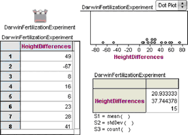
1. Open  Darwin.ftm  from the  Tutorial Starters   folder in the  Sample Documents   folder.  This document contains the data for the experiment described above: 1 attribute, 15 cases.

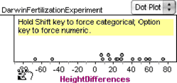
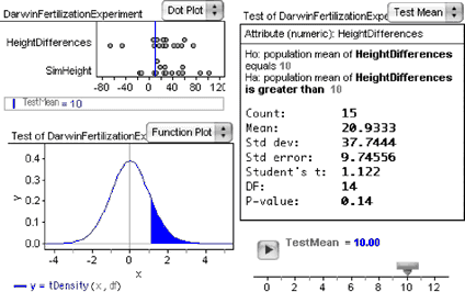
2. Make a case table, a dot plot, and a summary table similar to those shown here.

We see that most of the measurements are greater than 0, meaning that the cross-pollinated plants grew bigger. But two of the measurements are less than 0. Darwin did not feel justified in tossing out these two values and was faced with a very real statistical question.

Formulating a Hypothesis

Darwin’s theory—that cross-pollination produced bigger plants than self-pollination—predicts that, on average, the difference between the two heights should be greater than 0. On the other hand, it might be that his 15 pairs of plants have a mean difference as great as they do (21-eigths of an inch) merely by chance. You can write out these two hypotheses in Fathom in a text object to be stored with your document.

3. From the shelf, drag a text object into the document.

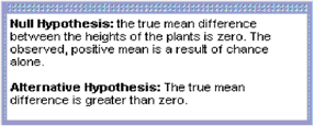
4. Write the null hypothesis and the alternative hypothesis. At right you can  see one way to phrase the hypotheses.

You can choose  Edit | Show Text Palette  to bring up a full suite of tools for formatting text and creating mathematical expressions.

Deciding on a Test Statistic

At the time of Darwin’s experiment, there was no very good theory for dealing with a small sample from a population whose standard deviation is not known. It was not until some years later that William Gosset, a student of Karl Pearson, developed a statistic and its distribution. Gosset published his result under the pseudonym Student, and the statistic became known as Student’s  t . When the null hypothesis is that the mean is 0, the  t -statistic is simply, x ̄/( s /√ n ), where x ̄ is the observed mean,  s  is the sample standard deviation, and  n  is the number of observations.

Let’s compute this statistic for Darwin’s data using one of Fathom’s built-in statistics objects.

5. Drag a test object from the shelf.  An empty test appears.

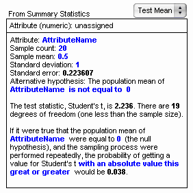
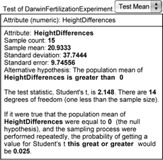
6. From the pop-up menu, choose  Test Mean .  As shown at right, the Test Mean test allows us to type in summary statistics. The blue text is editable. This is very useful when you don’t have raw data.

7. Try editing the blue text. You can, for example, enter the summary statistics for Darwin’s data.

Here are some things to notice.

• Changing something in one part of the test may affect other parts. For example, editing the AttributeName field in the first line also changes it in the hypothesis line and in the last paragraph.

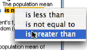
• In the hypothesis line, clicking on the “is not equal to” phrase brings up a pop-up menu from which we can choose one of three options. For Darwin’s experiment, we want the third option because his hypothesis is that the true mean difference is greater than 0 . Notice that making this change alters the phrasing of the last line of the test as well.

• In addition to simple editing of numbers, we can also determine their value with a formula. For example, we might want to tie the sample count to a slider named n so that we could investigate the effect of different sample sizes. To show the formula editor, choose  Edit | Edit Formula  with the text cursor in the number whose value you wish to determine. These computed values display in gray instead of blue. Editing the value itself deletes the formula.

Checking Assumptions

Gosset’s work with the t -statistic relied on an assumption about the population from which measurements would be drawn, namely, that the values in the population are normally distributed. Is this a reasonable assumption for Darwin’s data?

Height measurements of living things, both plants and animals, are usually normally distributed, and so are differences between heights. But we might worry, because the two negative values give a decidedly skewed appearance to the distribution.

Fathom can help us determine qualitatively whether this amount of skew is unusual. We’ll generate measurements randomly from a normal distribution and compare the results with the original data.

8. Make a new attribute in the collection. Call it  simHeight  for simulated height.

9. Select  simHeight  and choose  Edit | Edit Formula . Enter the formula shown below.

This formula tells Fathom to generate random numbers from a normal distribution whose mean and standard deviation are the same as in our original data. We want to compare the distribution of these simulated heights with the distribution of the original data. We can do that directly in the dot plot that already shows  HeightDifferences .

10. Drop  simHeight  on the plus sign to add it to the horizontal axis.  The graph now shows the original data on top and the simulated data on the bottom.

One set of simulated data doesn’t tell the whole story. We need to look at a bunch.

11. Choose  Collection | Rerandomize .

Each time you rerandomize, you get a new set of 15 values from a population with the same mean and standard deviation as the original 15 measurements. Three examples are shown below.

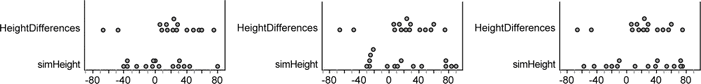
A bit of subjectivity is called for here. Does it appear that the original distribution is very unusual, or does it fit in with the simulated distributions?

Testing the Hypothesis

Once we have decided that the assumption of normality is met, we can go on to determine whether the  t -statistic for Darwin’s data is large enough to allow us to reject the null hypothesis.

In step 7, we typed the summary values into the test as though we didn’t have the raw data. But we are in the fortunate position of having the raw data, so we can ask Fathom to figure out all the statistics using that data.

12. Drag   HeightDifferences  from the case table to the top pane of the test where it says “Attribute (numeric): unassigned.”

13. If the hypothesis line does not already say “is greater than,” then select that choice from the pop-up menu.

The last paragraph of the test describes the results. If the null hypothesis were true and the experiment were performed repeatedly, the probability of getting a value for Student’s  t  this great or greater would be 0.025. This is a pretty low  P -value, so we can safely reject the null hypothesis and, with Darwin, pursue the theory that cross-pollination increases a plant’s height compared with self-pollination.

Looking at the t -Distribution

It is helpful to be able to visualize the P -value as an area under a distribution.

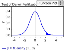
14. With the test selected, choose  Test | Show Test Statistic Distribution .  The curve shows the probability density for the t -statistic with 14 degrees of freedom. The shaded area shows the portion of the area under the curve to the right of the test statistic for Darwin’s data. We’ve set this up as a one-tailed test; we’re only interested in the mean difference being greater than zero. The total area under the curve is 1, so the area of the shaded portion corresponds to the P -value for Darwin’s experiment.

Let’s investigate how the P -value depends on the test mean, which is currently set to 0.

15. Drag a slider from the shelf into the document.

16. Edit the name of the slider from  V1  to  TestMean .

17. Select the 0 in the statement of the hypothesis in the test. Choose  Edit | Edit Formula .

18. In the formula editor, enter the slider name   TestMe an  and click  OK .

Now the value of the null hypothesis mean in the test and the shaded area under the  t -distribution change to reflect the new hypothesis.

19. Drag the slider slowly and observe the changes that take place.

For what value of the slider is half the area under the curve shaded? Explain why it should be this particular value.

The illustration below shows something similar to what you probably  have. Note that the test has been switched to “nonverbose” (choose  Test | Verbose ).

Going Further

• Play around with changing the data and observing the effect on the P -value. How much closer to 0 can the experimental mean be (without changing the standard deviation) and still have a  P -value greater than 0.05? If you make the standard deviation smaller, what happens to the  P -value (and why)?
• Make a Test Mean object that tests the mean of   simHeight   instead of   HeightDifferences . Notice that each time you rerandomize, you get a new  P -value. Think about what it means when the P -value is greater than 0.05. Would you call this a “false positive” or a “false negative”? By repeatedly rerandomizing, estimate the proportion of the time that the P -value is greater than 0.05. What practical significance would that have in planning an experiment?

An official website of the United States government

The .gov means it’s official. Federal government websites often end in .gov or .mil. Before sharing sensitive information, make sure you’re on a federal government site.

The site is secure. The https:// ensures that you are connecting to the official website and that any information you provide is encrypted and transmitted securely.

• Publications
• Account settings

Preview improvements coming to the PMC website in October 2024. Learn More or Try it out now .

• Advanced Search
• Journal List
• Plants (Basel)

Reaching Natural Growth: Light Quality Effects on Plant Performance in Indoor Growth Facilities

Camilo chiang.

1 Department of Environmental Sciences—Botany, University of Basel, Schönbeinstrasse 6, 4056 Basel, Switzerland; [email protected]

2 Department of Research and Development, Heliospectra, Fiskhamnsgatan 2, 414 58 Gothenburg, Sweden; [email protected]

Daniel Bånkestad

Günter hoch, associated data.

To transfer experimental findings in plant research to natural ecosystems it is imperative to reach near to natural-like plant performance. Previous studies propose differences in temperature and light quantity as main sources of deviations between indoor and outdoor plant growth. With increasing implementation of light emitting diodes (LED) in plant growth facilities, light quality is yet another factor that can be optimised to prevent unnatural plant performance. We investigated the effects of different wavelength combinations in phytotrons (i.e., indoor growth chambers) on plant growth and physiology in seven different plant species from different plant functional types (herbs, grasses and trees). The results from these experiments were compared against a previous field trial with the same set of species. While different proportions of blue (B) and red (R) light were applied in the phytotrons, the mean environmental conditions (photoperiod, total radiation, red to far red ratio and day/night temperature and air humidity) from the field trial were used in the phytotrons in order to assess which wavelength combinations result in the most natural-like plant performance. Different plant traits and physiological parameters, including biomass productivity, specific leaf area (SLA), leaf pigmentation, photosynthesis under a standardised light, and the respective growing light and chlorophyll fluorescence, were measured at the end of each treatment. The exposure to different B percentages induced species-specific dose response reactions for most of the analysed parameters. Compared with intermediate B light treatments (25 and/or 35% B light), extreme R or B light enriched treatments (6% and 62% of B respectively) significantly affected the height, biomass, biomass allocation, chlorophyll content, and photosynthesis parameters, differently among species. Principal component analyses (PCA) confirmed that 6% and 62% B light quality combinations induce more extreme plant performance in most cases, indicating that light quality needs to be adjusted to mitigate unnatural plant responses under indoor conditions.

1. Introduction

Temperature and light are principal determinants of plant growth, as plants react to environmental conditions in their development. With improvements in controlled environment facilities, the use of indoor cultivation systems has increased worldwide, both for research and plant production. One of the problems, that especially plant researchers are confronted with, is a clear difference between plants grown under indoor versus outdoor conditions. These differences are limiting the transferability of results from indoor experiments to natural systems. Several experiments have tried to replicate outdoor growth in indoor facilities, but low correlations have been found [ 1 , 2 ]. Poorter et al., [ 3 ] suggested that this difference comes mainly from the different photothermal ratio (PTR), the ratio between the daily light integral and the daily mean temperature, which is generally much lower in growth chambers. The low PTR in indoor experiments mainly derives from the low and constant irradiances used, compared with the higher and variable sunlight conditions found in nature. In general, conditions in indoor facilities lead to higher specific leaf area (SLA), leaf nitrogen content, and relative growth rate. While maximum photosynthesis (A max ), plant height, and shoot dry weight (SDW), are lower compared with outdoor experiments [ 3 ].

Due to the high photosynthetic efficiency of blue (B) and red (R) light, high electrical efficiency of B and R LEDs, as well as the high technical requirements to create sun-like LED spectra [ 4 , 5 ], most existing indoor plant growth facilities with LED lighting systems use mixtures of mainly B and R light. However, different LED lamps use different proportions of B and R LEDs, or B and R in combination with other LED types, such as white and far-red. This results in very different lighting environments among different indoor growth facilities. In addition, the lack of a common protocol for reporting and measuring LED light irradiance further limits the comparability between experiments [ 6 ]. Many studies have investigated plant response to different B to R ratios. These studies revealed that independent of light intensity, a required minimum percentage of B light is necessary to maintain the activities of photosystem II and I [ 7 ]. Hogewoning et al., [ 8 ] suggested that at least 7% B light is necessary to reproduce near-natural plant growth. In addition, it has been observed that long exposures of monochromatic light can have drastic effects, including non-natural morphologies. With parameters such as shoot elongation, specific leaf area (SLA), chlorophyll concentration and photosynthetic performance being affected [ 9 , 10 , 11 , 12 ].

The vast majority of studies related to light quality effects on plants have been conducted under low light levels, varying between 20 to 330 µmol m −2 s −1 [ 13 , 14 , 15 , 16 , 17 , 18 ], with a few exceptions (for example 550 µmol m −2 s −1 [ 19 ]), even though interactions between light quantity and quality have been reported previously [ 9 ]. Finally, it is also important to consider other light quality related parameters, for example, the effect of red to far red ratio (R:FR). The applied light conditions in indoor cultivation typically has a much higher R:FR ratio (or a complete absence of FR) compared with sunlight conditions. This affects plant photosynthesis, morphology, and development (for example [ 8 , 10 , 14 , 15 , 18 , 19 , 20 ]). Once the R:FR ratio is corrected to more natural values, a more natural-like growth may be achieved, despite the large deviations from natural sunlight in other parts of plant biologically active radiation (280–800 nm; for example [ 21 ])

The aim of this study is to provide the first step in a series of experiments with the overall goal of reaching nature-like growth of plants under indoor conditions. Specifically, we investigate the effects of varying proportions of B and R light within walk-in growth chambers (phytotrons) on growth and physiological traits of plants from different functional groups. We also compared our findings to the same species grown in a natural-light field trial, where we expected more “natural-like” growth in our indoor treatments that applied a closer to natural light spectra. The inclusion of seven different species from different functional plant types further enabled us to identify if light quality affects plant performance differently among species and plant types. In contrast to many previous studies, we explicitly applied more natural-like R:FR ratios and light intensities [ 8 , 9 , 10 , 11 , 12 , 13 , 14 ], and the plants were exposed to temperatures and air humidity based on the pre-measured field trial.

2.1. Light Treatments

Four different treatments were obtained through calibrating the phytotrons for the desired spectra as indicated in Table 1 and Figure 1 .

Applied spectra for the field trial and each of the different light treatment where 6%, 25%, 35% and 62% refers to the percentage of blue light as percentage of the photosynthetic photon flux density (PPFD) (In other words, excluding far-red). The integrated area between 400 and 700 nm corresponds to an approximate 575 μmol m −2 s −1 of photosynthetic photon flux density in each case.

Spectral characteristics of sunlight and of the indoor light treatments, based on the measured spectra shown in Figure 1 .

2.2. Plant Growth and Biomass Allocation

There was a significant interaction between the light treatments and the different species on the total plant height at the end of the experiments ( Table 2 ), where the relationship with the field trial was species dependent. Some species, for example, Alnus and Melissa , were significantly smaller independent of the light treatment, while others, for example, Ocimum , were taller than the same species in the field trial.

p -values derived from the full-factorial ANOVA analyses of the different measured plant traits, with light treatment and species as fixed factors, and the replicates of the individual light treatments as random factors. Non-significant p -values (≥0.05) are indicated as “-”.

* Lettuce was removed from these analyses. ** Interactions or factors were removed from the analysis due non-significance.

Comparing only among the phytotron treatments, all species had shorter individuals at higher percentages of blue (B) light (62%), which was most pronounced in Alnus and Melissa (58 and 52% lower height respectively, compared with the 6% B treatment; Figure 2 A). Other species like Ocimum and Triticum were less affected by changes in B light, but follow the same trend (20 and 15% lower height respectively, compared with the 6% B treatment; Figure 2 A). In several of the tested species, there was a significant difference in plant height between the two intermediate B treatments (25 and 35% B). Averaged across species, 6% B light produced 22% taller plants that were statistically significantly different from the two intermediate treatments. While in the other extreme, 62% B light yielded a statistically significant shortening of plants by approximately 20% compared with the average across treatments ( Figure 2 A). A dose response was obtained for specific leaf area in several species (SLA, Figure 2 B). Unlike the height results, and due to the species-specific reactions to the light treatments, the average response across species did not significantly differ, neither within the light treatments, nor between the light treatments and the outdoor control. However, Lactuca and Alnus, for example, had significant higher SLA at 6% B compared with other light treatments, while other species, for example, Raphanus and Triticum, had higher values at 25 or 35% B light compared with 6 or 62% B light.

Fold change on: plant height ( A ) and SLA ( B ), relative to the average field trial (dotted line). Coloured dots are the average of each species in both experiment runs ( n = 18), the black dots are the average values across all 7 species ( n = 126). Error bars indicate the standard errors. The grey area corresponds to the standard error of the field trial. Different letters indicate statistical difference between groups with experiment replicate and species as a random effect.

There were significant interactions between the light treatments and species for the dry biomass of leaves, shoots, roots and the total dry biomass ( Table 2 ). Similar to plant height and SLA, the relationship between plant biomass and light, under the different light treatments, with the field control was species dependent, yet averaged across all species. Leaf biomass did not significantly differ from the outdoor control in any of the light treatments.

If only the phytotron treatments are compared, there was a lower leaf biomass under 62% B light compared with 6% B light in all investigated species. This was especially the case for the two tree species tested, where Alnus and Ulmus were most sensitive to high percentages of B light ( Figure 3 A). On average, plants exposed to 6% B had 35% higher leaf biomass than plants exposed to 62% B ( Figure 3 A). Similar results were obtained for shoot biomass where, across all species, plants grown at 62% B had a significantly lower shoot biomass compared with all the other light treatments, and yet similar values as in the field trial (except for Ulmus and Ocimum , Figure 3 B). In contrast to the aboveground biomass, the effects of light quality on root biomass were different among all species ( Figure 3 C). In comparison to the field trial, four species ( Ulmus , Lactuca , Ocimum , Triticum ) had significantly higher root biomass in the phytotron treatments, while in three species ( Raphanus , Alnus , Melissa ) it was similar compared to the field trial ( Figure 3 C).

Fold change on: leaves ( A ), shoot ( B ), roots ( C ) and root to shoot ratio ( D ), as dry weight relative to the average value of the field trial (dotted line). Coloured dots are the average of each species in both experiments runs ( n = 18), the black dots are the average values across all 7 species ( n = 126). Error bars indicate the standard errors. The grey area corresponds to the standard error of the field trial. Different letters indicate statistical difference between groups with experiment replicate and species as a random effect.

Across all species, there was no strong effect of light quality on root biomass, but a trend to higher root biomass at 6% B ( Figure 3 C). Total biomass production followed the same trend as found for the individual plant organs, with a significant interaction between light treatment and species ( Table 2 ); higher values under indoor conditions independent of the light treatment, compared to the field trial and increasing biomass with increasing percentage of blue light (data not shown).

With respect to the effect of light quality on the allocation of biomass, there was a significant interaction between light treatment and species for the root to shoot (r:s) mass ratio ( Table 2 ). Almost all species had significantly higher r:s values in the phytotrons compared to the field trial independent of the light treatment, with Triticum showing a four to eight times higher investment in roots compared with the field control ( Figure 3 D). In some species (e.g., Alnus and Ocimum ), 6% and 62% B light induced higher r:s ratios than 25 and 35% B light, while other species (e.g., Melissa and Ulmus ) were almost indifferent with respect to light quality ( Figure 3 D).

2.3. Leaf Pigmentation

There were significant interactions between the different treatments and species in the pigment concentrations of the leaves ( Table 2 ). Furthermore, the difference between the field trial and the different light treatments was species dependent, but all investigated species exhibited higher Chl a concentration in leaves at 62% B light compared to the other light treatments (strongest effect in Lactuca ) and several species exhibited the lowest Chl a concentrations at 6% B light ( Figure 4 A).

Fold change on Chlorophyll a ( A ), Chlorophyll a:b ratio ( B ), carotenoids content ( C ) and Fv/Fm values ( D ) relative to the average value of the field trial (dotted line). Coloured dots are the average of each species in both experiments runs ( n = 18), the black dots are the average values across all 7 species ( n = 126). Error bars indicate the standard errors. The grey area corresponds to the standard error of the field trial. Different letters indicate statistically difference between groups with experiment replicate and species as a random effect.

On average across all species, 6% B was the only treatment significantly different from the field trial, with 24% lower concentration of Chl a. The effect on Chl b was similar to that of Chl a, with a smaller effect of the light quality on the total amount of Chl b (data not shown). As a result, the average a:b ratio across all species was not significantly different among the light treatments, but significantly higher than in the field trial ( Table 2 , Figure 4 B). The concentrations of carotenoids in leaves, showed overall very similar reactions to light quality as chlorophyll, with increasing concentrations at higher proportions of blue, and an interaction between the light treatment and species ( Figure 4 C, Table 2 ). Like chlorophyll and carotenoids, the Fv/Fm values, showed significant interaction between the species and the light treatments ( Table 2 ). Almost all species in the phytotron treatments with 25, 35 and 62% B had Fv/Fm values close to the field trial ( Figure 4 D), except Ocimum , which revealed higher Fv/Fm values indoors than in the field. Averaged across all species, Fv/Fm was significantly lower than in the field at 6% B ( Figure 4 D). Performance index (Pi) absolute values followed the same trend as Fv/Fm (data not shown, Supplementary Table S1 ).

2.4. Photosynthesis and Leaf Respiration

In contrast to the other plant traits tested, all species reacted uniformly to the light treatments in all measured photosynthesis and leaf gas exchange parameters, with no significant interaction between treatment and species effect found ( Table 2 ). When measured with the standardised light of the gas exchange chamber, the average maximum photosynthesis (A max ) across all species was significantly higher in plants raised at 62% B compared with the field trial ( Figure 5 A). Meanwhile, when the same parameter was measured under the in situ light, higher values were reached at either 25% or 35% B light compared with the field trial ( Figure 5 B). The quantum yield of the CO 2 fixation (α) had similar trends to A max , where on average no light treatment was significantly higher than the field trial when the standardised light was used. The 62% B light was the only treatment to induce higher α values than the other light treatments ( Figure 5 C). When α was measured using the in situ light, higher values were reached at either 6%, 25% or 35% B compared to the field trial ( Figure 5 D).

Fold change on maximum photosynthesis ( A max , A , B ), quantum yield of the CO 2 fixation curve (α, C , D ) and dark respiration (DR, E , F ) relative to the average value of the field trial (dotted line). Values were measured with either a standard light with 70% B light and 30% R light (‘standardised light’) or the actual ‘in situ’ light (see methods for details). Coloured dots are the average of each species in both experiments runs ( n = 18), the black dots are the average values across all 7 species ( n = 126). Error bars indicate the standard errors. The grey area corresponds to the standard error of the field trial. Different letters indicate statistical difference between groups with experiment replicate and species as a random effect.

The photosynthetic light compensation point (CP) and the dark respiration of leaves (DR) were significantly different among species ( Table 2 ). Averaged across all species, there were no significant effects of the treatments on CP when the standardised light was used. However, with in situ light significantly lower values were reached under 6 and 25% B conditions, compared with 35 and 62% B and the field trial (data not shown). DR was on average significantly lower in plants exposed to 62% B light compared with other light treatments and the field trial when the standardised light was used ( Figure 5 E). This was not the case for the in situ light, where although several species had higher DR values than the field trial, no significant difference was found between the treatments for the average across species ( Figure 5 F).

2.5. Principal Component Analysis (PCA)

Principal component analysis (PCA) for each species revealed a clustering of each treatment with varying degrees of overlap ( Figure 6 ); from easily differentiable groups between light treatments in some species, for example, Alnus , Lactuca and Triticum , to a more continuous gradient among treatments.

Principal component analysis (PCA) of the measured traits of each species: ( A ) Alnus , ( B ) Ulmus , ( C ) Ocimum , ( D ) Lactuca , ( E ) Melissa , ( F ) Raphanus and ( G ) Triticum , grown under 6% B, 25% B, 35% B and 62% B light. Each lighter point ( n = 18) corresponds to a plant and solid ones to the average weighted centroids of each light treatment, where the name of each species is mentioned in the respective upper right corner. Ellipses correspond to the standard error of the weighted centroids with a confidence interval of 95%.

Melissa , Raphanus , Alnus , Ocimum , Lactuca , and Triticum showed a large variability between treatments from outdoor (field trial) to indoor conditions, while the different light treatments tended to cluster. This was not the case for Melissa , Raphanus , and Ulmus , where the field trial was not clearly separated from the phytotron treatments ( Figure 6 ). The two intermediate treatments (25% and 35% B) yielded responses closer to the average (i.e., the centre of the figure) in most species. The loadings for score calculations were also plotted to determine the importance of each factor. No single parameter was specifically responsible for the variation across treatments and between species, except for CP in Ocimum growing in the field trial ( Figure S1 ). Independent of the species the first two components explained between 31% and 43% of the total variability.

3. Discussion

Previous studies investigating the effect of the spectral light quality on plant performance were mainly focused on single species, and they generally did not directly compare findings with natural conditions. In the present study, we deliberately investigated a suite of species from different functional plant types to determine if, and how, they react to the different treatments. Through application of the same mean climatic conditions indoors, as in the initial field trial, we could better assess which LED light conditions are generating the most natural-like plant performance. Our results showed clear differences within and between the light treatments when compared to the field trial on most measured plant traits. The effect sizes were highly species-specific, while effect directions were similar among species, with the clear exception of SLA and root biomass production. As expected, light treatments with very extreme blue: red (B:R) ratios (6 and 62% B) induced more extreme (‘unnatural’) values in most plant traits than treatments with a more balanced B:R ratio (25 and 35% B).

3.1. Light Quality Effects on Morphology

Studies that compared indoor with outdoor plant growth were previously often biased by a higher plant density in the indoor condition [ 3 ]. In our study, we deliberately kept the exact same plant densities between the field and the phytotron trials to avoid any stand density bias on plant morphology. The effects of B light percentages on plant morphology have been previously reported in several studies [ 8 , 11 , 12 , 21 , 22 , 23 , 24 , 25 ]. In general, B light is sensed by the cryptochrome system, where under high irradiances or high levels of B light, plants exhibit shorter and stunted growth (For example [ 8 , 14 , 26 ]). It is also known that a total lack of B or R light negatively affects plant performance, including growth rate, height, photosynthesis and several other parameters. For example, Hernandez et al. [ 10 ] found that tomato plants grew shorter under either B or R light mixtures compared with only B or R light.

Previous studies have shown that under high levels of B light, there is an increase in the palisade cell area, which can lead to an increase in leaf thickness (For example [ 8 , 10 , 12 ]). However, this B light-induced increase in leaf thickness does not necessarily have to translate into a lower SLA [ 27 ]. Dougher and Budgee [ 22 ] identified that the direction of the effect of B light on SLA is very species dependent. Independent of the applied light quality, Poorter et al. [ 3 ] found that on average, indoor experiments tend to produce plants with higher SLA compared to field grown plants, mainly due to higher temperatures and lower light quantity in indoor facilities. In our study, which applied the average temperature and light quantity as in the field trial, the SLA of most species was similar between plants growing in the phytotrons and in the field.

Under the different treatments stem, leaf, root, and total dry biomass largely followed the trend in plant height. The lower biomass at high B% can thus be explained by a stronger inhibition of stem elongation by B light due to an increased cryptochrome activity [ 14 ], exposing the plants to lower irradiance due to larger distances to the light source compared with plants treated under a lower percentage of B light. In addition, the stunted growth of plants at high B% leads to an increased self-shading of leaves and decrease in light interception, which has been proposed to result in negative consequences for the whole plant productivity [ 21 ]. Although the individual species reacted differently between phytotrons and the field trial, on average, a significantly higher plant biomass within our phytotron treatments compared with the field was found (except for the 62% B treatment). In contrast, Poorter et al. [ 3 ] reported lower biomass under indoor conditions compared with field grown plants depending on species and functional group. Again, this apparent contradiction could be explained by the fact that in contrast to other indoor experiments, we deliberately applied the same average temperatures and light strength in the phytotrons as were measured in the field trial. Poorter et al. [ 3 ] demonstrated that indoor experiments often use low levels of light, which might reduce plant biomass in comparison with outdoor-grown plants.

While the effect of light quality on the aboveground organs was quite similar among species in the current study, the direction of the effect on roots was clearly species dependent. With species such as Alnus and Ocimum exhibiting higher root growth at very low and high B%, and species such as Raphanus and Ulmus showing increased root production at intermediate B percentages (25 and 35% B). To date, scarce information is available on the effects of light quality on belowground plant productivity. A previous study by Yorio et al. [ 28 ] reported that under 10% B mixed with 90% R light there was a higher root production in Lactuca, Raphanus, and Spinacia, compared with plants grown under pure R light. Nhut et al. [ 29 ] found that mixtures of B and R light stimulate the production of roots compared with pure R light in strawberry plantlets. Independent of light quality, we found a significantly enhanced root production in the phytotron treatments compared to the field grown plants, except for the 62% B treatment. As indicated by Poorter et al. [ 3 ], indoor climatization might induce root zone conditions that differ markedly from field conditions, leading to altered root production and consequently profoundly changed plant growth. As all plants in our experiment were regularly watered in both field and phytotron treatments, we can exclude that the observed higher root productivity in the phytotrons results from different water availability between indoor and field trials. However, pot soil temperature was not monitored, and it is possible that it differed significantly between indoor and field conditions, partly due to the lack of infrared radiation from the LED lamps.

3.2. Light Quality Effect on Leaf Pigmentation

The concentration of chlorophyll and carotenoids changed strongly with light quality in our study. Under natural sunlight, cryptochrome activity is reduced at high radiation, thereby signalling strong light conditions in the plant. The same effect can be achieved under experimental conditions by exposing plants to high percentages of B light [ 30 ]. The high proportion of B light in our 62% B treatment thus triggered the enhanced production of photosynthetic pigments despite the fact that the other treatments with lower B% had the same PPFD. In fact, the low concentrations of Chl a and b in plants that have been treated with low levels of B light or monochromatic R light in previous studies, have even led to photo-oxidative stress in plants due to an increase of O 2 - and H 2 O 2 radicals that induce cellular damage [ 8 , 19 ]. Barnes and Bugbee [ 30 ] proposed that a minimum of 20−30 μmol m −2 s −1 of B light is necessary to reach natural-like growth and morphologies, even if such a minimum requirement for B light appears to be highly species-specific [ 31 ]. It is likely that due to all of our light treatments including at least 6% of B light, we did not observe light quality related stress effects in our experiment. However, we identify that even with over 30 μmol m −2 s −1 of B light (at 6% B), higher percentages of B can increase the photosynthetic maximum capacity in several species, indicating that it is not just the quantity of B light, but also its relationship with other wavebands in the spectrum. Interestingly, most species showed higher Chl a:b ratios in the phytotrons compared to the field trial. This effect has been observed previously in indoor-grown plants [ 32 ], where it is attributed to the lack of fluctuating light conditions in indoor facilities.

Like chlorophyll, the production of carotenoids was also significantly increased with 62% of B light compared to 6% B (and 35% B), yet only the 25% B and the 62% B treatments induced higher carotenoid concentrations than in the field trial. Hogewoning et al. [ 8 ] reported an increase of carotenoids in cucumber plants when B was increased to 50% in the light spectra. An increase of carotenoids has been shown to work as an accumulative protection mechanism correlating with high light intensities or high B ratios. For example, the authors of [ 12 ] found that Fv/Fm of rapeseed leaves was reduced under monochromatic B or R light treatments, compared with mixtures of B and R. They attributed this to a higher PS II damage and linked the higher concentrations of carotenoids to a protection mechanism against oxygen radical formation. This is in line with our Fv/Fm results, where lower percentages of B in the applied spectra induce small but significant differences of the Fv/Fm values in almost all investigated species.

3.3. Light Quality Effects on Photosynthesis

When A max was measured under the same standardised light conditions (30% B and 70% R) in the current study, plants under 63% B showed, on average, significantly higher A max compared to plants under 25% B and the field trial. This could be partially explained by the increased chlorophyll concentrations in 63% B treated plants (see above). Previously, higher A max have been linked to higher levels of stomatal conductance and nitrogen concentration, where the latter is correlated to Rubisco, cytochrome, proteins and chlorophyll content [ 33 ]. A higher A max has also been suggested to partially derive from an instantaneous stimulation of photosynthesis (i.e., during the exposure to the light within the gas-exchange chamber) due to the lack of adaptation to the standardised light condition [ 8 ]. In our case, using 70% R in plants adapted to 62% B may promote a higher A max , meanwhile this may not be the case in plants adapted to lower percentages of B light, and therefore higher percentages of R light. Kim et al. [ 15 ] have shown that in Pisum sativum about four days were necessary to reach full photosynthetic acclimation after a transition from a PSI to a PSII stimulating light environment and vice versa. Similarly, Hogewoning et al. [ 34 ] showed in duckweed, that six days were needed to fully acclimate to different light conditions, using the Chl a:b ratio as the control parameter.

In contrast to the measurements of standardised light, when measured under the respective in situ light conditions, A max was significantly lower at very low (6%) or very high (62%) B light conditions, despite the higher concentration of chlorophyll at 62% B or small differences in SLA ( Figure 2 B). In a similar but more extreme experiment, several long-term studies reported lower net photosynthesis or A max in plants raised under monochromatic B or R light [ 8 , 11 , 12 ]. Hogewoning et al. [ 8 ], also reported dysfunctional photosynthesis in cucumber plants, grown under pure R light and a dose response curve in A max when the B% was increased up to 50% B, with no further increase of A max beyond 50% B. The increase of A max with B percentages was associated with a reduction of the SLA, an increase of N and chlorophyll per leaf area, and higher stomatal conductance under mixtures of B and R light compared with only B or R [ 8 ]. Matsuda et al. [ 35 ] reported an increase of A max in spinach plants exposed to a 1:1 B: R radiation compared with just B light, associated with increased leaf N concentration. Shengxin et al. [ 12 ] showed that dark adapted Fv/Fm values were higher (as an indicator for less photo-stress) under mixtures of B and R light compared with monochromatic B or R light.

The effects of treatments on photosynthesis were also visible in the quantum yield of the CO 2 fixation curve (α) of the investigated species. Similar to A max , a more natural level of B light may explain a higher efficiency when an ‘in situ’ light was used for our gas-exchange measurements, with significantly higher values indoor than in the field trial. Similar results have been reported at 15–30% B compared with 50% B [ 8 ]. This effect may indicate the evolutionary adaption of species to the natural sunlight spectrum, with higher quantum yield under a more natural B:R ratio (circa 33% of B in the sunlight spectrum [ 36 ]). Other conditions with extreme levels of B or R light may require the adaptation to each light condition, where CO 2 fixation may have a wavelength dependence related to absorption properties of the different pigments involved. Terashima et al. [ 37 ], described three major causes for the wavelength dependency of the quantum yield: absorption by photosynthetic carotenoids, absorption by non-photosynthetic pigments and an imbalanced excitation of the two photosystems, where an imbalance in excitation will result in quantum yield losses [ 27 , 38 ]. It has been shown that a correct light stimulus, with light qualities matching the species-specific ratio of PSII and PSI, is key to high quantum efficiency of photosynthesis [ 39 ]. The light compensation point of photosynthesis (CP) was generally not affected by light quality. Similar results have been observed in previous cases [ 9 , 12 ].

In the current study, the average dark respiration (DR) using the standardised light, independent of the species, was relatively lower at 62% B compared with the other light treatments or the field trial. Atkin et al. [ 40 ] described in tobacco that observed changes in DR were dependent on the previously applied irradiance (tested between 0 to 300 μmol photons m −2 s −1 ). An instantaneous stimulation of the photosystems in low light adapted plants due the stimulus of an intensity radiation burst was hypothesised. Although the total photon flux was the same between treatments in our study, similar short time effects on DR might have occurred when plants were exposed to a high intensities and light spectrum that they were not adapted to.

3.4. Principal Component Analysis

The PCA analyses performed in this study confirmed that the effects of light quality on plant performance are highly species dependent, and adjustments of the light spectra may help to promote more natural like growth, where more natural growth like plants tend to group closer to the field trial in the PCA. Applying a light spectrum with similar B and R light proportions to sunlight is proposed to avoid physiological plant responses to a lack or excess of B light (which might also differ among species). Although 7% B has been recommended to avoid dysfunctional photosynthesis [ 8 ], this study indicates that levels of 25 to 35% B light in the spectrum are needed in indoor conditions to avoid undesired (i.e., unnatural) effects of the light spectrum on plant growth. This was demonstrated with higher distances of the 6%B light treated plants from the field trial plants in the PCA. No specific trait was identified across the different species to have a higher importance than others ( Figure S1 ), where the ranking of importance of each measured parameter was species dependent. Independent of this, the PCA clearly indicated that other environmental variables should be controlled (e.g., air flux, soil temperature) or more precisely mimicked in indoor growth facilities if natural-like growth is required. A similar approach has been previously used [ 41 ] to understand the difference between indoor and outdoor experiments, with a focus on Arabidopsis ’s metabolism where a clearer clustering of the indoor and outdoor conditions was obtained. Similar values of the first and second component to the ones presented here (first and second component explaining 28 and 15% of the variance, respectively compared with 24 and 15% average across species in our study).

4. Materials and Methods

4.1. plant material and pre-growing conditions.

In this study, we investigated young plants of 7 species from different functional plant types to include the species as the source of variation: trees represented by black alder ( Alnus glutinosa (L.) Gearth, provenance HG4, Zurich, Switzerland), Scotch elm ( Ulmus glabra Huds., provenance Merenschwand, Aargau, Switzerland), herbs represented by basil ( Ocimum basilicum ‘Adriana’), lettuce ( Lactuca sativa ), melissa ( Melissa officinalis ), radish ( Raphanus raphanistrum subsp. sativus (L.) Domin), and grasses represented by winter wheat ( Triticum aestivum ). For the experiments, all plants were raised from seeds. The seeds of both tree species were purchased from the Swiss federal institute for forest, snow and landscape research, WSL, Birmensdorf, Switzerland. All herb seeds were provided from Wyss Samen und Pflanzen AG, Zuchwil, Switzerland, and Triticum seeds were supplied form Sativa AG, Rheinau, Switzerland. Hereinafter, the species will be referred to by their scientific genus name for clearness. Due to the different germination speeds the timing of sowing was different for the species as follows: seeds of Alnus and Ulmus were sown in 20 × 40 × 2 cm trays with commercial substrate (pH 5.8, 250 mg L −1 N, 180 P 2 O 5 mg L −1 , K 2 O 480 mg L −1 , Ökohum, Herrenhof, Switzerland) 43 days before the start of the experiments and were left to germinate under 190 μmols m −2 s −1 of photosynthetic photon flux density (PPFD: 400–700 nm) with 25% Blue (B: 400–500 nm), 32% Green (G: 500–600 nm) and 41% Red (R: 600–700 nm) light and an R to far red (FR: 700–800 nm) ratio (R:FR. 655–665 nm and 725–735 nm; according to [ 42 ]) of 5.1 for 23 days, using LED lighting with a day length of 16 h. Twenty days before the start of the experiment, the light was increased to 240 μmols m −2 s −1 PPFD, with a R: FR of 5.1, to acclimate the plants to higher intensity levels. Thirteen days before the start of the experiment Melissa seeds were sown in the same type of trays and keeping the last-mentioned environmental conditions. Six days before the start of the experiments the remaining species were sown in the same type of trays and under the same environmental conditions, with the exception of Triticum, which was sown immediately in round 2 L pots with a density of 15 seeds per pot (13.5 cm diameter, Poppelmann, Lohne, Germany). All light measurements were done using a using a spectrometer (STS, OceanOptics, Florida, United States). During the germination and the pre-treatment period, the different seedlings were raised at 25 °C/50% relative humidity (RH) during daytime and 15 °C/83% RH during night, with 10 h per day and one-hour light/temperature/humidity ramping pre and post day.

At the start of the experiment, all species, excluding Triticum , were transplanted to the same type of 2 L pot previously used for Triticum, with a single individual in each pot. Moreover, Triticum was thinned to 10 plants per pot. The pots were filled with the same substrate as used in the germination trays, and 4 g of Osmocote slow release fertiliser (Osmocote exact standard 3–4, Scotts, Marysville, OH, USA), containing 16% total N, 9% P2O5, 12% K2O and 2.5% MgO, was added to each plot. All plants were watered daily in the morning throughout the experiment.

The pre-growing procedure was repeated 3 times for this study: First, for the field-trial that was used as reference for the phytotron experiments, and then twice for the different light treatments of the phytotron experiment. (See control and light quality treatments below). No significant difference in initial height or biomass was found at the start of the experiments within species for the different replications (data not shown).

4.2. Control and Light Quality Treatments

To establish a control treatment as a reference point for natural growth, all seven target species were grown in a field trial for 35 days (4 August 2017–7 September 2017) at the botanical garden of the University of Basel, Switzerland. Throughout the field trial, the in situ climate and the natural sunlight spectrum was recorded ( Figure S2 and below). Following the field trial, we exposed plants from the seven different species to four mixtures of B and R light, which can be expressed as a B/R ratio, or as percentage of B light in four walk-in Phytotrons (1.5 m × 2.5 m) with full control of temperature, air humidity and light quality and quantity (prototypes, Enersign GmbH, Basel, Switzerland). To unify nomenclature with previous studies, the four different light treatments will be referred to by their respective B light proportion ( Table 1 ). The light treatments were chosen based on previous literature (e.g., Hogewoning et al. [ 8 ]), measurements of natural light completed in situ [ 36 ], and technical capacities of the phytotrons at the average light intensity of the outdoor treatment. For each treatment, the replication per species was 9 pots (with either one or more individuals per pot depending on species; see above). In all light treatments, the average PPFD from the field trial (575 μmol m −2 s −1 ) was provided at the average height of the different species using 18 LED panels for each chamber consisting of a mixture of B (400–500 nm) , White (2500 K), R (600–700 nm) and FR (700–800 nm) LEDs per panel (prototypes, DHL-Licht, Hanover, Germany). The LED lighting system of each chamber was mounted on movable ceilings, the height of which can be adjusted through the environmental control software of the chambers. To preserve similar light levels at average plant height, the height of the lamps was adjusted twice during the experiment. Based on the field trial conditions, the day length was set to 13 h and 5 min, giving a constant daily light integral (DLI) of 27.1 mol m −2 day −1 in all light treatments. Similar to the light conditions, temperature and humidity during day and night were set to average field trial conditions: 22 °C/66% RH and 18 °C/79% RH, for day and night, respectively, with a period of one-hour ramping before and after daytime. A uniform temperature and humidity distribution within each chamber was ensured by a constant vertical air stream from below. To avoid border and space effects, all plants were randomly distributed within each phytotron on two tables. The tables were rotated by 90° every day. Each light treatment was replicated twice (two separate runs of all four light combinations), where the distribution of the chambers was random between the two runs.

At the end of the 35-day experimental period, a suite of measurements was conducted in the field trial and the phytotron experiments. A description of the measured parameters is given in the following paragraphs. Due to limitations imposed by the lamp characteristics at high intensities, a higher R:FR ratio compared with outdoor (1.8 vs. 1.1) was applied in order to reach the targeted light intensities. No UV light was applied in the phytotrons.

4.3. Climatic Growth Conditions

In order to apply the most natural conditions within the phytotrons, the climate from the field trial at the botanical garden of the University of Basel, Switzerland, was recorded throughout the 35-day growth period ( Figure S2 ). Relative humidity, temperature, and PPFD were measured every 5 min with a weather station (Vantage pro2, Davis, Haywards, CA, USA). In addition, sunlight spectra in the waveband 350–800 nm were recorded every minute using a spectrometer (STS) that was equipped with an optical fiber and a cosine corrector (180º field-of-view; CC-3-UV-S, OceanOptics) placed by the weather station’s PAR sensor facing upwards. The spectrometer was connected to a Raspberry Pi 2 computer for automatic sampling, integration time adjustments and data storage. A posteriori, the spectra were used to calculate photon flux densities within specific wavebands: PAR, B, G, R and FR. The PAR light measurements were verified by comparing the data from the weather station with the data from the spectrometer readings. The data from the field trial were used to calculate average diurnal and nocturnal temperature, air humidity and PAR conditions for the phytotron treatments.

4.4. Morphological Parameters

By the end of the 35-day growth period, plant height was measured as total height from the substrate to the apical tip. In the case of long inflorescences ( Raphanus ) or plants without a clear stem ( Triticum ), extended leaf length was recorded as height, and in the case of Lactuca , no height was recorded. Two full-grown leaves from the top three mature leaves were collected from each plant to measure leaf area (LI-3100, Licor, Lincoln, NE, USA) and calculate the specific leaf area (SLA) in cm 2 g −1 on a dry leaf weight basis. Dry weight (DW) was measured separately for leaves, stems and roots after 10 days drying at 80ºC in a drying oven (UF 260, Memmert, Schwabach, Germany). Due to the lack of a clear stem, only total aboveground and root biomass were measured for Lactuca , Melissa and Triticum . All reported organ weights and the below to above ground biomass ratio (root:shoot-ratio) refer to plant dry mass.

4.5. Chlorophyll Fluorescence and Chlorophyll Content

One night before the end of the experiment, fast chlorophyll fluorescence induction was measured on one of the top three leaves in four randomly chosen plants of each species and treatment by using a continuous excitation fluorometer with an intensity of 3500 μmol m −2 s −1 centred at 627 nm (Pocket PEA, Hansatech instruments Ltd., Norfolk, UK). The plants were dark adapted for at least 20 min before recording photosynthetic maximum quantum yield (Fv/Fm) and the absolute performance index (PI) of the leaves, which has been correlated previously to stress (for calculations and details, see [ 43 ]).

During harvest, two discs of 1.13 cm 2 area from the top four leaves were punched and stored in a 1.5 mL Eppendorf tube together with four to six glass beads of 0.1 mm diameter for later chlorophyll analysis. The tubes were quickly frozen in liquid nitrogen and then kept at −80 °C until analysis. During the day of chlorophyll measurement, the tubes were agitated two times for 10 s to triturate the tissue using a mixing device (Silamat S6, Ivoclar Vivadent, Schaan, Liechtenstein). After adding 0.7 mL of acetone to each tube, they were agitated again for 10 s and then centrifuged at 13,000 rpm at 4ºC for 2 min. A total of 0.25 mL of the supernatant was dissolved in 0.75 mL of acetone, and the sample absorption spectra were measured using a spectrometer (Ultrospec 2100 pro, Biochrom, Holliston, MA, USA). Chlorophyll a and b concentrations, chlorophyll a to b ratio (Chl a, Chl b and a:b ratio, respectively) and total carotenoid concentrations as mg g −1 , were calculated from the spectra using the values at 470, 646 and 663 nm as described in [ 44 ].

4.6. Leaf Gas Exchange

Six days before the end of the experiment, a light response curve of net CO 2 leaf-exchange was measured in one of the top three leaves in three randomly chosen plants per species and treatment using a LI-6800 photosynthesis system (LI-COR, Lincoln, NE, USA). The light response curves were measured under two different light spectra: (i) a standardised artificial light spectrum, composed of 70% R and 30% B (in the following referred to as ‘standardised light’) provided by the chamber head light source to study photosynthesis of the different species under a uniform light spectrum, and, (ii) the respective growing light spectrum (in the following referred to as ‘in situ spectrum’) provided by using a transparent, clear-top chamber head (Clear-top leaf chamber 6800-12A, LI-COR) to study photosynthesis of the different species under their respective growing spectra and avoid any bias on photosynthesis from a non-adapted spectrum. Twelve different light intensities: 2000, 1500, 1000, 800, 600, 400, 200, 100, 50, 25, 10 and 0 μmol m −2 s −1 of PPFD were used for light response curves with the ‘standardised light’ spectrum. Due to lower maximum irradiance in the phytotrons limited by the light quality being applied (see above), the light response curves for the ‘in situ’ growing light were measured only up to a maximum radiation of 700 μmol m −2 s −1 of PPFD (700, 480, 380, 200, 100, 60, 30, 20, 17, 15 and 0 μmol m −2 s −1 of PPFD). All leaf CO 2 -exchange measurements were conducted at 400 ppm CO 2 , 60% relative air humidity and 20 °C leaf temperature, with 60 to 120 s as the threshold for stability after each light change intensity. Stability of readings was assumed when the difference of the slopes between IRGA’s were smaller than 0.5 μmol mol −1 sec −1 and 1 for CO 2 and H 2 O, respectively.

For each light curve, 12 different light models were fitted accordingly [ 45 ], including a model for photo-inhibition [ 46 ]. For each species and treatment, the model with the best fit (lowest sum of squares) was selected (details in [ 45 ]). The selected model was then used to calculate the following four values from the light response curve: maximum photosynthesis within the range of measured light (A max ), quantum yield of the CO 2 fixation (α) as the slope of the linear curve between 0 and 100 μmol m −2 s −1 of PPFD, dark respiration (DR) and the light compensation point (CP) of photosynthesis.

4.7. Statistical Analysis

To evaluate the effect of the light treatments, a two-way analysis of variance (ANOVA) was performed for all measured parameters, considering the species and different treatments as fixed factors and the two replicates of each treatment as a random factor. The significance of the random factor was evaluated using a restricted likelihood ratio test. The data were checked for normal distribution, independence and homogeneity of the variance.

To enable the direct visible and statistical comparison of the treatment effects across species, each measured trait was normalised relative to its mean value on the field trial for each species (the original trait average values per species and treatments are available in Table S1 ). The normalised values were used to perform a one-way ANOVA, considering the treatments as fix factor and species as random factors ( Table S2 ). A Tukey pairwise multiple comparison test was used as post hoc analysis to identify significant differences ( p < 0.05) among treatments. In several cases when all indoor light treatments differed from the field trial, an additional one-way ANOVA was performed without the field trial to highlight the individual response differences to the different light treatments (Data non shown).

Finally, to identify the specific traits that have the maximum variation between treatments and to quantify which treatment gave the overall most similar response compared to the outdoor trial, a principal component analysis (PCA) was performed separately for each species, using the different measured traits as input values. To perform a PCA analysis, the same number of observations is required for each variable but due to fewer photosynthesis measurements, chlorophyll measurements and fluorescence measurements than the number of plants used for biomass measurements, in each species and treatment, the missing values of chlorophyll content and light parameters were imputed using normal distribution with the same average and standard deviation of the available data. All analyses were performed using R [ 47 ] and the package plyr for data processing and lm4, car, RLRsim, emmeans for data analysis and multicomp and vegan for statistically significant representations.

5. Conclusions

The applied light spectra in this study significantly influenced plant morphology, pigment concentration and photosynthesis. Less deviating responses compared to the field trial were reached with either 25% or 35% of B light in almost all species. Hence, if natural like plant growth is desired in indoor plant cultivation, the application of a balanced light spectrum is generally recommended. Despite this, spectral quality of the light source is only one of many factors that can potentially bias plant performance. In this study, we thus aimed to apply similar climatic conditions within the growth chambers as were measured in the field trial to compare outdoor with indoor growth. Nevertheless, we still found significant differences between phytotron and field grown plants in most of the investigated plant traits. This highlights the difficulties to exactly reproduce natural plant performance in indoor growth facilities, as well as the necessity to include the simulation of additional environmental factors (e.g., replication of natural minimum and maximum temperature, humidity and irradiance changes, wind speed and direction) in indoor experiments with plants.

Acknowledgments

We thank Georges Grun and the gardeners at the botanical garden of the University of Basel for their technical support for the phytotron experiments and climate measurements. We also thank Sarah Newberry for proofreading the manuscript.

Supplementary Materials

The following are available online at https://www.mdpi.com/2223-7747/9/10/1273/s1 , Figure S1: Principal component analysis (PCA) of the measured traits of each specie grown under 6% B, 25% B, 35% B and 62% B light, Figure S2. Environmental conditions of temperature (A), air relative humidity (B) and light intensity as PPFD (C) from the field trial, Table S1: Raw average values by measured trial for each treatment and species; Table S2: p -values for the different measured traits in both experiments using normalised data.

Author Contributions

Conceptualization, C.C., D.B. and G.H.; methodology, C.C., D.B. and G.H.; validation, C.C.; formal analysis, C.C.; investigation, C.C.; resources, D.B. and G.H.; data curation, C.C.; writing—original draft preparation, C.C.; writing—review and editing, D.B. and G.H.; visualization, C.C.; supervision, G.H.; project administration, G.H.; funding acquisition, D.B. and G.H. All authors have read and agreed to the published version of the manuscript.

The presented work was supported by PlantHUB-European Industrial Doctorate funded by the H2020 PROGRAMME Marie Curie Action—People, Initial Training Networks (H2020-MSCA-ITN-2016). The programme is managed by the Zurich-Basel Plant Science Center.

Conflicts of Interest

The authors declare no conflict of interest. The funders had no role in the design of the study; in the collection, analyses, or interpretation of data; in the writing of the manuscript, or in the decision to publish the results.

ORIGINAL RESEARCH article

Testing the growth rate hypothesis in two wetland macrophytes under different water level and sediment type conditions.

• 1 Key Laboratory of Agro-ecological Processes in Subtropical Region, Institute of Subtropical Agriculture, Chinese Academy of Sciences, Changsha, China
• 2 School of Environment and Life Science, Nanning Normal University, Nanning, China
• 3 Dongting Lake Station for Wetland Ecosystem Research, Institute of Subtropical Agriculture, Chinese Academy of Sciences, Changsha, China
• 4 College of Architecture and Urban Planning, Hunan City University, Yiyang, China

The growth rate hypothesis (GRH) states that a negative correlation exists between the growth rate and N:P and C:P ratios, because fast-growing organisms need relatively more phosphorus-rich RNA to support their high rates of protein synthesis. However, it is still uncertain whether the GRH is applicable in freshwater wetlands. Several studies have shown that water level and sediment type are key factors influencing plant growth and plant C:N:P characteristics in freshwater wetlands. Thus, this study aimed to elucidate the influence of these factors on plant growth and test the GRH under varying water levels and sediment conditions. We designed a controlled experiment at three water levels and under three sediment types using the two dominant plants ( Carex brevicuspis and Polygonum hydropiper ) in the East Dongting Lake wetland, and we further investigated the relative growth rate (RGR); concentrations of total carbon (TC), total nitrogen (TN), and total phosphorus (TP); and plant stoichiometry (ratios of C:N, C:P, and N:P) in the aboveground and belowground parts and whole plants in both species. Results demonstrated that the RGR and TC of both species decreased significantly with decreasing sediment nutrient supply and increasing water level. However, TN and TP of both species were markedly higher at high water levels than at low water levels; furthermore, these were significantly higher on clay than on the other two sediment types at each water level. The C:N and C:P ratios of both species decreased with increasing sediment nutrient supply and water level, whereas N:P decreased in both species with increasing sediment nutrient supply. The aboveground part of C. brevicuspis as well as the aboveground part and whole plant of P. hydropiper were negatively correlated with N:P, which is consistent with the GRH. However, the relationship between the belowground RGR and N:P of these species was inconsistent with GRH. Therefore, the water level and sediment type and their interaction significantly influenced plant RGR and C:N:P characteristics. The RGR and plant stoichiometry differed significantly between plant organs, indicating that the GRH needs refinement when applied to wetland macrophytes.

Introduction

The growth rate hypothesis (GRH) proposes that fast-growing organisms have low N:P and C:P ratios due to the relatively high demand for phosphorus-rich RNA to support rapid protein synthesis ( Acharya et al., 2004 ). Various comprehensive reviews confirmed that nutrient-rich plants tend to have low N:P ratios, and supported the validity of GRH in the realm of vascular plants, as N concentration in vascular plants tends to increase less than P concentration ( Wright et al., 2005 ; Kerkhoff and Enquist, 2006 ; Yu et al., 2012 ). However, opposite results were also reported ( Peng et al., 2010 ; Loladze and Elser, 2011 ). For instance, Matzek and Vitousek (2009) found that there was no link between growth rate and leaf N:P for pine species, because RNA comprises only a small proportion of total P (TP) to strongly influence leaf P concentration. To date, the GRH hypothesis has been tested in a variety of ecosystems, and at relatively large scales ( Güsewell, 2004 ; McGroddy et al., 2004 ; Lovelock et al., 2007 ); however, it is still uncertain whether it is applicable in freshwater wetlands.

Water level is the dominant factor influencing nutrient cycling and the structure of wetland plant communities ( Lowe et al., 2010 ; Sardans et al., 2012 ; Saaltink et al., 2018 ). It can constrain the growth and nutrient availability to wetland macrophytes mainly by limiting oxygen ( Casanova and Brock, 2000 ) and light ( Cronin and Lodge, 2003 ; Miao and Zou, 2012 ) availabilities and by changing soil nutrient cycling ( Steinman et al., 2012 ; Wang et al., 2015a ). For example, Carex brevicuspis , which has a relatively low growth rate, was reported to have high N:P ratio and high N and P concentrations at high water levels, both probably caused by anoxic stress ( Li et al., 2018a ). On the contrary, Li et al. (2013) found that increasing water level decreased the relative growth rate (RGR) of Potamogeton malaianu without affecting its N:P ratio and concentrations of N and P. This inconsistency indicates that the relationship between RGR and N:P ratio at different water levels and for different plant species is far from clear. Moreover, high water levels significantly affect soil nutrient availability by changing its geochemical cycle as well as the activity of soil microorganisms ( Niedermeier and Robinson, 2007 ; González Mace et al., 2016 ), thereby determining plant stoichiometry. For example, the soil mineralization process of organic N results in the accumulation of ammonium under anaerobic conditions, further affecting the N cycle of plants in wetlands ( Hefting et al., 2004 ). Soil P availability also increases due to the reduction of iron, which releases soluble P into the soil ( Bridgham et al., 1998 ; Saaltink et al., 2018 ). To date, many studies have focused on the effects of water level on plant growth and distribution ( Madsen et al., 2001 ; Li et al., 2012 ). However, the response of plant stoichiometry to varying water levels is still uncertain ( Cao et al., 2011 ; Yuan et al., 2013 ). Results from the few studies conducted so far are also inconsistent ( Miao and Zou, 2012 ; Li et al., 2013 ), indicating that changes in plant stoichiometry in response to water level might be species-specific and needs to be further studied.

Sediment type substantially affects plant growth rate and stoichiometry ( Luo et al., 2010 ; Li et al., 2018a ). Plants with high nutrient concentrations are able to extend their roots and enhance root uptake rate, thereby enhancing nutrient absorption abilities ( Fransen et al., 2001 ). For instance, plant RGR and concentrations of N and P in sandy sediments are lower than that in clay sediments due to the limited nutrient availability ( Li et al., 2015 ). However, the nutrient-rich sediment had no significant effect on the relative growth rates of Elodea canadensis and Callitriche cophocarpa possibly due to their low nutrient requirements ( Madsen and Cedergreen, 2002 ). Indeed, the relationship between sediment type and plant stoichiometry is often affected by water level in wetlands ( Xie et al., 2009 ; Li et al., 2017a ). The roots of wetland plants usually display contrasting properties to adjust to infertile or flooded environments, and higher water levels commonly further limit plant nutrient absorption ( Xie et al., 2009 ). Therefore, it is difficult to predict the effects of water level and sediment type on plant stoichiometry based on single factors. Although the changes in plant stoichiometry in different sediment types have been widely studied ( Morse et al., 2004 ; Li et al., 2018a ), few studies have focused on their interaction with plant C:N:P stoichiometry.

Carex brevicuspis and Polygonum hydropiper are dominant species in the vegetated zone of the East Dongting Lake wetland. C. brevicuspis is a perennial rhizomatous clonal plant widely distributed at low elevations (23–30 m). The belowground meristems of C. brevicuspis can produce long rhizomes (2–25 cm long), which are more capable of obtaining resources under stressful conditions, and short rhizomes (< 1 cm long), which are better at using resources in favorable patches. P. hydropiper is an annual herb forming patches embedded in stands of C. brevicuspis , generally sensitive to flooding stress and inhabiting elevated sites over shallow flooded habitats. Compared to P. hydropiper , C. brevicuspis has a wider optimal hydrological niche in the East Dongting Lake wetland ( Chen et al., 2014 ; Li et al., 2018a ). In this study, we investigated the interactive effects of water level and sediment type on the growth performance and stoichiometry of C. brevicuspis and P. hydropiper. These two dominant species were planted under three water levels (-30 cm, 0 cm, and 30 cm relative to the soil surface) and three sediment types (clay, sand, and a mixture of sand and clay at a 1:1 volume ratio) in a factorial design with five replicates. The RGR, total C (TC), total N (TN), TP, and C:N, C:P, and N:P ratios in the aboveground and belowground parts and in the whole plant of both species were measured for exploring the relationship between RGR and plant stoichiometry. As so, the present study aimed to (1) elucidate how differences in water level and sediment type affect plant growth and plant C:N:P characteristics; and (2) test whether the relationship between RGR and plant C:N:P stoichiometry is consistent with GRH under different water level and sediment type conditions.

Materials and Methods

Study site and plant materials.

Dongting Lake (28°30′–30°20′ N, 111°40′–113°10′ E) is the second-largest freshwater lake and the most typical river-connected lake in China; it is characterized by large seasonal fluctuations of the water level and sediment heterogeneity ( Xie et al., 2007a ). The wetlands are usually completely flooded from May to October, while being susceptible to drought from November to April. The mean annual temperature is 16.8°C, with hot summers (June–August, 27.3°C) and cold winters (December–February, 5.8°C). The mean annual precipitation is 1,382 mm, with more than 60% of the rain falling from April to August ( Li et al., 2017b ).

Carex brevicuspis (Cyperaceae) is a typical perennial rhizomatous sedge distributed in eastern mainland China. The plant is usually 20–55 cm in height, and it flowers and bears fruit from April to May, before flooding occurs in the Dongting Lake wetland ( Chen et al., 2011 ). Polygonum hydropiper (Polygonaceae) is an annual herb 40–70 cm in height. Both species experience periodic flooding that normally occurs between May and October ( Chen et al., 2014 ).

C. brevicuspis was collected in Xiaoxihu and P. hydropiper was collected in Dingzidi, both in East Dongting Lake, during March 2016. New ramets were dug up and transported to the Dongting Lake Station for Wetland Ecosystem Research, Chinese Academy of Sciences. The new ramets (about 15 cm in height) were placed in plastic basins (55 cm in length, 33 cm in width, 21 cm in height) filled to a depth of 15 cm with soil (4.01 mg g -1 soil organic carbon, 0.48 mg g -1 soil TN, and 0.57 mg g -1 soil TP) that was collected from a C. brevicuspis and P. hydropiper mixed community in the East Dongting Lake. After one month, similar-sized plants (4–5 leaves, about 25 cm in height) were selected for the experiment.

Experimental Design

Before the experiment, ten seedlings of C. brevicuspis and ten seedlings of P. hydropiper were divided into aboveground and belowground parts, oven-dried, and weighed for the calculation of plant RGR ( Li et al., 2016 ). The experiment combined three water levels (-30 cm, 0 cm, and 30 cm relative to the soil surface) and three sediment types (clay, sand, 1:1 clay–sand mixture) with the two species in a factorial design with five replicates ( Table 1 ). Clay was collected from the location described above for ramet germination, and sand was collected from the local river. In the Dongting Lake wetland, most roots of both species are distributed in the top 0–20 cm soil layer ( Chen et al., 2014 ). Therefore, the -30 cm water level was considered the drought treatment, the 0 cm water level was considered the control, and the 30 cm water level was considered the submerged treatment ( Figure 1 ). The three sediment types used in the experiment are the main sediment types present in the natural habitat of C. brevicuspis and P. hydropiper in Dongting Lake. We sampled the clay soil from the same location as plant samples while the sand was collected from the local Xiang River ( Table 1 ). On April 2, 2016, the 1,350 similar-sized ramets collected (675 for each species) were transplanted into PVC tubes (30 cm in height and 12 cm in diameter, bottoms enclosed with a nylon netting to prevent soil loss) filled with sediment. Thirty tubes (3 water levels × 2 plant species × 5 tubes) were placed into each of 15 cement pools (1 × 1 × 1 m, five pools per sediment). Three seedlings were planted into each tube for both species, and the experiment started 7 days after planting. Tap water (containing 0.51 μg L -1 NH 4 -N, 1.76 μg L -1 NO 3 -N, and 0.53 μg L -1 PO 4 3+ -P, pH = 7.2) was completely replaced every two weeks to prevent algal growth ( Figure 1 ).

Table 1 Soil nutrient concentrations of each sediment type.

Figure 1 Experimental scheme, showing two plant species ( Carex brevicuspis and Polygonum hydropiper ), three sediment types (clay; mixture; sand) and three water levels (-30 cm; 0 cm; 30 cm). Five replicates were made of each treatment.

Harvest and Measurements

All plants were harvested after 4 months of treatment. The roots of each plant were carefully excavated from the PVC tubes, cleaned with tap water, and transported to the laboratory for measurements. Plants in each tube were divided into aboveground and belowground parts, oven-dried at 80°C for 48 h, and weighed.

The RGR (relative growth rate) of the aboveground and belowground parts and of the whole plant were calculated for each species using the following formula:

where X 1 and X 2 are the biomass of the aboveground or belowground parts or of the whole plant at the end and start of the experiment, respectively, and T is the duration of the experiment ( Yuan et al., 2016 ).

Total C, N, and P Concentrations

The aboveground and belowground parts and the whole plant of each species in each PVC tube were ground into powder and analyzed for TC and TN using an elemental analyzer (Vario EL III; Elementar, Hanau, Germany). Total P was measured with colorimetric analysis on a TU-1901 spectrophotometer (Beijing Purkinje General Instrument Co., Ltd., Beijing, China) after being pretreated by H 2 SO 4 –H 2 O 2 digestion ( Xie et al., 2007b ). Three replicates were used to determine plant C, N, and P concentrations.

Statistical Analyses

The mean values of the five replicates for each treatment in each pool were used for data analysis. The effect of water level and sediment type on RGR, TC, TN, and TP concentrations and the stoichiometry of the aboveground and belowground parts and whole plant of each species were assessed using a general linear model (GLM). Multiple comparisons of the means were performed using Tukey ’ s test at the 0.05 significance level. All statistical analyses were performed in SPSS 20.0 (SPSS Inc., Chicago, IL, USA).

RGRs of C. brevicuspis and P. hydropiper

The RGR of the aboveground and belowground parts and whole plants of C. brevicuspis and P. hydropiper were significantly affected by water level, sediment type, and their interaction ( Table 2 ; Figure 2 ). The RGR decreased significantly with increasing water levels in all sediment types, and the highest values of both species were found in the -30 cm water level + clay treatment while the lowest values were found in the 30 cm water level + sand treatment.

Table 2 Summary of general linear model (GLM) on plant relative growth rate (RGR), concentrations of TC, TN, and TP, and ratios of C:N, C:P, and N:P in C. brevicuspis and P. hydropiper growing in three water levels and three sediment types ( F -values).

Figure 2 Relative growth rate (RGR) in aboveground part, belowground parts and whole plants of C. brevicuspis (A, C, E) and P. hydropiper (B, D, F) in treatments with three sediment types (clay; mixture; sand) and three water levels (-30 cm; 0 cm; 30 cm). Values are means ± SE, with five replications. Different letters indicate significant difference among treatments at 0.05 significance level.

Both water level and sediment type had significant effects on TC, TN, and TP concentrations in the aboveground and belowground parts and whole plants of both species ( P < 0.001) ( Table 2 ). The highest TC concentrations in the aboveground and belowground parts and whole plants of both species were found in the -30 cm water level + clay treatment and they decreased significantly with decreasing sediment nutrient concentration and increasing water level. The TN and TP concentrations in aboveground and belowground parts and whole plants of both species were highest in the 30 cm water level + clay treatment, and they decreased significantly with decreasing sediment nutrient concentration and water level ( Figure 3 ).

Figure 3 Concentrations of TC (A–F) , TN (G–L) , and TP (M–R) (means ± SE) in aboveground part, belowground parts and whole plants of C. brevicuspis and P. hydropiper growing in three sediment types (clay; mixture; sand) and three water levels (-30 cm; 0 cm; 30 cm). Different letters indicate significant differences among treatments ( P < 0.05).

C, N, and P Stoichiometry Ratios

Water level and sediment type significantly affected C:N and C:P ratios in the aboveground and belowground parts and whole plants of C. brevicuspis and P. hydropiper ( Table 2 ). The C:N and C:P ratios in the aboveground and belowground parts and whole plants of both species decreased with increasing sediment nutrient supply and water level. The highest N:P ratios in the aboveground and belowground parts and whole plants of P. hydropiper were found in the 0 cm + sand treatment. The highest N:P ratio in the aboveground part of P. hydropiper was found in the 0 cm + mixture treatment and in the belowground part and whole plant were found in the -30 cm + mixture treatment ( Figure 4 ).

Figure 4 Ratios of C:N (A–F) , C:P (G–L) , N:P (M–R) (means ± SE) in aboveground and belowground parts and the whole plants of C. brevicuspis and P. hydropiper growing in three sediment types (clay; mixture; sand) and three water levels (-30 cm; 0 cm; 30 cm). Different letters indicate significant differences among treatments ( P < 0.05).

Relationships of RGR With C, N, and P Stoichiometry

In C. brevicuspis , the RGR of the aboveground part was positively correlated with TC and TP concentrations and negatively correlated with N:P ratio, while the RGR of the belowground part and whole plant were positively correlated with TC and TN concentrations and with C:P and N:P ratios ( Figure 5 ).

Figure 5 Relationships between relative growth rate (RGR) and concentrations of TC (A) , TN (C) , TP (E) , and ratios of C:N (B) , C:P (D) , N:P (F) (means ± SE) in aboveground and belowground parts and the whole plants of C. brevicuspis and P. hydropiper .

In P. hydropiper , the RGR of the aboveground part and whole plant were positively correlated with the TC, TN, and TP concentrations and negatively correlated with the C:N, C:P, and N:P ratios. The RGR of the belowground part was only positively correlated with TC concentration ( Figure 5 ).

The RGR of the aboveground and belowground parts and whole plants of both species decreased significantly with decreasing sediment nutrient concentrations and increasing water levels, indicating that water level, sediment type, and their interaction had a significant effect on plant growth performance ( Emery et al., 2001 ; Xie et al., 2009 ; Luo et al., 2010 ). The negative effect of high-water levels on plant growth has been reported in many studies, and it has been mainly attributed to the anaerobic environment and reduced soil redox potential, Eh ( Sorrell et al., 2000 ; Steinman et al., 2012 ). In some of the treatments conducted in the present study, e.g., 0 cm water level + mixture and 30 cm water level + clay, the similar growth performance of the aboveground parts of C. brevicuspis indicated that the negative influence of water level on plant growth could be ameliorated in nutrient-rich conditions, as supported by other studies ( Wheeler, 1999 ; Xie et al., 2009 ). Nutrient availability may increase plant root respiration and root diameter and help plants to acclimate to high water level conditions ( Xie et al., 2009 ; Chen et al., 2016 ).

The TC concentrations in the aboveground and belowground parts and whole plants of both species decreased significantly with increasing water levels, which was consistent with previous studies ( Li et al., 2013 ; Yuan et al., 2016 ). High water levels decrease plant photosynthesis, thus leading to a reduction in the synthesis of non-structural carbohydrates in plant tissues ( Cao et al., 2009 ; Su et al., 2016 ). Plant C balance can be characterized by tissue concentrations of non-structural carbohydrates. When C supply from photosynthesis exceeds the plant’s demand for growth, a large amount of non-structural carbohydrates will accumulate to support future growth. By contrast, when C demand exceeds the C supply, non-structural carbohydrates will only slightly accumulate ( Wang et al., 2018 ). Similar to RGR, plant C concentrations in both species were also higher in the clay treatment than in other sediment types, as soil nutrients are the main determinants of plant nutrient concentrations and therefore influence plant growth ( Li et al., 2017b ). Wang et al. (2015b) and Zeng et al. (2017) also reported that nutrient-rich sediment conditions result in high C concentration.

The TN and TP concentrations in the aboveground parts of both species were higher compared with those in the belowground parts and whole plants. As described in previous studies ( Li et al., 2013 ; Jing et al., 2017 ), this phenomenon can be explained by the presence of large amounts of rubisco in the photosynthetic organs ( Reich et al., 2004 ). The TN and TP concentrations in the aboveground and belowground parts and whole plants of both species increased, while C:N and C:P ratios decreased with increasing water level, which was consistent with previous studies ( Cronin and Lodge, 2003 ; Li et al., 2013 ). For example, TN and TP concentrations of Cladium jamaicense increased significantly when water levels increased from 20 to 60 cm ( Miao and Zou, 2012 ). In this study, plants were submerged in 30 cm of water, where light availability was low. The light conditions at the -30 cm water level lead to lower leaf N, probably due to the dilution of available N by increased amounts of fixed C ( Cronin and Lodge, 2003 ). Therefore, lower N and P availability for plant photosynthesis will lead to high plant N and P concentrations. Another study also confirmed that the biomass accumulation of C. brevicuspis increased with increasing elevation, while plant TN and TP concentrations decreased, which might have accounted for the dilution effect by which fast-growing plants allocate more N and P to their photosynthetic tissues to support high carbon dioxide assimilation ( Yan et al., 2006 ; Li et al., 2018b ). Water level can also influence plant nutrient absorption by changing soil biogeochemical processes ( Steinman et al., 2012 ; Recha et al., 2013 ). For instance, ammonification is the dominant process at high water levels ( Hefting et al., 2004 ), and it enhances the concentration of available N, promoting plant N absorption ( Kaštovská and Šantrůčková, 2011 ). In addition, soil anoxia can reduce iron plaque formation on roots at high water levels, and thus promote plant P uptake ( Saaltink et al., 2018 ).

At the same water level, the higher TN and TP concentrations and lower C:N, C:P, and N:P ratios in the aboveground and belowground parts and whole plants of both species on the clay sediment indicated that sediment nutrients mainly affect plant nutrients, which could further influence plant stoichiometry ( Garbey et al., 2004 ; Chen et al., 2013 ; Li et al., 2014 ). In this study, sediment N and P concentrations in the clay sediment were 2.0 and 1.6 times higher than those in the sand sediment, leading to higher plant N and P concentrations. Moreover, it has been reported that high sediment nutrient levels can promote plant growth and enhance plant nutrient concentrations ( Fraser and Feinstein, 2005 ; Güsewell, 2005 ). A high clay content would therefore promote soil N mineralization and plant N absorption, while a high sand content allows a higher rate of P leaching ( Cross and Schlesinger, 2001 ).

The N:P ratio in the aboveground parts of both species and whole plant of P. hydropiper were negatively correlated with their corresponding RGR, thus supporting the GRH and being consistent with previous studies ( Niklas et al., 2005 ; Niklas, 2006 ; Ågren, 2008 ; Cernusak et al., 2010 ). Ågren (2004) reported that P limited Betula pendula seedlings, which displayed decreased N:P at high RGR, supporting the GRH. As a possible explanation, Sterner and Elser (2002) proposed that organisms have to make a relatively large investment in P-rich ribosomes and rRNA to support the rapid protein synthesis associated with fast growth. However, opposite results were found in other studies ( Cernusak et al., 2010 ; Peng et al., 2010 ). One possible reason for these inconsistent results might be that some plants can store extra nutrients and thus change the relationship between the RGR and the N:P ratio ( Jing et al., 2017 ). Matzek and Vitousek (2009) also showed that plant protein:RNA ratio, but not leaf N:P ratio, was significantly negatively correlated with plant growth rate.

The relationship between RGR and plant stoichiometry in the belowground parts of both species and whole plant of C. brevicuspis suggests that the GRH is not valid in these cases, indicating that the applicability of this hypothesis might depend on plant organ and species. In fact, another study reported that the GRH was not consistent with the growth of various organs ( Jing et al., 2017 ). One probable reason might be that a change in environmental factors may lead to the allometric growth of different organs, and the stoichiometry of roots is more sensitive to environmental changes than that of leaves ( Minden and Kleyer, 2014 ; Schreeg et al., 2014 ). For instance, Jing et al. (2017) confirmed that N addition significantly increased the N:P ratio and RGR of Pinus tabuliformis roots in N-limited regions, resulting in a positive relationship between the RGR and N:P ratio of roots. Another reason might be that plants have developed survival strategies other than growth (e.g., storage and defense) that require N and P, in which case a decreasing N:P ratio with increasing growth rate should not necessarily be expected ( Matzek and Vitousek, 2009 ). In addition, plants can store P in vacuoles, allocate N to the production of chemical defenses, or invest different N:P ratios in different organs, all of possibly explaining why P concentration is not greater in fast-growing plants ( Méndez and Karlsson, 2005 ; Peñuelas and Sardans, 2009 ). However, our results were inconsistent with previous studies ( Ågren, 2004 ; Yu et al., 2012 ). For instance, Yu et al. (2012) confirmed that the GRH was valid for the roots of three grass plants in the grasslands of Inner Mongolia, and they also proposed that analysis of the relationship between RGR and N:P ratio should consider the N in ribosomes of vascular plants.

In addition, the RGR of the aboveground and belowground parts and whole plant of C. brevicuspis were lower than that of P. hydropiper , while the N:P ratios in the aboveground and belowground parts and whole plant of C. brevicuspis were relatively higher compared with those of P. hydropiper . These differences between the two species might be related to the higher tolerance of C. brevicuspis to water stress and drought stress compared with P. hydropiper ( Chen et al., 2014 ). Namely, stress tolerant plants (characterized by slow growth) have consistently higher N:P ratios than fast-growing plants in wetlands, as the former can focus on the uptake of nitrate while maintaining P reserves due to low internal P demands and efficient conservation ( Willby et al., 2001 ).

This study confirmed that water level, sediment type, and their interaction significantly influence plant growth and plant stoichiometry. Furthermore, we also established that the GRH is valid for the whole plant of P. hydropiper and the aboveground parts of both species, but not for whole plant of C. brevicuspis and the belowground parts of both species. These results indicate that the GRH needs to be refined for application to macrophytes. However, our study was primarily based on controlled incubation conditions with a relative short duration. Therefore, further studies are still needed to test this hypothesis under long-term natural conditions. In recent years, the area of C. brevicuspis and P. hydropiper communities in Dongting Lake wetland were seriously reduced due to reduced water levels and anthropogenic disturbances. Therefore, understanding plant growth and stoichiometry characteristics would contribute to the better understanding of macrophytes ecological processes and to establish effective measures for macrophytes’ protection and biodiversity maintenance.

Data Availability Statement

The original contributions presented in the study are included in the article/supplementary material; further inquiries can be directed to the corresponding authors.

Author Contributions

CH and FL wrote the manuscript and conducted the technical assays and statistical analyses. NY and Y-HX designed the experiment and edited the manuscript. X-SC and Z-MD contributed to data collection and interpretation. All authors contributed to the article and approved the submitted version.

This study was supported by the Joint Fund for Regional Innovation and Development of NSFC (U19A2051), the Youth Innovation Promotion Association of CAS (201861), Key R & D Projects in Hunan Province (2019SK2336) and Changsha Science and Technology Project (kq1907072), the Youth Innovation Development Program of Changsha (kq1802026), and the National Natural Science Foundation of China (31570431).

Conflict of Interest

The authors declare that the research was conducted in the absence of any commercial or financial relationships that could be construed as a potential conflict of interest.

The reviewer [X-TL] declared a shared affiliation, though no other collaboration, with several of the authors [FL, Y-HX, X-SC, Z-MD] to the handling Editor.

Acharya, K., Kyle, M., Elser, J. J. (2004). Biological stoichiometry of Daphnia growth: An ecophysiological test of the growth rate hypothesis. Limnol. Oceanogr. 49, 656–665. doi: 10.4319/lo.2004.49.3.0656

CrossRef Full Text | Google Scholar

Ågren, G., II (2004). The C: N: P stoichiometry of autotrophs – theory and observations. Ecol. Lett. 7, 185–191. doi: 10.1111/j.1461-0248.2004.00567.x

Ågren, G., II (2008). Stoichiometry and nutrition of plant growth in natural communities. Annu. Rev. Ecol. Evol. Syst. 39, 153–170. doi: 10.1146/annurev.ecolsys.39.110707.173515

Bridgham, S. D., Updegraff, K., Pastor, J. (1998). Carbon, nitrogen, and phosphorus mineralization in northern wetlands. Ecology 79, 1545–1561. doi: 10.2307/176775

Cao, T., Xie, P., Ni, L., Zhang, M., Xu, J. (2009). Carbon and nitrogen metabolism of an eutrophication tolerative macrophyte, Potamogeton crispus , under NH 4 + stress and low light availability. Environ. Exp. Bot. 66, 74–78. doi: 10.1016/j.envexpbot.2008.10.004

Cao, T., Ni, L., Xie, P., Xu, J., Zhang, M. (2011). Effects of moderate ammonium enrichment on three submersed macrophytes under contrasting light availability. Freshwater Biol. 56, 1620–1629. doi: 10.1111/j.1365-2427.2011.02601.x

Casanova, M. T., Brock, M. A. (2000). How do depth, duration and frequency of flooding influence the establishment of wetland plant communities? Plant Ecol. 147, 237–250. doi: 10.1023/A:1009875226637

Cernusak, L. A., Winter, K., Turner, B. L. (2010). Leaf nitrogen to phosphorus ratios of tropical trees: experimental assessment of physiological and environmental controls. New Phytol. 185, 770–779. doi: 10.1111/j.1469-8137.2009.03106.x

PubMed Abstract | CrossRef Full Text | Google Scholar

Chen, X. S., Xie, Y. H., Deng, Z. M., Li, F., Hou, Z. Y. (2011). A change from phalanx to guerrilla growth form is an effective strategy to acclimate to sedimentation in a wetland sedge species Carex brevicuspis ( Cyperaceae ). Flora 206, 347–350. doi: 10.1016/j.flora.2010.07.006

Chen, Y. H., Han, W. X., Tang, L. Y., Tang, Z. Y., Fang, J. Y. (2013). Leaf nitrogen and phosphorus concentrations of woody plants differ in responses to climate, soil and plant growth form. Ecography 36, 178–184. doi: 10.1111/j.1600-0587.2011.06833.x

Chen, X. S., Deng, Z. ,. M., Xie, Y. H., Li, F., Li, X. (2014). Differential growth and vegetative reproduction of two co-occurring emergent macrophytes along a water table gradient. Pak. J. Bot. 46, 881–886.

Google Scholar

Chen, G. T., Tu, L. H., Peng, Y., Hu, H. L., Hu, T. X., Xu, Z. F., et al. (2016). Effect of nitrogen additions on root morphology and chemistry in a subtropical bamboo forest. Plant Soil 412, 441–451. doi: 10.1007/s11104-016-3074-z

Cronin, G., Lodge, D. M. (2003). Effects of light and nutrient availability on the growth, allocation, carbon/nitrogen balance, phenolic chemistry, and resistance to herbivory of two freshwater macrophytes. Oecologia 137, 32–41. doi: 10.1007/s00442-003-1315-3

Cross, A. F., Schlesinger, W. H. (2001). Biological and geochemical controls on phosphorus fractions in semiarid soils. Biogeochemistry 52, 155–172. doi: 10.2307/1469449

Emery, N. C., Ewanchuk, P. J., Bertness, M. D. (2001). Competition and salt - marsh plant zonation: stress tolerators may be dominant competitors. Ecology 82, 2471–2485. doi: 10.1890/0012-9658(2001)082[2471:CASMPZ]2.0.CO;2

Fransen, B., Kroon, H. D., Berendse, F. (2001). Soil nutrient heterogeneity alters competition between two perennial grass species. Ecology 82, 2534–2546. doi: 10.1890/0012-9658(2001)082[2534:SNHACB]2.0.CO;2

Fraser, L. H., Feinstein, L. M. (2005). Effects of mycorrhizal inoculant, N:P supply ratio, and water depth on the growth and biomass allocation of three wetland plant species. Can. J. Bot. 83, 1117–1125. doi: 10.1139/b05-084

Garbey, C., Murphy, K., Thiébaut, J. G., Muller, S. (2004). Variation in P - content in aquatic plant tissues offers an efficient tool for determining plant growth strategies along a resource gradient. Freshw. Biol. 49, 346–356. doi: 10.1111/j.1365-2427.2004.01188.x

González Mace, O., Steinauer, K., Jousset, A., Eisenhauer, N., Scheu, S. (2016). Flood - induced changes in soil microbial functions as modified by plant diversity. PLoS One 11, 1–15. doi: 10.1371/journal.pone.0166349

Güsewell, S. (2004). N:P ratios in terrestrial plants: variation and functional significance. New Phytol. 164, 243–266. doi: 10.1111/j.1469-8137.2004.01192.x

Güsewell, S. (2005). Nutrient resorption of wetland graminoids is related to the type of nutrient limitation. Funct. Ecol. 19, 344–354. doi: 10.1111/j.0269-8463.2005.00967.x

Hefting, M., Clément, J. C., Dowrick, D., Cosandey, A. C., Bernal, S., Cimpian, C., et al. (2004). Water table elevation controls on soil nitrogen cycling in riparian wetlands along a European climatic gradient. Biogeochemistry 67, 113–134. doi: 10.2307/1469781

Jing, H., Zhou, H. X., Wang, G. L., Xue, S., Liu, G. B., Duan, M. C. (2017). Nitrogen addition changes the stoichiometry and growth Rate of different organs in pinus tabuliformis seedlings. Front. Plant Sci. 8:1922. doi: 10.3389/fpls.2017.01922

Kaštovská, E., Šantrůčková, H. (2011). Comparison of uptake of different N forms by soil microorganisms and two wet - grassland plants: A pot study. Soil Biol. Biochem. 43, 1285–1291. doi: 10.1016/j.soilbio.2011.02.021

Kerkhoff, A. J., Enquist, B. J. (2006). Ecosystem allometry: the scaling of nutrient stocks and primary productivity across plant communities. Ecol. Lett. 9, 419–427. doi: 10.1111/j.1461-0248.2006.00888.x

Li, F., Qin, X. Y., Xie, Y. H., Chen, X. S., Hu, J. Y., Liu, Y. Y., et al. (2012). Physiological mechanisms for plant distribution pattern: responses to flooding and drought in three wetland plants from Dongting Lake, China. Limnology 14, 71–76. doi: 10.1007/s10201-012-0386-4

Li, W., Cao, T., Ni, L., Zhang, X., Zhu, G., Xie, P. (2013). Effects of water depth on carbon, nitrogen and phosphorus stoichiometry of five submersed macrophytes in an in situ experiment. Ecol. Eng. 61, 358–365. doi: 10.1016/j.ecoleng.2013.09.028

Li, L. P., Zerbe, S., Han, W. X., Thevs, N., Li, W. P., He, P., et al. (2014). Nitrogen and phosphorus stoichiometry of common reed ( Phragmites australis ) and its relationship to nutrient availability in northern China. Aquat. Bot. 112, 84–90. doi: 10.1016/j.aquabot.2013.08.002

Li, F., Zhu, L. L., Xie, Y. H., Jiang, L., Chen, X. S., Deng, Z. M. (2015). Colonization by fragments of the submerged macrophyte Myriophyllum spicatum under different sediment type and density conditions. Sci. Rep. 5, 1–9. doi: 10.1038/srep11821

Li, F., Zhu, L. L., Xie, Y. H., Liang, S. C., Hu, C., Chen, X. S., et al. (2016). Fragment growth performance of the invasive submerged macrophyte Myriophyllum spicatum under conditions of different water depths and sediment types. Aquat. Ecol. 50, 727–734. doi: 10.1007/s10452-016-9589-9

Li, F., Xie, Y. H., Yang, G. S., Zhu, L. L., Hu, C., Chen, X. S., et al. (2017a). Interactive influence of water level, sediment heterogeneity, and plant density on the growth performance and root characteristics of Carex brevicuspis . Limnologica 62, 111–117. doi: 10.1016/j.limno.2016.11.007

Li, F., Gao, H., Zhu, L. L., Xie, Y. H., Yang, G. S., Hu, C., et al. (2017b). Foliar nitrogen and phosphorus stoichiometry of three wetland plants distributed along an elevation gradient in Dongting Lake, China. Sci. Rep. 7, 1–9. doi: 10.1038/s41598-017-03126-9

Li, F., Yang, N., Zhu, L. L., Xie, Y. H., Yang, G. S., Hu, C., et al. (2018a). Competition and facilitation of two wetland macrophytes under different water levels and nutrient-heterogeneous conditions. Freshw. Sci. 37, 296–306. doi: 10.1086/697964

Li, F., Hu, J. Y., Xie, Y. H., Yang, G. S., Hu, C., Chen, X. S., et al. (2018b). Foliar stoichiometry of carbon, nitrogen, and phosphorus in wetland sedge Carex brevicuspis along a small-scale elevation gradient. Ecol. Indic. 92, 322–329. doi: 10.1016/j.ecolind.2017.04.059

Loladze, I., Elser, J. J. (2011). The origins of the Redfield nitrogen - to - phosphorus ratio are in a homoeostatic protein - to - rRNA ratio. Ecol. Lett. 14, 244–250. doi: 10.1111/j.1461-0248.2010.01577.x

Lovelock, C. E., Feller, I. C., Ball, M. C., Ellis, J., Sorrell, B. (2007). Testing the growth rate vs. geochemical hypothesis for latitudinal variation in plant nutrients. Ecol. Lett. 10, 1154–1163. doi: 10.1111/j.1461-0248.2007.01112.x

Lowe, B. J., Watts, R. J., Roberts, J., Robertson, A. (2010). The effect of experimental inundation and sediment deposition on the survival and growth of two herbaceous riverbank plant species. Plant Ecol. 209, 57–69. doi: 10.1007/s11258-010-9721-1

Luo, W., Xie, Y., Chen, X., Li, F., Qin, X. (2010). Competition and facilitation in three marsh plants in response to a water - level gradient. Wetlands 30, 525–530. doi: 10.1007/s13157-010-0064-4

Madsen, T. V., Cedergreen, N. (2002). Sources of nutrients to rooted submerged macrophytes growing in a nutrient-rich river. Freshw. Biol. 47, 283–291. doi: 10.1046/j.1365-2427.2002.00802.x

Madsen, J. D., Chambers, P. A., James, W. F., Koch, E. W., Westlake, D. F. (2001). The interaction between water movement, sediment dynamics and submersed macrophytes. Hydrobiologia 444, 71–84. doi: 10.1023/A:1017520800568

Matzek, V., Vitousek, P. M. (2009). N:P stoichiometry and protein : RNA ratios in vascular plants: an evaluation of the growth - rate hypothesis. Ecol. Lett. 12, 765–771. doi: 10.1111/j.1461-0248.2009.01310.x

McGroddy, M. E., Daufresne, T., Hedin, L. O. (2004). Scaling of C:N:P stoichiometry in forests worldwide: Implications of terrestrial redfield - type ratios. Ecology 85, 2390–2401. doi: 10.1890/03-0351

Méndez, M., Karlsson, P. S. (2005). Nutrient stoichiometry in Pinguicula vulgaris nutrient availability, plant size, and reproductive status. Ecology 86, 982–991. doi: 10.1890/04-0354

Miao, S. L., Zou, C. B. (2012). Effects of inundation on growth and nutrient allocation of six major macrophytes in the Florida Everglades. Ecol. Eng. 42, 10–18. doi: 10.1016/j.ecoleng.2012.01.009

Minden, V., Kleyer, M. (2014). Internal and external regulation of plant organ stoichiometry. Plant Biol. 16, 897–907. doi: 10.1111/plb.12155

Morse, J. L., Megonigal, J. P., Walbridge, M. R. (2004). Sediment nutrient accumulation and nutrient availability in two tidal freshwater marshes along the Mattaponi River, Virginia, USA. Biogeochemistry 69, 175–206. doi: 10.1023/B:BIOG.0000031077.28527.a2

Niedermeier, A., Robinson, J. S. (2007). Hydrological controls on soil redox dynamics in a peat-based, restored wetland. Geoderma 137, 318–326. doi: 10.1016/j.geoderma.2006.08.027

Niklas, K. J., Owens, T., Reich, P. B., Cobb, E. D. (2005). Nitrogen/phosphorus leaf stoichiometry and the scaling of plant growth. Ecol. Lett. 8, 636–642. doi: 10.1111/j.1461-0248.2005.00759.x

Niklas, K. J. (2006). Plant allometry, leaf nitrogen and phosphorus stoichiometry, and interspecific trends in annual growth rates. Ann. Bot. 97, 155–163. doi: 10.1093/aob/mcj021

Peng, Y. H., Niklas, K. J., Sun, S. C. (2010). The relationship between relative growth rate and whole-plant C: N: P stoichiometry in plant seedlings grown under nutrient-enriched conditions. J. Plant Ecol. 4, 147–156. doi: 10.1093/jpe/rtq026

Peñuelas, J., Sardans, J. (2009). Ecology: Elementary factors. Nature 460, 803–804. doi: 10.1038/460803a

Recha, J. W., Lehmann, J., Walter, M. T., Pell, A., Verchot, L., Johnson, M. (2013). Stream water nutrient and organic carbon exports from tropical headwater catchments at a soil degradation gradient. Nutr. Cycl. Agroecos. 95, 145–158. doi: 10.1007/s10705-013-9554-0

Reich, P. B., Oleksyn, J., Tilman, G. D. (2004). Global patterns of plant leaf N and P in relation to temperature and latitude. Proc. Natl. Acad. Sci. U. S. A. 101, 11001–11006. doi: 10.1073/pnas.0403588101

Saaltink, R. M., Dekker, S. C., Griffioen, J., Wassen, M. J. (2018). Vegetation growth and sediment dynamics in a created freshwater wetland. Ecol. Eng. 111, 11–21. doi: 10.1016/j.ecoleng.2017.11.020

Sardans, J., Rivas-Ubach, A., Penuelas, J. (2012). The C:N:P stoichiometry of organisms and ecosystems in a changing world: a review and perspectives. Perspect. Plant Ecol. 14, 33–47. doi: 10.1016/j.ppees.2011.08.002

Schreeg, L. A., Santiago, L. S., Wright, S. J., Turner, B. L. (2014). Stem, root, and older leaf N:P ratios are more responsive indicators of soil nutrient availability than new foliage. Ecology 95, 2062–2068. doi: 10.1890/13-1671.1

Sorrell, B. K., Mendelssohn, I. A., Mckee, K. L., Woods, R. A. (2000). Ecophysiology of wetland plant roots: a modelling comparison of aeration in relation to species distribution. Ann. Bot. 86, 675–685. doi: 10.1006/anbo.2000.1173

Steinman, A. D., Ogdahl, M. E., Weinert, M., Thompson, K., Cooper, M. J., Uzarski, D. G. (2012). Water level fluctuation and sediment - water nutrient exchange in Great Lakes coastal wetlands. J. Great Lakes Res. 38, 766–775. doi: 10.1016/j.jglr.2012.09.020

Sterner, R. W., Elser, J. J. (2002). Ecological stoichiometry: the biology of elements from molecules to the biosphere (Princeton and Oxford: Princeton University Press).

Su, H. J., Wu, Y., Xie, P., Chen, J., Cao, T., Xia, W. L. (2016). Effects of taxonomy, sediment, and water column on C:N:P stoichiometry of submerged macrophytes in Yangtze floodplain shallow lakes, China. Environ. Sci. Pollut. R. 23, 22577–22585. doi: 10.1007/s11356-016-7435-1

Wang, W. Q., Wang, C., Sardans, J., Tong, C., Jia, R. X., Zeng, C. S., et al. (2015a). Flood regime affects soil stoichiometry and the distribution of the invasive plants in subtropical estuarine wetlands in China. Catena 128, 144–154. doi: 10.1016/j.catena.2015.01.017

Wang, W. Q., Sardans, J., Wang, C., Zeng, C. S., Tong, C., Asensio, D., et al. (2015b). Ecological stoichiometry of C, N, and P of invasive Phragmites australis and native Cyperus malaccensis species in the Minjiang River tidal estuarine wetlands of China. Plant Ecol. 216, 809–822. doi: 10.1007/11258-015-0469-5

Wang, A., Wang, X., Tognetti, R., Lei, J., P. Pan, H. L., Liu, X. L., et al. (2018). Elevation alters carbon and nutrient concentrations and stoichiometry in Quercus aquifolioides in southwestern China. Sci. Total Environ. 622–623, 1463–1475. doi: 10.1016/j.scitotenv.2017.12.070

Wheeler, B. D. (1999). “Water and plants in freshwater wetlands,” in Eco-hydrology: Plants and water in terrestrial and aquatic environments (London: Routledge).

Willby, N. J., Pulford, I. D., Flowers, T. H. (2001). Tissue nutrient signatures predict herbaceous-wetland community responses to nutrient availability. New Phytol. 152, 463–481. doi: 10.1046/j.0028-646X.2001.00274.x

Wright, I. J., Reich, P. B., Cornelissen, J. H. C., Falster, D. S., Garnier, E., Hikosaka, K., et al. (2005). Assessing the generality of global leaf trait relationships. New Phytol. 166, 485–496. doi: 10.1111/j.1469-8137.2005.01349.x

Xie, Y. H., Deng, W., Wang, J. D. (2007a). Growth and root distribution of Vallisneria natans in heterogeneous sediment environments. Aquat. Bot. 86, 9–13. doi: 10.1016/j.aquabot.2006.08.002

Xie, Y. H., Luo, W. B., Ren, B., Li, F. (2007b). Morphological and physiological responses to sediment type and light availability in roots of the submerged plant Myriophyllum spicatum . Ann. Bot. 100, 1517–1523. doi: 10.1093/aob/mcm236

Xie, Y. H., Ren, B., Li, F. (2009). Increased nutrient supply facilitates acclimation to high-water level in the marsh plant Deyeuxia angustifolia : The response of root morphology. Aquat. Bot. 91, 1–5. doi: 10.1016/j.aquabot.2008.12.004

Yan, X., Yu, D., Li, Y. K. (2006). The effects of elevated CO 2 on clonal growth and nutrient content of submerge plant Vallisneria spinulosa . Chemosphere 62, 595–601. doi: 10.1016/j.chemosphere.2005.06.018

Yu, Q., Wu, H. H., He, N. P., Lu, X. T., Wang, Z. P., Elser, J. J., et al. (2012). Testing the growth rate hypothesis in vascular plants with above- and below-ground biomass. PLoS One 7, 1–9. doi: 10.1371/journal.pone.0032162

Yuan, G. X., Cao, T., Fu, H., Ni, L. Y., Zhang, X. L., Li, W., et al. (2013). Linking carbon and nitrogen metabolism to depth distribution of submersed macrophytes using high ammonium dosing tests and a lake survey. Freshw. Biol. 58, 2532–2540. doi: 10.1111/fwb.12230

Yuan, G., Fu, H., Zhong, J., Lou, Q., Ni, L., Cao, T. (2016). Growth and C/N metabolism of three submersed macrophytes in response to water depths. Environ. Exp. Bot. 122, 94–99. doi: 10.1016/j.envexpbot.2015.09.009

Zeng, Q. C., Lal, R., Chen, Y. N., An, S. S. (2017). Soil, leaf and root ecological stoichiometry of Caragana korshinskii on the loess plateau of China in relation to plantation age. PLoS One 12, 1–12. doi: 10.1371/journal.pone.0168890

Keywords: water level, sediment type, growth rate hypothesis, plant stoichiometry, Carex brevicuspis , Polygonum hydropiper

Citation: Hu C, Li F, Yang N, Xie Y-h, Chen X-s and Deng Z-m (2020) Testing the Growth Rate Hypothesis in Two Wetland Macrophytes Under Different Water Level and Sediment Type Conditions. Front. Plant Sci. 11:1191. doi: 10.3389/fpls.2020.01191

Received: 23 March 2020; Accepted: 22 July 2020; Published: 05 August 2020.

Reviewed by:

Copyright © 2020 Hu, Li, Yang, Xie, Chen and Deng. This is an open-access article distributed under the terms of the Creative Commons Attribution License (CC BY) . The use, distribution or reproduction in other forums is permitted, provided the original author(s) and the copyright owner(s) are credited and that the original publication in this journal is cited, in accordance with accepted academic practice. No use, distribution or reproduction is permitted which does not comply with these terms.

*Correspondence: Nan Yang, [email protected] ; Yong-hong Xie, [email protected]

† These authors have contributed equally to this work

Disclaimer: All claims expressed in this article are solely those of the authors and do not necessarily represent those of their affiliated organizations, or those of the publisher, the editors and the reviewers. Any product that may be evaluated in this article or claim that may be made by its manufacturer is not guaranteed or endorsed by the publisher.

• Science Notes Posts
• Contact Science Notes
• Todd Helmenstine Biography
• Anne Helmenstine Biography
• Free Printable Periodic Tables (PDF and PNG)
• Periodic Table Wallpapers
• Interactive Periodic Table
• Periodic Table Posters
• How to Grow Crystals
• Chemistry Projects
• Fire and Flames Projects
• Holiday Science
• Chemistry Problems With Answers
• Physics Problems
• Unit Conversion Example Problems
• Chemistry Worksheets
• Biology Worksheets
• Periodic Table Worksheets
• Physical Science Worksheets
• Science Lab Worksheets
• My Amazon Books

Hypothesis Examples

A hypothesis is a prediction of the outcome of a test. It forms the basis for designing an experiment in the scientific method . A good hypothesis is testable, meaning it makes a prediction you can check with observation or experimentation. Here are different hypothesis examples.

Null Hypothesis Examples

The null hypothesis (H 0 ) is also known as the zero-difference or no-difference hypothesis. It predicts that changing one variable ( independent variable ) will have no effect on the variable being measured ( dependent variable ). Here are null hypothesis examples:

• Plant growth is unaffected by temperature.
• If you increase temperature, then solubility of salt will increase.
• Incidence of skin cancer is unrelated to ultraviolet light exposure.
• All brands of light bulb last equally long.
• Cats have no preference for the color of cat food.
• All daisies have the same number of petals.

Sometimes the null hypothesis shows there is a suspected correlation between two variables. For example, if you think plant growth is affected by temperature, you state the null hypothesis: “Plant growth is not affected by temperature.” Why do you do this, rather than say “If you change temperature, plant growth will be affected”? The answer is because it’s easier applying a statistical test that shows, with a high level of confidence, a null hypothesis is correct or incorrect.

Research Hypothesis Examples

A research hypothesis (H 1 ) is a type of hypothesis used to design an experiment. This type of hypothesis is often written as an if-then statement because it’s easy identifying the independent and dependent variables and seeing how one affects the other. If-then statements explore cause and effect. In other cases, the hypothesis shows a correlation between two variables. Here are some research hypothesis examples:

• If you leave the lights on, then it takes longer for people to fall asleep.
• If you refrigerate apples, they last longer before going bad.
• If you keep the curtains closed, then you need less electricity to heat or cool the house (the electric bill is lower).
• If you leave a bucket of water uncovered, then it evaporates more quickly.
• Goldfish lose their color if they are not exposed to light.
• Workers who take vacations are more productive than those who never take time off.

Is It Okay to Disprove a Hypothesis?

Yes! You may even choose to write your hypothesis in such a way that it can be disproved because it’s easier to prove a statement is wrong than to prove it is right. In other cases, if your prediction is incorrect, that doesn’t mean the science is bad. Revising a hypothesis is common. It demonstrates you learned something you did not know before you conducted the experiment.

Test yourself with a Scientific Method Quiz .

• Mellenbergh, G.J. (2008). Chapter 8: Research designs: Testing of research hypotheses. In H.J. Adèr & G.J. Mellenbergh (eds.), Advising on Research Methods: A Consultant’s Companion . Huizen, The Netherlands: Johannes van Kessel Publishing.
• Popper, Karl R. (1959). The Logic of Scientific Discovery . Hutchinson & Co. ISBN 3-1614-8410-X.
• Schick, Theodore; Vaughn, Lewis (2002). How to think about weird things: critical thinking for a New Age . Boston: McGraw-Hill Higher Education. ISBN 0-7674-2048-9.
• Tobi, Hilde; Kampen, Jarl K. (2018). “Research design: the methodology for interdisciplinary research framework”. Quality & Quantity . 52 (3): 1209–1225. doi: 10.1007/s11135-017-0513-8

Related Posts

August 29, 2022

How light and temperature work together to affect plant growth

The findings may help scientists develop more resilient plants to help withstand climate change

Home - Salk News - How light and temperature work together to affect plant growth

LA JOLLA—Plants lengthen and bend to secure access to sunlight. Despite observing this phenomenon for centuries, scientists do not fully understand it. Now, Salk scientists have discovered that two plant factors—the protein PIF7 and the growth hormone auxin—are the triggers that accelerate growth when plants are shaded by canopy and exposed to warm temperatures at the same time.

The findings, published in Nature Communications on August 29, 2022, will help scientists predict how plants will respond to climate change—and increase crop productivity despite the yield-harming global temperature rise.

“Right now, we grow crops in certain densities, but our findings indicate that we will need to lower these densities to optimize growth as our climate changes,” says senior author Professor Joanne Chory , director of Salk’s Plant Molecular and Cellular Biology Laboratory and Howard Hughes Medical Institute investigator. “Understanding the molecular basis of how plants respond to light and temperature will allow us to fine-tune crop density in a specific way that leads to the best yields.”

During sprouting, seedlings rapidly elongate their stems to break through the covering soil to capture sunlight as fast as possible. Normally, the stem slows down its growth after exposure to sunlight. But the stem can lengthen rapidly again if the plant is competing with surrounding plants for sunlight, or in response to warm temperatures to increase distance between the hot ground and the plant’s leaves. While both environmental conditions—canopy shade and warm temperatures—induce stem growth, they also reduce yield.

In this study, the scientists compared plants growing in canopy shade and warm temperatures at the same time—a condition that mimics high crop density and climate change. The scientists used the model plant Arabidopsis thaliana, as well as tomato and a close relative of tobacco, because they were interested to see if all three plant species were affected similarly by this environmental condition.

Across all three species, the team found that the plants grew extremely tall when simultaneously trying to avoid the shade created by neighboring plants and being exposed to warmer temperatures. On a molecular level, the researchers discovered that transcription factor PIF7, a protein that helps turn genes “on” and “off,” was the dominant player driving the increased rapid growth. They also found that the growth hormone auxin increased when the crops detected neighboring plants, which fostered growth in response to simultaneous warmer temperatures. This synergistic PIF7-auxin pathway allowed the plants to respond to their environments and adapt to seek the best growing conditions.

A related transcription factor, PIF4, also stimulated stem elongation during warm temperatures. However, when shade and increased temperatures were combined, this factor no longer played an important role.

“We were surprised to find that PIF4 did not play a major role because prior studies have shown the importance of this factor in related growth situations,” says first author Yogev Burko, a Salk staff researcher and assistant professor at the Agriculture Research Organization at the Volcani Institute in Israel. “The fact that PIF7 is the dominant driving force behind this plant growth was a real surprise. With this new knowledge, we hope to fine-tune this growth response in different crop plants to help them adapt to climate change.”

The researchers believe that there is another player, yet to be discovered, that is boosting the effect of PIF7 and auxin. They hope to explore this unknown factor in future studies. Burko’s lab will also be studying how this pathway can be optimized in crop plants.

“Global temperatures are increasing, so we need food crops that can thrive in these new conditions,” says Chory, who co-directs Salk’s Harnessing Plants Initiative and holds the Howard H. and Maryam R. Newman Chair in Plant Biology. “We’ve identified key factors that regulate plant growth during warm temperatures, which will help us to develop better-performing crops to feed future generations.”

Other authors included Björn Christopher Willige and Adam Seluzicki of Salk; Ondřej Novák of Palacký University and Institute of Experimental Botany at The Czech Academy of Sciences; and Karin Ljung of the Swedish University of Agricultural Sciences.

The work was funded by the National Institutes of Health (5R35GM122604-05_05), Howard Hughes Medical Institute, Knut and Alice Wallenberg Foundation (KAW 2016.0341 and KAW 2016.0352), Swedish Governmental Agency for Innovation Systems (VINNOVA 2016-00504), EMBO Fellowships (ALTF 785-2013 and ALTF 1514-2012), BARD (FI-488-13), Human Frontier Science Program (LT000222/2013-L) and Salk’s Pioneer Postdoctoral Endowment Fund.

DOI: 10.1038/s41467-022-32585-6

PUBLICATION INFORMATION

Nature Communications

PIF7 is a master regulator of thermomorphogenesis in shade

Yogev Burko, Björn Christopher Willige, Adam Seluzicki, Ondřej Novák, Karin Ljung and Joanne Chory

Plant Biology

For more information.

Office of Communications Tel: (858) 453-4100 [email protected]

The Salk Institute For Biological Studies:

Unlocking the secrets of life itself is the driving force behind the Salk Institute. Our team of world-class, award-winning scientists pushes the boundaries of knowledge in areas such as neuroscience, cancer research, aging, immunobiology, plant biology, computational biology and more. Founded by Jonas Salk, developer of the first safe and effective polio vaccine, the Institute is an independent, nonprofit research organization and architectural landmark: small by choice, intimate by nature, and fearless in the face of any challenge.

Connect With Us

Keep in touch.

Inside Salk

Explore our magazine.

Every cure begins with you.

Latest discoveries, events & more.

Your partnership allows our scientists to accelerate the pace of high-risk, high-reward discoveries that have the potential to benefit the health of all humanity-be it cancer, Alzheimer’s disease, climate change, infectious diseases or more.

Make a hypothesis about which color in the visible spectrum causes the most plant growth and which color in the visible spectrum causes the least plant growth.

How did you test your hypothesis? Which variables did you control in your experiment and which variable did you change in order to compare your growth results?

Analyze the results of your experiment. Did your data support your hypothesis? Explain. If you conducted tests with more than one type of seed, explain any differences or similarities you found among the types of seeds.

What conclusions can you draw about which color in the visible spectrum causes the most plant growth?

Given that white light contains all colors of the spectrum, what growth results would you expect under white light?

• Carry out an experiment to determine which colors of the light spectrum are used in photosynthesis as evidenced by plant growth.
• Measure plant growth under lights of different colors of the spectrum.

How light and temperature work together to affect plant growth

The findings may help scientists develop more resilient plants to help withstand climate change.

Plants lengthen and bend to secure access to sunlight. Despite observing this phenomenon for centuries, scientists do not fully understand it. Now, Salk scientists have discovered that two plant factors -- the protein PIF7 and the growth hormone auxin -- are the triggers that accelerate growth when plants are shaded by canopy and exposed to warm temperatures at the same time.

The findings, published in Nature Communications on August 29, 2022, will help scientists predict how plants will respond to climate change -- and increase crop productivity despite the yield-harming global temperature rise.

"Right now, we grow crops in certain densities, but our findings indicate that we will need to lower these densities to optimize growth as our climate changes," says senior author Professor Joanne Chory, director of Salk's Plant Molecular and Cellular Biology Laboratory and Howard Hughes Medical Institute investigator. "Understanding the molecular basis of how plants respond to light and temperature will allow us to fine-tune crop density in a specific way that leads to the best yields."

During sprouting, seedlings rapidly elongate their stems to break through the covering soil to capture sunlight as fast as possible. Normally, the stem slows down its growth after exposure to sunlight. But the stem can lengthen rapidly again if the plant is competing with surrounding plants for sunlight, or in response to warm temperatures to increase distance between the hot ground and the plant's leaves. While both environmental conditions -- canopy shade and warm temperatures -- induce stem growth, they also reduce yield.

In this study, the scientists compared plants growing in canopy shade and warm temperatures at the same time -- a condition that mimics high crop density and climate change. The scientists used the model plant Arabidopsis thaliana, as well as tomato and a close relative of tobacco, because they were interested to see if all three plant species were affected similarly by this environmental condition.

Across all three species, the team found that the plants grew extremely tall when simultaneously trying to avoid the shade created by neighboring plants and being exposed to warmer temperatures. On a molecular level, the researchers discovered that transcription factor PIF7, a protein that helps turn genes "on" and "off," was the dominant player driving the increased rapid growth. They also found that the growth hormone auxin increased when the crops detected neighboring plants, which fostered growth in response to simultaneous warmer temperatures. This synergistic PIF7-auxin pathway allowed the plants to respond to their environments and adapt to seek the best growing conditions.

A related transcription factor, PIF4, also stimulated stem elongation during warm temperatures. However, when shade and increased temperatures were combined, this factor no longer played an important role.

"We were surprised to find that PIF4 did not play a major role because prior studies have shown the importance of this factor in related growth situations," says first author Yogev Burko, a Salk staff researcher and assistant professor at the Agriculture Research Organization at the Volcani Institute in Israel. "The fact that PIF7 is the dominant driving force behind this plant growth was a real surprise. With this new knowledge, we hope to fine-tune this growth response in different crop plants to help them adapt to climate change."

The researchers believe that there is another player, yet to be discovered, that is boosting the effect of PIF7 and auxin. They hope to explore this unknown factor in future studies. Burko's lab will also be studying how this pathway can be optimized in crop plants.

"Global temperatures are increasing, so we need food crops that can thrive in these new conditions," says Chory, who co-directs Salk's Harnessing Plants Initiative and holds the Howard H. and Maryam R. Newman Chair in Plant Biology. "We've identified key factors that regulate plant growth during warm temperatures, which will help us to develop better-performing crops to feed future generations."

The work was funded by the National Institutes of Health (5R35GM122604-05_05), Howard Hughes Medical Institute, Knut and Alice Wallenberg Foundation (KAW 2016.0341 and KAW 2016.0352), Swedish Governmental Agency for Innovation Systems (VINNOVA 2016-00504), EMBO Fellowships (ALTF 785-2013 and ALTF 1514-2012), BARD (FI-488-13), Human Frontier Science Program (LT000222/2013-L) and Salk's Pioneer Postdoctoral Endowment Fund.

• Endangered Plants
• Agriculture and Food
• Rainforests
• Global Warming
• Sustainability
• Temperature record of the past 1000 years
• Global warming
• Hydroponics
• Paleoclimatology
• Global warming controversy
• Attribution of recent climate change
• Climate engineering

Story Source:

Materials provided by Salk Institute . Note: Content may be edited for style and length.

Journal Reference :

• Yogev Burko, Björn Christopher Willige, Adam Seluzicki, Ondřej Novák, Karin Ljung, Joanne Chory. PIF7 is a master regulator of thermomorphogenesis in shade . Nature Communications , 2022; 13 (1) DOI: 10.1038/s41467-022-32585-6

Cite This Page :

Explore More

• Humans and Earth's Deep Subsurface Fluid Flow
• Holographic Displays: An Immersive Future
• Harvesting Energy Where River Meets Sea
• Making Diamonds at Ambient Pressure
• Eruption of Mega-Magnetic Star
• Clean Fuel Generation With Simple Twist
• Bioluminescence in Animals 540 Million Years Ago
• Fossil Frogs Share Their Skincare Secrets
• Fussy Eater? Most Parents Play Short Order Cook
• Precise Time Measurement: Superradiant Atoms

Does Music Affect Plant Growth

Though it is still a debatable topic, experiments conducted all over the world indicate that music can affect plant growth.  While soothing classical music, Beethoven, Brahms have been seen to help in stimulating growth, certain other music hindered their growth rate. Here is an experiment that can help you in the research and arrive at a conclusion.

How Does Music Affect Plant Growth: An Experiment

The pot having mustard seeds exposed to music germinates and grows faster than those without music.

• Packet of radish seeds
• 2 plastic pots
• Classical music CD
• 1-meter ruler
• The 2 pots are filled with the same amount of soil and labeled A and B.
• Maintaining a distance of 20 mm in between them, 10 radish seeds are placed in the soil of each pot.
• The pots are kept in such a place that they receive the same amount of sunlight every day.
• They are also watered equally twice every day.
• Pot A is placed beside the CD player playing classical music for 3 hours every day.
• Pot B is kept away from any source of sound.
• Their height is recorded every day for 15 days and tabulated.

It is seen that the plants under the effect of music record a greater increase in average height than the ones placed away from music. The relation between music and plant growth be studied better by plotting the no. of days as the independent variable on a graph paper and the average plant height as the dependent variable. You should have 2 different graphs for the data pertaining to plants growing with and without music on the same graph paper for a good comparative study. In fact, the absence of music does nothing to the normal growth rate.

You Can Also Try

• Check out the influence of rap, rock and heavy metal music on the growing plants.

Music Affecting Plant Growth Video

Possible explanation.

Music has been observed to improve the germination process and enhance growth in plants albeit without a proper scientific explanation. Plants, as such cannot hear sound, but they can feel the vibration of the sound waves in air. The living matter within plants, protoplasm, is in a state of perpetual motion. The sound vibrations add to it, speeding up the transfer of nutrients and resulting in faster growth. However, loud music like rock can be detrimental for development as they increase the vibrations to intolerable levels.

Get all the requisite background information before demonstrating the scope of music for an accelerated growth of plants at science fairs. Serve an eco-friendly purpose by using music therapy to promote healthy greenery in nurseries, gardens, etc.

Leave a Reply Cancel reply

Your email address will not be published. Required fields are marked *

Save my name, email, and website in this browser for the next time I comment.