quasi experiment no random assignment

• Privacy Policy

Home » Quasi-Experimental Research Design – Types, Methods

Quasi-Experimental Research Design – Types, Methods

Table of Contents

Quasi-Experimental Design

Quasi-experimental design is a research method that seeks to evaluate the causal relationships between variables, but without the full control over the independent variable(s) that is available in a true experimental design.

In a quasi-experimental design, the researcher uses an existing group of participants that is not randomly assigned to the experimental and control groups. Instead, the groups are selected based on pre-existing characteristics or conditions, such as age, gender, or the presence of a certain medical condition.

Types of Quasi-Experimental Design

There are several types of quasi-experimental designs that researchers use to study causal relationships between variables. Here are some of the most common types:

Non-Equivalent Control Group Design

This design involves selecting two groups of participants that are similar in every way except for the independent variable(s) that the researcher is testing. One group receives the treatment or intervention being studied, while the other group does not. The two groups are then compared to see if there are any significant differences in the outcomes.

Interrupted Time-Series Design

This design involves collecting data on the dependent variable(s) over a period of time, both before and after an intervention or event. The researcher can then determine whether there was a significant change in the dependent variable(s) following the intervention or event.

Pretest-Posttest Design

This design involves measuring the dependent variable(s) before and after an intervention or event, but without a control group. This design can be useful for determining whether the intervention or event had an effect, but it does not allow for control over other factors that may have influenced the outcomes.

Regression Discontinuity Design

This design involves selecting participants based on a specific cutoff point on a continuous variable, such as a test score. Participants on either side of the cutoff point are then compared to determine whether the intervention or event had an effect.

Natural Experiments

This design involves studying the effects of an intervention or event that occurs naturally, without the researcher’s intervention. For example, a researcher might study the effects of a new law or policy that affects certain groups of people. This design is useful when true experiments are not feasible or ethical.

Data Analysis Methods

Here are some data analysis methods that are commonly used in quasi-experimental designs:

Descriptive Statistics

This method involves summarizing the data collected during a study using measures such as mean, median, mode, range, and standard deviation. Descriptive statistics can help researchers identify trends or patterns in the data, and can also be useful for identifying outliers or anomalies.

Inferential Statistics

This method involves using statistical tests to determine whether the results of a study are statistically significant. Inferential statistics can help researchers make generalizations about a population based on the sample data collected during the study. Common statistical tests used in quasi-experimental designs include t-tests, ANOVA, and regression analysis.

Propensity Score Matching

This method is used to reduce bias in quasi-experimental designs by matching participants in the intervention group with participants in the control group who have similar characteristics. This can help to reduce the impact of confounding variables that may affect the study’s results.

Difference-in-differences Analysis

This method is used to compare the difference in outcomes between two groups over time. Researchers can use this method to determine whether a particular intervention has had an impact on the target population over time.

Interrupted Time Series Analysis

This method is used to examine the impact of an intervention or treatment over time by comparing data collected before and after the intervention or treatment. This method can help researchers determine whether an intervention had a significant impact on the target population.

Regression Discontinuity Analysis

This method is used to compare the outcomes of participants who fall on either side of a predetermined cutoff point. This method can help researchers determine whether an intervention had a significant impact on the target population.

Steps in Quasi-Experimental Design

Here are the general steps involved in conducting a quasi-experimental design:

• Identify the research question: Determine the research question and the variables that will be investigated.
• Choose the design: Choose the appropriate quasi-experimental design to address the research question. Examples include the pretest-posttest design, non-equivalent control group design, regression discontinuity design, and interrupted time series design.
• Select the participants: Select the participants who will be included in the study. Participants should be selected based on specific criteria relevant to the research question.
• Measure the variables: Measure the variables that are relevant to the research question. This may involve using surveys, questionnaires, tests, or other measures.
• Implement the intervention or treatment: Implement the intervention or treatment to the participants in the intervention group. This may involve training, education, counseling, or other interventions.
• Collect data: Collect data on the dependent variable(s) before and after the intervention. Data collection may also include collecting data on other variables that may impact the dependent variable(s).
• Analyze the data: Analyze the data collected to determine whether the intervention had a significant impact on the dependent variable(s).
• Draw conclusions: Draw conclusions about the relationship between the independent and dependent variables. If the results suggest a causal relationship, then appropriate recommendations may be made based on the findings.

Quasi-Experimental Design Examples

Here are some examples of real-time quasi-experimental designs:

• Evaluating the impact of a new teaching method: In this study, a group of students are taught using a new teaching method, while another group is taught using the traditional method. The test scores of both groups are compared before and after the intervention to determine whether the new teaching method had a significant impact on student performance.
• Assessing the effectiveness of a public health campaign: In this study, a public health campaign is launched to promote healthy eating habits among a targeted population. The behavior of the population is compared before and after the campaign to determine whether the intervention had a significant impact on the target behavior.
• Examining the impact of a new medication: In this study, a group of patients is given a new medication, while another group is given a placebo. The outcomes of both groups are compared to determine whether the new medication had a significant impact on the targeted health condition.
• Evaluating the effectiveness of a job training program : In this study, a group of unemployed individuals is enrolled in a job training program, while another group is not enrolled in any program. The employment rates of both groups are compared before and after the intervention to determine whether the training program had a significant impact on the employment rates of the participants.
• Assessing the impact of a new policy : In this study, a new policy is implemented in a particular area, while another area does not have the new policy. The outcomes of both areas are compared before and after the intervention to determine whether the new policy had a significant impact on the targeted behavior or outcome.

Applications of Quasi-Experimental Design

Here are some applications of quasi-experimental design:

• Educational research: Quasi-experimental designs are used to evaluate the effectiveness of educational interventions, such as new teaching methods, technology-based learning, or educational policies.
• Health research: Quasi-experimental designs are used to evaluate the effectiveness of health interventions, such as new medications, public health campaigns, or health policies.
• Social science research: Quasi-experimental designs are used to investigate the impact of social interventions, such as job training programs, welfare policies, or criminal justice programs.
• Business research: Quasi-experimental designs are used to evaluate the impact of business interventions, such as marketing campaigns, new products, or pricing strategies.
• Environmental research: Quasi-experimental designs are used to evaluate the impact of environmental interventions, such as conservation programs, pollution control policies, or renewable energy initiatives.

When to use Quasi-Experimental Design

Here are some situations where quasi-experimental designs may be appropriate:

• When the research question involves investigating the effectiveness of an intervention, policy, or program : In situations where it is not feasible or ethical to randomly assign participants to intervention and control groups, quasi-experimental designs can be used to evaluate the impact of the intervention on the targeted outcome.
• When the sample size is small: In situations where the sample size is small, it may be difficult to randomly assign participants to intervention and control groups. Quasi-experimental designs can be used to investigate the impact of an intervention without requiring a large sample size.
• When the research question involves investigating a naturally occurring event : In some situations, researchers may be interested in investigating the impact of a naturally occurring event, such as a natural disaster or a major policy change. Quasi-experimental designs can be used to evaluate the impact of the event on the targeted outcome.
• When the research question involves investigating a long-term intervention: In situations where the intervention or program is long-term, it may be difficult to randomly assign participants to intervention and control groups for the entire duration of the intervention. Quasi-experimental designs can be used to evaluate the impact of the intervention over time.
• When the research question involves investigating the impact of a variable that cannot be manipulated : In some situations, it may not be possible or ethical to manipulate a variable of interest. Quasi-experimental designs can be used to investigate the relationship between the variable and the targeted outcome.

Purpose of Quasi-Experimental Design

The purpose of quasi-experimental design is to investigate the causal relationship between two or more variables when it is not feasible or ethical to conduct a randomized controlled trial (RCT). Quasi-experimental designs attempt to emulate the randomized control trial by mimicking the control group and the intervention group as much as possible.

The key purpose of quasi-experimental design is to evaluate the impact of an intervention, policy, or program on a targeted outcome while controlling for potential confounding factors that may affect the outcome. Quasi-experimental designs aim to answer questions such as: Did the intervention cause the change in the outcome? Would the outcome have changed without the intervention? And was the intervention effective in achieving its intended goals?

Quasi-experimental designs are useful in situations where randomized controlled trials are not feasible or ethical. They provide researchers with an alternative method to evaluate the effectiveness of interventions, policies, and programs in real-life settings. Quasi-experimental designs can also help inform policy and practice by providing valuable insights into the causal relationships between variables.

Overall, the purpose of quasi-experimental design is to provide a rigorous method for evaluating the impact of interventions, policies, and programs while controlling for potential confounding factors that may affect the outcome.

Advantages of Quasi-Experimental Design

Quasi-experimental designs have several advantages over other research designs, such as:

• Greater external validity : Quasi-experimental designs are more likely to have greater external validity than laboratory experiments because they are conducted in naturalistic settings. This means that the results are more likely to generalize to real-world situations.
• Ethical considerations: Quasi-experimental designs often involve naturally occurring events, such as natural disasters or policy changes. This means that researchers do not need to manipulate variables, which can raise ethical concerns.
• More practical: Quasi-experimental designs are often more practical than experimental designs because they are less expensive and easier to conduct. They can also be used to evaluate programs or policies that have already been implemented, which can save time and resources.
• No random assignment: Quasi-experimental designs do not require random assignment, which can be difficult or impossible in some cases, such as when studying the effects of a natural disaster. This means that researchers can still make causal inferences, although they must use statistical techniques to control for potential confounding variables.
• Greater generalizability : Quasi-experimental designs are often more generalizable than experimental designs because they include a wider range of participants and conditions. This can make the results more applicable to different populations and settings.

Limitations of Quasi-Experimental Design

There are several limitations associated with quasi-experimental designs, which include:

• Lack of Randomization: Quasi-experimental designs do not involve randomization of participants into groups, which means that the groups being studied may differ in important ways that could affect the outcome of the study. This can lead to problems with internal validity and limit the ability to make causal inferences.
• Selection Bias: Quasi-experimental designs may suffer from selection bias because participants are not randomly assigned to groups. Participants may self-select into groups or be assigned based on pre-existing characteristics, which may introduce bias into the study.
• History and Maturation: Quasi-experimental designs are susceptible to history and maturation effects, where the passage of time or other events may influence the outcome of the study.
• Lack of Control: Quasi-experimental designs may lack control over extraneous variables that could influence the outcome of the study. This can limit the ability to draw causal inferences from the study.
• Limited Generalizability: Quasi-experimental designs may have limited generalizability because the results may only apply to the specific population and context being studied.

About the author

Muhammad Hassan

Researcher, Academic Writer, Web developer

You may also like

Questionnaire – Definition, Types, and Examples

Case Study – Methods, Examples and Guide

Observational Research – Methods and Guide

Quantitative Research – Methods, Types and...

Qualitative Research Methods

Explanatory Research – Types, Methods, Guide

Want to create or adapt books like this? Learn more about how Pressbooks supports open publishing practices.

7.3 Quasi-Experimental Research

Learning objectives.

• Explain what quasi-experimental research is and distinguish it clearly from both experimental and correlational research.
• Describe three different types of quasi-experimental research designs (nonequivalent groups, pretest-posttest, and interrupted time series) and identify examples of each one.

The prefix quasi means “resembling.” Thus quasi-experimental research is research that resembles experimental research but is not true experimental research. Although the independent variable is manipulated, participants are not randomly assigned to conditions or orders of conditions (Cook & Campbell, 1979). Because the independent variable is manipulated before the dependent variable is measured, quasi-experimental research eliminates the directionality problem. But because participants are not randomly assigned—making it likely that there are other differences between conditions—quasi-experimental research does not eliminate the problem of confounding variables. In terms of internal validity, therefore, quasi-experiments are generally somewhere between correlational studies and true experiments.

Quasi-experiments are most likely to be conducted in field settings in which random assignment is difficult or impossible. They are often conducted to evaluate the effectiveness of a treatment—perhaps a type of psychotherapy or an educational intervention. There are many different kinds of quasi-experiments, but we will discuss just a few of the most common ones here.

Nonequivalent Groups Design

Recall that when participants in a between-subjects experiment are randomly assigned to conditions, the resulting groups are likely to be quite similar. In fact, researchers consider them to be equivalent. When participants are not randomly assigned to conditions, however, the resulting groups are likely to be dissimilar in some ways. For this reason, researchers consider them to be nonequivalent. A nonequivalent groups design , then, is a between-subjects design in which participants have not been randomly assigned to conditions.

Imagine, for example, a researcher who wants to evaluate a new method of teaching fractions to third graders. One way would be to conduct a study with a treatment group consisting of one class of third-grade students and a control group consisting of another class of third-grade students. This would be a nonequivalent groups design because the students are not randomly assigned to classes by the researcher, which means there could be important differences between them. For example, the parents of higher achieving or more motivated students might have been more likely to request that their children be assigned to Ms. Williams’s class. Or the principal might have assigned the “troublemakers” to Mr. Jones’s class because he is a stronger disciplinarian. Of course, the teachers’ styles, and even the classroom environments, might be very different and might cause different levels of achievement or motivation among the students. If at the end of the study there was a difference in the two classes’ knowledge of fractions, it might have been caused by the difference between the teaching methods—but it might have been caused by any of these confounding variables.

Of course, researchers using a nonequivalent groups design can take steps to ensure that their groups are as similar as possible. In the present example, the researcher could try to select two classes at the same school, where the students in the two classes have similar scores on a standardized math test and the teachers are the same sex, are close in age, and have similar teaching styles. Taking such steps would increase the internal validity of the study because it would eliminate some of the most important confounding variables. But without true random assignment of the students to conditions, there remains the possibility of other important confounding variables that the researcher was not able to control.

Pretest-Posttest Design

In a pretest-posttest design , the dependent variable is measured once before the treatment is implemented and once after it is implemented. Imagine, for example, a researcher who is interested in the effectiveness of an antidrug education program on elementary school students’ attitudes toward illegal drugs. The researcher could measure the attitudes of students at a particular elementary school during one week, implement the antidrug program during the next week, and finally, measure their attitudes again the following week. The pretest-posttest design is much like a within-subjects experiment in which each participant is tested first under the control condition and then under the treatment condition. It is unlike a within-subjects experiment, however, in that the order of conditions is not counterbalanced because it typically is not possible for a participant to be tested in the treatment condition first and then in an “untreated” control condition.

If the average posttest score is better than the average pretest score, then it makes sense to conclude that the treatment might be responsible for the improvement. Unfortunately, one often cannot conclude this with a high degree of certainty because there may be other explanations for why the posttest scores are better. One category of alternative explanations goes under the name of history . Other things might have happened between the pretest and the posttest. Perhaps an antidrug program aired on television and many of the students watched it, or perhaps a celebrity died of a drug overdose and many of the students heard about it. Another category of alternative explanations goes under the name of maturation . Participants might have changed between the pretest and the posttest in ways that they were going to anyway because they are growing and learning. If it were a yearlong program, participants might become less impulsive or better reasoners and this might be responsible for the change.

Another alternative explanation for a change in the dependent variable in a pretest-posttest design is regression to the mean . This refers to the statistical fact that an individual who scores extremely on a variable on one occasion will tend to score less extremely on the next occasion. For example, a bowler with a long-term average of 150 who suddenly bowls a 220 will almost certainly score lower in the next game. Her score will “regress” toward her mean score of 150. Regression to the mean can be a problem when participants are selected for further study because of their extreme scores. Imagine, for example, that only students who scored especially low on a test of fractions are given a special training program and then retested. Regression to the mean all but guarantees that their scores will be higher even if the training program has no effect. A closely related concept—and an extremely important one in psychological research—is spontaneous remission . This is the tendency for many medical and psychological problems to improve over time without any form of treatment. The common cold is a good example. If one were to measure symptom severity in 100 common cold sufferers today, give them a bowl of chicken soup every day, and then measure their symptom severity again in a week, they would probably be much improved. This does not mean that the chicken soup was responsible for the improvement, however, because they would have been much improved without any treatment at all. The same is true of many psychological problems. A group of severely depressed people today is likely to be less depressed on average in 6 months. In reviewing the results of several studies of treatments for depression, researchers Michael Posternak and Ivan Miller found that participants in waitlist control conditions improved an average of 10 to 15% before they received any treatment at all (Posternak & Miller, 2001). Thus one must generally be very cautious about inferring causality from pretest-posttest designs.

Does Psychotherapy Work?

Early studies on the effectiveness of psychotherapy tended to use pretest-posttest designs. In a classic 1952 article, researcher Hans Eysenck summarized the results of 24 such studies showing that about two thirds of patients improved between the pretest and the posttest (Eysenck, 1952). But Eysenck also compared these results with archival data from state hospital and insurance company records showing that similar patients recovered at about the same rate without receiving psychotherapy. This suggested to Eysenck that the improvement that patients showed in the pretest-posttest studies might be no more than spontaneous remission. Note that Eysenck did not conclude that psychotherapy was ineffective. He merely concluded that there was no evidence that it was, and he wrote of “the necessity of properly planned and executed experimental studies into this important field” (p. 323). You can read the entire article here:

http://psychclassics.yorku.ca/Eysenck/psychotherapy.htm

Fortunately, many other researchers took up Eysenck’s challenge, and by 1980 hundreds of experiments had been conducted in which participants were randomly assigned to treatment and control conditions, and the results were summarized in a classic book by Mary Lee Smith, Gene Glass, and Thomas Miller (Smith, Glass, & Miller, 1980). They found that overall psychotherapy was quite effective, with about 80% of treatment participants improving more than the average control participant. Subsequent research has focused more on the conditions under which different types of psychotherapy are more or less effective.

In a classic 1952 article, researcher Hans Eysenck pointed out the shortcomings of the simple pretest-posttest design for evaluating the effectiveness of psychotherapy.

Wikimedia Commons – CC BY-SA 3.0.

Interrupted Time Series Design

A variant of the pretest-posttest design is the interrupted time-series design . A time series is a set of measurements taken at intervals over a period of time. For example, a manufacturing company might measure its workers’ productivity each week for a year. In an interrupted time series-design, a time series like this is “interrupted” by a treatment. In one classic example, the treatment was the reduction of the work shifts in a factory from 10 hours to 8 hours (Cook & Campbell, 1979). Because productivity increased rather quickly after the shortening of the work shifts, and because it remained elevated for many months afterward, the researcher concluded that the shortening of the shifts caused the increase in productivity. Notice that the interrupted time-series design is like a pretest-posttest design in that it includes measurements of the dependent variable both before and after the treatment. It is unlike the pretest-posttest design, however, in that it includes multiple pretest and posttest measurements.

Figure 7.5 “A Hypothetical Interrupted Time-Series Design” shows data from a hypothetical interrupted time-series study. The dependent variable is the number of student absences per week in a research methods course. The treatment is that the instructor begins publicly taking attendance each day so that students know that the instructor is aware of who is present and who is absent. The top panel of Figure 7.5 “A Hypothetical Interrupted Time-Series Design” shows how the data might look if this treatment worked. There is a consistently high number of absences before the treatment, and there is an immediate and sustained drop in absences after the treatment. The bottom panel of Figure 7.5 “A Hypothetical Interrupted Time-Series Design” shows how the data might look if this treatment did not work. On average, the number of absences after the treatment is about the same as the number before. This figure also illustrates an advantage of the interrupted time-series design over a simpler pretest-posttest design. If there had been only one measurement of absences before the treatment at Week 7 and one afterward at Week 8, then it would have looked as though the treatment were responsible for the reduction. The multiple measurements both before and after the treatment suggest that the reduction between Weeks 7 and 8 is nothing more than normal week-to-week variation.

Figure 7.5 A Hypothetical Interrupted Time-Series Design

The top panel shows data that suggest that the treatment caused a reduction in absences. The bottom panel shows data that suggest that it did not.

Combination Designs

A type of quasi-experimental design that is generally better than either the nonequivalent groups design or the pretest-posttest design is one that combines elements of both. There is a treatment group that is given a pretest, receives a treatment, and then is given a posttest. But at the same time there is a control group that is given a pretest, does not receive the treatment, and then is given a posttest. The question, then, is not simply whether participants who receive the treatment improve but whether they improve more than participants who do not receive the treatment.

Imagine, for example, that students in one school are given a pretest on their attitudes toward drugs, then are exposed to an antidrug program, and finally are given a posttest. Students in a similar school are given the pretest, not exposed to an antidrug program, and finally are given a posttest. Again, if students in the treatment condition become more negative toward drugs, this could be an effect of the treatment, but it could also be a matter of history or maturation. If it really is an effect of the treatment, then students in the treatment condition should become more negative than students in the control condition. But if it is a matter of history (e.g., news of a celebrity drug overdose) or maturation (e.g., improved reasoning), then students in the two conditions would be likely to show similar amounts of change. This type of design does not completely eliminate the possibility of confounding variables, however. Something could occur at one of the schools but not the other (e.g., a student drug overdose), so students at the first school would be affected by it while students at the other school would not.

Finally, if participants in this kind of design are randomly assigned to conditions, it becomes a true experiment rather than a quasi experiment. In fact, it is the kind of experiment that Eysenck called for—and that has now been conducted many times—to demonstrate the effectiveness of psychotherapy.

Key Takeaways

• Quasi-experimental research involves the manipulation of an independent variable without the random assignment of participants to conditions or orders of conditions. Among the important types are nonequivalent groups designs, pretest-posttest, and interrupted time-series designs.
• Quasi-experimental research eliminates the directionality problem because it involves the manipulation of the independent variable. It does not eliminate the problem of confounding variables, however, because it does not involve random assignment to conditions. For these reasons, quasi-experimental research is generally higher in internal validity than correlational studies but lower than true experiments.
• Practice: Imagine that two college professors decide to test the effect of giving daily quizzes on student performance in a statistics course. They decide that Professor A will give quizzes but Professor B will not. They will then compare the performance of students in their two sections on a common final exam. List five other variables that might differ between the two sections that could affect the results.

Discussion: Imagine that a group of obese children is recruited for a study in which their weight is measured, then they participate for 3 months in a program that encourages them to be more active, and finally their weight is measured again. Explain how each of the following might affect the results:

• regression to the mean
• spontaneous remission

Cook, T. D., & Campbell, D. T. (1979). Quasi-experimentation: Design & analysis issues in field settings . Boston, MA: Houghton Mifflin.

Eysenck, H. J. (1952). The effects of psychotherapy: An evaluation. Journal of Consulting Psychology, 16 , 319–324.

Posternak, M. A., & Miller, I. (2001). Untreated short-term course of major depression: A meta-analysis of studies using outcomes from studies using wait-list control groups. Journal of Affective Disorders, 66 , 139–146.

Smith, M. L., Glass, G. V., & Miller, T. I. (1980). The benefits of psychotherapy . Baltimore, MD: Johns Hopkins University Press.

Research Methods in Psychology Copyright © 2016 by University of Minnesota is licensed under a Creative Commons Attribution-NonCommercial-ShareAlike 4.0 International License , except where otherwise noted.

Want to create or adapt books like this? Learn more about how Pressbooks supports open publishing practices.

8.2 Quasi-experimental and pre-experimental designs

Learning objectives.

• Identify and describe the various types of quasi-experimental designs
• Distinguish true experimental designs from quasi-experimental and pre-experimental designs
• Identify and describe the various types of quasi-experimental and pre-experimental designs

As we discussed in the previous section, time, funding, and ethics may limit a researcher’s ability to conduct a true experiment. For researchers in the medical sciences and social work, conducting a true experiment could require denying needed treatment to clients, which is a clear ethical violation. Even those whose research may not involve the administration of needed medications or treatments may be limited in their ability to conduct a classic experiment. When true experiments are not possible, researchers often use quasi-experimental designs.

Quasi-experimental designs

Quasi-experimental designs are similar to true experiments, but they lack random assignment to experimental and control groups. Quasi-experimental designs have a comparison group that is similar to a control group except assignment to the comparison group is not determined by random assignment. The most basic of these quasi-experimental designs is the nonequivalent comparison groups design (Rubin & Babbie, 2017).  The nonequivalent comparison group design looks a lot like the classic experimental design, except it does not use random assignment. In many cases, these groups may already exist. For example, a researcher might conduct research at two different agency sites, one of which receives the intervention and the other does not. No one was assigned to treatment or comparison groups. Those groupings existed prior to the study. While this method is more convenient for real-world research, it is less likely that that the groups are comparable than if they had been determined by random assignment. Perhaps the treatment group has a characteristic that is unique–for example, higher income or different diagnoses–that make the treatment more effective.

Quasi-experiments are particularly useful in social welfare policy research. Social welfare policy researchers often look for what are termed natural experiments , or situations in which comparable groups are created by differences that already occur in the real world. Natural experiments are a feature of the social world that allows researchers to use the logic of experimental design to investigate the connection between variables. For example, Stratmann and Wille (2016) were interested in the effects of a state healthcare policy called Certificate of Need on the quality of hospitals. They clearly could not randomly assign states to adopt one set of policies or another. Instead, researchers used hospital referral regions, or the areas from which hospitals draw their patients, that spanned across state lines. Because the hospitals were in the same referral region, researchers could be pretty sure that the client characteristics were pretty similar. In this way, they could classify patients in experimental and comparison groups without dictating state policy or telling people where to live.

Matching is another approach in quasi-experimental design for assigning people to experimental and comparison groups. It begins with researchers thinking about what variables are important in their study, particularly demographic variables or attributes that might impact their dependent variable. Individual matching involves pairing participants with similar attributes. Then, the matched pair is split—with one participant going to the experimental group and the other to the comparison group. An ex post facto control group , in contrast, is when a researcher matches individuals after the intervention is administered to some participants. Finally, researchers may engage in aggregate matching , in which the comparison group is determined to be similar on important variables.

Time series design

There are many different quasi-experimental designs in addition to the nonequivalent comparison group design described earlier. Describing all of them is beyond the scope of this textbook, but one more design is worth mentioning. The time series design uses multiple observations before and after an intervention. In some cases, experimental and comparison groups are used. In other cases where that is not feasible, a single experimental group is used. By using multiple observations before and after the intervention, the researcher can better understand the true value of the dependent variable in each participant before the intervention starts. Additionally, multiple observations afterwards allow the researcher to see whether the intervention had lasting effects on participants. Time series designs are similar to single-subjects designs, which we will discuss in Chapter 15.

Pre-experimental design

When true experiments and quasi-experiments are not possible, researchers may turn to a pre-experimental design (Campbell & Stanley, 1963).  Pre-experimental designs are called such because they often happen as a pre-cursor to conducting a true experiment.  Researchers want to see if their interventions will have some effect on a small group of people before they seek funding and dedicate time to conduct a true experiment. Pre-experimental designs, thus, are usually conducted as a first step towards establishing the evidence for or against an intervention. However, this type of design comes with some unique disadvantages, which we’ll describe below.

A commonly used type of pre-experiment is the one-group pretest post-test design . In this design, pre- and posttests are both administered, but there is no comparison group to which to compare the experimental group. Researchers may be able to make the claim that participants receiving the treatment experienced a change in the dependent variable, but they cannot begin to claim that the change was the result of the treatment without a comparison group.   Imagine if the students in your research class completed a questionnaire about their level of stress at the beginning of the semester.  Then your professor taught you mindfulness techniques throughout the semester.  At the end of the semester, she administers the stress survey again.  What if levels of stress went up?  Could she conclude that the mindfulness techniques caused stress?  Not without a comparison group!  If there was a comparison group, she would be able to recognize that all students experienced higher stress at the end of the semester than the beginning of the semester, not just the students in her research class.

In cases where the administration of a pretest is cost prohibitive or otherwise not possible, a one- shot case study design might be used. In this instance, no pretest is administered, nor is a comparison group present. If we wished to measure the impact of a natural disaster, such as Hurricane Katrina for example, we might conduct a pre-experiment by identifying  a community that was hit by the hurricane and then measuring the levels of stress in the community.  Researchers using this design must be extremely cautious about making claims regarding the effect of the treatment or stimulus. They have no idea what the levels of stress in the community were before the hurricane hit nor can they compare the stress levels to a community that was not affected by the hurricane.  Nonetheless, this design can be useful for exploratory studies aimed at testing a measures or the feasibility of further study.

In our example of the study of the impact of Hurricane Katrina, a researcher might choose to examine the effects of the hurricane by identifying a group from a community that experienced the hurricane and a comparison group from a similar community that had not been hit by the hurricane. This study design, called a static group comparison , has the advantage of including a comparison group that did not experience the stimulus (in this case, the hurricane). Unfortunately, the design only uses for post-tests, so it is not possible to know if the groups were comparable before the stimulus or intervention.  As you might have guessed from our example, static group comparisons are useful in cases where a researcher cannot control or predict whether, when, or how the stimulus is administered, as in the case of natural disasters.

As implied by the preceding examples where we considered studying the impact of Hurricane Katrina, experiments, quasi-experiments, and pre-experiments do not necessarily need to take place in the controlled setting of a lab. In fact, many applied researchers rely on experiments to assess the impact and effectiveness of various programs and policies. You might recall our discussion of arresting perpetrators of domestic violence in Chapter 2, which is an excellent example of an applied experiment. Researchers did not subject participants to conditions in a lab setting; instead, they applied their stimulus (in this case, arrest) to some subjects in the field and they also had a control group in the field that did not receive the stimulus (and therefore were not arrested).

Key Takeaways

• Quasi-experimental designs do not use random assignment.
• Comparison groups are used in quasi-experiments.
• Matching is a way of improving the comparability of experimental and comparison groups.
• Quasi-experimental designs and pre-experimental designs are often used when experimental designs are impractical.
• Quasi-experimental and pre-experimental designs may be easier to carry out, but they lack the rigor of true experiments.
• Aggregate matching – when the comparison group is determined to be similar to the experimental group along important variables
• Comparison group – a group in quasi-experimental design that does not receive the experimental treatment; it is similar to a control group except assignment to the comparison group is not determined by random assignment
• Ex post facto control group – a control group created when a researcher matches individuals after the intervention is administered
• Individual matching – pairing participants with similar attributes for the purpose of assignment to groups
• Natural experiments – situations in which comparable groups are created by differences that already occur in the real world
• Nonequivalent comparison group design – a quasi-experimental design similar to a classic experimental design but without random assignment
• One-group pretest post-test design – a pre-experimental design that applies an intervention to one group but also includes a pretest
• One-shot case study – a pre-experimental design that applies an intervention to only one group without a pretest
• Pre-experimental designs – a variation of experimental design that lacks the rigor of experiments and is often used before a true experiment is conducted
• Quasi-experimental design – designs lack random assignment to experimental and control groups
• Static group design – uses an experimental group and a comparison group, without random assignment and pretesting
• Time series design – a quasi-experimental design that uses multiple observations before and after an intervention

Image attributions

cat and kitten   matching avocado costumes on the couch looking at the camera by Your Best Digs CC-BY-2.0

Foundations of Social Work Research Copyright © 2020 by Rebecca L. Mauldin is licensed under a Creative Commons Attribution-NonCommercial-ShareAlike 4.0 International License , except where otherwise noted.

Share This Book

Research Methodologies Guide

• Action Research
• Bibliometrics
• Case Studies
• Content Analysis
• Digital Scholarship This link opens in a new window
• Documentary
• Ethnography
• Focus Groups
• Grounded Theory
• Life Histories/Autobiographies
• Longitudinal
• Participant Observation
• Qualitative Research (General)

Quasi-Experimental Design

• Usability Studies

Quasi-Experimental Design is a unique research methodology because it is characterized by what is lacks. For example, Abraham & MacDonald (2011) state:

" Quasi-experimental research is similar to experimental research in that there is manipulation of an independent variable. It differs from experimental research because either there is no control group, no random selection, no random assignment, and/or no active manipulation. "

This type of research is often performed in cases where a control group cannot be created or random selection cannot be performed. This is often the case in certain medical and psychological studies. 

For more information on quasi-experimental design, review the resources below: 

Where to Start

Below are listed a few tools and online guides that can help you start your Quasi-experimental research. These include free online resources and resources available only through ISU Library.

• Quasi-Experimental Research Designs by Bruce A. Thyer This pocket guide describes the logic, design, and conduct of the range of quasi-experimental designs, encompassing pre-experiments, quasi-experiments making use of a control or comparison group, and time-series designs. An introductory chapter describes the valuable role these types of studies have played in social work, from the 1930s to the present. Subsequent chapters delve into each design type's major features, the kinds of questions it is capable of answering, and its strengths and limitations.
• Experimental and Quasi-Experimental Designs for Research by Donald T. Campbell; Julian C. Stanley. Call Number: Q175 C152e Written 1967 but still used heavily today, this book examines research designs for experimental and quasi-experimental research, with examples and judgments about each design's validity.

Online Resources

• Quasi-Experimental Design From the Web Center for Social Research Methods, this is a very good overview of quasi-experimental design.
• Experimental and Quasi-Experimental Research From Colorado State University.
• Quasi-experimental design--Wikipedia, the free encyclopedia Wikipedia can be a useful place to start your research- check the citations at the bottom of the article for more information.
• << Previous: Qualitative Research (General)
• Next: Sampling >>
• Last Updated: Dec 19, 2023 2:12 PM
• URL: https://instr.iastate.libguides.com/researchmethods

The prefix  quasi  means “resembling.” Thus quasi-experimental research is research that resembles experimental research but is not true experimental research. Recall with a true between-groups experiment, random assignment to conditions is used to ensure the groups are equivalent and with a true within-subjects design counterbalancing is used to guard against order effects. Quasi-experiments are missing one of these safeguards. Although an independent variable is manipulated, either a control group is missing or participants are not randomly assigned to conditions (Cook & Campbell, 1979) [1] .

Because the independent variable is manipulated before the dependent variable is measured, quasi-experimental research eliminates the directionality problem associated with non-experimental research. But because either counterbalancing techniques are not used or participants are not randomly assigned to conditions—making it likely that there are other differences between conditions—quasi-experimental research does not eliminate the problem of confounding variables. In terms of internal validity, therefore, quasi-experiments are generally somewhere between non-experimental studies and true experiments.

Quasi-experiments are most likely to be conducted in field settings in which random assignment is difficult or impossible. They are often conducted to evaluate the effectiveness of a treatment—perhaps a type of psychotherapy or an educational intervention. There are many different kinds of quasi-experiments, but we will discuss just a few of the most common ones in this chapter. 

• Cook, T. D., & Campbell, D. T. (1979). Quasi-experimentation: Design & analysis issues in field settings . Boston, MA: Houghton Mifflin. ↵

Share This Book

• Increase Font Size

Experimental vs Quasi-Experimental Design: Which to Choose?

Here’s a table that summarizes the similarities and differences between an experimental and a quasi-experimental study design:

What is a quasi-experimental design?

A quasi-experimental design is a non-randomized study design used to evaluate the effect of an intervention. The intervention can be a training program, a policy change or a medical treatment.

Unlike a true experiment, in a quasi-experimental study the choice of who gets the intervention and who doesn’t is not randomized. Instead, the intervention can be assigned to participants according to their choosing or that of the researcher, or by using any method other than randomness.

Having a control group is not required, but if present, it provides a higher level of evidence for the relationship between the intervention and the outcome.

(for more information, I recommend my other article: Understand Quasi-Experimental Design Through an Example ) .

Examples of quasi-experimental designs include:

• One-Group Posttest Only Design
• Static-Group Comparison Design
• One-Group Pretest-Posttest Design
• Separate-Sample Pretest-Posttest Design

What is an experimental design?

An experimental design is a randomized study design used to evaluate the effect of an intervention. In its simplest form, the participants will be randomly divided into 2 groups:

• A treatment group: where participants receive the new intervention which effect we want to study.
• A control or comparison group: where participants do not receive any intervention at all (or receive some standard intervention).

Randomization ensures that each participant has the same chance of receiving the intervention. Its objective is to equalize the 2 groups, and therefore, any observed difference in the study outcome afterwards will only be attributed to the intervention – i.e. it removes confounding.

(for more information, I recommend my other article: Purpose and Limitations of Random Assignment ).

Examples of experimental designs include:

• Posttest-Only Control Group Design
• Pretest-Posttest Control Group Design
• Solomon Four-Group Design
• Matched Pairs Design
• Randomized Block Design

When to choose an experimental design over a quasi-experimental design?

Although many statistical techniques can be used to deal with confounding in a quasi-experimental study, in practice, randomization is still the best tool we have to study causal relationships.

Another problem with quasi-experiments is the natural progression of the disease or the condition under study — When studying the effect of an intervention over time, one should consider natural changes because these can be mistaken with changes in outcome that are caused by the intervention. Having a well-chosen control group helps dealing with this issue.

So, if losing the element of randomness seems like an unwise step down in the hierarchy of evidence, why would we ever want to do it?

This is what we’re going to discuss next.

When to choose a quasi-experimental design over a true experiment?

The issue with randomness is that it cannot be always achievable.

So here are some cases where using a quasi-experimental design makes more sense than using an experimental one:

• If being in one group is believed to be harmful for the participants , either because the intervention is harmful (ex. randomizing people to smoking), or the intervention has a questionable efficacy, or on the contrary it is believed to be so beneficial that it would be malevolent to put people in the control group (ex. randomizing people to receiving an operation).
• In cases where interventions act on a group of people in a given location , it becomes difficult to adequately randomize subjects (ex. an intervention that reduces pollution in a given area).
• When working with small sample sizes , as randomized controlled trials require a large sample size to account for heterogeneity among subjects (i.e. to evenly distribute confounding variables between the intervention and control groups).

Further reading

• Statistical Software Popularity in 40,582 Research Papers
• Checking the Popularity of 125 Statistical Tests and Models
• Objectives of Epidemiology (With Examples)
• 12 Famous Epidemiologists and Why

Nursing Shark

Your nursing school resource

Quasi-Experimental Design

Similar to a true experiment, a quasi-experimental design aims to establish a causal relationship between an independent and dependent variable . However, unlike true experiments, quasi-experiments do not utilize random assignment of participants to treatment and control groups. Instead, participants are assigned to groups based on pre-existing characteristics or circumstances, rather than through random selection.

Quasi-experimental designs are valuable research tools when conducting true experiments is not feasible or ethical due to practical or ethical constraints. They allow researchers to study cause-and-effect relationships in real-world situations where random assignment or manipulation of variables is challenging or impossible.

Differences between quasi-experiments and true experiments

Here’s a table highlighting the differences between true experimental designs and quasi-experimental designs in terms of assignment to treatment, control over treatment, and the use of control groups:

Example of a true experiment vs a quasi-experiment

Assume you are interested in studying the effects of a new tutoring program on student academic performance.

True Experiment:

A researcher wants to study the effect of a new teaching method on student performance in mathematics. The researcher randomly assigns students from the same school and grade level to either the treatment group (receives the new teaching method) or the control group (receives the traditional teaching method) . 

The researcher has control over the implementation of the teaching methods and ensures that all other factors, such as curriculum, instructional time, and classroom environment, are kept consistent between the two groups.

Quasi-Experiment:

A researcher wants to study the effect of a new school policy that provides additional tutoring services on student performance in reading. However, the researcher cannot randomly assign students to groups. Instead, the researcher selects two schools: one school that has implemented the new tutoring policy (treatment group) and another school that has not implemented the policy (control group). 

The researcher has no control over the implementation of the tutoring services or other factors that may differ between the two schools, such as teacher quality, socioeconomic status of the student population, or school resources.

In the true experiment, the random assignment of participants to groups and the researcher’s control over the treatment ensure that any observed differences in student performance can be attributed to the new teaching method, minimizing the influence of confounding variables.

In the quasi-experiment, the lack of random assignment and the researcher’s limited control over the treatment (tutoring policy) and other factors introduce potential confounding variables that may influence student performance. The researcher must account for these potential confounding variables in the analysis to strengthen the validity of the findings and draw more reliable conclusions about the effect of the tutoring policy.

Types of quasi-experimental designs

Quasi-experimental designs allow researchers to study phenomena and interventions in situations where true experiments are not feasible or ethical due to practical or ethical constraints.The three different types are:

Nonequivalent groups design

In this design, two or more groups are compared, but the participants are not randomly assigned to the groups. The groups may differ on important characteristics, and the researcher must account for these differences in the analysis.

Example : A researcher wants to study the effect of a new tutoring program on academic performance. Two existing classes are selected: one class receives the tutoring program (treatment group), and the other class does not (control group) . Since the classes already exist and students were not randomly assigned to them, this is a nonequivalent groups design.

Regression discontinuity

This design is used when participants are assigned to treatment or control groups based on a specific cutoff score or threshold on a continuous variable.

Example : A school district implements a new reading intervention program for students who score below a certain threshold on a standardized reading test. Students just below the cutoff score receive the intervention (treatment group) , while students just above the cutoff do not (control group) . The researcher can compare the reading scores of the two groups to evaluate the effectiveness of the intervention.

Natural experiments

These designs take advantage of naturally occurring events or circumstances that resemble experimental treatments. The researcher does not have control over the treatment or assignment to groups.

Example: A researcher wants to study the effect of a new state law that raises the minimum wage. Some cities in the state have already implemented the higher minimum wage (treatment group) , while others have not (control group) . The researcher can compare economic indicators, such as employment rates and consumer spending, between the two groups of cities to evaluate the impact of the minimum wage increase.

When to use quasi-experimental design

Quasi-experimental designs are often used when true experiments are not feasible or ethical due to practical or ethical constraints.

In some situations, it may be unethical or undesirable to randomly assign participants to treatment or control groups, especially when the treatment or intervention being studied involves potential risks or benefits. Quasi-experimental designs are suitable in these cases because they do not require random assignment.

For example , in medical research, it would be unethical to randomly assign participants to receive a potentially harmful treatment or to withhold a potentially beneficial treatment. In such cases, researchers may use a quasi-experimental design to study the effects of an existing treatment or intervention without randomly assigning participants.

In other cases, it may be difficult or impossible to randomly assign participants or manipulate the treatment due to practical constraints. Quasi-experimental designs are useful in these situations because they allow researchers to study phenomena in real-world settings or with pre-existing groups.

For instance, in educational research , it may not be feasible to randomly assign students to different teaching methods or interventions due to logistical or administrative constraints. In such cases, researchers may use a quasi-experimental design to study the effects of an educational program or policy by comparing existing groups of students or schools.

Advantages and disadvantages

Despite their limitations, quasi-experimental designs are valuable research methods when true experiments are not feasible or ethical. Here are some advantages and disadvantages:

• Allow researchers to study phenomena that cannot be manipulated experimentally due to ethical or practical constraints.
• Provide insights into real-world situations and naturalistic settings, enhancing external validity.
• Generally less expensive and time-consuming than true experiments, as they do not require extensive experimental controls or setups.

Disadvantages

• Lack of random assignment and control over treatment can introduce confounding variables and reduce internal validity, making it more difficult to establish cause-and-effect relationships.
• Potential for selection biases and other threats to validity due to the non-random assignment of participants to groups.
• Limited generalizability due to the specific context and sample used in the study, which may not be representative of the broader population.

5 Chapter 5: Experimental and Quasi-Experimental Designs

Case stu dy: the impact of teen court.

Research Study

An Experimental Evaluation of Teen Courts 1

Research Question

Is teen court more effective at reducing recidivism and improving attitudes than traditional juvenile justice processing?

Methodology

Researchers randomly assigned 168 juvenile offenders ages 11 to 17 from four different counties in Maryland to either teen court as experimental group members or to traditional juvenile justice processing as control group members. (Note: Discussion on the technical aspects of experimental designs, including random assignment, is found in detail later in this chapter.) Of the 168 offenders, 83 were assigned to teen court and 85 were assigned to regular juvenile justice processing through random assignment. Of the 83 offenders assigned to the teen court experimental group, only 56 (67%) agreed to participate in the study. Of the 85 youth randomly assigned to normal juvenile justice processing, only 51 (60%) agreed to participate in the study.

Upon assignment to teen court or regular juvenile justice processing, all offenders entered their respective sanction. Approximately four months later, offenders in both the experimental group (teen court) and the control group (regular juvenile justice processing) were asked to complete a post-test survey inquiring about a variety of behaviors (frequency of drug use, delinquent behavior, variety of drug use) and attitudinal measures (social skills, rebelliousness, neighborhood attachment, belief in conventional rules, and positive self-concept). The study researchers also collected official re-arrest data for 18 months starting at the time of offender referral to juvenile justice authorities.

Teen court participants self-reported higher levels of delinquency than those processed through regular juvenile justice processing. According to official re-arrests, teen court youth were re-arrested at a higher rate and incurred a higher average number of total arrests than the control group. Teen court offenders also reported significantly lower scores on survey items designed to measure their “belief in conventional rules” compared to offenders processed through regular juvenile justice avenues. Other attitudinal and opinion measures did not differ significantly between the experimental and control group members based on their post-test responses. In sum, those youth randomly assigned to teen court fared worse than control group members who were not randomly assigned to teen court.

Limitations with the Study Procedure

Limitations are inherent in any research study and those research efforts that utilize experimental designs are no exception. It is important to consider the potential impact that a limitation of the study procedure could have on the results of the study.

In the current study, one potential limitation is that teen courts from four different counties in Maryland were utilized. Because of the diversity in teen court sites, it is possible that there were differences in procedure between the four teen courts and such differences could have impacted the outcomes of this study. For example, perhaps staff members at one teen court were more punishment-oriented than staff members at the other county teen courts. This philosophical difference may have affected treatment delivery and hence experimental group members’ belief in conventional attitudes and recidivism. Although the researchers monitored each teen court to help ensure treatment consistency between study sites, it is possible that differences existed in the day-to-day operation of the teen courts that may have affected participant outcomes. This same limitation might also apply to control group members who were sanctioned with regular juvenile justice processing in four different counties.

A researcher must also consider the potential for differences between the experimental and control group members. Although the offenders were randomly assigned to the experimental or control group, and the assumption is that the groups were equivalent to each other prior to program participation, the researchers in this study were only able to compare the experimental and control groups on four variables: age, school grade, gender, and race. It is possible that the experimental and control group members differed by chance on one or more factors not measured or available to the researchers. For example, perhaps a large number of teen court members experienced problems at home that can explain their more dismal post-test results compared to control group members without such problems. A larger sample of juvenile offenders would likely have helped to minimize any differences between the experimental and control group members. The collection of additional information from study participants would have also allowed researchers to be more confident that the experimental and control group members were equivalent on key pieces of information that could have influenced recidivism and participant attitudes.

Finally, while 168 juvenile offenders were randomly assigned to either the experimental or control group, not all offenders agreed to participate in the evaluation. Remember that of the 83 offenders assigned to the teen court experimental group, only 56 (67%) agreed to participate in the study. Of the 85 youth randomly assigned to normal juvenile justice processing, only 51 (60%) agreed to participate in the study. While this limitation is unavoidable, it still could have influenced the study. Perhaps those 27 offenders who declined to participate in the teen court group differed significantly from the 56 who agreed to participate. If so, it is possible that the differences among those two groups could have impacted the results of the study. For example, perhaps the 27 youths who were randomly assigned to teen court but did not agree to be a part of the study were some of the least risky of potential teen court participants—less serious histories, better attitudes to begin with, and so on. In this case, perhaps the most risky teen court participants agreed to be a part of the study, and as a result of being more risky, this led to more dismal delinquency outcomes compared to the control group at the end of each respective program. Because parental consent was required for the study authors to be able to compare those who declined to participate in the study to those who agreed, it is unknown if the participants and nonparticipants differed significantly on any variables among either the experimental or control group. Moreover, of the resulting 107 offenders who took part in the study, only 75 offenders accurately completed the post-test survey measuring offending and attitudinal outcomes.

Again, despite the experimental nature of this study, such limitations could have impacted the study results and must be considered.

Impact on Criminal Justice

Teen courts are generally designed to deal with nonserious first time offenders before they escalate to more serious and chronic delinquency. Innovative programs such as “Scared Straight” and juvenile boot camps have inspired an increase in teen court programs across the country, although there is little evidence regarding their effectiveness compared to traditional sanctions for youthful offenders. This study provides more specific evidence as to the effectiveness of teen courts relative to normal juvenile justice processing. Researchers learned that teen court participants fared worse than those in the control group. The potential labeling effects of teen court, including stigma among peers, especially where the offense may have been very minor, may be more harmful than doing less or nothing. The real impact of this study lies in the recognition that teen courts and similar sanctions for minor offenders may do more harm than good.

One important impact of this study is that it utilized an experimental design to evaluate the effectiveness of a teen court compared to traditional juvenile justice processing. Despite the study’s limitations, by using an experimental design it improved upon previous teen court evaluations by attempting to ensure any results were in fact due to the treatment, not some difference between the experimental and control group. This study also utilized both official and self-report measures of delinquency, in addition to self-report measures on such factors as self-concept and belief in conventional rules, which have been generally absent from teen court evaluations. The study authors also attempted to gauge the comparability of the experimental and control groups on factors such as age, gender, and race to help make sure study outcomes were attributable to the program, not the participants.

In This Chapter You Will Learn

The four components of experimental and quasi-experimental research designs and their function in answering a research question

The differences between experimental and quasi-experimental designs

The importance of randomization in an experimental design

The types of questions that can be answered with an experimental or quasi-experimental research design

About the three factors required for a causal relationship

That a relationship between two or more variables may appear causal, but may in fact be spurious, or explained by another factor

That experimental designs are relatively rare in criminal justice and why

About common threats to internal validity or alternative explanations to what may appear to be a causal relationship between variables

Why experimental designs are superior to quasi-experimental designs for eliminating or reducing the potential of alternative explanations

Introduction

The teen court evaluation that began this chapter is an example of an experimental design. The researchers of the study wanted to determine whether teen court was more effective at reducing recidivism and improving attitudes compared to regular juvenile justice case processing. In short, the researchers were interested in the relationship between variables —the relationship of teen court to future delinquency and other outcomes. When researchers are interested in whether a program, policy, practice, treatment, or other intervention impacts some outcome, they often utilize a specific type of research method/design called experimental design. Although there are many types of experimental designs, the foundation for all of them is the classic experimental design. This research design, and some typical variations of this experimental design, are the focus of this chapter.

Although the classic experiment may be appropriate to answer a particular research question, there are barriers that may prevent researchers from using this or another type of experimental design. In these situations, researchers may turn to quasi-experimental designs. Quasi-experiments include a group of research designs that are missing a key element found in the classic experiment and other experimental designs (hence the term “quasi” experiment). Despite this missing part, quasi-experiments are similar in structure to experimental designs and are used to answer similar types of research questions. This chapter will also focus on quasi-experiments and how they are similar to and different from experimental designs.

Uncovering the relationship between variables, such as the impact of teen court on future delinquency, is important in criminal justice and criminology, just as it is in other scientific disciplines such as education, biology, and medicine. Indeed, whereas criminal justice researchers may be interested in whether a teen court reduces recidivism or improves attitudes, medical field researchers may be concerned with whether a new drug reduces cholesterol, or an education researcher may be focused on whether a new teaching style leads to greater academic gains. Across these disciplines and topics of interest, the experimental design is appropriate. In fact, experimental designs are used in all scientific disciplines; the only thing that changes is the topic. Specific to criminal justice, below is a brief sampling of the types of questions that can be addressed using an experimental design:

Does participation in a correctional boot camp reduce recidivism?

What is the impact of an in-cell integration policy on inmate-on-inmate assaults in prisons?

Does police officer presence in schools reduce bullying?

Do inmates who participate in faith-based programming while in prison have a lower recidivism rate upon their release from prison?

Do police sobriety checkpoints reduce drunken driving fatalities?

What is the impact of a no-smoking policy in prisons on inmate-on-inmate assaults?

Does participation in a domestic violence intervention program reduce repeat domestic violence arrests?

A focus on the classic experimental design will demonstrate the usefulness of this research design for addressing criminal justice questions interested in cause and effect relationships. Particular attention is paid to the classic experimental design because it serves as the foundation for all other experimental and quasi-experimental designs, some of which are covered in this chapter. As a result, a clear understanding of the components, organization, and logic of the classic experimental design will facilitate an understanding of other experimental and quasi-experimental designs examined in this chapter. It will also allow the reader to better understand the results produced from those various designs, and importantly, what those results mean. It is a truism that the results of a research study are only as “good” as the design or method used to produce them. Therefore, understanding the various experimental and quasi-experimental designs is the key to becoming an informed consumer of research.

The Challenge of Establishing Cause and Effect

Researchers interested in explaining the relationship between variables, such as whether a treatment program impacts recidivism, are interested in causation or causal relationships. In a simple example, a causal relationship exists when X (independent variable) causes Y (dependent variable), and there are no other factors (Z) that can explain that relationship. For example, offenders who participated in a domestic violence intervention program (X–domestic violence intervention program) experienced fewer re-arrests (Y–re-arrests) than those who did not participate in the domestic violence program, and no other factor other than participation in the domestic violence program can explain these results. The classic experimental design is superior to other research designs in uncovering a causal relationship, if one exists. Before a causal relationship can be established, however, there are three conditions that must be met (see Figure 5.1). 2

FIGURE 5.1 | The Cause and Effect Relationship

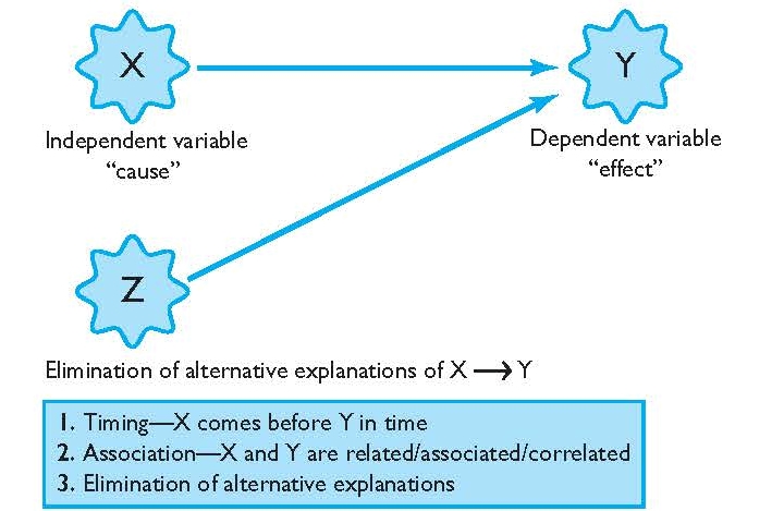
Timing The first condition for a causal relationship is timing. For a causal relationship to exist, it must be shown that the independent variable or cause (X) preceded the dependent variable or outcome (Y) in time. A decrease in domestic violence re-arrests (Y) cannot occur before participation in a domestic violence reduction program (X ), if the domestic violence program is proposed to be the cause of fewer re-arrests. Ensuring that cause comes before effect is not sufficient to establish that a causal relationship exists, but it is one requirement that must be met for a causal relationship.

Association In addition to timing, there must also be an observable association between X and Y, the second necessary condition for a causal relationship. Association is also commonly referred to as covariance or correlation. When an association or correlation exits, this means there is some pattern of relationship between X and Y —as X changes by increasing or decreasing, Y also changes by increasing or decreasing. Here, the notion of X and Y increasing or decreasing can mean an actual increase/decrease in the quantity of some factor, such as an increase/decrease in the number of prison terms or days in a program or re-arrests. It can also refer to an increase/decrease in a particular category, for example, from nonparticipation in a program to participation in a program. For instance, subjects who participated in a domestic violence reduction program (X) incurred fewer domestic violence re-arrests (Y) than those who did not participate in the program. In this example, X and Y are associated—as X change s or increases from nonparticipation to participation in the domestic violence program, Y or the number of re-arrests for domestic violence decreases.

Associations between X and Y can occur in two different directions: positive or negative. A positive association means that as X increases, Y increases, or, as X decreases, Y decreases. A negative association means that as X increases, Y decreases, or, as X decreases, Y increases. In the example above, the association is negative—participation in the domestic violence program was associated with a reduction in re-arrests. This is also sometimes called an inverse relationship.

Elimination of Alternative Explanations Although participation in a domestic violence program may be associated with a reduction in re-arrests, this does not mean for certain that participation in the program was the cause of reduced re-arrests. Just as timing by itself does not imply a causal relationship, association by itself does not imply a causal relationship. For example, instead of the program being the cause of a reduction in re-arrests, perhaps several of the program participants died shortly after completion of the domestic violence program and thus were not able to engage in domestic violence (and their deaths were unknown to the researcher tracking re-arrests). Perhaps a number of the program participants moved out of state and domestic violence re-arrests occurred but were not able to be uncovered by the researcher. Perhaps those in the domestic violence program experienced some other event, such as the trauma of a natural disaster, and that experience led to a reduction in domestic violence, an event not connected to the domestic violence program. If any of these situations occurred, it might appear that the domestic violence program led to fewer re-arrests. However, the observed reduction in re-arrests can actually be attributed to a factor unrelated to the domestic violence program.

The previous discussion leads to the third and final necessary consideration in determining a causal relationship— elimination of alternative explanations. This means that the researcher must rule out any other potential explanation of the results, except for the experimental condition such as a program, policy, or practice. Accounting for or ruling out alternative explanations is much more difficult than ensuring timing and association. Ruling out all alternative explanations is difficult because there are so many potential other explanations that can wholly or partly explain the findings of a research study. This is especially true in the social sciences, where researchers are often interested in relationships explaining human behavior. Because of this difficulty, associations by themselves are sometimes mistaken as causal relationships when in fact they are spurious. A spurious relationship is one where it appears that X and Y are causally related, but the relationship is actually explained by something other than the independent variable, or X.

One only needs to go so far as the daily newspaper to find headlines and stories of mere associations being mistaken, assumed, or represented as causal relationships. For example, a newspaper headline recently proclaimed “Churchgoers live longer.” 3 An uninformed consumer may interpret this headline as evidence of a causal relationship—that going to church by itself will lead to a longer life—but the astute consumer would note possible alternative explanations. For example, people who go to church may live longer because they tend to live healthier lifestyles and tend to avoid risky situations. These are two probable alternative explanations to the relationship independent of simply going to church. In another example, researchers David Kalist and Daniel Yee explored the relationship between first names and delinquent behavior in their manuscript titled “First Names and Crime: Does Unpopularity Spell Trouble?” 4 Kalist and Lee (2009) found that unpopular names are associated with juvenile delinquency. In other words, those individuals with the most unpopular names were more likely to be delinquent than those with more popular names. According to the authors, is it not necessarily someone’s name that leads to delinquent behavior, but rather, the most unpopular names also tend to be correlated with individuals who come from disadvantaged home environments and experience a low socio-economic status of living. Rightly noted by the authors, these alternative explanations help to explain the link between someone’s name and delinquent behavior—a link that is not causal.

A frequently cited example provides more insight to the claim that an association by itself is not sufficient to prove causality. In certain cities in the United States, for example, as ice cream sales increase on a particular day or in a particular month so does the incidence of certain forms of crime. If this association were represented as a causal statement, it would be that ice cream or ice cream sales causes crime. There is an association, no doubt, and let us assume that ice cream sales rose before the increase in crime (timing). Surely, however, this relationship between ice cream sales and crime is spurious. The alternative explanation is that ice cream sales and crime are associated in certain parts of the country because of the weather. Ice cream sales tend to increase in warmer temperatures, and it just so happens that certain forms of crime tend to increase in warmer temperatures as well. This coincidence or association does not mean a causal relationship exists. Additionally, this does not mean that warm temperatures cause crime either. There are plenty of other alternative explanations for the increase in certain forms of crime and warmer temperatures. 6 For another example of a study subject to alternative explanations, read the June 2011 news article titled “Less Crime in U.S. Thanks to Videogames.” 7 Based on your reading, what are some other potential explanations for the crime drop other than videogames?

The preceding examples demonstrate how timing and association can be present, but the final needed condition for a causal relationship is that all alternative explanations are ruled out. While this task is difficult, the classic experimental design helps to ensure these additional explanatory factors are minimized. When other designs are used, such as quasi-experimental designs, the chance that alternative explanations emerge is greater. This potential should become clearer as we explore the organization and logic of the classic experimental design.

CLASSICS IN CJ RESEARCH

Minneapolis Domestic Violence Experiment

The Minneapolis Domestic Violence Experiment (MDVE) 5

Which police action (arrest, separation, or mediation) is most effective at deterring future misdemeanor domestic violence?

The experiment began on March 17, 1981, and continued until August 1, 1982. The experiment was conducted in two of Minneapolis’s four police precincts—the two with the highest number of domestic violence reports and arrests. A total of 314 reports of misdemeanor domestic violence were handled by the police during this time frame.

This study utilized an experimental design with the random assignment of police actions. Each police officer involved in the study was given a pad of report forms. Upon a misdemeanor domestic violence call, the officer’s action (arrest, separation, or mediation) was predetermined by the order and color of report forms in the officer’s notebook. Colored report forms were randomly ordered in the officer’s notebook and the color on the form determined the officer response once at the scene. For example, after receiving a call for domestic violence, an officer would turn to his or her report pad to determine the action. If the top form was pink, the action was arrest. If on the next call the top form was a different color, an action other than arrest would occur. All colored report forms were randomly ordered through a lottery assignment method. The result is that all police officer actions to misdemeanor domestic violence calls were randomly assigned. To ensure the lottery procedure was properly carried out, research staff participated in ride-alongs with officers to ensure that officers did not skip the order of randomly ordered forms. Research staff also made sure the reports were received in the order they were randomly assigned in the pad of report forms.

To examine the relationship of different officer responses to future domestic violence, the researchers examined official arrests of the suspects in a 6-month follow-up period. For example, the researchers examined those initially arrested for misdemeanor domestic violence and how many were subsequently arrested for domestic violence within a 6-month time frame. They did the same procedure for the police actions of separation and mediation. The researchers also interviewed the victim(s) of each incident and asked if a repeat domestic violence incident occurred with the same suspect in the 6-month follow-up period. This allowed researchers to examine domestic violence offenses that may have occurred but did not come to the official attention of police. The researchers then compared official arrests for domestic violence to self-reported domestic violence after the experiment.

Suspects arrested for misdemeanor domestic violence, as opposed to situations where separation or mediation was used, were significantly less likely to engage in repeat domestic violence as measured by official arrest records and victim interviews during the 6-month follow-up period. According to official police records, 10% of those initially arrested engaged in repeat domestic violence in the followup period, 19% of those who initially received mediation engaged in repeat domestic violence, and 24% of those who randomly received separation engaged in repeat domestic violence. According to victim interviews, 19% of those initially arrested engaged in repeat domestic violence, compared to 37% for separation and 33% for mediation. The general conclusion of the experiment was that arrest was preferable to separation or mediation in deterring repeat domestic violence across both official police records and victim interviews.

A few issues that affected the random assignment procedure occurred throughout the study. First, some officers did not follow the randomly assigned action (arrest, separation, or mediation) as a result of other circumstances that occurred at the scene. For example, if the randomly assigned action was separation, but the suspect assaulted the police officer during the call, the officer might arrest the suspect. Second, some officers simply ignored the assigned action if they felt a particular call for domestic violence required another action. For example, if the action was mediation as indicated by the randomly assigned report form, but the officer felt the suspect should be arrested, he or she may have simply ignored the randomly assigned response and substituted his or her own. Third, some officers forgot their report pads and did not know the randomly assigned course of action to take upon a call of domestic violence. Fourth and finally, the police chief also allowed officers to deviate from the randomly assigned action in certain circumstances. In all of these situations, the random assignment procedures broke down.

The results of the MDVE had a rapid and widespread impact on law enforcement practice throughout the United States. Just two years after the release of the study, a 1986 telephone survey of 176 urban police departments serving cities with populations of 100,000 or more found that 46 percent of the departments preferred to make arrests in cases of minor domestic violence, largely due to the effectiveness of this practice in the Minneapolis Domestic Violence Experiment. 8

In an attempt to replicate the findings of the Minneapolis Domestic Violence Experiment, the National Institute of Justice sponsored the Spouse Assault Replication Program. Replication studies were conducted in Omaha, Charlotte, Milwaukee, Miami, and Colorado Springs from 1986–1991. In three of the five replications, offenders randomly assigned to the arrest group had higher levels of continued domestic violence in comparison to other police actions during domestic violence situations. 9 Therefore, rather than providing results that were consistent with the Minneapolis Domestic Violence Experiment, the results from the five replication experiments produced inconsistent findings about whether arrest deters domestic violence. 10

Despite the findings of the replications, the push to arrest domestic violence offenders has continued in law enforcement. Today many police departments require officers to make arrests in domestic violence situations. In agencies that do not mandate arrest, department policy typically states a strong preference toward arrest. State legislatures have also enacted laws impacting police actions regarding domestic violence. Twenty-one states have mandatory arrest laws while eight have pro-arrest statutes for domestic violence. 11

The Classic Experimental Design

Table 5.1 provides an illustration of the classic experimental design. 12 It is important to become familiar with the specific notation and organization of the classic experiment before a full discussion of its components and their purpose.

Major Components of the Classic Experimental Design

The classic experimental design has four major components:

1. Treatment

2. Experimental Group and Control Group

3. Pre-Test and Post-Test

4. Random Assignment

Treatment The first component of the classic experimental design is the treatment, and it is denoted by X in the classic experimental design. The treatment can be a number of things—a program, a new drug, or the implementation of a new policy. In a classic experimental design, the primary goal is to determine what effect, if any, a particular treatment had on some outcome. In this way, the treatment can also be considered the independent variable.

TABLE 5.1 | The Classic Experimental Design

Experimental Group = Group that receives the treatment

Control Group = Group that does not receive the treatment

R = Random assignment

O 1 = Observation before the treatment, or the pre-test

X = Treatment or the independent variable

O 2 = Observation after the treatment, or the post-test

Experimental and Control Groups The second component of the classic experiment is an experimental group and a control group. The experimental group receives the treatment, and the control group does not receive the treatment. There will always be at least one group that receives the treatment in experimental and quasi-experimental designs. In some cases, experiments may have multiple experimental groups receiving multiple treatments.

Pre-Test and Post-Test The third component of the classic experiment is a pre-test and a post-test. A pretest is a measure of the dependent variable or outcome before the treatment. The post-test is a measure of the dependent variable after the treatment is administered. It is important to note that the post-test is defined based on the stated goals of the program. For example, if the stated goal of a particular program is to reduce re-arrests, the post-test will be a measure of re-arrests after the program. The dependent variable also defines the pre-test. For example, if a researcher wanted to examine the impact of a domestic violence reduction program (treatment or X) on the goal of reducing re-arrests (dependent variable or Y), the pre-test would be the number of domestic violence arrests incurred before the program. Program goals may be numerous and all can constitute a post-test, and hence, the pre-test. For example, perhaps the goal of the domestic violence program is also that participants learn of different pro-social ways to handle domestic conflicts other than resorting to violence. If researchers wanted to examine this goal, the post-test might be subjects’ level of knowledge about pro-social ways to handle domestic conflicts other than violence. The pre-test would then be subjects’ level of knowledge about these pro-social alternatives to violence before they received the treatment program.

Although all designs have a post-test, it is not always the case that designs have a pre-test. This is because researchers may not have access or be able to collect information constituting the pre-test. For example, researchers may not be able to determine subjects’ level of knowledge about alternatives to domestic violence before the intervention program if the subjects are already enrolled in the domestic violence intervention program. In other cases, there may be financial barriers to collecting pre-test information. In the teen court evaluation that started this chapter, for example, researchers were not able to collect pre-test information on study participants due to the financial strain it would have placed on the agencies involved in the study. 13 There are a number of potential reasons why a pre-test might not be available in a research study. The defining feature, however, is that the pre-test is determined by the post-test.

Random Assignment The fourth component of the classic experiment is random assignment. Random assignment refers to a process whereby members of the experimental group and control group are assigned to the two groups through a random and unbiased process. Random assignment should not be mistaken for random selection as discussed in Chapter 3. Random selection refers to selecting a smaller but representative sample from a larger population. For example, a researcher may randomly select a sample from a larger city population for the purposes of sending sample members a mail survey to determine their attitudes on crime. The goal of random selection in this example is to make sure the sample, although smaller in size than the population, accurately represents the larger population.

Random assignment, on the other hand, refers to the process of assigning subjects to either the experimental or control group with the goal that the groups are similar or equivalent to each other in every way (see Figure 5.2). The exception to this rule is that one group gets the treatment and the other does not (see discussion below on why equivalence is so important). Although the concept of random is similar in each, the goals are different between random selection and random assignment. 14 Experimental designs all feature random assignment, but this is not true of other research designs, in particular quasi-experimental designs.

FIGURE 5.2 | Random Assignment

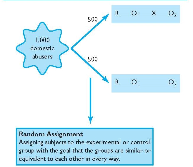
The classic experimental design is the foundation for all other experimental and quasi-experimental designs because it retains all of the major components discussed above. As mentioned, sometimes designs do not have a pre-test, a control group, or random assignment. Because the pre-test, control group, and random assignment are so critical to the goal of uncovering a causal relationship, if one exists, we explore them further below.

The Logic of the Classic Experimental Design

Consider a research study using the classic experimental design where the goal is to determine if a domestic violence treatment program has any effect on re-arrests for domestic violence. The randomly assigned experimental and control groups are comprised of persons who had previously been arrested for domestic violence. The pretest is a measure of the number of domestic violence arrests before the program. This is because the goal of the program is to determine whether re-arrests are impacted after the treatment. The post-test is the number of re-arrests following the treatment program.

Once randomly assigned, the experimental group members receive the domestic violence program, and the control group members do not. After the program, the researcher will compare the pre-test arrests for domestic violence of the experimental group to post-test arrests for domestic violence to determine if arrests increased, decreased, or remained constant since the start of the program. The researcher will also compare the post-test re-arrests for domestic violence between the experimental and control groups. With this example, we explore the usefulness of the classic experimental design, and the contribution of the pre-test, random assignment, and the control group to the goal of determining whether a domestic violence program reduces re-arrests.

The Pre-Test As a component of the classic experiment, the pre-test allows an examination of change in the dependent variable from before the domestic violence program to after the domestic violence program. In short, a pre-test allows the researcher to determine if re-arrests increased, decreased, or remained the same following the domestic violence program. Without a pre-test, researchers would not be able to determine the extent of change, if any, from before to after the program for either the experimental or control group.

Although the pre-test is a measure of the dependent variable before the treatment, it can also be thought of as a measure whereby the researcher can compare the experimental group to the control group before the treatment is administered. For example, the pre-test helps researchers to make sure both groups are similar or equivalent on previous arrests for domestic violence. The importance of equivalence between the experimental and control groups on previous arrests is discussed below with random assignment.

Random Assignment Random assignment helps to ensure that the experimental and control groups are equivalent before the introduction of the treatment. This is perhaps one of the most critical aspects of the classic experiment and all experimental designs. Although the experimental and control groups will be made up of different people with different characteristics, assigning them to groups via a random assignment process helps to ensure that any differences or bias between the groups is eliminated or minimized. By minimizing bias, we mean that the groups will balance each other out on all factors except the treatment. If they are balanced out on all factors prior to the administration of the treatment, any differences between the groups at the post-test must be due to the treatment—the only factor that differs between the experimental group and the control group. According to Shadish, Cook, and Campbell: “If implemented correctly, random assignment creates two or more groups of units that are probabilistically similar to each other on the average. Hence, any outcome differences that are observed between those groups at the end of a study are likely to be due to treatment, not to differences between the groups that already existed at the start of the study.” 15 Considered in another way, if the experimental and control group differed significantly on any relevant factor other than the treatment, the researcher would not know if the results observed at the post-test are attributable to the treatment or to the differences between the groups.

Consider an example where 500 domestic abusers were randomly assigned to the experimental group and 500 were randomly assigned to the control group. Because they were randomly assigned, we would likely find more frequent domestic violence arrestees in both groups, older and younger arrestees in both groups, and so on. If random assignment was implemented correctly, it would be highly unlikely that all of the experimental group members were the most serious or frequent arrestees and all of the control group members were less serious and/or less frequent arrestees. While there are no guarantees, we know the chance of this happening is extremely small with random assignment because it is based on known probability theory. Thus, except for a chance occurrence, random assignment will result in equivalence between the experimental and control group in much the same way that flipping a coin multiple times will result in heads approximately 50% of the time and tails approximately 50% of the time. Over 1,000 tosses of a coin, for example, should result in roughly 500 heads and 500 tails. While there is a chance that flipping a coin 1,000 times will result in heads 1,000 times, or some other major imbalance between heads and tails, this potential is small and would only occur by chance.

The same logic from above also applies with randomly assigning people to groups, and this can even be done by flipping a coin. By assigning people to groups through a random and unbiased process, like flipping a coin, only by chance (or researcher error) will one group have more of one characteristic than another, on average. If there are no major (also called statistically significant) differences between the experimental and control group before the treatment, the most plausible explanation for the results at the post-test is the treatment.

As mentioned, it is possible by some chance occurrence that the experimental and control group members are significantly different on some characteristic prior to administration of the treatment. To confirm that the groups are in fact similar after they have been randomly assigned, the researcher can examine the pre-test if one is present. If the researcher has additional information on subjects before the treatment is administered, such as age, or any other factor that might influence post-test results at the end of the study, he or she can also compare the experimental and control group on those measures to confirm that the groups are equivalent. Thus, a researcher can confirm that the experimental and control groups are equivalent on information known to the researcher.

Being able to compare the groups on known measures is an important way to ensure the random assignment process “worked.” However, perhaps most important is that randomization also helps to ensure similarity across unknown variables between the experimental and control group. Because random assignment is based on known probability theory, there is a much higher probability that all potential differences between the groups that could impact the post-test should balance out with random assignment—known or unknown. Without random assignment, it is likely that the experimental and control group would differ on important but unknown factors and such differences could emerge as alternative explanations for the results. For example, if a researcher did not utilize random assignment and instead took the first 500 domestic abusers from an ordered list and assigned them to the experimental group and the last 500 domestic abusers and assigned them to the control group, one of the groups could be “lopsided” or imbalanced on some important characteristic that could impact the outcome of the study. With random assignment, there is a much higher likelihood that these important characteristics among the experimental and control groups will balance out because no individual has a different chance of being placed into one group versus the other. The probability of one or more characteristics being concentrated into one group and not the other is extremely small with random assignment.

To further illustrate the importance of random assignment to group equivalence, suppose the first 500 domestic violence abusers who were assigned to the experimental group from the ordered list had significantly fewer domestic violence arrests before the program than the last 500 domestic violence abusers on the list. Perhaps this is because the ordered list was organized from least to most chronic domestic abusers. In this instance, the control group would be lopsided concerning number of pre-program domestic violence arrests—they would be more chronic than the experimental group. The arrest imbalance then could potentially explain the post-test results following the domestic violence program. For example, the “less risky” offenders in the experimental group might be less likely to be re-arrested regardless of their participation in the domestic violence program, especially compared to the more chronic domestic abusers in the control group. Because of imbalances between the experimental and control group on arrests before the program was implemented, it would not be known for certain whether an observed reduction in re-arrests after the program for the experimental group was due to the program or the natural result of having less risky offenders in the experimental group. In this instance, the results might be taken to suggest that the program significantly reduces re-arrests. This conclusion might be spurious, however, for the association may simply be due to the fact that the offenders in the experimental group were much different (less frequent offenders) than the control group. Here, the program may have had no effect—the experimental group members may have performed the same regardless of the treatment because they were low-level offenders.

The example above suggests that differences between the experimental and control groups based on previous arrest records could have a major impact on the results of a study. Such differences can arise with the lack of random assignment. If subjects were randomly assigned to the experimental and control group, however, there would be a much higher probability that less frequent and more frequent domestic violence arrestees would have been found in both the experimental and control groups and the differences would have balanced out between the groups—leaving any differences between the groups at the post-test attributable to the treatment only.

In summary, random assignment helps to ensure that the experimental and control group members are balanced or equivalent on all factors that could impact the dependent variable or post-test—known or unknown. The only factor they are not balanced or equal on is the treatment. As such, random assignment helps to isolate the impact of the treatment, if any, on the post-test because it increases confidence that the only difference between the groups should be that one group gets the treatment and the other does not. If that is the only difference between the groups, any change in the dependent variable between the experimental and control group must be attributed to the treatment and not an alternative explanation, such as significant arrest history imbalance between the groups (refer to Figure 5.2). This logic also suggests that if the experimental group and control group are imbalanced on any factor that may be relevant to the outcome, that factor then becomes a potential alternative explanation for the results—an explanation that reduces the researcher’s ability to isolate the real impact of the treatment.

WHAT RESEARCH SHOWS: IMPACTING CRIMINAL JUSTICE OPERATIONS

Scared Straight

The 1978 documentary Scared Straight introduced to the public the “Lifer’s Program” at Rahway State Prison in New Jersey. This program sought to decrease juvenile delinquency by bringing at-risk and delinquent juveniles into the prison where they would be “scared straight” by inmates serving life sentences. Participants in the program were talked to and yelled at by the inmates in an effort to scare them. It was believed that the fear felt by the participants would lead to a discontinuation of their problematic behavior so that they would not end up in prison themselves. Although originally touted as a success based on anecdotal evidence, subsequent evaluations of the program and others like it proved otherwise.

Using a classic experimental design, Finckenauer evaluated the original “Lifer’s Program” at Rahway State Prison. 16 Participating juveniles were randomly assigned to the experimental group or the control group. Results of the evaluation were not positive. Post-test measures revealed that juveniles who were assigned to the experimental group and participated in the program were actually more seriously delinquent afterwards than those who did not participate in the program. Also using an experimental design with random assignment, Yarborough evaluated the “Juvenile Offenders Learn Truth” (JOLT) program at the State Prison of Southern Michigan at Jackson. 17 This program was similar to that of the “Lifer’s Program” only with fewer obscenities used by the inmates. Post-test measurements were taken at two intervals, 3 and 6 months after program completion. Again, results were not positive. Findings revealed no significant differences between those juveniles who attended the program and those who did not.

Other experiments conducted on Scared Straight -like programs further revealed their inability to deter juveniles from future criminality. 18 Despite the intuitive popularity of these programs, these evaluations proved that such programs were not successful. In fact, it is postulated that these programs may have actually done more harm than good.

The Control Group The presence of an equivalent control group (created through random assignment) also gives the researcher more confidence that the findings at the post-test are due to the treatment and not some other alternative explanation. This logic is perhaps best demonstrated by considering how interpretation of results is affected without a control group. Absent an equivalent control group, it cannot be known whether the results of the study are due to the program or some other factor. This is because the control group provides a baseline of comparison or a “control.” For example, without a control group, the researcher may find that domestic violence arrests declined from pre-test to post-test. But the researcher would not be able to definitely attribute that finding to the program without a control group. Perhaps the single experimental group incurred fewer arrests because they matured over their time in the program, regardless of participation in the domestic violence program. Having a randomly assigned control group would allow this consideration to be eliminated, because the equivalent control group would also have naturally matured if that was the case.

Because the control group is meant to be similar to the experimental group on all factors with the exception that the experimental group receives the treatment, the logic is that any differences between the experimental and control group after the treatment must then be attributable only to the treatment itself—everything else occurs equally in both the experimental and control groups and thus cannot be the cause of results. The bottom line is that a control group allows the researcher more confidence to attribute any change in the dependent variable from pre- to post-test and between the experimental and control groups to the treatment—and not another alternative explanation. Absent a control group, the researcher would have much less confidence in the results.

Knowledge about the major components of the classic experimental design and how they contribute to an understanding of cause and effect serves as an important foundation for studying different types of experimental and quasi-experimental designs and their organization. A useful way to become familiar with the components of the experimental design and their important role is to consider the impact on the interpretation of results when one or more components are lacking. For example, what if a design lacked a pre-test? How could this impact the interpretation of post-test results and knowledge about the comparability of the experimental and control group? What if a design lacked random assignment? What are some potential problems that could occur and how could those potential problems impact interpretation of results? What if a design lacked a control group? How does the absence of an equivalent control group affect a researcher’s ability to determine the unique effects of the treatment on the outcomes being measured? The ability to discuss the contribution of a pre-test, random assignment, and a control group—and what is the impact when one or more of those components is absent from a research design—is the key to understanding both experimental and quasi-experimental designs that will be discussed in the remainder of this chapter. As designs lose these important parts and transform from a classic experiment to another experimental design or to a quasi-experiment, they become less useful in isolating the impact that a treatment has on the dependent variable and allow more room for alternative explanations of the results.

One more important point must be made before further delving into experimental and quasi-experimental designs. This point is that rarely, if ever, will the average consumer of research be exposed to the symbols or specific language of the classic experiment, or other experimental and quasi-experimental designs examined in this chapter. In fact, it is unlikely that the average consumer will ever be exposed to the terms pre-test, post-test, experimental group, or random assignment in the popular media, among other terms related to experimental and quasi-experimental designs. Yet, consumers are exposed to research results produced from these and other research designs every day. For example, if a national news organization or your regional newspaper reported a story about the effectiveness of a new drug to reduce cholesterol or the effects of different diets on weight loss, it is doubtful that the results would be reported as produced through a classic experimental design that used a control group and random assignment. Rather, these media outlets would use generally nonscientific terminology such as “results of an experiment showed” or “results of a scientific experiment indicated” or “results showed that subjects who received the new drug had greater cholesterol reductions than those who did not receive the new drug.” Even students who regularly search and read academic articles for use in course papers and other projects will rarely come across such design notation in the research studies they utilize. Depiction of the classic experimental design, including a discussion of its components and their function, simply illustrates the organization and notation of the classic experimental design. Unfortunately, the average consumer has to read between the lines to determine what type of design was used to produce the reported results. Understanding the key components of the classic experimental design allows educated consumers of research to read between those lines.

RESEARCH IN THE NEWS

“Swearing Makes Pain More Tolerable” 19

In 2009, Richard Stephens, John Atkins, and Andrew Kingston of the School of Psychology at Keele University conducted a study with 67 undergraduate students to determine if swearing affects an individual’s response to pain. Researchers asked participants to immerse their hand in a container filled with ice-cold water and repeat a preferred swear word. The researchers then asked the same participants to immerse their hand in ice-cold water while repeating a word used to describe a table (a non-swear word). The results showed that swearing increased pain tolerance compared to the non-swearing condition. Participants who used a swear word were able to hold their hand in ice-cold water longer than when they did not swear. Swearing also decreased participants’ perception of pain.

1. This study is an example of a repeated measures design. In this form of experimental design, study participants are exposed to an experimental condition (swearing with hand in ice-cold water) and a control condition (non-swearing with hand in ice-cold water) while repeated outcome measures are taken with each condition, for example, the length of time a participant was able to keep his or her hand submerged in ice-cold water. Conduct an Internet search for “repeated measures design” and explore the various ways such a study could be conducted, including the potential benefits and drawbacks to this design.

2. After researching repeated measures designs, devise a hypothetical repeated measures study of your own.

3. Retrieve and read the full research study “Swearing as a Response to Pain” by Stephens, Atkins, and Kingston while paying attention to the design and methods (full citation information for this study is listed below). Has your opinion of the study results changed after reading the full study? Why or why not?

Full Study Source: Stephens, R., Atkins, J., and Kingston, A. (2009). “Swearing as a response to pain.” NeuroReport 20, 1056–1060.

Variations on the Experimental Design

The classic experimental design is the foundation upon which all experimental and quasi-experimental designs are based. As such, it can be modified in numerous ways to fit the goals (or constraints) of a particular research study. Below are two variations of the experimental design. Again, knowledge about the major components of the classic experiment, how they contribute to an explanation of results, and what the impact is when one or more components are missing provides an understanding of all other experimental designs.

Post-Test Only Experimental Design

The post-test only experimental design could be used to examine the impact of a treatment program on school disciplinary infractions as measured or operationalized by referrals to the principal’s office (see Table 5.2). In this design, the researcher randomly assigns a group of discipline problem students to the experimental group and control group by flipping a coin—heads to the experimental group and tails to the control group. The experimental group then enters the 3-month treatment program. After the program, the researcher compares the number of referrals to the principal’s office between the experimental and control groups over some period of time, for example, discipline referrals at 6 months after the program. The researcher finds that the experimental group has a much lower number of referrals to the principal’s office in the 6 month follow-up period than the control group.

TABLE 5.2 | Post-Test Only Experimental Design

Several issues arise in this example study. The researcher would not know if discipline problems decreased, increased, or stayed the same from before to after the treatment program because the researcher did not have a count of disciplinary referrals prior to the treatment program (e.g., a pre-test). Although the groups were randomly assigned and are presumed equivalent, the absence of a pre-test means the researcher cannot confirm that the experimental and control groups were equivalent before the treatment was administered, particularly on the number of referrals to the principal’s office. The groups could have differed by a chance occurrence even with random assignment, and any such differences between the groups could potentially explain the post-test difference in the number of referrals to the principal’s office. For example, if the control group included much more serious or frequent discipline problem students than the experimental group by chance, this difference might explain the lower number of referrals for the experimental group, not that the treatment produced this result.

Experimental Design with Two Treatments and a Control Group

This design could be used to determine the impact of boot camp versus juvenile detention on post-release recidivism (see Table 5.3). Recidivism in this study is operationalized as re-arrest for delinquent behavior. First, a population of known juvenile delinquents is randomly assigned to either boot camp, juvenile detention, or a control condition where they receive no sanction. To accomplish random assignment to groups, the researcher places the names of all youth into a hat and assigns the groups in order. For example, the first name pulled goes into experimental group 1, the next into experimental group 2, and the next into the control group, and so on. Once randomly assigned, the experimental group youth receive either boot camp or juvenile detention for a period of 3 months, whereas members of the control group are released on their own recognizance to their parents. At the end of the experiment, the researcher compares the re-arrest activity of boot camp participants to detention delinquents to control group members during a 6-month follow-up period.

TABLE 5.3 | Experimental Design with Two Treatments and a Control Group

This design has several advantages. First, it includes all major components of the classic experimental design, and simply adds an additional treatment for comparison purposes. Random assignment was utilized and this means that the groups have a higher probability of being equivalent on all factors that could impact the post-test. Thus, random assignment in this example helps to ensure the only differences between the groups are the treatment conditions. Without random assignment, there is a greater chance that one group of youth was somehow different, and this difference could impact the post-test. For example, if the boot camp youth were much less serious and frequent delinquents than the juvenile detention youth or control group youth, the results might erroneously show that the boot camp reduced recidivism when in fact the youth in boot camp may have been the “best risks”—unlikely to get re-arrested with or without boot camp. The pre-test in the example above allows the researcher to determine change in re-arrests from pretest to post-test. Thus, the researcher can determine if delinquent behavior, as measured by re-arrest, increased, decreased, or remained constant from pre- to post-test. The pre-test also allows the researcher to confirm that the random assignment process resulted in equivalent groups based on the pre-test. Finally, the presence of a control group allows the researcher to have more confidence that any differences in the post-test are due to the treatment. For example, if the control group had more re-arrests than the boot camp or juvenile detention experimental groups 6 months after their release from those programs, the researcher would have more confidence that the programs produced fewer re-arrests because the control group members were the same as the experimental groups; the only difference was that they did not receive a treatment.

The one key feature of experimental designs is that they all retain random assignment. This is why they are considered “experimental” designs. Sometimes, however, experimental designs lack a pre-test. Knowledge of the usefulness of a pre-test demonstrates the potential problems with those designs where it is missing. For example, in the post-test only experimental design, a researcher would not be able to make a determination of change in the dependent variable from pre- to post-test. Perhaps most importantly, the researcher would not be able to confirm that the experimental and control groups were in fact equivalent on a pre-test measure before the introduction of the treatment. Even though both groups were randomly assigned, and probability theory suggests they should be equivalent, without a pre-test measure the researcher could not confirm similarity because differences could occur by chance even with random assignment. If there were any differences at the post-test between the experimental group and control group, the results might be due to some explanation other than the treatment, namely that the groups differed prior to the administration of the treatment. The same limitation could apply in any form of experimental design that does not utilize a pre-test for conformational purposes.

Understanding the contribution of a pre-test to an experimental design shows that it is a critical component. It provides a measure of change and also gives the researcher more confidence that the observed results are due to the treatment, and not some difference between the experimental and control groups. Despite the usefulness of a pre-test, however, perhaps the most critical ingredient of any experimental design is random assignment. It is important to note that all experimental designs retain random assignment.

Experimental Designs Are Rare in Criminal Justice and Criminology

The classic experiment is the foundation for other types of experimental and quasi-experimental designs. The unfortunate reality, however, is that the classic experiment, or other experimental designs, are few and far between in criminal justice. 20 Recall that one of the major components of an experimental design is random assignment. Achieving random assignment is often a barrier to experimental research in criminal justice. Achieving random assignment might, for example, require the approval of the chief (or city council or both) of a major metropolitan police agency to allow researchers to randomly assign patrol officers to certain areas of a city and/or randomly assign police officer actions. Recall the MDVE. This experiment required the full cooperation of the chief of police and other decision-makers to allow researchers to randomly assign police actions. In another example, achieving random assignment might require a judge to randomly assign a group of youthful offenders to a certain juvenile court sanction (experimental group), and another group of similar youthful offenders to no sanction or an alternative sanction as a control group. 21 In sum, random assignment typically requires the cooperation of a number of individuals and sometimes that cooperation is difficult to obtain.

Even when random assignment can be accomplished, sometimes it is not implemented correctly and the random assignment procedure breaks down. This is another barrier to conducting experimental research. For example, in the MDVE, researchers randomly assigned officer responses, but the officers did not always follow the assigned course of action. Moreover, some believe that the random assignment of criminal justice programs, sentences, or randomly assigning officer responses may be unethical in certain circumstances, and even a violation of the rights of citizens. For example, some believe it is unfair when random assignment results in some delinquents being sentenced to boot camp while others get assigned to a control group without any sanction at all or a less restrictive sanction than boot camp. In the MDVE, some believe it is unfair that some suspects were arrested and received an official record whereas others were not arrested for the same type of behavior. In other cases, subjects in the experimental group may receive some benefit from the treatment that is essentially denied to the control group for a period of time and this can become an issue as well.

There are other important reasons why random assignment is difficult to accomplish. Random assignment may, for example, involve a disruption of the normal procedures of agencies and their officers. In the MDVE, officers had to adjust their normal and established routine, and this was a barrier at times in that study. Shadish, Cook, and Campbell also note that random assignment may not always be feasible or desirable when quick answers are needed. 22 This is because experimental designs sometimes take a long time to produce results. In addition to the time required in planning and organizing the experiment, and treatment delivery, researchers may need several months if not years to collect and analyze the data before they have answers. This is particularly important because time is often of the essence in criminal justice research, especially in research efforts testing the effect of some policy or program where it is not feasible to wait years for answers. Waiting for the results of an experimental design means that many policy-makers may make decisions without the results.

Quasi-Experimental Designs

In general terms, quasi-experiments include a group of designs that lack random assignment. Quasi-experiments may also lack other parts, such as a pre-test or a control group, just like some experimental designs. The absence of random assignment, however, is the ingredient that transforms an otherwise experimental design into a quasi-experiment. Lacking random assignment is a major disadvantage because it increases the chances that the experimental and control groups differ on relevant factors before the treatment—both known and unknown—differences that may then emerge as alternative explanations of the outcomes.

Just like experimental designs, quasi-experimental designs can be organized in many different ways. This section will discuss three types of quasi-experiments: nonequivalent group design, one-group longitudinal design, and two-group longitudinal design.

Nonequivalent Group Design

The nonequivalent group design is perhaps the most common type of quasi-experiment. 23 Notice that it is very similar to the classic experimental design with the exception that it lacks random assignment (see Table 5.4). Additionally, what was labeled the experimental group in an experimental design is sometimes called the treatment group in the nonequivalent group design. What was labeled the control group in the experimental design is sometimes called the comparison group in the nonequivalent group design. This terminological distinction is an indicator that the groups were not created through random assignment.

TABLE 5.4 | Nonequivalent Group Design

NR = Not Randomly assigned

One of the main problems with the nonequivalent group design is that it lacks random assignment, and without random assignment, there is a greater chance that the treatment and comparison groups may be different in some way that can impact study results. Take, for example, a nonequivalent group design where a researcher is interested in whether an aggression-reduction treatment program can reduce inmate-on-inmate assaults in a prison setting. Assume that the researcher asked for inmates who had previously been involved in assaultive activity to volunteer for the aggression-reduction program. Suppose the researcher placed the first 50 volunteers into the treatment group and the next 50 volunteers into the comparison group. Note that this method of assignment is not random but rather first come, first serve.

Because the study utilized volunteers and there was no random assignment, it is possible that the first 50 volunteers placed into the treatment group differed significantly from the last 50 volunteers who were placed in the comparison group. This can lead to alternative explanations for the results. For example, if the treatment group was much younger than the comparison group, the researcher may find at the end of the program that the treatment group still maintained a higher rate of infractions than the comparison group—even after the aggression-reduction program! The conclusion might be that the aggression program actually increased the level of violence among the treatment group. This conclusion would likely be spurious and may be due to the age differential between the treatment and comparison groups. Indeed, research has revealed that younger inmates are significantly more likely to engage in prison assaults than older inmates. The fact that the treatment group incurred more assaults than the comparison group after the aggression-reduction program may only relate to the age differential between the groups, not that the program had no effect or that it somehow may have increased aggression. The previous example highlights the importance of random assignment and the potential problems that can occur in its absence.

Although researchers who utilize a quasi-experimental design are not able to randomly assign their subjects to groups, they can employ other techniques in an attempt to make the groups as equivalent as possible on known or measured factors before the treatment is given. In the example above, it is likely that the researcher would have known the age of inmates, their prior assault record, and various other pieces of information (e.g., previous prison stays). Through a technique called matching, the researcher could make sure the treatment and comparison groups were “matched” on these important factors before administering the aggression reduction program to the treatment group. This type of matching can be done individual to individual (e.g., subject #1 in treatment group is matched to a selected subject #1 in comparison group on age, previous arrests, gender), or aggregately, such that the comparison group is similar to the treatment group overall (e.g., average ages between groups are similar, equal proportions of males and females). Knowledge of these and other important variables, for example, would allow the researcher to make sure that the treatment group did not have heavy concentrations of younger or more frequent or serious offenders than the comparison group—factors that are related to assaultive activity independent of the treatment program. In short, matching allows the researcher some control over who goes into the treatment and comparison groups so as to balance these groups on important factors absent random assignment. If unbalanced on one or more factors, these factors could emerge as alternative explanations of the results. Figure 5.3 demonstrates the logic of matching both at the individual and aggregate level in a quasi-experimental design.

Matching is an important part of the nonequivalent group design. By matching, the researcher can approximate equivalence between the groups on important variables that may influence the post-test. However, it is important to note that a researcher can only match subjects on factors that they have information about—a researcher cannot match the treatment and comparison group members on factors that are unmeasured or otherwise unknown but which may still impact outcomes. For example, if the researcher has no knowledge about the number of previous incarcerations, the researcher cannot match the treatment and comparison groups on this factor. Matching also requires that the information used for matching is valid and reliable, which is not always the case. Agency records, for example, are notorious for inconsistencies, errors, omissions, and for being dated, but are often utilized for matching purposes. Asking survey questions to generate information for matching (for example, how many times have you been incarcerated?) can also be problematic because some respondents may lie, forget, or exaggerate their behavior or experiences.

In addition to the above considerations, the more factors a researcher wishes to match the group members on, the more difficult it becomes to find appropriate matches. Matching on prior arrests or age is less complex than matching on several additional pieces of information. Finally, matching is never considered superior to random assignment when the goal is to construct equitable groups. This is because there is a much higher likelihood of equivalence with random assignment on factors that are both measured and unknown to the researcher. Thus, the results produced from a nonequivalent group design, even with matching, are at a greater risk of alternative explanations than an experimental design that features random assignment.

FIGURE 5.3 | (a) Individual Matching (b) Aggregate Matching

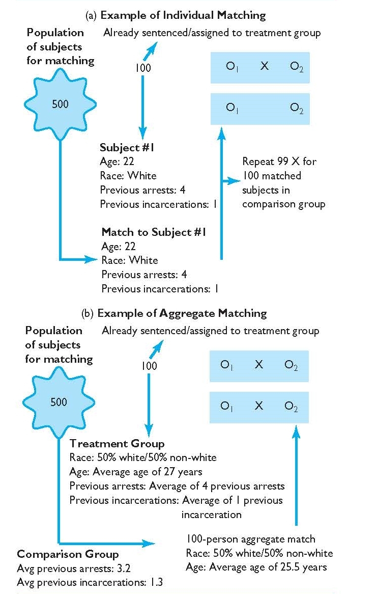
The previous discussion is not to suggest that the nonequivalent group design cannot be useful in answering important research questions. Rather, it is to suggest that the nonequivalent group design, and hence any quasi-experiment, is more susceptible to alternative explanations than the classic experimental design because of the absence of random assignment. As a result, a researcher must be prepared to rule out potential alternative explanations. Quasi-experimental designs that lack a pre-test or a comparison group are even less desirable than the nonequivalent group design and are subject to additional alternative explanations because of these missing parts. Although the quasi-experiment may be all that is available and still can serve as an important design in evaluating the impact of a particular treatment, it is not preferable to the classic experiment. Researchers (and consumers) must be attuned to the potential issues of this design so as to make informed conclusions about the results produced from such research studies.

The Effects of Red Light Camera (RLC) Enforcement

On March 15, 2009, an article appeared in the Santa Cruz Sentinel entitled “Ticket’s in the Mail: Red-Light Cameras Questioned.” The article stated “while studies show fewer T-bone crashes at lights with cameras and fewer drivers running red lights, the number of rear-end crashes increases.” 24 The study mentioned in the newspaper, which showed fewer drivers running red lights with cameras, was conducted by Richard Retting, Susan Ferguson, and Charles Farmer of the Insurance Institute for Highway Safety (IIHS). 25 They completed a quasi-experimental study in Philadelphia to determine the impact of red light cameras (RLC) on red light violations. In the study, the researchers selected nine intersections—six of which were experimental sites that utilized RLCs and three comparison sites that did not utilize RLCs. The six experimental sites were located in Philadelphia, Pennsylvania, and the three comparison sites were located in Atlantic County, New Jersey. The researchers chose the comparison sites based on the proximity to Philadelphia, the ability to collect data using the same methods as at experimental intersections (e.g., the use of cameras for viewing red light traffic), and the fact that police officials in Atlantic County had offered assistance selecting and monitoring the intersections.

The authors collected three phases of information in the RLC study at the experimental and comparison sites:

Phase 1 Data Collection: Baseline (pre-test) data collection at the experimental and comparison sites consisting of the number of vehicles passing through each intersection, the number of red light violations, and the rate of red light violations per 10,000 vehicles.

Phase 2 Data Collection: Number of vehicles traveling through experimental and comparison intersections, number of red light violations after a 1-second yellow light increase at the experimental sites (treatment 1), number of red light violations at comparison sites without a 1-second yellow light increase, and red light violations per 10,000 vehicles at both experimental and comparison sites.

Phase 3 Data Collection: Red light violations after a 1-second yellow light increase and RLC enforcement at the experimental sites (treatment 2), red light violations at comparison sites without a 1-second yellow increase or RLC enforcement, number of vehicles passing through the experimental and comparison intersections, and the rate of red light violations per 10,000 vehicles.

The researchers operationalized “red light violations” as those where the vehicle entered the intersection one-half of a second or more after the onset of the red signal where the vehicle’s rear tires had to be positioned behind the crosswalk or stop line prior to entering on red. Vehicles already in the intersection at the onset of the red light, or those making a right turn on red with or without stopping were not considered red light violations.

The researchers collected video data at each of the experimental and comparison sites during Phases 1–3. This allowed the researchers to examine red light violations before, during, and after the implementation of red light enforcement and yellow light time increases. Based on an analysis of data, the researchers revealed that the implementation of a 1-second yellow light increase led to reductions in the rate of red light violations from Phase 1 to Phase 2 in all of the experimental sites. In 2 out of 3 comparison sites, the rate of red light violations also decreased, despite no yellow light increase. From Phase 2 to Phase 3 (the enforcement of red light camera violations in addition to a 1-second yellow light increase at experimental sites), the authors noted decreases in the rate of red light violations in all experimental sites, and decreases among 2 of 3 comparison sites without red light enforcement in effect.

Concluding their study, the researchers noted that the study “found large and highly significant incremental reductions in red light running associated with increased yellow signal timing followed by the introduction of red light cameras.” Despite these findings, the researchers noted a number of potential factors to consider in light of the findings: the follow-up time periods utilized when counting red light violations before and after the treatment conditions were instituted; publicity about red light camera enforcement; and the size of fines associated with red light camera enforcement (the fine in Philadelphia was $100, higher than in many other cities), among others.

After reading about the study used in the newspaper article, has your impression of the newspaper headline and quote changed?

For more information and research on the effect of RLCs, visit the Insurance Institute for Highway Safety at http://www .iihs.org/research/topics/rlr.html .

One-Group Longitudinal Design

Like all experimental designs, the quasi-experimental design can come in a variety of forms. The second quasi-experimental design (above) is the one-group longitudinal design (also called a simple interrupted time series design). 26 An examination of this design shows that it lacks both random assignment and a comparison group (see Table 5.5). A major difference between this design and others we have covered is that it includes multiple pre-test and post-test observations.

TABLE 5.5 | One-Group Longitudinal Design

The one-group longitudinal design is useful when researchers are interested in exploring longer-term patterns. Indeed, the term longitudinal generally means “over time”—repeated measurements of the pre-test and post-test over time. This is different from cross-sectional designs, which examine the pre-test and post-test at only one point in time (e.g., at a single point before the application of the treatment and at a single point after the treatment). For example, in the nonequivalent group design and the classic experimental design previously examined, both are cross-sectional because pre-tests and post-tests are measured at one point in time (e.g., at a point 6 months after the treatment). Yet, these designs could easily be considered longitudinal if researchers took repeated measures of the pre-test and post-test.

The organization of the one-group longitudinal design is to examine a baseline of several pre-test observations, introduce a treatment or intervention, and then examine the post-test at several different time intervals. As organized, this design is useful for gauging the impact that a particular program, policy, or law has, if any, and how long the treatment impact lasts. Consider an example whereby a researcher is interested in gauging the impact of a tobacco ban on inmate-on-inmate assaults in a prison setting. This is an important question, for recent years have witnessed correctional systems banning all tobacco products from prison facilities. Correctional administrators predicted that there would be a major increase of inmate-on-inmate violence once the bans took effect. The one-group longitudinal design would be one appropriate design to examine the impact of banning tobacco on inmate assaults.

To construct this study using the one-group longitudinal design, the researcher would first examine the rate of inmate-on-inmate assaults in the prison system (or at an individual prison, a particular cellblock, or whatever the unit of analysis) prior to the removal of tobacco. This is the pre-test, or a baseline of assault activity before the ban goes into effect. In the design presented above, perhaps the researcher would measure the level of assaults in the preceding four months prior to the tobacco ban. When establishing a pre-test baseline, the general rule is that, in a longitudinal design, the more time utilized, both in overall time and number of intervals, the better. For example, the rate of assaults in the preceding month is not as useful as an entire year of data on inmate assaults prior to the tobacco ban. Next, once the tobacco ban is implemented, the researcher would then measure the rate of inmate assaults in the coming months to determine what impact the ban had on inmate-on-inmate assaults. This is shown in Table 5.5 as the multiple post-test measures of assaults. Assaults may increase, decrease, or remain constant from the pre-test baseline over the term of the post-test.

If assaults increased at the same time as the ban went into effect, the researcher might conclude that the increase was due only to the tobacco ban. But, could there be alternative explanations? The answer to this question is yes, there may be other plausible explanations for the increase even with several months of pre-test data. Unfortunately, without a comparison group there is no way for the researcher to be certain if the increase in assaults was due to the tobacco ban, or some other factor that may have spurred the increase in assaults and happened at the same time as the tobacco ban. What if assaults decreased after the tobacco ban went into effect? In this scenario, because there is no comparison group, the researcher would still not know if the results would have happened anyway without the tobacco ban. In these instances, the lack of a comparison group prevents the researcher from confidently attributing the results to the tobacco ban, and interpretation is subject to numerous alternative explanations.

Two-Group Longitudinal Design

A remedy for the previous situation would be to introduce a comparison group (see Table 5.6). Prior to the full tobacco ban, suppose prison administrators conducted a pilot program at one prison to provide insight as to what would happen once the tobacco ban went into effect systemwide. To conduct this pilot, the researcher identified one prison. At this prison, the researcher identified two different cellblocks, C-Block and D-Block. C-Block constitutes the treatment group, or the cellblock of inmates who will have their tobacco taken away. D-Block is the comparison group—inmates in this cellblock will retain their tobacco privileges during the course of the study and during a determined follow-up period to measure post-test assaults (e.g., 12-months). This is a two-group longitudinal design (also sometimes called a multiple interrupted time series design), and adding a comparison group makes this design superior to the one-group longitudinal design.

TABLE 5.6 | Two-Group Longitudinal Design

The usefulness of adding a comparison group to the study means that the researcher can have more confidence that the results at the post-test are due to the tobacco ban and not some alternative explanation. This is because any difference in assaults at the post-test between the treatment and comparison group should be attributed to the only difference between them, the tobacco ban. For this interpretation to hold, however, the researcher must be sure that C-Block and D-Block are similar or equivalent on all factors that might influence the post-test. There are many potential factors that should be considered. For example, the researcher will want to make sure that the same types of inmates are housed in both cellblocks. If a chronic group of assaultive inmates constitutes members of C-Block, but not D-Block, this differential could explain the results, not the treatment.

The researcher might also want to make sure equitable numbers of tobacco and non-tobacco users are found in each cellblock. If very few inmates in C-Block are smokers, the real effect of removing tobacco may be hidden. The researcher might also examine other areas where potential differences might arise, for example, that both cellblocks are staffed with equal numbers of officers, that officers in each cellblock tend to resolve inmate disputes similarly, and other potential issues that could influence post-test measure of assaults. Equivalence could also be ensured by comparing the groups on additional evidence before the ban takes effect: number of prior prison sentences, time served in prison, age, seriousness of conviction crime, and other factors that might relate to assaultive behavior, regardless of the tobacco ban. Moreover, the researcher should ensure that inmates in C-Block do not know that their D-Block counterparts are still allowed tobacco during the pilot study, and vice versa. If either group knows about the pilot program being an experiment, they might act differently than normal, and this could become an explanation of results. Additionally, the researchers might also try to make sure that C-Block inmates are completely tobacco free after the ban goes into effect—that they do not hoard, smuggle, or receive tobacco from officers or other inmates during the tobacco ban in or outside of the cellblock. If these and other important differences are accounted for at the individual and cellblock level, the researcher will have more confidence that any differences in assaults at the post-test between the treatment and comparison groups are related to the tobacco ban, and not some other difference between the two groups or the two cellblocks.

The addition of a comparison group aids in the ability of the researcher to isolate the true impact of a tobacco ban on inmate-on-inmate assaults. All factors that influence the treatment group should also influence the comparison group because the groups are made up of equivalent individuals in equivalent circumstances, with the exception of the tobacco ban. If this is the only difference, the results can be attributed to the ban. Although the addition of the comparison group in the two-group longitudinal design provides more confidence that the findings are attributed to the tobacco ban, the fact that this design lacks randomization means that alternative explanations cannot be completely ruled out—but they can be minimized. This example also suggests that the quasi-experiment in this instance may actually be preferable to an experimental design—noting the realities of prison administration. For example, prison inmates are not typically randomly assigned to different cellblocks by prison officers. Moreover, it is highly unlikely that a prison would have two open cellblocks waiting for a researcher to randomly assign incoming inmates to the prison for a tobacco ban study. Therefore, it is likely there would be differences among the groups in the quasi-experiment.

Fortunately, if differences between the groups are present, the researcher can attempt to determine their potential impact before interpretation of results. The researcher can also use statistical models after the ban takes effect to determine the impact of any differences between the groups on the post-test. While the two-group longitudinal quasi-experiment just discussed could also take the form of an experimental design, if random assignment could somehow be accomplished, the previous discussion provides one situation where an experimental design might be appropriate and desired for a particular research question, but would not be realistic considering the many barriers.

The Threat of Alternative Explanations

Alternative explanations are those factors that could explain the post-test results, other than the treatment. Throughout this chapter, we have noted the potential for alternative explanations and have given several examples of explanations other than the treatment. It is important to know that potential alternative explanations can arise in any research design discussed in this chapter. However, alternative explanations often arise because some design part is missing, for example, random assignment, a pre-test, or a control or comparison group. This is especially true in criminal justice where researchers often conduct field studies and have less control over their study conditions than do researchers who conduct experiments under highly controlled laboratory conditions. A prime example of this is the tobacco ban study, where it would be difficult for researchers to ensure that C-Block inmates, the treatment group, were completely tobacco free during the course of the study.

Alternative explanations are typically referred to as threats to internal validity. In this context, if an experiment is internally valid, it means that alternative explanations have been ruled out and the treatment is the only factor that produced the results. If a study is not internally valid, this means that alternative explanations for the results exist or potentially exist. In this section, we focus on some common alternative explanations that may arise in experimental and quasi-experimental designs. 27

Selection Bias

One of the more common alternative explanations that may occur is selection bias. Selection bias generally indicates that the treatment group (or experimental group) is somehow different from the comparison group (or control group) on a factor that could influence the post-test results. Selection bias is more often a threat in quasi-experimental designs than experimental designs due to the lack of random assignment. Suppose in our study of the prison tobacco ban, members of C-Block were substantially younger than members of D-Block, the comparison group. Such an imbalance between the groups would mean the researcher would not know if the differences in assaults are real (meaning the result of the tobacco ban) or a result of the age differential. Recall that research shows that younger inmates are more assaultive than older inmates and so we would expect more assaults among the younger offenders independent of the tobacco ban.

In a quasi-experiment, selection bias is perhaps the most prevalent type of alternative explanation and can seriously compromise results. Indeed, many of the examples above have referred to potential situations where the groups are imbalanced or not equivalent on some important factor. Although selection bias is a common threat in quasi-experimental designs because of lack of random assignment, and can be a threat in experimental designs because the groups could differ by chance alone or the practice of randomization was not maintained throughout the study (see Classics in CJ Research-MDVE above), a researcher may be able to detect such differentials. For example, the researcher could detect such differences by comparing the groups on the pre-test or other types of information before the start of the study. If differences were found, the researcher could take measures to correct them. The researcher could also use a statistical model that could account or control for differences between the groups and isolate the impact of the treatment, if any. This discussion is beyond the scope of this text but would be a potential way to deal with selection bias and estimate the impact of this bias on study results. The researcher could also, if possible, attempt to re-match the groups in a quasi-experiment or randomly assign the groups a second time in an experimental design to ensure equivalence. At the least, the researcher could recognize the group differences and discuss their potential impact on the results. Without a pre-test or other pre-study information on study participants, however, such differences might not be able to be detected and, therefore, it would be more difficult to determine how the differences, as a result of selection bias, influenced the results.

Another potential alternative explanation is history. History refers to any event experienced differently by the treatment and comparison groups in the time between the pre-test and the post-test that could impact results. Suppose during the course of the tobacco ban study several riots occurred on D-Block, the comparison group. Because of the riots, prison officers “locked down” this cellblock numerous times. Because D-Block inmates were locked down at various times, this could have affected their ability to otherwise engage in inmate assaults. At the end of the study, the assaults in D-Block might have decreased from their pre-test levels because of the lockdowns, whereas in C-Block assaults may have occurred at their normal pace because there was not a lockdown, or perhaps even increased from the pretest because tobacco was also taken away. Even if the tobacco ban had no effect and assaults remained constant in C-Block from pre- to post-test, the lockdown in D-Block might make it appear that the tobacco ban led to increased assaults in C-Block. Thus, the researcher would not know if the post-test results for the C-Block treatment group were attributable to the tobacco ban or the simple fact that D-Block inmates were locked down and their assault activity was artificially reduced. In this instance, the comparison group becomes much less useful because the lockdown created a historical factor that imbalanced the groups during the treatment phase and nullified the comparison.

Another potential alternative explanation is maturation. Maturation refers to the natural biological, psychological, or emotional processes we all experience as time passes—aging, becoming more or less intelligent, becoming bored, and so on. For example, if a researcher was interested in the effect of a boot camp on recidivism for juvenile offenders, it is possible that over the course of the boot camp program the delinquents naturally matured as they aged and this produced the reduction in recidivism—not that the boot camp somehow led to this reduction. This threat is particularly applicable in situations that deal with populations that rapidly change over a relatively short period of time or when a treatment lasts a considerable period of time. However, this threat could be eliminated with a comparison group that is similar to the treatment group. This is because the maturation effects would occur in both groups and the effect of the boot camp, if any, could be isolated. This assumes, however, that the groups are matched and equitable on factors subject to the maturation process, such as age. If not, such differentials could be an alternative explanation of results. For example, if the treatment and comparison groups differ by age, on average, this could mean that one group changes or matures at a different rate than the other group. This differential rate of change or maturation as a result of the age differential could explain the results, not the treatment. This example demonstrates how selection bias and maturation can interact at the same time as alternative explanations. This example also suggests the importance of an equivalent control or comparison group to eliminate or minimize the impact of maturation as an alternative explanation.

Attrition or Subject Mortality

Attrition or subject mortality is another typical alternative explanation. Attrition refers to differential loss in the number or type of subjects between the treatment and comparison groups and can occur in both experimental and quasi-experimental designs. Suppose we wanted to conduct a study to determine who is the better research methods professor among the authors of this textbook. Let’s assume that we have an experimental design where students were randomly assigned to professor 1, professor 2, or professor 3. By randomly assigning students to each respective professor, there is greater probability that the groups are equivalent and thus there are no differences between the three groups with one exception—the professor they receive and his or her particular teaching and delivery style. This is the treatment. Let’s also assume that the professors will be administering the same tests and using the same textbook. After the group members are randomly assigned, a pre-treatment evaluation shows the groups are in fact equivalent on all important known factors that could influence post-test scores, such as grade point average, age, time in school, and exposure to research methods concepts. Additionally, all groups scored comparably on a pre-test of knowledge about research methods, thus there is more confidence that the groups are in fact equivalent.

At the conclusion of the study, we find that professor 2’s group has the lowest final test scores of the three. However, because professor 2 is such an outstanding professor, the results appear odd. At first glance, the researcher thinks the results could have been influenced by students dropping out of the class. For example, perhaps several of professor 2’s students dropped the course but none did from the classes of professor 1 or 3. It is revealed, however, that an equal number of students dropped out of all three courses before the post-test and, therefore, this could not be the reason for the low scores in professor 2’s course. Upon further investigation, however, the researcher finds that although an equal number of students dropped out of each class, the dropouts in professor 2’s class were some of his best students. In contrast, those who dropped out of professor 1’s and professor 3’s courses were some of their poorest students. In this example, professor 2 appears to be the least effective teacher. However, this result appears to be due to the fact that his best students dropped out, and this highly influenced the final test average for his group. Although there was not a differential loss of subjects in terms of numbers (which can also be an attrition issue), there was differential loss in the types of students. This differential loss, not the teaching style, is an alternative explanation of the results.

Testing or Testing Bias

Another potential alternative explanation is testing or testing bias. Suppose that after the pre-test of research methods knowledge, professor 1 and professor 3 reviewed the test with their students and gave them the correct answers. Professor 2 did not. The fact that professor l’s and professor 3’s groups did better on the post-test final exam may be explained by the finding that students in those groups remembered the answers to the pre-test, were thus biased at the pre-test, and this artificially inflated their post-test scores. Testing bias can explain the results because students in groups 1 and 3 may have simply remembered the answers from the pre-test review. In fact, the students in professor l’s and 3’s courses may have scored high on the post-test without ever having been exposed to the treatment because they were biased at the pre-test.

Instrumentation

Another alternative explanation that can arise is instrumentation. Instrumentation refers to changes in the measuring instrument from pre- to post-test. Using the previous example, suppose professors 1 and 3 did not give the same final exam as professor 2. For example, professors 1 and 3 changed the final exam and professor 2 kept the final exam the same as the pretest. Because professors 1 and 3 changed the exam, and perhaps made it easier or somehow different from the pre-test exam, results that showed lower scores for professor 2’s students may be related only to instrumentation changes from pre- to post-test. Obviously, to limit the influence of instrumentation, researchers should make sure that instruments remain consistent from pre- to post-test.

A final alternative explanation is reactivity. Reactivity occurs when members of the treatment or experimental group change their behavior simply as a result of being part of a study. This is akin to the finding that people tend to change their behavior when they are being watched or are aware they are being studied. If members of the experiment know they are part of an experiment and are being studied and watched, it is possible that their behavior will change independent of the treatment. If this occurs, the researcher will not know if the behavior change is the result of the treatment, or simply a result of being part of a study. For example, suppose a researcher wants to determine if a boot camp program impacts the recidivism of delinquent offenders. Members of the experimental group are sentenced to boot camp and members of the control group are released on their own recognizance to their parents. Because members of the experimental group know they are part of the experiment, and hence being watched closely after they exit boot camp, they may artificially change their behavior and avoid trouble. Their change of behavior may be totally unrelated to boot camp, but rather, to their knowledge of being part of an experiment.

Other Potential Alternative Explanations

The above discussion provided some typical alternative explanations that may arise with the designs discussed in this chapter. There are, however, other potential alternative explanations that may arise. These alternative explanations arise only when a control or comparison group is present.

One such alternative explanation is diffusion of treatment. Diffusion of treatment occurs when the control or comparison group learns about the treatment its members are being denied and attempts to mimic the behavior of the treatment group. If the control group is successful in mimicking the experimental group, for example, the results at the end of the study may show similarity in outcomes between groups and cause the researcher to conclude that the program had no effect. In fact, however, the finding of no effect can be explained by the comparison group mimicking the treatment group. 28 In reality, there may be no effect of the treatment, but the researcher would not know this for sure because the control group effectively transformed into another experimental group—there is then no baseline of comparison. Consider a study where a researcher wants to determine the impact of a training program on class behavior and participation. In this study, the experimental group is exposed to several sessions of training on how to act appropriately in class and how to engage in class participation. The control group does not receive such training, but they are aware that they are part of an experiment. Suppose after a few class sessions the control group starts to mimic the behavior of the experimental group, acting the same way and participating in class the same way. At the conclusion of the study, the researcher might determine that the program had no impact because the comparison group, which did not receive the new program, showed similar progress.

In a related explanation, sometimes the comparison or control group learns about the experiment and attempts to compete with the experimental or treatment group. This alternative explanation is called compensatory rivalry. For example, suppose a police chief wants to determine if a new training program will increase the endurance of SWAT team officers. The chief randomly assigns SWAT members to either an experimental or control group. The experimental group will receive the new endurance training program and the control group will receive the normal program that has been used for years. During the course of the study, suppose the control group learns that the treatment group is receiving the new endurance program and starts to compete with the experimental group. Perhaps the control group runs five more miles per day and works out an extra hour in the weight room, in addition to their normal endurance program. At the end of the study, and due to the control group’s extra and competing effort, the results might show no effect of the new endurance program, and at worst, experimental group members may show a decline in endurance compared to the control group. The rivalry or competing behavior actually explains the results, not that the new endurance program has no effect or a damaging effect. Although the new endurance program may in reality have no effect, this cannot be known because of the actions of the control group, who learned about the treatment and competed with the experimental group.

Closely related to compensatory rivalry is the alternative explanation of comparison or control group demoralization. 29 In this instance, instead of competing with the experimental or treatment group, the control or comparison group simply gives up and changes their normal behavior. Using the SWAT example, perhaps the control group simply quits their normal endurance program when they learn about the treatment group receiving the new endurance program. At the post-test, their endurance will likely drop considerably compared to the treatment group. Because of this, the new endurance program might emerge as a shining success. In reality, however, the researcher will not know if any changes in endurance between the experimental and control groups are a result of the new endurance program or the control group giving up. Due to their giving up, there is no longer a comparison group of equitable others, the change in endurance among the treatment group members could be attributed to a number of alternative explanations, for example, maturation. If the comparison group behaves normally, the researcher will be able to exclude maturation as a potential explanation. This is because any maturation effects will occur in both groups.

The previous discussion suggests that when the control or comparison group learns about the experiment and the treatment they are denied, potential alternative explanations can arise. Perhaps the best remedy to protect from the alternative explanations just discussed is to make sure the treatment and comparison groups do not have contact with one another. In laboratory experiments this can be ensured, but sometimes this is a problem in criminal justice studies, which are often conducted in the field.

The previous discussion also suggests that there are numerous alternative explanations that can impact the interpretation of results from a study. A careful researcher would know that alternative explanations must be ruled out before reaching a definitive conclusion about the impact of a particular program. The researcher must be attuned to these potential alternative explanations because they can influence results and how results are interpreted. Moreover, the discussion shows that several alternative explanations can occur at the same time. For example, it is possible that selection bias, maturation, attrition, and compensatory rivalry all emerge as alternative explanations in the same study. Knowing about these potential alternative explanations and how they can impact the results of a study is what distinguishes a consumer of research from an educated consumer of research.

Chapter Summary

The primary focus of this chapter was the classic experimental design, the foundation for other types of experimental and quasi-experimental designs. The classic experimental design is perhaps the most useful design when exploring causal relationships. Often, however, researchers cannot employ the classic experimental design to answer a research question. In fact, the classic experimental design is rare in criminal justice and criminology because it is often difficult to ensure random assignment for a variety of reasons. In circumstances where an experimental design is appropriate but not feasible, researchers may turn to one of many quasi-experimental designs. The most important difference between the two is that quasi-experimental designs do not feature random assignment. This can create potential problems for researchers. The main problem is that there is a greater chance the treatment and comparison groups may differ on important characteristics that could influence the results of a study. Although researchers can attempt to prevent imbalances between the groups by matching them on important known characteristics, it is still much more difficult to establish equivalence than it is in the classic experiment. As such, it becomes more difficult to determine what impact a treatment had, if any, as one moves from an experimental to a quasi-experimental design.

Perhaps the most important lesson to be learned in this chapter is that to be an educated consumer of research results requires an understanding of the type of design that produced the results. There are numerous ways experimental and quasi-experimental designs can be structured. This is why much attention was paid to the classic experimental design. In reality, all experimental and quasi-experimental designs are variations of the classic experiment in some way—adding or deleting certain components. If the components and organization and logic of the classic experimental design are understood, consumers of research will have a better understanding of the results produced from any sort of research design. For example, what problems in interpretation arise when a design lacks a pre-test, a control group, or random assignment? Having an answer to this question is a good start toward being an informed consumer of research results produced through experimental and quasi-experimental designs.

Critical Thinking Questions

1. Why is randomization/random assignment preferable to matching? Provide several reasons with explanation.

2. What are some potential reasons a researcher would not be able to utilize random assignment?

3. What is a major limitation of matching?

4. What is the difference between a longitudinal study and a cross-sectional study?

5. Describe a hypothetical study where maturation, and not the treatment, could explain the outcomes of the research.

association (or covariance or correlation): One of three conditions that must be met for establishing cause and effect, or a causal relationship. Association refers to the condition that X and Y must be related for a causal relationship to exist. Association is also referred to as covariance or correlation. Although two variables may be associated (or covary or be correlated), this does not automatically imply that they are causally related

attrition or subject mortality: A threat to internal validity, it refers to the differential loss of subjects between the experimental (treatment) and control (comparison) groups during the course of a study

cause and effect relationship: A cause and effect relationship occurs when one variable causes another, and no other explanation for that relationship exists

classic experimental design or experimental design: A design in a research study that features random assignment to an experimental or control group. Experimental designs can vary tremendously, but a constant feature is random assignment, experimental and control groups, and a post-test. For example, a classic experimental design features random assignment, a treatment, experimental and control groups, and pre- and post-tests

comparison group: The group in a quasi-experimental design that does not receive the treatment. In an experimental design, the comparison group is referred to as the control group

compensatory rivalry: A threat to internal validity, it occurs when the control or comparison group attempts to compete with the experimental or treatment group

control group: In an experimental design, the control group does not receive the treatment. The control group serves as a baseline of comparison to the experimental group. It serves as an example of what happens when a group equivalent to the experimental group does not receive the treatment

cross-sectional designs: A measurement of the pre-test and post-test at one point in time (e.g., six months before and six months after the program)

demoralization: A threat to internal validity closely associated with compensatory rivalry, it occurs when the control or comparison group gives up and changes their normal behavior. While in compensatory rivalry the group members compete, in demoralization, they simply quit. Both are not normal behavioral reactions

dependent variable: Also known as the outcome in a research study. A post-test is a measure of the dependent variable

diffusion of treatment: A threat to internal validity, it occurs when the control or comparison group members learn that they are not getting the treatment and attempt to mimic the behavior of the experimental or treatment group. This mimicking may make it seem as if the treatment is having no effect, when in fact it may be

elimination of alternative explanations: One of three conditions that must be met for establishing cause and effect. Elimination of alternative explanations means that the researcher has ruled out other explanations for an observed relationship between X and Y

experimental group: In an experimental design, the experimental group receives the treatment

history: A threat to internal validity, it refers to any event experienced differently by the treatment and comparison groups—an event that could explain the results other than the supposed cause

independent variable: Also called the cause

instrumentation: A threat to internal validity, it refers to changes in the measuring instrument from pre- to post-test

longitudinal: Refers to repeated measurements of the pre-test and post-test over time, typically for the same group of individuals. This is the opposite of cross-sectional

matching: A process sometimes utilized in some quasi-experimental designs that feature treatment and comparison groups. Matching is a process whereby the researcher attempts to ensure equivalence between the treatment and comparison groups on known information, in the absence of the ability to randomly assign the groups

maturation: A threat to internal validity, maturation refers to the natural biological, psychological, or emotional processes as time passes

negative association: Refers to a negative association between two variables. A negative association is demonstrated when X increases and Y decreases, or X decreases and Y increases. Also known as an inverse relationship—the variables moving in opposite directions

operationalized or operationalization: Refers to the process of assigning a working definition to a concept. For example, the concept of intelligence can be operationalized or defined as grade point average or score on a standardized exam, among others

pilot program or test: Refers to a smaller test study or pilot to work out problems before a larger study and to anticipate changes needed for a larger study. Similar to a test run

positive association: Refers to a positive association between two variables. A positive association means as X increases, Y increases, or as X decreases, Y decreases

post-test: The post-test is a measure of the dependent variable after the treatment has been administered

pre-test: The pre-test is a measure of the dependent variable or outcome before a treatment is administered

quasi-experiment: A quasi-experiment refers to any number of research design configurations that resemble an experimental design but primarily lack random assignment. In the absence of random assignment, quasi-experimental designs feature matching to attempt equivalence

random assignment: Refers to a process whereby members of the experimental group and control group are assigned to each group through a random and unbiased process

random selection: Refers to selecting a smaller but representative subset from a population. Not to be confused with random assignment

reactivity: A threat to internal validity, it occurs when members of the experimental (treatment) or control (comparison) group change their behavior unnaturally as a result of being part of a study

selection bias: A threat to internal validity, selection bias occurs when the experimental (treatment) group and control (comparison) group are not equivalent. The difference between the groups can be a threat to internal validity, or, an alternative explanation to the findings

spurious: A spurious relationship is one where X and Y appear to be causally related, but in fact the relationship is actually explained by a variable or factor other than X

testing or testing bias: A threat to internal validity, it refers to the potential of study members being biased prior to a treatment, and this bias, rather than the treatment, may explain study results

threat to internal validity: Also known as alternative explanation to a relationship between X and Y. Threats to internal validity are factors that explain Y, or the dependent variable, and are not X, or the independent variable

timing: One of three conditions that must be met for establishing cause and effect. Timing refers to the condition that X must come before Y in time for X to be a cause of Y. While timing is necessary for a causal relationship, it is not sufficient, and considerations of association and eliminating other alternative explanations must be met

treatment: A component of a research design, it is typically denoted by the letter X. In a research study on the impact of teen court on juvenile recidivism, teen court is the treatment. In a classic experimental design, the treatment is given only to the experimental group, not the control group

treatment group: The group in a quasi-experimental design that receives the treatment. In an experimental design, this group is called the experimental group

unit of analysis: Refers to the focus of a research study as being individuals, groups, or other units of analysis, such as prisons or police agencies, and so on

variable(s): A variable is a concept that has been given a working definition and can take on different values. For example, intelligence can be defined as a person’s grade point average and can range from low to high or can be defined numerically by different values such as 3.5 or 4.0

1 Povitsky, W., N. Connell, D. Wilson, & D. Gottfredson. (2008). “An experimental evaluation of teen courts.” Journal of Experimental Criminology, 4, 137–163.

2 Hirschi, T., and H. Selvin (1966). “False criteria of causality in delinquency.” Social Problems, 13, 254–268.

3 Robert Roy Britt, “Churchgoers Live Longer.” April, 3, 2006. http://www.livescience.com/health/060403_church_ good.html. Retrieved on September 30, 2008.

4 Kalist, D., and D. Yee (2009). “First names and crime: Does unpopularity spell trouble?” Social Science Quarterly, 90 (1), 39–48.

5 Sherman, L. (1992). Policing domestic violence. New York: The Free Press.

6 For historical and interesting reading on the effects of weather on crime and other disorder, see Dexter, E. (1899). “Influence of weather upon crime.” Popular Science Monthly, 55, 653–660 in Horton, D. (2000). Pioneering Perspectives in Criminology. Incline Village, NV: Copperhouse.

7 http://www.escapistmagazine.com/news/view/111191-Less-Crime-in-U-S-Thanks-to-Videogames , retrieved on September 13, 2011. This news article was in response to a study titled “Understanding the effects of violent videogames on violent crime.” See Cunningham, Scott, Engelstätter, Benjamin, and Ward, (April 7, 2011). Available at SSRN: http://ssm.com/abstract= 1804959.

8 Cohn, E. G. (1987). “Changing the domestic violence policies of urban police departments: Impact of the Minneapolis experiment.” Response, 10 (4), 22–24.

9 Schmidt, Janell D., & Lawrence W. Sherman (1993). “Does arrest deter domestic violence?” American Behavioral Scientist, 36 (5), 601–610.

10 Maxwell, Christopher D., Joel H. Gamer, & Jeffrey A. Fagan. (2001). The effects of arrest on intimate partner violence: New evidence for the spouse assault replication program. Washington D.C.: National Institute of Justice.

11 Miller, N. (2005). What does research and evaluation say about domestic violence laws? A compendium of justice system laws and related research assessments. Alexandria, VA: Institute for Law and Justice.

12 The sections on experimental and quasi-experimental designs rely heavily on the seminal work of Campbell and Stanley (Campbell, D.T., & J. C. Stanley. (1963). Experimental and quasi-experimental designs for research. Chicago: RandMcNally) and more recently, Shadish, W., T. Cook, & D. Campbell. (2002). Experimental and quasi-experimental designs for generalized causal inference. New York: Houghton Mifflin.

13 Povitsky et al. (2008). p. 146, note 9.

14 Shadish, W., T. Cook, & D. Campbell. (2002). Experimental and quasi-experimental designs for generalized causal inference. New York: Houghton Mifflin Company.

15 Ibid, 15.

16 Finckenauer, James O. (1982). Scared straight! and the panacea phenomenon. Englewood Cliffs, N.J.: Prentice Hall.

17 Yarborough, J.C. (1979). Evaluation of JOLT (Juvenile Offenders Learn Truth) as a deterrence program. Lansing, MI: Michigan Department of Corrections.

18 Petrosino, Anthony, Carolyn Turpin-Petrosino, & James O. Finckenauer. (2000). “Well-meaning programs can have harmful effects! Lessons from experiments of programs such as Scared Straight.” Crime and Delinquency, 46, 354–379.

19 “Swearing makes pain more tolerable” retrieved at http:// www.livescience.com/health/090712-swearing-pain.html (July 13, 2009). Also see “Bleep! My finger! Why swearing helps ease pain” by Tiffany Sharpies, retrieved at http://www.time.com/time/health/article /0,8599,1910691,00.html?xid=rss-health (July 16, 2009).

20 For an excellent discussion of the value of controlled experiments and why they are so rare in the social sciences, see Sherman, L. (1992). Policing domestic violence. New York: The Free Press, 55–74.

21 For discussion, see Weisburd, D., T. Einat, & M. Kowalski. (2008). “The miracle of the cells: An experimental study of interventions to increase payment of court-ordered financial obligations.” Criminology and Public Policy, 7, 9–36.

22 Shadish, Cook, & Campbell. (2002).

24 Kelly, Cathy. (March 15, 2009). “Tickets in the mail: Red-light cameras questioned.” Santa Cruz Sentinel.

25 Retting, Richard, Susan Ferguson, & Charles Farmer. (January 2007). “Reducing red light running through longer yellow signal timing and red light camera enforcement: Results of a field investigation.” Arlington, VA: Insurance Institute for Highway Safety.

26 Shadish, Cook, & Campbell. (2002).

27 See Shadish, Cook, & Campbell. (2002), pp. 54–61 for an excellent discussion of threats to internal validity. Also see Chapter 2 for an extended discussion of all forms of validity considered in research design.

28 Trochim, W. (2001). The research methods knowledge base, 2nd ed. Cincinnati, OH: Atomic Dog.

Applied Research Methods in Criminal Justice and Criminology by University of North Texas is licensed under a Creative Commons Attribution-NonCommercial 4.0 International License , except where otherwise noted.

Share This Book

Want to create or adapt books like this? Learn more about how Pressbooks supports open publishing practices.

Chapter 7: Nonexperimental Research

Quasi-Experimental Research

Learning Objectives

• Explain what quasi-experimental research is and distinguish it clearly from both experimental and correlational research.
• Describe three different types of quasi-experimental research designs (nonequivalent groups, pretest-posttest, and interrupted time series) and identify examples of each one.

The prefix  quasi  means “resembling.” Thus quasi-experimental research is research that resembles experimental research but is not true experimental research. Although the independent variable is manipulated, participants are not randomly assigned to conditions or orders of conditions (Cook & Campbell, 1979). [1] Because the independent variable is manipulated before the dependent variable is measured, quasi-experimental research eliminates the directionality problem. But because participants are not randomly assigned—making it likely that there are other differences between conditions—quasi-experimental research does not eliminate the problem of confounding variables. In terms of internal validity, therefore, quasi-experiments are generally somewhere between correlational studies and true experiments.

Quasi-experiments are most likely to be conducted in field settings in which random assignment is difficult or impossible. They are often conducted to evaluate the effectiveness of a treatment—perhaps a type of psychotherapy or an educational intervention. There are many different kinds of quasi-experiments, but we will discuss just a few of the most common ones here.

Nonequivalent Groups Design

Recall that when participants in a between-subjects experiment are randomly assigned to conditions, the resulting groups are likely to be quite similar. In fact, researchers consider them to be equivalent. When participants are not randomly assigned to conditions, however, the resulting groups are likely to be dissimilar in some ways. For this reason, researchers consider them to be nonequivalent. A  nonequivalent groups design , then, is a between-subjects design in which participants have not been randomly assigned to conditions.

Imagine, for example, a researcher who wants to evaluate a new method of teaching fractions to third graders. One way would be to conduct a study with a treatment group consisting of one class of third-grade students and a control group consisting of another class of third-grade students. This design would be a nonequivalent groups design because the students are not randomly assigned to classes by the researcher, which means there could be important differences between them. For example, the parents of higher achieving or more motivated students might have been more likely to request that their children be assigned to Ms. Williams’s class. Or the principal might have assigned the “troublemakers” to Mr. Jones’s class because he is a stronger disciplinarian. Of course, the teachers’ styles, and even the classroom environments, might be very different and might cause different levels of achievement or motivation among the students. If at the end of the study there was a difference in the two classes’ knowledge of fractions, it might have been caused by the difference between the teaching methods—but it might have been caused by any of these confounding variables.

Of course, researchers using a nonequivalent groups design can take steps to ensure that their groups are as similar as possible. In the present example, the researcher could try to select two classes at the same school, where the students in the two classes have similar scores on a standardized math test and the teachers are the same sex, are close in age, and have similar teaching styles. Taking such steps would increase the internal validity of the study because it would eliminate some of the most important confounding variables. But without true random assignment of the students to conditions, there remains the possibility of other important confounding variables that the researcher was not able to control.

Pretest-Posttest Design

In a  pretest-posttest design , the dependent variable is measured once before the treatment is implemented and once after it is implemented. Imagine, for example, a researcher who is interested in the effectiveness of an antidrug education program on elementary school students’ attitudes toward illegal drugs. The researcher could measure the attitudes of students at a particular elementary school during one week, implement the antidrug program during the next week, and finally, measure their attitudes again the following week. The pretest-posttest design is much like a within-subjects experiment in which each participant is tested first under the control condition and then under the treatment condition. It is unlike a within-subjects experiment, however, in that the order of conditions is not counterbalanced because it typically is not possible for a participant to be tested in the treatment condition first and then in an “untreated” control condition.

If the average posttest score is better than the average pretest score, then it makes sense to conclude that the treatment might be responsible for the improvement. Unfortunately, one often cannot conclude this with a high degree of certainty because there may be other explanations for why the posttest scores are better. One category of alternative explanations goes under the name of  history . Other things might have happened between the pretest and the posttest. Perhaps an antidrug program aired on television and many of the students watched it, or perhaps a celebrity died of a drug overdose and many of the students heard about it. Another category of alternative explanations goes under the name of  maturation . Participants might have changed between the pretest and the posttest in ways that they were going to anyway because they are growing and learning. If it were a yearlong program, participants might become less impulsive or better reasoners and this might be responsible for the change.

Another alternative explanation for a change in the dependent variable in a pretest-posttest design is  regression to the mean . This refers to the statistical fact that an individual who scores extremely on a variable on one occasion will tend to score less extremely on the next occasion. For example, a bowler with a long-term average of 150 who suddenly bowls a 220 will almost certainly score lower in the next game. Her score will “regress” toward her mean score of 150. Regression to the mean can be a problem when participants are selected for further study  because  of their extreme scores. Imagine, for example, that only students who scored especially low on a test of fractions are given a special training program and then retested. Regression to the mean all but guarantees that their scores will be higher even if the training program has no effect. A closely related concept—and an extremely important one in psychological research—is  spontaneous remission . This is the tendency for many medical and psychological problems to improve over time without any form of treatment. The common cold is a good example. If one were to measure symptom severity in 100 common cold sufferers today, give them a bowl of chicken soup every day, and then measure their symptom severity again in a week, they would probably be much improved. This does not mean that the chicken soup was responsible for the improvement, however, because they would have been much improved without any treatment at all. The same is true of many psychological problems. A group of severely depressed people today is likely to be less depressed on average in 6 months. In reviewing the results of several studies of treatments for depression, researchers Michael Posternak and Ivan Miller found that participants in waitlist control conditions improved an average of 10 to 15% before they received any treatment at all (Posternak & Miller, 2001) [2] . Thus one must generally be very cautious about inferring causality from pretest-posttest designs.

Does Psychotherapy Work?

Early studies on the effectiveness of psychotherapy tended to use pretest-posttest designs. In a classic 1952 article, researcher Hans Eysenck summarized the results of 24 such studies showing that about two thirds of patients improved between the pretest and the posttest (Eysenck, 1952) [3] . But Eysenck also compared these results with archival data from state hospital and insurance company records showing that similar patients recovered at about the same rate  without  receiving psychotherapy. This parallel suggested to Eysenck that the improvement that patients showed in the pretest-posttest studies might be no more than spontaneous remission. Note that Eysenck did not conclude that psychotherapy was ineffective. He merely concluded that there was no evidence that it was, and he wrote of “the necessity of properly planned and executed experimental studies into this important field” (p. 323). You can read the entire article here: Classics in the History of Psychology .

Fortunately, many other researchers took up Eysenck’s challenge, and by 1980 hundreds of experiments had been conducted in which participants were randomly assigned to treatment and control conditions, and the results were summarized in a classic book by Mary Lee Smith, Gene Glass, and Thomas Miller (Smith, Glass, & Miller, 1980) [4] . They found that overall psychotherapy was quite effective, with about 80% of treatment participants improving more than the average control participant. Subsequent research has focused more on the conditions under which different types of psychotherapy are more or less effective.

Interrupted Time Series Design

A variant of the pretest-posttest design is the  interrupted time-series design . A time series is a set of measurements taken at intervals over a period of time. For example, a manufacturing company might measure its workers’ productivity each week for a year. In an interrupted time series-design, a time series like this one is “interrupted” by a treatment. In one classic example, the treatment was the reduction of the work shifts in a factory from 10 hours to 8 hours (Cook & Campbell, 1979) [5] . Because productivity increased rather quickly after the shortening of the work shifts, and because it remained elevated for many months afterward, the researcher concluded that the shortening of the shifts caused the increase in productivity. Notice that the interrupted time-series design is like a pretest-posttest design in that it includes measurements of the dependent variable both before and after the treatment. It is unlike the pretest-posttest design, however, in that it includes multiple pretest and posttest measurements.

Figure 7.3 shows data from a hypothetical interrupted time-series study. The dependent variable is the number of student absences per week in a research methods course. The treatment is that the instructor begins publicly taking attendance each day so that students know that the instructor is aware of who is present and who is absent. The top panel of  Figure 7.3 shows how the data might look if this treatment worked. There is a consistently high number of absences before the treatment, and there is an immediate and sustained drop in absences after the treatment. The bottom panel of  Figure 7.3 shows how the data might look if this treatment did not work. On average, the number of absences after the treatment is about the same as the number before. This figure also illustrates an advantage of the interrupted time-series design over a simpler pretest-posttest design. If there had been only one measurement of absences before the treatment at Week 7 and one afterward at Week 8, then it would have looked as though the treatment were responsible for the reduction. The multiple measurements both before and after the treatment suggest that the reduction between Weeks 7 and 8 is nothing more than normal week-to-week variation.

Combination Designs

A type of quasi-experimental design that is generally better than either the nonequivalent groups design or the pretest-posttest design is one that combines elements of both. There is a treatment group that is given a pretest, receives a treatment, and then is given a posttest. But at the same time there is a control group that is given a pretest, does  not  receive the treatment, and then is given a posttest. The question, then, is not simply whether participants who receive the treatment improve but whether they improve  more  than participants who do not receive the treatment.

Imagine, for example, that students in one school are given a pretest on their attitudes toward drugs, then are exposed to an antidrug program, and finally are given a posttest. Students in a similar school are given the pretest, not exposed to an antidrug program, and finally are given a posttest. Again, if students in the treatment condition become more negative toward drugs, this change in attitude could be an effect of the treatment, but it could also be a matter of history or maturation. If it really is an effect of the treatment, then students in the treatment condition should become more negative than students in the control condition. But if it is a matter of history (e.g., news of a celebrity drug overdose) or maturation (e.g., improved reasoning), then students in the two conditions would be likely to show similar amounts of change. This type of design does not completely eliminate the possibility of confounding variables, however. Something could occur at one of the schools but not the other (e.g., a student drug overdose), so students at the first school would be affected by it while students at the other school would not.

Finally, if participants in this kind of design are randomly assigned to conditions, it becomes a true experiment rather than a quasi experiment. In fact, it is the kind of experiment that Eysenck called for—and that has now been conducted many times—to demonstrate the effectiveness of psychotherapy.

Key Takeaways

• Quasi-experimental research involves the manipulation of an independent variable without the random assignment of participants to conditions or orders of conditions. Among the important types are nonequivalent groups designs, pretest-posttest, and interrupted time-series designs.
• Quasi-experimental research eliminates the directionality problem because it involves the manipulation of the independent variable. It does not eliminate the problem of confounding variables, however, because it does not involve random assignment to conditions. For these reasons, quasi-experimental research is generally higher in internal validity than correlational studies but lower than true experiments.
• Practice: Imagine that two professors decide to test the effect of giving daily quizzes on student performance in a statistics course. They decide that Professor A will give quizzes but Professor B will not. They will then compare the performance of students in their two sections on a common final exam. List five other variables that might differ between the two sections that could affect the results.
• regression to the mean
• spontaneous remission

Image Descriptions

Figure 7.3 image description: Two line graphs charting the number of absences per week over 14 weeks. The first 7 weeks are without treatment and the last 7 weeks are with treatment. In the first line graph, there are between 4 to 8 absences each week. After the treatment, the absences drop to 0 to 3 each week, which suggests the treatment worked. In the second line graph, there is no noticeable change in the number of absences per week after the treatment, which suggests the treatment did not work. [Return to Figure 7.3]

• Cook, T. D., & Campbell, D. T. (1979). Quasi-experimentation: Design & analysis issues in field settings . Boston, MA: Houghton Mifflin. ↵
• Posternak, M. A., & Miller, I. (2001). Untreated short-term course of major depression: A meta-analysis of studies using outcomes from studies using wait-list control groups. Journal of Affective Disorders, 66 , 139–146. ↵
• Eysenck, H. J. (1952). The effects of psychotherapy: An evaluation. Journal of Consulting Psychology, 16 , 319–324. ↵
• Smith, M. L., Glass, G. V., & Miller, T. I. (1980). The benefits of psychotherapy . Baltimore, MD: Johns Hopkins University Press. ↵

A between-subjects design in which participants have not been randomly assigned to conditions.

The dependent variable is measured once before the treatment is implemented and once after it is implemented.

A category of alternative explanations for differences between scores such as events that happened between the pretest and posttest, unrelated to the study.

An alternative explanation that refers to how the participants might have changed between the pretest and posttest in ways that they were going to anyway because they are growing and learning.

The statistical fact that an individual who scores extremely on a variable on one occasion will tend to score less extremely on the next occasion.

The tendency for many medical and psychological problems to improve over time without any form of treatment.

A set of measurements taken at intervals over a period of time that are interrupted by a treatment.

Research Methods in Psychology - 2nd Canadian Edition Copyright © 2015 by Paul C. Price, Rajiv Jhangiani, & I-Chant A. Chiang is licensed under a Creative Commons Attribution-NonCommercial-ShareAlike 4.0 International License , except where otherwise noted.

Share This Book

• school Campus Bookshelves
• menu_book Bookshelves
• perm_media Learning Objects
• login Login
• how_to_reg Request Instructor Account
• hub Instructor Commons

Margin Size

• Download Page (PDF)
• Download Full Book (PDF)
• Periodic Table
• Physics Constants
• Scientific Calculator
• Reference & Cite
• Tools expand_more
• Readability

selected template will load here

This action is not available.

12.2: Pre-experimental and quasi-experimental design

• Last updated
• Save as PDF
• Page ID 25667

• Matthew DeCarlo
• Radford University via Open Social Work Education

\( \newcommand{\vecs}[1]{\overset { \scriptstyle \rightharpoonup} {\mathbf{#1}} } \)

\( \newcommand{\vecd}[1]{\overset{-\!-\!\rightharpoonup}{\vphantom{a}\smash {#1}}} \)

\( \newcommand{\id}{\mathrm{id}}\) \( \newcommand{\Span}{\mathrm{span}}\)

( \newcommand{\kernel}{\mathrm{null}\,}\) \( \newcommand{\range}{\mathrm{range}\,}\)

\( \newcommand{\RealPart}{\mathrm{Re}}\) \( \newcommand{\ImaginaryPart}{\mathrm{Im}}\)

\( \newcommand{\Argument}{\mathrm{Arg}}\) \( \newcommand{\norm}[1]{\| #1 \|}\)

\( \newcommand{\inner}[2]{\langle #1, #2 \rangle}\)

\( \newcommand{\Span}{\mathrm{span}}\)

\( \newcommand{\id}{\mathrm{id}}\)

\( \newcommand{\kernel}{\mathrm{null}\,}\)

\( \newcommand{\range}{\mathrm{range}\,}\)

\( \newcommand{\RealPart}{\mathrm{Re}}\)

\( \newcommand{\ImaginaryPart}{\mathrm{Im}}\)

\( \newcommand{\Argument}{\mathrm{Arg}}\)

\( \newcommand{\norm}[1]{\| #1 \|}\)

\( \newcommand{\Span}{\mathrm{span}}\) \( \newcommand{\AA}{\unicode[.8,0]{x212B}}\)

\( \newcommand{\vectorA}[1]{\vec{#1}}      % arrow\)

\( \newcommand{\vectorAt}[1]{\vec{\text{#1}}}      % arrow\)

\( \newcommand{\vectorB}[1]{\overset { \scriptstyle \rightharpoonup} {\mathbf{#1}} } \)

\( \newcommand{\vectorC}[1]{\textbf{#1}} \)

\( \newcommand{\vectorD}[1]{\overrightarrow{#1}} \)

\( \newcommand{\vectorDt}[1]{\overrightarrow{\text{#1}}} \)

\( \newcommand{\vectE}[1]{\overset{-\!-\!\rightharpoonup}{\vphantom{a}\smash{\mathbf {#1}}}} \)

Learning Objectives

• Identify and describe the various types of quasi-experimental designs
• Distinguish true experimental designs from quasi-experimental and pre-experimental designs
• Identify and describe the various types of quasi-experimental and pre-experimental designs

As we discussed in the previous section, time, funding, and ethics may limit a researcher’s ability to conduct a true experiment. For researchers in the medical sciences and social work, conducting a true experiment could require denying needed treatment to clients, which is a clear ethical violation. Even those whose research may not involve the administration of needed medications or treatments may be limited in their ability to conduct a classic experiment. When true experiments are not possible, researchers often use quasi-experimental designs.

Quasi-experimental designs are similar to true experiments, but they lack random assignment to experimental and control groups. The most basic of these quasi-experimental designs is the nonequivalent comparison groups design (Rubin & Babbie, 2017). [1] The nonequivalent comparison group design looks a lot like the classic experimental design, except it does not use random assignment. In many cases, these groups may already exist. For example, a researcher might conduct research at two different agency sites, one of which receives the intervention and the other does not. No one was assigned to treatment or comparison groups. Those groupings existed prior to the study. While this method is more convenient for real-world research, researchers cannot be sure that the groups are comparable. Perhaps the treatment group has a characteristic that is unique–for example, higher income or different diagnoses–that make the treatment more effective.

Quasi-experiments are particularly useful in social welfare policy research. Social welfare policy researchers like me often look for what are termed natural experiments , or situations in which comparable groups are created by differences that already occur in the real world. For example, Stratmann and Wille (2016) [2] were interested in the effects of a state healthcare policy called Certificate of Need on the quality of hospitals. They clearly cannot assign states to adopt one set of policies or another. Instead, researchers used hospital referral regions, or the areas from which hospitals draw their patients, that spanned across state lines. Because the hospitals were in the same referral region, researchers could be pretty sure that the client characteristics were pretty similar. In this way, they could classify patients in experimental and comparison groups without affecting policy or telling people where to live.

There are important examples of policy experiments that use random assignment, including the Oregon Medicaid experiment. In the Oregon Medicaid experiment, the wait list for Oregon was so long, state officials conducted a lottery to see who from the wait list would receive Medicaid (Baicker et al., 2013). [3] Researchers used the lottery as a natural experiment that included random assignment. People selected to be a part of Medicaid were the experimental group and those on the wait list were in the control group. There are some practical complications with using people on a wait list as a control group—most obviously, what happens when people on the wait list are accepted into the program while you’re still collecting data? Natural experiments aren’t a specific kind of experiment like quasi- or pre-experimental designs. Instead, they are more like a feature of the social world that allows researchers to use the logic of experimental design to investigate the connection between variables.

Matching is another approach in quasi-experimental design to assigning experimental and comparison groups. Researchers should think about what variables are important in their study, particularly demographic variables or attributes that might impact their dependent variable. Individual matching involves pairing participants with similar attributes. When this is done at the beginning of an experiment, the matched pair is split—with one participant going to the experimental group and the other to the control group. An ex post facto control group , in contrast, is when a researcher matches individuals after the intervention is administered to some participants. Finally, researchers may engage in aggregate matching , in which the comparison group is determined to be similar on important variables.

There are many different quasi-experimental designs in addition to the nonequivalent comparison group design described earlier. Describing all of them is beyond the scope of this textbook, but one more design is worth mentioning. The time series design uses multiple observations before and after an intervention. In some cases, experimental and comparison groups are used. In other cases where that is not feasible, a single experimental group is used. By using multiple observations before and after the intervention, the researcher can better understand the true value of the dependent variable in each participant before the intervention starts. Additionally, multiple observations afterwards allow the researcher to see whether the intervention had lasting effects on participants. Time series designs are similar to single-subjects designs, which we will discuss in Chapter 15.

When true experiments and quasi-experiments are not possible, researchers may turn to a pre-experimental design (Campbell & Stanley, 1963). [4] Pre-experimental designs are called such because they often happen before a true experiment is conducted. Researchers want to see if their interventions will have some effect on a small group of people before they seek funding and dedicate time to conduct a true experiment. Pre-experimental designs, thus, are usually conducted as a first step towards establishing the evidence for or against an intervention. However, this type of design comes with some unique disadvantages, which we’ll describe as we review the pre-experimental designs available.

If we wished to measure the impact of a natural disaster, such as Hurricane Katrina for example, we might conduct a pre-experiment by identifying an experimental group from a community that experienced the hurricane and a control group from a similar community that had not been hit by the hurricane. This study design, called a static group comparison , has the advantage of including a comparison group that did not experience the stimulus (in this case, the hurricane). Unfortunately, it is difficult to know those groups are truly comparable because the experimental and control groups were determined by factors other than random assignment. Additionally, the design would only allow for posttests, unless one were lucky enough to be gathering the data already before Katrina. As you might have guessed from our example, static group comparisons are useful in cases where a researcher cannot control or predict whether, when, or how the stimulus is administered, as in the case of natural disasters.

In cases where the administration of the stimulus is quite costly or otherwise not possible, a one- shot case study design might be used. In this instance, no pretest is administered, nor is a control group present. In our example of the study of the impact of Hurricane Katrina, a researcher using this design would test the impact of Katrina only among a community that was hit by the hurricane and would not seek a comparison group from a community that did not experience the hurricane. Researchers using this design must be extremely cautious about making claims regarding the effect of the stimulus, though the design could be useful for exploratory studies aimed at testing one’s measures or the feasibility of further study.

Finally, if a researcher is unlikely to be able to identify a sample large enough to split into control and experimental groups, or if she simply doesn’t have access to a control group, the researcher might use a one-group pre-/posttest design. In this instance, pre- and posttests are both taken, but there is no control group to which to compare the experimental group. We might be able to study of the impact of Hurricane Katrina using this design if we’d been collecting data on the impacted communities prior to the hurricane. We could then collect similar data after the hurricane. Applying this design involves a bit of serendipity and chance. Without having collected data from impacted communities prior to the hurricane, we would be unable to employ a one- group pre-/posttest design to study Hurricane Katrina’s impact.

As implied by the preceding examples where we considered studying the impact of Hurricane Katrina, experiments do not necessarily need to take place in the controlled setting of a lab. In fact, many applied researchers rely on experiments to assess the impact and effectiveness of various programs and policies. You might recall our discussion of arresting perpetrators of domestic violence in Chapter 6, which is an excellent example of an applied experiment. Researchers did not subject participants to conditions in a lab setting; instead, they applied their stimulus (in this case, arrest) to some subjects in the field and they also had a control group in the field that did not receive the stimulus (and therefore were not arrested).

Key Takeaways

• Quasi-experimental designs do not use random assignment.
• Comparison groups are often used in quasi-experiments.
• Matching is a way of improving the comparability of experimental and comparison groups.
• Quasi-experimental designs and pre-experimental designs are often used when experimental designs are impractical.
• Quasi-experimental and pre-experimental designs may be easier to carry out, but they lack the rigor of true experiments.
• Aggregate matching- when the comparison group is determined to be similar to the experimental group along important variables
• Ex post facto control group- a control group created when a researcher matches individuals after the intervention is administered
• Individual matching- pairing participants with similar attributes for the purpose of assignment to groups
• Natural experiments- situations in which comparable groups are created by differences that already occur in the real world
• Nonequivalent comparison group design- a quasi-experimental design similar to a classic experimental design but without random assignment
• One-group pre-/posttest design- a pre-experimental design that applies an intervention to one group but also includes a pretest
• One-shot case study- a pre-experimental design that applies an intervention to only one group without a pretest
• Pre-experimental designs- a variation of experimental design that lacks the rigor of experiments and is often used before a true experiment is conducted
• Quasi-experimental design- designs lack random assignment to experimental and control groups
• Static group design- uses an experimental group and a comparison group, without random assignment and pretesting
• Time series design- a quasi-experimental design that uses multiple observations before and after an intervention

Image attributions

cat and kitten matching avocado costumes on the couch looking at the camera by Your Best Digs CC-BY-2.0

• Rubin, C. & Babbie, S. (2017). Research methods for social work (9th edition) . Boston, MA: Cengage. ↵
• Stratmann, T. & Wille, D. (2016). Certificate-of-need laws and hospital quality . Mercatus Center at George Mason University, Arlington, VA. Retrieved from: https://www.mercatus.org/system/files/mercatus-stratmann-wille-con-hospital-quality-v1.pdf ↵
• Baicker, K., Taubman, S. L., Allen, H. L., Bernstein, M., Gruber, J. H., Newhouse, J. P., ... & Finkelstein, A. N. (2013). The Oregon experiment—effects of Medicaid on clinical outcomes. New England Journal of Medicine , 368 (18), 1713-1722. ↵
• Campbell, D., & Stanley, J. (1963). Experimental and quasi-experimental designs for research . Chicago, IL: Rand McNally. ↵

Child Care and Early Education Research Connections

Experiments and quasi-experiments.

This page includes an explanation of the types, key components, validity, ethics, and advantages and disadvantages of experimental design.

An experiment is a study in which the researcher manipulates the level of some independent variable and then measures the outcome. Experiments are powerful techniques for evaluating cause-and-effect relationships. Many researchers consider experiments the "gold standard" against which all other research designs should be judged. Experiments are conducted both in the laboratory and in real life situations.

Types of Experimental Design

There are two basic types of research design:

• True experiments
• Quasi-experiments

The purpose of both is to examine the cause of certain phenomena.

True experiments, in which all the important factors that might affect the phenomena of interest are completely controlled, are the preferred design. Often, however, it is not possible or practical to control all the key factors, so it becomes necessary to implement a quasi-experimental research design.

Similarities between true and quasi-experiments:

• Study participants are subjected to some type of treatment or condition
• Some outcome of interest is measured
• The researchers test whether differences in this outcome are related to the treatment

Differences between true experiments and quasi-experiments:

• In a true experiment, participants are randomly assigned to either the treatment or the control group, whereas they are not assigned randomly in a quasi-experiment
• In a quasi-experiment, the control and treatment groups differ not only in terms of the experimental treatment they receive, but also in other, often unknown or unknowable, ways. Thus, the researcher must try to statistically control for as many of these differences as possible
• Because control is lacking in quasi-experiments, there may be several "rival hypotheses" competing with the experimental manipulation as explanations for observed results

Key Components of Experimental Research Design

The manipulation of predictor variables.

In an experiment, the researcher manipulates the factor that is hypothesized to affect the outcome of interest. The factor that is being manipulated is typically referred to as the treatment or intervention. The researcher may manipulate whether research subjects receive a treatment (e.g., antidepressant medicine: yes or no) and the level of treatment (e.g., 50 mg, 75 mg, 100 mg, and 125 mg).

Suppose, for example, a group of researchers was interested in the causes of maternal employment. They might hypothesize that the provision of government-subsidized child care would promote such employment. They could then design an experiment in which some subjects would be provided the option of government-funded child care subsidies and others would not. The researchers might also manipulate the value of the child care subsidies in order to determine if higher subsidy values might result in different levels of maternal employment.

Random Assignment

• Study participants are randomly assigned to different treatment groups
• All participants have the same chance of being in a given condition
• Participants are assigned to either the group that receives the treatment, known as the "experimental group" or "treatment group," or to the group which does not receive the treatment, referred to as the "control group"
• Random assignment neutralizes factors other than the independent and dependent variables, making it possible to directly infer cause and effect

Random Sampling

Traditionally, experimental researchers have used convenience sampling to select study participants. However, as research methods have become more rigorous, and the problems with generalizing from a convenience sample to the larger population have become more apparent, experimental researchers are increasingly turning to random sampling. In experimental policy research studies, participants are often randomly selected from program administrative databases and randomly assigned to the control or treatment groups.

Validity of Results

The two types of validity of experiments are internal and external. It is often difficult to achieve both in social science research experiments.

Internal Validity

• When an experiment is internally valid, we are certain that the independent variable (e.g., child care subsidies) caused the outcome of the study (e.g., maternal employment)
• When subjects are randomly assigned to treatment or control groups, we can assume that the independent variable caused the observed outcomes because the two groups should not have differed from one another at the start of the experiment
• For example, take the child care subsidy example above. Since research subjects were randomly assigned to the treatment (child care subsidies available) and control (no child care subsidies available) groups, the two groups should not have differed at the outset of the study. If, after the intervention, mothers in the treatment group were more likely to be working, we can assume that the availability of child care subsidies promoted maternal employment

One potential threat to internal validity in experiments occurs when participants either drop out of the study or refuse to participate in the study. If particular types of individuals drop out or refuse to participate more often than individuals with other characteristics, this is called differential attrition. For example, suppose an experiment was conducted to assess the effects of a new reading curriculum. If the new curriculum was so tough that many of the slowest readers dropped out of school, the school with the new curriculum would experience an increase in the average reading scores. The reason they experienced an increase in reading scores, however, is because the worst readers left the school, not because the new curriculum improved students' reading skills.

External Validity

• External validity is also of particular concern in social science experiments
• It can be very difficult to generalize experimental results to groups that were not included in the study
• Studies that randomly select participants from the most diverse and representative populations are more likely to have external validity
• The use of random sampling techniques makes it easier to generalize the results of studies to other groups

For example, a research study shows that a new curriculum improved reading comprehension of third-grade children in Iowa. To assess the study's external validity, you would ask whether this new curriculum would also be effective with third graders in New York or with children in other elementary grades.

Glossary terms related to validity:

• internal validity
• external validity
• differential attrition

It is particularly important in experimental research to follow ethical guidelines. Protecting the health and safety of research subjects is imperative. In order to assure subject safety, all researchers should have their project reviewed by the Institutional Review Boards (IRBS). The  National Institutes of Health  supplies strict guidelines for project approval. Many of these guidelines are based on the  Belmont Report  (pdf).

The basic ethical principles:

• Respect for persons  -- requires that research subjects are not coerced into participating in a study and requires the protection of research subjects who have diminished autonomy
• Beneficence  -- requires that experiments do not harm research subjects, and that researchers minimize the risks for subjects while maximizing the benefits for them
• Justice  -- requires that all forms of differential treatment among research subjects be justified

Advantages and Disadvantages of Experimental Design

The environment in which the research takes place can often be carefully controlled. Consequently, it is easier to estimate the true effect of the variable of interest on the outcome of interest.

Disadvantages

It is often difficult to assure the external validity of the experiment, due to the frequently nonrandom selection processes and the artificial nature of the experimental context.

Experimental and Quasi-Experimental Designs for Research on Learning

• Reference work entry
• pp 1223–1229
• Cite this reference work entry

• Norbert M. Seel 2  

1677 Accesses

4 Citations

Research designs

Research on learning applies various designs which refer to plans that outline how information is to be gathered for testing a hypothesis or theoretical assumption. Research designs are the heart of quantitative research. They include systematic observations, measures, treatments, their random assignment to groups, and time. Accordingly, research designs include identifying the data gathering method(s), the instruments to be used or created for assessment, how the instruments will be administered, and how the information will be organized and analyzed in accordance with the subject to be investigated. Among the various designs to consider in the area of research on learning are

Experimental designs

Quasi-experimental designs

Nonexperimental designs

Each design offers its particular advantages and disadvantages concerning validity, reliability, and feasibility. Although all experiments share common features, their applications vary in accordance with...

This is a preview of subscription content, log in via an institution to check access.

Access this chapter

• Available as PDF
• Read on any device
• Instant download
• Own it forever
• Available as EPUB and PDF
• Durable hardcover edition
• Dispatched in 3 to 5 business days
• Free shipping worldwide - see info

Tax calculation will be finalised at checkout

Purchases are for personal use only

Institutional subscriptions

Bracht, G. H., & Glass, G. V. (1968). The external validity of experiments. American Educational Research Journal, 5 (4), 437–474.

Google Scholar  

Campbell, D. T., & Stanley, J. C. (1963). Experimental and quasi-experimental designs for research on teaching. In N. L. Gage (Ed.), Handbook of research on teaching (pp. 171–246). Chicago: Rand McNally.

Church, R. (2003). Animal learning. In I. B. Weiner, D. K. Freedheim, J. A. Schinka, & W. F. Velicer (Eds.), Handbook of psychology (Research methods in psychology, Vol. 2, pp. 271–288). Huboken, NJ: Wiley.

Cook, T. D., & Campbell, D. T. (1979). Quasi-experimentation: Design and analysis issues for field settings . Chicago: Rand MacNally.

Cox, D. R. (1990). Role of models in statistical analysis. Statistical Science, 5 , 169–174.

Article   Google Scholar  

Creswell, J. W. (2005). Educational research. Planning, conducting, and evaluating quantitative and qualitative research (2nd ed.). Upper Saddle River, NJ: Pearson.

Fisher, R. A. (1925). Statistical methods for research workers . Edinburgh: Oliver & Boyd.

Kirk, R. E. (2003). Experimental design. In I. B. Weiner, D. K. Freedheim, J. A. Schinka, & W. F. Velicer (Eds.), Handbook of psychology (Research methods in psychology, Vol. 2, pp. 3–32). Huboken, NJ: Wiley.

Lieberson, S. (1985). Making it count . Berkeley, CA: University of California Press.

Shadish, W. R., Cook, T. D., & Campbell, D. T. (2002). Experimental and quasi-experimental designs for generalised causal inference . New York: Houghton Mifflin Company.

Wilcox, R. D. (2003). Power: Basics, practical problems, and possible solution. In I. B. Weiner, D. K. Freedheim, J. A. Schinka, & W. F. Velicer (Eds.), Handbook of psychology (Research methods in psychology, Vol. 2, pp. 65–86). Huboken, NJ: Wiley.

Download references

Author information

Authors and affiliations.

Department of Education, University of Freiburg, Rempartstr. 11, 3. OG, Freiburg, 79098, Germany

Prof. Norbert M. Seel ( Faculty of Economics and Behavioral Sciences )

You can also search for this author in PubMed   Google Scholar

Corresponding author

Correspondence to Norbert M. Seel .

Editor information

Editors and affiliations.

Faculty of Economics and Behavioral Sciences, Department of Education, University of Freiburg, 79085, Freiburg, Germany

Norbert M. Seel

Rights and permissions

Reprints and permissions

Copyright information

© 2012 Springer Science+Business Media, LLC

About this entry

Cite this entry.

Seel, N.M. (2012). Experimental and Quasi-Experimental Designs for Research on Learning. In: Seel, N.M. (eds) Encyclopedia of the Sciences of Learning. Springer, Boston, MA. https://doi.org/10.1007/978-1-4419-1428-6_716

Download citation

DOI : https://doi.org/10.1007/978-1-4419-1428-6_716

Publisher Name : Springer, Boston, MA

Print ISBN : 978-1-4419-1427-9

Online ISBN : 978-1-4419-1428-6

eBook Packages : Humanities, Social Sciences and Law

Share this entry

Anyone you share the following link with will be able to read this content:

Sorry, a shareable link is not currently available for this article.

Provided by the Springer Nature SharedIt content-sharing initiative

• Publish with us

Policies and ethics

• Find a journal
• Track your research

An official website of the United States government

The .gov means it’s official. Federal government websites often end in .gov or .mil. Before sharing sensitive information, make sure you’re on a federal government site.

The site is secure. The https:// ensures that you are connecting to the official website and that any information you provide is encrypted and transmitted securely.

• Publications
• Account settings

Preview improvements coming to the PMC website in October 2024. Learn More or Try it out now .

• Advanced Search
• Journal List
• Elsevier Sponsored Documents

Quasi-experimental study designs series—paper 5: a checklist for classifying studies evaluating the effects on health interventions—a taxonomy without labels

Barnaby c. reeves.

a Clinical Trials and Evaluation Unit, School of Clinical Sciences, University of Bristol, Level 7 Queen's Building, Bristol Royal Infirmary, Bristol BS2 8HW, UK

George A. Wells

b Department of Epidemiology and Community Medicine, Faculty of Medicine, University of Ottawa Heart Institute, 40 Ruskin Street, Ottawa, Ontario, Canada K1Y 4W7

Hugh Waddington

c International Initiative for Impact Evaluation (3ie), 202-203, Rectangle One, D-4, Saket District Centre, New Delhi, 110017, India

The aim of the study was to extend a previously published checklist of study design features to include study designs often used by health systems researchers and economists. Our intention is to help review authors in any field to set eligibility criteria for studies to include in a systematic review that relate directly to the intrinsic strength of the studies in inferring causality. We also seek to clarify key equivalences and differences in terminology used by different research communities.

Study Design and Setting

Expert consensus meeting.

The checklist comprises seven questions, each with a list of response items, addressing: clustering of an intervention as an aspect of allocation or due to the intrinsic nature of the delivery of the intervention; for whom, and when, outcome data are available; how the intervention effect was estimated; the principle underlying control for confounding; how groups were formed; the features of a study carried out after it was designed; and the variables measured before intervention.

The checklist clarifies the basis of credible quasi-experimental studies, reconciling different terminology used in different fields of investigation and facilitating communications across research communities. By applying the checklist, review authors' attention is also directed to the assumptions underpinning the methods for inferring causality.

What is new?

• • Evaluations of health system interventions have features that differ and which are described differently compared to evaluations of health care interventions.
• • An existing checklist of features has been extended to characterize: nesting of data in organizational clusters, for example, service providers; number of outcome measurements and whether outcomes were measured in the same or different individuals; whether the effects of an intervention are estimated by change over time or between groups; and the intrinsic ability of the analysis to control for confounding.
• • Evaluations of health care and health system interventions have features that affect their credibility with respect to establishing causality but which are not captured by study design labels.
• • With respect to inferring causality, review authors need to consider these features to discriminate “strong” from “weak” designs.
• • Review authors can define eligibility criteria for a systematic review with reference to these study design features, but applying the checklist does not obviate the need for a careful risk of bias assessment.

1. Introduction

There are difficulties in drawing up a taxonomy of study designs to evaluate health care interventions or systems that do not use randomization [1] . To avoid the ambiguities of study design labels, a checklist of design features has been proposed by the Cochrane Non-Randomized Studies Methods Group (including B.C.R. and G.A.W.) to classify nonrandomized studies of health care interventions on the basis of what researchers did [1] , [2] . The checklist includes items about: whether a study made a comparison and, if yes, how comparison groups were formed; the timing of key elements of a study in relation to its conduct; and variables compared between intervention and comparator groups [1] , [2] . The checklist was created primarily from the perspective of health care evaluation, that is, the kinds of intervention most commonly considered in Cochrane reviews of interventions.

The checklist works well in principle for study designs in which the allocation mechanism applies to individual participants, although it does not characterize unit of analysis issues that may arise from the mechanism of allocation or the organizational hierarchy through which an intervention is provided (clustering by practitioner or organizational unit on which allocation is based), unit of treatment issues arising from the organizational hierarchy through which the intervention is provided, or unit of analysis issues arising from the unit at which data are collected and analysed (whether patient, practitioner or organisational aggregate). Most health interventions are delivered by discrete care provider units, typically organized hierarchically (e.g., hospitals, family practices, practitioners); this makes clustering important, except when allocation is randomized, because interventions are chosen by care provider units in complex ways. A modified checklist was also suggested for cluster-allocated designs (diverse study designs in which the allocation mechanism applies to groups of participants) [1] , [2] , often used to evaluate interventions applied at the level of the group (e.g., disease prevention, health education, health policy), but the authors acknowledged that this checklist had not been well piloted.

There are three key challenges when trying to communicate study designs that do not use randomization to evaluate the effectiveness of interventions. First, study design labels are diverse or ambiguous, especially for cluster-allocated designs; moreover, there are key differences between research fields in the way that similar designs are conceived. Second, some study designs are, in fact, strategies for analysis rather than designs per se. Terms such as quasi-experimental, natural experiment, and observational cause particular ambiguity. The current checklist does not explicitly consider designs/analyses commonly used in health systems research (including so-called “credible quasi-experimental studies” [3] , [4] ), often taking advantage of large administrative or other available data sets, and in other cases using data purposely collected as part of prospective designs where random assignment is not feasible. Third, and important with respect to the motivation for this paper, differences of opinion exist between health care and health systems researchers about the extent to which some studies are “as good as” randomized trials when well conducted; it is not clear whether this is because common designs are described with different labels or whether there are substantive differences. Therefore, our primary aim in this paper is revise the checklist to overcome these limitations.

Specific objectives were (1) to include a question to capture information about clustering; and (2) to extend the checklist to include study designs often used by health systems researchers and econometricians in a way that deals with the design/analysis challenge. We intended that the revised checklist should be able to resolve the differences in opinion about the extent to causality can be inferred from nonrandomized studies with different design features, improving communication between different health research communities. We did not intend that the checklist should be used as a tool to assess risk of bias, which can vary across studies with the same design features.

The paper is structured in three parts. Part 1 sets out designs currently used for health systems evaluations, illustrating their use through inclusion of different designs/analyses in a recent systematic review. Part 2 describes designs used for health intervention/program evaluations. Part 3 clarifies some of the ambiguities of study design labels using the proposed design feature framework.

2. Part 1: “quasi-experimental” studies considered by health system researchers and health economists

Health systems researchers and health economists use a wide range of “quasi-experimental” approaches to estimate causal effects of health care interventions. Some methods are considered stronger than others in estimating an unbiased causal relationship. “Credible quasi-experimental studies” are ones that “estimate a causal relationship using exogenous variation in the exposure of interest which is not usually directly controlled the researcher.” This exogenous variation refers to variation determined outside the system of relationships that are of interest and in some situations may be considered “as good as random” variation [3] , [4] , [5] . Credible quasi-experimental approaches are based on assignment to treatment and control that is not controlled by the investigators, and the term can be applied to different assignment rules; allocation to treatment and control is by definition not randomized, although some are based on identifying a source of variation in an exposure of interest that is assumed to be random (or exogenous). In the present context, they are considered to use rigorous designs and methods of analysis which can enable studies to adjust for unobservable sources of confounding [6] and are identical to the union of “strong” and “weak” quasi-experiments as defined by Rockers et al. [4] .

Credible quasi-experimental methods use assignment rules which are either known or can be modeled statistically, including: methods based on a threshold on a continuous scale (or ordinal scale with a minimum number of units) such as a test score (regression discontinuity design) or another form of “exogenous variation” arising, for example, due to geographical or administrative boundaries or assignment rules that have gone wrong (natural experiments). Quasi-experimental methods are also applied when assignment is self-selected by program administrators or by beneficiaries themselves [7] , [8] . Credible methods commonly used to identify causation among self-selected groups include instrumental variable estimation (IVE), difference studies [including difference in differences, (DIDs)] and, to a lesser extent, propensity score matching (PSM) where individuals or groups are matched on preexisting characteristics measured at baseline and interrupted time series (ITS). Thumbnail sketches of these and other designs used by health system researchers are described in Box 1 . It should be noted that the sketches of study types used by health program evaluators are not exhaustive. For example, pipeline studies, where treatment is withheld temporarily in one group until outcomes are measured (where time of treatment is not randomly allocated), are also used.

Thumbnail sketches of quasi-experimental studies used in program evaluations of CCT programs

Quasi-experimental methods are used increasingly to evaluate programs in health systems research. Gaarder et al. [11] , Baird et al. [12] , and Kabeer and Waddington [13] have published reviews incorporating quasi-experimental studies on conditional cash transfer (CCT) programs, which make welfare benefits conditional upon beneficiaries taking specified actions like attending a health facility during the pre/post-natal period or enrolling children in school. Other reviews including quasi-experimental studies have evaluated health insurance schemes [14] , [15] and maternal and child health programs [16] . Other papers in this themed issue of the Journal of Clinical Epidemiology describe how quasi-experimental studies can be identified for evidence synthesis [17] , how data are best collected from quasi-experimental studies [18] , and how the global capacity for including quasi-experimental studies in evidence synthesis can best be expanded [19] , [20] . In this paper, we use studies from the reviews on the effects of CCT programs to illustrate the wide range of quasi-experimental methods used to quantify causal effects of the programs ( Table 1 ).

Table 1

Experimental and quasi-experimental approaches applied in studies evaluating the effects of conditional cash transfer (CCT) programs

Some of the earliest CCT programs randomly assigned clusters (communities of households) and used longitudinal household survey data collected by researchers to estimate the effects of CCTs on the health of both adults and children [21] . The design and analysis of a cluster-randomized controlled trial of this kind is familiar to health care researchers [29] .

In other cases, it was not possible to assign beneficiaries randomly. In Jamaica's PATH program [22] , benefits were allocated to people with scores below a criterion level on a multidimensional deprivation index and the effects of the program were estimated using a regression discontinuity analysis. This study involved recruiting a cohort of participants being considered for benefits, to whom a policy decision was applied (i.e., assign benefits or not on the basis the specified deprivation threshold). In such studies, by assigning the intervention on the basis of a cutoff value for a covariate, the assignment mechanism (usually correlated with the outcome of interest) is completely known and can provide a strong basis for inferences, although usually in a less efficient manner than in randomized controlled trials (RCTs). The treatment effect is estimated as the difference (“discontinuity”) between two predictions of the outcome based on the covariate (the average treatment effect at the cutoff): one for individuals just above the covariate cutoff (control group) and one for individuals just below the cutoff (intervention group) [30] . The covariate is often a test score (e.g., to decide who receives a health or education intervention) [31] but can also be distance from a geographic boundary [32] . Challenges of this design are assignment determined approximately, but not perfectly, by the cutoff [33] or circumstances in which participants may be able to control factors determining their assignment status such as their score or location.

As with health care evaluation, many studies in health systems research combine multiple methods. In Ecuador's Bono de Desarrollo Humano program, leakages in implementation caused ineligible families to receive the program, compromising the original discontinuity assignment. To compensate for this problem, the effects of the program were estimated as a “fuzzy discontinuity” using IVE [23] . An instrument (in this case, a dichotomous variable taking the value of 1 or 0 depending on whether the participating family had a value on a proxy means test below or above a cutoff value used to determine eligibility to the program) must be associated with the assignment of interest, unrelated to potential confounding factors and related to the outcome of interest only by virtue of the relationship with the assignment of interest (and not, e.g., eligibility to another program which may affect the outcome of interest). If these conditions hold, then an unbiased effect of assignment can be estimated using two-stage regression methods [10] . The challenge lies not in the analysis itself (although such analyses are, typically, inefficient) but in demonstrating that the conditions for having a good instrument are met.

In the case of Bolsa Alimentação in Brazil, a computer error led eligible participants whose names contained nonstandard alphabetical characters to be excluded from the program. Because there are no reasons to believe that these individuals would have had systematically different characteristics to others, the exclusion of individuals was considered “as good as random” (i.e., a true natural experiment based on quasi-random assignment) [9] .

Comparatively few studies in this review used ITS estimation, and we are not aware of any studies in this literature which have been able to draw on sufficiently long time series with longitudinal data for individual units of observation in order for the design to qualify “as good as randomized.” An evaluation of Nepal's Safe Delivery Incentive Programme (SDIP) drew on multiple cohorts of eligible households before and after implementation over a 7-year period [24] . The outcome (neonatal mortality) for each household was available at points in time that could be related to the inception of the program. Unfortunately, comparison group data were not available for nonparticipants, so an analysis of secular trends due to general improvements in maternal and child health care (i.e., not due to SDIP) was not possible. However, the authors were able to implement a regression “placebo test” (sometimes called a “negative control”), in which SDIP treatment was linked to an outcome (use of antenatal care) which was not expected to be affected by the program, the rationale being that the lack of an estimated spike in antenatal care at the time of the expected change in mortality might suggest that these other confounding factors were not at play. But ultimately, due to the lack of comparison group data, the authors themselves note that the study is only able to provide “plausible evidence of an impact” rather than probabilistic evidence (p. 224).

Individual-level DID analyses use participant-level panel data (i.e., information collected in a consistent manner over time for a defined cohort of individuals). The Familias en Accion program in Colombia was evaluated using a DID analysis, where eligible and ineligible administrative clusters were matched initially using propensity scores. The effect of the intervention was estimated as the difference between groups of clusters that were or were not eligible for the intervention, taking into account the propensity scores on which they were matched [25] . DID analysis is only a credible method when we expect unobservable factors which determine outcomes to affect both groups equally over time (the “common trends” assumption). In the absence of common trends across groups, it is not possible to attribute the growth in the outcome to the program using the DID analysis. The problem is that we rarely have multiple period baseline data to compare variation between groups in outcomes over time before implementation, so the assumption is not usually verifiable. In such cases, placebo tests on outcomes which are related to possible confounders, but not the program of interest, can be investigated (see also above). Where multiple period baseline data are available, it may be possible to test for common trends directly and, where common trends in outcome levels are not supported, undertake a “difference-in-difference-in-differences” (DDDs) analysis. In Cambodia, the evaluators used DDD analysis to evaluate the Cambodia Education Sector Support Project, overcoming the observed lack of common trends in preprogram outcomes between beneficiaries and nonbeneficiaries [26] .

As in the case of Attanasio et al. above [25] , difference studies are usually made more credible when combined with methods of statistical matching because such studies are restricted to (or weighted by) individuals and groups with similar probabilities of participation based on observed characteristics—that is, observations “in the region of common support.” However, where panel or multiple time series cohort data are not available, statistical matching methods are often used alone. By contrast with the above examples, a conventional cohort study design was used to evaluate Tekoporã in Paraguay, relying on PSM and propensity weighted regression analysis of beneficiaries and nonbeneficiaries at entry into the cohort to control for confounding [27] . Similarly, for Bolsa Familia in Brazil evaluators applied PSM to cross-sectional (census) data [28] . Variables used to match observations in treatment and comparison should not be determined by program participation and are therefore best collected at baseline. However, this type of analysis alone does not satisfy the criterion of enabling adjustment for unobservable sources of confounding because it cannot rule out confounding of health outcomes data by unmeasured confounding factors, even when participants are well characterized at baseline.

3. Part 2: “quasi-experimental” designs used by health care evaluation researchers

The term “quasi-experimental” is also used by health care evaluation and social science researchers to describe studies in which assignment is nonrandom and influenced by the researchers. At the first appearance, many of the designs seem similar, although they are often labeled differently. Although an assignment rule may be known, it may not be exploitable in the way described above for health system evaluations; for example, quasi-random allocation may be biased because of a lack of concealment, even when the allocation rule is “as good as random.”

Researchers also use more conventional epidemiological designs, sometimes called observational, that exploit naturally occurring variation. Sometimes, the effects of interventions can be estimated in these cohorts using instrumental variables (prescribing preference; surgical volume; geographic variation, distance from health care facility), quantifying the effects of an intervention in a way that is considered to be unbiased [34] , [35] , [36] . Instrumental variable estimation using data from a randomized controlled trial to estimate the effect of treatment in the treated, when there is substantial nonadherence to the allocated intervention, is a particular instance of this approach [37] , [38] .

Nonrandomized study design labels commonly used by health care evaluation researchers include: nonrandomized controlled trial, controlled before-and-after study (CBA), interrupted time series study (ITS; and CITS), prospective, retrospective or historically controlled cohort studies (PCS, RCS and HCS respectively), nested case–control study, case–control study, cross-sectional study, and before-after study. Thumbnail sketches of these study designs are given in Box 2 . In addition, researchers sometimes report findings for uncontrolled cohorts or individuals (“case” series or reports), which only describe outcomes after an intervention [54] ; these are not considered further because these studies do not collect data for an explicit comparator. It should be noted that these sketches are the authors' interpretations of the labels; studies that other researchers describe using these labels may not conform to these descriptions.

Thumbnail sketches of quasi-experimental study designs used by health care evaluation researchers

The designs can have diverse features, despite having the same label. Particular features are often chosen to address the logistical challenges of evaluating particular research questions and settings. Therefore, it is not possible to illustrate them with examples drawn from a single review as in part 1; instead, studies exemplifying each design are cited across a wide range of research questions and settings. The converse also occurs, that is, study design labels are often inconsistently applied. This can present great difficulties when trying to classify studies, for example, to describe eligibility for inclusion in a review. Relying on the study design labels used by primary researchers themselves to describe their studies can lead to serious misclassifications.

For some generic study designs, there are distinct study types. For example, a cohort study can study intervention and comparator groups concurrently, with information about the intervention and comparator collected prospectively (PCS) or retrospectively (RCS), or study one group retrospectively and the other group prospectively (HCS). These different kinds of cohort study are conventionally distinguished according to the time when intervention and comparator groups are formed, in relation to the conception of the study. Some studies are sometimes incorrectly termed PCS, in our view, when data are collected prospectively, for example, for a clinical database, but when definitions of intervention and comparator required for the evaluation are applied retrospectively; in our view, this should be an RCS.

4. Part 3: study design features and their role in disambiguating study design labels

Some of the study designs described in parts 1 and 2 may seem similar, for example, DID and CBA, although they are labeled differently. Some other study design labels, for example, CITS/ITS, are used in both types of literature. In our view, these labels obscure some of the detailed features of the study designs that affect the robustness of causal attribution. Therefore, we have extended the checklist of features to highlight these differences. Where researchers use the same label to describe studies with subtly different features, we do not intend to imply that one or other use is incorrect; we merely wish to point out that studies referred to by the same labels may differ in ways that affect the robustness of an inference about the causal effect of the intervention of interest.

The checklist now includes seven questions ( Table 2 ). The table also sets out our responses for the range of study designs as described in Box 1 , Box 2 . The response “possibly” (P) is prevalent in the table, even given the descriptions in these boxes. We regard this as evidence of the ambiguity/inadequate specificity of the study design labels.

Table 2

Quasi-experimental taxonomy features checklist

Abbreviations: RCT, randomized controlled trial; Q-RCT, quasi-randomized controlled trial; IV, instrumental variable; RD, regression discontinuity; CITS, controlled interrupted time series; ITS, interrupted time series; DID, difference-in-difference; CBA, controlled before-and-after study; NRCT, nonrandomized controlled trial; PCS, prospective cohort study; RCS, retrospective cohort study; HCT, historically controlled study; NCC, nested case–control study; CC, case–control study; XS, cross-sectional study; BA, before-after study; Y, yes; N, no; P, possibly; na, not applicable.

Cells in the table are completed with respect to the thumbnail sketches of the corresponding designs described in Box 1 , Box 2 .

Question 1 is new and addresses the issue of clustering, either by design or through the organizational structure responsible for delivering the intervention ( Box 3 ). This question avoids the need for separate checklists for designs based on assigning individual and clusters. A “yes” response can be given to more than one response item; the different types clustering may both occur in a single study and implicit clustering can occur an individually allocated nonrandomized study.

Clustering in studies evaluating the effects of health system or health care interventions

Clustering is a potentially important consideration in both RCTs and nonrandomized studies. Clusters exist when observations are nested within higher level organizational units or structures for implementing an intervention or data collected; typically, observations within clusters will be more similar with respect to outcomes of interest than observations between clusters. Clustering is a natural consequence of many methods of nonrandomized assignment/designation because of the way in which many interventions are implemented. Analyses of clustered data that do not take clustering into account will tend to overestimate the precision of effect estimates.

Clustering occurs when implementation of an intervention is explicitly at the level of a cluster/organizational unit (as in a cluster-randomized controlled trial, in which each cluster is explicitly allocated to control or intervention). Clustering can also arise implicitly, from naturally occurring hierarchies in the data set being analyzed, that reflect clusters that are intrinsically involved in the delivery of the intervention or comparator. Both explicit and implicit clustering can be present in a single study.

Examples of types of cluster

• • Practitioner (surgeon; therapist, family doctor; teacher; social worker; probation officer; etc.).
• • Organizational unit [general practice, hospital (ward), community care team; school, etc.].
• • Social unit (family unit; network of individuals clustered in some nongeographic network, etc.).
• • Geographic area (health region; city jurisdiction; small electoral district, etc.).

“Explicit” clustering

• • Clustering arising from allocation/formation of groups; clusters can contain only intervention or control observations.

“Implicit” clustering

• • Clustering arising from naturally occurring hierarchies of units of analysis in the data set being analyzed to answer the research question.
• • Clusters can contain intervention and control observations in varying proportions.
• • Factors associated with designation as intervention or control may vary by cluster.

No clustering

• • Designation of an observation as intervention or control is only influenced by the characteristics of the observation (e.g., patient choice to self-medicate with an over-the-counter medication; natural experiment in which allocation of individuals is effectively random, as in the case of Bolsa Alimentação where a computer error led to the allocation to intervention or comparator [31] .)

Question 1 in the checklist distinguishes individual allocation, cluster allocation (explicit clustering), and clustering due to the organizational hierarchy involved in the delivery of the interventions being compared (implicit clustering). Users should respond factually, that is, with respect to the presence of clustering, without making a judgment about the likely importance of clustering (degree of dependence between observations within clusters).

Questions 2–4 are also new, replacing the first question (“Was there a relevant comparison?”) in the original checklist [1] , [2] . These questions are designed to tease apart the nature of the research question and the basis for inferring causality.

Question 2 classifies studies according to the number of times outcome assessments were available. In each case, the response items distinguish whether or not the outcome is assessed in the same or different individuals at different times. Only one response item can be answered “yes.”

Treatment effects can be estimated as changes over time or between groups. Question 3 aims to classify studies according to the parameter being estimated. Response items distinguish changes over time for the same or different individuals. Only one response item can be answered “yes.”

Question 4 asks about the principle through which the primary researchers aimed to control for confounding. Three response items distinguish methods that:

• a. control in principle for any confounding in the design, that is, by randomization, IVE, or regression discontinuity;
• b. control in principle for time invariant unobserved confounding, that is, by comparing differences in outcome from baseline to end of study, using longitudinal/panel data for a constant cohort; or
• c. control for confounding only by known and observed covariates (either by estimating treatment effects in “adjusted” statistical analyses or in the study design by restricting enrollment, matching and/or stratified sampling on known, and observed covariates).

The choice between these items (again, only one can be answered “yes”) is key to understanding the basis for inferring causality.

Questions 5–7 are essentially the same as in the original checklist [1] , [2] . Question 5 asks about how groups (of individuals or clusters) were formed because treatment effects are most frequently estimated from between group comparisons. An additional response option, namely by a forcing variable, has been included to identify credible quasi-experimental studies that use an explicit rule for assignment based on a threshold for a variable measured on a continuous or ordinal scale or in relation to a spatial boundary. When answering “yes” to this item, the review author should also identify the nature of the variable by answering “yes” to another item. Possible assignment rules are identified: the action of researchers, time differences, location differences, health care decision makers/practitioners, policy makers, on the basis of the outcome, or some other process. Other, nonexperimental, study designs should be classified by the method of assignment (same list of variables) but without there being an explicit assignment rule.

Question 6 asks about important features of a study in relation to the timing of their implementation. Studies are classified according to whether three key steps were carried out after the study was designed, namely: acquisition of source data to characterize individuals/clusters before intervention; actions or choices leading to an individual or cluster becoming a member of a group; and the assessment of outcomes. One or more of these items can be answered “yes,” as would be the case for all steps in a conventional RCT.

Question 7 asks about the variables that were measured and available to control for confounding in the analysis. The two broad classes of variables that are important are the identification and collection of potential confounder variables and baseline assessment of the outcome variable(s). The answers to this question will be less important if the researchers of the original study used a method to control for any confounding, that is, used a credible quasi-experimental design.

The health care evaluation community has historically been much more difficult to win around to the potential value of nonrandomized studies to evaluate interventions. We think that the checklist helps to explain why, that is, because designs used in health care evaluation do not often control for unobservables when the study features are examined carefully. To the extent that these features are immutable, the skepticism is justified. However, to the extent that studies may be possible with features that promote the credibility of causal inference, health care evaluation researchers may be missing an opportunity to provide high-quality evidence.

Reflecting on the circumstances of nonrandomized evaluations of health care and health system interventions may provide some insights why these different groups have disagreed about the credibility of effects estimated in quasi-experimental studies. The checklist shows that credible quasi-experimental studies gain credibility from using high-quality longitudinal/panel data; such data characterizing health care are rare, leading to evaluations that “make do” with the data that are available in existing information systems.

The risk of confounding in health care settings is inherently greater because participants' characteristics are fundamental to choices about interventions in usual care; mitigating against this risk requires high-quality clinical data to characterize participants at baseline and, for pharmaco-epidemiological studies about safety, often over time. Important questions about health care for which quasi-experimental methods of evaluation are typically considered are often to do with the outcome of discrete episodes of care, usually binary, rather than long-term outcomes for a cohort of individuals; this can lead to a focus on the invariant nature of the organizations providing the care rather than the varying nature of the individuals receiving care. These contrasts are apparent between, for example: DID studies using panel data to evaluate an intervention such as CCT among individuals with CBA studies of an intervention implemented at an organizational level studying multiple cross-sections of health care episodes; or credible and less credible interrupted time series.

There is a new article in the field of hospital epidemiology which also highlights various features of what it terms as quasi-experimental designs [56] . The list of features appears to be aimed at researchers designing a quasi-experimental study, acting more as a prompt (e.g., “consider options for …”) rather than as a checklist for a researcher appraising a study to communicate clearly to others about the nature of a published study, which is our perspective (e.g., a review author). There is some overlap with our checklist, but the list described also includes several study attributes intended to reduce the risk of bias, for example, blinding. By contrast, we consider that an assessment of the risk of bias in a study is essential and needs to be carried out as a separate task.

5. Conclusion

The primary intention of the checklist is to help review authors to set eligibility criteria for studies to include in a review that relate directly to the intrinsic strength of the studies in inferring causality. The checklist should also illuminate the debate between researchers in different fields about the strength of studies with different features—a debate which has to date been somewhat obscured by the use of different terminology by researchers working in different fields of investigation. Furthermore, where disagreements persist, the checklist should allow researchers to inspect the basis for these differences, for example, the principle through which researchers aimed to control for confounding and shift their attention to clarifying the basis for their respective responses for particular items.

Acknowledgments

Authors' contributions: All three authors collaborated to draw up the extended checklist. G.A.W. prepared the first draft of the paper. H.W. contributed text for Part 1. B.C.R. revised the first draft and created the current structure. All three authors approved submission of the final manuscript.

Funding: B.C.R is supported in part by the U.K. National Institute for Health Research Bristol Cardiovascular Biomedical Research Unit. H.W. is supported by 3ie.