null hypothesis statistical test meaning

9.1 Null and Alternative Hypotheses

The actual test begins by considering two hypotheses . They are called the null hypothesis and the alternative hypothesis . These hypotheses contain opposing viewpoints.

H 0 , the — null hypothesis: a statement of no difference between sample means or proportions or no difference between a sample mean or proportion and a population mean or proportion. In other words, the difference equals 0.

H a —, the alternative hypothesis: a claim about the population that is contradictory to H 0 and what we conclude when we reject H 0 .

Since the null and alternative hypotheses are contradictory, you must examine evidence to decide if you have enough evidence to reject the null hypothesis or not. The evidence is in the form of sample data.

After you have determined which hypothesis the sample supports, you make a decision. There are two options for a decision. They are reject H 0 if the sample information favors the alternative hypothesis or do not reject H 0 or decline to reject H 0 if the sample information is insufficient to reject the null hypothesis.

Mathematical Symbols Used in H 0 and H a :

H 0 always has a symbol with an equal in it. H a never has a symbol with an equal in it. The choice of symbol depends on the wording of the hypothesis test. However, be aware that many researchers use = in the null hypothesis, even with > or < as the symbol in the alternative hypothesis. This practice is acceptable because we only make the decision to reject or not reject the null hypothesis.

Example 9.1

H 0 : No more than 30 percent of the registered voters in Santa Clara County voted in the primary election. p ≤ 30 H a : More than 30 percent of the registered voters in Santa Clara County voted in the primary election. p > 30

A medical trial is conducted to test whether or not a new medicine reduces cholesterol by 25 percent. State the null and alternative hypotheses.

Example 9.2

We want to test whether the mean GPA of students in American colleges is different from 2.0 (out of 4.0). The null and alternative hypotheses are the following: H 0 : μ = 2.0 H a : μ ≠ 2.0

We want to test whether the mean height of eighth graders is 66 inches. State the null and alternative hypotheses. Fill in the correct symbol (=, ≠, ≥, <, ≤, >) for the null and alternative hypotheses.

H 0 : μ __ 66
H a : μ __ 66

Example 9.3

We want to test if college students take fewer than five years to graduate from college, on the average. The null and alternative hypotheses are the following: H 0 : μ ≥ 5 H a : μ < 5

We want to test if it takes fewer than 45 minutes to teach a lesson plan. State the null and alternative hypotheses. Fill in the correct symbol ( =, ≠, ≥, <, ≤, >) for the null and alternative hypotheses.

H 0 : μ __ 45
H a : μ __ 45

Example 9.4

An article on school standards stated that about half of all students in France, Germany, and Israel take advanced placement exams and a third of the students pass. The same article stated that 6.6 percent of U.S. students take advanced placement exams and 4.4 percent pass. Test if the percentage of U.S. students who take advanced placement exams is more than 6.6 percent. State the null and alternative hypotheses. H 0 : p ≤ 0.066 H a : p > 0.066

On a state driver’s test, about 40 percent pass the test on the first try. We want to test if more than 40 percent pass on the first try. Fill in the correct symbol (=, ≠, ≥, <, ≤, >) for the null and alternative hypotheses.

H 0 : p __ 0.40
H a : p __ 0.40

Collaborative Exercise

Bring to class a newspaper, some news magazines, and some internet articles. In groups, find articles from which your group can write null and alternative hypotheses. Discuss your hypotheses with the rest of the class.

As an Amazon Associate we earn from qualifying purchases.

This book may not be used in the training of large language models or otherwise be ingested into large language models or generative AI offerings without OpenStax's permission.

Want to cite, share, or modify this book? This book uses the Creative Commons Attribution License and you must attribute Texas Education Agency (TEA). The original material is available at: https://www.texasgateway.org/book/tea-statistics . Changes were made to the original material, including updates to art, structure, and other content updates.

Access for free at https://openstax.org/books/statistics/pages/1-introduction

Authors: Barbara Illowsky, Susan Dean
Publisher/website: OpenStax
Book title: Statistics
Publication date: Mar 27, 2020
Location: Houston, Texas
Book URL: https://openstax.org/books/statistics/pages/1-introduction
Section URL: https://openstax.org/books/statistics/pages/9-1-null-and-alternative-hypotheses

© Jan 23, 2024 Texas Education Agency (TEA). The OpenStax name, OpenStax logo, OpenStax book covers, OpenStax CNX name, and OpenStax CNX logo are not subject to the Creative Commons license and may not be reproduced without the prior and express written consent of Rice University.

school Campus Bookshelves
menu_book Bookshelves
perm_media Learning Objects
login Login
how_to_reg Request Instructor Account
hub Instructor Commons

Margin Size

Download Page (PDF)
Download Full Book (PDF)
Periodic Table
Physics Constants
Scientific Calculator
Reference & Cite
Tools expand_more
Readability

selected template will load here

This action is not available.

9.1: Null and Alternative Hypotheses

Last updated
Save as PDF
Page ID 23459

\( \newcommand{\vecs}[1]{\overset { \scriptstyle \rightharpoonup} {\mathbf{#1}} } \)

\( \newcommand{\vecd}[1]{\overset{-\!-\!\rightharpoonup}{\vphantom{a}\smash {#1}}} \)

\( \newcommand{\id}{\mathrm{id}}\) \( \newcommand{\Span}{\mathrm{span}}\)

( \newcommand{\kernel}{\mathrm{null}\,}\) \( \newcommand{\range}{\mathrm{range}\,}\)

\( \newcommand{\RealPart}{\mathrm{Re}}\) \( \newcommand{\ImaginaryPart}{\mathrm{Im}}\)

\( \newcommand{\Argument}{\mathrm{Arg}}\) \( \newcommand{\norm}[1]{\| #1 \|}\)

\( \newcommand{\inner}[2]{\langle #1, #2 \rangle}\)

\( \newcommand{\Span}{\mathrm{span}}\)

\( \newcommand{\id}{\mathrm{id}}\)

\( \newcommand{\kernel}{\mathrm{null}\,}\)

\( \newcommand{\range}{\mathrm{range}\,}\)

\( \newcommand{\RealPart}{\mathrm{Re}}\)

\( \newcommand{\ImaginaryPart}{\mathrm{Im}}\)

\( \newcommand{\Argument}{\mathrm{Arg}}\)

\( \newcommand{\norm}[1]{\| #1 \|}\)

\( \newcommand{\Span}{\mathrm{span}}\) \( \newcommand{\AA}{\unicode[.8,0]{x212B}}\)

\( \newcommand{\vectorA}[1]{\vec{#1}} % arrow\)

\( \newcommand{\vectorAt}[1]{\vec{\text{#1}}} % arrow\)

\( \newcommand{\vectorB}[1]{\overset { \scriptstyle \rightharpoonup} {\mathbf{#1}} } \)

\( \newcommand{\vectorC}[1]{\textbf{#1}} \)

\( \newcommand{\vectorD}[1]{\overrightarrow{#1}} \)

\( \newcommand{\vectorDt}[1]{\overrightarrow{\text{#1}}} \)

\( \newcommand{\vectE}[1]{\overset{-\!-\!\rightharpoonup}{\vphantom{a}\smash{\mathbf {#1}}}} \)

The actual test begins by considering two hypotheses . They are called the null hypothesis and the alternative hypothesis . These hypotheses contain opposing viewpoints.

\(H_0\): The null hypothesis: It is a statement of no difference between the variables—they are not related. This can often be considered the status quo and as a result if you cannot accept the null it requires some action.

\(H_a\): The alternative hypothesis: It is a claim about the population that is contradictory to \(H_0\) and what we conclude when we reject \(H_0\). This is usually what the researcher is trying to prove.

After you have determined which hypothesis the sample supports, you make a decision. There are two options for a decision. They are "reject \(H_0\)" if the sample information favors the alternative hypothesis or "do not reject \(H_0\)" or "decline to reject \(H_0\)" if the sample information is insufficient to reject the null hypothesis.

\(H_{0}\) always has a symbol with an equal in it. \(H_{a}\) never has a symbol with an equal in it. The choice of symbol depends on the wording of the hypothesis test. However, be aware that many researchers (including one of the co-authors in research work) use = in the null hypothesis, even with > or < as the symbol in the alternative hypothesis. This practice is acceptable because we only make the decision to reject or not reject the null hypothesis.

Example \(\PageIndex{1}\)

\(H_{0}\): No more than 30% of the registered voters in Santa Clara County voted in the primary election. \(p \leq 30\)
\(H_{a}\): More than 30% of the registered voters in Santa Clara County voted in the primary election. \(p > 30\)

Exercise \(\PageIndex{1}\)

A medical trial is conducted to test whether or not a new medicine reduces cholesterol by 25%. State the null and alternative hypotheses.

\(H_{0}\): The drug reduces cholesterol by 25%. \(p = 0.25\)
\(H_{a}\): The drug does not reduce cholesterol by 25%. \(p \neq 0.25\)

Example \(\PageIndex{2}\)

We want to test whether the mean GPA of students in American colleges is different from 2.0 (out of 4.0). The null and alternative hypotheses are:

\(H_{0}: \mu = 2.0\)
\(H_{a}: \mu \neq 2.0\)

Exercise \(\PageIndex{2}\)

We want to test whether the mean height of eighth graders is 66 inches. State the null and alternative hypotheses. Fill in the correct symbol \((=, \neq, \geq, <, \leq, >)\) for the null and alternative hypotheses.

\(H_{0}: \mu \_ 66\)
\(H_{a}: \mu \_ 66\)
\(H_{0}: \mu = 66\)
\(H_{a}: \mu \neq 66\)

Example \(\PageIndex{3}\)

We want to test if college students take less than five years to graduate from college, on the average. The null and alternative hypotheses are:

\(H_{0}: \mu \geq 5\)
\(H_{a}: \mu < 5\)

Exercise \(\PageIndex{3}\)

\(H_{0}: \mu \_ 45\)
\(H_{a}: \mu \_ 45\)
\(H_{0}: \mu \geq 45\)
\(H_{a}: \mu < 45\)

Example \(\PageIndex{4}\)

In an issue of U. S. News and World Report , an article on school standards stated that about half of all students in France, Germany, and Israel take advanced placement exams and a third pass. The same article stated that 6.6% of U.S. students take advanced placement exams and 4.4% pass. Test if the percentage of U.S. students who take advanced placement exams is more than 6.6%. State the null and alternative hypotheses.

\(H_{0}: p \leq 0.066\)
\(H_{a}: p > 0.066\)

Exercise \(\PageIndex{4}\)

On a state driver’s test, about 40% pass the test on the first try. We want to test if more than 40% pass on the first try. Fill in the correct symbol (\(=, \neq, \geq, <, \leq, >\)) for the null and alternative hypotheses.

\(H_{0}: p \_ 0.40\)
\(H_{a}: p \_ 0.40\)
\(H_{0}: p = 0.40\)
\(H_{a}: p > 0.40\)

COLLABORATIVE EXERCISE

Bring to class a newspaper, some news magazines, and some Internet articles . In groups, find articles from which your group can write null and alternative hypotheses. Discuss your hypotheses with the rest of the class.

Evaluate the null hypothesis , typically denoted with \(H_{0}\). The null is not rejected unless the hypothesis test shows otherwise. The null statement must always contain some form of equality \((=, \leq \text{or} \geq)\)
Always write the alternative hypothesis , typically denoted with \(H_{a}\) or \(H_{1}\), using less than, greater than, or not equals symbols, i.e., \((\neq, >, \text{or} <)\).
If we reject the null hypothesis, then we can assume there is enough evidence to support the alternative hypothesis.
Never state that a claim is proven true or false. Keep in mind the underlying fact that hypothesis testing is based on probability laws; therefore, we can talk only in terms of non-absolute certainties.

Formula Review

\(H_{0}\) and \(H_{a}\) are contradictory.

If \(\alpha \leq p\)-value, then do not reject \(H_{0}\).
If\(\alpha > p\)-value, then reject \(H_{0}\).

\(\alpha\) is preconceived. Its value is set before the hypothesis test starts. The \(p\)-value is calculated from the data.References

Data from the National Institute of Mental Health. Available online at http://www.nimh.nih.gov/publicat/depression.cfm .

What is The Null Hypothesis & When Do You Reject The Null Hypothesis

Julia Simkus

Editor at Simply Psychology

BA (Hons) Psychology, Princeton University

Julia Simkus is a graduate of Princeton University with a Bachelor of Arts in Psychology. She is currently studying for a Master's Degree in Counseling for Mental Health and Wellness in September 2023. Julia's research has been published in peer reviewed journals.

Learn about our Editorial Process

Saul Mcleod, PhD

Editor-in-Chief for Simply Psychology

BSc (Hons) Psychology, MRes, PhD, University of Manchester

Saul Mcleod, PhD., is a qualified psychology teacher with over 18 years of experience in further and higher education. He has been published in peer-reviewed journals, including the Journal of Clinical Psychology.

Olivia Guy-Evans, MSc

Associate Editor for Simply Psychology

BSc (Hons) Psychology, MSc Psychology of Education

Olivia Guy-Evans is a writer and associate editor for Simply Psychology. She has previously worked in healthcare and educational sectors.

On This Page:

A null hypothesis is a statistical concept suggesting no significant difference or relationship between measured variables. It’s the default assumption unless empirical evidence proves otherwise.

The null hypothesis states no relationship exists between the two variables being studied (i.e., one variable does not affect the other).

The null hypothesis is the statement that a researcher or an investigator wants to disprove.

Testing the null hypothesis can tell you whether your results are due to the effects of manipulating the dependent variable or due to random chance.

How to Write a Null Hypothesis

Null hypotheses (H0) start as research questions that the investigator rephrases as statements indicating no effect or relationship between the independent and dependent variables.

It is a default position that your research aims to challenge or confirm.

For example, if studying the impact of exercise on weight loss, your null hypothesis might be:

There is no significant difference in weight loss between individuals who exercise daily and those who do not.

Examples of Null Hypotheses

When do we reject the null hypothesis .

We reject the null hypothesis when the data provide strong enough evidence to conclude that it is likely incorrect. This often occurs when the p-value (probability of observing the data given the null hypothesis is true) is below a predetermined significance level.

If the collected data does not meet the expectation of the null hypothesis, a researcher can conclude that the data lacks sufficient evidence to back up the null hypothesis, and thus the null hypothesis is rejected.

Rejecting the null hypothesis means that a relationship does exist between a set of variables and the effect is statistically significant ( p > 0.05).

If the data collected from the random sample is not statistically significance , then the null hypothesis will be accepted, and the researchers can conclude that there is no relationship between the variables.

You need to perform a statistical test on your data in order to evaluate how consistent it is with the null hypothesis. A p-value is one statistical measurement used to validate a hypothesis against observed data.

Calculating the p-value is a critical part of null-hypothesis significance testing because it quantifies how strongly the sample data contradicts the null hypothesis.

The level of statistical significance is often expressed as a p -value between 0 and 1. The smaller the p-value, the stronger the evidence that you should reject the null hypothesis.

Probability and statistical significance in ab testing. Statistical significance in a b experiments

Usually, a researcher uses a confidence level of 95% or 99% (p-value of 0.05 or 0.01) as general guidelines to decide if you should reject or keep the null.

When your p-value is less than or equal to your significance level, you reject the null hypothesis.

In other words, smaller p-values are taken as stronger evidence against the null hypothesis. Conversely, when the p-value is greater than your significance level, you fail to reject the null hypothesis.

In this case, the sample data provides insufficient data to conclude that the effect exists in the population.

Because you can never know with complete certainty whether there is an effect in the population, your inferences about a population will sometimes be incorrect.

When you incorrectly reject the null hypothesis, it’s called a type I error. When you incorrectly fail to reject it, it’s called a type II error.

Why Do We Never Accept The Null Hypothesis?

The reason we do not say “accept the null” is because we are always assuming the null hypothesis is true and then conducting a study to see if there is evidence against it. And, even if we don’t find evidence against it, a null hypothesis is not accepted.

A lack of evidence only means that you haven’t proven that something exists. It does not prove that something doesn’t exist.

It is risky to conclude that the null hypothesis is true merely because we did not find evidence to reject it. It is always possible that researchers elsewhere have disproved the null hypothesis, so we cannot accept it as true, but instead, we state that we failed to reject the null.

One can either reject the null hypothesis, or fail to reject it, but can never accept it.

Why Do We Use The Null Hypothesis?

We can never prove with 100% certainty that a hypothesis is true; We can only collect evidence that supports a theory. However, testing a hypothesis can set the stage for rejecting or accepting this hypothesis within a certain confidence level.

The null hypothesis is useful because it can tell us whether the results of our study are due to random chance or the manipulation of a variable (with a certain level of confidence).

A null hypothesis is rejected if the measured data is significantly unlikely to have occurred and a null hypothesis is accepted if the observed outcome is consistent with the position held by the null hypothesis.

Rejecting the null hypothesis sets the stage for further experimentation to see if a relationship between two variables exists.

Hypothesis testing is a critical part of the scientific method as it helps decide whether the results of a research study support a particular theory about a given population. Hypothesis testing is a systematic way of backing up researchers’ predictions with statistical analysis.

It helps provide sufficient statistical evidence that either favors or rejects a certain hypothesis about the population parameter.

Purpose of a Null Hypothesis

The primary purpose of the null hypothesis is to disprove an assumption.
Whether rejected or accepted, the null hypothesis can help further progress a theory in many scientific cases.
A null hypothesis can be used to ascertain how consistent the outcomes of multiple studies are.

Do you always need both a Null Hypothesis and an Alternative Hypothesis?

The null (H0) and alternative (Ha or H1) hypotheses are two competing claims that describe the effect of the independent variable on the dependent variable. They are mutually exclusive, which means that only one of the two hypotheses can be true.

While the null hypothesis states that there is no effect in the population, an alternative hypothesis states that there is statistical significance between two variables.

The goal of hypothesis testing is to make inferences about a population based on a sample. In order to undertake hypothesis testing, you must express your research hypothesis as a null and alternative hypothesis. Both hypotheses are required to cover every possible outcome of the study.

What is the difference between a null hypothesis and an alternative hypothesis?

The alternative hypothesis is the complement to the null hypothesis. The null hypothesis states that there is no effect or no relationship between variables, while the alternative hypothesis claims that there is an effect or relationship in the population.

It is the claim that you expect or hope will be true. The null hypothesis and the alternative hypothesis are always mutually exclusive, meaning that only one can be true at a time.

What are some problems with the null hypothesis?

One major problem with the null hypothesis is that researchers typically will assume that accepting the null is a failure of the experiment. However, accepting or rejecting any hypothesis is a positive result. Even if the null is not refuted, the researchers will still learn something new.

Why can a null hypothesis not be accepted?

We can either reject or fail to reject a null hypothesis, but never accept it. If your test fails to detect an effect, this is not proof that the effect doesn’t exist. It just means that your sample did not have enough evidence to conclude that it exists.

We can’t accept a null hypothesis because a lack of evidence does not prove something that does not exist. Instead, we fail to reject it.

Failing to reject the null indicates that the sample did not provide sufficient enough evidence to conclude that an effect exists.

If the p-value is greater than the significance level, then you fail to reject the null hypothesis.

Is a null hypothesis directional or non-directional?

A hypothesis test can either contain an alternative directional hypothesis or a non-directional alternative hypothesis. A directional hypothesis is one that contains the less than (“<“) or greater than (“>”) sign.

A nondirectional hypothesis contains the not equal sign (“≠”). However, a null hypothesis is neither directional nor non-directional.

A null hypothesis is a prediction that there will be no change, relationship, or difference between two variables.

The directional hypothesis or nondirectional hypothesis would then be considered alternative hypotheses to the null hypothesis.

Gill, J. (1999). The insignificance of null hypothesis significance testing. Political research quarterly , 52 (3), 647-674.

Krueger, J. (2001). Null hypothesis significance testing: On the survival of a flawed method. American Psychologist , 56 (1), 16.

Masson, M. E. (2011). A tutorial on a practical Bayesian alternative to null-hypothesis significance testing. Behavior research methods , 43 , 679-690.

Nickerson, R. S. (2000). Null hypothesis significance testing: a review of an old and continuing controversy. Psychological methods , 5 (2), 241.

Rozeboom, W. W. (1960). The fallacy of the null-hypothesis significance test. Psychological bulletin , 57 (5), 416.

Research Methodology

Qualitative Data Coding

What Is a Focus Group?

Cross-Cultural Research Methodology In Psychology

What Is Internal Validity In Research?

Research Methodology , Statistics

What Is Face Validity In Research? Importance & How To Measure

Criterion Validity: Definition & Examples

Module 9: Hypothesis Testing With One Sample

Null and alternative hypotheses, learning outcomes.

Describe hypothesis testing in general and in practice

The actual test begins by considering two hypotheses . They are called the null hypothesis and the alternative hypothesis . These hypotheses contain opposing viewpoints.

H 0 : The null hypothesis: It is a statement about the population that either is believed to be true or is used to put forth an argument unless it can be shown to be incorrect beyond a reasonable doubt.

H a : The alternative hypothesis : It is a claim about the population that is contradictory to H 0 and what we conclude when we reject H 0 .

After you have determined which hypothesis the sample supports, you make adecision. There are two options for a decision . They are “reject H 0 ” if the sample information favors the alternative hypothesis or “do not reject H 0 ” or “decline to reject H 0 ” if the sample information is insufficient to reject the null hypothesis.

Mathematical Symbols Used in H 0 and H a :

H 0 always has a symbol with an equal in it. H a never has a symbol with an equal in it. The choice of symbol depends on the wording of the hypothesis test. However, be aware that many researchers (including one of the co-authors in research work) use = in the null hypothesis, even with > or < as the symbol in the alternative hypothesis. This practice is acceptable because we only make the decision to reject or not reject the null hypothesis.

H 0 : No more than 30% of the registered voters in Santa Clara County voted in the primary election. p ≤ 30

H a : More than 30% of the registered voters in Santa Clara County voted in the primary election. p > 30

A medical trial is conducted to test whether or not a new medicine reduces cholesterol by 25%. State the null and alternative hypotheses.

H 0 : The drug reduces cholesterol by 25%. p = 0.25

H a : The drug does not reduce cholesterol by 25%. p ≠ 0.25

We want to test whether the mean GPA of students in American colleges is different from 2.0 (out of 4.0). The null and alternative hypotheses are:

H 0 : μ = 2.0

H a : μ ≠ 2.0

H 0 : μ = 66
H a : μ ≠ 66

We want to test if college students take less than five years to graduate from college, on the average. The null and alternative hypotheses are:

H 0 : μ ≥ 5

H a : μ < 5

H 0 : μ ≥ 45
H a : μ < 45

In an issue of U.S. News and World Report , an article on school standards stated that about half of all students in France, Germany, and Israel take advanced placement exams and a third pass. The same article stated that 6.6% of U.S. students take advanced placement exams and 4.4% pass. Test if the percentage of U.S. students who take advanced placement exams is more than 6.6%. State the null and alternative hypotheses.

H 0 : p ≤ 0.066

H a : p > 0.066

On a state driver’s test, about 40% pass the test on the first try. We want to test if more than 40% pass on the first try. Fill in the correct symbol (=, ≠, ≥, <, ≤, >) for the null and alternative hypotheses. H 0 : p __ 0.40 H a : p __ 0.40

H 0 : p = 0.40
H a : p > 0.40

Concept Review

In a hypothesis test , sample data is evaluated in order to arrive at a decision about some type of claim. If certain conditions about the sample are satisfied, then the claim can be evaluated for a population. In a hypothesis test, we: Evaluate the null hypothesis , typically denoted with H 0 . The null is not rejected unless the hypothesis test shows otherwise. The null statement must always contain some form of equality (=, ≤ or ≥) Always write the alternative hypothesis , typically denoted with H a or H 1 , using less than, greater than, or not equals symbols, i.e., (≠, >, or <). If we reject the null hypothesis, then we can assume there is enough evidence to support the alternative hypothesis. Never state that a claim is proven true or false. Keep in mind the underlying fact that hypothesis testing is based on probability laws; therefore, we can talk only in terms of non-absolute certainties.

Formula Review

H 0 and H a are contradictory.

OpenStax, Statistics, Null and Alternative Hypotheses. Provided by : OpenStax. Located at : http://cnx.org/contents/[email protected]:58/Introductory_Statistics . License : CC BY: Attribution
Introductory Statistics . Authored by : Barbara Illowski, Susan Dean. Provided by : Open Stax. Located at : http://cnx.org/contents/[email protected] . License : CC BY: Attribution . License Terms : Download for free at http://cnx.org/contents/[email protected]
Simple hypothesis testing | Probability and Statistics | Khan Academy. Authored by : Khan Academy. Located at : https://youtu.be/5D1gV37bKXY . License : All Rights Reserved . License Terms : Standard YouTube License

Want to create or adapt books like this? Learn more about how Pressbooks supports open publishing practices.

Chapter 13: Inferential Statistics

Understanding Null Hypothesis Testing

Learning Objectives

Explain the purpose of null hypothesis testing, including the role of sampling error.
Describe the basic logic of null hypothesis testing.
Describe the role of relationship strength and sample size in determining statistical significance and make reasonable judgments about statistical significance based on these two factors.

The Purpose of Null Hypothesis Testing

As we have seen, psychological research typically involves measuring one or more variables for a sample and computing descriptive statistics for that sample. In general, however, the researcher’s goal is not to draw conclusions about that sample but to draw conclusions about the population that the sample was selected from. Thus researchers must use sample statistics to draw conclusions about the corresponding values in the population. These corresponding values in the population are called parameters . Imagine, for example, that a researcher measures the number of depressive symptoms exhibited by each of 50 clinically depressed adults and computes the mean number of symptoms. The researcher probably wants to use this sample statistic (the mean number of symptoms for the sample) to draw conclusions about the corresponding population parameter (the mean number of symptoms for clinically depressed adults).

Unfortunately, sample statistics are not perfect estimates of their corresponding population parameters. This is because there is a certain amount of random variability in any statistic from sample to sample. The mean number of depressive symptoms might be 8.73 in one sample of clinically depressed adults, 6.45 in a second sample, and 9.44 in a third—even though these samples are selected randomly from the same population. Similarly, the correlation (Pearson’s r ) between two variables might be +.24 in one sample, −.04 in a second sample, and +.15 in a third—again, even though these samples are selected randomly from the same population. This random variability in a statistic from sample to sample is called sampling error . (Note that the term error here refers to random variability and does not imply that anyone has made a mistake. No one “commits a sampling error.”)

One implication of this is that when there is a statistical relationship in a sample, it is not always clear that there is a statistical relationship in the population. A small difference between two group means in a sample might indicate that there is a small difference between the two group means in the population. But it could also be that there is no difference between the means in the population and that the difference in the sample is just a matter of sampling error. Similarly, a Pearson’s r value of −.29 in a sample might mean that there is a negative relationship in the population. But it could also be that there is no relationship in the population and that the relationship in the sample is just a matter of sampling error.

In fact, any statistical relationship in a sample can be interpreted in two ways:

There is a relationship in the population, and the relationship in the sample reflects this.
There is no relationship in the population, and the relationship in the sample reflects only sampling error.

The purpose of null hypothesis testing is simply to help researchers decide between these two interpretations.

The Logic of Null Hypothesis Testing

Null hypothesis testing is a formal approach to deciding between two interpretations of a statistical relationship in a sample. One interpretation is called the null hypothesis (often symbolized H 0 and read as “H-naught”). This is the idea that there is no relationship in the population and that the relationship in the sample reflects only sampling error. Informally, the null hypothesis is that the sample relationship “occurred by chance.” The other interpretation is called the alternative hypothesis (often symbolized as H 1 ). This is the idea that there is a relationship in the population and that the relationship in the sample reflects this relationship in the population.

Again, every statistical relationship in a sample can be interpreted in either of these two ways: It might have occurred by chance, or it might reflect a relationship in the population. So researchers need a way to decide between them. Although there are many specific null hypothesis testing techniques, they are all based on the same general logic. The steps are as follows:

Assume for the moment that the null hypothesis is true. There is no relationship between the variables in the population.
Determine how likely the sample relationship would be if the null hypothesis were true.
If the sample relationship would be extremely unlikely, then reject the null hypothesis in favour of the alternative hypothesis. If it would not be extremely unlikely, then retain the null hypothesis .

Following this logic, we can begin to understand why Mehl and his colleagues concluded that there is no difference in talkativeness between women and men in the population. In essence, they asked the following question: “If there were no difference in the population, how likely is it that we would find a small difference of d = 0.06 in our sample?” Their answer to this question was that this sample relationship would be fairly likely if the null hypothesis were true. Therefore, they retained the null hypothesis—concluding that there is no evidence of a sex difference in the population. We can also see why Kanner and his colleagues concluded that there is a correlation between hassles and symptoms in the population. They asked, “If the null hypothesis were true, how likely is it that we would find a strong correlation of +.60 in our sample?” Their answer to this question was that this sample relationship would be fairly unlikely if the null hypothesis were true. Therefore, they rejected the null hypothesis in favour of the alternative hypothesis—concluding that there is a positive correlation between these variables in the population.

A crucial step in null hypothesis testing is finding the likelihood of the sample result if the null hypothesis were true. This probability is called the p value . A low p value means that the sample result would be unlikely if the null hypothesis were true and leads to the rejection of the null hypothesis. A high p value means that the sample result would be likely if the null hypothesis were true and leads to the retention of the null hypothesis. But how low must the p value be before the sample result is considered unlikely enough to reject the null hypothesis? In null hypothesis testing, this criterion is called α (alpha) and is almost always set to .05. If there is less than a 5% chance of a result as extreme as the sample result if the null hypothesis were true, then the null hypothesis is rejected. When this happens, the result is said to be statistically significant . If there is greater than a 5% chance of a result as extreme as the sample result when the null hypothesis is true, then the null hypothesis is retained. This does not necessarily mean that the researcher accepts the null hypothesis as true—only that there is not currently enough evidence to conclude that it is true. Researchers often use the expression “fail to reject the null hypothesis” rather than “retain the null hypothesis,” but they never use the expression “accept the null hypothesis.”

The Misunderstood p Value

The p value is one of the most misunderstood quantities in psychological research (Cohen, 1994) [1] . Even professional researchers misinterpret it, and it is not unusual for such misinterpretations to appear in statistics textbooks!

The most common misinterpretation is that the p value is the probability that the null hypothesis is true—that the sample result occurred by chance. For example, a misguided researcher might say that because the p value is .02, there is only a 2% chance that the result is due to chance and a 98% chance that it reflects a real relationship in the population. But this is incorrect . The p value is really the probability of a result at least as extreme as the sample result if the null hypothesis were true. So a p value of .02 means that if the null hypothesis were true, a sample result this extreme would occur only 2% of the time.

You can avoid this misunderstanding by remembering that the p value is not the probability that any particular hypothesis is true or false. Instead, it is the probability of obtaining the sample result if the null hypothesis were true.

Role of Sample Size and Relationship Strength

Recall that null hypothesis testing involves answering the question, “If the null hypothesis were true, what is the probability of a sample result as extreme as this one?” In other words, “What is the p value?” It can be helpful to see that the answer to this question depends on just two considerations: the strength of the relationship and the size of the sample. Specifically, the stronger the sample relationship and the larger the sample, the less likely the result would be if the null hypothesis were true. That is, the lower the p value. This should make sense. Imagine a study in which a sample of 500 women is compared with a sample of 500 men in terms of some psychological characteristic, and Cohen’s d is a strong 0.50. If there were really no sex difference in the population, then a result this strong based on such a large sample should seem highly unlikely. Now imagine a similar study in which a sample of three women is compared with a sample of three men, and Cohen’s d is a weak 0.10. If there were no sex difference in the population, then a relationship this weak based on such a small sample should seem likely. And this is precisely why the null hypothesis would be rejected in the first example and retained in the second.

Of course, sometimes the result can be weak and the sample large, or the result can be strong and the sample small. In these cases, the two considerations trade off against each other so that a weak result can be statistically significant if the sample is large enough and a strong relationship can be statistically significant even if the sample is small. Table 13.1 shows roughly how relationship strength and sample size combine to determine whether a sample result is statistically significant. The columns of the table represent the three levels of relationship strength: weak, medium, and strong. The rows represent four sample sizes that can be considered small, medium, large, and extra large in the context of psychological research. Thus each cell in the table represents a combination of relationship strength and sample size. If a cell contains the word Yes , then this combination would be statistically significant for both Cohen’s d and Pearson’s r . If it contains the word No , then it would not be statistically significant for either. There is one cell where the decision for d and r would be different and another where it might be different depending on some additional considerations, which are discussed in Section 13.2 “Some Basic Null Hypothesis Tests”

Although Table 13.1 provides only a rough guideline, it shows very clearly that weak relationships based on medium or small samples are never statistically significant and that strong relationships based on medium or larger samples are always statistically significant. If you keep this lesson in mind, you will often know whether a result is statistically significant based on the descriptive statistics alone. It is extremely useful to be able to develop this kind of intuitive judgment. One reason is that it allows you to develop expectations about how your formal null hypothesis tests are going to come out, which in turn allows you to detect problems in your analyses. For example, if your sample relationship is strong and your sample is medium, then you would expect to reject the null hypothesis. If for some reason your formal null hypothesis test indicates otherwise, then you need to double-check your computations and interpretations. A second reason is that the ability to make this kind of intuitive judgment is an indication that you understand the basic logic of this approach in addition to being able to do the computations.

Statistical Significance Versus Practical Significance

Table 13.1 illustrates another extremely important point. A statistically significant result is not necessarily a strong one. Even a very weak result can be statistically significant if it is based on a large enough sample. This is closely related to Janet Shibley Hyde’s argument about sex differences (Hyde, 2007) [2] . The differences between women and men in mathematical problem solving and leadership ability are statistically significant. But the word significant can cause people to interpret these differences as strong and important—perhaps even important enough to influence the college courses they take or even who they vote for. As we have seen, however, these statistically significant differences are actually quite weak—perhaps even “trivial.”

This is why it is important to distinguish between the statistical significance of a result and the practical significance of that result. Practical significance refers to the importance or usefulness of the result in some real-world context. Many sex differences are statistically significant—and may even be interesting for purely scientific reasons—but they are not practically significant. In clinical practice, this same concept is often referred to as “clinical significance.” For example, a study on a new treatment for social phobia might show that it produces a statistically significant positive effect. Yet this effect still might not be strong enough to justify the time, effort, and other costs of putting it into practice—especially if easier and cheaper treatments that work almost as well already exist. Although statistically significant, this result would be said to lack practical or clinical significance.

Key Takeaways

Null hypothesis testing is a formal approach to deciding whether a statistical relationship in a sample reflects a real relationship in the population or is just due to chance.
The logic of null hypothesis testing involves assuming that the null hypothesis is true, finding how likely the sample result would be if this assumption were correct, and then making a decision. If the sample result would be unlikely if the null hypothesis were true, then it is rejected in favour of the alternative hypothesis. If it would not be unlikely, then the null hypothesis is retained.
The probability of obtaining the sample result if the null hypothesis were true (the p value) is based on two considerations: relationship strength and sample size. Reasonable judgments about whether a sample relationship is statistically significant can often be made by quickly considering these two factors.
Statistical significance is not the same as relationship strength or importance. Even weak relationships can be statistically significant if the sample size is large enough. It is important to consider relationship strength and the practical significance of a result in addition to its statistical significance.
Discussion: Imagine a study showing that people who eat more broccoli tend to be happier. Explain for someone who knows nothing about statistics why the researchers would conduct a null hypothesis test.
The correlation between two variables is r = −.78 based on a sample size of 137.
The mean score on a psychological characteristic for women is 25 ( SD = 5) and the mean score for men is 24 ( SD = 5). There were 12 women and 10 men in this study.
In a memory experiment, the mean number of items recalled by the 40 participants in Condition A was 0.50 standard deviations greater than the mean number recalled by the 40 participants in Condition B.
In another memory experiment, the mean scores for participants in Condition A and Condition B came out exactly the same!
A student finds a correlation of r = .04 between the number of units the students in his research methods class are taking and the students’ level of stress.

Long Descriptions

“Null Hypothesis” long description: A comic depicting a man and a woman talking in the foreground. In the background is a child working at a desk. The man says to the woman, “I can’t believe schools are still teaching kids about the null hypothesis. I remember reading a big study that conclusively disproved it years ago.” [Return to “Null Hypothesis”]

“Conditional Risk” long description: A comic depicting two hikers beside a tree during a thunderstorm. A bolt of lightning goes “crack” in the dark sky as thunder booms. One of the hikers says, “Whoa! We should get inside!” The other hiker says, “It’s okay! Lightning only kills about 45 Americans a year, so the chances of dying are only one in 7,000,000. Let’s go on!” The comic’s caption says, “The annual death rate among people who know that statistic is one in six.” [Return to “Conditional Risk”]

Media Attributions

Null Hypothesis by XKCD CC BY-NC (Attribution NonCommercial)
Conditional Risk by XKCD CC BY-NC (Attribution NonCommercial)
Cohen, J. (1994). The world is round: p < .05. American Psychologist, 49 , 997–1003. ↵
Hyde, J. S. (2007). New directions in the study of gender similarities and differences. Current Directions in Psychological Science, 16 , 259–263. ↵

Values in a population that correspond to variables measured in a study.

The random variability in a statistic from sample to sample.

A formal approach to deciding between two interpretations of a statistical relationship in a sample.

The idea that there is no relationship in the population and that the relationship in the sample reflects only sampling error.

The idea that there is a relationship in the population and that the relationship in the sample reflects this relationship in the population.

When the relationship found in the sample would be extremely unlikely, the idea that the relationship occurred “by chance” is rejected.

When the relationship found in the sample is likely to have occurred by chance, the null hypothesis is not rejected.

The probability that, if the null hypothesis were true, the result found in the sample would occur.

How low the p value must be before the sample result is considered unlikely in null hypothesis testing.

When there is less than a 5% chance of a result as extreme as the sample result occurring and the null hypothesis is rejected.

Research Methods in Psychology - 2nd Canadian Edition Copyright © 2015 by Paul C. Price, Rajiv Jhangiani, & I-Chant A. Chiang is licensed under a Creative Commons Attribution-NonCommercial-ShareAlike 4.0 International License , except where otherwise noted.

Share This Book

null hypothesis statistical test meaning

Want to create or adapt books like this? Learn more about how Pressbooks supports open publishing practices.

Hypothesis Testing with One Sample

Null and Alternative Hypotheses

OpenStaxCollege

[latexpage]

The actual test begins by considering two hypotheses . They are called the null hypothesis and the alternative hypothesis . These hypotheses contain opposing viewpoints.

H a : The alternative hypothesis: It is a claim about the population that is contradictory to H 0 and what we conclude when we reject H 0 .

After you have determined which hypothesis the sample supports, you make a decision. There are two options for a decision. They are “reject H 0 ” if the sample information favors the alternative hypothesis or “do not reject H 0 ” or “decline to reject H 0 ” if the sample information is insufficient to reject the null hypothesis.

Mathematical Symbols Used in H 0 and H a :

H 0 always has a symbol with an equal in it. H a never has a symbol with an equal in it. The choice of symbol depends on the wording of the hypothesis test. However, be aware that many researchers (including one of the co-authors in research work) use = in the null hypothesis, even with > or < as the symbol in the alternative hypothesis. This practice is acceptable because we only make the decision to reject or not reject the null hypothesis.

H 0 : No more than 30% of the registered voters in Santa Clara County voted in the primary election. p ≤ 30

A medical trial is conducted to test whether or not a new medicine reduces cholesterol by 25%. State the null and alternative hypotheses.

H 0 : The drug reduces cholesterol by 25%. p = 0.25

H a : The drug does not reduce cholesterol by 25%. p ≠ 0.25

We want to test whether the mean GPA of students in American colleges is different from 2.0 (out of 4.0). The null and alternative hypotheses are:

H 0 : μ = 2.0

H 0 : μ = 66
H a : μ ≠ 66

We want to test if college students take less than five years to graduate from college, on the average. The null and alternative hypotheses are:

H 0 : μ ≥ 5

H 0 : μ ≥ 45
H a : μ < 45

H 0 : p ≤ 0.066

H 0 : p = 0.40
H a : p > 0.40

<!– ??? –>

Chapter Review

Formula Review

H 0 and H a are contradictory.

If α ≤ p -value, then do not reject H 0 .

If α > p -value, then reject H 0 .

α is preconceived. Its value is set before the hypothesis test starts. The p -value is calculated from the data.

You are testing that the mean speed of your cable Internet connection is more than three Megabits per second. What is the random variable? Describe in words.

The random variable is the mean Internet speed in Megabits per second.

You are testing that the mean speed of your cable Internet connection is more than three Megabits per second. State the null and alternative hypotheses.

The American family has an average of two children. What is the random variable? Describe in words.

The random variable is the mean number of children an American family has.

The mean entry level salary of an employee at a company is 💲58,000. You believe it is higher for IT professionals in the company. State the null and alternative hypotheses.

A sociologist claims the probability that a person picked at random in Times Square in New York City is visiting the area is 0.83. You want to test to see if the proportion is actually less. What is the random variable? Describe in words.

The random variable is the proportion of people picked at random in Times Square visiting the city.

A sociologist claims the probability that a person picked at random in Times Square in New York City is visiting the area is 0.83. You want to test to see if the claim is correct. State the null and alternative hypotheses.

In a population of fish, approximately 42% are female. A test is conducted to see if, in fact, the proportion is less. State the null and alternative hypotheses.

Suppose that a recent article stated that the mean time spent in jail by a first–time convicted burglar is 2.5 years. A study was then done to see if the mean time has increased in the new century. A random sample of 26 first-time convicted burglars in a recent year was picked. The mean length of time in jail from the survey was 3 years with a standard deviation of 1.8 years. Suppose that it is somehow known that the population standard deviation is 1.5. If you were conducting a hypothesis test to determine if the mean length of jail time has increased, what would the null and alternative hypotheses be? The distribution of the population is normal.

A random survey of 75 death row inmates revealed that the mean length of time on death row is 17.4 years with a standard deviation of 6.3 years. If you were conducting a hypothesis test to determine if the population mean time on death row could likely be 15 years, what would the null and alternative hypotheses be?

H 0 : __________
H a : __________
H 0 : μ = 15
H a : μ ≠ 15

The National Institute of Mental Health published an article stating that in any one-year period, approximately 9.5 percent of American adults suffer from depression or a depressive illness. Suppose that in a survey of 100 people in a certain town, seven of them suffered from depression or a depressive illness. If you were conducting a hypothesis test to determine if the true proportion of people in that town suffering from depression or a depressive illness is lower than the percent in the general adult American population, what would the null and alternative hypotheses be?

Some of the following statements refer to the null hypothesis, some to the alternate hypothesis.

State the null hypothesis, H 0 , and the alternative hypothesis. H a , in terms of the appropriate parameter ( μ or p ).

The mean number of years Americans work before retiring is 34.
At most 60% of Americans vote in presidential elections.
The mean starting salary for San Jose State University graduates is at least 💲100,000 per year.
Twenty-nine percent of high school seniors get drunk each month.
Fewer than 5% of adults ride the bus to work in Los Angeles.
The mean number of cars a person owns in her lifetime is not more than ten.
About half of Americans prefer to live away from cities, given the choice.
Europeans have a mean paid vacation each year of six weeks.
The chance of developing breast cancer is under 11% for women.
Private universities’ mean tuition cost is more than 💲20,000 per year.
H 0 : μ = 34; H a : μ ≠ 34
H 0 : p ≤ 0.60; H a : p > 0.60
H 0 : μ ≥ 100,000; H a : μ < 100,000
H 0 : p = 0.29; H a : p ≠ 0.29
H 0 : p = 0.05; H a : p < 0.05
H 0 : μ ≤ 10; H a : μ > 10
H 0 : p = 0.50; H a : p ≠ 0.50
H 0 : μ = 6; H a : μ ≠ 6
H 0 : p ≥ 0.11; H a : p < 0.11
H 0 : μ ≤ 20,000; H a : μ > 20,000

Over the past few decades, public health officials have examined the link between weight concerns and teen girls’ smoking. Researchers surveyed a group of 273 randomly selected teen girls living in Massachusetts (between 12 and 15 years old). After four years the girls were surveyed again. Sixty-three said they smoked to stay thin. Is there good evidence that more than thirty percent of the teen girls smoke to stay thin? The alternative hypothesis is:

p < 0.30
p > 0.30

A statistics instructor believes that fewer than 20% of Evergreen Valley College (EVC) students attended the opening night midnight showing of the latest Harry Potter movie. She surveys 84 of her students and finds that 11 attended the midnight showing. An appropriate alternative hypothesis is:

p > 0.20
p < 0.20

Previously, an organization reported that teenagers spent 4.5 hours per week, on average, on the phone. The organization thinks that, currently, the mean is higher. Fifteen randomly chosen teenagers were asked how many hours per week they spend on the phone. The sample mean was 4.75 hours with a sample standard deviation of 2.0. Conduct a hypothesis test. The null and alternative hypotheses are:

H o : \(\overline{x}\) = 4.5, H a : \(\overline{x}\) > 4.5
H o : μ ≥ 4.5, H a : μ < 4.5
H o : μ = 4.75, H a : μ > 4.75
H o : μ = 4.5, H a : μ > 4.5

Data from the National Institute of Mental Health. Available online at http://www.nimh.nih.gov/publicat/depression.cfm.

If you're seeing this message, it means we're having trouble loading external resources on our website.

If you're behind a web filter, please make sure that the domains *.kastatic.org and *.kasandbox.org are unblocked.

To log in and use all the features of Khan Academy, please enable JavaScript in your browser.

AP®︎/College Statistics

Course: ap®︎/college statistics > unit 10.

Idea behind hypothesis testing

Examples of null and alternative hypotheses

Writing null and alternative hypotheses
P-values and significance tests
Comparing P-values to different significance levels
Estimating a P-value from a simulation
Estimating P-values from simulations
Using P-values to make conclusions

Want to join the conversation?

Upvote Button navigates to signup page
Downvote Button navigates to signup page
Flag Button navigates to signup page

Video transcript

Math Article

Null Hypothesis

In mathematics, Statistics deals with the study of research and surveys on the numerical data. For taking surveys, we have to define the hypothesis. Generally, there are two types of hypothesis. One is a null hypothesis, and another is an alternative hypothesis .

In probability and statistics, the null hypothesis is a comprehensive statement or default status that there is zero happening or nothing happening. For example, there is no connection among groups or no association between two measured events. It is generally assumed here that the hypothesis is true until any other proof has been brought into the light to deny the hypothesis. Let us learn more here with definition, symbol, principle, types and example, in this article.

Table of contents:

Comparison with Alternative Hypothesis

Null Hypothesis Definition

The null hypothesis is a kind of hypothesis which explains the population parameter whose purpose is to test the validity of the given experimental data. This hypothesis is either rejected or not rejected based on the viability of the given population or sample . In other words, the null hypothesis is a hypothesis in which the sample observations results from the chance. It is said to be a statement in which the surveyors wants to examine the data. It is denoted by H 0 .

Null Hypothesis Symbol

In statistics, the null hypothesis is usually denoted by letter H with subscript ‘0’ (zero), such that H 0 . It is pronounced as H-null or H-zero or H-nought. At the same time, the alternative hypothesis expresses the observations determined by the non-random cause. It is represented by H 1 or H a .

Null Hypothesis Principle

The principle followed for null hypothesis testing is, collecting the data and determining the chances of a given set of data during the study on some random sample, assuming that the null hypothesis is true. In case if the given data does not face the expected null hypothesis, then the outcome will be quite weaker, and they conclude by saying that the given set of data does not provide strong evidence against the null hypothesis because of insufficient evidence. Finally, the researchers tend to reject that.

Null Hypothesis Formula

Here, the hypothesis test formulas are given below for reference.

The formula for the null hypothesis is:

H 0 : p = p 0

The formula for the alternative hypothesis is:

H a = p >p 0 , < p 0 ≠ p 0

The formula for the test static is:

Remember that, p 0 is the null hypothesis and p – hat is the sample proportion.

Also, read:

Types of Null Hypothesis

There are different types of hypothesis. They are:

Simple Hypothesis

It completely specifies the population distribution. In this method, the sampling distribution is the function of the sample size.

Composite Hypothesis

The composite hypothesis is one that does not completely specify the population distribution.

Exact Hypothesis

Exact hypothesis defines the exact value of the parameter. For example μ= 50

Inexact Hypothesis

This type of hypothesis does not define the exact value of the parameter. But it denotes a specific range or interval. For example 45< μ <60

Null Hypothesis Rejection

Sometimes the null hypothesis is rejected too. If this hypothesis is rejected means, that research could be invalid. Many researchers will neglect this hypothesis as it is merely opposite to the alternate hypothesis. It is a better practice to create a hypothesis and test it. The goal of researchers is not to reject the hypothesis. But it is evident that a perfect statistical model is always associated with the failure to reject the null hypothesis.

How do you Find the Null Hypothesis?

The null hypothesis says there is no correlation between the measured event (the dependent variable) and the independent variable. We don’t have to believe that the null hypothesis is true to test it. On the contrast, you will possibly assume that there is a connection between a set of variables ( dependent and independent).

When is Null Hypothesis Rejected?

The null hypothesis is rejected using the P-value approach. If the P-value is less than or equal to the α, there should be a rejection of the null hypothesis in favour of the alternate hypothesis. In case, if P-value is greater than α, the null hypothesis is not rejected.

Null Hypothesis and Alternative Hypothesis

Now, let us discuss the difference between the null hypothesis and the alternative hypothesis.

Null Hypothesis Examples

Here, some of the examples of the null hypothesis are given below. Go through the below ones to understand the concept of the null hypothesis in a better way.

If a medicine reduces the risk of cardiac stroke, then the null hypothesis should be “the medicine does not reduce the chance of cardiac stroke”. This testing can be performed by the administration of a drug to a certain group of people in a controlled way. If the survey shows that there is a significant change in the people, then the hypothesis is rejected.

Few more examples are:

1). Are there is 100% chance of getting affected by dengue?

Ans: There could be chances of getting affected by dengue but not 100%.

2). Do teenagers are using mobile phones more than grown-ups to access the internet?

Ans: Age has no limit on using mobile phones to access the internet.

3). Does having apple daily will not cause fever?

Ans: Having apple daily does not assure of not having fever, but increases the immunity to fight against such diseases.

4). Do the children more good in doing mathematical calculations than grown-ups?

Ans: Age has no effect on Mathematical skills.

In many common applications, the choice of the null hypothesis is not automated, but the testing and calculations may be automated. Also, the choice of the null hypothesis is completely based on previous experiences and inconsistent advice. The choice can be more complicated and based on the variety of applications and the diversity of the objectives.

The main limitation for the choice of the null hypothesis is that the hypothesis suggested by the data is based on the reasoning which proves nothing. It means that if some hypothesis provides a summary of the data set, then there would be no value in the testing of the hypothesis on the particular set of data.

Frequently Asked Questions on Null Hypothesis

What is meant by the null hypothesis.

In Statistics, a null hypothesis is a type of hypothesis which explains the population parameter whose purpose is to test the validity of the given experimental data.

What are the benefits of hypothesis testing?

Hypothesis testing is defined as a form of inferential statistics, which allows making conclusions from the entire population based on the sample representative.

When a null hypothesis is accepted and rejected?

The null hypothesis is either accepted or rejected in terms of the given data. If P-value is less than α, then the null hypothesis is rejected in favor of the alternative hypothesis, and if the P-value is greater than α, then the null hypothesis is accepted in favor of the alternative hypothesis.

Why is the null hypothesis important?

The importance of the null hypothesis is that it provides an approximate description of the phenomena of the given data. It allows the investigators to directly test the relational statement in a research study.

How to accept or reject the null hypothesis in the chi-square test?

If the result of the chi-square test is bigger than the critical value in the table, then the data does not fit the model, which represents the rejection of the null hypothesis.

Put your understanding of this concept to test by answering a few MCQs. Click ‘Start Quiz’ to begin!

Select the correct answer and click on the “Finish” button Check your score and answers at the end of the quiz

Visit BYJU’S for all Maths related queries and study materials

Your result is as below

Request OTP on Voice Call

Register with BYJU'S & Download Free PDFs

An official website of the United States government

The .gov means it’s official. Federal government websites often end in .gov or .mil. Before sharing sensitive information, make sure you’re on a federal government site.

The site is secure. The https:// ensures that you are connecting to the official website and that any information you provide is encrypted and transmitted securely.

Publications
Account settings

Preview improvements coming to the PMC website in October 2024. Learn More or Try it out now .

Advanced Search
Journal List

PMC5635437.1 ; 2015 Aug 25
PMC5635437.2 ; 2016 Jul 13
➤ PMC5635437.3; 2016 Oct 10

Null hypothesis significance testing: a short tutorial

Cyril pernet.

1 Centre for Clinical Brain Sciences (CCBS), Neuroimaging Sciences, The University of Edinburgh, Edinburgh, UK

Version Changes

Revised. amendments from version 2.

This v3 includes minor changes that reflect the 3rd reviewers' comments - in particular the theoretical vs. practical difference between Fisher and Neyman-Pearson. Additional information and reference is also included regarding the interpretation of p-value for low powered studies.

Peer Review Summary

Although thoroughly criticized, null hypothesis significance testing (NHST) remains the statistical method of choice used to provide evidence for an effect, in biological, biomedical and social sciences. In this short tutorial, I first summarize the concepts behind the method, distinguishing test of significance (Fisher) and test of acceptance (Newman-Pearson) and point to common interpretation errors regarding the p-value. I then present the related concepts of confidence intervals and again point to common interpretation errors. Finally, I discuss what should be reported in which context. The goal is to clarify concepts to avoid interpretation errors and propose reporting practices.

The Null Hypothesis Significance Testing framework

NHST is a method of statistical inference by which an experimental factor is tested against a hypothesis of no effect or no relationship based on a given observation. The method is a combination of the concepts of significance testing developed by Fisher in 1925 and of acceptance based on critical rejection regions developed by Neyman & Pearson in 1928 . In the following I am first presenting each approach, highlighting the key differences and common misconceptions that result from their combination into the NHST framework (for a more mathematical comparison, along with the Bayesian method, see Christensen, 2005 ). I next present the related concept of confidence intervals. I finish by discussing practical aspects in using NHST and reporting practice.

Fisher, significance testing, and the p-value

The method developed by ( Fisher, 1934 ; Fisher, 1955 ; Fisher, 1959 ) allows to compute the probability of observing a result at least as extreme as a test statistic (e.g. t value), assuming the null hypothesis of no effect is true. This probability or p-value reflects (1) the conditional probability of achieving the observed outcome or larger: p(Obs≥t|H0), and (2) is therefore a cumulative probability rather than a point estimate. It is equal to the area under the null probability distribution curve from the observed test statistic to the tail of the null distribution ( Turkheimer et al. , 2004 ). The approach proposed is of ‘proof by contradiction’ ( Christensen, 2005 ), we pose the null model and test if data conform to it.

In practice, it is recommended to set a level of significance (a theoretical p-value) that acts as a reference point to identify significant results, that is to identify results that differ from the null-hypothesis of no effect. Fisher recommended using p=0.05 to judge whether an effect is significant or not as it is roughly two standard deviations away from the mean for the normal distribution ( Fisher, 1934 page 45: ‘The value for which p=.05, or 1 in 20, is 1.96 or nearly 2; it is convenient to take this point as a limit in judging whether a deviation is to be considered significant or not’). A key aspect of Fishers’ theory is that only the null-hypothesis is tested, and therefore p-values are meant to be used in a graded manner to decide whether the evidence is worth additional investigation and/or replication ( Fisher, 1971 page 13: ‘it is open to the experimenter to be more or less exacting in respect of the smallness of the probability he would require […]’ and ‘no isolated experiment, however significant in itself, can suffice for the experimental demonstration of any natural phenomenon’). How small the level of significance is, is thus left to researchers.

What is not a p-value? Common mistakes

The p-value is not an indication of the strength or magnitude of an effect . Any interpretation of the p-value in relation to the effect under study (strength, reliability, probability) is wrong, since p-values are conditioned on H0. In addition, while p-values are randomly distributed (if all the assumptions of the test are met) when there is no effect, their distribution depends of both the population effect size and the number of participants, making impossible to infer strength of effect from them.

Similarly, 1-p is not the probability to replicate an effect . Often, a small value of p is considered to mean a strong likelihood of getting the same results on another try, but again this cannot be obtained because the p-value is not informative on the effect itself ( Miller, 2009 ). Because the p-value depends on the number of subjects, it can only be used in high powered studies to interpret results. In low powered studies (typically small number of subjects), the p-value has a large variance across repeated samples, making it unreliable to estimate replication ( Halsey et al. , 2015 ).

A (small) p-value is not an indication favouring a given hypothesis . Because a low p-value only indicates a misfit of the null hypothesis to the data, it cannot be taken as evidence in favour of a specific alternative hypothesis more than any other possible alternatives such as measurement error and selection bias ( Gelman, 2013 ). Some authors have even argued that the more (a priori) implausible the alternative hypothesis, the greater the chance that a finding is a false alarm ( Krzywinski & Altman, 2013 ; Nuzzo, 2014 ).

The p-value is not the probability of the null hypothesis p(H0), of being true, ( Krzywinski & Altman, 2013 ). This common misconception arises from a confusion between the probability of an observation given the null p(Obs≥t|H0) and the probability of the null given an observation p(H0|Obs≥t) that is then taken as an indication for p(H0) (see Nickerson, 2000 ).

Neyman-Pearson, hypothesis testing, and the α-value

Neyman & Pearson (1933) proposed a framework of statistical inference for applied decision making and quality control. In such framework, two hypotheses are proposed: the null hypothesis of no effect and the alternative hypothesis of an effect, along with a control of the long run probabilities of making errors. The first key concept in this approach, is the establishment of an alternative hypothesis along with an a priori effect size. This differs markedly from Fisher who proposed a general approach for scientific inference conditioned on the null hypothesis only. The second key concept is the control of error rates . Neyman & Pearson (1928) introduced the notion of critical intervals, therefore dichotomizing the space of possible observations into correct vs. incorrect zones. This dichotomization allows distinguishing correct results (rejecting H0 when there is an effect and not rejecting H0 when there is no effect) from errors (rejecting H0 when there is no effect, the type I error, and not rejecting H0 when there is an effect, the type II error). In this context, alpha is the probability of committing a Type I error in the long run. Alternatively, Beta is the probability of committing a Type II error in the long run.

The (theoretical) difference in terms of hypothesis testing between Fisher and Neyman-Pearson is illustrated on Figure 1 . In the 1 st case, we choose a level of significance for observed data of 5%, and compute the p-value. If the p-value is below the level of significance, it is used to reject H0. In the 2 nd case, we set a critical interval based on the a priori effect size and error rates. If an observed statistic value is below and above the critical values (the bounds of the confidence region), it is deemed significantly different from H0. In the NHST framework, the level of significance is (in practice) assimilated to the alpha level, which appears as a simple decision rule: if the p-value is less or equal to alpha, the null is rejected. It is however a common mistake to assimilate these two concepts. The level of significance set for a given sample is not the same as the frequency of acceptance alpha found on repeated sampling because alpha (a point estimate) is meant to reflect the long run probability whilst the p-value (a cumulative estimate) reflects the current probability ( Fisher, 1955 ; Hubbard & Bayarri, 2003 ).

An external file that holds a picture, illustration, etc.
Object name is f1000research-4-10487-g0000.jpg

The figure was prepared with G-power for a one-sided one-sample t-test, with a sample size of 32 subjects, an effect size of 0.45, and error rates alpha=0.049 and beta=0.80. In Fisher’s procedure, only the nil-hypothesis is posed, and the observed p-value is compared to an a priori level of significance. If the observed p-value is below this level (here p=0.05), one rejects H0. In Neyman-Pearson’s procedure, the null and alternative hypotheses are specified along with an a priori level of acceptance. If the observed statistical value is outside the critical region (here [-∞ +1.69]), one rejects H0.

Acceptance or rejection of H0?

The acceptance level α can also be viewed as the maximum probability that a test statistic falls into the rejection region when the null hypothesis is true ( Johnson, 2013 ). Therefore, one can only reject the null hypothesis if the test statistics falls into the critical region(s), or fail to reject this hypothesis. In the latter case, all we can say is that no significant effect was observed, but one cannot conclude that the null hypothesis is true. This is another common mistake in using NHST: there is a profound difference between accepting the null hypothesis and simply failing to reject it ( Killeen, 2005 ). By failing to reject, we simply continue to assume that H0 is true, which implies that one cannot argue against a theory from a non-significant result (absence of evidence is not evidence of absence). To accept the null hypothesis, tests of equivalence ( Walker & Nowacki, 2011 ) or Bayesian approaches ( Dienes, 2014 ; Kruschke, 2011 ) must be used.

Confidence intervals

Confidence intervals (CI) are builds that fail to cover the true value at a rate of alpha, the Type I error rate ( Morey & Rouder, 2011 ) and therefore indicate if observed values can be rejected by a (two tailed) test with a given alpha. CI have been advocated as alternatives to p-values because (i) they allow judging the statistical significance and (ii) provide estimates of effect size. Assuming the CI (a)symmetry and width are correct (but see Wilcox, 2012 ), they also give some indication about the likelihood that a similar value can be observed in future studies. For future studies of the same sample size, 95% CI give about 83% chance of replication success ( Cumming & Maillardet, 2006 ). If sample sizes however differ between studies, CI do not however warranty any a priori coverage.

Although CI provide more information, they are not less subject to interpretation errors (see Savalei & Dunn, 2015 for a review). The most common mistake is to interpret CI as the probability that a parameter (e.g. the population mean) will fall in that interval X% of the time. The correct interpretation is that, for repeated measurements with the same sample sizes, taken from the same population, X% of times the CI obtained will contain the true parameter value ( Tan & Tan, 2010 ). The alpha value has the same interpretation as testing against H0, i.e. we accept that 1-alpha CI are wrong in alpha percent of the times in the long run. This implies that CI do not allow to make strong statements about the parameter of interest (e.g. the mean difference) or about H1 ( Hoekstra et al. , 2014 ). To make a statement about the probability of a parameter of interest (e.g. the probability of the mean), Bayesian intervals must be used.

The (correct) use of NHST

NHST has always been criticized, and yet is still used every day in scientific reports ( Nickerson, 2000 ). One question to ask oneself is what is the goal of a scientific experiment at hand? If the goal is to establish a discrepancy with the null hypothesis and/or establish a pattern of order, because both requires ruling out equivalence, then NHST is a good tool ( Frick, 1996 ; Walker & Nowacki, 2011 ). If the goal is to test the presence of an effect and/or establish some quantitative values related to an effect, then NHST is not the method of choice since testing is conditioned on H0.

While a Bayesian analysis is suited to estimate that the probability that a hypothesis is correct, like NHST, it does not prove a theory on itself, but adds its plausibility ( Lindley, 2000 ). No matter what testing procedure is used and how strong results are, ( Fisher, 1959 p13) reminds us that ‘ […] no isolated experiment, however significant in itself, can suffice for the experimental demonstration of any natural phenomenon'. Similarly, the recent statement of the American Statistical Association ( Wasserstein & Lazar, 2016 ) makes it clear that conclusions should be based on the researchers understanding of the problem in context, along with all summary data and tests, and that no single value (being p-values, Bayesian factor or else) can be used support or invalidate a theory.

What to report and how?

Considering that quantitative reports will always have more information content than binary (significant or not) reports, we can always argue that raw and/or normalized effect size, confidence intervals, or Bayes factor must be reported. Reporting everything can however hinder the communication of the main result(s), and we should aim at giving only the information needed, at least in the core of a manuscript. Here I propose to adopt optimal reporting in the result section to keep the message clear, but have detailed supplementary material. When the hypothesis is about the presence/absence or order of an effect, and providing that a study has sufficient power, NHST is appropriate and it is sufficient to report in the text the actual p-value since it conveys the information needed to rule out equivalence. When the hypothesis and/or the discussion involve some quantitative value, and because p-values do not inform on the effect, it is essential to report on effect sizes ( Lakens, 2013 ), preferably accompanied with confidence or credible intervals. The reasoning is simply that one cannot predict and/or discuss quantities without accounting for variability. For the reader to understand and fully appreciate the results, nothing else is needed.

Because science progress is obtained by cumulating evidence ( Rosenthal, 1991 ), scientists should also consider the secondary use of the data. With today’s electronic articles, there are no reasons for not including all of derived data: mean, standard deviations, effect size, CI, Bayes factor should always be included as supplementary tables (or even better also share raw data). It is also essential to report the context in which tests were performed – that is to report all of the tests performed (all t, F, p values) because of the increase type one error rate due to selective reporting (multiple comparisons and p-hacking problems - Ioannidis, 2005 ). Providing all of this information allows (i) other researchers to directly and effectively compare their results in quantitative terms (replication of effects beyond significance, Open Science Collaboration, 2015 ), (ii) to compute power to future studies ( Lakens & Evers, 2014 ), and (iii) to aggregate results for meta-analyses whilst minimizing publication bias ( van Assen et al. , 2014 ).

[version 3; referees: 1 approved

Funding Statement

The author(s) declared that no grants were involved in supporting this work.

Christensen R: Testing Fisher, Neyman, Pearson, and Bayes. The American Statistician. 2005; 59 ( 2 ):121–126. 10.1198/000313005X20871 [ CrossRef ] [ Google Scholar ]
Cumming G, Maillardet R: Confidence intervals and replication: Where will the next mean fall? Psychological Methods. 2006; 11 ( 3 ):217–227. 10.1037/1082-989X.11.3.217 [ PubMed ] [ CrossRef ] [ Google Scholar ]
Dienes Z: Using Bayes to get the most out of non-significant results. Front Psychol. 2014; 5 :781. 10.3389/fpsyg.2014.00781 [ PMC free article ] [ PubMed ] [ CrossRef ] [ Google Scholar ]
Fisher RA: Statistical Methods for Research Workers . (Vol. 5th Edition). Edinburgh, UK: Oliver and Boyd.1934. Reference Source [ Google Scholar ]
Fisher RA: Statistical Methods and Scientific Induction. Journal of the Royal Statistical Society, Series B. 1955; 17 ( 1 ):69–78. Reference Source [ Google Scholar ]
Fisher RA: Statistical methods and scientific inference . (2nd ed.). NewYork: Hafner Publishing,1959. Reference Source [ Google Scholar ]
Fisher RA: The Design of Experiments . Hafner Publishing Company, New-York.1971. Reference Source [ Google Scholar ]
Frick RW: The appropriate use of null hypothesis testing. Psychol Methods. 1996; 1 ( 4 ):379–390. 10.1037/1082-989X.1.4.379 [ CrossRef ] [ Google Scholar ]
Gelman A: P values and statistical practice. Epidemiology. 2013; 24 ( 1 ):69–72. 10.1097/EDE.0b013e31827886f7 [ PubMed ] [ CrossRef ] [ Google Scholar ]
Halsey LG, Curran-Everett D, Vowler SL, et al.: The fickle P value generates irreproducible results. Nat Methods. 2015; 12 ( 3 ):179–85. 10.1038/nmeth.3288 [ PubMed ] [ CrossRef ] [ Google Scholar ]
Hoekstra R, Morey RD, Rouder JN, et al.: Robust misinterpretation of confidence intervals. Psychon Bull Rev. 2014; 21 ( 5 ):1157–1164. 10.3758/s13423-013-0572-3 [ PubMed ] [ CrossRef ] [ Google Scholar ]
Hubbard R, Bayarri MJ: Confusion over measures of evidence (p’s) versus errors ([alpha]’s) in classical statistical testing. The American Statistician. 2003; 57 ( 3 ):171–182. 10.1198/0003130031856 [ CrossRef ] [ Google Scholar ]
Ioannidis JP: Why most published research findings are false. PLoS Med. 2005; 2 ( 8 ):e124. 10.1371/journal.pmed.0020124 [ PMC free article ] [ PubMed ] [ CrossRef ] [ Google Scholar ]
Johnson VE: Revised standards for statistical evidence. Proc Natl Acad Sci U S A. 2013; 110 ( 48 ):19313–19317. 10.1073/pnas.1313476110 [ PMC free article ] [ PubMed ] [ CrossRef ] [ Google Scholar ]
Killeen PR: An alternative to null-hypothesis significance tests. Psychol Sci. 2005; 16 ( 5 ):345–353. 10.1111/j.0956-7976.2005.01538.x [ PMC free article ] [ PubMed ] [ CrossRef ] [ Google Scholar ]
Kruschke JK: Bayesian Assessment of Null Values Via Parameter Estimation and Model Comparison. Perspect Psychol Sci. 2011; 6 ( 3 ):299–312. 10.1177/1745691611406925 [ PubMed ] [ CrossRef ] [ Google Scholar ]
Krzywinski M, Altman N: Points of significance: Significance, P values and t -tests. Nat Methods. 2013; 10 ( 11 ):1041–1042. 10.1038/nmeth.2698 [ PubMed ] [ CrossRef ] [ Google Scholar ]
Lakens D: Calculating and reporting effect sizes to facilitate cumulative science: a practical primer for t -tests and ANOVAs. Front Psychol. 2013; 4 :863. 10.3389/fpsyg.2013.00863 [ PMC free article ] [ PubMed ] [ CrossRef ] [ Google Scholar ]
Lakens D, Evers ER: Sailing From the Seas of Chaos Into the Corridor of Stability: Practical Recommendations to Increase the Informational Value of Studies. Perspect Psychol Sci. 2014; 9 ( 3 ):278–292. 10.1177/1745691614528520 [ PubMed ] [ CrossRef ] [ Google Scholar ]
Lindley D: The philosophy of statistics. Journal of the Royal Statistical Society. 2000; 49 ( 3 ):293–337. 10.1111/1467-9884.00238 [ CrossRef ] [ Google Scholar ]
Miller J: What is the probability of replicating a statistically significant effect? Psychon Bull Rev. 2009; 16 ( 4 ):617–640. 10.3758/PBR.16.4.617 [ PubMed ] [ CrossRef ] [ Google Scholar ]
Morey RD, Rouder JN: Bayes factor approaches for testing interval null hypotheses. Psychol Methods. 2011; 16 ( 4 ):406–419. 10.1037/a0024377 [ PubMed ] [ CrossRef ] [ Google Scholar ]
Neyman J, Pearson ES: On the Use and Interpretation of Certain Test Criteria for Purposes of Statistical Inference: Part I. Biometrika. 1928; 20A ( 1/2 ):175–240. 10.3389/fpsyg.2015.00245 [ CrossRef ] [ Google Scholar ]
Neyman J, Pearson ES: On the problem of the most efficient tests of statistical hypotheses. Philos Trans R Soc Lond Ser A. 1933; 231 ( 694–706 ):289–337. 10.1098/rsta.1933.0009 [ CrossRef ] [ Google Scholar ]
Nickerson RS: Null hypothesis significance testing: a review of an old and continuing controversy. Psychol Methods. 2000; 5 ( 2 ):241–301. 10.1037/1082-989X.5.2.241 [ PubMed ] [ CrossRef ] [ Google Scholar ]
Nuzzo R: Scientific method: statistical errors. Nature. 2014; 506 ( 7487 ):150–152. 10.1038/506150a [ PubMed ] [ CrossRef ] [ Google Scholar ]
Open Science Collaboration. PSYCHOLOGY. Estimating the reproducibility of psychological science. Science. 2015; 349 ( 6251 ):aac4716. 10.1126/science.aac4716 [ PubMed ] [ CrossRef ] [ Google Scholar ]
Rosenthal R: Cumulating psychology: an appreciation of Donald T. Campbell. Psychol Sci. 1991; 2 ( 4 ):213–221. 10.1111/j.1467-9280.1991.tb00138.x [ CrossRef ] [ Google Scholar ]
Savalei V, Dunn E: Is the call to abandon p -values the red herring of the replicability crisis? Front Psychol. 2015; 6 :245. 10.3389/fpsyg.2015.00245 [ PMC free article ] [ PubMed ] [ CrossRef ] [ Google Scholar ]
Tan SH, Tan SB: The Correct Interpretation of Confidence Intervals. Proceedings of Singapore Healthcare. 2010; 19 ( 3 ):276–278. 10.1177/201010581001900316 [ CrossRef ] [ Google Scholar ]
Turkheimer FE, Aston JA, Cunningham VJ: On the logic of hypothesis testing in functional imaging. Eur J Nucl Med Mol Imaging. 2004; 31 ( 5 ):725–732. 10.1007/s00259-003-1387-7 [ PubMed ] [ CrossRef ] [ Google Scholar ]
van Assen MA, van Aert RC, Nuijten MB, et al.: Why Publishing Everything Is More Effective than Selective Publishing of Statistically Significant Results. PLoS One. 2014; 9 ( 1 ):e84896. 10.1371/journal.pone.0084896 [ PMC free article ] [ PubMed ] [ CrossRef ] [ Google Scholar ]
Walker E, Nowacki AS: Understanding equivalence and noninferiority testing. J Gen Intern Med. 2011; 26 ( 2 ):192–196. 10.1007/s11606-010-1513-8 [ PMC free article ] [ PubMed ] [ CrossRef ] [ Google Scholar ]
Wasserstein RL, Lazar NA: The ASA’s Statement on p -Values: Context, Process, and Purpose. The American Statistician. 2016; 70 ( 2 ):129–133. 10.1080/00031305.2016.1154108 [ CrossRef ] [ Google Scholar ]
Wilcox R: Introduction to Robust Estimation and Hypothesis Testing . Edition 3, Academic Press, Elsevier: Oxford, UK, ISBN: 978-0-12-386983-8.2012. Reference Source [ Google Scholar ]

Referee response for version 3

Dorothy vera margaret bishop.

1 Department of Experimental Psychology, University of Oxford, Oxford, UK

I can see from the history of this paper that the author has already been very responsive to reviewer comments, and that the process of revising has now been quite protracted.

That makes me reluctant to suggest much more, but I do see potential here for making the paper more impactful. So my overall view is that, once a few typos are fixed (see below), this could be published as is, but I think there is an issue with the potential readership and that further revision could overcome this.

I suspect my take on this is rather different from other reviewers, as I do not regard myself as a statistics expert, though I am on the more quantitative end of the continuum of psychologists and I try to keep up to date. I think I am quite close to the target readership , insofar as I am someone who was taught about statistics ages ago and uses stats a lot, but never got adequate training in the kinds of topic covered by this paper. The fact that I am aware of controversies around the interpretation of confidence intervals etc is simply because I follow some discussions of this on social media. I am therefore very interested to have a clear account of these issues.

This paper contains helpful information for someone in this position, but it is not always clear, and I felt the relevance of some of the content was uncertain. So here are some recommendations:

As one previous reviewer noted, it’s questionable that there is a need for a tutorial introduction, and the limited length of this article does not lend itself to a full explanation. So it might be better to just focus on explaining as clearly as possible the problems people have had in interpreting key concepts. I think a title that made it clear this was the content would be more appealing than the current one.
P 3, col 1, para 3, last sentence. Although statisticians always emphasise the arbitrary nature of p < .05, we all know that in practice authors who use other values are likely to have their analyses queried. I wondered whether it would be useful here to note that in some disciplines different cutoffs are traditional, e.g. particle physics. Or you could cite David Colquhoun’s paper in which he recommends using p < .001 ( http://rsos.royalsocietypublishing.org/content/1/3/140216) - just to be clear that the traditional p < .05 has been challenged.

What I can’t work out is how you would explain the alpha from Neyman-Pearson in the same way (though I can see from Figure 1 that with N-P you could test an alternative hypothesis, such as the idea that the coin would be heads 75% of the time).

‘By failing to reject, we simply continue to assume that H0 is true, which implies that one cannot….’ have ‘In failing to reject, we do not assume that H0 is true; one cannot argue against a theory from a non-significant result.’

I felt most readers would be interested to read about tests of equivalence and Bayesian approaches, but many would be unfamiliar with these and might like to see an example of how they work in practice – if space permitted.

Confidence intervals: I simply could not understand the first sentence – I wondered what was meant by ‘builds’ here. I understand about difficulties in comparing CI across studies when sample sizes differ, but I did not find the last sentence on p 4 easy to understand.
P 5: The sentence starting: ‘The alpha value has the same interpretation’ was also hard to understand, especially the term ‘1-alpha CI’. Here too I felt some concrete illustration might be helpful to the reader. And again, I also found the reference to Bayesian intervals tantalising – I think many readers won’t know how to compute these and something like a figure comparing a traditional CI with a Bayesian interval and giving a source for those who want to read on would be very helpful. The reference to ‘credible intervals’ in the penultimate paragraph is very unclear and needs a supporting reference – most readers will not be familiar with this concept.

P 3, col 1, para 2, line 2; “allows us to compute”

P 3, col 2, para 2, ‘probability of replicating’

P 3, col 2, para 2, line 4 ‘informative about’

P 3, col 2, para 4, line 2 delete ‘of’

P 3, col 2, para 5, line 9 – ‘conditioned’ is either wrong or too technical here: would ‘based’ be acceptable as alternative wording

P 3, col 2, para 5, line 13 ‘This dichotomisation allows one to distinguish’

P 3, col 2, para 5, last sentence, delete ‘Alternatively’.

P 3, col 2, last para line 2 ‘first’

P 4, col 2, para 2, last sentence is hard to understand; not sure if this is better: ‘If sample sizes differ between studies, the distribution of CIs cannot be specified a priori’

P 5, col 1, para 2, ‘a pattern of order’ – I did not understand what was meant by this

P 5, col 1, para 2, last sentence unclear: possible rewording: “If the goal is to test the size of an effect then NHST is not the method of choice, since testing can only reject the null hypothesis.’ (??)

P 5, col 1, para 3, line 1 delete ‘that’

P 5, col 1, para 3, line 3 ‘on’ -> ‘by’

P 5, col 2, para 1, line 4 , rather than ‘Here I propose to adopt’ I suggest ‘I recommend adopting’

P 5, col 2, para 1, line 13 ‘with’ -> ‘by’

P 5, col 2, para 1 – recommend deleting last sentence

P 5, col 2, para 2, line 2 ‘consider’ -> ‘anticipate’

P 5, col 2, para 2, delete ‘should always be included’

P 5, col 2, para 2, ‘type one’ -> ‘Type I’

I have read this submission. I believe that I have an appropriate level of expertise to confirm that it is of an acceptable scientific standard, however I have significant reservations, as outlined above.

The University of Edinburgh, UK

I wondered about changing the focus slightly and modifying the title to reflect this to say something like: Null hypothesis significance testing: a guide to commonly misunderstood concepts and recommendations for good practice

Thank you for the suggestion – you indeed saw the intention behind the ‘tutorial’ style of the paper.

P 3, col 1, para 3, last sentence. Although statisticians always emphasise the arbitrary nature of p < .05, we all know that in practice authors who use other values are likely to have their analyses queried. I wondered whether it would be useful here to note that in some disciplines different cutoffs are traditional, e.g. particle physics. Or you could cite David Colquhoun’s paper in which he recommends using p < .001 ( http://rsos.royalsocietypublishing.org/content/1/3/140216) - just to be clear that the traditional p < .05 has been challenged.

I have added a sentence on this citing Colquhoun 2014 and the new Benjamin 2017 on using .005.

I agree that this point is always hard to appreciate, especially because it seems like in practice it makes little difference. I added a paragraph but using reaction times rather than a coin toss – thanks for the suggestion.

Added an example based on new table 1, following figure 1 – giving CI, equivalence tests and Bayes Factor (with refs to easy to use tools)

Changed builds to constructs (this simply means they are something we build) and added that the implication that probability coverage is not warranty when sample size change, is that we cannot compare CI.

I changed ‘ i.e. we accept that 1-alpha CI are wrong in alpha percent of the times in the long run’ to ‘, ‘e.g. a 95% CI is wrong in 5% of the times in the long run (i.e. if we repeat the experiment many times).’ – for Bayesian intervals I simply re-cited Morey & Rouder, 2011.

It is not the CI cannot be specified, it’s that the interval is not predictive of anything anymore! I changed it to ‘If sample sizes, however, differ between studies, there is no warranty that a CI from one study will be true at the rate alpha in a different study, which implies that CI cannot be compared across studies at this is rarely the same sample sizes’

I added (i.e. establish that A > B) – we test that conditions are ordered, but without further specification of the probability of that effect nor its size

Yes it works – thx

P 5, col 2, para 2, ‘type one’ -> ‘Type I’

Typos fixed, and suggestions accepted – thanks for that.

Stephen J. Senn

1 Luxembourg Institute of Health, Strassen, L-1445, Luxembourg

The revisions are OK for me, and I have changed my status to Approved.

I have read this submission. I believe that I have an appropriate level of expertise to confirm that it is of an acceptable scientific standard.

Referee response for version 2

On the whole I think that this article is reasonable, my main reservation being that I have my doubts on whether the literature needs yet another tutorial on this subject.

A further reservation I have is that the author, following others, stresses what in my mind is a relatively unimportant distinction between the Fisherian and Neyman-Pearson (NP) approaches. The distinction stressed by many is that the NP approach leads to a dichotomy accept/reject based on probabilities established in advance, whereas the Fisherian approach uses tail area probabilities calculated from the observed statistic. I see this as being unimportant and not even true. Unless one considers that the person carrying out a hypothesis test (original tester) is mandated to come to a conclusion on behalf of all scientific posterity, then one must accept that any remote scientist can come to his or her conclusion depending on the personal type I error favoured. To operate the results of an NP test carried out by the original tester, the remote scientist then needs to know the p-value. The type I error rate is then compared to this to come to a personal accept or reject decision (1). In fact Lehmann (2), who was an important developer of and proponent of the NP system, describes exactly this approach as being good practice. (See Testing Statistical Hypotheses, 2nd edition P70). Thus using tail-area probabilities calculated from the observed statistics does not constitute an operational difference between the two systems.

A more important distinction between the Fisherian and NP systems is that the former does not use alternative hypotheses(3). Fisher's opinion was that the null hypothesis was more primitive than the test statistic but that the test statistic was more primitive than the alternative hypothesis. Thus, alternative hypotheses could not be used to justify choice of test statistic. Only experience could do that.

Further distinctions between the NP and Fisherian approach are to do with conditioning and whether a null hypothesis can ever be accepted.

I have one minor quibble about terminology. As far as I can see, the author uses the usual term 'null hypothesis' and the eccentric term 'nil hypothesis' interchangeably. It would be simpler if the latter were abandoned.

Referee response for version 1

Marcel alm van assen.

1 Department of Methodology and Statistics, Tilburgh University, Tilburg, Netherlands

Null hypothesis significance testing (NHST) is a difficult topic, with misunderstandings arising easily. Many texts, including basic statistics books, deal with the topic, and attempt to explain it to students and anyone else interested. I would refer to a good basic text book, for a detailed explanation of NHST, or to a specialized article when wishing an explaining the background of NHST. So, what is the added value of a new text on NHST? In any case, the added value should be described at the start of this text. Moreover, the topic is so delicate and difficult that errors, misinterpretations, and disagreements are easy. I attempted to show this by giving comments to many sentences in the text.

Abstract: “null hypothesis significance testing is the statistical method of choice in biological, biomedical and social sciences to investigate if an effect is likely”. No, NHST is the method to test the hypothesis of no effect.

Intro: “Null hypothesis significance testing (NHST) is a method of statistical inference by which an observation is tested against a hypothesis of no effect or no relationship.” What is an ‘observation’? NHST is difficult to describe in one sentence, particularly here. I would skip this sentence entirely, here.

Section on Fisher; also explain the one-tailed test.

Section on Fisher; p(Obs|H0) does not reflect the verbal definition (the ‘or more extreme’ part).

Section on Fisher; use a reference and citation to Fisher’s interpretation of the p-value

Section on Fisher; “This was however only intended to be used as an indication that there is something in the data that deserves further investigation. The reason for this is that only H0 is tested whilst the effect under study is not itself being investigated.” First sentence, can you give a reference? Many people say a lot about Fisher’s intentions, but the good man is dead and cannot reply… Second sentence is a bit awkward, because the effect is investigated in a way, by testing the H0.

Section on p-value; Layout and structure can be improved greatly, by first again stating what the p-value is, and then statement by statement, what it is not, using separate lines for each statement. Consider adding that the p-value is randomly distributed under H0 (if all the assumptions of the test are met), and that under H1 the p-value is a function of population effect size and N; the larger each is, the smaller the p-value generally is.

Skip the sentence “If there is no effect, we should replicate the absence of effect with a probability equal to 1-p”. Not insightful, and you did not discuss the concept ‘replicate’ (and do not need to).

Skip the sentence “The total probability of false positives can also be obtained by aggregating results ( Ioannidis, 2005 ).” Not strongly related to p-values, and introduces unnecessary concepts ‘false positives’ (perhaps later useful) and ‘aggregation’.

Consider deleting; “If there is an effect however, the probability to replicate is a function of the (unknown) population effect size with no good way to know this from a single experiment ( Killeen, 2005 ).”

The following sentence; “ Finally, a (small) p-value is not an indication favouring a hypothesis . A low p-value indicates a misfit of the null hypothesis to the data and cannot be taken as evidence in favour of a specific alternative hypothesis more than any other possible alternatives such as measurement error and selection bias ( Gelman, 2013 ).” is surely not mainstream thinking about NHST; I would surely delete that sentence. In NHST, a p-value is used for testing the H0. Why did you not yet discuss significance level? Yes, before discussing what is not a p-value, I would explain NHST (i.e., what it is and how it is used).

Also the next sentence “The more (a priori) implausible the alternative hypothesis, the greater the chance that a finding is a false alarm ( Krzywinski & Altman, 2013 ; Nuzzo, 2014 ).“ is not fully clear to me. This is a Bayesian statement. In NHST, no likelihoods are attributed to hypotheses; the reasoning is “IF H0 is true, then…”.

Last sentence: “As Nickerson (2000) puts it ‘theory corroboration requires the testing of multiple predictions because the chance of getting statistically significant results for the wrong reasons in any given case is high’.” What is relation of this sentence to the contents of this section, precisely?

Next section: “For instance, we can estimate that the probability of a given F value to be in the critical interval [+2 +∞] is less than 5%” This depends on the degrees of freedom.

“When there is no effect (H0 is true), the erroneous rejection of H0 is known as type I error and is equal to the p-value.” Strange sentence. The Type I error is the probability of erroneously rejecting the H0 (so, when it is true). The p-value is … well, you explained it before; it surely does not equal the Type I error.

Consider adding a figure explaining the distinction between Fisher’s logic and that of Neyman and Pearson.

“When the test statistics falls outside the critical region(s)” What is outside?

“There is a profound difference between accepting the null hypothesis and simply failing to reject it ( Killeen, 2005 )” I agree with you, but perhaps you may add that some statisticians simply define “accept H0’” as obtaining a p-value larger than the significance level. Did you already discuss the significance level, and it’s mostly used values?

“To accept or reject equally the null hypothesis, Bayesian approaches ( Dienes, 2014 ; Kruschke, 2011 ) or confidence intervals must be used.” Is ‘reject equally’ appropriate English? Also using Cis, one cannot accept the H0.

Do you start discussing alpha only in the context of Cis?

“CI also indicates the precision of the estimate of effect size, but unless using a percentile bootstrap approach, they require assumptions about distributions which can lead to serious biases in particular regarding the symmetry and width of the intervals ( Wilcox, 2012 ).” Too difficult, using new concepts. Consider deleting.

“Assuming the CI (a)symmetry and width are correct, this gives some indication about the likelihood that a similar value can be observed in future studies, with 95% CI giving about 83% chance of replication success ( Lakens & Evers, 2014 ).” This statement is, in general, completely false. It very much depends on the sample sizes of both studies. If the replication study has a much, much, much larger N, then the probability that the original CI will contain the effect size of the replication approaches (1-alpha)*100%. If the original study has a much, much, much larger N, then the probability that the original Ci will contain the effect size of the replication study approaches 0%.

“Finally, contrary to p-values, CI can be used to accept H0. Typically, if a CI includes 0, we cannot reject H0. If a critical null region is specified rather than a single point estimate, for instance [-2 +2] and the CI is included within the critical null region, then H0 can be accepted. Importantly, the critical region must be specified a priori and cannot be determined from the data themselves.” No. H0 cannot be accepted with Cis.

“The (posterior) probability of an effect can however not be obtained using a frequentist framework.” Frequentist framework? You did not discuss that, yet.

“X% of times the CI obtained will contain the same parameter value”. The same? True, you mean?

“e.g. X% of the times the CI contains the same mean” I do not understand; which mean?

“The alpha value has the same interpretation as when using H0, i.e. we accept that 1-alpha CI are wrong in alpha percent of the times. “ What do you mean, CI are wrong? Consider rephrasing.

“To make a statement about the probability of a parameter of interest, likelihood intervals (maximum likelihood) and credibility intervals (Bayes) are better suited.” ML gives the likelihood of the data given the parameter, not the other way around.

“Many of the disagreements are not on the method itself but on its use.” Bayesians may disagree.

“If the goal is to establish the likelihood of an effect and/or establish a pattern of order, because both requires ruling out equivalence, then NHST is a good tool ( Frick, 1996 )” NHST does not provide evidence on the likelihood of an effect.

“If the goal is to establish some quantitative values, then NHST is not the method of choice.” P-values are also quantitative… this is not a precise sentence. And NHST may be used in combination with effect size estimation (this is even recommended by, e.g., the American Psychological Association (APA)).

“Because results are conditioned on H0, NHST cannot be used to establish beliefs.” It can reinforce some beliefs, e.g., if H0 or any other hypothesis, is true.

“To estimate the probability of a hypothesis, a Bayesian analysis is a better alternative.” It is the only alternative?

“Note however that even when a specific quantitative prediction from a hypothesis is shown to be true (typically testing H1 using Bayes), it does not prove the hypothesis itself, it only adds to its plausibility.” How can we show something is true?

I do not agree on the contents of the last section on ‘minimal reporting’. I prefer ‘optimal reporting’ instead, i.e., the reporting the information that is essential to the interpretation of the result, to any ready, which may have other goals than the writer of the article. This reporting includes, for sure, an estimate of effect size, and preferably a confidence interval, which is in line with recommendations of the APA.

I have read this submission. I believe that I have an appropriate level of expertise to state that I do not consider it to be of an acceptable scientific standard, for reasons outlined above.

The idea of this short review was to point to common interpretation errors (stressing again and again that we are under H0) being in using p-values or CI, and also proposing reporting practices to avoid bias. This is now stated at the end of abstract.

Regarding text books, it is clear that many fail to clearly distinguish Fisher/Pearson/NHST, see Glinet et al (2012) J. Exp Education 71, 83-92. If you have 1 or 2 in mind that you know to be good, I’m happy to include them.

I agree – yet people use it to investigate (not test) if an effect is likely. The issue here is wording. What about adding this distinction at the end of the sentence?: ‘null hypothesis significance testing is the statistical method of choice in biological, biomedical and social sciences used to investigate if an effect is likely, even though it actually tests for the hypothesis of no effect’.

I think a definition is needed, as it offers a starting point. What about the following: ‘NHST is a method of statistical inference by which an experimental factor is tested against a hypothesis of no effect or no relationship based on a given observation’

The section on Fisher has been modified (more or less) as suggested: (1) avoiding talking about one or two tailed tests (2) updating for p(Obs≥t|H0) and (3) referring to Fisher more explicitly (ie pages from articles and book) ; I cannot tell his intentions but these quotes leave little space to alternative interpretations.

The reasoning here is as you state yourself, part 1: ‘a p-value is used for testing the H0; and part 2: ‘no likelihoods are attributed to hypotheses’ it follows we cannot favour a hypothesis. It might seems contentious but this is the case that all we can is to reject the null – how could we favour a specific alternative hypothesis from there? This is explored further down the manuscript (and I now point to that) – note that we do not need to be Bayesian to favour a specific H1, all I’m saying is this cannot be attained with a p-value.

The point was to emphasise that a p value is not there to tell us a given H1 is true and can only be achieved through multiple predictions and experiments. I deleted it for clarity.

This sentence has been removed

Indeed, you are right and I have modified the text accordingly. When there is no effect (H0 is true), the erroneous rejection of H0 is known as type 1 error. Importantly, the type 1 error rate, or alpha value is determined a priori. It is a common mistake but the level of significance (for a given sample) is not the same as the frequency of acceptance alpha found on repeated sampling (Fisher, 1955).

A figure is now presented – with levels of acceptance, critical region, level of significance and p-value.

I should have clarified further here – as I was having in mind tests of equivalence. To clarify, I simply states now: ‘To accept the null hypothesis, tests of equivalence or Bayesian approaches must be used.’

It is now presented in the paragraph before.

Yes, you are right, I completely overlooked this problem. The corrected sentence (with more accurate ref) is now “Assuming the CI (a)symmetry and width are correct, this gives some indication about the likelihood that a similar value can be observed in future studies. For future studies of the same sample size, 95% CI giving about 83% chance of replication success (Cumming and Mallardet, 2006). If sample sizes differ between studies, CI do not however warranty any a priori coverage”.

Again, I had in mind equivalence testing, but in both cases you are right we can only reject and I therefore removed that sentence.

Yes, p-values must be interpreted in context with effect size, but this is not what people do. The point here is to be pragmatic, does and don’t. The sentence was changed.

Not for testing, but for probability, I am not aware of anything else.

Cumulative evidence is, in my opinion, the only way to show it. Even in hard science like physics multiple experiments. In the recent CERN study on finding Higgs bosons, 2 different and complementary experiments ran in parallel – and the cumulative evidence was taken as a proof of the true existence of Higgs bosons.

Daniel Lakens

1 School of Innovation Sciences, Eindhoven University of Technology, Eindhoven, Netherlands

I appreciate the author's attempt to write a short tutorial on NHST. Many people don't know how to use it, so attempts to educate people are always worthwhile. However, I don't think the current article reaches it's aim. For one, I think it might be practically impossible to explain a lot in such an ultra short paper - every section would require more than 2 pages to explain, and there are many sections. Furthermore, there are some excellent overviews, which, although more extensive, are also much clearer (e.g., Nickerson, 2000 ). Finally, I found many statements to be unclear, and perhaps even incorrect (noted below). Because there is nothing worse than creating more confusion on such a topic, I have extremely high standards before I think such a short primer should be indexed. I note some examples of unclear or incorrect statements below. I'm sorry I can't make a more positive recommendation.

“investigate if an effect is likely” – ambiguous statement. I think you mean, whether the observed DATA is probable, assuming there is no effect?

The Fisher (1959) reference is not correct – Fischer developed his method much earlier.

“This p-value thus reflects the conditional probability of achieving the observed outcome or larger, p(Obs|H0)” – please add 'assuming the null-hypothesis is true'.

“p(Obs|H0)” – explain this notation for novices.

“Following Fisher, the smaller the p-value, the greater the likelihood that the null hypothesis is false.” This is wrong, and any statement about this needs to be much more precise. I would suggest direct quotes.

“there is something in the data that deserves further investigation” –unclear sentence.

“The reason for this” – unclear what ‘this’ refers to.

“ not the probability of the null hypothesis of being true, p(H0)” – second of can be removed?

“Any interpretation of the p-value in relation to the effect under study (strength, reliability, probability) is indeed

wrong, since the p-value is conditioned on H0” - incorrect. A big problem is that it depends on the sample size, and that the probability of a theory depends on the prior.

“If there is no effect, we should replicate the absence of effect with a probability equal to 1-p.” I don’t understand this, but I think it is incorrect.

“The total probability of false positives can also be obtained by aggregating results (Ioannidis, 2005).” Unclear, and probably incorrect.

“By failing to reject, we simply continue to assume that H0 is true, which implies that one cannot, from a nonsignificant result, argue against a theory” – according to which theory? From a NP perspective, you can ACT as if the theory is false.

“(Lakens & Evers, 2014”) – we are not the original source, which should be cited instead.

“ Typically, if a CI includes 0, we cannot reject H0.” - when would this not be the case? This assumes a CI of 1-alpha.

“If a critical null region is specified rather than a single point estimate, for instance [-2 +2] and the CI is included within the critical null region, then H0 can be accepted.” – you mean practically, or formally? I’m pretty sure only the former.

The section on ‘The (correct) use of NHST’ seems to conclude only Bayesian statistics should be used. I don’t really agree.

“ we can always argue that effect size, power, etc. must be reported.” – which power? Post-hoc power? Surely not? Other types are unknown. So what do you mean?

The recommendation on what to report remains vague, and it is unclear why what should be reported.

This sentence was changed, following as well the other reviewer, to ‘null hypothesis significance testing is the statistical method of choice in biological, biomedical and social sciences to investigate if an effect is likely, even though it actually tests whether the observed data are probable, assuming there is no effect’

Changed, refers to Fisher 1925

I changed a little the sentence structure, which should make explicit that this is the condition probability.

This has been changed to ‘[…] to decide whether the evidence is worth additional investigation and/or replication (Fisher, 1971 p13)’

my mistake – the sentence structure is now ‘ not the probability of the null hypothesis p(H0), of being true,’ ; hope this makes more sense (and this way refers back to p(Obs>t|H0)

Fair enough – my point was to stress the fact that p value and effect size or H1 have very little in common, but yes that the part in common has to do with sample size. I left the conditioning on H0 but also point out the dependency on sample size.

The whole paragraph was changed to reflect a more philosophical take on scientific induction/reasoning. I hope this is clearer.

Changed to refer to equivalence testing

I rewrote this, as to show frequentist analysis can be used - I’m trying to sell Bayes more than any other approach.

I’m arguing we should report it all, that’s why there is no exhausting list – I can if needed.

School Guide
Mathematics
Number System and Arithmetic
Trigonometry
Probability
Mensuration
Maths Formulas
Integration Formulas
Differentiation Formulas
Trigonometry Formulas
Algebra Formulas
Mensuration Formula
Statistics Formulas
Trigonometric Table

Null Hypothesis

Hypothesis Testing Formula
SQLite IS NULL
MySQL NOT NULL Constraint
Real-life Applications of Hypothesis Testing
Null in JavaScript
SQL NOT NULL Constraint
Null Cipher
Hypothesis in Machine Learning
Understanding Hypothesis Testing
Difference between Null and Alternate Hypothesis
Hypothesis Testing in R Programming
SQL | NULL functions
Kotlin Null Safety
PHP | is_null() Function
MySQL | NULLIF( ) Function
Null-Coalescing Operator in C#
Nullity of a Matrix

Null Hypothesis , often denoted as H 0, is a foundational concept in statistical hypothesis testing. It represents an assumption that no significant difference, effect, or relationship exists between variables within a population. It serves as a baseline assumption, positing no observed change or effect occurring. The null is t he truth or falsity of an idea in analysis.

In this article, we will discuss the null hypothesis in detail, along with some solved examples and questions on the null hypothesis.

Table of Content

What is Null Hypothesis?

Null hypothesis symbol, formula of null hypothesis, types of null hypothesis, null hypothesis examples, principle of null hypothesis, how do you find null hypothesis, null hypothesis in statistics, null hypothesis and alternative hypothesis, null hypothesis and alternative hypothesis examples, null hypothesis – practice problems.

Null Hypothesis in statistical analysis suggests the absence of statistical significance within a specific set of observed data. Hypothesis testing, using sample data, evaluates the validity of this hypothesis. Commonly denoted as H 0 or simply “null,” it plays an important role in quantitative analysis, examining theories related to markets, investment strategies, or economies to determine their validity.

Null Hypothesis Meaning

Null Hypothesis represents a default position, often suggesting no effect or difference, against which researchers compare their experimental results. The Null Hypothesis, often denoted as H 0 asserts a default assumption in statistical analysis. It posits no significant difference or effect, serving as a baseline for comparison in hypothesis testing.

The null Hypothesis is represented as H 0 , the Null Hypothesis symbolizes the absence of a measurable effect or difference in the variables under examination.

Certainly, a simple example would be asserting that the mean score of a group is equal to a specified value like stating that the average IQ of a population is 100.

The Null Hypothesis is typically formulated as a statement of equality or absence of a specific parameter in the population being studied. It provides a clear and testable prediction for comparison with the alternative hypothesis. The formulation of the Null Hypothesis typically follows a concise structure, stating the equality or absence of a specific parameter in the population.

Mean Comparison (Two-sample t-test)

H 0 : μ 1 = μ 2

This asserts that there is no significant difference between the means of two populations or groups.

Proportion Comparison

H 0 : p 1 − p 2 = 0

This suggests no significant difference in proportions between two populations or conditions.

Equality in Variance (F-test in ANOVA)

H 0 : σ 1 = σ 2

This states that there’s no significant difference in variances between groups or populations.

Independence (Chi-square Test of Independence):

H 0 : Variables are independent

This asserts that there’s no association or relationship between categorical variables.

Null Hypotheses vary including simple and composite forms, each tailored to the complexity of the research question. Understanding these types is pivotal for effective hypothesis testing.

Equality Null Hypothesis (Simple Null Hypothesis)

The Equality Null Hypothesis, also known as the Simple Null Hypothesis, is a fundamental concept in statistical hypothesis testing that assumes no difference, effect or relationship between groups, conditions or populations being compared.

Non-Inferiority Null Hypothesis

In some studies, the focus might be on demonstrating that a new treatment or method is not significantly worse than the standard or existing one.

Superiority Null Hypothesis

The concept of a superiority null hypothesis comes into play when a study aims to demonstrate that a new treatment, method, or intervention is significantly better than an existing or standard one.

Independence Null Hypothesis

In certain statistical tests, such as chi-square tests for independence, the null hypothesis assumes no association or independence between categorical variables.

Homogeneity Null Hypothesis

In tests like ANOVA (Analysis of Variance), the null hypothesis suggests that there’s no difference in population means across different groups.

Medicine: Null Hypothesis: “No significant difference exists in blood pressure levels between patients given the experimental drug versus those given a placebo.”
Education: Null Hypothesis: “There’s no significant variation in test scores between students using a new teaching method and those using traditional teaching.”
Economics: Null Hypothesis: “There’s no significant change in consumer spending pre- and post-implementation of a new taxation policy.”
Environmental Science: Null Hypothesis: “There’s no substantial difference in pollution levels before and after a water treatment plant’s establishment.”

The principle of the null hypothesis is a fundamental concept in statistical hypothesis testing. It involves making an assumption about the population parameter or the absence of an effect or relationship between variables.

In essence, the null hypothesis (H 0 ) proposes that there is no significant difference, effect, or relationship between variables. It serves as a starting point or a default assumption that there is no real change, no effect or no difference between groups or conditions.

The null hypothesis is usually formulated to be tested against an alternative hypothesis (H 1 or H [Tex]\alpha [/Tex] ) which suggests that there is an effect, difference or relationship present in the population.

Null Hypothesis Rejection

Rejecting the Null Hypothesis occurs when statistical evidence suggests a significant departure from the assumed baseline. It implies that there is enough evidence to support the alternative hypothesis, indicating a meaningful effect or difference. Null Hypothesis rejection occurs when statistical evidence suggests a deviation from the assumed baseline, prompting a reconsideration of the initial hypothesis.

Identifying the Null Hypothesis involves defining the status quotient, asserting no effect and formulating a statement suitable for statistical analysis.

When is Null Hypothesis Rejected?

The Null Hypothesis is rejected when statistical tests indicate a significant departure from the expected outcome, leading to the consideration of alternative hypotheses. It occurs when statistical evidence suggests a deviation from the assumed baseline, prompting a reconsideration of the initial hypothesis.

In statistical hypothesis testing, researchers begin by stating the null hypothesis, often based on theoretical considerations or previous research. The null hypothesis is then tested against an alternative hypothesis (Ha), which represents the researcher’s claim or the hypothesis they seek to support.

The process of hypothesis testing involves collecting sample data and using statistical methods to assess the likelihood of observing the data if the null hypothesis were true. This assessment is typically done by calculating a test statistic, which measures the difference between the observed data and what would be expected under the null hypothesis.

In the realm of hypothesis testing, the null hypothesis (H 0 ) and alternative hypothesis (H₁ or Ha) play critical roles. The null hypothesis generally assumes no difference, effect, or relationship between variables, suggesting that any observed change or effect is due to random chance. Its counterpart, the alternative hypothesis, asserts the presence of a significant difference, effect, or relationship between variables, challenging the null hypothesis. These hypotheses are formulated based on the research question and guide statistical analyses.

Difference Between Null Hypothesis and Alternative Hypothesis

The null hypothesis (H 0 ) serves as the baseline assumption in statistical testing, suggesting no significant effect, relationship, or difference within the data. It often proposes that any observed change or correlation is merely due to chance or random variation. Conversely, the alternative hypothesis (H 1 or Ha) contradicts the null hypothesis, positing the existence of a genuine effect, relationship or difference in the data. It represents the researcher’s intended focus, seeking to provide evidence against the null hypothesis and support for a specific outcome or theory. These hypotheses form the crux of hypothesis testing, guiding the assessment of data to draw conclusions about the population being studied.

Let’s envision a scenario where a researcher aims to examine the impact of a new medication on reducing blood pressure among patients. In this context:

Null Hypothesis (H 0 ): “The new medication does not produce a significant effect in reducing blood pressure levels among patients.”

Alternative Hypothesis (H 1 or Ha): “The new medication yields a significant effect in reducing blood pressure levels among patients.”

The null hypothesis implies that any observed alterations in blood pressure subsequent to the medication’s administration are a result of random fluctuations rather than a consequence of the medication itself. Conversely, the alternative hypothesis contends that the medication does indeed generate a meaningful alteration in blood pressure levels, distinct from what might naturally occur or by random chance.

Summary – Null Hypothesis and Alternative Hypothesis

The null hypothesis (H 0 ) and alternative hypothesis (H a ) are fundamental concepts in statistical hypothesis testing. The null hypothesis represents the default assumption, stating that there is no significant effect, difference, or relationship between variables. It serves as the baseline against which the alternative hypothesis is tested. In contrast, the alternative hypothesis represents the researcher’s hypothesis or the claim to be tested, suggesting that there is a significant effect, difference, or relationship between variables. The relationship between the null and alternative hypotheses is such that they are complementary, and statistical tests are conducted to determine whether the evidence from the data is strong enough to reject the null hypothesis in favor of the alternative hypothesis. This decision is based on the strength of the evidence and the chosen level of significance. Ultimately, the choice between the null and alternative hypotheses depends on the specific research question and the direction of the effect being investigated.

FAQs on Null Hypothesis

What does null hypothesis stands for.

The null hypothesis, denoted as H 0 , is a fundamental concept in statistics used for hypothesis testing. It represents the statement that there is no effect or no difference, and it is the hypothesis that the researcher typically aims to provide evidence against.

How to Form a Null Hypothesis?

A null hypothesis is formed based on the assumption that there is no significant difference or effect between the groups being compared or no association between variables being tested. It often involves stating that there is no relationship, no change, or no effect in the population being studied.

When Do we reject the Null Hypothesis?

In statistical hypothesis testing, if the p-value (the probability of obtaining the observed results) is lower than the chosen significance level (commonly 0.05), we reject the null hypothesis. This suggests that the data provides enough evidence to refute the assumption made in the null hypothesis.

What is a Null Hypothesis in Research?

In research, the null hypothesis represents the default assumption or position that there is no significant difference or effect. Researchers often try to test this hypothesis by collecting data and performing statistical analyses to see if the observed results contradict the assumption.

What Are Alternative and Null Hypotheses?

The null hypothesis (H0) is the default assumption that there is no significant difference or effect. The alternative hypothesis (H1 or Ha) is the opposite, suggesting there is a significant difference, effect or relationship.

What Does it Mean to Reject the Null Hypothesis?

Rejecting the null hypothesis implies that there is enough evidence in the data to support the alternative hypothesis. In simpler terms, it suggests that there might be a significant difference, effect or relationship between the groups or variables being studied.

How to Find Null Hypothesis?

Formulating a null hypothesis often involves considering the research question and assuming that no difference or effect exists. It should be a statement that can be tested through data collection and statistical analysis, typically stating no relationship or no change between variables or groups.

How is Null Hypothesis denoted?

The null hypothesis is commonly symbolized as H 0 in statistical notation.

What is the Purpose of the Null hypothesis in Statistical Analysis?

The null hypothesis serves as a starting point for hypothesis testing, enabling researchers to assess if there’s enough evidence to reject it in favor of an alternative hypothesis.

What happens if we Reject the Null hypothesis?

Rejecting the null hypothesis implies that there is sufficient evidence to support an alternative hypothesis, suggesting a significant effect or relationship between variables.

What are Test for Null Hypothesis?

Various statistical tests, such as t-tests or chi-square tests, are employed to evaluate the validity of the Null Hypothesis in different scenarios.

Please Login to comment...

Improve your Coding Skills with Practice

What kind of Experience do you want to share?

What does "Null Hypothesis Statistical Test" mean?

Definition of Null Hypothesis Statistical Test in the context of A/B testing (online controlled experiments).

What is a Null Hypothesis Statistical Test?

Alias: NHST

A Null-Hypothesis Statistical Test (NHST, sometimes Null Hypothesis Significance Test), is a statistical procedure in which a null hypothesis is posed, data related to it is generated and the level of discordance of the outcome with the null hypothesis is assessed using a statistical estimate. The statistical test is most often a Z-Test , T-test or an appropriate equivalent. It's outcome is usually communicated in terms of an observed significance level , a.k.a. p-value which describes how unexpected (unusual, surprising) the actual outcome is, thus shifting the burden of evidence towards any proponents of the null hypothesis just to that extent.

Formally the p-value is expressed as a function of the data x 0 : p(x 0 ) = P(d(X) > d(x 0 ); H 0 ). This expression makes it obvious that as a tool for causal inference the role of the p-value is to be plugged either in a modus tollens or an equivalent argument from coincidence . In a strict Null-Hypothesis Statistical Test one can either reject the null hypothesis or to fail to reject it, although most practitioners follow an interpretation which introduces an alternative hypothesis and a logic that permits the acceptance of the null hypothesis, to an extent, and the p-value alone is not enough for this to be warranted.

Despite the many criticism over the years the core logic and capacities of an NHST remain key in making data speak in the presence of uncertainty. A properly conducted NHST-based A/B test is the gold standard when a conversion rate optimization specialist needs to provide data to back up a point or evidence to expose an untenable position.

Like this glossary entry? For an in-depth and comprehensive reading on A/B testing stats, check out the book "Statistical Methods in Online A/B Testing" by the author of this glossary, Georgi Georgiev.

Articles on Null Hypothesis Statistical Test

Statistical Significance in A/B Testing – a Complete Guide blog.analytics-toolkit.com

Related A/B Testing terms

See this in action.

Statistical Methods in Online A/B Testing

Take your A/B testing program to the next level with the most comprehensive book on user testing statistics in e-commerce.

Glossary index by letter

Select a letter to see all A/B testing terms starting with that letter or visit the Glossary homepage to see all.

Statistics Made Easy

5 Tips for Interpreting P-Values Correctly in Hypothesis Testing

Hypothesis testing is a critical part of statistical analysis and is often the endpoint where conclusions are drawn about larger populations based on a sample or experimental dataset. Central to this process is the p-value. Broadly, the p-value quantifies the strength of evidence against the null hypothesis. Given the importance of the p-value, it is essential to ensure its interpretation is correct. Here are five essential tips for ensuring the p-value from a hypothesis test is understood correctly.

1. Know What the P-value Represents

First, it is essential to understand what a p-value is. In hypothesis testing, the p-value is defined as the probability of observing your data, or data more extreme, if the null hypothesis is true. As a reminder, the null hypothesis states no difference between your data and the expected population.

For example, in a hypothesis test to see if changing a company’s logo drives more traffic to the website, a null hypothesis would state that the new traffic numbers are equal to the old traffic numbers. In this context, the p-value would be the probability that the data you observed, or data more extreme, would occur if this null hypothesis were true.

Therefore, a smaller p-value indicates that what you observed is unlikely to have occurred if the null were true, offering evidence to reject the null hypothesis. Typically, a cut-off value of 0.05 is used where any p-value below this is considered significant evidence against the null.

2. Understand the Directionality of Your Hypothesis

Based on the research question under exploration, there are two types of hypotheses: one-sided and two-sided. A one-sided test specifies a particular direction of effect, such as traffic to a website increasing after a design change. On the other hand, a two-sided test allows the change to be in either direction and is effective when the researcher wants to see any effect of the change.

Either way, determining the statistical significance of a p-value is the same: if the p-value is below a threshold value, it is statistically significant. However, when calculating the p-value, it is important to ensure the correct sided calculations have been completed.

Additionally, the interpretation of the meaning of a p-value will differ based on the directionality of the hypothesis. If a one-sided test is significant, the researchers can use the p-value to support a statistically significant increase or decrease based on the direction of the test. If a two-sided test is significant, the p-value can only be used to say that the two groups are different, but not that one is necessarily greater.

3. Avoid Threshold Thinking

A common pitfall in interpreting p-values is falling into the threshold thinking trap. The most commonly used cut-off value for whether a calculated p-value is statistically significant is 0.05. Typically, a p-value of less than 0.05 is considered statistically significant evidence against the null hypothesis.

However, this is just an arbitrary value. Rigid adherence to this or any other predefined cut-off value can obscure business-relevant effect sizes. For example, a hypothesis test looking at changes in traffic after a website design may find that an increase of 10,000 views is not statistically significant with a p-value of 0.055 since that value is above 0.05. However, the actual increase of 10,000 may be important to the growth of the business.

Therefore, a p-value can be practically significant while not being statistically significant. Both types of significance and the broader context of the hypothesis test should be considered when making a final interpretation.

4. Consider the Power of Your Study

Similarly, some study conditions can result in a non-significant p-value even if practical significance exists. Statistical power is the ability of a study to detect an effect when it truly exists. In other words, it is the probability that the null hypothesis will be rejected when it is false.

Power is impacted by a lot of factors. These include sample size, the effect size you are looking for, and variability within the data. In the example of website traffic after a design change, if the number of visits overall is too small, there may not be enough views to have enough power to detect a difference.

Simple ways to increase the power of a hypothesis test and increase the chances of detecting an effect are increasing the sample size, looking for a smaller effect size, changing the experiment design to control for variables that can increase variability, or adjusting the type of statistical test being run.

5. Be Aware of Multiple Comparisons

Whenever multiple p-values are calculated in a single study due to multiple comparisons, there is an increased risk of false positives. This is because each individual comparison introduces random fluctuations, and each additional comparison compounds these fluctuations.

For example, in a hypothesis test looking at traffic before and after a website redesign, the team may be interested in making more than one comparison. This can include total visits, page views, and average time spent on the website. Since multiple comparisons are being made, there must be a correction made when interpreting the p-value.

The Bonferroni correction is one of the most commonly used methods to account for this increased probability of false positives. In this method, the significance cut-off value, typically 0.05, is divided by the number of comparisons made. The result is used as the new significance cut-off value. Applying this correction mitigates the risk of false positives and improves the reliability of findings from a hypothesis test.

In conclusion, interpreting p-values requires a nuanced understanding of many statistical concepts and careful consideration of the hypothesis test’s context. By following these five tips, the interpretation of the p-value from a hypothesis test can be more accurate and reliable, leading to better data-driven decision-making.

Featured Posts

5 Tips for Choosing the Right Statistical Test

Join the Statology Community

Sign up to receive Statology's exclusive study resource: 100 practice problems with step-by-step solutions. Plus, get our latest insights, tutorials, and data analysis tips straight to your inbox!

By subscribing you accept Statology's Privacy Policy.

Conferences

Augmented Dickey-Fuller (ADF) Test In Time-Series Analysis

By Yugesh Verma
Last Updated on May 20, 2024

When we make a model for forecasting purposes in time series analysis, we require a stationary time series for better prediction. So the first step to work on modeling is to make a time series stationary. Testing for stationarity is a frequently used activity in autoregressive modeling. We can perform various tests like the KPSS, Phillips–Perron, and Augmented Dickey-Fuller. This article is more focused on the Dickey-Fuller test. The article will see the mathematics behind the test and how we can implement it in a time series.

ADF (Augmented Dickey-Fuller) test is a statistical significance test which means the test will give results in hypothesis tests with null and alternative hypotheses. As a result, we will have a p-value from which we will need to make inferences about the time series, whether it is stationary or not.

Before going into the ADF test, we must know about the unit root test because the ADF test belongs to the unit root test.

Unit Root Test

A unit root test tests whether a time series is not stationary and consists of a unit root in time series analysis. The presence of a unit root in time series defines the null hypothesis, and the alternative hypothesis defines time series as stationary.

Mathematically the unit root test can be represented as

Dt is the deterministic component.
z t is the stochastic component.
ɛ t is the stationary error process.

The unit root test’s basic concept is to determine whether the z t (stochastic component ) consists of a unit root or not.

There are various tests which include unit root tests.

Augmented Dickey-Fuller test.
Phillips-perron test.
ADF-GLS test
Breusch-godfrey test.
Ljung-Box test.
Durbin-watson test.

Let’s move into our motive, which is the Dickey-Fuller test.

Explanation of the Dickey-Fuller test.

A simple AR model can be represented as:

y t is variable of interest at the time t
ρ is a coefficient that defines the unit root
u t is noise or can be considered as an error term.

If ρ = 1, the unit root is present in a time series, and the time series is non-stationary.

If a regression model can be represented as

Where

Δ is a difference operator.

So here, if ρ = 1, which means we will get the differencing as the error term and if the coefficient has some values smaller than one or bigger than one, we will see the changes according to the past observation.

There can be three versions of the test.

test for a unit root
test for a unit root with constant
test for a unit root with the constant and deterministic trends with time

So if a time series is non-stationary, it will tend to return an error term or a deterministic trend with the time values. If the series is stationary, then it will tend to return only an error term or deterministic trend. In a stationary time series, a large value tends to be followed by a small value, and a small value tends to be followed by a large value. And in a non-stationary time series the large and the small value will accrue with probabilities that do not depend on the current value of the time series.

The augmented dickey- fuller test is an extension of the dickey-fuller test, which removes autocorrelation from the series and then tests similar to the procedure of the dickey-fuller test.

The augmented dickey fuller test works on the statistic, which gives a negative number and rejection of the hypothesis depends on that negative number; the more negative magnitude of the number represents the confidence of presence of unit root at some level in the time series.

We apply ADF on a model, and it can be represented mathematically as

ɑ is a constant
???? is the coefficient at time.
p is the lag order of the autoregressive process.

Here in the mathematical representation of ADF, we have added the differencing terms that make changes between ADF and the Dickey-Fuller test.

The unit root test is then carried out under the null hypothesis ???? = 0 against the alternative hypothesis of ???? < 0. Once a value for the test statistic.

it can be compared to the relevant critical value for the Dickey-Fuller test. The test has a specific distribution simply known as the Dickey–Fuller table for critical values.

A key point to remember here is: Since the null hypothesis assumes the presence of a unit root, the p-value obtained by the test should be less than the significance level (say 0.05) to reject the null hypothesis. Thereby, inferring that the series is stationary.

Implementation of ADF Test

To perform the ADF test in any time series package, statsmodel provides the implementation function adfuller().

Function adfuller() provides the following information.

Value of the test statistic
Number of lags for testing consideration
The critical values

Next in the article, we will perform the ADF test with airline passengers data that is non-stationary, and temperature data that is stationary.

Importing the libraries:

Reading the airline-passengers data

Checking for some values of the data.

data.head()

Plotting the data.

data.plot(figsize=(14,8), title='alcohol data series')

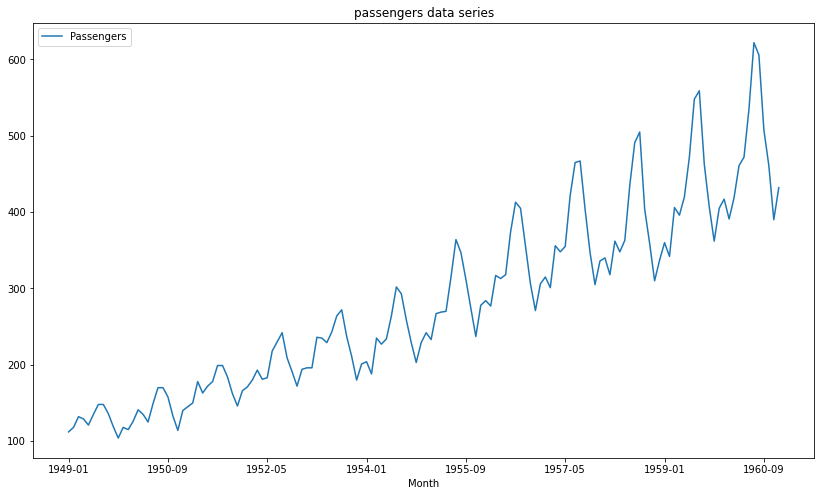
Here we can see that the data we are using is non-stationary because the number of passengers is integrated positively with time.

Now that we have all the things we require, we can perform our test on the time series.

Taking out the passengers number as a series.

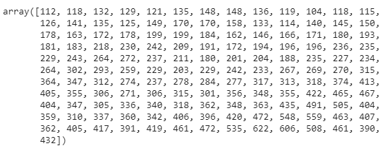
Performing the ADF test on the series:

Extracting the values from the results:

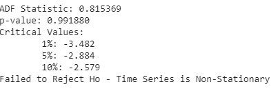
Here in the results, we can see that the p-value for time series is greater than 0.05, and we can say we fail to reject the null hypothesis and the time series is non-stationary.

Now, let’s check the test for stationary data.

Loading the data.

Checking for some head values of the data:

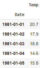
Here we can see that the data has the average temperature values for every day.

data.plot(figsize=(14,8), title='temperature data series')

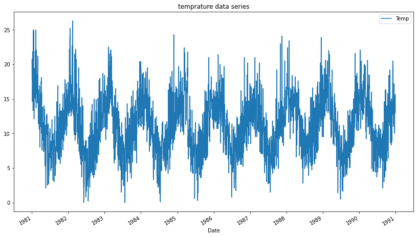
Here we can see that in the data, the larger value follows the next smaller value throughout the time series, so we can say the time series is stationary and check it with the ADF test.

Extracting temperature in a series.

Performing ADF test.

result = adfuller(series, autolag='AIC')

Checking the results:

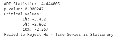
In the results, we can see that the p-value obtained from the test is less than 0.05 so we are going to reject the null hypothesis “Time series is stationary”, that means the time series is non-stationary.

In the article, we have seen why we need to perform the ADF test and the algorithms that the ADF and dickey-fuller test follow to make inferences about any time series. Statsmodel is one of the packages which allows us to perform many kinds of tests and analysis regarding time series analysis.

Best Face Swap AI Tools in 2024 – Remaker.ai Alternatives

Top 10 Cartoonist to Follow in 2024

The Best AI Search Engines in 2024 – Perplexity AI Alternatives

Different Types of Classification Algorithms

Top Most Important Reasons to Use Linux Operating System

Representation Learning – Complete Guide for Beginner

Bidirectional LSTM (Long-Short Term Memory) with Python Codes

Scribble Diffusion – Converts Doddles and Sketch to AI Images

Best AI Image Generator in 2024

What is Unstable Diffusion – Difference Between Stable Vs Unstable?

Difference Between NVIDIA H100 Vs A100: Which is the best GPU?

Top 10 Sentiment Analysis Dataset

Top 10 Space Observatories in India

How to Build Your First Generative AI Agent with Mistral 7B LLM

Join the forefront of data innovation at the Data Engineering Summit 2024, where industry leaders redefine technology’s future.

Subscribe to our Youtube channel and see how AI ecosystem works.

IMAGES

Null Hypothesis Significance Testing Overview
15 Null Hypothesis Examples (2024)
Hypothesis Testing- Meaning, Types & Steps
Null Hypothesis
Null hypothesis
t test null hypothesis example

VIDEO

Null & Alternative Hypothesis |Statistical Hypothesis #hypothesis #samplingdistribution #statistics
Hypothesis testing for meu when σ is known Hindi/Urdu lExample
Testing of Hypothesis
Writing the Null and Alternate Hypothesis in Statistics
Statistical Significance & Hypothesis Testing
Step-by-Step Guide to Hypothesis Testing: A Detailed Example of the 9 Essential Steps

COMMENTS

Null Hypothesis: Definition, Rejecting & Examples
The null hypothesis in statistics states that there is no difference between groups or no relationship between variables. It is one of two mutually exclusive hypotheses about a population in a hypothesis test. When your sample contains sufficient evidence, you can reject the null and conclude that the effect is statistically significant.
Null & Alternative Hypotheses
Revised on June 22, 2023. The null and alternative hypotheses are two competing claims that researchers weigh evidence for and against using a statistical test: Null hypothesis (H0): There's no effect in the population. Alternative hypothesis (Ha or H1): There's an effect in the population. The effect is usually the effect of the ...
Null hypothesis
Basic definitions. The null hypothesis and the alternative hypothesis are types of conjectures used in statistical tests to make statistical inferences, which are formal methods of reaching conclusions and separating scientific claims from statistical noise.. The statement being tested in a test of statistical significance is called the null hypothesis. . The test of significance is designed ...
9.1 Null and Alternative Hypotheses
The actual test begins by considering two hypotheses.They are called the null hypothesis and the alternative hypothesis.These hypotheses contain opposing viewpoints. H 0, the —null hypothesis: a statement of no difference between sample means or proportions or no difference between a sample mean or proportion and a population mean or proportion. In other words, the difference equals 0.
Hypothesis Testing
Table of contents. Step 1: State your null and alternate hypothesis. Step 2: Collect data. Step 3: Perform a statistical test. Step 4: Decide whether to reject or fail to reject your null hypothesis. Step 5: Present your findings. Other interesting articles. Frequently asked questions about hypothesis testing.
9.1: Null and Alternative Hypotheses
Review. In a hypothesis test, sample data is evaluated in order to arrive at a decision about some type of claim.If certain conditions about the sample are satisfied, then the claim can be evaluated for a population. In a hypothesis test, we: Evaluate the null hypothesis, typically denoted with \(H_{0}\).The null is not rejected unless the hypothesis test shows otherwise.
Statistical hypothesis test
A statistical hypothesis test is a method of statistical inference used to decide whether the data sufficiently support a particular hypothesis. ... An example of Neyman-Pearson hypothesis testing (or null hypothesis statistical significance testing) can be made by a change to the radioactive suitcase example. ...
What Is The Null Hypothesis & When To Reject It
Calculating the p-value is a critical part of null-hypothesis significance testing because it quantifies how strongly the sample data contradicts the null hypothesis. The level of statistical significance is often expressed as a p -value between 0 and 1. The smaller the p-value, the stronger the evidence that you should reject the null hypothesis.
Null Hypothesis Definition and Examples, How to State
Step 1: Figure out the hypothesis from the problem. The hypothesis is usually hidden in a word problem, and is sometimes a statement of what you expect to happen in the experiment. The hypothesis in the above question is "I expect the average recovery period to be greater than 8.2 weeks.". Step 2: Convert the hypothesis to math.
Null and Alternative Hypotheses
The actual test begins by considering two hypotheses.They are called the null hypothesis and the alternative hypothesis.These hypotheses contain opposing viewpoints. H 0: The null hypothesis: It is a statement about the population that either is believed to be true or is used to put forth an argument unless it can be shown to be incorrect beyond a reasonable doubt.
Statistical Hypothesis Testing Overview
Hypothesis testing is a crucial procedure to perform when you want to make inferences about a population using a random sample. These inferences include estimating population properties such as the mean, differences between means, proportions, and the relationships between variables. This post provides an overview of statistical hypothesis testing.
Understanding Null Hypothesis Testing
Null hypothesis testing is a formal approach to deciding whether a statistical relationship in a sample reflects a real relationship in the population or is just due to chance. The logic of null hypothesis testing involves assuming that the null hypothesis is true, finding how likely the sample result would be if this assumption were correct ...
An Introduction to Statistics: Understanding Hypothesis Testing and
HYPOTHESIS TESTING. A clinical trial begins with an assumption or belief, and then proceeds to either prove or disprove this assumption. In statistical terms, this belief or assumption is known as a hypothesis. Counterintuitively, what the researcher believes in (or is trying to prove) is called the "alternate" hypothesis, and the opposite ...
Null and Alternative Hypotheses
Some of the following statements refer to the null hypothesis, some to the alternate hypothesis. State the null hypothesis, H 0, and the alternative hypothesis. H a, in terms of the appropriate parameter (μ or p). The mean number of years Americans work before retiring is 34. At most 60% of Americans vote in presidential elections.
Examples of null and alternative hypotheses
It is the opposite of your research hypothesis. The alternative hypothesis--that is, the research hypothesis--is the idea, phenomenon, observation that you want to prove. If you suspect that girls take longer to get ready for school than boys, then: Alternative: girls time > boys time. Null: girls time <= boys time.
Choosing the Right Statistical Test
The test statistic tells you how different two or more groups are from the overall population mean, or how different a linear slope is from the slope predicted by a null hypothesis. Different test statistics are used in different statistical tests.
How to Write a Null Hypothesis (5 Examples)
Whenever we perform a hypothesis test, we always write a null hypothesis and an alternative hypothesis, which take the following forms: H0 (Null Hypothesis): Population parameter =, ≤, ≥ some value. HA (Alternative Hypothesis): Population parameter <, >, ≠ some value. Note that the null hypothesis always contains the equal sign.
Null Hypothesis
In other words, the null hypothesis is a hypothesis in which the sample observations results from the chance. It is said to be a statement in which the surveyors wants to examine the data. It is denoted by H 0. Null Hypothesis Symbol. In statistics, the null hypothesis is usually denoted by letter H with subscript '0' (zero), such that H 0 ...
Null hypothesis significance testing: a short tutorial
Abstract: "null hypothesis significance testing is the statistical method of choice in biological, biomedical and social sciences to investigate if an effect is likely". No, NHST is the method to test the hypothesis of no effect. I agree - yet people use it to investigate (not test) if an effect is likely.
Null Hypothesis
Null Hypothesis, often denoted as H0, is a foundational concept in statistical hypothesis testing. It represents an assumption that no significant difference, effect, or relationship exists between variables within a population. It serves as a baseline assumption, positing no observed change or effect occurring.
What does "Null Hypothesis Statistical Test" mean?
Learn the meaning of Null Hypothesis Statistical Test (a.k.a. NHST) in the context of A/B testing, a.k.a. online controlled experiments and conversion rate optimization. Detailed definition of Null Hypothesis Statistical Test, related reading, examples. Glossary of split testing terms.
Test statistics
The test statistic is a number calculated from a statistical test of a hypothesis. It shows how closely your observed data match the distribution expected under the null hypothesis of that statistical test. The test statistic is used to calculate the p value of your results, helping to decide whether to reject your null hypothesis.
5 Tips for Interpreting P-Values Correctly in Hypothesis Testing
Here are five essential tips for ensuring the p-value from a hypothesis test is understood correctly. 1. Know What the P-value Represents. First, it is essential to understand what a p-value is. In hypothesis testing, the p-value is defined as the probability of observing your data, or data more extreme, if the null hypothesis is true.
Augmented Dickey-Fuller (ADF) Test In Time-Series Analysis
The article will see the mathematics behind the test and how we can implement it in a time series. ADF (Augmented Dickey-Fuller) test is a statistical significance test which means the test will give results in hypothesis tests with null and alternative hypotheses. As a result, we will have a p-value from which we will need to make inferences ...
An Introduction to t Tests
The null hypothesis (H 0) is that the true difference between these group means is zero. The alternate hypothesis (H a) ... Test statistics | Definition, Interpretation, and Examples The test statistic is a number, calculated from a statistical test, used to find if your data could have occurred under the null hypothesis. ...