programming assignment 3 hash tables

Learn Python practically and Get Certified .

Popular Tutorials

Popular examples, reference materials, learn python interactively, dsa introduction.

• What is an algorithm?
• Data Structure and Types
• Why learn DSA?
• Asymptotic Notations
• Master Theorem
• Divide and Conquer Algorithm

Data Structures (I)

• Types of Queue
• Circular Queue
• Priority Queue

Data Structures (II)

• Linked List
• Linked List Operations
• Types of Linked List
• Heap Data Structure
• Fibonacci Heap
• Decrease Key and Delete Node Operations on a Fibonacci Heap

Tree based DSA (I)

• Tree Data Structure
• Tree Traversal
• Binary Tree
• Full Binary Tree
• Perfect Binary Tree
• Complete Binary Tree
• Balanced Binary Tree
• Binary Search Tree

Tree based DSA (II)

• Insertion in a B-tree
• Deletion from a B-tree
• Insertion on a B+ Tree
• Deletion from a B+ Tree
• Red-Black Tree
• Red-Black Tree Insertion
• Red-Black Tree Deletion

Graph based DSA

• Graph Data Structure
• Spanning Tree
• Strongly Connected Components
• Adjacency Matrix
• Adjacency List
• DFS Algorithm
• Breadth-first Search
• Bellman Ford's Algorithm

Sorting and Searching Algorithms

• Bubble Sort
• Selection Sort
• Insertion Sort
• Counting Sort
• Bucket Sort
• Linear Search
• Binary Search

Greedy Algorithms

• Greedy Algorithm
• Ford-Fulkerson Algorithm
• Dijkstra's Algorithm
• Kruskal's Algorithm
• Prim's Algorithm
• Huffman Coding
• Dynamic Programming
• Floyd-Warshall Algorithm
• Longest Common Sequence

Other Algorithms

• Backtracking Algorithm

Rabin-Karp Algorithm

DSA Tutorials

Linked list Data Structure

Bucket Sort Algorithm

• Linked List Operations: Traverse, Insert and Delete

The Hash table data structure stores elements in key-value pairs where

• Key - unique integer that is used for indexing the values
• Value - data that are associated with keys.

Hashing (Hash Function)

In a hash table, a new index is processed using the keys. And, the element corresponding to that key is stored in the index. This process is called hashing .

Let k be a key and h(x) be a hash function.

Here, h(k) will give us a new index to store the element linked with k .

To learn more, visit Hashing .

• Hash Collision

When the hash function generates the same index for multiple keys, there will be a conflict (what value to be stored in that index). This is called a  hash collision.

We can resolve the hash collision using one of the following techniques.

• Collision resolution by chaining
• Open Addressing: Linear/Quadratic Probing and Double Hashing

1. Collision resolution by chaining

In chaining, if a hash function produces the same index for multiple elements, these elements are stored in the same index by using a doubly-linked list.

If j is the slot for multiple elements, it contains a pointer to the head of the list of elements. If no element is present, j contains NIL .

Pseudocode for operations

2. Open Addressing

Unlike chaining, open addressing doesn't store multiple elements into the same slot. Here, each slot is either filled with a single key or left NIL .

Different techniques used in open addressing are:

i. Linear Probing

In linear probing, collision is resolved by checking the next slot.

h(k, i) = (h′(k) + i) mod m

• i = {0, 1, ….}
• h'(k) is a new hash function

If a collision occurs at h(k, 0) , then h(k, 1) is checked. In this way, the value of i is incremented linearly.

The problem with linear probing is that a cluster of adjacent slots is filled. When inserting a new element, the entire cluster must be traversed. This adds to the time required to perform operations on the hash table.

ii. Quadratic Probing

It works similar to linear probing but the spacing between the slots is increased (greater than one) by using the following relation.

h(k, i) = (h′(k) + c 1 i + c 2 i 2 ) mod m

• c 1 and c 2 are positive auxiliary constants,

iii. Double hashing

If a collision occurs after applying a hash function h(k) , then another hash function is calculated for finding the next slot.

h(k, i) = (h 1 (k) + ih 2 (k)) mod m

Good Hash Functions

A good hash function may not prevent the collisions completely however it can reduce the number of collisions.

Here, we will look into different methods to find a good hash function

1. Division Method

If k is a key and m is the size of the hash table, the hash function h() is calculated as:

h(k) = k mod m

For example, If the size of a hash table is 10 and k = 112 then h(k) = 112 mod 10 = 2 . The value of m must not be the powers of 2 . This is because the powers of 2 in binary format are 10, 100, 1000, … . When we find k mod m , we will always get the lower order p-bits.

2. Multiplication Method

h(k) = ⌊m(kA mod 1)⌋

• kA mod 1 gives the fractional part kA ,
• ⌊ ⌋ gives the floor value
• A is any constant. The value of A lies between 0 and 1. But, an optimal choice will be ≈ (√5-1)/2 suggested by Knuth.

3. Universal Hashing

In Universal hashing, the hash function is chosen at random independent of keys.

Python, Java and C/C++ Examples

Applications of hash table.

Hash tables are implemented where

• constant time lookup and insertion is required
• cryptographic applications
• indexing data is required

Table of Contents

• Open Addressing
• Good Hash Function
• Hash Table Implementation
• Applications

Sorry about that.

Related Tutorials

DS & Algorithms

Want to create or adapt books like this? Learn more about how Pressbooks supports open publishing practices.

7 Hashing and Hash Tables

Learning Objectives

After reading this chapter you will…

• understand what hash functions are and what they do.
• be able to use hash functions to implement an efficient search data structure, a hash table.
• understand the open addressing strategy for implementing hash tables.
• understand the potential problems with using hash functions for searching.
• be able to implement a hash table using data structure composition and the separate chaining strategy.

Introduction

In chapter 4, we explored a very important class of problems: searching. As the number of items increases, Linear Search becomes very costly, as every search costs O(n). Additionally, the real-world time cost of searching increases when the number of searches (also called queries) increases. For this reason, we explored sorting our “keys” (our unique identifiers) and then using Binary Search on data sets that get searched a lot. Binary Search improves our performance to O(log n) for searches. In this chapter, we explore ways to further improve search to approximately O(1) or constant time on average. There are some considerations, but with a good design, searches can be made extremely efficient. The key to this seemingly magic algorithm is the hash function. Let’s explore hashes a bit more in-depth.

Hash Functions

If you have ever eaten breakfast at a diner in the USA, you were probably served some hash browns. These are potatoes that have been very finely chopped up and cooked. In fact, this is where the “hash” of the hash function gets its name. A hash function takes a number, the key, and generates a new number using information in the original key value. So at some level, it takes information stored in the key, chops the bits or digits into parts, then rearranges or combines them to generate a new number. The important part, though, is that the hash function will always generate the same output number given the input key. There are many different types of hash functions. Let’s look at a simple one that hashes the key 137. We will use a small subscript of 2 when indicating binary numbers.

We can generate hashes using strings or text as well. We can extract letters from the string, convert them to numbers, and add them together. Here is an example of a different hash function that processes a string:

There are many hash functions that can be constructed for keys. For our purposes, we want hash functions that exhibit some special properties. In this chapter, we will be constructing a lookup table using hashes. Suppose we wanted to store student data for 100 students. If our hash function could take the student’s name as the key and generate a unique index for every student, we could store all their data in an array of objects and search using the hash. This would give us constant time, or O(1), lookups for any search! Students could have any name, which would be a vast set of possible keys. The hash function would look at the name and generate a valid array index in the range of 0 to 99.

The hash functions useful in this chapter map keys from a very large domain into a small range represented by the size of the table or array we want to use. Generally, this cannot be done perfectly, and we get some “ collisions ” where different keys are hashed to the same index. This is one of the main problems we will try to fix in this chapter. So one property of the hash function we want is that it leads to few collisions. Since a perfect hash is difficult to achieve, we may settle for an unbiased one. A hash function is said to be uniform if it hashes keys to indexes with roughly equal probability. This means that if the keys are uniformly distributed, the generated hash values from the keys should also be roughly uniformly distributed. To state that another way, when considered over all k keys, the probability h(k) = a is approximately the same as the probability that h(k) = b. Even with a nice hash function, collisions can still happen. Let’s explore how to tackle these problems.

Hash Tables

Once you have finished reading this chapter, you will understand the idea behind hash tables. A hash table is essentially a lookup table that allows extremely fast search operations. This data structure is also known as a hash map, associative array, or dictionary. Or more accurately, a hash table may be used to implement associative arrays and dictionaries. There may be some dispute on these exact terms, but the general idea is this: we want a data structure that associates a key and some value, and it must efficiently find the value when given the key. It may be helpful to think of a hash table as a generalization of an array where any data type can be used as an index. This is made possible by applying a hash function to the key value.

For this chapter, we will keep things simple and only use integer keys. Nearly all modern programming languages provide a built-in hash function or several hash functions. These language library–provided functions can hash nearly all data types. It is recommended that you use the language-provided hash functions in most cases. These are functions that generally have the nice properties we are looking for, and they usually support all data types as inputs (rather than just integers).

A Hash Table Using Open Addressing

Suppose we want to construct a fast-access database for a list of students. We will use the Student class from chapter 4. We will slightly alter the names though. For this example, we will use the variable name key rather than member_id to simplify the code and make the meaning a bit clearer.

We want our database data structure to be able to support searches using a search operation. Sometimes the term “find” is used rather than “search” for this operation. We will be consistent with chapter 4 and use the term “search” for this operation. As the database will be searched frequently, we want search to be very efficient. We also need some way to add and remove students from the database. This means our data structure should support the add and remove operations.

The first strategy we will explore with hash tables is known as open addressing . This means that we will allot some storage space in memory and place new data records into an open position addressed by the hash function. This is usually done using an array. Let the variable size represent the number of positions in the array. With the size of our array known, we can introduce a simple hash function where mod is the modulo or remainder operator.

This hash function maps the key to a valid array index. This can be done in constant time, O(1). When searching for a student in our database, we could do something like this:

This would ensure a constant-time search operation. There is a problem, though. Suppose our array had a size of 10. What would happen if we searched for the student with key 18 and another student with key 28? Well, 18 mod 10 is 8, and 28 mod 10 is 8. This simple approach tries to look for the same student in the same array address. This is known as a collision or a hash collision .

We have two options to deal with this problem. First, we could use a different hash function. There may be another way to hash the key to avoid these collisions. Some algorithms can calculate such a function, but they require knowledge of all the keys that will be used. So this is a difficult option most of the time. The second alternative would be to introduce some policy for dealing with these collisions. In this chapter, we will take the second approach and introduce a strategy known as probing . Probing tries to find the correct key by “probing” or checking other positions relative to the initial hashed address that resulted in the collision. Let’s explore this idea with a more detailed example and implementation.

Open Addressing with Linear Probing

Let us begin by specifying our hash table data structure. This class will need a few class functions that we will specify below, but first let’s give our hash table some data. Our table will need an array of Student records and a size variable.

To add new students to our data structure, we will use an add function. There is a simple implementation for this function without probing. We will consider this approach and then improve on it. Assume that the add function belongs to the HashTable class, meaning that table and size are both accessible without passing them to the function.

Once a student is added, the HashTable could find the student using the search function. We will have our search function return the index of the student in the array or −1 if the student cannot be found.

This approach could work assuming our hash was perfect. This is usually not the case though. We will extend the class to handle collisions. First, let’s explore an example of our probing strategy.

Suppose we try to insert a student, marked as “A,” into the database and find that the student’s hashed position is already occupied. In this example, student A is hashed to position 2, but we have a collision.

With probing, we would try the next position in the probe sequence . The probe sequence specifies which positions to try next. We will use a simple probe sequence known as linear probing . Linear probing will have us just try the next position in the array.

This figure shows that first we get a collision when trying to insert student A. Second, we probe the next position in the array and find that it is empty, so student A is inserted into this array slot. If another collision happens on the same hash position, linear probing has us continue to explore further into the array and away from the original hash position.

This figure shows that another collision will require more probing. You may now be thinking, “This could lead to trouble.” You would be right. Using open addressing with probing means that collisions can start to cause a lot of problems. The frequency of collisions will quickly lead to poor performance. We will revisit this soon when we discuss time complexity. For now, we have a few other problems with this approach.

Add and Search with Probing

Let us tackle a relatively simple problem first. How can we implement our probe sequence? We want our hash function to return the proper hash the first time it is used. If we have a collision, our hash needs to return the original value plus 1. If we have two collisions, we need the original value plus 2, and so on. For this, we will create a new hashing function that takes two input parameters.

With this function, hash(2,2) would give the value 4 as in the previous figure. In that example, when trying to insert student B, we get an initial collision followed by a second collision with student A that was just inserted. Finally, student B is inserted into position 4.

Did you notice the other problem? How will we check to see if the space in the array is occupied? There are a variety of approaches to solving this problem. We will take a simple approach that uses a secondary array of status values. This array will be used to mark which table spaces are occupied and which are available. We will add an integer array called status to our data structure. This approach will simplify the code and prepare our HashTable to support remove (delete) operations. The new HashTable will be defined as follows:

We will assign a status value of 0 to an empty slot and a value of 1 to an occupied slot. Now to check if a space is open and available, the code could just check to see if the status value at that index is 0. If the status is 1, the position is filled, and adding to that location results in a collision. Now let’s use this information to correct our add function for using linear probing. We will assume that all the status values are initialized with 0 when the HashTable is constructed.

Now that we can add students to the table, let us develop the search function to deal with collisions. The search function will be like add. For this algorithm, status[index] should be 1 inside the while-loop, but we will allow for −1 values a bit later. This is why 0 is not used here.

We need to discuss the last operation now: remove. The remove operation may also be called delete in some contexts. The meaning is the same though. We want a way to remove students from the database. Let’s think about what happens when a student is removed from the database. Think back to the collision example where student B is inserted into the database. What would happen if A was removed and then we searched for B?

If we just marked a position as open after a remove operation, we would get an error like the one illustrated above. With this sequence of steps, it seems like B is not in the table because we found an open position as we searched for it. We need to deal with this problem. Luckily, we have laid the foundation for a simple solution. Rather than marking a deleted slot as open, we will give it a deleted status code. In our status array, any value of −1 will indicate that a student was deleted from the table. This will solve the problem above by allowing searches to proceed past these deleted positions in the probe sequence.

The following function can be used to implement the remove function. This approach relies on our search function that returns the correct index. Notice how the status array is updated.

Depending on your implementation, you may also want to free the memory at table[index] at line 5. We are assuming that student records are stored directly in the array and will be overwritten on the next add operation for that position. If references are used, freeing the data may need to be explicit.

Take a careful look back at the search function to convince yourself that this is correct. When the status is −1, the search function should proceed through past collisions to work correctly. We now have a correct implementation of a hash table. There are some serious drawbacks though. Let us now discuss performance concerns with our hash table.

Complexity and Performance

We saw that adding more students to the hash table can lead to collisions. When we have collisions, the probing sequence places the colliding student near the original student record. Think about the situation below that builds off one of our previous examples:

Suppose that we try to add student C to the table and C’s key hashes to the index 3. No other student’s key hashes to position 3, but we still get 2 collisions. This clump of records is known as a cluster . You can see that a few collisions lead to more collisions and the clusters start to grow and grow. In this example, collisions now result if we get keys that hash to any index between 2 and 5.

What does this mean? Well, if the table is mostly empty and our hash function does a decent job of avoiding collisions, then add and search should both be very efficient. We may have a few collisions, but our probe sequences would be short and on the order of a constant number of operations. As the table fills up, we get some collisions and some clusters. Then with clustering, we get more collisions and more clustering as a result. Now our searches are taking many more operations, and they may approach O(n) especially when the table is full and our search key is not actually in the database. We will explore this in a bit more detail.

A load factor is introduced to quantify how full or empty the table is. This is usually denoted as α or the Greek lowercase alpha . We will just use an uppercase L. The load factor can be defined as simply the ratio of added elements to the total capacity. In our table, the capacity is represented by the size variable. Let n be the number of elements to be added to the database. Then the overall load factor for the hash table would be L = n / size. For our table, L must be less than 1, as we can only store as many students as we have space in the array.

How does this relate to runtime complexity? Well, in the strict sense, the worst-case performance for searches would be O(n). This is represented by the fact that when the table is full, we must check nearly all positions in the table. On the other hand, our analysis of Quick Sort showed that the expected worst-case performance can mean we get a very efficient and highly useful algorithm even if some cases may be problematic. This is the case with hash tables. Our main interest is in the average case performance and understanding how to avoid the worst-case situation. This is where the load factor comes into play. Donald Knuth is credited with calculating the average number of probes needed for linear probing in both a successful search and the more expensive unsuccessful search . Here, a successful search means that the item is found in the table. An unsuccessful search means the item was searched for but not found to be in the table. These search cost values depend on the L value. This makes sense, as a mostly empty table will be easy to insert into and yield few collisions.

The expected number of probes for a successful search with linear probing is as follows:

For unsuccessful searches , the number of probes is larger:

Let’s put these values in context. Suppose our table size is 50 and there are 10 student records inserted into the table giving a load factor of 10/50 = 0.2. This means on average a successful search needs 1.125 probes. If the table instead contains 45 students, we can expect an average of 5.5 probes with an L of 45/50 = 0.9. This is the average. Some may take longer. The unsuccessful search yields even worse results. With an L of 10/50 = 0.2, an unsuccessful search would yield an average of 1.28 probes. With a table of lead L = 45/50 = 0.9, the average number of probes would be 50.5. This is close to the worst-case O(n) performance.

We can see that the average complexity is heavily influenced by the load factor L. This is true of all open addressing hash table methods. For this reason, many hash table data structures will detect that the load is high and then dynamically reallocate a larger array for the data. This increases capacity and reduces the load factor. This approach is also helpful when the table accumulates a lot of deleted entries. We will revisit this idea later in the chapter. Although linear probing has some poor performance at high loads, the nature of checking local positions has some advantages with processor caches. This is another important idea that makes linear probing very efficient in practice.

The space complexity of a hash table should be clear. We need enough space to store the elements; therefore, the space complexity is O(n). This is true of all the open addressing methods.

Other Probing Strategies

One major problem with linear probing is that as collisions occur, clusters begin to grow and grow. This blocks other hash positions and leads to more collisions and therefore more clustering. One strategy to reduce the cluster growth is to use a different probing sequence. In this section, we will look at two popular alternatives to linear probing. These are the methods of quadratic probing and double hashing . Thanks to the design of our HashTable in the previous section, we can simply define new hash functions. This modular design means that changing the functionality of the data structure can be done by changing a single function. This kind of design is sometimes difficult to achieve, but it can greatly reduce repeated code.

Quadratic Probing

One alternative to linear probing is quadratic probing. This approach generates a probe sequence that increases by the square of the number of collisions. One simple form of quadratic probing could be implemented as follows:

The following illustration shows how this might improve on the problem of clustering we saw in the section on linear probing:

With one collision, student A still maps to position 3 because 2 + 1 2 = 3. When B is mapped though, it results in 2 collisions. Ultimately, it lands in position 6 because 2 + 2 2 = 6, as the following figure shows:

Figure 7.10

When student C is added, it will land in position 4, as 3 + 1 2 = 4. The following figure shows this situation:

Figure 7.11

Now instead of one large primary cluster, we have two somewhat smaller clusters. While quadratic probing reduces the problems associated with primary clustering, it leads to secondary clustering .

One other problem with quadratic probing comes from the probe sequence. Using the approach we showed where the hash is calculated using a formula like h(k) + c 2 , we will only use about size/2 possible indexes. Look at the following sequence: 1, 4, 9, 16, 25, 36, 49, 64, 81, 100, 121, 144. Now think about taking these values after applying mod 10. We get 1, 4, 9, 6, 5, 6, 9, 4, 1, 0, 1, 4. These give only 6 unique values. The same behavior is seen for any mod value or table size. For this reason, quadratic probing usually terminates once the number of collisions is half of the table size. We can make this modification to our algorithm by modifying the probing loop in the add and search functions.

For the add function, we would use

For the search function, we would use

When adding, it is assumed that encountering size/2 collisions means that the table is full. It is possible that this is incorrect. There may be open positions available even after quadratic probing has failed. If attempting to add fails, it is a good indicator that the load factor has become too high anyway, and the table needs to be expanded and rebuilt.

Double Hashing

In this section, we will look at an implementation of a hashing collision strategy that approaches the ideal strategy for an open addressed hash table. We will also discuss how to choose a good table size such that our hash functions perform better when our keys do not follow a random uniform distribution.

Choosing a Table Size

So far, we have chosen a table size of 10 in our examples. This has made it easy to think about what hash value is generated from a base-10 numerical key. This would be fine assuming our key distribution was truly uniform in the key domain. In practice, keys can have some properties that result in biases and ultimately nonuniform distributions. Take, for example, the use of a memory address as a key. On many computer systems, memory addresses are multiples of 4. As another example, in English, the letter “e” is far more common than other letters. This might result in keys generated from ASCII text having a nonuniform distribution.

Let’s look at an example of when this can become a problem. Suppose we have a table of size 12 and our keys are all multiples of 4. This would result in all keys being initially hashed to only the indexes 0, 4, or 8. For both linear probing and quadratic probing, any key with the initial hash value will give the same probing sequence. So this example gives an especially bad situation resulting in poor performance under both linear probing and quadratic probing. Now suppose that we used a prime number rather than 12, such as 13. The table below gives a sequence of multiples of 4 and the resulting mod values when divided by 12 and 13.

Figure 7.12

It is easy to see that using 13 performs much better than 12. In general, it is favored to use a table size that is a prime value. The approach of using a prime number in hash-based indexing is credited to Arnold Dumey in a 1956 work. This helps with nonuniform key distributions.

Implementing Double Hashing

As the name implies, double hashing uses two hash functions rather than one. Let’s look at the specific problem this addresses. Suppose we are using the good practice of having size be a prime number. This still cannot overcome the problem in probing methods of having the same initial hash index. Consider the following situation. Suppose k 1 is 13 and k 2 is 26. Both keys will generate a hashed value of 0 using mod 13. The probing sequence for k 1 in linear probing is this:

h(k 1 ,0) = 0, h(k 1 ,1) = 1, h(k 1 ,2) = 2, and so on. The same is true for k 2 .

Quadratic probing has the same problem:

h Q (k 1 , 0) = 0, h Q (k 1 , 1) = 1, h Q (k 1 , 2) = 2. This is the same probe sequence for k 2 .

Let’s walk through the quadratic probing sequence a little more carefully to make it clear. Recall that

h Q (k,c) = (k mod size + c 2 ) mod size

using quadratic probing. The following table gives the probe sequence for k 1 = 13 and k 2 = 26 using quadratic probing:

Figure 7.13

The probe sequence is identical given the same initial hash. To solve this problem, double hashing was introduced. The idea is simple. A second hash function is introduced, and the probe sequence is generated by multiplying the number of collisions by a second hash function. How should we choose this second hash function? Well, it turns out that choosing a second prime number smaller than size works well in practice.

Let’s create two hash functions h 1 (k) and h 2 (k). Now let p 1 be a prime number that is equal to size. Let p 2 be a prime number such that p 2 < p 1 . We can now define our functions and the final double hash function:

h 1 (k) = k mod p 1

h 2 (k) = k mod p 2 .

The final function to generate the probe sequence is here:

h(k, c) = (h 1 (k) + c*h 2 (k)) mod size.

Let’s let p 1 = 13 = size and p 2 = 11 for our example. How would this change the probe sequence for our keys 13 and 26? In this case h 1 (13) = h 1 (26) = 0, but h 2 (13) = 2, h 2 (26) = 4.

Consider the following table:

Figure 7.14

Now that we understand double hashing, let’s start to explore one implementation in code. We will create two hash functions as follows:

The second hash function will use a variable called prime , which has a value that is a prime number smaller than size.

Finally, our hash function with a collisions parameter is developed below:

As before, these can be easily added to our HashTable data structure without changing much of the code. We would simply add the hashOne and hashTwo functions and replace the two-parameter hash function.

Complexity of Open Addressing Methods

Open addressing strategies for implementing hash tables that use probing all have some features in common. Generally speaking, they all require O(n) space to store the data entries. In the worst case, search-time cost could be as bad as O(n), where the data structure checks every entry for the correct key. This is not the full story though.

As we discussed before with linear probing, when a table is mostly empty, adding data or searching will be fast. First, check the position in O(1) with the hash. Next, if the key is not found and the table is mostly empty, we will check a small constant number of probes. Search and insert would be O(1), but only if it’s mostly empty. The next question that comes to mind is “What does ‘mostly empty’ mean?” Well, we used a special value to quantify the “fullness” level of the table. We called this the load factor, which we represented with L.

Let’s explore L and how it is used to reason about the average runtime complexity of open addressing hash tables. To better understand this idea, we will use an ideal model of open addressing with probing methods. This is known as uniform hashing, which was discussed a bit before. Remember the problems of linear probing and quadratic probing. If any value gives the same initial hash, they end up with the same probe sequence. This leads to clustering and degrading performance. Double hashing is a close approximation to uniform hashing. Let’s consider double hashing with two distinct keys, k 1 and k 2. We saw that when h 1 (k 1 ) = h 1 (k 2 ), we can still get a different probe sequence if h 2 (k 1 ) ≠ h 2 (k 2 ). An ideal scenario would be that every unique key generates a unique but uniform random sequence of probe indexes. This is known as uniform hashing. Under this model, thinking about the average number of probes in a search is a little easier. Let’s think this through.

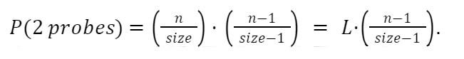
Remember that the load on the table is the ratio of filled to the total number of available positions in the table. If n elements have been inserted into the table, the load is L = n / size. Let’s consider the case of an unsuccessful search. How many probes would we expect to make given that the load is L? We will make at least one check, but next, the probability that we would probe again would be L. Why? Well, if we found one of the (size − n) open positions, the search would have ended without probing. So the probability of one unsuccessful probe is L. What about the probability of two unsuccessful probes? The search would have failed in the first probe with probability L, and then it would fail again in trying to find one of the (n − 1) occupied positions among the (size − 1) remaining available positions. This leads to a probability of

Things would progress from there. For 3 probes, we get the following:

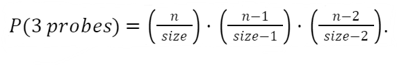
On and on it goes. We extrapolate out to x probes:

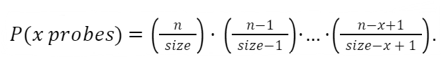
This sequence would be smaller than assuming a probability of L for every missed probe. We could express this relationship with the following equation:

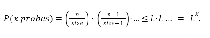
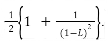
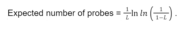
This gives us the probability of having multiple failed probes. We now want to think about the expected number of probes. One failed probe has the probability of L, and having more failed probes is less likely. To calculate the expected number of probes, we need to add the probabilities of all numbers of probes. So the P(1 probe) + P(2 probes)…on to infinity. You can think of this as a weighted average of all possible numbers of probes. A more likely number of probes contributes more to the weighted average. It turns out that we can calculate a value for this infinite series. The sum will converge to a specific value. We arrive at the following formula using the geometric series rule to give a bound for the number of probes in an unsuccessful search:

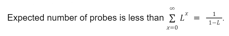
This equation bounds the expected number of probes or comparisons in an unsuccessful search. If 1/(1−L) is constant, then searches have an average case runtime complexity of O(1). We saw this in our analysis of linear probing where the performance was even worse than for the ideal uniform hashing.

For one final piece of analysis, look at the plot of 1/(1−L) between 0 and 1. This demonstrates just how critical the load factor can be in determining the expected complexity of hashing. This shows that as the load gets very high, the cost rapidly increases.

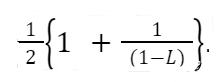
For completeness, we will present the much better performance of a successful search under uniform hashing:

Successful searches scale much better than unsuccessful ones, but they will still approach O(n) as the load gets high.

An alternative strategy to open addressing is known as chaining or separate chaining . This strategy uses separate linked lists to handle collisions. The nodes in the linked list are said to be “chained” together like links on a chain. Our records are then organized by keeping them on “separate chains.” This is the metaphor that gives the data structure its name. Rather than worrying about probing sequences, chaining will just keep a list of all records that collided at a hash index.

This approach is interesting because it represents an extremely powerful concept in data structures and algorithms, composition . Composition allows data structures to be combined in multiple powerful ways. How does it work? Well, data structures hold data, right? What if that “data” was another data structure? The specific composition used by separate chaining is an array of linked lists . To better understand this concept, we will visualize it and work through an example. The following image shows a chaining-based hash table after 3 add operations. No collisions have occurred yet:

Figure 7.16

The beauty of separate chaining is that both adding and removing records in the table are made extremely easy. The complexity of the add and remove operations is delegated to the linked list. Let’s assume the linked list supports add and remove by key operations on the list. The following functions give example implementations of add and remove for separate chaining. We will use the same Student class and the simple hash function that returns the key mod size.

The add function is below. Keep in mind that table[index] here is a linked list object:

Here is the remove function that, again, relies on the linked list implementation of remove:

When a Student record needs to be added to the table, whether a collision occurs or not, the Student is simply added to the linked list. See the diagram below:

When considering the implementation, collisions are not explicitly considered. The hash index is calculated, and student A is inserted by asking the link list to insert it. Let’s follow a few more add operations.

Suppose a student, B, is added with a hash index of 2.

Figure 7.18

Now if C is added with a hash index of 3, it would be placed in the empty list at position 3 in the array.

Figure 7.19

Here, the general idea of separate chaining is clear. Maybe it is also clear just how this could go wrong. In the case of search operations, finding the student with a given key would require searching for every student in the corresponding linked list. As you know from chapter 4, this is called Linear Search , and it requires O(n) operations, where n is the number of items in the list. For the separate chaining hash table, the length of any of those individual lists is hoped to be a small fraction of the total number of elements, n. If collisions are very common, then the size of an individual linked list in the data structure would get long and approach n in length. If this can be avoided and every list stays short, then searches on average take a constant number of operations leading to add, remove, and search operations that require O(1) operations on average. In the next section, we will expand on our implementation of a separate chaining hash table.

Separate Chaining Implementation

For our implementation of a separate chaining hash table, we will take an object-oriented approach. Let us assume that our data are the Student class defined before. Next, we will define a few classes that will help us create our hash table.

We will begin by defining our linked list. You may want to review chapter 4 before proceeding to better understand linked lists. We will first define our Node class and add a function to return the key associated with the student held at the node. The node class holds the connections in our list and acts as a container for the data we want to hold, the student data. In some languages, the next variable needs to be explicitly declared as a reference or pointer to the next Node.

We will now define the data associated with our LinkedList class. The functions are a little more complex and will be covered next.

Our list will just keep track of references to the head and tail Nodes in the list. To start thinking about using this list, let’s cover the add function for our LinkedList. We will add new students to the end of our list in constant time using the tail reference. We need to handle two cases for add. First, adding to an empty list means we need to set our head and tail variables correctly. All other cases will simply append to the tail and update the tail reference.

Searching in the list will use Linear Search . Using the currentNode reference, we check every node for the key we are looking for. This will give us either the correct node or a null reference (reaching the end of the list without finding it).

You may notice that we return currentNode regardless of whether the key matches or not. What we really want is either a Student object or nothing. We sidestepped this problem with open addressing by returning −1 when the search failed or the index of the student record when it was found. This means upstream code needs to check for the −1 before doing something with the result. In a similar way here, we send the problem upstream. Users of the code will need to check if the returned node reference is null. There are more elegant ways to solve this problem, but they are outside of the scope of the textbook. Visit the Wikipedia article on the Option Type for some background. For now, we will ask the user of the class to check the returned Node for the Student data.

To finish our LinkedList implementation for chaining, we will define our remove function. As remove makes modifications to our list structure, we will take special care to consider the different cases that change the head and tail members of the list. We will also use the convention of returning the removed node. This will allow the user of the code to optionally free its memory.

Now we will define our hash table with separate chaining. In the next code piece, we will define the data of our HashTable implemented with separate chaining. The HashTable’s main piece of data is the composed array of LinkedLists. Also, the simple hash function is defined (key mod size).

Here the simplicity of the implementation shines. The essential operations of the HashTable are delegated to LinkedList, and we get a robust data structure without a ton of programming effort! The functions for the add, search, and remove operations are presented below for our chaining-based HashTable:

One version of remove is provided below:

Some implementations of remove may expect a node reference to be given. If this is the case, remove could be implemented in constant time assuming the list is doubly linked. This would allow the node to be removed by immediately accessing the next and previous nodes. We have taken the approach of using a singly linked list and essentially duplicating the search functionality inside the LinkedList’s remove function.

Not bad for less than 30 lines of code! Of course, there is more code in each of the components. This highlights the benefit of composition. Composing data structures opens a new world of interesting and useful data structure combinations.

Separate Chaining Complexity

Like with open addressing methods, the worst-case performance of search (and our remove function) is O(n). Probing would eventually consider nearly all records in our HashTable. This makes the O(n) complexity clear. Thinking about the worst-case performance for chaining may be a little different. What would happen if all our records were hashed to the same list? Suppose we inserted n Students into our table and that they all shared the same hash index. This means all Students would be inserted into the same LinkedList. Now the complexity of these operations would all require examining nearly all student records. The complexity of these operations in the HashTable would match the complexity of the LinkedList, O(n).

Now we will consider the average or expected runtime complexity. With the assumption that our keys are hashed into indexes following a simple uniform distribution, the hash function should, on average, “evenly” distribute the records along all the lists in our array. Here “evenly” means approximately evenly and not deviating too far from an even split.

Let’s put this in more concrete terms. We will assume that the array for our table has size positions, and we are trying to insert n elements into the table. We will use the same load factor L to represent the load of our table, L = n / size. One difference from our open addressing methods is that now our L variable could be greater than 1. Using linked lists means that we can store more records in all of the lists than we have positions in our array of lists. When n Student records have been added to our chaining-based HashTable, they should be approximately evenly distributed between all the size lists in our array. This means that the n records are evenly split between size positions. On average, each list contains approximately L = n / size nodes. Searching those lists would require O(L) operations. The expected runtime cost for an unsuccessful search using chaining is often represented as O(1 + L). Several textbooks report the complexity this way to highlight the fact that when L is small (less than 1) the cost of computing the initial hash dominates the 1 part of the O(1 + L). If L is large, then it could dominate the complexity analysis. For example, using an array of size 1 would lead to L = n / 1 = n. So we get O(1 + L) = O(1 + n) = O(n). In practice, the value of L can be kept low at a small constant. This makes the average runtime of search O(1 + L) = O(1 + c) for some small constant c. This gives us our average runtime of O(1) for search, just as we wanted!

For the add operation, using the tail reference to insert records into the individual lists gives O(1) time cost. This means adding is efficient. Some textbooks report the complexity of remove or delete to be O(1) using a doubly linked list. If the Node’s reference is passed to the remove function using this implementation, this would give us an O(1) remove operation. This assumes one thing though. You need to get the Node from somewhere. Where might we get this Node? Well, chances are that we get it from a search operation. This would mean that to effectively remove a student by its key requires O(1 + L) + O(1) operations. This matches the performance of our implementation that we provided in the code above.

The space complexity for separate chaining should be easy to understand. For the number of records we need to store, we will need that much space. We would also need some extra memory for references or pointer variables stored in the nodes of the LinkedLists. These “linking” variables increase overall memory consumption. Depending on the implementation, each node may need 1 or 2 link pointers. This memory would only increase the memory cost by a constant factor. The space required to store the elements of a separate chaining HashTable is O(n).

Design Trade-Offs for Hash Tables

So what’s the catch? Hash tables are an amazing data structure that has attracted interest from computer scientists for decades. These hashing-based methods have given a lot of benefits to the field of computer science, from variable lookups in interpreters and compilers to fast implementations of sets, to name a few uses. With hash tables, we have smashed the already great search performance of Binary Search at O(log n) down to the excellent average case performance of O(1). Does it sound too good to be true? Well, as always, the answer is “It depends.” Learning to consider the performance trade-offs of different data structures and algorithms is an essential skill for professional programmers. Let’s consider what we are giving up in getting these performance gains.

The great performance scaling behavior of search is only in the average case. In practice, this represents most of the operations of the hash tables, but the possibility for extremely poor performance exists. While searching on average takes O(1), the worst-case time complexity is O(n) for all the methods we discussed. With open addressing methods, we try to avoid O(n) performance by being careful about our load factor L. This means that if L gets too large, we need to remove all our records and re-add them into a new larger array. This leads to another problem, wasted space. To keep our L at a nice value of, say, 0.75, that means that 25% of our array space goes unused. This may not be a big problem, but that depends on your application and system constraints. On your laptop, a few missing megabytes may go unnoticed. On a satellite or embedded device, lost memory may mean that your costs go through the roof. Chaining-based hash tables do not suffer from wasted memory, but as their load factor gets large, average search performance can suffer also. Again, a common practice is to remove and re-add the table records to a larger array once the load crosses a threshold. It should be noted again though that separate chaining already requires a substantial amount of extra memory to support linking references. In some ways, these memory concerns with hash tables are an example of the speed-memory trade-off , a classic concept in computer science. You will often find that in many cases you can trade time for space and space for time. In the case of hash tables, we sacrifice a little extra space to speed up our searches.

Another trade-off we are making may not be obvious. Hash tables guarantee only that searches will be efficient. If the order of the keys is important, we must look to another data structure. This means that finding the record with key 15 tells us nothing about the location of records with key 14 or 16. Let’s look at an example to better understand this trade-off in which querying a range might be a problem for hash tables compared to a Binary Search.

Suppose we gave every student a numerical identifier when they enrolled in school. The first student got the number 1, the second student got the number 2, and so on. We could get every student that enrolled in a specific time period by selecting a range. Suppose we used chaining to store our 2,000 students using the identifier as the key. Our 2,000 students would be stored in an array of lists, and the array’s size is 600. This means that on average each list contains between 3 and 4 nodes (3.3333…). Now we need to select 20 students that were enrolled at the same time. We need all the records for students whose keys are between 126 to 145 (inclusive). For a hash table, we would first search for key 126, add it to the list, then 127, then 128, and so on. Each search takes about three operations, so we get approximately 3.3333 * 20 = 66.6666 operations. What would this look like for a Binary Search? In Binary Search, the array of records is already sorted. This means that once we find the record with key 126, the record with key 127 is right next to it. The cost here would be log 2 (2000) + 20. This supposes that we use one Binary Search and 20 operations to add the records to our return list. This gives us approximately log 2 (2000) + 20 = 10.9657 + 20 = 30.9657. That is better than double our hash table implementation. However, we also see that individual searches using the hash table are over 3 times as fast as the Binary Search (10.6657 / 3.333 = 3.2897).

• Using linear probing with a table of size 13, make the following changes: add key 12; add key 13; add key 26; add key 6; add key 14, remove 26, add 39.
• Using quadratic probing with a table of size 13, make the following changes: add key 12; add key 13; add key 26; add key 6; add key 14, remove 26, add 39.
• Using double hashing with a table of size 13, make the following changes: add key 12; add key 13; add key 26; add key 6; add key 14, remove 26, add 39.
• Implement a hash table using linear probing as described in the chapter using your language of choice, but substitute the Student class for an integer type. Also, implement a utility function to print a representation of your table and the status associated with each open slot. Once your implementation is complete, execute the sequence of operations described in exercise 1, and print the table. Do your results match the paper results from exercise 1?
• Extend your linear probing hash table to have a load variable. Every time a record is added or removed, recalculate the load based on the size and the number of records. Add a procedure to create a new array that has size*2 as its new size, and add all the records to the new table. Recalculate the load variable when this procedure is called. Have your table call this rehash procedure anytime the load is greater than 0.75.
• Think about your design for linear probing. Modify your design such that a quadratic probing HashTable or a double hashing HashTable could be created by simply inheriting from the linear probing table and overriding one or two functions.
• Implement a separate chaining-based HashTable that stores integers as the key and the data. Compare the performance of the chaining-based hash table with linear probing. Generate 100 random keys in the range of 1 to 20,000, and add them to a linear probing-based HashTable with a size of 200. Add the same keys to a chaining-based HashTable with a size of 50. Once the tables are populated, time the execution of conducting 200 searches for randomly generated keys in the range. Which gave the better performance? Conduct this test several times. Do you see the same results? What factors contributed to these results?

Cormen, Thomas H., Charles E. Leiserson, Ronald L. Rivest, and Clifford Stein. Introduction to Algorithms , 2nd ed. Cambridge, MA: The MIT Press, 2001.

Dumey, Arnold I. “Indexing for Rapid Random Access Memory Systems,” Computers and Automation 5, no. 12 (1956): 6–9.

Flajolet, P., P. Poblete, and A. Viola. “On the Analysis of Linear Probing Hashing,” Algorithmica 22, no. 4 (1998): 490–515.

Knuth, Donald E. “Notes on ‘Open’ Addressing.” 1963. https://jeffe.cs.illinois.edu/teaching/datastructures/2011/notes/knuth-OALP.pdf.

Malik, D. S. Data Structures Using C++ . Cengage Learning, 2009.

An Open Guide to Data Structures and Algorithms by Paul W. Bible and Lucas Moser is licensed under a Creative Commons Attribution 4.0 International License , except where otherwise noted.

Share This Book

Princeton University COS 217:  Introduction to Programming Systems

Assignment 3:  a hash table adt.

A hash table is a collection of buckets . Each bucket is a collection of bindings .  Each binding consists of a key and a value .  A key uniquely identifies its binding; a value is data that is somehow pertinent to its key.  The mapping of bindings to buckets is determined by the hash table's hash function .  A hash function accepts a binding's key and bucket count, and returns the number of the bucket in which that binding should reside.

A collision occurs when more than one binding is mapped to the same bucket.  A good hash function distributes bindings fairly uniformly across the hash table's buckets, and thus minimizes collisions.  A bad hash function is one that generates many collisions.  With a good hash function, the retrieve/insert/delete performance of a hash table is very fast.

In principle, the user/client/customer of the Table ADT need not be concerned about its implementation; the user/client/customer is concerned only with the Table's interface.  However in practice the user/client/customer of the Table ADT must choose a Set implementation (either the one that uses arrays or the one that uses a tree) and a bucket count.  In Part 2 of the assignment your job is to analyze the efficiency of the Table ADT under various conditions, and thus provide guidance to the user/client/customer about which implementation and bucket count to choose.

Part 1:  The Table ADT

The table interface.

The Table_new function should return a new Table.  The parameter iBucketCount is the number of buckets that the Table will contain.  The parameter pfCompare is a pointer to a compare function that the Table will use to compare keys.  The function *pfCompare should return a negative integer if there is a "less than" relationship between the two given keys, a positive integer if there is a "greater than" relationship between the two given keys, and zero if the two given keys are equal.  The parameter pfHash is a pointer to a hash function that the Table will use to assign bindings to buckets.  It should be a checked runtime error for iBucketCount to be less than 1, for pfCompare to be NULL, or for pfHash to be NULL..

The TableIter Interface

The implementations.

Of course you should implement your Table ADT as a hash table.  Each bucket of a Table should be a Set, as specified in Assignment 2.  In that manner a Table should be composed of Sets.  You should use the given Set and SetIter ADTs (and not your own) .  

Part 2:  The Performance Analysis

Suppose you have sold your Table et al ADTs to customers.  Further suppose that your customers are requesting some guidance concerning efficient use of your ADTs.

Generic Analysis

Customer #1 has purchased your ADTs with the intention of using them in a variety of projects.  The customer asks you for general guidelines about which ADT to use when.  In particular, the customer asks for guidelines organized along four dimensions:

• Table implementation :  Table/Set/array, Table/Set/tree
• Function :  put, remove, get
• Bucket count :  1, 100
• Data size :  10 items, 100 items, 1000 items, 10000 items
• We recommend that you use the Set/array ADT when...
• We recommend that you use the Set/tree ADT when...
• We recommend that you use the Table/Set/array ADT when...
• We recommend that you use the Table/Set/tree ADT when...

Specific Analysis

Customer #2 has a more specific question.  The customer will be using your Table/Set/tree ADT in an application that is very similar to timetable, where the bucket count is 100 and the number of items is 10000 .  In the hope of improving efficiency, the customer is considering rewriting the hash and compare functions in assembly language.  The customer anticipates that the translation to assembly language will double the speed of those functions.  More precisely, the time spent executing those functions and their descendants will be cut in half.  The customer asks if the translation to assembly language is worth the effort. That is, how much will doubling the speed of the hash and compare functions impact the efficiency of the overall program?

Use the statistics produced by the gprof tool to formulate a one sentence response to Customer #2.  Be as specific as possible about the performance gain.  Place the response in your readme file.

• set.h contains an interface for the Set ADT.
• setarray.o and settree.o contain array and binary search tree (respectively) implementations of the Set ADT.  
• testtable.c contains a minimal test program that illustrates typical usage of the Table and TableIter ADTs.  You can use it as the basis for developing your own programs to test your Table and TableIter ADTs.
• timetable.c contains a program that you can use to further test your Table ADT, and to collect performance statistics.
• stats.h and stats.c define an ADT that is used by the timetable program.
• test10.txt , test100.txt , test1000.txt, and test10000.txt contain data that the timetable program can read.
• table.h should contain the interface for the Table and TableIter ADTs.
• table.c should contain the implementation of the Table and TableIter ADTs.
• readme should contain your name, and any information that will help us to grade your work in the most favorable light.  In particular you should describe all known bugs in your readme file.  It should also contain the performance analyses described above.

Programming Assignment #3

CS163: Data Structures

Problem Statement:

Hash tables are very useful in situations where an individual wants to quickly find their data by the “value” or “search key”.   You could think of them as similar to an array, except the client program uses a “key” instead of an “index” to get to the data. The key is then mapped through the hash function which turns it into an index!

You have decided to write a table abstract data type, using a hash table/function with chaining (for collision resolution), to support searching for interesting web sites. Your search key is the topic that someone is interested in and the list of appropriate web sites is displayed (just the link) that pertain to that particular subject matter. A web site may have many different subjects that it can be searched upon.

Abstract Data Type:

Write a C++ program that implements and uses a table abstract data type to store, search, and remove web site links and their subject lists.

What does retrieve need to do? It needs to supply back to the calling routine information about all of the web sites that contain the search key. Retrieve, since it is an ADT operation, should not correspond with the user (i.e., it should not prompt, echo, input, or output data).

Evaluate the performance of storing and retrieving items from this table. Monitor the number of collisions that occur for a given set of data that you select. Make sure your hash table is small enough that collisions actually do occur, even without vast quantities of data so that you can get an understanding of how chaining works. Try different table sizes, and evaluate the performance (i.e., the length of the chains!). Although, remember to make the hash table size a prime number.

Implement the abstract data type using a separate header file (.h) and implementation file (.cpp). Only include header files when absolutely necessary. Never include .cpp files!

Syntax Requirements:

1) Use iostream.h for all I/O; do not use stdio.h

2) Implement the table ADT as a class; provide a constructor and a destructor.

3) Make sure to protect the data members so that the main() program does not have direct access.

4) Your main() should allow the user to interactively insert, delete, or retrieve items from the table. ***THE MAIN PROGRAM SHOULD NOT BE AWARE THAT HASHING IS BEING DONE! ***

REMINDERS: Every program must have a comment at the beginning with your first and last name , the class (CS163) and section , the name of the file , and the assignment number . This is essential!

Instantly share code, notes, and snippets.

sirenko / Data Structures and Algorithms-Coursera.org

• Download ZIP
• Star ( 3 ) 3 You must be signed in to star a gist
• Fork ( 1 ) 1 You must be signed in to fork a gist
• Embed Embed this gist in your website.
• Share Copy sharable link for this gist.
• Clone via HTTPS Clone using the web URL.
• Learn more about clone URLs
• Save sirenko/795c2aa60484d148780e4629750cfa0b to your computer and use it in GitHub Desktop.

Data Structures and Algorithms | UC San Diego

Data structures and algorithms specialization, master algorithmic programming techniques. learn algorithms through programming and advance your software engineering or data science career.

About This Specialization

This specialization is a mix of theory and practice: you will learn algorithmic techniques for solving various computational problems and will implement about 100 algorithmic coding problems in a programming language of your choice. No other online course in Algorithms even comes close to offering you a wealth of programming challenges that you may face at your next job interview. To prepare you, we invested over 3000 hours into designing our challenges as an alternative to multiple choice questions that you usually find in MOOCs. Sorry, we do not believe in multiple choice questions when it comes to learning algorithms…or anything else in computer science! For each algorithm you develop and implement, we designed multiple tests to check its correctness and running time — you will have to debug your programs without even knowing what these tests are! It may sound difficult, but we believe it is the only way to truly understand how the algorithms work and to master the art of programming. The specialization contains two real-world projects: Big Networks and Genome Assembly . You will analyze both road networks and social networks and will learn how to compute the shortest route between New York and San Francisco (1000 times faster than the standard shortest path algorithms!) Afterwards, you will learn how to assemble genomes from millions of short fragments of DNA and how assembly algorithms fuel recent developments in personalized medicine.

COURSE 1 - Algorithmic Toolbox

Current session: Jan 15

The course covers basic algorithmic techniques and ideas for computational problems arising frequently in practical applications: sorting and searching, divide and conquer, greedy algorithms, dynamic programming. We will learn a lot of theory: how to sort data and how it helps for searching; how to break a large problem into pieces and solve them recursively; when it makes sense to proceed greedily; how dynamic programming is used in genomic studies. You will practice solving computational problems, designing new algorithms, and implementing solutions efficiently (so that they run in less than a second).

WEEK 1 - Programming Challenges

Welcome to the first module of Data Structures and Algorithms! Here we will provide an overview of where algorithms and data structures are used (hint: everywhere) and walk you through a few sample programming challenges. The programming challenges represent an important (and often the most difficult!) part of this specialization because the only way to fully understand an algorithm is to implement it. Writing correct and efficient programs is hard; please don’t be surprised if they don’t work as you planned—our first programs did not work either! We will help you on your journey through the specialization by showing how to implement your first programming challenges. We will also introduce testing techniques that will help increase your chances of passing assignments on your first attempt. In case your program does not work as intended, we will show how to fix it, even if you don’t yet know which test your implementation is failing on.

• Video · Welcome!
• Programming Assignment · Programming Assignment 1: Programming Challenges
• Practice Quiz · Solving Programming Challenges
• Reading · Optional Videos and Screencasts
• Video · Solving the Sum of Two Digits Programming Challenges (screencast)
• Video · Solving the Maximum Pairwise Product Programming Challenge: Improving the Naive Solution, Testing, Debugging
• Video · Stress Test - Implementation
• Video · Stress Test - Find the Test and Debug
• Video · Stress Test - More Testing, Submit and Pass!
• Reading · Acknowledgements

WEEK 2 - Algorithmic Warm-up

In this module you will learn that programs based on efficient algorithms can solve the same problem billions of times faster than programs based on naïve algorithms. You will learn how to estimate the running time and memory of an algorithm without even implementing it. Armed with this knowledge, you will be able to compare various algorithms, select the most efficient ones, and finally implement them as our programming challenges!

• Video · Why Study Algorithms?
• Video · Coming Up
• Video · Problem Overview
• Video · Naive Algorithm
• Video · Efficient Algorithm
• Reading · Resources
• Video · Problem Overview and Naive Algorithm
• Video · Computing Runtimes
• Video · Asymptotic Notation
• Video · Big-O Notation
• Video · Using Big-O
• Practice Quiz · Logarithms
• Practice Quiz · Big-O
• Practice Quiz · Growth rate
• Video · Course Overview
• Programming Assignment · Programming Assignment 2: Algorithmic Warm-up

WEEK 3 - Greedy Algorithms

In this module you will learn about seemingly naïve yet powerful class of algorithms called greedy algorithms. After you will learn the key idea behind the greedy algorithms, you may feel that they represent the algorithmic Swiss army knife that can be applied to solve nearly all programming challenges in this course. But be warned: with a few exceptions that we will cover, this intuitive idea rarely works in practice! For this reason, it is important to prove that a greedy algorithm always produces an optimal solution before using this algorithm. In the end of this module, we will test your intuition and taste for greedy algorithms by offering several programming challenges.

• Video · Largest Number
• Video · Car Fueling
• Video · Car Fueling - Implementation and Analysis
• Video · Main Ingredients of Greedy Algorithms
• Practice Quiz · Greedy Algorithms
• Video · Celebration Party Problem
• Video · Efficient Algorithm for Grouping Children
• Video · Analysis and Implementation of the Efficient Algorithm
• Video · Long Hike
• Video · Fractional Knapsack - Implementation, Analysis and Optimization
• Video · Review of Greedy Algorithms
• Practice Quiz · Fractional Knapsack
• Programming Assignment · Programming Assignment 3: Greedy Algorithms

WEEK 4 - Divide-and-Conquer

In this module you will learn about a powerful algorithmic technique called Divide and Conquer. Based on this technique, you will see how to search huge databases millions of times faster than using naïve linear search. You will even learn that the standard way to multiply numbers (that you learned in the grade school) is far from the being the fastest! We will then apply the divide-and-conquer technique to design two efficient algorithms (merge sort and quick sort) for sorting huge lists, a problem that finds many applications in practice. Finally, we will show that these two algorithms are optimal, that is, no algorithm can sort faster!

• Video · Intro
• Video · Linear Search
• Video · Binary Search
• Video · Binary Search Runtime
• Practice Quiz · Linear Search and Binary Search
• Video · Problem Overview and Naïve Solution
• Video · Naïve Divide and Conquer Algorithm
• Video · Faster Divide and Conquer Algorithm
• Practice Quiz · Polynomial Multiplication
• Video · What is the Master Theorem?
• Video · Proof of the Master Theorem
• Practice Quiz · Master Theorem
• Video · Selection Sort
• Video · Merge Sort
• Video · Lower Bound for Comparison Based Sorting
• Video · Non-Comparison Based Sorting Algorithms
• Practice Quiz · Sorting
• Video · Overview
• Video · Algorithm
• Video · Random Pivot
• Video · Running Time Analysis (optional)
• Video · Equal Elements
• Video · Final Remarks
• Practice Quiz · Quick Sort
• Programming Assignment · Programming Assignment 4: Divide and Conquer

WEEK 5 - Dynamic Programming 1

In this final module of the course you will learn about the powerful algorithmic technique for solving many optimization problems called Dynamic Programming. It turned out that dynamic programming can solve many problems that evade all attempts to solve them using greedy or divide-and-conquer strategy. There are countless applications of dynamic programming in practice: from maximizing the advertisement revenue of a TV station, to search for similar Internet pages, to gene finding (the problem where biologists need to find the minimum number of mutations to transform one gene into another). You will learn how the same idea helps to automatically make spelling corrections and to show the differences between two versions of the same text.

• Video · Change Problem
• Practice Quiz · Change Money
• Video · The Alignment Game
• Video · Computing Edit Distance
• Video · Reconstructing an Optimal Alignment
• Practice Quiz · Edit Distance
• Programming Assignment · Programming Assignment 5: Dynamic

Programming 1

WEEK 6 - Dynamic Programming 2

In this module, we continue practicing implementing dynamic programming solutions.

• Practice Quiz · Knapsack
• Video · Knapsack with Repetitions
• Video · Knapsack without Repetitions
• Practice Quiz · Maximum Value of an Arithmetic Expression
• Video · Subproblems
• Video · Reconstructing a Solution
• Programming Assignment · Programming Assignment 6: Dynamic

Programming 2

COURSE 2 - Data Structures

Week 1 - basic data structures.

In this module, you will learn about the basic data structures used throughout the rest of this course. We start this module by looking in detail at the fundamental building blocks: arrays and linked lists. From there, we build up two important data structures: stacks and queues. Next, we look at trees: examples of how they’re used in Computer Science, how they’re implemented, and the various ways they can be traversed. Once you’ve completed this module, you will be able to implement any of these data structures, as well as have a solid understanding of the costs of the operations, as well as the tradeoffs involved in using each data structure.

• Reading · Welcome
• Video · Arrays
• Video · Singly-Linked Lists
• Video · Doubly-Linked Lists
• Reading · Slides and External References
• Video · Stacks
• Video · Queues
• Video · Trees
• Video · Tree Traversal
• Practice Quiz · Basic Data Structures
• Reading · Available Programming Languages
• Reading · FAQ on Programming Assignments
• Programming Assignment · Programming Assignment 1: Basic Data Structures

WEEK 2 - Dynamic Arrays and Amortized Analysis

In this module, we discuss Dynamic Arrays: a way of using arrays when it is unknown ahead-of-time how many elements will be needed. Here, we also discuss amortized analysis: a method of determining the amortized cost of an operation over a sequence of operations. Amortized analysis is very often used to analyse performance of algorithms when the straightforward analysis produces unsatisfactory results, but amortized analysis helps to show that the algorithm is actually efficient. It is used both for Dynamic Arrays analysis and will also be used in the end of this course to analyze Splay trees.

• Video · Dynamic Arrays
• Video · Amortized Analysis: Aggregate Method
• Video · Amortized Analysis: Banker’s Method
• Video · Amortized Analysis: Physicist’s Method
• Video · Amortized Analysis: Summary
• Quiz · Dynamic Arrays and Amortized Analysis

WEEK 3 - Priority Queues and Disjoint Sets

We start this module by considering priority queues which are used to efficiently schedule jobs, either in the context of a computer operating system or in real life, to sort huge files, which is the most important building block for any Big Data processing algorithm, and to efficiently compute shortest paths in graphs, which is a topic we will cover in our next course. For this reason, priority queues have built-in implementations in many programming languages, including C++, Java, and Python. We will see that these implementations are based on a beautiful idea of storing a complete binary tree in an array that allows to implement all priority queue methods in just few lines of code. We will then switch to disjoint sets data structure that is used, for example, in dynamic graph connectivity and image processing. We will see again how simple and natural ideas lead to an implementation that is both easy to code and very efficient. By completing this module, you will be able to implement both these data structures efficiently from scratch.

• Video · Introduction
• Video · Naive Implementations of Priority Queues
• Reading · Slides
• Video · Binary Trees
• Reading · Tree Height Remark
• Video · Basic Operations
• Video · Complete Binary Trees
• Video · Pseudocode
• Video · Heap Sort
• Video · Building a Heap
• Quiz · Priority Queues: Quiz
• Video · Naive Implementations
• Video · Trees for Disjoint Sets
• Video · Union by Rank
• Video · Path Compression
• Video · Analysis (Optional)
• Quiz · Quiz: Disjoint Sets
• Practice Quiz · Priority Queues and Disjoint Sets
• Programming Assignment · Programming Assignment 2: Priority Queues and Disjoint Sets

WEEK 4 - Hash Tables

In this module you will learn about very powerful and widely used technique called hashing. Its applications include implementation of programming languages, file systems, pattern search, distributed key-value storage and many more. You will learn how to implement data structures to store and modify sets of objects and mappings from one type of objects to another one. You will see that naive implementations either consume huge amount of memory or are slow, and then you will learn to implement hash tables that use linear memory and work in O(1) on average! In the end, you will learn how hash functions are used in modern disrtibuted systems and how they are used to optimize storage of services like Dropbox, Google Drive and Yandex Disk!

• Video · Applications of Hashing
• Video · Analysing Service Access Logs
• Video · Direct Addressing
• Video · List-based Mapping
• Video · Hash Functions
• Video · Chaining Scheme
• Video · Chaining Implementation and Analysis
• Video · Hash Tables
• Video · Phone Book Problem
• Video · Phone Book Problem - Continued
• Video · Universal Family
• Video · Hashing Integers
• Video · Proof: Upper Bound for Chain Length (Optional)
• Video · Proof: Universal Family for Integers (Optional)
• Video · Hashing Strings
• Video · Hashing Strings - Cardinality Fix
• Quiz · Hash Tables and Hash Functions
• Video · Search Pattern in Text
• Video · Rabin-Karp’s Algorithm
• Video · Optimization: Precomputation
• Video · Optimization: Implementation and Analysis
• Video · Instant Uploads and Storage Optimization in Dropbox
• Video · Distributed Hash Tables
• Practice Quiz · Hashing
• Programming Assignment · Programming Assignment 3: Hash Tables

WEEK 5 - Binary Search Trees

In this module we study binary search trees, which are a data structure for doing searches on dynamically changing ordered sets. You will learn about many of the difficulties in accomplishing this task and the ways in which we can overcome them. In order to do this you will need to learn the basic structure of binary search trees, how to insert and delete without destroying this structure, and how to ensure that the tree remains balanced.

• Video · Search Trees
• Video · Balance
• Video · AVL Trees
• Video · AVL Tree Implementation
• Video · Split and Merge
• Practice Quiz · Binary Search Trees

WEEK 6 - Binary Search Trees 2

In this module we continue studying binary search trees. We study a few non-trivial applications. We then study the new kind of balanced search trees - Splay Trees. They adapt to the queries dynamically and are optimal in many ways.

• Video · Applications
• Video · Splay Trees: Introduction
• Video · Splay Trees: Implementation
• Video · (Optional) Splay Trees: Analysis
• Practice Quiz · Splay Trees
• Programming Assignment · Programming Assignment 4: Binary Search Trees

COURSE 3 - Algorithms on Graphs

Week 1 - decomposition of graphs 1.

Graphs arise in various real-world situations as there are road networks, computer networks and, most recently, social networks! If you’re looking for the fastest time to get to work, cheapest way to connect set of computers into a network or efficient algorithm to automatically find communities and opinion leaders hot in Facebook, you’re going to work with graphs and algorithms on graphs. In this module, you will learn ways to represent a graph as well as basic algorithms for decomposing graphs into parts. In the programming assignment of this module, you will apply the algorithms that you’ve learned to implement efficient programs for exploring mazes, analyzing Computer Science curriculum, and analyzing road networks. In the first week of the module, we focus on undirected graphs.

• Video · Graph Basics
• Video · Representing Graphs
• Video · Exploring Graphs
• Video · Connectivity
• Video · Previsit and Postvisit Orderings
• Programming Assignment · Programming Assignment 1: Decomposition of Graphs

WEEK 2 - Decomposition of Graphs 2

This week we continue to study graph decomposition algorithms, but now for directed graphs.

• Video · Directed Acyclic Graphs
• Video · Topological Sort
• Video · Strongly Connected Components
• Video · Computing Strongly Connected Components
• Programming Assignment · Programming Assignment 2: Decomposition of Graphs

WEEK 3 - Paths in Graphs 1

In this module you will study algorithms for finding Shortest Paths in Graphs. These algorithms have lots of applications. When you launch a navigation app on your smartphone like Google Maps or Yandex.Navi, it uses these algorithms to find you the fastest route from work to home, from home to school, etc. When you search for airplane tickets, these algorithms are used to find a route with the minimum number of plane changes. Unexpectedly, these algorithms can also be used to determine the optimal way to do currency exchange, sometimes allowing to earh huge profit! We will cover all these applications, and you will learn Breadth-First Search, Dijkstra’s Algorithm and Bellman-Ford Algorithm. These algorithms are efficient and lay the foundation for even more efficient algorithms which you will learn and implement in the Shortest Paths Capstone Project to find best routes on real maps of cities and countries, find distances between people in Social Networks. In the end you will be able to find Shortest Paths efficiently in any Graph. This week we will study Breadth-First Search algorithm.

• Video · Most Direct Route
• Video · Breadth-First Search
• Video · Breadth-First Search (continued)
• Video · Implementation and Analysis
• Video · Proof of Correctness
• Video · Proof of Correctness (continued)
• Video · Shortest-Path Tree
• Video · Reconstructing the Shortest Path
• Programming Assignment · Programming Assignment 3: Paths in Graphs

WEEK 4 - Paths in Graphs 2

This week we continue to study Shortest Paths in Graphs. You will learn Dijkstra’s Algorithm which can be applied to find the shortest route home from work. You will also learn Bellman-Ford’s algorithm which can unexpectedly be applied to choose the optimal way of exchanging currencies. By the end you will be able to find shortest paths efficiently in any Graph.

• Video · Fastest Route
• Video · Dijkstra’s Algorithm: Intuition and Example
• Video · Dijkstra’s Algorithm: Implementation
• Video · Dijkstra’s Algorithm: Proof of Correctness
• Video · Dijkstra’s Algorithm: Running Time
• Video · Currency Exchange
• Video · Currency Exchange: Reduction to Shortest Paths
• Video · Bellman-Ford Algorithm
• Video · Bellman-Ford Algorithm: Proof of Correctness
• Video · Negative Cycles
• Video · Infinite Arbitrage
• Programming Assignment · Programming Assignment 4: Paths in Graphs

WEEK 5 - Minimum Spanning Trees

In this module, we study the minimum spanning tree problem. We will cover two elegant greedy algorithms for this problem: the first one is due to Kruskal and uses the disjoint sets data structure, the second one is due to Prim and uses the priority queue data structure. In the programming assignment for this module you will be computing an optimal way of building roads between cities and an optimal way of partitioning a given set of objects into clusters (a fundamental problem in data mining).

• Video · Building a Network
• Video · Greedy Algorithms
• Video · Cut Property
• Video · Kruskal’s Algorithm
• Video · Prim’s Algorithm
• Programming Assignment · Programming Assignment 5: Minimum Spanning Trees

WEEK 6 - Advanced Shortest Paths Project (Optional)

In this module, you will learn Advanced Shortest Paths algorithms that work in practice 1000s (up to 25000) of times faster than the classical Dijkstra’s algorithm on real-world road networks and social networks graphs. You will work on a Programming Project based on these algorithms. You will find the shortest paths on the real maps of parts of US and the shortest paths connecting people in the social networks. We encourage you not only to use the ideas from this module’s lectures in your implementations, but also to come up with your own ideas for speeding up the algorithm! We encourage you to compete on the forums to see whose implementation is the fastest one :)

• Video · Programming Project: Introduction
• Video · Bidirectional Search
• Video · Six Handshakes
• Video · Bidirectional Dijkstra
• Video · Finding Shortest Path after Meeting in the Middle
• Video · Computing the Distance
• Video · A* Algorithm
• Video · Performance of A*
• Video · Bidirectional A*
• Video · Potential Functions and Lower Bounds
• Video · Landmarks (Optional)
• Video · Highway Hierarchies and Node Importance
• Video · Preprocessing
• Video · Witness Search
• Video · Query
• Video · Node Ordering
• Reading · Slides and External Refernces
• Practice Quiz · Bidirectional Dijkstra, A* and Contraction

Hierarchies

• Practice Programming Assignment · Advanced Shortest Paths

COURSE 4 - Algorithms on Strings

Week 1 - suffix trees.

How would you search for a longest repeat in a string in LINEAR time? In 1973, Peter Weiner came up with a surprising solution that was based on suffix trees, the key data structure in pattern matching. Computer scientists were so impressed with his algorithm that they called it the Algorithm of the Year. In this lesson, we will explore some key ideas for pattern matching that will - through a series of trials and errors - bring us to suffix trees.

• Video · From Genome Sequencing to Pattern Matching
• Video · Brute Force Approach to Pattern Matching
• Video · Herding Patterns into Trie
• Reading · Trie Construction - Pseudocode
• Video · Herding Text into Suffix Trie
• Video · Suffix Trees
• Reading · FAQ
• Programming Assignment · Programming Assignment 1

WEEK 2 - Burrows-Wheeler Transform and Suffix Arrays

Although EXACT pattern matching with suffix trees is fast, it is not clear how to use suffix trees for APPROXIMATE pattern matching. In 1994, Michael Burrows and David Wheeler invented an ingenious algorithm for text compression that is now known as Burrows-Wheeler Transform. They knew nothing about genomics, and they could not have imagined that 15 years later their algorithm will become the workhorse of biologists searching for genomic mutations. But what text compression has to do with pattern matching??? In this lesson you will learn that the fate of an algorithm is often hard to predict – its applications may appear in a field that has nothing to do with the original plan of its inventors.

• Video · Burrows-Wheeler Transform
• Video · Inverting Burrows-Wheeler Transform
• Video · Using BWT for Pattern Matching
• Reading · Using BWT for Pattern Matching
• Video · Suffix Arrays
• Reading · Pattern Matching with Suffix Array
• Video · Approximate Pattern Matching
• Programming Assignment · Programming Assignment 2

WEEK 4 - Constructing Suffix Arrays and Suffix Trees

In this module we continue studying algorithmic challenges of the string algorithms. You will learn an O(n log n) algorithm for suffix array construction and a linear time algorithm for construction of suffix tree from a suffix array. You will also implement these algorithms and the Knuth-Morris-Pratt algorithm in the last

Programming Assignment in this course.

• Video · Suffix Array
• Video · General Strategy
• Video · Initialization
• Reading · Counting Sort
• Video · Sort Doubled Cyclic Shifts
• Video · SortDouble Implementation
• Video · Updating Classes
• Video · Full Algorithm
• Quiz · Suffix Array Construction
• Video · Suffix Array and Suffix Tree
• Video · LCP Array
• Video · Computing the LCP Array
• Reading · Computing the LCP Array - Additional Slides
• Video · Construct Suffix Tree from Suffix Array and LCP Array
• Reading · Suffix Tree Construction - Pseudocode
• Programming Assignment · Programming Assignment 3

COURSE 5 - Advanced Algorithms and Complexity

Week 1 - flows in networks.

Network flows show up in many real world situations in which a good needs to be transported across a network with limited capacity. You can see it when shipping goods across highways and routing packets across the internet. In this unit, we will discuss the mathematical underpinnings of network flows and some important flow algorithms. We will also give some surprising examples on seemingly unrelated problems that can be solved with our knowledge of network flows.

• Reading · Slides and Resources on Flows in Networks
• Video · Network Flows
• Video · Residual Networks
• Video · Maxflow-Mincut
• Video · The Ford–Fulkerson Algorithm
• Video · Slow Example
• Video · The Edmonds–Karp Algorithm
• Video · Bipartite Matching
• Video · Image Segmentation
• Quiz · Flow Algorithms

WEEK 2 - Linear Programming

Linear programming is a very powerful algorithmic tool. Essentially, a linear programming problem asks you to optimize a linear function of real variables constrained by some system of linear inequalities. This is an extremely versatile framework that immediately generalizes flow problems, but can also be used to discuss a wide variety of other problems from optimizing production procedures to finding the cheapest way to attain a healthy diet. Surprisingly, this very general framework admits efficient algorithms. In this unit, we will discuss some of the importance of linear programming problems along with some of the tools used to solve them.

• Reading · Slides and Resources on Linear Programming
• Video · Linear Programming
• Video · Linear Algebra: Method of Substitution
• Video · Linear Algebra: Gaussian Elimination
• Video · Convexity
• Video · Duality
• Video · (Optional) Duality Proofs
• Video · Linear Programming Formulations
• Video · The Simplex Algorithm
• Video · (Optional) The Ellipsoid Algorithm
• Quiz · Linear Programming Quiz

WEEK 3 - NP-complete Problems

Although many of the algorithms you’ve learned so far are applied in practice a lot, it turns out that the world is dominated by real-world problems without a known provably efficient algorithm. Many of these problems can be reduced to one of the classical problems called NP-complete problems which either cannot be solved by a polynomial algorithm or solving any one of them would win you a million dollars (see Millenium Prize Problems) and eternal worldwide fame for solving the main problem of computer science called P vs NP. It’s good to know this before trying to solve a problem before the tomorrow’s deadline :) Although these problems are very unlikely to be solvable efficiently in the nearest future, people always come up with various workarounds. In this module you will study the classical NP-complete problems and the reductions between them. You will also practice solving large instances of some of these problems despite their hardness using very efficient specialized software based on tons of research in the area of NP-complete problems.

• Reading · Slides and Resources on NP-complete Problems
• Video · Brute Force Search
• Video · Search Problems
• Video · Traveling Salesman Problem
• Video · Hamiltonian Cycle Problem
• Video · Longest Path Problem
• Video · Integer Linear Programming Problem
• Video · Independent Set Problem
• Video · P and NP
• Video · Reductions
• Video · Showing NP-completeness
• Video · Independent Set to Vertex Cover
• Video · 3-SAT to Independent Set
• Video · SAT to 3-SAT
• Video · Circuit SAT to SAT
• Video · All of NP to Circuit SAT
• Video · Using SAT-solvers
• Quiz · NP-complete Problems

WEEK 4 - Coping with NP-completeness

After the previous module you might be sad: you’ve just went through 5 courses in Algorithms only to learn that they are not suitable for most real-world problems. However, don’t give up yet! People are creative, and they need to solve these problems anyway, so in practice there are often ways to cope with an NP-complete problem at hand. We first show that some special cases on NP-complete problems can, in fact, be solved in polynomial time. We then consider exact algorithms that find a solution much faster than the brute force algorithm. We conclude with approximation algorithms that work in polynomial time and find a solution that is close to being optimal.

• Reading · Slides and Resources on Coping with NP-completeness
• Video · 2-SAT
• Video · 2-SAT: Algorithm
• Video · Independent Sets in Trees
• Video · 3-SAT: Backtracking
• Video · 3-SAT: Local Search
• Video · TSP: Dynamic Programming
• Video · TSP: Branch and Bound
• Video · Vertex Cover
• Video · Metric TSP
• Video · TSP: Local Search
• Quiz · Coping with NP-completeness
• Programming Assignment · Programming Assignment 4

WEEK 5 - Streaming Algorithms (Optional)

In most previous lectures we were interested in designing algorithms with fast (e.g. small polynomial) runtime, and assumed that the algorithm has random access to its input, which is loaded into memory. In many modern applications in big data analysis, however, the input is so large that it cannot be stored in memory. Instead, the input is presented as a stream of updates, which the algorithm scans while maintaining a small summary of the stream seen so far. This is precisely the setting of the streaming model of computation, which we study in this lecture. The streaming model is well-suited for designing and reasoning about small space algorithms. It has received a lot of attention in the literature, and several powerful algorithmic primitives for computing basic stream statistics in this model have been designed, several of them impacting the practice of big data analysis. In this lecture we will see one such algorithm (CountSketch), a small space algorithm for finding the top k most frequent items in a data stream.

• Video · Heavy Hitters Problem
• Video · Reduction 1
• Video · Reduction 2
• Video · Basic Estimate 1
• Video · Basic Estimate 2
• Video · Final Algorithm 1
• Video · Final Algorithm 2
• Video · Proofs 1
• Video · Proofs 2
• Practice Quiz · Quiz: Heavy Hitters
• Practice Programming Assignment · (Optional) Programming Assignment 5

COURSE 6 - Genome Assembly Programming Challenge

Upcoming session: Jan 22

WEEK 1 - The 2011 European E. coli Outbreak

In April 2011, hundreds of people in Germany were hospitalized with a deadly disease that often started as food poisoning with bloody diarrhea. It was the beginning of the deadliest outbreak in recent history, caused by a mysterious bacterial strain that we will refer to as E. coli X. Within a few months, the outbreak had infected thousands and killed 53 people. To prevent the further spread of the outbreak, computational biologists all over the world had to answer the question “What is the genome sequence of E. coli X?” in order to figure out what new genes it acquired to become pathogenic. The 2011 German outbreak represented an early example of epidemiologists collaborating with computational biologists to stop an outbreak. In this Genome Assembly Programming Challenge, you will follow in the footsteps of the bioinformaticians investigating the outbreak by developing a program to assemble the genome of the deadly E. coli X strain. However, before you embark on building a program for assembling the E. coli X strain, we have to explain some genomic concepts and warm you up by having you solve a simpler problem of assembling a small virus.

• Video · 2011 European E. coli outbreak
• Video · Assembling phage genome
• Reading · What does it mean to assemble a genome?
• Reading · Project Description
• Programming Assignment · Programming Assignment 1: Assembling the phi174X Genome Using Overlap Graphs

WEEK 2 - Assembling Genomes Using de Bruijn Graphs

DNA sequencing approach that led to assembly of a small virus in 1977 went through a series of transformations that contributed to the emergence of personalized medicine a few years ago. By the late 1980s, biologists were routinely sequencing viral genomes containing hundreds of thousands of nucleotides, but the idea of sequencing a bacterial (let alone the human) genome containing millions (or even billions) of nucleotides remained preposterous and would cost billions of dollars. In 1988, three biologists (independently and simultaneously!) came up with an idea to reduce sequencing cost and proposed the futuristic and at the time completely implausible method of DNA arrays. None of these three biologists could have possibly imagined that the implications of his own experimental research would eventually bring him face-to-face with challenging algorithmic problems. In this module you will learn about the algorithmic challenge of DNA sequencing using information about short k-mers provided by DNA arrays. You will also travel to the 18the century to learn about the Bridges of Konigsberg and solve a related problem of assembling a jigsaw puzzle!

• Video · DNA arrays
• Video · Assembling genomes from k-mers
• Video · De Bruijn graphs
• Video · Bridges of Königsberg and universal strings
• Video · Euler theorem
• Programming Assignment · Programming Assignment 2: Assembling the phi174X Genome Using De Bruijn Graphs

WEEK 3 - Genome Assembly Faces Real Sequencing Data

Our discussion of genome assembly has thus far relied upon various assumptions. In this module, we will face practical challenges introduced by quirks in modern sequencing technologies and discuss some algorithmic techniques that have been devised to address these challenges. Afterwards, you will assemble the smallest bacterial genome that lives symbiotically inside leafhoppers. Its sheltered life has allowed it to reduce its genome to only about 112,091 nucleotides and 137 genes. And afterwards, you will be ready to assemble the E. coli X genome!

• Video · Splitting the genome into contigs
• Video · From reads to read-pairs
• Video · Genome assembly faces real sequencing data
• Programming Assignment · Programming Assignment 3: Genome Assembly Faces Real Sequencing Data

rebelliard commented Sep 25, 2018

How did you generate this? I'd like to do this for other courses.

Sorry, something went wrong.

sirenko commented Dec 5, 2018

@rebelliard : FWIW, roughly, it was done in the following way:

• open the page you want to convert in your browser of choice, in my case it was Chrome
• open developer tools and locate tag having the content you want to convert. You can use pointer "select element to inspect for it". Usually desirable content is enclosed into the "<div>..</div>" tag.
• point the mouse's cursor at the desirable block, and with the right button select from the drop-down menu "Copy > Copy Element"
• in the text browser of your choice, create valid html document with empty body
• paste the copied ("<div>") block into the body and save it
• with the pandoc (can be installed from https://github.com/jgm/pandoc ) convert saved html document into the .org (in my case, but you may prefer markdown target format) with the following command:
• clean up result .org file in the editor of your choice. In my case it was Emacs with multiple-cursors package.

• $ 0.00 0 items

Data Structures Programming Assignment 3: Hash Tables and Hash Functions solved

$ 35.00

Description

Introduction In this programming assignment, you will practice implementing hash functions and hash tables and using them to solve algorithmic problems. In some cases you will just implement an algorithm from the lectures, while in others you will need to invent an algorithm to solve the given problem using hashing. Learning Outcomes Upon completing this programming assignment you will be able to: 1. Apply hashing to solve the given algorithmic problems. 2. Implement a simple phone book manager. 3. Implement a hash table using the chaining scheme. 4. Find all occurrences of a pattern in text using Rabin–Karp’s algorithm. Passing Criteria: 2 out of 3 Passing this programming assignment requires passing at least 2 out of 3 code problems from this assignment. In turn, passing a code problem requires implementing a solution that passes all the tests for this problem in the grader and does so under the time and memory limits specified in the problem statement. Contents 1 Problem: Phone book 3 2 Problem: Hashing with chains 5 3 Problem: Find pattern in text 9 4 General Instructions and Recommendations on Solving Algorithmic Problems 11 4.1 Reading the Problem Statement . . . . . . . . . . . . . . . . . . . . . . . . . . . . . . . . . . 11 4.2 Designing an Algorithm . . . . . . . . . . . . . . . . . . . . . . . . . . . . . . . . . . . . . . . 11 4.3 Implementing Your Algorithm . . . . . . . . . . . . . . . . . . . . . . . . . . . . . . . . . . . . 11 4.4 Compiling Your Program . . . . . . . . . . . . . . . . . . . . . . . . . . . . . . . . . . . . . . 11 4.5 Testing Your Program . . . . . . . . . . . . . . . . . . . . . . . . . . . . . . . . . . . . . . . . 13 4.6 Submitting Your Program to the Grading System . . . . . . . . . . . . . . . . . . . . . . . . . 13 4.7 Debugging and Stress Testing Your Program . . . . . . . . . . . . . . . . . . . . . . . . . . . 13 1 5 Frequently Asked Questions 14 5.1 I submit the program, but nothing happens. Why? . . . . . . . . . . . . . . . . . . . . . . . . 14 5.2 I submit the solution only for one problem, but all the problems in the assignment are graded. Why? . . . . . . . . . . . . . . . . . . . . . . . . . . . . . . . . . . . . . . . . . . . . . . . . . 14 5.3 What are the possible grading outcomes, and how to read them? . . . . . . . . . . . . . . . . 14 5.4 How to understand why my program fails and to fix it? . . . . . . . . . . . . . . . . . . . . . 15 5.5 Why do you hide the test on which my program fails? . . . . . . . . . . . . . . . . . . . . . . 15 5.6 My solution does not pass the tests? May I post it in the forum and ask for a help? . . . . . 16 5.7 My implementation always fails in the grader, though I already tested and stress tested it a lot. Would not it be better if you give me a solution to this problem or at least the test cases that you use? I will then be able to fix my code and will learn how to avoid making mistakes. Otherwise, I do not feel that I learn anything from solving this problem. I am just stuck. . . 16 2 1 Problem: Phone book Problem Introduction In this problem you will implement a simple phone book manager. Problem Description Task. In this task your goal is to implement a simple phone book manager. It should be able to process the following types of user’s queries: ∙ add number name. It means that the user adds a person with name name and phone number number to the phone book. If there exists a user with such number already, then your manager has to overwrite the corresponding name. ∙ del number. It means that the manager should erase a person with number number from the phone book. If there is no such person, then it should just ignore the query. ∙ find number. It means that the user looks for a person with phone number number. The manager should reply with the appropriate name, or with string “not found” (without quotes) if there is no such person in the book. Input Format. There is a single integer 𝑁 in the first line — the number of queries. It’s followed by 𝑁 lines, each of them contains one query in the format described above. Constraints. 1 ≤ 𝑁 ≤ 105 . All phone numbers consist of decimal digits, they don’t have leading zeros, and each of them has no more than 7 digits. All names are non-empty strings of latin letters, and each of them has length at most 15. It’s guaranteed that there is no person with name “not found”. Output Format. Print the result of each find query — the name corresponding to the phone number or “not found” (without quotes) if there is no person in the phone book with such phone number. Output one result per line in the same order as the find queries are given in the input. Time Limits. C: 3 sec, C++: 3 sec, Java: 6 sec, Python: 6 sec. C#: 4.5 sec, Haskell: 6 sec, JavaScript: 9 sec, Ruby: 9 sec, Scala: 9 sec. Memory Limit. 512Mb. Sample 1. Input: 12 add 911 police add 76213 Mom add 17239 Bob find 76213 find 910 find 911 del 910 del 911 find 911 find 76213 add 76213 daddy find 76213 Output: 3 Mom not found police not found Mom daddy Explanation: 76213 is Mom’s number, 910 is not a number in the phone book, 911 is the number of police, but then it was deleted from the phone book, so the second search for 911 returned “not found”. Also, note that when the daddy was added with the same phone number 76213 as Mom’s phone number, the contact’s name was rewritten, and now search for 76213 returns “daddy” instead of “Mom”. Sample 2. Input: 8 find 3839442 add 123456 me add 0 granny find 0 find 123456 del 0 del 0 find 0 Output: not found granny me not found Explanation: Recall that deleting a number that doesn’t exist in the phone book doesn’t change anything. Starter Files The starter solutions for C++, Java and Python3 in this problem read the input, implement a naive algorithm to look up names by phone numbers and write the output. You need to use a fast data structure to implement a better algorithm. If you use other languages, you need to implement the solution from scratch. What to Do Use the direct addressing scheme. Need Help? Ask a question or see the questions asked by other learners at this forum thread. 4 2 Problem: Hashing with chains Problem Introduction In this problem you will implement a hash table using the chaining scheme. Chaining is one of the most popular ways of implementing hash tables in practice. The hash table you will implement can be used to implement a phone book on your phone or to store the password table of your computer or web service (but don’t forget to store hashes of passwords instead of the passwords themselves, or you will get hacked!). Problem Description Task. In this task your goal is to implement a hash table with lists chaining. You are already given the number of buckets 𝑚 and the hash function. It is a polynomial hash function 𝑕(𝑆) = ⎛ ⎝ |𝑆 ∑︁ |−1 𝑖=0 𝑆[𝑖]𝑥 𝑖 mod 𝑝 ⎞ ⎠ mod 𝑚 , where 𝑆[𝑖] is the ASCII code of the 𝑖-th symbol of 𝑆, 𝑝 = 1 000 000 007 and 𝑥 = 263. Your program should support the following kinds of queries: ∙ add string — insert string into the table. If there is already such string in the hash table, then just ignore the query. ∙ del string — remove string from the table. If there is no such string in the hash table, then just ignore the query. ∙ find string — output “yes” or “no” (without quotes) depending on whether the table contains string or not. ∙ check 𝑖 — output the content of the 𝑖-th list in the table. Use spaces to separate the elements of the list. If 𝑖-th list is empty, output a blank line. When inserting a new string into a hash chain, you must insert it in the beginning of the chain. Input Format. There is a single integer 𝑚 in the first line — the number of buckets you should have. The next line contains the number of queries 𝑁. It’s followed by 𝑁 lines, each of them contains one query in the format described above. Constraints. 1 ≤ 𝑁 ≤ 105 ; 𝑁 5 ≤ 𝑚 ≤ 𝑁. All the strings consist of latin letters. Each of them is non-empty and has length at most 15. Output Format. Print the result of each of the find and check queries, one result per line, in the same order as these queries are given in the input. Time Limits. C: 1 sec, C++: 1 sec, Java: 5 sec, Python: 7 sec. C#: 1.5 sec, Haskell: 2 sec, JavaScript: 7 sec, Ruby: 7 sec, Scala: 7 sec. Memory Limit. 512Mb. 5 Sample 1. Input: 5 12 add world add HellO check 4 find World find world del world check 4 del HellO add luck add GooD check 2 del good Output: HellO world no yes HellO GooD luck Explanation: The ASCII code of ’w’ is 119, for ’o’ it is 111, for ’r’ it is 114, for ’l’ it is 108, and for ’d’ it is 100. Thus, 𝑕(“world”) = (119 + 111 × 263 + 114 × 2632 + 108 × 2633 + 100 × 2634 mod 1 000 000 007) mod 5 = 4. It turns out that the hash value of 𝐻𝑒𝑙𝑙𝑂 is also 4. Recall that we always insert in the beginning of the chain, so after adding “world” and then “HellO” in the same chain index 4, first goes “HellO” and then goes “world”. Of course, “World” is not found, and “world” is found, because the strings are case-sensitive, and the codes of ’W’ and ’w’ are different. After deleting “world”, only “HellO” is found in the chain 4. Similarly to “world” and “HellO”, after adding “luck” and “GooD” to the same chain 2, first goes “GooD” and then “luck”. Sample 2. Input: 4 8 add test add test find test del test find test find Test add Test find Test Output: yes no no yes Explanation: Adding “test” twice is the same as adding “test” once, so first find returns “yes”. After del, “test” is 6 no longer in the hash table. First time find doesn’t find “Test” because it was not added before, and strings are case-sensitive in this problem. Second time “Test” can be found, because it has just been added. Sample 3. Input: 3 12 check 0 find help add help add del add add find add find del del del find del check 0 check 1 check 2 Output: no yes yes no add help Explanation: Note that you need to output a blank line when you handle an empty chain. Note that the strings stored in the hash table can coincide with the commands used to work with the hash table. Starter Files There are starter solutions only for C++, Java and Python3, and if you use other languages, you need to implement solution from scratch. Starter solutions read the input, do a full scan of the whole table to simulate each find operation and write the output. This naive simulation algorithm is too slow, so you need to implement the real hash table. What to Do Follow the explanations about the chaining scheme from the lectures. Remember to always insert new strings in the beginning of the chain. Remember to output a blank line when check operation is called on an empty chain. Some hints based on the problems encountered by learners: ∙ Beware of integer overflow. Use long long type in C++ and long type in Java where appropriate. Take everything (mod 𝑝) as soon as possible while computing something (mod 𝑝), so that the numbers are always between 0 and 𝑝 − 1. 7 ∙ Beware of taking negative numbers (mod 𝑝). In many programming languages, (−2)%5 ̸= 3%5. Thus you can compute the same hash values for two strings, but when you compare them, they appear to be different. To avoid this issue, you can use such construct in the code: 𝑥 ← ((𝑎%𝑝) + 𝑝)%𝑝 instead of just 𝑥 ← 𝑎%𝑝. Need Help? Ask a question or see the questions asked by other learners at this forum thread. 8 3 Problem: Find pattern in text Problem Introduction In this problem, your goal is to implement the Rabin–Karp’s algorithm. Problem Description Task. In this problem your goal is to implement the Rabin–Karp’s algorithm for searching the given pattern in the given text. Input Format. There are two strings in the input: the pattern 𝑃 and the text 𝑇. Constraints. 1 ≤ |𝑃| ≤ |𝑇| ≤ 5 · 105 . The total length of all occurrences of 𝑃 in 𝑇 doesn’t exceed 108 . The pattern and the text contain only latin letters. Output Format. Print all the positions of the occurrences of 𝑃 in 𝑇 in the ascending order. Use 0-based indexing of positions in the the text 𝑇. Time Limits. C: 1 sec, C++: 1 sec, Java: 5 sec, Python: 5 sec. C#: 1.5 sec, Haskell: 2 sec, JavaScript: 3 sec, Ruby: 3 sec, Scala: 3 sec. Memory Limit. 512Mb. Sample 1. Input: aba abacaba Output: 0 4 Explanation: The pattern 𝑎𝑏𝑎 can be found in positions 0 (abacaba) and 4 (abacaba) of the text 𝑎𝑏𝑎𝑐𝑎𝑏𝑎. Sample 2. Input: Test testTesttesT Output: 4 Explanation: Pattern and text are case-sensitive in this problem. Pattern 𝑇 𝑒𝑠𝑡 can only be found in position 4 in the text 𝑡𝑒𝑠𝑡𝑇 𝑒𝑠𝑡𝑡𝑒𝑠𝑇. Sample 3. Input: aaaaa baaaaaaa Output: 1 2 3 Explanation: Note that the occurrences of the pattern in the text can be overlapping, and that’s ok, you still need to output all of them. 9 Starter Files The starter solutions in C++, Java and Python3 read the input, apply the naive 𝑂(|𝑇||𝑃|) algorithm to this problem and write the output. You need to implement the Rabin–Karp’s algorithm instead of the naive algorithm and thus significantly speed up the solution. If you use other languages, you need to implement a solution from scratch. What to Do Implement the fast version of the Rabin–Karp’s algorithm from the lectures. Some hints based on the problems encountered by learners: ∙ Beware of integer overflow. Use long long type in C++ and long type in Java where appropriate. Take everything (mod 𝑝) as soon as possible while computing something (mod 𝑝), so that the numbers are always between 0 and 𝑝 − 1. ∙ Beware of taking negative numbers (mod 𝑝). In many programming languages, (−2)%5 ̸= 3%5. Thus you can compute the same hash values for two strings, but when you compare them, they appear to be different. To avoid this issue, you can use such construct in the code: 𝑥 ← ((𝑎%𝑝) + 𝑝)%𝑝 instead of just 𝑥 ← 𝑎%𝑝. ∙ Use operator == in Python instead of implementing your own function AreEqual for strings, because built-in operator == will work much faster. ∙ In C++, method substr of string creates a new string, uses additional memory and time for that, so use it carefully and avoid creating lots of new strings. When you need to compare pattern with a substring of text, do it without calling substr. ∙ In Java, however, method substring does NOT create a new String. Avoid using new String where it is not needed, just use substring. Need Help? Ask a question or see the questions asked by other learners at this forum thread. 10 4 General Instructions and Recommendations on Solving Algorithmic Problems Your main goal in an algorithmic problem is to implement a program that solves a given computational problem in just few seconds even on massive datasets. Your program should read a dataset from the standard input and write an answer to the standard output. Below we provide general instructions and recommendations on solving such problems. Before reading them, go through readings and screencasts in the first module that show a step by step process of solving two algorithmic problems: link. 4.1 Reading the Problem Statement You start by reading the problem statement that contains the description of a particular computational task as well as time and memory limits your solution should fit in, and one or two sample tests. In some problems your goal is just to implement carefully an algorithm covered in the lectures, while in some other problems you first need to come up with an algorithm yourself. 4.2 Designing an Algorithm If your goal is to design an algorithm yourself, one of the things it is important to realize is the expected running time of your algorithm. Usually, you can guess it from the problem statement (specifically, from the subsection called constraints) as follows. Modern computers perform roughly 108–109 operations per second. So, if the maximum size of a dataset in the problem description is 𝑛 = 105 , then most probably an algorithm with quadratic running time is not going to fit into time limit (since for 𝑛 = 105 , 𝑛 2 = 1010) while a solution with running time 𝑂(𝑛 log 𝑛) will fit. However, an 𝑂(𝑛 2 ) solution will fit if 𝑛 is up to 103 = 1000, and if 𝑛 is at most 100, even 𝑂(𝑛 3 ) solutions will fit. In some cases, the problem is so hard that we do not know a polynomial solution. But for 𝑛 up to 18, a solution with 𝑂(2𝑛𝑛 2 ) running time will probably fit into the time limit. To design an algorithm with the expected running time, you will of course need to use the ideas covered in the lectures. Also, make sure to carefully go through sample tests in the problem description. 4.3 Implementing Your Algorithm When you have an algorithm in mind, you start implementing it. Currently, you can use the following programming languages to implement a solution to a problem: C, C++, C#, Haskell, Java, JavaScript, Python2, Python3, Ruby, Scala. For all problems, we will be providing starter solutions for C++, Java, and Python3. If you are going to use one of these programming languages, use these starter files. For other programming languages, you need to implement a solution from scratch. 4.4 Compiling Your Program For solving programming assignments, you can use any of the following programming languages: C, C++, C#, Haskell, Java, JavaScript, Python2, Python3, Ruby, and Scala. However, we will only be providing starter solution files for C++, Java, and Python3. The programming language of your submission is detected automatically, based on the extension of your submission. We have reference solutions in C++, Java and Python3 which solve the problem correctly under the given restrictions, and in most cases spend at most 1/3 of the time limit and at most 1/2 of the memory limit. You can also use other languages, and we’ve estimated the time limit multipliers for them, however, we have no guarantee that a correct solution for a particular problem running under the given time and memory constraints exists in any of those other languages. Your solution will be compiled as follows. We recommend that when testing your solution locally, you use the same compiler flags for compiling. This will increase the chances that your program behaves in the 11 same way on your machine and on the testing machine (note that a buggy program may behave differently when compiled by different compilers, or even by the same compiler with different flags). ∙ C (gcc 5.2.1). File extensions: .c. Flags: gcc – pipe – O2 – std = c11 < filename > – lm ∙ C++ (g++ 5.2.1). File extensions: .cc, .cpp. Flags: g ++ – pipe – O2 – std = c ++14 < filename > – lm If your C/C++ compiler does not recognize -std=c++14 flag, try replacing it with -std=c++0x flag or compiling without this flag at all (all starter solutions can be compiled without it). On Linux and MacOS, you most probably have the required compiler. On Windows, you may use your favorite compiler or install, e.g., cygwin. ∙ C# (mono 3.2.8). File extensions: .cs. Flags: mcs ∙ Haskell (ghc 7.8.4). File extensions: .hs. Flags: ghc -O ∙ Java (Open JDK 8). File extensions: .java. Flags: javac – encoding UTF -8 java – Xmx1024m ∙ JavaScript (Node v6.3.0). File extensions: .js. Flags: nodejs ∙ Python 2 (CPython 2.7). File extensions: .py2 or .py (a file ending in .py needs to have a first line which is a comment containing “python2”). No flags: python2 ∙ Python 3 (CPython 3.4). File extensions: .py3 or .py (a file ending in .py needs to have a first line which is a comment containing “python3”). No flags: python3 ∙ Ruby (Ruby 2.1.5). File extensions: .rb. ruby ∙ Scala (Scala 2.11.6). File extensions: .scala. scalac 12 4.5 Testing Your Program When your program is ready, you start testing it. It makes sense to start with small datasets — for example, sample tests provided in the problem description. Ensure that your program produces a correct result. You then proceed to checking how long does it take your program to process a massive dataset. For this, it makes sense to implement your algorithm as a function like solve(dataset) and then implement an additional procedure generate() that produces a large dataset. For example, if an input to a problem is a sequence of integers of length 1 ≤ 𝑛 ≤ 105 , then generate a sequence of length exactly 105 , pass it to your solve() function, and ensure that the program outputs the result quickly. Also, check the boundary values. Ensure that your program processes correctly sequences of size 𝑛 = 1, 2, 105 . If a sequence of integers from 0 to, say, 106 is given as an input, check how your program behaves when it is given a sequence 0, 0, . . . , 0 or a sequence 106 , 106 , . . . , 106 . Check also on randomly generated data. For each such test check that you program produces a correct result (or at least a reasonably looking result). In the end, we encourage you to stress test your program to make sure it passes in the system at the first attempt. See the readings and screencasts from the first week to learn about testing and stress testing: link. 4.6 Submitting Your Program to the Grading System When you are done with testing, you submit your program to the grading system. For this, you go the submission page, create a new submission, and upload a file with your program. The grading system then compiles your program (detecting the programming language based on your file extension, see Subsection 4.4) and runs it on a set of carefully constructed tests to check that your program always outputs a correct result and that it always fits into the given time and memory limits. The grading usually takes no more than a minute, but in rare cases when the servers are overloaded it might take longer. Please be patient. You can safely leave the page when your solution is uploaded. As a result, you get a feedback message from the grading system. The feedback message that you will love to see is: Good job! This means that your program has passed all the tests. On the other hand, the three messages Wrong answer, Time limit exceeded, Memory limit exceeded notify you that your program failed due to one these three reasons. Note that the grader will not show you the actual test you program have failed on (though it does show you the test if your program have failed on one of the first few tests; this is done to help you to get the input/output format right). 4.7 Debugging and Stress Testing Your Program If your program failed, you will need to debug it. Most probably, you didn’t follow some of our suggestions from the section 4.5. See the readings and screencasts from the first week to learn about debugging your program: link. You are almost guaranteed to find a bug in your program using stress testing, because the way these programming assignments and tests for them are prepared follows the same process: small manual tests, tests for edge cases, tests for large numbers and integer overflow, big tests for time limit and memory limit checking, random test generation. Also, implementation of wrong solutions which we expect to see and stress testing against them to add tests specifically against those wrong solutions. Go ahead, and we hope you pass the assignment soon! 13 5 Frequently Asked Questions 5.1 I submit the program, but nothing happens. Why? You need to create submission and upload the file with your solution in one of the programming languages C, C++, Java, or Python (see Subsections 4.3 and 4.4). Make sure that after uploading the file with your solution you press on the blue “Submit” button in the bottom. After that, the grading starts, and the submission being graded is enclosed in an orange rectangle. After the testing is finished, the rectangle disappears, and the results of the testing of all problems is shown to you. 5.2 I submit the solution only for one problem, but all the problems in the assignment are graded. Why? Each time you submit any solution, the last uploaded solution for each problem is tested. Don’t worry: this doesn’t affect your score even if the submissions for the other problems are wrong. As soon as you pass the sufficient number of problems in the assignment (see in the pdf with instructions), you pass the assignment. After that, you can improve your result if you successfully pass more problems from the assignment. We recommend working on one problem at a time, checking whether your solution for any given problem passes in the system as soon as you are confident in it. However, it is better to test it first, please refer to the reading about stress testing: link. 5.3 What are the possible grading outcomes, and how to read them? Your solution may either pass or not. To pass, it must work without crashing and return the correct answers on all the test cases we prepared for you, and do so under the time limit and memory limit constraints specified in the problem statement. If your solution passes, you get the corresponding feedback “Good job!” and get a point for the problem. If your solution fails, it can be because it crashes, returns wrong answer, works for too long or uses too much memory for some test case. The feedback will contain the number of the test case on which your solution fails and the total number of test cases in the system. The tests for the problem are numbered from 1 to the total number of test cases for the problem, and the program is always tested on all the tests in the order from the test number 1 to the test with the biggest number. Here are the possible outcomes: Good job! Hurrah! Your solution passed, and you get a point! Wrong answer. Your solution has output incorrect answer for some test case. If it is a sample test case from the problem statement, or if you are solving Programming Assignment 1, you will also see the input data, the output of your program and the correct answer. Otherwise, you won’t know the input, the output, and the correct answer. Check that you consider all the cases correctly, avoid integer overflow, output the required white space, output the floating point numbers with the required precision, don’t output anything in addition to what you are asked to output in the output specification of the problem statement. See this reading on testing: link. Time limit exceeded. Your solution worked longer than the allowed time limit for some test case. If it is a sample test case from the problem statement, or if you are solving Programming Assignment 1, you will also see the input data and the correct answer. Otherwise, you won’t know the input and the correct answer. Check again that your algorithm has good enough running time estimate. Test your program locally on the test of maximum size allowed by the problem statement and see how long it works. Check that your program doesn’t wait for some input from the user which makes it to wait forever. See this reading on testing: link. Memory limit exceeded. Your solution used more than the allowed memory limit for some test case. If it is a sample test case from the problem statement, or if you are solving Programming Assignment 1, 14 you will also see the input data and the correct answer. Otherwise, you won’t know the input and the correct answer. Estimate the amount of memory that your program is going to use in the worst case and check that it is less than the memory limit. Check that you don’t create too large arrays or data structures. Check that you don’t create large arrays or lists or vectors consisting of empty arrays or empty strings, since those in some cases still eat up memory. Test your program locally on the test of maximum size allowed by the problem statement and look at its memory consumption in the system. Cannot check answer. Perhaps output format is wrong. This happens when you output something completely different than expected. For example, you are required to output word “Yes” or “No”, but you output number 1 or 0, or vice versa. Or your program has empty output. Or your program outputs not only the correct answer, but also some additional information (this is not allowed, so please follow exactly the output format specified in the problem statement). Maybe your program doesn’t output anything, because it crashes. Unknown signal 6 (or 7, or 8, or 11, or some other). This happens when your program crashes. It can be because of division by zero, accessing memory outside of the array bounds, using uninitialized variables, too deep recursion that triggers stack overflow, sorting with contradictory comparator, removing elements from an empty data structure, trying to allocate too much memory, and many other reasons. Look at your code and think about all those possibilities. Make sure that you use the same compilers and the same compiler options as we do. Try different testing techniques from this reading: link. Internal error: exception… Most probably, you submitted a compiled program instead of a source code. Grading failed. Something very wrong happened with the system. Contact Coursera for help or write in the forums to let us know. 5.4 How to understand why my program fails and to fix it? If your program works incorrectly, it gets a feedback from the grader. For the Programming Assignment 1, when your solution fails, you will see the input data, the correct answer and the output of your program in case it didn’t crash, finished under the time limit and memory limit constraints. If the program crashed, worked too long or used too much memory, the system stops it, so you won’t see the output of your program or will see just part of the whole output. We show you all this information so that you get used to the algorithmic problems in general and get some experience debugging your programs while knowing exactly on which tests they fail. However, in the following Programming Assignments throughout the Specialization you will only get so much information for the test cases from the problem statement. For the next tests you will only get the result: passed, time limit exceeded, memory limit exceeded, wrong answer, wrong output format or some form of crash. We hide the test cases, because it is crucial for you to learn to test and fix your program even without knowing exactly the test on which it fails. In the real life, often there will be no or only partial information about the failure of your program or service. You will need to find the failing test case yourself. Stress testing is one powerful technique that allows you to do that. You should apply it after using the other testing techniques covered in this reading. 5.5 Why do you hide the test on which my program fails? Often beginner programmers think by default that their programs work. Experienced programmers know, however, that their programs almost never work initially. Everyone who wants to become a better programmer needs to go through this realization. When you are sure that your program works by default, you just throw a few random test cases against it, and if the answers look reasonable, you consider your work done. However, mostly this is not enough. To 15 make one’s programs work, one must test them really well. Sometimes, the programs still don’t work although you tried really hard to test them, and you need to be both skilled and creative to fix your bugs. Solutions to algorithmic problems are one of the hardest to implement correctly. That’s why in this Specialization you will gain this important experience which will be invaluable in the future when you write programs which you really need to get right. It is crucial for you to learn to test and fix your programs yourself. In the real life, often there will be no or only partial information about the failure of your program or service. Still, you will have to reproduce the failure to fix it (or just guess what it is, but that’s rare, and you will still need to reproduce the failure to make sure you have really fixed it). When you solve algorithmic problems, it is very frequent to make subtle mistakes. That’s why you should apply the testing techniques described in this reading to find the failing test case and fix your program. 5.6 My solution does not pass the tests? May I post it in the forum and ask for a help? No, please do not post any solutions in the forum or anywhere on the web, even if a solution does not pass the tests (as in this case you are still revealing parts of a correct solution). Recall the third item of the Coursera Honor Code: “I will not make solutions to homework, quizzes, exams, projects, and other assignments available to anyone else (except to the extent an assignment explicitly permits sharing solutions). This includes both solutions written by me, as well as any solutions provided by the course staff or others” (link). 5.7 My implementation always fails in the grader, though I already tested and stress tested it a lot. Would not it be better if you give me a solution to this problem or at least the test cases that you use? I will then be able to fix my code and will learn how to avoid making mistakes. Otherwise, I do not feel that I learn anything from solving this problem. I am just stuck. First of all, you always learn from your mistakes. The process of trying to invent new test cases that might fail your program and proving them wrong is often enlightening. This thinking about the invariants which you expect your loops, ifs, etc. to keep and proving them wrong (or right) makes you understand what happens inside your program and in the general algorithm you’re studying much more. Also, it is important to be able to find a bug in your implementation without knowing a test case and without having a reference solution. Assume that you designed an application and an annoyed user reports that it crashed. Most probably, the user will not tell you the exact sequence of operations that led to a crash. Moreover, there will be no reference application. Hence, once again, it is important to be able to locate a bug in your implementation yourself, without a magic oracle giving you either a test case that your program fails or a reference solution. We encourage you to use programming assignments in this class as a way of practicing this important skill. If you have already tested a lot (considered all corner cases that you can imagine, constructed a set of manual test cases, applied stress testing), but your program still fails and you are stuck, try to ask for help on the forum. We encourage you to do this by first explaining what kind of corner cases you have already considered (it may happen that when writing such a post you will realize that you missed some corner cases!) and only then asking other learners to give you more ideas for tests cases. 16

Related products

Programming Assignment 1: Basic Data Structures solved

Programming assignment 2: priority queues and disjoint sets solved.

Data Structures Homework 3 Subject: Tree solved

POPULAR SERVICES

C programming assignment help Computer networking assignment help Computer science homework help Database management homework help Java programming help Matlab assignment help Php assignment help Python programming assignment help SQL assignment help Html homework help

The Codes Hive believes in helping students to write clean codes that are simple to read and easy to execute.Based in New York, United States, we provide assignment help, homework help, online tutoring and project help in programming to the students and professionals across the globe.

Disclaimer : The reference papers/tutorials provided are to be considered as model papers only and are not to submitted as it is. These papers are intended to be used for research and reference purposes only.

• $ 0.00 0 items

Programming Assignment 3: Hash Tables and Hash Functions solution

$ 29.99

Description

Introduction In this programming assignment, you will practice implementing hash functions and hash tables and using them to solve algorithmic problems. In some cases you will just implement an algorithm from the lectures, while in others you will need to invent an algorithm to solve the given problem using hashing. Learning Outcomes Upon completing this programming assignment you will be able to: 1. Apply hashing to solve the given algorithmic problems. 2. Implement a simple phone book manager. 3. Implement a hash table using the chaining scheme. 4. Find all occurrences of a pattern in text using Rabin–Karp’s algorithm. Passing Criteria: 2 out of 3 Passing thisprogramming assignmentrequires passingat least2out of3code problemsfrom thisassignment. In turn, passing a code problem requires implementing a solution that passes all the tests for this problem in the grader and does so under the time and memory limits specified in the problem statement. Contents 1 Problem: Phone book 3 2 Problem: Hashing with chains 5 3 Problem: Find pattern in text 9 4 General Instructions and Recommendations on Solving Algorithmic Problems 11 4.1 Reading the Problem Statement . . . . . . . . . . . . . . . . . . . . . . . . . . . . . . . . . . 11 4.2 Designing an Algorithm . . . . . . . . . . . . . . . . . . . . . . . . . . . . . . . . . . . . . . . 11 4.3 Implementing Your Algorithm . . . . . . . . . . . . . . . . . . . . . . . . . . . . . . . . . . . . 11 4.4 Compiling Your Program . . . . . . . . . . . . . . . . . . . . . . . . . . . . . . . . . . . . . . 11 4.5 Testing Your Program . . . . . . . . . . . . . . . . . . . . . . . . . . . . . . . . . . . . . . . . 13 4.6 Submitting Your Program to the Grading System . . . . . . . . . . . . . . . . . . . . . . . . . 13 4.7 Debugging and Stress Testing Your Program . . . . . . . . . . . . . . . . . . . . . . . . . . . 13 1 5 Frequently Asked Questions 14 5.1 I submit the program, but nothing happens. Why? . . . . . . . . . . . . . . . . . . . . . . . . 14 5.2 I submit the solution only for one problem, but all the problems in the assignment are graded. Why? . . . . . . . . . . . . . . . . . . . . . . . . . . . . . . . . . . . . . . . . . . . . . . . . . 14 5.3 What are the possible grading outcomes, and how to read them? . . . . . . . . . . . . . . . . 14 5.4 How to understand why my program fails and to fix it? . . . . . . . . . . . . . . . . . . . . . 15 5.5 Why do you hide the test on which my program fails? . . . . . . . . . . . . . . . . . . . . . . 15 5.6 My solution does not pass the tests? May I post it in the forum and ask for a help? . . . . . 16 5.7 My implementation always fails in the grader, though I already tested and stress tested it a lot. Would not it be better if you give me a solution to this problem or at least the test cases that you use? I will then be able to fix my code and will learn how to avoid making mistakes. Otherwise, I do not feel that I learn anything from solving this problem. I am just stuck. . . 16 2 1 Problem: Phone book Problem Introduction In this problem you will implement a simple phone book manager. Problem Description Task. In this task your goal is to implement a simple phone book manager. It should be able to process the following types of user’s queries: ∙ add number name. It means that the user adds a person with name name and phone number number to the phone book. If there exists a user with such number already, then your manager has to overwrite the corresponding name. ∙ del number. It means that the manager should erase a person with number number from the phone book. If there is no such person, then it should just ignore the query. ∙ find number. It means that the user looks for a person with phone number number. The manager should reply with the appropriate name, or with string “not found” (without quotes) if there is no such person in the book. Input Format. There is a single integer N in the first line — the number of queries. It’s followed by N lines, each of them contains one query in the format described above. Constraints. 1 ≤ N ≤ 105. All phone numbers consist of decimal digits, they don’t have leading zeros, and each of them has no more than 7 digits. All names are non-empty strings of latin letters, and each of them has length at most 15. It’s guaranteed that there is no person with name “not found”. Output Format. Print the result of each find query — the name corresponding to the phone number or “not found” (without quotes) if there is no person in the phone book with such phone number. Output one result per line in the same order as the find queries are given in the input. Time Limits. C: 3 sec, C++: 3 sec, Java: 6 sec, Python: 6 sec. C#: 4.5 sec, Haskell: 6 sec, JavaScript: 9 sec, Ruby: 9 sec, Scala: 9 sec. Memory Limit. 512Mb. Sample 1. Input: 12 add 911 police add 76213 Mom add 17239 Bob find 76213 find 910 find 911 del 910 del 911 find 911 find 76213 add 76213 daddy find 76213 Output: 3 Mom not found police not found Mom daddy Explanation: 76213 is Mom’s number, 910 is not a number in the phone book, 911 is the number of police, but then it was deleted from the phone book, so the second search for 911 returned “not found”. Also, note that when the daddy was added with the same phone number 76213 as Mom’s phone number, the contact’s name was rewritten, and now search for 76213 returns “daddy” instead of “Mom”. Sample 2. Input: 8 find 3839442 add 123456 me add 0 granny find 0 find 123456 del 0 del 0 find 0 Output: not found granny me not found Explanation: Recall that deleting a number that doesn’t exist in the phone book doesn’t change anything. Starter Files ThestartersolutionsforC++, JavaandPython3inthisproblemreadtheinput, implementanaivealgorithm tolookupnamesbyphonenumbersandwritetheoutput. Youneedtouseafastdatastructuretoimplement a better algorithm. If you use other languages, you need to implement the solution from scratch. What to Do Use the direct addressing scheme. Need Help? Ask a question or see the questions asked by other learners at this forum thread. 4 2 Problem: Hashing with chains Problem Introduction In this problem you will implement a hash table using the chaining scheme. Chaining is one of the most popular ways of implementing hash tables in practice. The hash table you will implement can be used to implement a phone book on your phone or to store the password table of your computer or web service (but don’t forget to store hashes of passwords instead of the passwords themselves, or you will get hacked!). Problem Description Task. In this task your goal is to implement a hash table with lists chaining. You are already given the number of buckets m and the hash function. It is a polynomial hash function h(S) =⎛ ⎝ |S|−1 ∑︁ i=0 S[i]xi mod p⎞ ⎠mod m, where S[i] is the ASCII code of the i-th symbol of S, p = 1 000 000 007 and x = 263. Your program should support the following kinds of queries: ∙ add string — insert string into the table. If there is already such string in the hash table, then just ignore the query. ∙ del string — remove string from the table. If there is no such string in the hash table, then just ignore the query. ∙ find string — output “yes” or “no” (without quotes) depending on whether the table contains string or not. ∙ check i — output the content of the i-th list in the table. Use spaces to separate the elements of the list. If i-th list is empty, output a blank line. When inserting a new string into a hash chain, you must insert it in the beginning of the chain. Input Format. There is a single integer m in the first line — the number of buckets you should have. The next line contains the number of queries N. It’s followed by N lines, each of them contains one query in the format described above. Constraints. 1 ≤ N ≤ 105; N 5 ≤ m ≤ N. All the strings consist of latin letters. Each of them is non-emptyand has length at most 15. Output Format. Print the result of each of the find and check queries, one result per line, in the same order as these queries are given in the input. Time Limits. C: 1 sec, C++: 1 sec, Java: 5 sec, Python: 7 sec. C#: 1.5 sec, Haskell: 2 sec, JavaScript: 7 sec, Ruby: 7 sec, Scala: 7 sec. Memory Limit. 512Mb. 5 Sample 1. Input: 5 12 add world add HellO check 4 find World find world del world check 4 del HellO add luck add GooD check 2 del good Output: HellO world no yes HellO GooD luck Explanation: The ASCII code of ’w’ is 119, for ’o’ it is 111, for ’r’ it is 114, for ’l’ it is 108, and for ’d’ it is 100. Thus, h(“world”) = (119+111×263+114×2632 +108×2633 +100×2634 mod 1 000 000 007) mod 5 = 4. It turns out that the hash value of HellO is also 4. Recall that we always insert in the beginning of the chain, so after adding “world” and then “HellO” in the same chain index 4, first goes “HellO” and then goes “world”. Of course, “World” is not found, and “world” is found, because the strings are case-sensitive, and the codes of ’W’ and ’w’ are different. After deleting “world”, only “HellO” is found in the chain 4. Similarly to “world” and “HellO”, after adding “luck” and “GooD” to the same chain 2, first goes “GooD” and then “luck”. Sample 2. Input: 4 8 add test add test find test del test find test find Test add Test find Test Output: yes no no yes Explanation: Adding “test” twice is the same as adding “test” once, so first find returns “yes”. After del, “test” is 6 no longer in the hash table. First time find doesn’t find “Test” because it was not added before, and strings are case-sensitive in this problem. Second time “Test” can be found, because it has just been added. Sample 3. Input: 3 12 check 0 find help add help add del add add find add find del del del find del check 0 check 1 check 2 Output: no yes yes no add help Explanation: Note that you need to output a blank line when you handle an empty chain. Note that the strings stored in the hash table can coincide with the commands used to work with the hash table. Starter Files There are starter solutions only for C++, Java and Python3, and if you use other languages, you need to implement solution from scratch. Starter solutions read the input, do a full scan of the whole table to simulate each find operation and write the output. This naive simulation algorithm is too slow, so you need to implement the real hash table. What to Do Follow the explanations about the chaining scheme from the lectures. Remember to always insert new strings in the beginning of the chain. Remember to output a blank line when check operation is called on an empty chain. Some hints based on the problems encountered by learners: ∙ Beware of integer overflow. Use long long type in C++ and long type in Java where appropriate. Takeeverything (mod p) assoonaspossiblewhilecomputingsomething (mod p),sothatthenumbers are always between 0 and p−1. 7 ∙ Beware of taking negative numbers (mod p). In many programming languages, (−2)%5 ̸= 3%5. Thus you can compute the same hash values for two strings, but when you compare them, they appear to be different. To avoid this issue, you can use such construct in the code: x ← ((a%p) + p)%p instead of just x ← a%p. Need Help? Ask a question or see the questions asked by other learners at this forum thread. 8 3 Problem: Find pattern in text Problem Introduction In this problem, your goal is to implement the Rabin–Karp’s algorithm. Problem Description Task. In this problem your goal is to implement the Rabin–Karp’s algorithm for searching the given pattern in the given text. Input Format. There are two strings in the input: the pattern P and the text T. Constraints. 1 ≤|P|≤|T|≤ 5·105. The total length of all occurrences of P in T doesn’t exceed 108. The pattern and the text contain only latin letters. Output Format. Print all the positions of the occurrences of P in T in the ascending order. Use 0-based indexing of positions in the the text T. Time Limits. C: 1 sec, C++: 1 sec, Java: 5 sec, Python: 5 sec. C#: 1.5 sec, Haskell: 2 sec, JavaScript: 3 sec, Ruby: 3 sec, Scala: 3 sec. Memory Limit. 512Mb. Sample 1. Input: aba abacaba Output: 0 4 Explanation: The pattern aba can be found in positions 0 (abacaba) and 4 (abacaba) of the text abacaba. Sample 2. Input: Test testTesttesT Output: 4 Explanation: Pattern and text are case-sensitive in this problem. Pattern Test can only be found in position 4 in the text testTesttesT. Sample 3. Input: aaaaa baaaaaaa Output: 1 2 3 Explanation: Note that the occurrences of the pattern in the text can be overlapping, and that’s ok, you still need to output all of them. 9 Starter Files The starter solutions in C++, Java and Python3 read the input, apply the naive O(|T||P|) algorithm to this problem and write the output. You need to implement the Rabin–Karp’s algorithm instead of the naive algorithm and thus significantly speed up the solution. If you use other languages, you need to implement a solution from scratch. What to Do Implement the fast version of the Rabin–Karp’s algorithm from the lectures. Some hints based on the problems encountered by learners: ∙ Beware of integer overflow. Use long long type in C++ and long type in Java where appropriate. Takeeverything (mod p) assoonaspossiblewhilecomputingsomething (mod p),sothatthenumbers are always between 0 and p−1. ∙ Beware of taking negative numbers (mod p). In many programming languages, (−2)%5 ̸= 3%5. Thus you can compute the same hash values for two strings, but when you compare them, they appear to be different. To avoid this issue, you can use such construct in the code: x ← ((a%p) + p)%p instead of just x ← a%p. ∙ Use operator == in Python instead of implementing your own function AreEqual for strings, because built-in operator == will work much faster. ∙ In C++, method substr of string creates a new string, uses additional memory and time for that, so use it carefully and avoid creating lots of new strings. When you need to compare pattern with a substring of text, do it without calling substr. ∙ In Java, however, method substring does NOT create a new String. Avoid using new String where it is not needed, just use substring. Need Help? Ask a question or see the questions asked by other learners at this forum thread. 10 4 General Instructions and Recommendations on Solving Algorithmic Problems Your main goal in an algorithmic problem is to implement a program that solves a given computational problem in just few seconds even on massive datasets. Your program should read a dataset from the standard input and write an answer to the standard output. Below we provide general instructions and recommendations on solving such problems. Before reading them, go through readings and screencasts in the first module that show a step by step process of solving two algorithmic problems: link. 4.1 Reading the Problem Statement You start by reading the problem statement that contains the description of a particular computational task as well as time and memory limits your solution should fit in, and one or two sample tests. In some problems your goal is just to implement carefully an algorithm covered in the lectures, while in some other problems you first need to come up with an algorithm yourself. 4.2 Designing an Algorithm If your goal is to design an algorithm yourself, one of the things it is important to realize is the expected running time of your algorithm. Usually, you can guess it from the problem statement (specifically, from the subsection called constraints) as follows. Modern computers perform roughly 108–109 operations per second. So, if the maximum size of a dataset in the problem description is n = 105, then most probably an algorithm with quadratic running time is not going to fit into time limit (since for n = 105, n2 = 1010) while a solution with running time O(nlogn) will fit. However, an O(n2) solution will fit if n is up to 103 = 1000, and if n is at most 100, even O(n3) solutions will fit. In some cases, the problem is so hard that we do not know a polynomial solution. But for n up to 18, a solution with O(2nn2) running time will probably fit into the time limit. To design an algorithm with the expected running time, you will of course need to use the ideas covered in the lectures. Also, make sure to carefully go through sample tests in the problem description. 4.3 Implementing Your Algorithm When you have an algorithm in mind, you start implementing it. Currently, you can use the following programming languages to implement a solution to a problem: C, C++, C#, Haskell, Java, JavaScript, Python2, Python3, Ruby, Scala. For all problems, we will be providing starter solutions for C++, Java, and Python3. If you are going to use one of these programming languages, use these starter files. For other programming languages, you need to implement a solution from scratch. 4.4 Compiling Your Program For solving programming assignments, you can use any of the following programming languages: C, C++, C#, Haskell, Java, JavaScript, Python2, Python3, Ruby, and Scala. However, we will only be providing starter solution files for C++, Java, and Python3. The programming language of your submission is detected automatically, based on the extension of your submission. We have reference solutions in C++, Java and Python3 which solve the problem correctly under the given restrictions, and in most cases spend at most 1/3 of the time limit and at most 1/2 of the memory limit. You can also use other languages, and we’ve estimated the time limit multipliers for them, however, we have no guarantee that a correct solution for a particular problem running under the given time and memory constraints exists in any of those other languages. Your solution will be compiled as follows. We recommend that when testing your solution locally, you use the same compiler flags for compiling. This will increase the chances that your program behaves in the 11 same way on your machine and on the testing machine (note that a buggy program may behave differently when compiled by different compilers, or even by the same compiler with different flags). ∙ C (gcc 5.2.1). File extensions: .c. Flags: gcc -pipe -O2 -std=c11

Related products

CSIS 212 Programming Assignment 4 solution

Recursion and Iterator Lab solution

Project 2 expression interpreter solution.