examples of hypothesis in marketing

How to write a hypothesis for marketing experimentation

Creating your strongest marketing hypothesis

The potential for your marketing improvement depends on the strength of your testing hypotheses.

But where are you getting your test ideas from? Have you been scouring competitor sites, or perhaps pulling from previous designs on your site? The web is full of ideas and you’re full of ideas – there is no shortage of inspiration, that’s for sure.

Coming up with something you  want  to test isn’t hard to do. Coming up with something you  should  test can be hard to do.

Hard – yes. Impossible? No. Which is good news, because if you can’t create hypotheses for things that should be tested, your test results won’t mean mean much, and you probably shouldn’t be spending your time testing.

Taking the time to write your hypotheses correctly will help you structure your ideas, get better results, and avoid wasting traffic on poor test designs.

With this post, we’re getting advanced with marketing hypotheses, showing you how to write and structure your hypotheses to gain both business results and marketing insights!

By the time you finish reading, you’ll be able to:

• Distinguish a solid hypothesis from a time-waster, and
• Structure your solid hypothesis to get results  and  insights

To make this whole experience a bit more tangible, let’s track a sample idea from…well…idea to hypothesis.

Let’s say you identified a call-to-action (CTA)* while browsing the web, and you were inspired to test something similar on your own lead generation landing page. You think it might work for your users! Your idea is:

“My page needs a new CTA.”

*A call-to-action is the point where you, as a marketer, ask your prospect to do something on your page. It often includes a button or link to an action like “Buy”, “Sign up”, or “Request a quote”.

The basics: The correct marketing hypothesis format

A well-structured hypothesis provides insights whether it is proved, disproved, or results are inconclusive.

You should never phrase a marketing hypothesis as a question. It should be written as a statement that can be rejected or confirmed.

Further, it should be a statement geared toward revealing insights – with this in mind, it helps to imagine each statement followed by a  reason :

• Changing _______ into ______ will increase [conversion goal], because:
• Changing _______ into ______ will decrease [conversion goal], because:
• Changing _______ into ______ will not affect [conversion goal], because:

Each of the above sentences ends with ‘because’ to set the expectation that there will be an explanation behind the results of whatever you’re testing.

It’s important to remember to plan ahead when you create a test, and think about explaining why the test turned out the way it did when the results come in.

Level up: Moving from a good to great hypothesis

Understanding what makes an idea worth testing is necessary for your optimization team.

If your tests are based on random ideas you googled or were suggested by a consultant, your testing process still has its training wheels on. Great hypotheses aren’t random. They’re based on rationale and aim for learning.

Hypotheses should be based on themes and analysis that show potential conversion barriers.

At Conversion, we call this investigation phase the “Explore Phase” where we use frameworks like the LIFT Model to understand the prospect’s unique perspective. (You can read more on the the full optimization process here).

A well-founded marketing hypothesis should also provide you with new, testable clues about your users regardless of whether or not the test wins, loses or yields inconclusive results.

These new insights should inform future testing: a solid hypothesis can help you quickly separate worthwhile ideas from the rest when planning follow-up tests.

“Ultimately, what matters most is that you have a hypothesis going into each experiment and you design each experiment to address that hypothesis.” – Nick So, VP of Delivery

Here’s a quick tip :

If you’re about to run a test that isn’t going to tell you anything new about your users and their motivations, it’s probably not worth investing your time in.

Let’s take this opportunity to refer back to your original idea:

Ok, but  what now ? To get actionable insights from ‘a new CTA’, you need to know why it behaved the way it did. You need to ask the right question.

To test the waters, maybe you changed the copy of the CTA button on your lead generation form from “Submit” to “Send demo request”. If this change leads to an increase in conversions, it could mean that your users require more clarity about what their information is being used for.

That’s a potential insight.

Based on this insight, you could follow up with another test that adds copy around the CTA about next steps: what the user should anticipate after they have submitted their information.

For example, will they be speaking to a specialist via email? Will something be waiting for them the next time they visit your site? You can test providing more information, and see if your users are interested in knowing it!

That’s the cool thing about a good hypothesis: the results of the test, while important (of course) aren’t the only component driving your future test ideas. The insights gleaned lead to further hypotheses and insights in a virtuous cycle.

It’s based on a science

The term “hypothesis” probably isn’t foreign to you. In fact, it may bring up memories of grade-school science class; it’s a critical part of the  scientific method .

The scientific method in testing follows a systematic routine that sets ideation up to predict the results of experiments via:

• Collecting data and information through observation
• Creating tentative descriptions of what is being observed
• Forming  hypotheses  that predict different outcomes based on these observations
• Testing your  hypotheses
• Analyzing the data, drawing conclusions and insights from the results

Don’t worry! Hypothesizing may seem ‘sciency’, but it doesn’t have to be complicated in practice.

Hypothesizing simply helps ensure the results from your tests are quantifiable, and is necessary if you want to understand how the results reflect the change made in your test.

A strong marketing hypothesis allows testers to use a structured approach in order to discover what works, why it works, how it works, where it works, and who it works on.

“My page needs a new CTA.” Is this idea in its current state clear enough to help you understand what works? Maybe. Why it works? No. Where it works? Maybe. Who it works on? No.

Your idea needs refining.

Let’s pull back and take a broader look at the lead generation landing page we want to test.

Imagine the situation: you’ve been diligent in your data collection and you notice several recurrences of Clarity pain points – meaning that there are many unclear instances throughout the page’s messaging.

Rather than focusing on the CTA right off the bat, it may be more beneficial to deal with the bigger clarity issue.

Now you’re starting to think about solving your prospects conversion barriers rather than just testing random ideas!

If you believe the overall page is unclear, your overarching theme of inquiry might be positioned as:

• “Improving the clarity of the page will reduce confusion and improve [conversion goal].”

By testing a hypothesis that supports this clarity theme, you can gain confidence in the validity of it as an actionable marketing insight over time.

If the test results are negative : It may not be worth investigating this motivational barrier any further on this page. In this case, you could return to the data and look at the other motivational barriers that might be affecting user behavior.

If the test results are positive : You might want to continue to refine the clarity of the page’s message with further testing.

Typically, a test will start with a broad idea — you identify the changes to make, predict how those changes will impact your conversion goal, and write it out as a broad theme as shown above. Then, repeated tests aimed at that theme will confirm or undermine the strength of the underlying insight.

Building marketing hypotheses to create insights

You believe you’ve identified an overall problem on your landing page (there’s a problem with clarity). Now you want to understand how individual elements contribute to the problem, and the effect these individual elements have on your users.

It’s game time  – now you can start designing a hypothesis that will generate insights.

You believe your users need more clarity. You’re ready to dig deeper to find out if that’s true!

If a specific question needs answering, you should structure your test to make a single change. This isolation might ask: “What element are users most sensitive to when it comes to the lack of clarity?” and “What changes do I believe will support increasing clarity?”

At this point, you’ll want to boil down your overarching theme…

• Improving the clarity of the page will reduce confusion and improve [conversion goal].

…into a quantifiable hypothesis that isolates key sections:

• Changing the wording of this CTA to set expectations for users (from “submit” to “send demo request”) will reduce confusion about the next steps in the funnel and improve order completions.

Does this answer what works? Yes: changing the wording on your CTA.

Does this answer why it works? Yes: reducing confusion about the next steps in the funnel.

Does this answer where it works? Yes: on this page, before the user enters this theoretical funnel.

Does this answer who it works on? No, this question demands another isolation. You might structure your hypothesis more like this:

• Changing the wording of the CTA to set expectations for users (from “submit” to “send demo request”) will reduce confusion  for visitors coming from my email campaign  about the next steps in the funnel and improve order completions.

Now we’ve got a clear hypothesis. And one worth testing!

What makes a great hypothesis?

1. It’s testable.

2. It addresses conversion barriers.

3. It aims at gaining marketing insights.

Let’s compare:

The original idea : “My page needs a new CTA.”

Following the hypothesis structure : “A new CTA on my page will increase [conversion goal]”

The first test implied a problem with clarity, provides a potential theme : “Improving the clarity of the page will reduce confusion and improve [conversion goal].”

The potential clarity theme leads to a new hypothesis : “Changing the wording of the CTA to set expectations for users (from “submit” to “send demo request”) will reduce confusion about the next steps in the funnel and improve order completions.”

Final refined hypothesis : “Changing the wording of the CTA to set expectations for users (from “submit” to “send demo request”) will reduce confusion for visitors coming from my email campaign about the next steps in the funnel and improve order completions.”

Which test would you rather your team invest in?

Before you start your next test, take the time to do a proper analysis of the page you want to focus on. Do preliminary testing to define bigger issues, and use that information to refine and pinpoint your marketing hypothesis to give you forward-looking insights.

Doing this will help you avoid time-wasting tests, and enable you to start getting some insights for your team to keep testing!

Share this post

Other articles you might like

Building a second-brain: How to unlock the full power of meta-analysis for your experimentation program

Exploration vs. Exploitation: how to balance short-term results with long-term impact

Spotlight: Kevin Turchyn on how Whirlpool Corporation relentlessly tests key assumptions for breakthrough results

Join 5,000 other people who get our newsletter updates

• Business Essentials
• Leadership & Management
• Credential of Leadership, Impact, and Management in Business (CLIMB)
• Entrepreneurship & Innovation
• Digital Transformation
• Finance & Accounting
• Business in Society
• For Organizations
• Support Portal
• Media Coverage
• Founding Donors
• Leadership Team

• Harvard Business School →
• HBS Online →
• Business Insights →

Business Insights

Harvard Business School Online's Business Insights Blog provides the career insights you need to achieve your goals and gain confidence in your business skills.

• Career Development
• Communication
• Decision-Making
• Earning Your MBA
• Negotiation
• News & Events
• Productivity
• Staff Spotlight
• Student Profiles
• Work-Life Balance
• AI Essentials for Business
• Alternative Investments
• Business Analytics
• Business Strategy
• Business and Climate Change
• Design Thinking and Innovation
• Digital Marketing Strategy
• Disruptive Strategy
• Economics for Managers
• Entrepreneurship Essentials
• Financial Accounting
• Global Business
• Launching Tech Ventures
• Leadership Principles
• Leadership, Ethics, and Corporate Accountability
• Leading Change and Organizational Renewal
• Leading with Finance
• Management Essentials
• Negotiation Mastery
• Organizational Leadership
• Power and Influence for Positive Impact
• Strategy Execution
• Sustainable Business Strategy
• Sustainable Investing
• Winning with Digital Platforms

A Beginner’s Guide to Hypothesis Testing in Business

• 30 Mar 2021

Becoming a more data-driven decision-maker can bring several benefits to your organization, enabling you to identify new opportunities to pursue and threats to abate. Rather than allowing subjective thinking to guide your business strategy, backing your decisions with data can empower your company to become more innovative and, ultimately, profitable.

If you’re new to data-driven decision-making, you might be wondering how data translates into business strategy. The answer lies in generating a hypothesis and verifying or rejecting it based on what various forms of data tell you.

Below is a look at hypothesis testing and the role it plays in helping businesses become more data-driven.

Access your free e-book today.

What Is Hypothesis Testing?

To understand what hypothesis testing is, it’s important first to understand what a hypothesis is.

A hypothesis or hypothesis statement seeks to explain why something has happened, or what might happen, under certain conditions. It can also be used to understand how different variables relate to each other. Hypotheses are often written as if-then statements; for example, “If this happens, then this will happen.”

Hypothesis testing , then, is a statistical means of testing an assumption stated in a hypothesis. While the specific methodology leveraged depends on the nature of the hypothesis and data available, hypothesis testing typically uses sample data to extrapolate insights about a larger population.

Hypothesis Testing in Business

When it comes to data-driven decision-making, there’s a certain amount of risk that can mislead a professional. This could be due to flawed thinking or observations, incomplete or inaccurate data , or the presence of unknown variables. The danger in this is that, if major strategic decisions are made based on flawed insights, it can lead to wasted resources, missed opportunities, and catastrophic outcomes.

The real value of hypothesis testing in business is that it allows professionals to test their theories and assumptions before putting them into action. This essentially allows an organization to verify its analysis is correct before committing resources to implement a broader strategy.

As one example, consider a company that wishes to launch a new marketing campaign to revitalize sales during a slow period. Doing so could be an incredibly expensive endeavor, depending on the campaign’s size and complexity. The company, therefore, may wish to test the campaign on a smaller scale to understand how it will perform.

In this example, the hypothesis that’s being tested would fall along the lines of: “If the company launches a new marketing campaign, then it will translate into an increase in sales.” It may even be possible to quantify how much of a lift in sales the company expects to see from the effort. Pending the results of the pilot campaign, the business would then know whether it makes sense to roll it out more broadly.

Related: 9 Fundamental Data Science Skills for Business Professionals

Key Considerations for Hypothesis Testing

1. alternative hypothesis and null hypothesis.

In hypothesis testing, the hypothesis that’s being tested is known as the alternative hypothesis . Often, it’s expressed as a correlation or statistical relationship between variables. The null hypothesis , on the other hand, is a statement that’s meant to show there’s no statistical relationship between the variables being tested. It’s typically the exact opposite of whatever is stated in the alternative hypothesis.

For example, consider a company’s leadership team that historically and reliably sees $12 million in monthly revenue. They want to understand if reducing the price of their services will attract more customers and, in turn, increase revenue.

In this case, the alternative hypothesis may take the form of a statement such as: “If we reduce the price of our flagship service by five percent, then we’ll see an increase in sales and realize revenues greater than $12 million in the next month.”

The null hypothesis, on the other hand, would indicate that revenues wouldn’t increase from the base of $12 million, or might even decrease.

Check out the video below about the difference between an alternative and a null hypothesis, and subscribe to our YouTube channel for more explainer content.

2. Significance Level and P-Value

Statistically speaking, if you were to run the same scenario 100 times, you’d likely receive somewhat different results each time. If you were to plot these results in a distribution plot, you’d see the most likely outcome is at the tallest point in the graph, with less likely outcomes falling to the right and left of that point.

With this in mind, imagine you’ve completed your hypothesis test and have your results, which indicate there may be a correlation between the variables you were testing. To understand your results' significance, you’ll need to identify a p-value for the test, which helps note how confident you are in the test results.

In statistics, the p-value depicts the probability that, assuming the null hypothesis is correct, you might still observe results that are at least as extreme as the results of your hypothesis test. The smaller the p-value, the more likely the alternative hypothesis is correct, and the greater the significance of your results.

3. One-Sided vs. Two-Sided Testing

When it’s time to test your hypothesis, it’s important to leverage the correct testing method. The two most common hypothesis testing methods are one-sided and two-sided tests , or one-tailed and two-tailed tests, respectively.

Typically, you’d leverage a one-sided test when you have a strong conviction about the direction of change you expect to see due to your hypothesis test. You’d leverage a two-sided test when you’re less confident in the direction of change.

4. Sampling

To perform hypothesis testing in the first place, you need to collect a sample of data to be analyzed. Depending on the question you’re seeking to answer or investigate, you might collect samples through surveys, observational studies, or experiments.

A survey involves asking a series of questions to a random population sample and recording self-reported responses.

Observational studies involve a researcher observing a sample population and collecting data as it occurs naturally, without intervention.

Finally, an experiment involves dividing a sample into multiple groups, one of which acts as the control group. For each non-control group, the variable being studied is manipulated to determine how the data collected differs from that of the control group.

Learn How to Perform Hypothesis Testing

Hypothesis testing is a complex process involving different moving pieces that can allow an organization to effectively leverage its data and inform strategic decisions.

If you’re interested in better understanding hypothesis testing and the role it can play within your organization, one option is to complete a course that focuses on the process. Doing so can lay the statistical and analytical foundation you need to succeed.

Do you want to learn more about hypothesis testing? Explore Business Analytics —one of our online business essentials courses —and download our Beginner’s Guide to Data & Analytics .

About the Author

11 A/B Testing Examples From Real Businesses

Published: April 21, 2023

Whether you're looking to increase revenue, sign-ups, social shares, or engagement, A/B testing and optimization can help you get there.

But for many marketers out there, the tough part about A/B testing is often finding the right test to drive the biggest impact — especially when you're just getting started. So, what's the recipe for high-impact success?

Truthfully, there is no one-size-fits-all recipe. What works for one business won't work for another — and finding the right metrics and timing to test can be a tough problem to solve. That’s why you need inspiration from A/B testing examples.

In this post, let's review how a hypothesis will get you started with your testing, and check out excellent examples from real businesses using A/B testing. While the same tests may not get you the same results, they can help you run creative tests of your own. And before you check out these examples. be sure to review key concepts of A/B testing.

A/B Testing Hypothesis Examples

A hypothesis can make or break your experiment, especially when it comes to A/B testing. When creating your hypothesis, you want to make sure that it’s:

• Focused on one specific problem you want to solve or understand
• Able to be proven or disproven
• Focused on making an impact (bringing higher conversion rates, lower bounce rate, etc.)

When creating a hypothesis, following the "If, then" structure can be helpful, where if you changed a specific variable, then a particular result would happen.

Here are some examples of what that would look like in an A/B testing hypothesis:

• Shortening contact submission forms to only contain required fields would increase the number of sign-ups.
• Changing the call-to-action text from "Download now" to "Download this free guide" would increase the number of downloads.
• Reducing the frequency of mobile app notifications from five times per day to two times per day will increase mobile app retention rates.
• Using featured images that are more contextually related to our blog posts will contribute to a lower bounce rate.
• Greeting customers by name in emails will increase the total number of clicks.

Let’s go over some real-life examples of A/B testing to prepare you for your own.

A/B Testing Examples

Website a/b testing examples, 1. hubspot academy's homepage hero image.

Most websites have a homepage hero image that inspires users to engage and spend more time on the site. This A/B testing example shows how hero image changes can impact user behavior and conversions.

Based on previous data, HubSpot Academy found that out of more than 55,000 page views, only .9% of those users were watching the video on the homepage. Of those viewers, almost 50% watched the full video.

Chat transcripts also highlighted the need for clearer messaging for this useful and free resource.

That's why the HubSpot team decided to test how clear value propositions could improve user engagement and delight.

A/B Test Method

HubSpot used three variants for this test, using HubSpot Academy conversion rate (CVR) as the primary metric. Secondary metrics included CTA clicks and engagement.

Variant A was the control.

For variant B, the team added more vibrant images and colorful text and shapes. It also included an animated "typing" headline.

Variant C also added color and movement, as well as animated images on the right-hand side of the page.

As a result, HubSpot found that variant B outperformed the control by 6%. In contrast, variant C underperformed the control by 1%. From those numbers, HubSpot was able to project that using variant B would lead to about 375 more sign ups each month.

2. FSAstore.com’s Site Navigation

Every marketer will have to focus on conversion at some point. But building a website that converts is tough.

FSAstore.com is an ecommerce company supplying home goods for Americans with a flexible spending account.

This useful site could help the 35 million+ customers that have an FSA. But the website funnel was overwhelming. It had too many options, especially on category pages. The team felt that customers weren't making purchases because of that issue.

To figure out how to appeal to its customers, this company tested a simplified version of its website. The current site included an information-packed subheader in the site navigation.

To test the hypothesis, this A/B testing example compared the current site to an update without the subheader.

This update showed a clear boost in conversions and FSAstore.com saw a 53.8% increase in revenue per visitor.

3. Expoze’s Web Page Background

The visuals on your web page are important because they help users decide whether they want to spend more time on your site.

In this A/B testing example, Expoze.io decided to test the background on its homepage.

The website home page was difficult for some users to read because of low contrast. The team also needed to figure out how to improve page navigation while still representing the brand.

First, the team did some research and created several different designs. The goals of the redesign were to improve the visuals and increase attention to specific sections of the home page, like the video thumbnail.

They used AI-generated eye tracking as they designed to find the best designs before A/B testing. Then they ran an A/B heatmap test to see whether the new or current design got the most attention from visitors.

The new design showed a big increase in attention, with version B bringing over 40% more attention to the desired sections of the home page.

This design change also brought a 25% increase in CTA clicks. The team believes this is due to the added contrast on the page bringing more attention to the CTA button, which was not changed.

4. Thrive Themes’ Sales Page Optimization

Many landing pages showcase testimonials. That's valuable content and it can boost conversion.

That's why Thrive Themes decided to test a new feature on its landing pages — customer testimonials .

In the control, Thrive Themes had been using a banner that highlighted product features, but not how customers felt about the product.

The team decided to test whether adding testimonials to a sales landing page could improve conversion rates.

In this A/B test example, the team ran a 6-week test with the control against an updated landing page with testimonials.

This change netted a 13% increase in sales. The control page had a 2.2% conversion rate, but the new variant showed a 2.75% conversion rate.

Email A/B Testing Examples

5. hubspot's email subscriber experience.

Getting users to engage with email isn't an easy task. That's why HubSpot decided to A/B test how alignment impacts CTA clicks.

HubSpot decided to change text alignment in the weekly emails for subscribers to improve the user experience. Ideally, this improved experience would result in a higher click rate.

For the control, HubSpot sent centered email text to users.

For variant B, HubSpot sent emails with left-justified text.

HubSpot found that emails with left-aligned text got fewer clicks than the control. And of the total left-justified emails sent, less than 25% got more clicks than the control.

6. Neurogan’s Deal Promotion

Making the most of email promotion is important for any company, especially those in competitive industries.

This example uses the power of current customers for increasing email engagement.

Neurogan wasn't always offering the right content to its audience and it was having a hard time competing with a flood of other new brands.

An email agency audited this brand's email marketing, then focused efforts on segmentation. This A/B testing example starts with creating product-specific offers. Then, this team used testing to figure out which deals were best for each audience.

These changes brought higher revenue for promotions and higher click rates. It also led to a new workflow with a 37% average open rate and a click rate of 3.85%.

For more on how to run A/B testing for your campaigns, check out this free A/B testing kit .

Social Media A/B Testing Examples

7. vestiaire’s tiktok awareness campaign.

A/B testing examples like the one below can help you think creatively about what to test and when. This is extra helpful if your business is working with influencers and doesn't want to impact their process while working toward business goals.

Fashion brand Vestaire wanted help growing the brand on TikTok. It was also hoping to increase awareness with Gen Z audiences for its new direct shopping feature.

Vestaire's influencer marketing agency asked eight influencers to create content with specific CTAs to meet the brand's goals. Each influencer had extensive creative freedom and created a range of different social media posts.

Then, the agency used A/B testing to choose the best-performing content and promoted this content with paid advertising .

This testing example generated over 4,000 installs. It also decreased the cost per install by 50% compared to the brand's existing presence on Instagram and YouTube.

8. Underoutfit’s Promotion of User-Generated Content on Facebook

Paid advertising is getting more expensive, and clickthrough rates decreased through the end of 2022 .

To make the most of social ad spend, marketers are using A/B testing to improve ad performance. This approach helps them test creative content before launching paid ad campaigns, like in the examples below.

Underoutfit wanted to increase brand awareness on Facebook.

To meet this goal, it decided to try adding branded user-generated content. This brand worked with an agency and several creators to create branded content to drive conversion.

Then, Underoutfit ran split testing between product ads and the same ads combined with the new branded content ads. Both groups in the split test contained key marketing messages and clear CTA copy.

The brand and agency also worked with Meta Creative Shop to make sure the videos met best practice standards.

The test showed impressive results for the branded content variant, including a 47% higher clickthrough rate and 28% higher return on ad spend.

9. Databricks’ Ad Performance on LinkedIn

Pivoting to a new strategy quickly can be difficult for organizations. This A/B testing example shows how you can use split testing to figure out the best new approach to a problem.

Databricks , a cloud software tool, needed to raise awareness for an event that was shifting from in-person to online .

To connect with a large group of new people in a personalized way, the team decided to create a LinkedIn Message Ads campaign. To make sure the messages were effective, it used A/B testing to tweak the subject line and message copy.

The third variant of the copy featured a hyperlink in the first sentence of the invitation. Compared to the other two variants, this version got nearly twice as many clicks and conversions.

Mobile A/B Testing Example

7. hubspot's mobile calls-to-action.

On this blog, you'll notice anchor text in the introduction, a graphic CTA at the bottom, and a slide-in CTA when you scroll through the post. Once you click on one of these offers, you'll land on a content offer page.

While many users access these offers from a desktop or laptop computer, many others plan to download these offers to mobile devices.

But on mobile, users weren't finding the CTA buttons as quickly as they could on a computer. That's why HubSpot tested mobile design changes to improve the user experience.

Previous A/B tests revealed that HubSpot's mobile audience was 27% less likely to click through to download an offer. Also, less than 75% of mobile users were scrolling down far enough to see the CTA button.

So, HubSpot decided to test different versions of the offer page CTA, using conversion rate (CVR) as the primary metric. For secondary metrics, the team measured CTA clicks for each CTA, as well as engagement.

HubSpot used four variants for this test.

For variant A, the control, the traditional placement of CTAs remained unchanged.

For variant B, the team redesigned the hero image and added a sticky CTA bar.

For variant C, the redesigned hero was the only change.

For variant D, the team redesigned the hero image and repositioned the slider.

All variants outperformed the control for the primary metric, CVR. Variant C saw a 10% increase, variant B saw a 9% increase, and variant D saw an 8% increase.

From those numbers, HubSpot was able to project that using variant C on mobile would lead to about 1,400 more content leads and almost 5,700 more form submissions each month.

11. Hospitality.net’s Mobile Booking

Businesses need to keep up with quick shifts in mobile devices to create a consistently strong customer experience.

A/B testing examples like the one below can help your business streamline this process.

Hospitality.net offered both simplified and dynamic mobile booking experiences. The simplified experience showed a limited number of available dates and the design is for smaller screens. The dynamic experience is for the larger mobile device screens. It shows a wider range of dates and prices.

But the brand wasn’t sure which mobile optimization strategy would be better for conversion.

This brand believed that customers would prefer the dynamic experience and that it would get more conversions. But it chose to test these ideas with a simple A/B test. Over 34 days, it sent half of the mobile visitors to the simplified mobile experience, and half to the dynamic experience, with over 100,000 visitors total.

This A/B testing example showed a 33% improvement in conversion. It also helped confirm the brand's educated guesses about mobile booking preferences.

A/B Testing Takeaways for Marketers

A lot of different factors can go into A/B testing, depending on your business needs. But there are a few key things to keep in mind:

• Every A/B test should start with a hypothesis focused on one specific problem that you can test.
• Make sure you’re testing a control variable (your original version) and a treatment variable (a new version that you think will perform better).
• You can test various things, like landing pages, CTAs, emails, or mobile app designs.
• The best way to understand if your results mean something is to figure out the statistical significance of your test.
• There are a variety of goals to focus on for A/B testing (increased site traffic, lower bounce rates, etc.), but you should be able to test, support, prove, and disprove your hypothesis.
• When testing, make sure you’re splitting your sample groups equally and randomly, so your data is viable and not due to chance.
• Take action based on the results you observe.

Start Your Next A/B Test Today

You can see amazing results from the A/B testing examples above. These businesses were able to take action on goals because they started testing. If you want to get great results, you've got to get started, too.

Editor's note: This post was originally published in October 2014 and has been updated for comprehensiveness.

Don't forget to share this post!

Related articles.

How to Do A/B Testing: 15 Steps for the Perfect Split Test

What Most Brands Miss With User Testing (That Costs Them Conversions)

Multivariate Testing: How It Differs From A/B Testing

How to A/B Test Your Pricing (And Why It Might Be a Bad Idea)

15 of the Best A/B Testing Tools for 2024

How to Determine Your A/B Testing Sample Size & Time Frame

These 20 A/B Testing Variables Measure Successful Marketing Campaigns

How to Understand & Calculate Statistical Significance [Example]

What is an A/A Test & Do You Really Need to Use It?

The Ultimate Guide to Social Testing

Learn more about A/B and how to run better tests.

Marketing software that helps you drive revenue, save time and resources, and measure and optimize your investments — all on one easy-to-use platform

• Free Resources

A/B Testing in Digital Marketing: Example of four-step hypothesis framework

by Daniel Burstein , Senior Director, Content & Marketing, MarketingSherpa and MECLABS Institute

This article was originally published in the MarketingSherpa email newsletter .

If you are a marketing expert — whether in a brand’s marketing department or at an advertising agency — you may feel the need to be absolutely sure in an unsure world.

What should the headline be? What images should we use? Is this strategy correct? Will customers value this promo?

This is the stuff you’re paid to know. So you may feel like you must boldly proclaim your confident opinion.

But you can’t predict the future with 100% accuracy. You can’t know with absolute certainty how humans will behave. And let’s face it, even as marketing experts we’re occasionally wrong.

It’s not bad, it’s healthy. And the most effective way to overcome that doubt is by testing our marketing creative to see what really works.

Developing a hypothesis

After we published Value Sequencing: A step-by-step examination of a landing page that generated 638% more conversions , a MarketingSherpa reader emailed us and asked …

Great stuff Daniel. Much appreciated. I can see you addressing all the issues there.

I thought I saw one more opportunity to expand on what you made. Would you consider adding the IF, BY, WILL, BECAUSE to the control/treatment sections so we can see what psychology you were addressing so we know how to create the hypothesis to learn from what the customer is currently doing and why and then form a test to address that? The video today on customer theory was great (Editor’s Note: Part of the MarketingExperiments YouTube Live series ) . I think there is a way to incorporate that customer theory thinking into this article to take it even further.

Developing a hypothesis is an essential part of marketing experimentation. Qualitative-based research should inform hypotheses that you test with real-world behavior.

The hypotheses help you discover how accurate those insights from qualitative research are. If you engage in hypothesis-driven testing, then you ensure your tests are strategic (not just based on a random idea) and built in a way that enables you to learn more and more about the customer with each test.

And that methodology will ultimately lead to greater and greater lifts over time, instead of a scattershot approach where sometimes you get a lift and sometimes you don’t, but you never really know why.

Here is a handy tool to help you in developing hypotheses — the MECLABS Four-Step Hypothesis Framework.

As the reader suggests, I will use the landing page test referenced in the previous article as an example. ( Please note: While the experiment in that article was created with a hypothesis-driven approach, this specific four-step framework is fairly new and was not in common use by the MECLABS team at that time, so I have created this specific example after the test was developed based on what I see in the test).

Here is what the hypothesis would look like for that test, and then we’ll break down each part individually:

If we emphasize the process-level value by adding headlines, images and body copy, we will generate more leads because the value of a longer landing page in reducing the anxiety of calling a TeleAgent outweighs the additional friction of a longer page.

IF: Summary description

The hypothesis begins with an overall statement about what you are trying to do in the experiment. In this case, the experiment is trying to emphasize the process-level value proposition (one of the four essential levels of value proposition ) of having a phone call with a TeleAgent.

The control landing page was emphasizing the primary value proposition of the brand itself.

The treatment landing page is essentially trying to answer this value proposition question: If I am your ideal customer, why should I call a TeleAgent rather than take any other action to learn more about my Medicare options?

The control landing page was asking a much bigger question that customers weren’t ready to say “yes” to yet, and it was overlooking the anxiety inherent in getting on a phone call with someone who might try to sell you something: If I am your ideal customer, why should I buy from your company instead of any other company.

This step answers WHAT you are trying to do.

BY: Remove, add, change

The next step answers HOW you are going to do it.

As Flint McGlaughlin, CEO and Managing Director of MECLABS Institute teaches, there are only three ways to improve performance: removing, adding or changing .

In this case, the team focused mostly on adding — adding headlines, images and body copy that highlighted the TeleAgents as trusted advisors.

“Adding” can be counterintuitive for many marketers. The team’s original landing page was short. Conventional wisdom says customers won’t read long landing pages. When I’m presenting to a group of marketers, I’ll put a short and long landing page on a slide and ask which page they think achieved better results.

Invariably I will hear, “Oh, the shorter page. I would never read something that long.”

That first-person statement is a mistake. Your marketing creative should not be based on “I” — the marketer. It should be based on “they” — the customer.

Most importantly, you need to focus on the customer at a specific point in time — when he or she is in the mindspace of considering to take an action like purchase a product or in need of more information before they decide to download a whitepaper. And sometimes in these situations, longer landing pages perform better.

In the case of this landing page, even the customer may not necessarily favor a long landing page all the time. But in the real-world situation when they are considering whether to call a TeleAgent or not, the added value helps more customers decide to take the action.

WILL: Improve performance

This is your KPI (key performance indicator). This step answers another HOW question: How do you know your hypothesis has been supported or refuted?

You can choose secondary metrics to monitor during your test as well. This might help you interpret the customer behavior observed in the test.

But ultimately, the hypothesis should rest on a single metric.

For this test, the goal was to generate more leads. And the treatment did — 638% more leads.

BECAUSE: Customer insight

This last step answers a WHY question — why did the customers act this way?

This helps you determine what you can learn about customers based on the actions observed in the experiment.

This is ultimately why you test. To learn about the customer and continually refine your company’s customer theory .

In this case, the team theorized that the value of a longer landing page in reducing the anxiety of calling a TeleAgent outweighs the additional friction of a longer landing page.

And the test results support that hypothesis.

Related Resources

The Hypothesis and the Modern-Day Marketer

Boost your Conversion Rate with a MECLABS Quick Win Intensive

Designing Hypotheses that Win: A four-step framework for gaining customer wisdom and generating marketing results

Improve Your Marketing

Join our thousands of weekly case study readers.

Enter your email below to receive MarketingSherpa news, updates, and promotions:

Note: Already a subscriber? Want to add a subscription? Click Here to Manage Subscriptions

Get Better Business Results With a Skillfully Applied Customer-first Marketing Strategy

The customer-first approach of MarketingSherpa’s agency services can help you build the most effective strategy to serve customers and improve results, and then implement it across every customer touchpoint.

Get headlines, value prop, competitive analysis, and more.

Marketer Vs Machine

Marketer Vs Machine: We need to train the marketer to train the machine.

Free Marketing Course

Become a Marketer-Philosopher: Create and optimize high-converting webpages (with this free online marketing course)

Project and Ideas Pitch Template

A free template to help you win approval for your proposed projects and campaigns

Six Quick CTA checklists

These CTA checklists are specifically designed for your team — something practical to hold up against your CTAs to help the time-pressed marketer quickly consider the customer psychology of your “asks” and how you can improve them.

Infographic: How to Create a Model of Your Customer’s Mind

You need a repeatable methodology focused on building your organization’s customer wisdom throughout your campaigns and websites. This infographic can get you started.

Infographic: 21 Psychological Elements that Power Effective Web Design

To build an effective page from scratch, you need to begin with the psychology of your customer. This infographic can get you started.

Receive the latest case studies and data on email, lead gen, and social media along with MarketingSherpa updates and promotions.

• Your Email Account
• Customer Service Q&A
• Search Library
• Content Directory:

Questions? Contact Customer Service at [email protected]

© 2000-2024 MarketingSherpa LLC, ISSN 1559-5137 Editorial HQ: MarketingSherpa LLC, PO Box 50032, Jacksonville Beach, FL 32240

The views and opinions expressed in the articles of this website are strictly those of the author and do not necessarily reflect in any way the views of MarketingSherpa, its affiliates, or its employees.

From Hypothesis to Results: Mastering the Art of Marketing Experiments

Max 16 min read

Click the button to start reading

Suppose you’re trying to convince your friend to watch your favorite movie. You could either tell them about the intriguing plot or show them the exciting trailer.

To find out which approach works best, you try both methods with different friends and see which one gets more people to watch the movie.

Marketing experiments work in much the same way, allowing businesses to test different marketing strategies, gather feedback from their target audience, and make data-driven decisions that lead to improved outcomes and growth.

By testing different approaches and measuring their outcomes, companies can identify what works best for their unique target audience and adapt their marketing strategies accordingly. This leads to more efficient use of marketing resources and results in higher conversion rates, increased customer satisfaction, and, ultimately, business growth.

Marketing experiments are the backbone of building an organization’s culture of learning and curiosity, encouraging employees to think outside the box and challenge the status quo.

In this article, we will delve into the fundamentals of marketing experiments, discussing their key elements and various types. By the end, you’ll be in a position to start running these tests and securing better marketing campaigns with explosive results.

Why Digital Marketing Experiments Matter

One of the most effective ways to drive growth and optimize marketing strategies is through digital marketing experiments. These experiments provide invaluable insights into customer preferences, behaviors, and the overall effectiveness of marketing efforts, making them an essential component of any digital marketing strategy.

Digital marketing experiments matter for several reasons:

• Customer-centric approach: By conducting experiments, businesses can gain a deeper understanding of their target audience’s preferences and behaviors. This enables them to tailor their marketing efforts to better align with customer needs, resulting in more effective and engaging campaigns.
• Data-driven decision-making: Marketing experiments provide quantitative data on the performance of different marketing strategies and tactics. This empowers businesses to make informed decisions based on actual results rather than relying on intuition or guesswork. Ultimately, this data-driven approach leads to more efficient allocation of resources and improved marketing outcomes.
• Agility and adaptability: Businesses must be agile and adaptable to keep up with emerging trends and technologies. Digital marketing experiments allow businesses to test new ideas, platforms, and strategies in a controlled environment, helping them stay ahead of the curve and quickly respond to changing market conditions.
• Continuous improvement: Digital marketing experiments facilitate an iterative process of testing, learning, and refining marketing strategies. This ongoing cycle of improvement enables businesses to optimize their marketing efforts, drive better results, and maintain a competitive edge in the digital marketplace.
• ROI and profitability: By identifying which marketing tactics are most effective, businesses can allocate their marketing budget more efficiently and maximize their return on investment. This increased profitability can be reinvested into the business, fueling further growth and success.

Developing a culture of experimentation allows businesses to continuously improve their marketing strategies, maximize their ROI, and avoid being left behind by the competition.

The Fundamentals of Digital Marketing Experiments

Marketing experiments are structured tests that compare different marketing strategies, tactics, or assets to determine which one performs better in achieving specific objectives.

These experiments use a scientific approach, which involves formulating hypotheses, controlling variables, gathering data, and analyzing the results to make informed decisions.

Marketing experiments provide valuable insights into customer preferences and behaviors, enabling businesses to optimize their marketing efforts and maximize returns on investment (ROI).

There are several types of marketing experiments that businesses can use, depending on their objectives and available resources.

The most common types include:

A/B testing

A/B testing, also known as split testing, is a simple yet powerful technique that compares two variations of a single variable to determine which one performs better.

In an A/B test, the target audience is randomly divided into two groups: one group is exposed to version A (the control). In contrast, the other group is exposed to version B (the treatment). The performance of both versions is then measured and compared to identify the one that yields better results.

A/B testing can be applied to various marketing elements, such as headlines, calls-to-action, email subject lines, landing page designs, and ad copy. The primary advantage of A/B testing is its simplicity, making it easy for businesses to implement and analyze.

Multivariate testing

Multivariate testing is a more advanced technique that allows businesses to test multiple variables simultaneously.

In a multivariate test, several elements of a marketing asset are modified and combined to create different versions. These versions are then shown to different segments of the target audience, and their performance is measured and compared to determine the most effective combination of variables.

Multivariate testing is beneficial when optimizing complex marketing assets, such as websites or email templates, with multiple elements that may interact with one another. However, this method requires a larger sample size and more advanced analytical tools compared to A/B testing.

Pre-post analysis

Pre-post analysis involves comparing the performance of a marketing strategy before and after implementing a change.

This type of experiment is often used when it is not feasible to conduct an A/B or multivariate test, such as when the change affects the entire customer base or when there are external factors that cannot be controlled.

While pre-post analysis can provide useful insights, it is less reliable than A/B or multivariate testing because it does not account for potential confounding factors. To obtain accurate results from a pre-post analysis, businesses must carefully control for external influences and ensure that the observed changes are indeed due to the implemented modifications.

How To Start Growth Marketing Experiments

To conduct effective marketing experiments, businesses must pay attention to the following key elements:

Clear objectives

Having clear objectives is crucial for a successful marketing experiment. Before starting an experiment, businesses must identify the specific goals they want to achieve, such as increasing conversions, boosting engagement, or improving click-through rates. Clear objectives help guide the experimental design and ensure the results are relevant and actionable.

Hypothesis-driven approach

A marketing experiment should be based on a well-formulated hypothesis that predicts the expected outcome. A reasonable hypothesis is specific, testable, and grounded in existing knowledge or data. It serves as the foundation for experimental design and helps businesses focus on the most relevant variables and outcomes.

Proper experimental design

A marketing experiment requires a well-designed test that controls for potential confounding factors and ensures the reliability and validity of the results. This includes the random assignment of participants, controlling for external influences, and selecting appropriate variables to test. Proper experimental design increases the likelihood that observed differences are due to the tested variables and not other factors.

Adequate sample size

A successful marketing experiment requires an adequate sample size to ensure the results are statistically significant and generalizable to the broader target audience. The required sample size depends on the type of experiment, the expected effect size, and the desired level of confidence. In general, larger sample sizes provide more reliable and accurate results but may also require more resources to conduct the experiment.

Data-driven analysis

Marketing experiments rely on a data-driven analysis of the results. This involves using statistical techniques to determine whether the observed differences between the tested variations are significant and meaningful. Data-driven analysis helps businesses make informed decisions based on empirical evidence rather than intuition or gut feelings.

By understanding the fundamentals of marketing experiments and following best practices, businesses can gain valuable insights into customer preferences and behaviors, ultimately leading to improved outcomes and growth.

Setting up Your First Marketing Experiment

Embarking on your first marketing experiment can be both exciting and challenging. Following a systematic approach, you can set yourself up for success and gain valuable insights to improve your marketing efforts.

Here’s a step-by-step guide to help you set up your first marketing experiment.

Identifying your marketing objectives

Before diving into your experiment, it’s essential to establish clear marketing objectives. These objectives will guide your entire experiment, from hypothesis formulation to data analysis.

Consider what you want to achieve with your marketing efforts, such as increasing website conversions, improving open email rates, or boosting social media engagement.

Make sure your objectives are specific, measurable, achievable, relevant, and time-bound (SMART) to ensure that they are actionable and provide meaningful insights.

Formulating a hypothesis

With your marketing objectives in mind, the next step is formulating a hypothesis for your experiment. A hypothesis is a testable prediction that outlines the expected outcome of your experiment. It should be based on existing knowledge, data, or observations and provide a clear direction for your experimental design.

For example, suppose your objective is to increase email open rates. In that case, your hypothesis might be, “Adding the recipient’s first name to the email subject line will increase the open rate by 10%.” This hypothesis is specific, testable, and clearly linked to your marketing objective.

Designing the experiment

Once you have a hypothesis in place, you can move on to designing your experiment. This involves several key decisions:

Choosing the right testing method:

Select the most appropriate testing method for your experiment based on your objectives, hypothesis, and available resources.

As discussed earlier, common testing methods include A/B, multivariate, and pre-post analyses. Choose the method that best aligns with your goals and allows you to effectively test your hypothesis.

Selecting the variables to test:

Identify the specific variables you will test in your experiment. These should be directly related to your hypothesis and marketing objectives. In the email open rate example, the variable to test would be the subject line, specifically the presence or absence of the recipient’s first name.

When selecting variables, consider their potential impact on your marketing objectives and prioritize those with the greatest potential for improvement. Also, ensure that the variables are easily measurable and can be manipulated in your experiment.

Identifying the target audience:

Determine the target audience for your experiment, considering factors such as demographics, interests, and behaviors. Your target audience should be representative of the larger population you aim to reach with your marketing efforts.

When segmenting your audience for the experiment, ensure that the groups are as similar as possible to minimize potential confounding factors.

In A/B or multivariate testing, this can be achieved through random assignment, which helps control for external influences and ensures a fair comparison between the tested variations.

Executing the experiment

With your experiment designed, it’s time to put it into action.

This involves several key considerations:

Timing and duration:

Choose the right timing and duration for your experiment based on factors such as the marketing channel, target audience, and the nature of the tested variables.

The duration of the experiment should be long enough to gather a sufficient amount of data for meaningful analysis but not so long that it negatively affects your marketing efforts or causes fatigue among your target audience.

In general, aim for a duration that allows you to reach a predetermined sample size or achieve statistical significance. This may vary depending on the specific experiment and the desired level of confidence.

Monitoring the experiment:

During the experiment, monitor its progress and performance regularly to ensure that everything is running smoothly and according to plan. This includes checking for technical issues, tracking key metrics, and watching for any unexpected patterns or trends.

If any issues arise during the experiment, address them promptly to prevent potential biases or inaccuracies in the results. Additionally, avoid making changes to the experimental design or variables during the experiment, as this can compromise the integrity of the results.

Analyzing the results

Once your experiment has concluded, it’s time to analyze the data and draw conclusions.

This involves two key aspects:

Statistical significance:

Statistical significance is a measure of the likelihood that the observed differences between the tested variations are due to the variables being tested rather than random chance. To determine statistical significance, you will need to perform a statistical test, such as a t-test or chi-squared test, depending on the nature of your data.

Generally, a result is considered statistically significant if the probability of the observed difference occurring by chance (the p-value) is less than a predetermined threshold, often set at 0.05 or 5%. This means there is a 95% confidence level that the observed difference is due to the tested variables and not random chance.

Practical significance:

While statistical significance is crucial, it’s also essential to consider the practical significance of your results. This refers to the real-world impact of the observed differences on your marketing objectives and business goals.

To assess practical significance, consider the effect size of the observed difference (e.g., the percentage increase in email open rates) and the potential return on investment (ROI) of implementing the winning variation. This will help you determine whether the experiment results are worth acting upon and inform your marketing decisions moving forward.

A systematic approach to designing growth marketing experiments helps you to design, execute, and analyze your experiment effectively, ultimately leading to better marketing outcomes and business growth.

Examples of Successful Marketing Experiments

In this section, we will explore three fictional case studies of successful marketing experiments that led to improved marketing outcomes. These examples will demonstrate the practical application of marketing experiments across different channels and provide valuable lessons that can be applied to your own marketing efforts.

Example 1: Redesigning a website for increased conversions

AcmeWidgets, an online store selling innovative widgets, noticed that its website conversion rate had plateaued.

They conducted a marketing experiment to test whether a redesigned landing page could improve conversions. They hypothesized that a more visually appealing and user-friendly design would increase conversion rates by 15%.

AcmeWidgets used A/B testing to compare their existing landing page (the control) with a new, redesigned version (the treatment). They randomly assigned website visitors to one of the two landing pages. They tracked conversions over a period of four weeks.

At the end of the experiment, AcmeWidgets found that the redesigned landing page had a conversion rate 18% higher than the control. The results were statistically significant, and the company decided to implement the new design across its entire website.

As a result, AcmeWidgets experienced a substantial increase in sales and revenue.

Example 2: Optimizing email marketing campaigns

EcoTravel, a sustainable travel agency, wanted to improve the open rates of their monthly newsletter. They hypothesized that adding a sense of urgency to the subject line would increase open rates by 10%.

To test this hypothesis, EcoTravel used A/B testing to compare two different subject lines for their newsletter:

• “Discover the world’s most beautiful eco-friendly destinations” (control)
• “Last chance to book: Explore the world’s most beautiful eco-friendly destinations” (treatment)

EcoTravel sent the newsletter to a random sample of their subscribers. Half received the control subject line, and the other half received the treatment. They then tracked the open rates for both groups over one week.

The results of the experiment showed that the treatment subject line, which included a sense of urgency, led to a 12% increase in open rates compared to the control.

Based on these findings, EcoTravel incorporated a sense of urgency in their future email subject lines to boost newsletter engagement.

Example 3: Improving social media ad performance

FitFuel, a meal delivery service for fitness enthusiasts, was looking to improve its Facebook ad campaign’s click-through rate (CTR). They hypothesized that using an image of a satisfied customer enjoying a FitFuel meal would increase CTR by 8% compared to their current ad featuring a meal image alone.

FitFuel conducted an A/B test on their Facebook ad campaign, comparing the performance of the control ad (meal image only) with the treatment ad (customer enjoying a meal). They targeted a similar audience with both ad variations and measured the CTR over two weeks. The experiment revealed that the treatment ad, featuring the customer enjoying a meal, led to a 10% increase in CTR compared to the control ad. FitFuel decided to update its

Facebook ad campaign with the new image, resulting in a more cost-effective campaign and higher return on investment.

Lessons learned from these examples

These fictional examples of successful marketing experiments highlight several key takeaways:

• Clearly defined objectives and hypotheses: In each example, the companies had specific marketing objectives and well-formulated hypotheses, which helped guide their experiments and ensure relevant and actionable results.
• Proper experimental design: Each company used the appropriate testing method for their experiment and carefully controlled variables, ensuring accurate and reliable results.
• Data-driven decision-making: The companies analyzed the data from their experiments to make informed decisions about implementing changes to their marketing strategies, ultimately leading to improved outcomes.
• Continuous improvement: These examples demonstrate that marketing experiments can improve marketing efforts continuously. By regularly conducting experiments and applying the lessons learned, businesses can optimize their marketing strategies and stay ahead of the competition.
• Relevance across channels: Marketing experiments can be applied across various marketing channels, such as website design, email campaigns, and social media advertising. Regardless of the channel, the principles of marketing experimentation remain the same, making them a valuable tool for marketers in diverse industries.

By learning from these fictional examples and applying the principles of marketing experimentation to your own marketing efforts, you can unlock valuable insights, optimize your marketing strategies, and achieve better results for your business.

Common Pitfalls of Marketing Experiments and How to Avoid Them

Conducting marketing experiments can be a powerful way to optimize your marketing strategies and drive better results.

However, it’s important to be aware of common pitfalls that can undermine the effectiveness of your experiments. In this section, we will discuss some of these pitfalls and provide tips on how to avoid them.

Insufficient sample size

An insufficient sample size can lead to unreliable results and limit the generalizability of your findings. When your sample size is too small, you run the risk of not detecting meaningful differences between the tested variations or incorrectly attributing the observed differences to random chance.

To avoid this pitfall, calculate the required sample size for your experiment based on factors such as the expected effect size, the desired level of confidence, and the type of statistical test you will use.

In general, larger sample sizes provide more reliable and accurate results but may require more resources to conduct the experiment. Consider adjusting your experimental design or testing methods to accommodate a larger sample size if necessary.

Lack of clear objectives

Your marketing experiment may not provide meaningful or actionable insights without clear objectives. Unclear objectives can lead to poorly designed experiments, irrelevant variables, or difficulty interpreting the results.

To prevent this issue, establish specific, measurable, achievable, relevant, and time-bound (SMART) objectives before starting your experiment. These objectives should guide your entire experiment, from hypothesis formulation to data analysis, and ensure that your findings are relevant and useful for your marketing efforts.

Confirmation bias

Confirmation bias occurs when you interpret the results of your experiment in a way that supports your pre-existing beliefs or expectations. This can lead to inaccurate conclusions and suboptimal marketing decisions.

To minimize confirmation bias, approach your experiments with an open mind and be willing to accept results that challenge your assumptions.

Additionally, involve multiple team members in the data analysis process to ensure diverse perspectives and reduce the risk of individual biases influencing the interpretation of the results.

Overlooking external factors

External factors, such as changes in market conditions, seasonal fluctuations, or competitor actions, can influence the results of your marketing experiment and potentially confound your findings. Ignoring these factors may lead to inaccurate conclusions about the effectiveness of your marketing strategies.

To account for external factors, carefully control for potential confounding variables during the experimental design process. This might involve using random assignment, testing during stable periods, or controlling for known external influences.

Consider running follow-up experiments or analyzing historical data to confirm your findings and rule out the impact of external factors.

Tips for avoiding these pitfalls

By being aware of these common pitfalls and following best practices, you can ensure the success of your marketing experiments and obtain valuable insights for your marketing efforts. Here are some tips to help you avoid these pitfalls:

• Plan your experiment carefully: Invest time in the planning stage to establish clear objectives, calculate an adequate sample size, and design a robust experiment that controls for potential confounding factors.
• Use a hypothesis-driven approach: Formulate a specific, testable hypothesis based on existing knowledge or data to guide your experiment and focus on the most relevant variables and outcomes.
• Monitor your experiment closely: Regularly check the progress of your experiment, address any issues that arise, and ensure that your experiment is running smoothly and according to plan.
• Analyze your data objectively: Use statistical techniques to determine the significance of your results and consider the practical implications of your findings before making marketing decisions.
• Learn from your experiments: Apply the lessons learned from your experiments to continuously improve your marketing strategies and stay ahead of the competition.

By avoiding these common pitfalls and following best practices, you can increase the effectiveness of your marketing experiments, gain valuable insights into customer preferences and behaviors, and ultimately drive better results for your business.

Building a Culture of Experimentation

To truly reap the benefits of marketing experiments, it’s essential to build a culture of experimentation within your organization. This means fostering an environment where curiosity, learning, data-driven decision-making, and collaboration are valued and encouraged.

Encouraging curiosity and learning within your organization

Cultivating curiosity and learning starts with leadership. Encourage your team to ask questions, explore new ideas, and embrace a growth mindset.

Promote ongoing learning by providing resources, such as training programs, workshops, or access to industry events, that help your team stay up-to-date with the latest marketing trends and techniques.

Create a safe environment where employees feel comfortable sharing their ideas and taking calculated risks. Emphasize the importance of learning from both successes and failures and treat every experiment as an opportunity to grow and improve.

Adopting a data-driven mindset

A data-driven mindset is crucial for successful marketing experimentation. Encourage your team to make decisions based on data rather than relying on intuition or guesswork. This means analyzing the results of your experiments objectively, using statistical techniques to determine the significance of your findings, and considering the practical implications of your results before making marketing decisions.

To foster a data-driven culture, invest in the necessary tools and technologies to collect, analyze, and visualize data effectively. Train your team on how to use these tools and interpret the data to make informed marketing decisions.

Regularly review your data-driven efforts and adjust your strategies as needed to continuously improve and optimize your marketing efforts.

Integrating experimentation into your marketing strategy

Establish a systematic approach to conducting marketing experiments to fully integrate experimentation into your marketing strategy. This might involve setting up a dedicated team or working group responsible for planning, executing, and analyzing experiments or incorporating experimentation as a standard part of your marketing processes.

Create a roadmap for your marketing experiments that outlines each project’s objectives, hypotheses, and experimental designs. Monitor the progress of your experiments and adjust your roadmap as needed based on the results and lessons learned.

Ensure that your marketing team has the necessary resources, such as time, budget, and tools, to conduct experiments effectively. Set clear expectations for the role of experimentation in your marketing efforts and emphasize its importance in driving better results and continuous improvement.

Collaborating across teams for a holistic approach

Marketing experiments often involve multiple teams within an organization, such as design, product, sales, and customer support. Encourage cross-functional collaboration to ensure a holistic approach to experimentation and leverage each team’s unique insights and expertise.

Establish clear communication channels and processes for sharing information and results from your experiments. This might involve regular meetings, shared documentation, or internal presentations to keep all stakeholders informed and engaged.

Collaboration also extends beyond your organization. Connect with other marketing professionals, industry experts, and thought leaders to learn from their experiences, share your own insights, and stay informed about the latest trends and best practices in marketing experimentation.

By building a culture of experimentation within your organization, you can unlock valuable insights, optimize your marketing strategies, and drive better results for your business.

Encourage curiosity and learning, adopt a data-driven mindset, integrate experimentation into your marketing strategy, and collaborate across teams to create a strong foundation for marketing success.

If you’re new to marketing experiments, don’t be intimidated—start small and gradually expand your efforts as your confidence grows. By embracing a curious and data-driven mindset, even small-scale experiments can lead to meaningful insights and improvements.

As you gain experience, you can tackle more complex experiments and further refine your marketing strategies.

Remember, continuous learning and improvement is the key to success in marketing experimentation. By regularly conducting experiments, analyzing the results, and applying the lessons learned, you can stay ahead of the competition and drive better results for your business.

So, take the plunge and start experimenting today—your marketing efforts will be all the better.

#ezw_tco-2 .ez-toc-title{ font-size: 120%; ; ; } #ezw_tco-2 .ez-toc-widget-container ul.ez-toc-list li.active{ background-color: #ededed; } Table of Contents

Manage your remote team with teamly. get your 100% free account today..

PC and Mac compatible

Teamly is everywhere you need it to be. Desktop download or web browser or IOS/Android app. Take your pick.

Get Teamly for FREE by clicking below.

No credit card required. completely free.

Teamly puts everything in one place, so you can start and finish projects quickly and efficiently.

Keep reading.

Top Easy to Use Email Outreach Tools for 2023 and Beyond

Top Easy to Use Email Outreach Tools for 2023 and BeyondThe life of a salesperson can feel like an endless race against the clock. Whether you’re an ambitious start-up hustling to build your client base, or an established enterprise aiming to expand your reach, time is a precious commodity. In the past, sales and outreach …

Continue reading “Top Easy to Use Email Outreach Tools for 2023 and Beyond”

Project Management

There’s Always Room For Improvement – So Here’s How To Revamp Your Business Processes.

There’s Always Room For Improvement – So Here’s How To Revamp Your Business Processes.If your business is stagnant, doing the same thing day in and day out, it’s pretty unlikely that you’re going to see growth and success. Every business needs to evolve to remain competitive in the market. So the question isn’t ‘do we …

Continue reading “There’s Always Room For Improvement – So Here’s How To Revamp Your Business Processes.”

Max 6 min read

Swarming: The Secret Life of Agile Teams

Swarming: The Secret Life of Agile TeamsDon’t you love those movie montages where everyone’s working together toward a big goal? Like in The Three Amigos, when the entire town of San Poco prepares to defend themselves against the arrival of the murderous villain, El Guapo. Even the elderly women come out, sewing suits to disguise …

Continue reading “Swarming: The Secret Life of Agile Teams”

Max 7 min read

Project Management Software Comparisons

Asana vs Wrike

Basecamp vs Slack

Smartsheet vs Airtable

Trello vs ClickUp

Monday.com vs Jira Work Management

Trello vs asana.

Get Teamly for FREE Enter your email and create your account today!

You must enter a valid email address

You must enter a valid email address!

• Subscribers
• How To Use a New AI App and AI Agents To Build Your Best Landing Page
• The MECLABS AI Guild in Action: Teamwork in Crafting Their Optimal Landing Page
• How MECLABS AI Is Being Used To Build the AI Guild
• MECLABS AI’s Problem Solver in Action
• MECLABS AI: Harness AI With the Power of Your Voice
• Harnessing MECLABS AI: Transform Your Copywriting and Landing Pages
• MECLABS AI: Overcome the ‘Almost Trap’ and Get Real Answers
• MECLABS AI: A brief glimpse into what is coming!
• Transforming Marketing with MECLABS AI: A New Paradigm
• Creative AI Marketing: Escaping the ‘Vending Machine Mentality’

Designing Hypotheses that Win: A four-step framework for gaining customer wisdom and generating marketing results

There are smart marketers everywhere testing many smart ideas — and bad ones. The problem with ideas is that they are unreliable and unpredictable . Knowing how to test is only half of the equation. As marketing tools and technology evolve rapidly offering new, more powerful ways to measure consumer behavior and conduct more sophisticated testing, it is becoming more important than ever to have a reliable system for deciding what to test .

Without a guiding framework, we are left to draw ideas almost arbitrarily from competitors, brainstorms, colleagues, books and any other sources without truly understanding what makes them good, bad or successful. Ideas are unpredictable because until you can articulate a forceful “because” statement to why your ideas will work, regardless of how good, they are nothing more than a guess , albeit educated, but most often not by the customer.

20+ years of in-depth research, testing, optimization and over 20,000+ sales path experiments have taught us that there is an answer to this problem, and that answer involves rethinking how we view testing and optimization. This short article touches on the keynote message MECLABS Institute’s founder Flint McGlaughlin will give at the upcoming 2018 A/B Testing Summit virtual conference on December 12-13 th .  You can register for free at the link above.

Marketers don’t need better ideas; they need a better understanding of their customer.

So if understanding your customer is the key to efficient and effective optimization and ideas aren’t reliable or predictable, what then? We begin with the process of intensively analyzing existing data, metrics, reports and research to construct our best Customer Theory , which is the articulation of our understanding of our customer and their behavior toward our offer.

Then, as we identify problems/focus areas for higher performance in our funnel, we transform our ideas for solving them into a hypothesis containing four key parts :

• If [we achieve this in the mind of the consumer]
• By [adding, subtracting or changing these elements]
• Then [this result will occur]
• Because [that will confirm or deny this belief/hypothesis about the customer]

By transforming ideas into hypotheses, we orient our test to learn about our customer rather than merely trying out an idea. The hypothesis grounds our thinking in the psychology of the customer by providing a framework that forces the right questions into the equation of what to test . “The goal of a test is not to get a lift, but to get a learning,” says Flint McGlaughlin, “and learning compounds over time.”

Let’s look at some examples of what to avoid in your testing, along with good examples of hypotheses.

“Let’s advertise our top products in our rotating banner — that’s what Competitor X is doing.”

“We need more attractive imagery … Let’s place a big, powerful hero image as our banner. Everyone is doing it.”

“We should go minimalist … It’s modern, sleek and sexy, and customers love it. It’ll be good for our brand. Less is more.”

 “If we emphasize and sample the diversity of our product line by grouping our top products from various categories in a slowly rotating banner, we will increase clickthrough and engagement from the homepage because customers want to understand the range of what we have to offer (versus some other value, e.g., quality, style, efficacy, affordability, etc.).”

“If we reinforce the clarity of the value proposition by using more relevant imagery to draw attention to the most important information, we will increase clickthrough and ultimately conversion because the customer wants to quickly understand why we’re different in such a competitive space.”

“If we better emphasize the primary message be reducing unnecessary, less-relevant page elements and changing to a simpler, clearer more readable design, we will increase clickthrough and engagement on the homepage because customers are currently overwhelmed by too much friction on this page.”

The golden rule of optimization is “Specificity converts . ” The more specific/relevant you can be to the individual wants and needs of your ideal customer, the more likely the probability of conversion. To be as specific and relevant as possible to a consumer, we use testing not as merely an idea-trial hoping for positive results, but as a mechanism to fill in the gaps of our understanding that existing data can’t answer. Our understanding of the customer is what powers the efficiency and efficacy of our testing .

In Summary …

Smart ideas only work sometimes, but a framework based on understanding your customer will yield more consistent, more rewarding results that only improve over time. The first key to rethinking your approach to optimization is to construct a robust customer theory articulating your best understanding of your customer. From this, you can transform your ideas into hypotheses that will begin producing invaluable insights to lay the groundwork for how you communicate with your customer.

Looking for ideas to inform your hypotheses? We have created and compiled a 60-page guide that contains 21 crafted tools and concepts, and outlines the unique methodology we have used and tested with our partners for 20+ years. You can download the guide for free here: A Model of Your Customer’s Mind

You might also like …

A/B Testing Summit free online conference – Research your seat to see Flint McGlaughlin’s keynote Design Hypotheses that Win: A 4-step framework for gaining customer wisdom and generating significant results

The Hypothesis and the Modern-Day Marketer

Customer Theory: How we learned from a previous test to drive a 40% increase in CTR

Quin McGlaughlin is currently a Senior Optimization Analyst at MECLABS Institute and full-time distance student at Harvard University, studying psychology and business. He has worked on projects for some of MECLABS’ largest clients ranging from Fortune 50 companies to defense contractors, not-for-profits, major ecommerce organizations and others. He has also served as Vice Chair of Digital Strategy for the Harvard Extension Student Association and provided marketing consulting for small and mid-size businesses.

Low-Hanging Fruit for the Holiday Season: Four simple marketing changes with significant impact

Most Popular MarketingExperiments Articles of 2018

How to Discover Exactly What the Customer Wants to See on the Next Click: 3 critical…

The 21 Psychological Elements that Power Effective Web Design (Part 3)

The 21 Psychological Elements that Power Effective Web Design (Part 2)

The 21 Psychological Elements that Power Effective Web Design (Part 1)

Awesome work.Just wanted to drop a comment and say I am new to your blog and really like what I am reading.Thanks for the share

Leave A Reply Cancel Reply

Your email address will not be published.

Save my name, email, and website in this browser for the next time I comment.

• Quick Win Clinics
• Research Briefs
• A/B Testing
• Conversion Marketing
• Copywriting
• Digital Advertising
• Digital Analytics
• Digital Subscriptions
• E-commerce Marketing
• Email Marketing
• Lead Generation
• Social Marketing
• Value Proposition
• Research Services
• Video – Transparent Marketing
• Video – 15 years of marketing research in 11 minutes
• Lecture – The Web as a Living Laboratory
• Featured Research

Welcome, Login to your account.

Recover your password.

A password will be e-mailed to you.

Expert Advice on Developing a Hypothesis for Marketing Experimentation 

• Conversion Rate Optimization

Simbar Dube

Every marketing experimentation process has to have a solid hypothesis. 

That’s a must – unless you want to be roaming in the dark and heading towards a dead-end in your experimentation program.

Hypothesizing is the second phase of our SHIP optimization process here at Invesp.

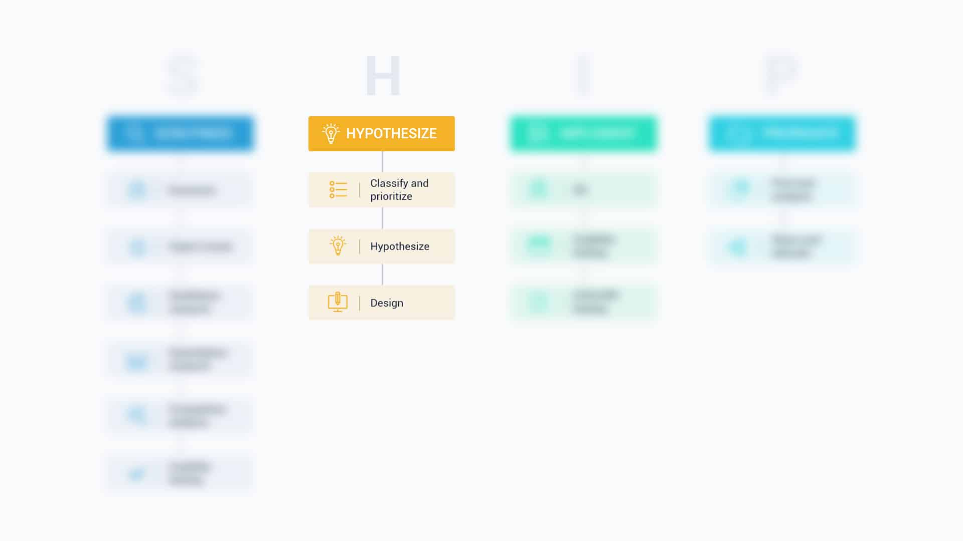
It comes after we have completed the research phase. 

This is an indication that we don’t just pull a hypothesis out of thin air. We always make sure that it is based on research data. 

But having a research-backed hypothesis doesn’t mean that the hypothesis will always be correct. In fact, tons of hypotheses bear inconclusive results or get disproved. 

The main idea of having a hypothesis in marketing experimentation is to help you gain insights – regardless of the testing outcome. 

By the time you finish reading this article, you’ll know: 

• The essential tips on what to do when crafting a hypothesis for marketing experiments
• How a marketing experiment hypothesis works 

How experts develop a solid hypothesis

The basics: marketing experimentation hypothesis.

A hypothesis is a research-based statement that aims to explain an observed trend and create a solution that will improve the result. This statement is an educated, testable prediction about what will happen.

It has to be stated in declarative form and not as a question.

“ If we add magnification info, product video and making virtual mirror buttons, will that improve engagement? ” is not declarative, but “ Improving the experience of product pages by adding magnification info, product video and making virtual mirror buttons will increase engagement ” is.

Here’s a quick example of how a hypothesis should be phrased: 

• Replacing ___ with __ will increase [conversion goal] by [%], because:
• Removing ___ and __ will decrease [conversion goal] by [%], because:
• Changing ___ into __ will not affect [conversion goal], because:
• Improving  ___ by  ___will increase [conversion goal], because: 

As you can see from the above sentences, a good hypothesis is written in clear and simple language. Reading your hypothesis should tell your team members exactly what you thought was going to happen in an experiment.

Another important element of a good hypothesis is that it defines the variables in easy-to-measure terms, like who the participants are, what changes during the testing, and what the effect of the changes will be: 

Example : Let’s say this is our hypothesis: 

Displaying full look items on every “continue shopping & view your bag” pop-up and highlighting the value of having a full look will improve the visibility of a full look, encourage visitors to add multiple items from the same look and that will increase the average order value, quantity with cross-selling by 3% .

Who are the participants : 

Visitors. 

What changes during the testing : 

Displaying full look items on every “continue shopping & view your bag” pop-up and highlighting the value of having a full look…

What the effect of the changes will be:  

Will improve the visibility of a full look, encourage visitors to add multiple items from the same look and that will increase the average order value, quantity with cross-selling by 3% .

Don’t bite off more than you can chew! Answering some scientific questions can involve more than one experiment, each with its own hypothesis. so, you have to make sure your hypothesis is a specific statement relating to a single experiment.

How a Marketing Experimentation Hypothesis Works

Assuming that you have done conversion research and you have identified a list of issues ( UX or conversion-related problems) and potential revenue opportunities on the site. The next thing you’d want to do is to prioritize the issues and determine which issues will most impact the bottom line.

Having ranked the issues you need to test them to determine which solution works best. At this point, you don’t have a clear solution for the problems identified. So, to get better results and avoid wasting traffic on poor test designs, you need to make sure that your testing plan is guided. 

This is where a hypothesis comes into play. 

For each and every problem you’re aiming to address, you need to craft a hypothesis for it – unless the problem is a technical issue that can be solved right away without the need to hypothesize or test. 

One important thing you should note about an experimentation hypothesis is that it can be implemented in different ways.  

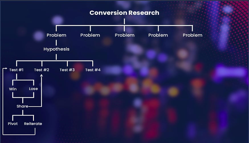
This means that one hypothesis can have four or five different tests as illustrated in the image above. Khalid Saleh , the Invesp CEO, explains: 

“There are several ways that can be used to support one single hypothesis. Each and every way is a possible test scenario. And that means you also have to prioritize the test design you want to start with. Ultimately the name of the game is you want to find the idea that has the biggest possible impact on the bottom line with the least amount of effort. We use almost 18 different metrics to score all of those.”

In one of the recent tests we launched after watching video recordings, viewing heatmaps, and conducting expert reviews, we noticed that:  

• Visitors were scrolling to the bottom of the page to fill out a calculator so as to get a free diet plan. 
• Brand is missing 
• Too many free diet plans – and this made it hard for visitors to choose and understand.  
• No value proposition on the page
• The copy didn’t mention the benefits of the paid program
• There was no clear CTA for the next action

To help you understand, let’s have a look at how the original page looked like before we worked on it: 

So our aim was to make the shopping experience seamless for visitors, make the page more appealing and not confusing. In order to do that, here is how we phrased the hypothesis for the page above: 

Improving the experience of optin landing pages by making the free offer accessible above the fold and highlighting the next action with a clear CTA and will increase the engagement on the offer and increase the conversion rate by 1%.

For this particular hypothesis, we had two design variations aligned to it:

The two above designs are different, but they are aligned to one hypothesis. This goes on to show how one hypothesis can be implemented in different ways. Looking at the two variations above – which one do you think won?

Yes, you’re right, V2 was the winner. 

Considering that there are many ways you can implement one hypothesis, so when you launch a test and it fails, it doesn’t necessarily mean that the hypothesis was wrong. Khalid adds:

“A single failure of a test doesn’t mean that the hypothesis is incorrect. Nine times out of ten it’s because of the way you’ve implemented the hypothesis. Look at the way you’ve coded and look at the copy you’ve used – you are more likely going to find something wrong with it. Always be open.” 

So there are three things you should keep in mind when it comes to marketing experimentation hypotheses: 

• It takes a while for this hypothesis to really fully test it.
• A single failure doesn’t necessarily mean that the hypothesis is incorrect.
• Whether a hypothesis is proved or disproved, you can still learn something about your users.

I know it’s never easy to develop a hypothesis that informs future testing – I mean it takes a lot of intense research behind the scenes, and tons of ideas to begin with. So, I reached out to six CRO experts for tips and advice to help you understand more about developing a solid hypothesis and what to include in it. 

Maurice   says that a solid hypothesis should have not more than one goal: 

Maurice Beerthuyzen – CRO/CXO Lead at ClickValue “Creating a hypothesis doesn’t begin at the hypothesis itself. It starts with research. What do you notice in your data, customer surveys, and other sources? Do you understand what happens on your website? When you notice an opportunity it is tempting to base one single A/B test on one hypothesis. Create hypothesis A and run a single test, and then move forward to the next test. With another hypothesis. But it is very rare that you solve your problem with only one hypothesis. Often a test provides several other questions. Questions which you can solve with running other tests. But based on that same hypothesis! We should not come up with a new hypothesis for every test. Another mistake that often happens is that we fill the hypothesis with multiple goals. Then we expect that the hypothesis will work on conversion rate, average order value, and/or Click Through Ratio. Of course, this is possible, but when you run your test, your hypothesis can only have one goal at once. And what if you have two goals? Just split the hypothesis then create a secondary hypothesis for your second goal. Every test has one primary goal. What if you find a winner on your secondary hypothesis? Rerun the test with the second hypothesis as the primary one.”

Jon believes that a strong hypothesis is built upon three pillars:

Jon MacDonald – President and Founder of The Good Respond to an established challenge – The challenge must have a strong background based on data, and the background should state an established challenge that the test is looking to address. Example: “Sign up form lacks proof of value, incorrectly assuming if users are on the page, they already want the product.” Propose a specific solution – What is the one, the single thing that is believed will address the stated challenge? Example: “Adding an image of the dashboard as a background to the signup form…”. State the assumed impact – The assumed impact should reference one specific, measurable optimization goal that was established prior to forming a hypothesis. Example: “…will increase signups.” So, if your hypothesis doesn’t have a specific, measurable goal like “will increase signups,” you’re not really stating a test hypothesis!”

Matt uses his own hypothesis builder to collate important data points into a single hypothesis. 

Matt Beischel – Founder of Corvus CRO Like Jon, Matt also breaks down his hypothesis writing process into three sections. Unlike Jon, Matt sections are: Comprehension Response Outcome I set it up so that the names neatly match the “CRO.” It’s a sort of “mad-libs” style fill-in-the-blank where each input is an important piece of information for building out a robust hypothesis. I consider these the minimum required data points for a good hypothesis; if you can’t completely fill out the form, then you don’t have a good hypothesis. Here’s a breakdown of each data point: Comprehension – Identifying something that can be improved upon Problem: “What is a problem we have?” Observation Method: “How did we identify the problem?” Response – Change that can cause improvement Variation: “What change do we think could solve the problem?” Location: “Where should the change occur?” Scope: “What are the conditions for the change?” Audience: “Who should the change affect?” Outcome – Measurable result of the change that determines the success Behavior Change : “What change in behavior are we trying to affect?” Primary KPI: “What is the important metric that determines business impact?” Secondary KPIs: “Other metrics that will help reinforce/refute the Primary KPI” Something else to consider is that I have a “user first” approach to formulating hypotheses. My process above is always considered within the context of how it would first benefit the user. Now, I do feel that a successful experiment should satisfy the needs of BOTH users and businesses, but always be in favor of the user. Notice that “Behavior Change” is the first thing listed in Outcome, not primary business KPI. Sure, at the end of the day you are working for the business’s best interests (both strategically and financially), but placing the user first will better inform your decision making and prioritization; there’s a reason that things like personas, user stories, surveys, session replays, reviews, etc. exist after all. A business-first ideology is how you end up with dark patterns and damaging brand credibility.”

One of the many mistakes that CROs make when writing a hypothesis is that they are focused on wins and not on insights. Shiva advises against this mindset:

Shiva Manjunath – Marketing Manager and CRO at Gartner “Test to learn, not test to win. It’s a very simple reframe of hypotheses but can have a magnitude of difference. Here’s an example: Test to Win Hypothesis: If I put a product video in the middle of the product page, I will improve add to cart rates and improve CVR. Test to Learn Hypothesis: If I put a product video on the product page, there will be high engagement with the video and it will positively influence traffic What you’re doing is framing your hypothesis, and test, in a particular way to learn as much as you can. That is where you gain marketing insights. The more you run ‘marketing insight’ tests, the more you will win. Why? The more you compound marketing insight learnings, your win velocity will start to increase as a proxy of the learnings you’ve achieved. Then, you’ll have a higher chance of winning in your tests – and the more you’ll be able to drive business results.”

Lorenzo  says it’s okay to focus on achieving a certain result as long as you are also getting an answer to: “Why is this event happening or not happening?”

Lorenzo Carreri – CRO Consultant “When I come up with a hypothesis for a new or iterative experiment, I always try to find an answer to a question. It could be something related to a problem people have or an opportunity to achieve a result or a way to learn something. The main question I want to answer is “Why is this event happening or not happening?” The question is driven by data, both qualitative and quantitative. The structure I use for stating my hypothesis is: From [data source], I noticed [this problem/opportunity] among [this audience of users] on [this page or multiple pages]. So I believe that by [offering this experiment solution], [this KPI] will [increase/decrease/stay the same].

Jakub Linowski says that hypotheses are meant to hold researchers accountable:

Jakub Linowski – Chief Editor of GoodUI “They do this by making your change and prediction more explicit. A typical hypothesis may be expressed as: If we change (X), then it will have some measurable effect (A). Unfortunately, this oversimplified format can also become a heavy burden to your experiment design with its extreme reductionism. However you decide to format your hypotheses, here are three suggestions for more flexibility to avoid limiting yourself. One Or More Changes To break out of the first limitation, we have to admit that our experiments may contain a single or multiple changes. Whereas the classic hypothesis encourages a single change or isolated variable, it’s not the only way we can run experiments. In the real world, it’s quite normal to see multiple design changes inside a single variation. One valid reason for doing this is when wishing to optimize a section of a website while aiming for a greater effect. As more positive changes compound together, there are times when teams decide to run bigger experiments. An experiment design (along with your hypotheses) therefore should allow for both single or multiple changes. One Or More Metrics A second limitation of many hypotheses is that they often ask us to only make a single prediction at a time. There are times when we might like to make multiple guesses or predictions to a set of metrics. A simple example of this might be a trade-off experiment with a guess of increased sales but decreased trial signups. Being able to express single or multiple metrics in our experimental designs should therefore be possible. Estimates, Directional Predictions, Or Unknowns Finally, traditional hypotheses also tend to force very simple directional predictions by asking us to guess whether something will increase or decrease. In reality, however, the fidelity of predictions can be higher or lower. On one hand, I’ve seen and made experiment estimations that contain specific numbers from prior data (ex: increase sales by 14%). While at other times it should also be acceptable to admit the unknown and leave the prediction blank. One example of this is when we are testing a completely novel idea without any prior data in a highly exploratory type of experiment. In such cases, it might be dishonest to make any sort of predictions and we should allow ourselves to express the unknown comfortably.”

Conclusion 

So there you have it! Before you jump on launching a test, start by making sure that your hypothesis is solid and backed by research. Ask yourself the questions below when crafting a hypothesis for marketing experimentation:

• Is the hypothesis backed by research?
• Can the hypothesis be tested?
• Does the hypothesis provide insights?
• Does the hypothesis set the expectation that there will be an explanation behind the results of whatever you’re testing?

Don’t worry! Hypothesizing may seem like a very complicated process, but it’s not complicated in practice especially when you have done proper research.

If you enjoyed reading this article and you’d love to get the best CRO content – delivered by the best experts in the industry – straight to your inbox, every week. Please subscribe here .

Share This Article

Join 25,000+ marketing professionals.

Subscribe to Invesp’s blog feed for future articles delivered to receive weekly updates by email.

Discover Similar Topics

GA4 Segments: An In-depth Guide with Examples

12 Psychological Tricks to Increase Your Conversion Rate

Our Services

• Conversion Optimization Training
• Conversion Rate Optimization Professional Services
• Landing Page Optimization
• Conversion Rate Audit
• Design for Growth
• Conversion Research & Discovery
• End to End Digital Optimization

By Industry

• E-commerce CRO Services
• Lead Generation CRO Services
• SaaS CRO Services
• Startup CRO Program
• Case Studies
• Privacy Policy
• © 2006-2020 All rights reserved. Invesp

Subscribe with us

• US office: Chicago, IL
• European office: Istanbul, Turkey
• +1.248.270.3325
• [email protected]
• Conversion Rate Optimization Services
• © 2006-2023 All rights reserved. Invesp
• Popular Topics
• A/B Testing
• Business & Growth
• Copywriting
• Infographics
• Landing Pages
• Sales & Marketing

Marketing Research Design & Analysis 2019

5 hypothesis testing.

This chapter is primarily based on Field, A., Miles J., & Field, Z. (2012): Discovering Statistics Using R. Sage Publications, chapters 5, 9, 15, 18 .

You can download the corresponding R-Code here

5.1 Introduction

We test hypotheses because we are confined to taking samples – we rarely work with the entire population. In the previous chapter, we introduced the standard error (i.e., the standard deviation of a large number of hypothetical samples) as an estimate of how well a particular sample represents the population. We also saw how we can construct confidence intervals around the sample mean \(\bar x\) by computing \(SE_{\bar x}\) as an estimate of \(\sigma_{\bar x}\) using \(s\) as an estimate of \(\sigma\) and calculating the 95% CI as \(\bar x \pm 1.96 * SE_{\bar x}\) . Although we do not know the true population mean ( \(\mu\) ), we might have an hypothesis about it and this would tell us how the corresponding sampling distribution looks like. Based on the sampling distribution of the hypothesized population mean, we could then determine the probability of a given sample assuming that the hypothesis is true .

Let us again begin by assuming we know the entire population using the example of music listening times among students from the previous example. As a reminder, the following plot shows the distribution of music listening times in the population of WU students.

In this example, the population mean ( \(\mu\) ) is equal to 19.98, and the population standard deviation \(\sigma\) is equal to 14.15.

5.1.1 The null hypothesis

Let us assume that we were planning to take a random sample of 50 students from this population and our hypothesis was that the mean listening time is equal to some specific value \(\mu_0\) , say \(10\) . This would be our null hypothesis . The null hypothesis refers to the statement that is being tested and is usually a statement of the status quo, one of no difference or no effect. In our example, the null hypothesis would state that there is no difference between the true population mean \(\mu\) and the hypothesized value \(\mu_0\) (in our example \(10\) ), which can be expressed as follows:

\[ H_0: \mu = \mu_0 \] When conducting research, we are usually interested in providing evidence against the null hypothesis. If we then observe sufficient evidence against it and our estimate is said to be significant. If the null hypothesis is rejected, this is taken as support for the alternative hypothesis . The alternative hypothesis assumes that some difference exists, which can be expressed as follows:

\[ H_1: \mu \neq \mu_0 \] Accepting the alternative hypothesis in turn will often lead to changes in opinions or actions. Note that while the null hypothesis may be rejected, it can never be accepted based on a single test. If we fail to reject the null hypothesis, it means that we simply haven’t collected enough evidence against the null hypothesis to disprove it. In classical hypothesis testing, there is no way to determine whether the null hypothesis is true. Hypothesis testing provides a means to quantify to what extent the data from our sample is in line with the null hypothesis.

In order to quantify the concept of “sufficient evidence” we look at the theoretical distribution of the sample means given our null hypothesis and the sample standard error. Using the available information we can infer the sampling distribution for our null hypothesis. Recall that the standard deviation of the sampling distribution (i.e., the standard error of the mean) is given by \(\sigma_{\bar x}={\sigma \over \sqrt{n}}\) , and thus can be computed as follows:

Since we know from the central limit theorem that the sampling distribution is normal for large enough samples, we can now visualize the expected sampling distribution if our null hypothesis was in fact true (i.e., if the was no difference between the true population mean and the hypothesized mean of 10).

We also know that 95% of the probability is within 1.96 standard deviations from the mean. Values higher than that are rather unlikely, if our hypothesis about the population mean was indeed true. This is shown by the shaded area, also known as the “rejection region”. To test our hypothesis that the population mean is equal to \(10\) , let us take a random sample from the population.

The mean listening time in the sample (black line) \(\bar x\) is 18.59. We can already see from the graphic above that such a value is rather unlikely under the hypothesis that the population mean is \(10\) . Intuitively, such a result would therefore provide evidence against our null hypothesis. But how could we quantify specifically how unlikely it is to obtain such a value and decide whether or not to reject the null hypothesis? Significance tests can be used to provide answers to these questions.

5.1.2 Statistical inference on a sample

5.1.2.1 test statistic, 5.1.2.1.1 z-scores.

Let’s go back to the sampling distribution above. We know that 95% of all values will fall within 1.96 standard deviations from the mean. So if we could express the distance between our sample mean and the null hypothesis in terms of standard deviations, we could make statements about the probability of getting a sample mean of the observed magnitude (or more extreme values). Essentially, we would like to know how many standard deviations ( \(\sigma_{\bar x}\) ) our sample mean ( \(\bar x\) ) is away from the population mean if the null hypothesis was true ( \(\mu_0\) ). This can be formally expressed as follows:

\[ \bar x- \mu_0 = z \sigma_{\bar x} \]

In this equation, z will tell us how many standard deviations the sample mean \(\bar x\) is away from the null hypothesis \(\mu_0\) . Solving for z gives us:

\[ z = {\bar x- \mu_0 \over \sigma_{\bar x}}={\bar x- \mu_0 \over \sigma / \sqrt{n}} \]

This standardized value (or “z-score”) is also referred to as a test statistic . Let’s compute the test statistic for our example above:

To make a decision on whether the difference can be deemed statistically significant, we now need to compare this calculated test statistic to a meaningful threshold. In order to do so, we need to decide on a significance level \(\alpha\) , which expresses the probability of finding an effect that does not actually exist (i.e., Type I Error). You can find a detailed discussion of this point at the end of this chapter. For now, we will adopt the widely accepted significance level of 5% and set \(\alpha\) to 0.05. The critical value for the normal distribution and \(\alpha\) = 0.05 can be computed using the qnorm() function as follows:

We use 0.975 and not 0.95 since we are running a two-sided test and need to account for the rejection region at the other end of the distribution. Recall that for the normal distribution, 95% of the total probability falls within 1.96 standard deviations of the mean, so that higher (absolute) values provide evidence against the null hypothesis. Generally, we speak of a statistically significant effect if the (absolute) calculated test statistic is larger than the (absolute) critical value. We can easily check if this is the case in our example:

Since the absolute value of the calculated test statistic is larger than the critical value, we would reject \(H_0\) and conclude that the true population mean \(\mu\) is significantly different from the hypothesized value \(\mu_0 = 10\) .

5.1.2.1.2 t-statistic

You may have noticed that the formula for the z-score above assumes that we know the true population standard deviation ( \(\sigma\) ) when computing the standard deviation of the sampling distribution ( \(\sigma_{\bar x}\) ) in the denominator. However, the population standard deviation is usually not known in the real world and therefore represents another unknown population parameter which we have to estimate from the sample. We saw in the previous chapter that we usually use \(s\) as an estimate of \(\sigma\) and \(SE_{\bar x}\) as and estimate of \(\sigma_{\bar x}\) . Intuitively, we should be more conservative regarding the critical value that we used above to assess whether we have a significant effect to reflect this uncertainty about the true population standard deviation. That is, the threshold for a “significant” effect should be higher to safeguard against falsely claiming a significant effect when there is none. If we replace \(\sigma_{\bar x}\) by it’s estimate \(SE_{\bar x}\) in the formula for the z-score, we get a new test statistic (i.e, the t-statistic ) with its own distribution (the t-distribution ):

\[ t = {\bar x- \mu_0 \over SE_{\bar x}}={\bar x- \mu_0 \over s / \sqrt{n}} \]

Here, \(\bar X\) denotes the sample mean and \(s\) the sample standard deviation. The t-distribution has more probability in its “tails”, i.e. farther away from the mean. This reflects the higher uncertainty introduced by replacing the population standard deviation by its sample estimate. Intuitively, this is particularly relevant for small samples, since the uncertainty about the true population parameters decreases with increasing sample size. This is reflected by the fact that the exact shape of the t-distribution depends on the degrees of freedom , which is the sample size minus one (i.e., \(n-1\) ). To see this, the following graph shows the t-distribution with different degrees of freedom for a two-tailed test and \(\alpha = 0.05\) . The grey curve shows the normal distribution.

Notice that as \(n\) gets larger, the t-distribution gets closer and closer to the normal distribution, reflecting the fact that the uncertainty introduced by \(s\) is reduced. To summarize, we now have an estimate for the standard deviation of the distribution of the sample mean (i.e., \(SE_{\bar x}\) ) and an appropriate distribution that takes into account the necessary uncertainty (i.e., the t-distribution). Let us now compute the t-statistic according to the formula above:

Notice that the value of the t-statistic is higher compared to the z-score (4.29). This can be attributed to the fact that by using the \(s\) as and estimate of \(\sigma\) , we underestimate the true population standard deviation. Hence, the critical value would need to be larger to adjust for this. This is what the t-distribution does. Let us compute the critical value from the t-distribution with n - 1 degrees of freedom.

Again, we use 0.975 and not 0.95 since we are running a two-sided test and need to account for the rejection region at the other end of the distribution. Notice that the new critical value based on the t-distributionis larger, to reflect the uncertainty when estimating \(\sigma\) from \(s\) . Now we can see that the calculated test statistic is still larger than the critical value.

The following graphics shows that the calculated test statistic (red line) falls into the rejection region so that in our example, we would reject the null hypothesis that the true population mean is equal to \(10\) .

Decision: Reject \(H_0\) , given that the calculated test statistic is larger than critical value.

Something to keep in mind here is the fact the test statistic is a function of the sample size. This, as \(n\) gets large, the test statistic gets larger as well and we are more likely to find a significant effect. This reflects the decrease in uncertainty about the true population mean as our sample size increases.

5.1.2.2 P-values

In the previous section, we computed the test statistic, which tells us how close our sample is to the null hypothesis. The p-value corresponds to the probability that the test statistic would take a value as extreme or more extreme than the one that we actually observed, assuming that the null hypothesis is true . It is important to note that this is a conditional probability : we compute the probability of observing a sample mean (or a more extreme value) conditional on the assumption that the null hypothesis is true. The pnorm() function can be used to compute this probability. It is the cumulative probability distribution function of the `normal distribution. Cumulative probability means that the function returns the probability that the test statistic will take a value less than or equal to the calculated test statistic given the degrees of freedom. However, we are interested in obtaining the probability of observing a test statistic larger than or equal to the calculated test statistic under the null hypothesis (i.e., the p-value). Thus, we need to subtract the cumulative probability from 1. In addition, since we are running a two-sided test, we need to multiply the probability by 2 to account for the rejection region at the other side of the distribution.

This value corresponds to the probability of observing a mean equal to or larger than the one we obtained from our sample, if the null hypothesis was true. As you can see, this probability is very low. A small p-value signals that it is unlikely to observe the calculated test statistic under the null hypothesis. To decide whether or not to reject the null hypothesis, we would now compare this value to the level of significance ( \(\alpha\) ) that we chose for our test. For this example, we adopt the widely accepted significance level of 5%, so any test results with a p-value < 0.05 would be deemed statistically significant. Note that the p-value is directly related to the value of the test statistic. The relationship is such that the higher (lower) the value of the test statistic, the lower (higher) the p-value.

Decision: Reject \(H_0\) , given that the p-value is smaller than 0.05.

5.1.2.3 Confidence interval

For a given statistic calculated for a sample of observations (e.g., listening times), a 95% confidence interval can be constructed such that in 95% of samples, the true value of the true population mean will fall within its limits. If the parameter value specified in the null hypothesis (here \(10\) ) does not lie within the bounds, we reject \(H_0\) . Building on what we learned about confidence intervals in the previous chapter, the 95% confidence interval based on the t-distribution can be computed as follows:

\[ CI_{lower} = {\bar x} - t_{1-{\alpha \over 2}} * SE_{\bar x} \\ CI_{upper} = {\bar x} + t_{1-{\alpha \over 2}} * SE_{\bar x} \]

It is easy to compute this interval manually:

The interpretation of this interval is as follows: if we would (hypothetically) take 100 samples and calculated the mean and confidence interval for each of them, then the true population mean would be included in 95% of these intervals. The CI is informative when reporting the result of your test, since it provides an estimate of the uncertainty associated with the test result. From the test statistic or the p-value alone, it is not easy to judge in which range the true population parameter is located. The CI provides an estimate of this range.

Decision: Reject \(H_0\) , given that the parameter value from the null hypothesis ( \(10\) ) is not included in the interval.

To summarize, you can see that we arrive at the same conclusion (i.e., reject \(H_0\) ), irrespective if we use the test statistic, the p-value, or the confidence interval. However, keep in mind that rejecting the null hypothesis does not prove the alternative hypothesis (we can merely provide support for it). Rather, think of the p-value as the chance of obtaining the data we’ve collected assuming that the null hypothesis is true. You should report the confidence interval to provide an estimate of the uncertainty associated with your test results.

5.1.3 Choosing the right test

The test statistic, as we have seen, measures how close the sample is to the null hypothesis and often follows a well-known distribution (e.g., normal, t, or chi-square). To select the correct test, various factors need to be taken into consideration. Some examples are:

• On what scale are your variables measured (categorical vs. continuous)?
• Do you want to test for relationships or differences?
• If you test for differences, how many groups would you like to test?
• For parametric tests, are the assumptions fulfilled?

The previous discussion used a one sample t-test as an example, which requires that variable is measured on an interval or ratio scale. If you are confronted with other settings, the following flow chart provides a rough guideline on selecting the correct test:

Flowchart for selecting an appropriate test (source: McElreath, R. (2016): Statistical Rethinking, p. 2)

For a detailed overview over the different type of tests, please also refer to this overview by the UCLA.

5.1.3.1 Parametric vs. non-parametric tests

A basic distinction can be made between parametric and non-parametric tests. Parametric tests require that variables are measured on an interval or ratio scale and that the sampling distribution follows a known distribution. Non-Parametric tests on the other hand do not require the sampling distribution to be normally distributed (a.k.a. “assumption free tests”). These tests may be used when the variable of interest is measured on an ordinal scale or when the parametric assumptions do not hold. They often rely on ranking the data instead of analyzing the actual scores. By ranking the data, information on the magnitude of differences is lost. Thus, parametric tests are more powerful if the sampling distribution is normally distributed. In this chapter, we will first focus on parametric tests and cover non-parametric tests later.

5.1.3.2 One-tailed vs. two-tailed test

For some tests you may choose between a one-tailed test versus a two-tailed test . The choice depends on the hypothesis you specified, i.e., whether you specified a directional or a non-directional hypotheses. In the example above, we used a non-directional hypothesis . That is, we stated that the mean is different from the comparison value \(\mu_0\) , but we did not state the direction of the effect. A directional hypothesis states the direction of the effect. For example, we might test whether the population mean is smaller than a comparison value:

\[ H_0: \mu \ge \mu_0 \\ H_1: \mu < \mu_0 \]

Similarly, we could test whether the population mean is larger than a comparison value:

\[ H_0: \mu \le \mu_0 \\ H_1: \mu > \mu_0 \]

Connected to the decision of how to phrase the hypotheses (directional vs. non-directional) is the choice of a one-tailed test versus a two-tailed test . Let’s first think about the meaning of a one-tailed test. Using a significance level of 0.05, a one-tailed test means that 5% of the total area under the probability distribution of our test statistic is located in one tail. Thus, under a one-tailed test, we test for the possibility of the relationship in one direction only, disregarding the possibility of a relationship in the other direction. In our example, a one-tailed test could test either if the mean listening time is significantly larger or smaller compared to the control condition, but not both. Depending on the direction, the mean listening time is significantly larger (smaller) if the test statistic is located in the top (bottom) 5% of its probability distribution.

The following graph shows the critical values that our test statistic would need to surpass so that the difference between the population mean and the comparison value would be deemed statistically significant.

It can be seen that under a one-sided test, the rejection region is at one end of the distribution or the other. In a two-sided test, the rejection region is split between the two tails. As a consequence, the critical value of the test statistic is smaller using a one-tailed test, meaning that it has more power to detect an effect. Having said that, in most applications, we would like to be able catch effects in both directions, simply because we can often not rule out that an effect might exist that is not in the hypothesized direction. For example, if we would conduct a one-tailed test for a mean larger than some specified value but the mean turns out to be substantially smaller, then testing a one-directional hypothesis ($H_0: _0 $) would not allow us to conclude that there is a significant effect because there is not rejection at this end of the distribution.

5.1.4 Summary

As we have seen, the process of hypothesis testing consists of various steps:

• Formulate null and alternative hypotheses
• Select an appropriate test
• Choose the level of significance ( \(\alpha\) )
• Descriptive statistics and data visualization
• Conduct significance test
• Report results and draw a marketing conclusion

In the following, we will go through the individual steps using examples for different tests.

5.2 One sample t-test

The example we used in the introduction was an example of the one sample t-test and we computed all statistics by hand to explain the underlying intuition. When you conduct hypothesis tests using R, you do not need to calculate these statistics by hand, since there are build-in routines to conduct the steps for you. Let us use the same example again to see how you would conduct hypothesis tests in R.

1. Formulate null and alternative hypotheses

The null hypothesis states that there is no difference between the true population mean \(\mu\) and the hypothesized value (i.e., \(10\) ), while the alternative hypothesis states the opposite:

\[ H_0: \mu = 10 \\ H_1: \mu \neq 10 \]

2. Select an appropriate test

Because we would like to test if the mean of a variable is different from a specified threshold, the one-sample t-test is appropriate. The assumptions of the test are 1) that the variable is measured using an interval or ratio scale, and 2) that the sampling distribution is normal. Both assumptions are met since 1) listening time is a ratio scale, and 2) we deem the sample size (n = 50) large enough to assume a normal sampling distribution according to the central limit theorem.

3. Choose the level of significance

We choose the conventional 5% significance level.

4. Descriptive statistics and data visualization

Provide descriptive statistics using the stat.desc() function:

From this, we can already see that the mean is different from the hypothesized value. The question however remains, whether this difference is significantly different, given the sample size and the variability in the data. Since we only have one continuous variable, we can visualize the distribution in a histogram.

5. Conduct significance test

In the beginning of the chapter, we saw, how you could conduct significance test by hand. However, R has built-in routines that you can use to conduct the analyses. The t.test() function can be used to conduct the test. To test if the listening time among WU students was 10, you can use the following code:

Note that if you would have stated a directional hypothesis (i.e., the mean is either greater or smaller than 10 hours), you could easily amend the code to conduct a one sided test by changing the argument alternative from 'two.sided' to either 'less' or 'greater' .

6. Report results and draw a marketing conclusion

Note that the results are the same as above, when we computed the test by hand. You could summarize the results as follows:

On average, the listening times in our sample were different form 10 hours per month (Mean = 18.99 hours, SE = 1.78). This difference was significant t(49) = 5.058, p < .05 (95% CI = [15.42; 22.56]). Based on this evidence, we can conclude that the mean in our sample is significantly lower compared to the hypothesized population mean of \(10\) hours, providing evidence against the null hypothesis.

Note that in the reporting above, the number 49 in parenthesis refers to the degrees of freedom that are available from the output.

5.3 Comparing two means

In the one-sample test above, we tested the hypothesis that the population mean has some specific value \(\mu_0\) using data from only one sample. In marketing (as in many other disciplines), you will often be confronted with a situation where you wish to compare the means of two groups. For example, you may conduct an experiment and randomly split your sample into two groups, one of which receives a treatment (experimental group) while the other doesn’t (control group). In this case, the units (e.g., participants, products) in each group are different (‘between-subjects design’) and the samples are said to be independent. Hence, we would use a independent-means t-test . If you run an experiment with two experimental conditions and the same units (e.g., participants, products) were observed in both experimental conditions, the sample is said to be dependent in the sense that you have the same units in each group (‘within-subjects design’). In this case, we would need to conduct an dependent-means t-test . Both tests are described in the following sections, beginning with the independent-means t-test.

5.3.1 Independent-means t-test

Using an independent-means t-test, we can compare the means of two possibly different populations. It is, for example, quite common for online companies to test new service features by running an experiment and randomly splitting their website visitors into two groups: one is exposed to the website with the new feature (experimental group) and the other group is not exposed to the new feature (control group). This is a typical A/B-Test scenario.

As an example, imagine that a music streaming service would like to introduce a new playlist feature that let’s their users access playlists created by other users. The goal is to analyse how the new service feature impacts the listening time of users. The service randomly splits a representative subset of their users into two groups and collects data about their listening times over one month. Let’s create a data set to simulate such a scenario.

This data set contains two variables: the variable hours indicates the music listening times (in hours) and the variable group indicates from which group the observation comes, where ‘A’ refers to the control group (with the standard service) and ‘B’ refers to the experimental group (with the new playlist feature). Let’s first look at the descriptive statistics by group using the describeBy function:

From this, we can already see that there is a difference in means between groups A and B. We can also see that the number of observations is different, as is the standard deviation. The question that we would like to answer is whether there is a significant difference in mean listening times between the groups. Remember that different users are contained in each group (‘between-subjects design’) and that the observations in one group are independent of the observations in the other group. Before we will see how you can easily conduct an independent-means t-test, let’s go over some theory first.

5.3.1.1 Theory

As a starting point, let us label the unknown population mean of group A (control group) in our experiment \(\mu_1\) , and that of group B (experimental group) \(\mu_2\) . In this setting, the null hypothesis would state that the mean in group A is equal to the mean in group B:

\[ H_0: \mu_1=\mu_2 \]

This is equivalent to stating that the difference between the two groups ( \(\delta\) ) is zero:

\[ H_0: \mu_1 - \mu_2=0=\delta \]

That is, \(\delta\) is the new unknown population parameter, so that the null and alternative hypothesis become:

\[ H_0: \delta = 0 \\ H_1: \delta \ne 0 \]

Remember that we usually don’t have access to the entire population so that we can not observe \(\delta\) and have to estimate is from a sample statistic, which we define as \(d = \bar x_1-\bar x_2\) , i.e., the difference between the sample means from group a ( \(\bar x_1\) ) and group b ( \(\bar x_2\) ). But can we really estimate \(d\) from \(\delta\) ? Remember from the previous chapter, that we could estimate \(\mu\) from \(\bar x\) , because if we (hypothetically) take a larger number of samples, the distribution of the means of these samples (the sampling distribution) will be normally distributed and its mean will be (in the limit) equal to the population mean. It turns out that we can use the same underlying logic here. The above samples were drawn from two different populations with \(\mu_1\) and \(\mu_2\) . Let us compute the difference in means between these two populations:

This means that the true difference between the mean listening times of groups a and b is -7.42. Let us now repeat the exercise from the previous chapter: let us repeatedly draw a large number of \(20,000\) random samples of 100 users from each of these populations, compute the difference (i.e., \(d\) , our estimate of \(\delta\) ), store the difference for each draw and create a histogram of \(d\) .

This gives us the sampling distribution of the mean differences between the samples. You will notice that this distribution follows a normal distribution and is centered around the true difference between the populations. This means that, on average, the difference between two sample means \(d\) is a good estimate of \(\delta\) . In our example, the difference between \(\bar x_1\) and \(\bar x_2\) is:

Now that we have \(d\) as an estimate of \(\delta\) , how can we find out if the observed difference is significantly different from the null hypothesis (i.e., \(\delta = 0\) )?

Recall from the previous section, that the standard deviation of the sampling distribution \(\sigma_{\bar x}\) (i.e., the standard error) gives us indication about the precision of our estimate. Further recall that the standard error can be calculated as \(\sigma_{\bar x}={\sigma \over \sqrt{n}}\) . So how can we calculate the standard error of the difference between two population means? According to the variance sum law , to find the variance of the sampling distribution of differences, we merely need to add together the variances of the sampling distributions of the two populations that we are comparing. To find the standard error, we only need to take the square root of the variance (because the standard error is the standard deviation of the sampling distribution and the standard deviation is the square root of the variance), so that we get:

\[ \sigma_{\bar x_1-\bar x_2} = \sqrt{{\sigma_1^2 \over n_1}+{\sigma_2^2 \over n_2}} \]

But recall that we don’t actually know the true population standard deviation, so we use \(SE_{\bar x_1-\bar x_2}\) as an estimate of \(\sigma_{\bar x_1-\bar x_2}\) :

\[ SE_{\bar x_1-\bar x_2} = \sqrt{{s_1^2 \over n_1}+{s_2^2 \over n_2}} \]

Hence, for our example, we can calculate the standard error as follows:

Recall from above that we can calculate the t-statistic as:

\[ t= {\bar x - \mu_0 \over {s \over \sqrt{n}}} \]

Exchanging \(\bar x\) for \(d\) , we get

\[ t= {(\bar{x}_1 - \bar{x}_2) - (\mu_1 - \mu_2) \over {\sqrt{{s_1^2 \over n_1}+{s_2^2 \over n_2}}}} \]

Note that according to our hypothesis \(\mu_1-\mu_2=0\) , so that we can calculate the t-statistic as:

Following the example of our one sample t-test above, we would now need to compare this calculated test statistic to a critical value in order to assess if \(d\) is sufficiently far away from the null hypothesis to be statistically significant. To do this, we would need to know the exact t-distribution, which depends on the degrees of freedom. The problem is that deriving the degrees of freedom in this case is not that obvious. If we were willing to assume that \(\sigma_1=\sigma_2\) , the correct t-distribution has \(n_1 -1 + n_2-1\) degrees of freedom (i.e., the sum of the degrees of freedom of the two samples). However, because in real life we don not know if \(\sigma_1=\sigma_2\) , we need to account for this additional uncertainty. We will not go into detail here, but R automatically uses a sophisticated approach to correct the degrees of freedom called the Welch’s correction, as we will see in the subsequent application.

5.3.1.2 Application

The section above explained the theory behind the independent-means t-test and showed how to compute the statistics manually. Obviously you don’t have to compute these statistics by hand in this section shows you how to conduct an independent-means t-test in R using the example from above.

We wish to analyze whether there is a significant difference in music listening times between groups A and B. So our null hypothesis is that the means from the two populations are the same (i.e., there is no difference), while the alternative hypothesis states the opposite:

\[ H_0: \mu_1=\mu_2\\ H_1: \mu_1 \ne \mu_2 \]

Since we have a ratio scaled variable (i.e., listening times) and two independent groups, where the mean of one sample is independent of the group of the second sample (i.e., the groups contain different units), the independent-means t-test is appropriate.

We can compute the descriptive statistics for each group separately, using the describeBy() function:

This already shows us that the mean between groups A and B are different. We can visualize the data using a plot of means, boxplot, and a histogram.

To conduct the independent means t-test, we can use the t.test() function:

The results showed that listening times were higher in the experimental group B (Mean = 28.50, SE = 1.7) compared to the control group (Mean = 18.11, SE = 1.22). This means that the listening times were 10.39 hours higher on average in the experimental group (B), compared to the control group (A). An independent-means t-test showed that this difference is significant t(195.73) = -4.9646, p < .05 (95% CI = [-14.514246,-6.261264]).

5.3.2 Dependent-means t-test

While the independent-means t-test is used when different units (e.g., participants, products) were assigned to the different condition, the dependent-means t-test is used when there are two experimental conditions and the same units (e.g., participants, products) were observed in both experimental conditions.

Imagine, for example, a slightly different experimental setup for the above experiment. Imagine that we do not assign different users to the groups, but that a sample of 100 users gets to use the music streaming service with the new feature for one month and we compare the music listening times of these users during the month of the experiment with the listening time in the previous month. Let us generate data for this example:

Note that the data set has almost the same structure as before only that we know have two variables representing the listening times of each user in the month before the experiment and during the month of the experiment when the new feature was tested.

5.3.2.1 Theory

In this case, we want to test the hypothesis that there is no difference in mean the mean listening times between the two months. This can be expressed as follows:

\[ H_0: \mu_D = 0 \\ \] Note that the hypothesis only refers to one population, since both observations come from the same units (i.e., users). To use consistent notation, we replace \(\mu_D\) with \(\delta\) and get:

\[ H_0: \delta = 0 \\ H_1: \delta \neq 0 \]

where \(\delta\) denotes the difference between the observed listening times from the two consecutive months of the same users . As is the previous example, since we do not observe the entire population, we estimate \(\delta\) based on the sample using \(d\) , which is the difference in mean listening time between the two months for our sample. Note that we assume that everything else (e.g., number of new releases) remained constant over the two month to keep it simple. We can show as above that the sampling distribution follows a normal distribution with a mean that is (in the limit) the same as the population mean. This means, again, that the difference in sample means is a good estimate for the difference in population means. Let’s compute a new variable \(d\) , which is the difference between two month.

Note that we now have a new variable, which is the difference in listening times (in hours) between the two months. The mean of this difference is:

Again, we use \(SE_{\bar x}\) as an estimate of \(\sigma_{\bar x}\) :

\[ SE_{\bar d}={s \over \sqrt{n}} \] Hence, we can compute the standard error as:

The test statistic is therefore:

\[ t = {\bar d- \mu_0 \over SE_{\bar d}} \] on 99 (i.e., n-1) degrees of freedom. Now we can compute the t-statistic as follows:

Note that in the case of the dependent-means t-test, we only base our hypothesis on one population and hence there is only one population variance. This is because in the dependent sample test, the observations come from the same observational units (i.e., users). Hence, there is no unsystematic variation due to potential differences between users that were assigned to the experimental groups. This means that the influence of unobserved factors (unsystematic variation) relative to the variation due to the experimental manipulation (systematic variation) is not as strong in the dependent-means test compared to the independent-means test and we don’t need to correct for differences in the population variances.

5.3.2.2 Application

Again, we don’t have to compute all this by hand since the t.test(...) function can be used to do it for us. Now we have to use the argument paired=TRUE to let R know that we are working with dependent observations.

We would like to the test if there is a difference in music listening times between the two consecutive months, so our null hypothesis is that there is no difference, while the alternative hypothesis states the opposite:

\[ H_0: \mu_D = 0 \\ H_0: \mu_D \ne 0 \]

Since we have a ratio scaled variable (i.e., listening times) and two observations of the same group of users (i.e., the groups contain the same units), the dependent-means t-test is appropriate.

We can compute the descriptive statistics for each month separately, using the describe() function:

This already shows us that the mean between the two months are different. We can visiualize the data using a plot of means, boxplot, and a histogram.

To plot the data, we need to do some restructuring first, since the variables are now stored in two different columns (“hours_a” and “hours_b”). This is also known as the “wide” format. To plot the data we need all observations to be stored in one variable. This is also known as the “long” format. We can use the melt(...) function from the reshape2 package to “melt” the two variable into one column to plot the data.

Now we are ready to plot the data:

To conduct the independent means t-test, we can use the t.test() function with the argument paired = TRUE :

On average, the same users used the service more when it included the new feature (M = 25.96, SE = 1.68) compared to the service without the feature (M = 20.99, SE = 1.34). This difference was significant t(99) = 2.3781, p < .05 (95% CI = [0.82, 9.12]).

5.3.3 Further considerations

5.3.3.1 type i and type ii errors.

When choosing the level of significance ( \(\alpha\) ). It is important to note that the choice of the significance level affects the type 1 and type 2 error:

• Type I error: When we believe there is a genuine effect in our population, when in fact there isn’t. Probability of type I error ( \(\alpha\) ) = level of significance.
• Type II error: When we believe that there is no effect in the population, when in fact there is.

This following table shows the possible outcomes of a test (retain vs. reject \(H_0\) ), depending on whether \(H_0\) is true or false in reality.

5.3.3.2 Significance level, sample size, power, and effect size

When you plan to conduct an experiment, there are some factors that are under direct control of the researcher:

• Significance level ( \(\alpha\) ) : The probability of finding an effect that does not genuinely exist.
• Sample size (n) : The number of observations in each group of the experimental design.

Unlike α and n, which are specified by the researcher, the magnitude of β depends on the actual value of the population parameter. In addition, β is influenced by the effect size (e.g., Cohen’s d), which can be used to determine a standardized measure of the magnitude of an observed effect. The following parameters are affected more indirectly:

• Power (1-β) : The probability of finding an effect that does genuinely exists.
• Effect size (d) : Standardized measure of the effect size under the alternate hypothesis.

Although β is unknown, it is related to α. For example, if we would like to be absolutely sure that we do not falsely identify an effect which does not exist (i.e., make a type I error), this means that the probability of identifying an effect that does exist (i.e., 1-β) decreases and vice versa. Thus, an extremely low value of α (e.g., α = 0.0001) will result in intolerably high β errors. A common approach is to set α=0.05 and 1-β=0.80.

Unlike the t-value of our test, the effect size (d) is unaffected by the sample size and can be categorized as follows (see Cohen, J. 1988):

• 0.2 (small effect)
• 0.5 (medium effect)
• 0.8 (large effect)

In order to test more subtle effects (smaller effect sizes), you need a larger sample size compared to the test of more obvious effects. In this paper , you can find a list of examples for different effect sizes and the number of observations you need to reliably find an effect of that magnitude. Although the exact effect size is unknown before the experiment, you might be able to make a guess about the effect size (e.g., based on previous studies).

If you wish to obtain a standardized measure of the effect, you may compute the effect size (Cohen’s d) using the cohensD() function from the lsr package. Using the examples from the independent-means t-test above, we would use:

According to the thresholds defined above, this effect would be judged to be a small-medium effect.

For the dependent-means t-test, we would use:

According to the thresholds defined above, this effect would also be judged to be a small-medium effect.

When constructing an experimental design, your goal should be to maximize the power of the test while maintaining an acceptable significance level and keeping the sample as small as possible. To achieve this goal, you may use the pwr package, which let’s you compute n , d , alpha , and power . You only need to specify three of the four input variables to get the fourth.

For example, what sample size do we need (per group) to identify an effect with d = 0.6, α = 0.05, and power = 0.8:

Or we could ask, what is the power of our test with 51 observations in each group, d = 0.6, and α = 0.05:

5.3.3.3 P-values, stopping rules and p-hacking

From my experience, students tend to place a lot of weight on p-values when interpreting their research findings. It is therefore important to note some points that hopefully help to put the meaning of a “significant” vs. “insignificant” test result into perspective.

Significant result

• Even if the probability of the effect being a chance result is small (e.g., less than .05) it doesn’t necessarily mean that the effect is important.
• Very small and unimportant effects can turn out to be statistically significant if the sample size is large enough.

Insignificant result

• If the probability of the effect occurring by chance is large (greater than .05), the alternative hypothesis is rejected. However, this does not mean that the null hypothesis is true.
• Although an effect might not be large enough to be anything other than a chance finding, it doesn’t mean that the effect is zero.
• In fact, two random samples will always have slightly different means that would deemed to be statistically significant if the samples were large enough.

Thus, you should not base your research conclusion on p-values alone!

It is also crucial to determine the sample size before you run the experiment or before you start your analysis. Why? Consider the following example:

• You run an experiment
• After each respondent you analyze the data and look at the mean difference between the two groups with a t-test
• You stop when you have a significant effect

This is called p-hacking and should be avoided at all costs. Assuming that both groups come from the same population (i.e., there is no difference in the means): What is the likelihood that the result will be significant at some point? In other words, what is the likelihood that you will draw the wrong conclusion from your data that there is an effect, while there is none? This is shown in the following graph using simulated data - the color red indicates significant test results that arise although there is no effect (i.e., false positives).

Figure 5.1: p-hacking (red indicates false positives)

5.4 Comparing several means

This chapter is primarily based on Field, A., Miles J., & Field, Z. (2012): Discovering Statistics Using R. Sage Publications, chapters 10 & 12 .

5.4.1 Introduction

In the previous section we learned how to compare means using a t-test. The t-test has some limitations since it only lets you compare 2 means and you can only use it with one independent variable. However, often we would like to compare means from 3 or more groups. In addition, there may be instances in which you manipulate more than one independent variable. For these applications, ANOVA (ANalysis Of VAriance) can be used. Hence, to conduct ANOVA you need:

• A metric dependent variable (i.e., measured using an interval or ratio scale)
• One or more non-metric (categorical) independent variables (also called factors)

A treatment is a particular combination of factor levels, or categories. One-way ANOVA is used when there is only one categorical variable (factor). In this case, a treatment is the same as a factor level. N-way ANOVA is used with two or more factors. Note that we are only going to talk about a single independent variable in the context of ANOVA. If you have multiple independent variables please refere to the chapter on Regression .

Let’s use an example to see how ANOVA works. Similar to the previous example it is also imaginable that the music streaming service experiments with a recommendation system for user created playlists. We now have three groups, the control group “A” with the current system, treatment group “B” who have access to playlists created by other users but are not shown recommendations and treatment group “C” who are shown recommendations for user created playlists. As always, we load and inspect the data first:

The null hypothesis, typically, is that all means are equal (non-directional hypothesis). Hence, in our case:

\[H_0: \mu_1 = \mu_2 = \mu_3\]

The alternative hypothesis is simply that the means are not all equal, i.e.,

\[H_1: \textrm{Means are not all equal}\]

If you wanted to put this in mathematical notation, you could also write:

\[H_1: \exists {i,j}: {\mu_i \ne \mu_j} \]

To get a first impression if there are any differences in listening times across the experimental groups, we use the describeBy(...) function from the psych package:

In addition, you should visualize the data using appropriate plots:

Figure 5.2: Plot of means

Note that ANOVA is an omnibus test, which means that we test for an overall difference between groups. Hence, the test will only tell you if the group means are different, but it won’t tell you exactly which groups are different from another.

So why don’t we then just conduct a series of t-tests for all combinations of groups (i.e., A vs. B, A vs. C, B vs. C)? The reason is that if we assume each test to be independent, then there is a 5% probability of falsely rejecting the null hypothesis (Type I error) for each test. In our case:

• A vs. B (α = 0.05)
• A vs. C (α = 0.05)
• B vs. C (α = 0.05)

This means that the overall probability of making a Type I error is 1-(0.95 3 ) = 0.143, since the probability of no Type I error is 0.95 for each of the three tests. Consequently, the Type I error probability would be 14.3%, which is above the conventional standard of 5%. This is also known as the family-wise or experiment-wise error.

5.4.2 Decomposing variance

The basic concept underlying ANOVA is the decomposition of the variance in the data. There are three variance components which we need to consider:

• We calculate how much variability there is between scores: Total sum of squares (SS T )
• We then calculate how much of this variability can be explained by the model we fit to the data (i.e., how much variability is due to the experimental manipulation): Model sum of squares (SS M )
• … and how much cannot be explained (i.e., how much variability is due to individual differences in performance): Residual sum of squares (SS R )

The following figure shows the different variance components using a generalized data matrix:

Decomposing variance

The total variation is determined by the variation between the categories (due to our experimental manipulation) and the within-category variation that is due to extraneous factors (e.g., promotion of artists on a social network):

\[SS_T= SS_M+SS_R\]

To get a better feeling how this relates to our data set, we can look at the data in a slightly different way. Specifically, we can use the dcast(...) function from the reshape2 package to convert the data to wide format:

In this example, X 1 from the generalized data matrix above would refer to the factor level “A”, X 2 to the level “B”, and X 3 to the level “C”. Y 11 refers to the first data point in the first row (i.e., “13”), Y 12 to the second data point in the first row (i.e., “21”), etc.. The grand mean ( \(\overline{Y}\) ) and the category means ( \(\overline{Y}_c\) ) can be easily computed:

To see how each variance component can be derived, let’s look at the data again. The following graph shows the individual observations by experimental group:

Figure 5.3: Sum of Squares

5.4.2.1 Total sum of squares

To compute the total variation in the data, we consider the difference between each observation and the grand mean. The grand mean is the mean over all observations in the data set. The vertical lines in the following plot measure how far each observation is away from the grand mean:

Figure 5.4: Total Sum of Squares

The formal representation of the total sum of squares (SS T ) is:

\[ SS_T= \sum_{i=1}^{N} (Y_i-\bar{Y})^2 \]

This means that we need to subtract the grand mean from each individual data point, square the difference, and sum up over all the squared differences. Thus, in our example, the total sum of squares can be calculated as:

\[ \begin{align} SS_T =&(13−24.67)^2 + (14−24.67)^2 + … + (2−24.67)^2\\ &+(21−24.67)^2 + (18-24.67)^2 + … + (17−24.67)^2\\ &+(30−24.67)^2 + (37−24.67)^2 + … + (28−24.67)^2\\ &=30855.64 \end{align} \]

You could also compute this in R using:

For the subsequent analyses, it is important to understand the concept behind the degrees of freedom . Remember that in order to estimate a population value from a sample, we need to hold something in the population constant. In ANOVA, the df are generally one less than the number of values used to calculate the SS. For example, when we estimate the population mean from a sample, we assume that the sample mean is equal to the population mean. Then, in order to estimate the population mean from the sample, all but one scores are free to vary and the remaining score needs to be the value that keeps the population mean constant. In our example, we used all 300 observations to calculate the sum of square, so the total degrees of freedom (df T ) are:

\[\begin{equation} \begin{split} df_T = N-1=300-1=299 \end{split} \tag{5.1} \end{equation}\]

5.4.2.2 Model sum of squares

Now we know that there are 26646.33 units of total variation in our data. Next, we compute how much of the total variation can be explained by the differences between groups (i.e., our experimental manipulation). To compute the explained variation in the data, we consider the difference between the values predicted by our model for each observation (i.e., the group mean) and the grand mean. The group mean refers to the mean value within the experimental group. The vertical lines in the following plot measure how far the predicted value for each observation (i.e., the group mean) is away from the grand mean:

Figure 5.5: Model Sum of Squares

The formal representation of the model sum of squares (SS M ) is:

\[ SS_M= \sum_{j=1}^{c} n_j(\bar{Y}_j-\bar{Y})^2 \]

where c denotes the number of categories (experimental groups). This means that we need to subtract the grand mean from each group mean, square the difference, and sum up over all the squared differences. Thus, in our example, the model sum of squares can be calculated as:

\[ \begin{align} SS_M &= 100*(15.47−24.67)^2 + 100*(24.88−24.67)^2 + 100*(33.66−24.67)^2 \\ &= 21321.21 \end{align} \]

You could also compute this manually in R using:

In this case, we used the three group means to calculate the sum of squares, so the model degrees of freedom (df M ) are:

\[ df_M= c-1=3-1=2 \]

5.4.2.3 Residual sum of squares

Lastly, we calculate the amount of variation that cannot be explained by our model. In ANOVA, this is the sum of squared distances between what the model predicts for each data point (i.e., the group means) and the observed values. In other words, this refers to the amount of variation that is caused by extraneous factors, such as differences between product characteristics of the products in the different experimental groups. The vertical lines in the following plot measure how far each observation is away from the group mean:

Figure 5.6: Residual Sum of Squares

The formal representation of the residual sum of squares (SS R ) is:

\[ SS_R= \sum_{j=1}^{c} \sum_{i=1}^{n} ({Y}_{ij}-\bar{Y}_{j})^2 \]

This means that we need to subtract the group mean from each individual observation, square the difference, and sum up over all the squared differences. Thus, in our example, the model sum of squares can be calculated as:

\[ \begin{align} SS_R =& (13−14.34)^2 + (14−14.34)^2 + … + (2−14.34)^2 \\ +&(21−24.7)^2 + (18−24.7)^2 + … + (17−24.7)^2 \\ +& (30−34.99)^2 + (37−34.99)^2 + … + (28−34.99)^2 \\ =& 9534.43 \end{align} \]

In this case, we used the 10 values for each of the SS for each group, so the residual degrees of freedom (df R ) are:

\[ \begin{align} df_R=& (n_1-1)+(n_2-1)+(n_3-1) \\ =&(100-1)+(100-1)+(100-1)=297 \end{align} \]

5.4.2.4 Effect strength

Once you have computed the different sum of squares, you can investigate the effect strength. \(\eta^2\) is a measure of the variation in Y that is explained by X:

\[ \eta^2= \frac{SS_M}{SS_T}=\frac{21321.21}{30855.64}=0.69 \]

To compute this in R:

The statistic can only take values between 0 and 1. It is equal to 0 when all the category means are equal, indicating that X has no effect on Y. In contrast, it has a value of 1 when there is no variability within each category of X but there is some variability between categories.

5.4.2.5 Test of significance

How can we determine whether the effect of X on Y is significant?

• First, we calculate the fit of the most basic model (i.e., the grand mean)
• Then, we calculate the fit of the “best” model (i.e., the group means)
• A good model should fit the data significantly better than the basic model
• The F-statistic or F-ratio compares the amount of systematic variance in the data to the amount of unsystematic variance

The F-statistic uses the ratio of mean square related to X (explained variation) and the mean square related to the error (unexplained variation):

\(\frac{SS_M}{SS_R}\)

However, since these are summed values, their magnitude is influenced by the number of scores that were summed. For example, to calculate SS M we only used the sum of 3 values (the group means), while we used 30 and 27 values to calculate SS T and SS R , respectively. Thus, we calculate the average sum of squares (“mean square”) to compare the average amount of systematic vs. unsystematic variation by dividing the SS values by the degrees of freedom associated with the respective statistic.

Mean square due to X:

\[ MS_M= \frac{SS_M}{df_M}=\frac{SS_M}{c-1}=\frac{21321.21}{(3-1)} \]

Mean square due to error:

\[ MS_R= \frac{SS_R}{df_R}=\frac{SS_R}{N-c}=\frac{9534.43}{(300-3)} \]

Now, we compare the amount of variability explained by the model (experiment), to the error in the model (variation due to extraneous variables). If the model explains more variability than it can’t explain, then the experimental manipulation has had a significant effect on the outcome (DV). The F-radio can be derived as follows:

\[ F= \frac{MS_M}{MS_R}=\frac{\frac{SS_M}{c-1}}{\frac{SS_R}{N-c}}=\frac{\frac{21321.21}{(3-1)}}{\frac{9534.43}{(300-3)}}=332.08 \]

You can easily compute this in R:

This statistic follows the F distribution with (m = c – 1) and (n = N – c) degrees of freedom. This means that, like the \(\chi^2\) distribution, the shape of the F-distribution depends on the degrees of freedom. In this case, the shape depends on the degrees of freedom associated with the numerator and denominator used to compute the F-ratio. The following figure shows the shape of the F-distribution for different degrees of freedom:

The F distribution

The outcome of the test is one of the following:

• If the null hypothesis of equal category means is not rejected, then the independent variable does not have a significant effect on the dependent variable
• If the null hypothesis is rejected, then the effect of the independent variable is significant

For 2 and 297 degrees of freedom, the critical value of F is 3.026 for α=0.05. As usual, you can either look up these values in a table or use the appropriate function in R:

The output tells us that the calculated test statistic exceeds the critical value. We can also show the test result visually:

Visual depiction of the test result

Thus, we conclude that because F CAL = 332.08 > F CR = 3.03, H 0 is rejected!

Interpretation: one or more of the differences between means are statistically significant.

Reporting: There was a significant effect of promotion on sales levels, F(2,297) = 332.08, p < 0.05, \(\eta^2\) = 0.69.

Remember: This doesn’t tell us where the differences between groups lie. To find out which group means exactly differ, we need to use post-hoc procedures (see below).

You don’t have to compute these statistics manually! Luckily, there is a function for ANOVA in R, which does the above calculations for you as we will see in the next section.

5.4.3 One-way ANOVA

5.4.3.1 basic anova.

As already indicated, one-way ANOVA is used when there is only one categorical variable (factor). Before conducting ANOVA, you need to check if the assumptions of the test are fulfilled. The assumptions of ANOVA are discussed in the following sections.

Independence of observations

The observations in the groups should be independent. Because we randomly assigned the listeners to the experimental conditions, this assumption can be assumed to be met.

Distributional assumptions

ANOVA is relatively immune to violations to the normality assumption when sample sizes are large due to the Central Limit Theorem. However, if your sample is small (i.e., n < 30 per group) you may nevertheless want to check the normality of your data, e.g., by using the Shapiro-Wilk test or QQ-Plot. In our example, we have 100 observations in each group which is plenty but let’s create another example with only 10 observations in each group. In the latter case we cannot rely on the Central Limit Theorem and we should test the normality of our data. This can be done using the Shapiro-Wilk Test, which has the Null Hypothesis that the data is normally distributed. Hence, an insignificant test results means that the data can be assumed to be approximately normally distributed:

Since the test result is insignificant for all groups, we can conclude that the data approximately follow a normal distribution.

We could also test the distributional assumptions visually using a Q-Q plot (i.e., quantile-quantile plot). This plot can be used to assess if a set of data plausibly came from some theoretical distribution such as the Normal distribution. Since this is just a visual check, it is somewhat subjective. But it may help us to judge if our assumption is plausible, and if not, which data points contribute to the violation. A Q-Q plot is a scatterplot created by plotting two sets of quantiles against one another. If both sets of quantiles came from the same distribution, we should see the points forming a line that’s roughly straight. In other words, Q-Q plots take your sample data, sort it in ascending order, and then plot them versus quantiles calculated from a theoretical distribution. Quantiles are often referred to as “percentiles” and refer to the points in your data below which a certain proportion of your data fall. Recall, for example, the standard Normal distribution with a mean of 0 and a standard deviation of 1. Since the 50th percentile (or 0.5 quantile) is 0, half the data lie below 0. The 95th percentile (or 0.95 quantile), is about 1.64, which means that 95 percent of the data lie below 1.64. The 97.5th quantile is about 1.96, which means that 97.5% of the data lie below 1.96. In the Q-Q plot, the number of quantiles is selected to match the size of your sample data.

To create the Q-Q plot for the normal distribution, you may use the qqnorm() function, which takes the data to be tested as an argument. Using the qqline() function subsequently on the data creates the line on which the data points should fall based on the theoretical quantiles. If the individual data points deviate a lot from this line, it means that the data is not likely to follow a normal distribution.

Figure 5.7: Q-Q plot 1

Figure 5.8: Q-Q plot 2

Figure 5.9: Q-Q plot 3

The Q-Q plots suggest an approximately Normal distribution. If the assumption had been violated, you might consider transforming your data or resort to a non-parametric test.

Homogeneity of variance

Let’s return to our original dataset with 100 observations in each group for the rest of the analysis.

You can test the homogeneity of variances in R using Levene’s test:

The null hypothesis of the test is that the group variances are equal. Thus, if the test result is significant it means that the variances are not equal. If we cannot reject the null hypothesis (i.e., the group variances are not significantly different), we can proceed with the ANOVA as follows:

You can see that the p-value is smaller than 0.05. This means that, if there really was no difference between the population means (i.e., the Null hypothesis was true), the probability of the observed differences (or larger differences) is less than 5%.

To compute η 2 from the output, we can extract the relevant sum of squares as follows

You can see that the results match the results from our manual computation above ( \(\eta^2 =\) 0.69).

The aov() function also automatically generates some plots that you can use to judge if the model assumptions are met. We will inspect two of the plots here.

We will use the first plot to inspect if the residual variances are equal across the experimental groups:

Generally, the residual variance (i.e., the range of values on the y-axis) should be the same for different levels of our independent variable. The plot shows, that there are some slight differences. Notably, the range of residuals is higher in group “B” than in group “C”. However, the differences are not that large and since the Levene’s test could not reject the Null of equal variances, we conclude that the variances are similar enough in this case.

The second plot can be used to test the assumption that the residuals are approximately normally distributed. We use a Q-Q plot to test this assumption:

The plot suggests that, the residuals are approximately normally distributed. We could also test this by extracting the residuals from the anova output using the resid() function and using the Shapiro-Wilk test:

Confirming the impression from the Q-Q plot, we cannot reject the Null that the residuals are approximately normally distributed.

Note that if Levene’s test would have been significant (i.e., variances are not equal), we would have needed to either resort to non-parametric tests (see below), or compute the Welch’s F-ratio instead:

You can see that the results are fairly similar, since the variances turned out to be fairly equal across groups.

5.4.3.2 Post-hoc tests

Provided that significant differences were detected by the overall ANOVA you can find out which group means are different using post hoc procedures. Post hoc procedures are designed to conduct pairwise comparisons of all different combinations of the treatment groups by correcting the level of significance for each test such that the overall Type I error rate (α) across all comparisons remains at 0.05.

In other words, we rejected H 0 : μ 1 = μ 2 = μ 3 , and now we would like to test:

\[H_0: \mu_1 = \mu_2\]

\[H_0: \mu_1 = \mu_3\]

\[H_0: \mu_2 = \mu_3\]

There are several post hoc procedures available to choose from. In this tutorial, we will cover Bonferroni and Tukey’s HSD (“honest significant differences”). Both tests control for family-wise error. Bonferroni tends to have more power when the number of comparisons is small, whereas Tukey’ HSDs is better when testing large numbers of means.

5.4.3.2.1 Bonferroni

One of the most popular (and easiest) methods to correct for the family-wise error rate is to conduct the individual t-tests and divide α by the number of comparisons („k“):

\[ p_{CR}= \frac{\alpha}{k} \]

In our example with three groups:

\[p_{CR}= \frac{0.05}{3}=0.017\]

Thus, the “corrected” critical p-value is now 0.017 instead of 0.05 (i.e., the critical t value is higher). You can implement the Bonferroni procedure in R using:

In the output, you will get the corrected p-values for the individual tests. In our example, we can reject H 0 of equal means for all three tests, since p < 0.05 for all combinations of groups.

Note the difference between the results from the post-hoc test compared to individual t-tests. For example, when we test the “B” vs. “C” groups, the result from a t-test would be:

Usually the p-value is lower in the t-test, reflecting the fact that the family-wise error is not corrected (i.e., the test is less conservative). In this case the p-value is extremely small in both cases and thus indistinguishable.

5.4.3.2.2 Tukey’s HSD

Tukey’s HSD also compares all possible pairs of means (two-by-two combinations; i.e., like a t-test, except that it corrects for family-wise error rate).

Test statistic:

\[\begin{equation} \begin{split} HSD= q\sqrt{\frac{MS_R}{n_c}} \end{split} \tag{5.2} \end{equation}\]

• q = value from studentized range table (see e.g., here )
• MS R = Mean Square Error from ANOVA
• n c = number of observations per group
• Decision: Reject H 0 if

\[|\bar{Y}_i-\bar{Y}_j | > HSD\]

The value from the studentized range table can be obtained using the qtukey() function.

\[HSD= 3.33\sqrt{\frac{33.99}{100}}=1.94\]

Since all mean differences between groups are larger than 1.906, we can reject the null hypothesis for all individual tests, confirming the results from the Bonferroni test. To compute Tukey’s HSD, we can use the appropriate function from the multcomp package.

We may also plot the result for the mean differences incl. their confidence intervals:

Figure 5.10: Tukey’s HSD

You can see that the CIs do not cross zero, which means that the true difference between group means is unlikely zero.

Reporting of post hoc results:

The post hoc tests based on Bonferroni and Tukey’s HSD revealed that people listened to music significantly more when:

• they had access to user created playlists vs. those who did not,
• they got recommendations vs. those who did not. This is true for both the control group “A” as well as treatment “B”.

The following video summarizes how to conduct a one-way ANOVA in R

5.5 Non-parametric tests

Non-Parametric tests do not require the sampling distribution to be normally distributed (a.k.a. “assumption free tests”). These tests may be used when the variable of interest is measured on an ordinal scale or when the parametric assumptions do not hold. They often rely on ranking the data instead of analyzing the actual scores. By ranking the data, information on the magnitude of differences is lost. Thus, parametric tests are more powerful if the sampling distribution is normally distributed.

When should you use non-parametric tests?

• When your DV is measured on an ordinal scale
• When your data is better represented by the median (e.g., there are outliers that you can’t remove)
• When the assumptions of parametric tests are not met (e.g., normally distributed sampling distribution)
• You have a very small sample size (i.e., the central limit theorem does not apply)

5.5.1 Mann-Whitney U Test (a.k.a. Wilcoxon rank-sum test)

The Mann-Whitney U test is a non-parametric test of differences between groups, similar to the two sample t-test. In contrast to the two sample t-test it only requires ordinally scaled data and relies on weaker assumptions. Thus it is often useful if the assumptions of the t-test are violated, especially if the data is not on a ratio scale. The following assumptions must be fulfilled for the test to be applicable:

• The dependent variable is at least ordinally scaled (i.e. a ranking between values can be established)
• The independent variable has only two levels
• A between-subjects design is used (i.e., the subjects are not matched across conditions)

Intuitively, the test compares the frequency of low and high ranks between groups. Under the null hypothesis, the amount of high and low ranks should be roughly equal in the two groups. This is achieved through comparing the expected sum of ranks to the actual sum of ranks.

As an example, we will be using data obtained from a field experiment with random assignment. In a music download store, new releases were randomly assigned to an experimental group and sold at a reduced price (i.e., 7.95€), or a control group and sold at the standard price (9.95€). A representative sample of 102 new releases were sampled and these albums were randomly assigned to the experimental groups (i.e., 51 albums per group). The sales were tracked over one day.

Let’s load and investigate the data first:

Inspect descriptives (overall and by group).

Create boxplot and plot of means.

Figure 5.11: Boxplot

Let’s assume that one of the parametric assumptions has been violated and we needed to conduct a non-parametric test. Then, the Mann-Whitney U test is implemented in R using the function wilcox.test() . Using the ranking data as an independent variable and the listening time as a dependent variable, the test could be executed as follows:

The p-value is smaller than 0.05, which leads us to reject the null hypothesis, i.e. the test yields evidence that the new service feature leads to higher music listening times.

5.5.2 Wilcoxon signed-rank test

The Wilcoxon signed-rank test is a non-parametric test used to analyze the difference between paired observations, analogously to the paired t-test. It can be used when measurements come from the same observational units but the distributional assumptions of the paired t-test do not hold, because it does not require any assumptions about the distribution of the measurements. Since we subtract two values, however, the test requires that the dependent variable is at least interval scaled, meaning that intervals have the same meaning for different points on our measurement scale.

Under the null hypothesis \(H_0\) , the differences of the measurements should follow a symmetric distribution around 0, meaning that, on average, there is no difference between the two matched samples. \(H_1\) states that the distributions mean is non-zero.

As an example, let’s consider a slightly different experimental setup for the music download store. Imagine that new releases were either sold at a reduced price (i.e., 7.95€), or at the standard price (9.95€). Every time a customer came to the store, the prices were randomly determined for every new release. This means that the same 51 albums were either sold at the standard price or at the reduced price and this price was determined randomly. The sales were then recorded over one day. Note the difference to the previous case, where we randomly split the sample and assigned 50% of products to each condition. Now, we randomly vary prices for all albums between high and low prices.

Again, let’s assume that one of the prarametric assumptions has been violated and we needed to conduct a non-parametric test. Then the Wilcoxon signed-rank test can be performed with the same command as the Mann-Whitney U test, provided that the argument paired is set to TRUE .

Using the 95% confidence level, the result would suggest a significant effect of price on sales (i.e., p < 0.05).

5.5.3 Kruskal-Wallis test

• When the dependent variable is measured at an ordinal scale and we want to compare more than 2 means
• When the assumptions of independent ANOVA are not met (e.g., assumptions regarding the sampling distribution in small samples)

The Kruskal–Wallis test is the non-parametric counterpart of the one-way independent ANOVA. It is designed to test for significant differences in population medians when you have more than two samples (otherwise you would use the Mann-Whitney U-test). The theory is very similar to that of the Mann–Whitney U-test since it is also based on ranked data. The Kruskal-Wallis test is carried out using the kruskal.test() function. Using the same data as before, we type:

The test-statistic follows a chi-square distribution and since the test is significant (p < 0.05), we can conclude that there are significant differences in population medians. Provided that the overall effect is significant, you may perform a post hoc test to find out which groups are different. To get a first impression, we can plot the data using a boxplot:

Figure 5.12: Boxplot

To test for differences between groups, we can, for example, apply post hoc tests according to Nemenyi for pairwise multiple comparisons of the ranked data using the appropriate function from the PMCMR package.

The results reveal that there is a significant difference between the “low” and “high” promotion groups. Note that the results are different compared to the results from the parametric test above. This difference occurs because non-parametric tests have more power to detect differences between groups since we lose information by ranking the data. Thus, you should rely on parametric tests if the assumptions are met.

5.6 Categorical data

In some instances, you will be confronted with differences between proportions, rather than differences between means. For example, you may conduct an A/B-Test and wish to compare the conversion rates between two advertising campaigns. In this case, your data is binary (0 = no conversion, 1 = conversion) and the sampling distribution for such data is binomial. While binomial probabilities are difficult to calculate, we can use a Normal approximation to the binomial when n is large (>100) and the true likelihood of a 1 is not too close to 0 or 1.

Let’s use an example: assume a call center where service agents call potential customers to sell a product. We consider two call center agents:

• Service agent 1 talks to 300 customers and gets 200 of them to buy (conversion rate=2/3)
• Service agent 2 talks to 300 customers and gets 100 of them to buy (conversion rate=1/3)

As always, we load the data first:

Next, we create a table to check the relative frequencies:

We could also plot the data to visualize the frequencies using ggplot:

Figure 5.13: proportion of conversions per agent (stacked bar chart)

… or using the mosaicplot() function:

Figure 5.14: proportion of conversions per agent (mosaic plot)

5.6.1 Confidence intervals for proportions

Recall that we can use confidence intervals to determine the range of values that the true population parameter will take with a certain level of confidence based on the sample. Similar to the confidence interval for means, we can compute a confidence interval for proportions. The (1- \(\alpha\) )% confidence interval for proportions is approximately

\[ CI = p\pm z_{1-\frac{\alpha}{2}}*\sqrt{\frac{p*(1-p)}{N}} \]

where \(\sqrt{p(1-p)}\) is the equivalent to the standard deviation in the formula for the confidence interval for means. Based on the equation, it is easy to compute the confidence intervals for the conversion rates of the call center agents:

Similar to testing for differences in means, we could also ask: Is agent 1 twice as likely as agent 2 to convert a customer? Or, to state it formally:

\[H_0: \pi_1=\pi_2 \\ H_1: \pi_1\ne \pi_2\]

where \(\pi\) denotes the population parameter associated with the proportion in the respective population. One approach to test this is based on confidence intervals to estimate the difference between two populations. We can compute an approximate confidence interval for the difference between the proportion of successes in group 1 and group 2, as:

\[ CI = p_1-p_2\pm z_{1-\frac{\alpha}{2}}*\sqrt{\frac{p_1*(1-p_1)}{n_1}+\frac{p_2*(1-p_2)}{n_2}} \]

If the confidence interval includes zero, then the data does not suggest a difference between the groups. Let’s compute the confidence interval for differences in the proportions by hand first:

Now we can see that the 95% confidence interval estimate of the difference between the proportion of conversions for agent 1 and the proportion of conversions for agent 2 is between 26% and 41%. This interval tells us the range of plausible values for the difference between the two population proportions. According to this interval, zero is not a plausible value for the difference (i.e., interval does not cross zero), so we reject the null hypothesis that the population proportions are the same.

Instead of computing the intervals by hand, we could also use the prop.test() function:

Note that the prop.test() function uses a slightly different (more accurate) way to compute the confidence interval (Wilson’s score method is used). It is particularly a better approximation for smaller N. That’s why the confidence interval in the output slightly deviates from the manual computation above, which uses the Wald interval.

You can also see that the output from the prop.test() includes the results from a χ 2 test for the equality of proportions (which will be discussed below) and the associated p-value. Since the p-value is less than 0.05, we reject the null hypothesis of equal probability. Thus, the reporting would be:

The test showed that the conversion rate for agent 1 was higher by 33%. This difference is significant χ (1) = 70, p < .05 (95% CI = [0.25,0.41]).

5.6.2 Chi-square test

In the previous section, we saw how we can compute the confidence interval for the difference between proportions to decide on whether or not to reject the null hypothesis. Whenever you would like to investigate the relationship between two categorical variables, the \(\chi^2\) test may be used to test whether the variables are independent of each other. It achieves this by comparing the expected number of observations in a group to the actual values. Let’s continue with the example from the previous section. Under the null hypothesis, the two variables agent and conversion in our contingency table are independent (i.e., there is no relationship). This means that the frequency in each field will be roughly proportional to the probability of an observation being in that category, calculated under the assumption that they are independent. The difference between that expected quantity and the actual quantity can be used to construct the test statistic. The test statistic is computed as follows:

\[ \chi^2=\sum_{i=1}^{J}\frac{(f_o-f_e)^2}{f_e} \]

where \(J\) is the number of cells in the contingency table, \(f_o\) are the observed cell frequencies and \(f_e\) are the expected cell frequencies. The larger the differences, the larger the test statistic and the smaller the p-value.

The observed cell frequencies can easily be seen from the contingency table:

The expected cell frequencies can be calculated as follows:

\[ f_e=\frac{(n_r*n_c)}{n} \]

where \(n_r\) are the total observed frequencies per row, \(n_c\) are the total observed frequencies per column, and \(n\) is the total number of observations. Thus, the expected cell frequencies under the assumption of independence can be calculated as:

To sum up, these are the expected cell frequencies

… and these are the observed cell frequencies

To obtain the test statistic, we simply plug the values into the formula:

The test statistic is \(\chi^2\) distributed. The chi-square distribution is a non-symmetric distribution. Actually, there are many different chi-square distributions, one for each degree of freedom as show in the following figure.

Figure 5.15: The chi-square distribution

You can see that as the degrees of freedom increase, the chi-square curve approaches a normal distribution. To find the critical value, we need to specify the corresponding degrees of freedom, given by:

\[ df=(r-1)*(c-1) \]

where \(r\) is the number of rows and \(c\) is the number of columns in the contingency table. Recall that degrees of freedom are generally the number of values that can vary freely when calculating a statistic. In a 2 by 2 table as in our case, we have 2 variables (or two samples) with 2 levels and in each one we have 1 that vary freely. Hence, in our example the degrees of freedom can be calculated as:

Now, we can derive the critical value given the degrees of freedom and the level of confidence using the qchisq() function and test if the calculated test statistic is larger than the critical value:

Figure 5.16: Visual depiction of the test result

We could also compute the p-value using the pchisq() function, which tells us the probability of the observed cell frequencies if the null hypothesis was true (i.e., there was no association):

The test statistic can also be calculated in R directly on the contingency table with the function chisq.test() .

Since the p-value is smaller than 0.05 (i.e., the calculated test statistic is larger than the critical value), we reject H 0 that the two variables are independent.

Note that the test statistic is sensitive to the sample size. To see this, let’s assume that we have a sample of 100 observations instead of 1000 observations:

You can see that even though the proportions haven’t changed, the test is insignificant now. The following equation lets you compute a measure of the effect size, which is insensitive to sample size:

\[ \phi=\sqrt{\frac{\chi^2}{n}} \]

The following guidelines are used to determine the magnitude of the effect size (Cohen, 1988):

• 0.1 (small effect)
• 0.3 (medium effect)
• 0.5 (large effect)

In our example, we can compute the effect sizes for the large and small samples as follows:

You can see that the statistic is insensitive to the sample size.

Note that the Φ coefficient is appropriate for two dichotomous variables (resulting from a 2 x 2 table as above). If any your nominal variables has more than two categories, Cramér’s V should be used instead:

\[ V=\sqrt{\frac{\chi^2}{n*df_{min}}} \]

where \(df_{min}\) refers to the degrees of freedom associated with the variable that has fewer categories (e.g., if we have two nominal variables with 3 and 4 categories, \(df_{min}\) would be 3 - 1 = 2). The degrees of freedom need to be taken into account when judging the magnitude of the effect sizes (see e.g., here ).

Note that the correct = FALSE argument above ensures that the test statistic is computed in the same way as we have done by hand above. By default, chisq.test() applies a correction to prevent overestimation of statistical significance for small data (called the Yates’ correction). The correction is implemented by subtracting the value 0.5 from the computed difference between the observed and expected cell counts in the numerator of the test statistic. This means that the calculated test statistic will be smaller (i.e., more conservative). Although the adjustment may go too far in some instances, you should generally rely on the adjusted results, which can be computed as follows:

As you can see, the results don’t change much in our example, since the differences between the observed and expected cell frequencies are fairly large relative to the correction.

Caution is warranted when the cell counts in the contingency table are small. The usual rule of thumb is that all cell counts should be at least 5 (this may be a little too stringent though). When some cell counts are too small, you can use Fisher’s exact test using the fisher.test() function.

The Fisher test, while more conservative, also shows a significant difference between the proportions (p < 0.05). This is not surprising since the cell counts in our example are fairly large.

5.6.3 Sample size

To calculate the required sample size when comparing proportions, the power.prop.test() function can be used. For example, we could ask how large our sample needs to be if we would like to compare two groups with conversion rates of 2% and 2.5%, respectively using the conventional settings for \(\alpha\) and \(\beta\) :

The output tells us that we need 13809 observations per group to detect a difference of the desired size.

What Is Experiment Marketing? (With Tips and Examples)

Do you feel like your marketing efforts aren’t quite hitting the mark? There’s an approach that could open up a whole new world of growth for your business: marketing experimentation.

This isn’t your typical marketing spiel. It’s about trying new things, seeing what sticks, and learning as you go. Think of it as the marketing world’s lab, where creativity meets strategy in a quest to wow audiences and break the internet.

In this article, we’ll talk about what are marketing experiments, offer some killer tips to implement and analyze marketing experiments, and showcase examples that turned heads.

Ready to dive in?

Shortcuts ✂️

What is a marketing experiment, why should you run marketing experiments, how to design marketing experiments, how to implement marketing experimentation, how to analyze your experiment marketing campaign, 3 real-life examples of experiment marketing.

Marketing experimentation is like a scientific journey into how customers respond to your marketing campaigns.

Imagine you’ve got this wild idea for your PPC ads. Instead of just hoping it’ll work, you test it. That’s your experiment. You’re not just throwing stuff at the wall to see what sticks. You’re carefully choosing your shot, aiming, and then checking the impact.

Marketing experiments involve testing lots of things, like new products and how your marketing messages affect people’s actions on your website.

Running a marketing experiment before implementing new strategies is essential because it serves as a form of insurance for future marketing endeavors.

By conducting marketing experiments, you can assess potential risks and ensure that your efforts align with the desired outcomes you seek.

One of the main advantages of marketing experiments is that they provide insight into your target audience, helping you better understand your customers and optimize your marketing strategies for better results. 

By ensuring that your new marketing strategies are the most impactful, you’ll achieve better campaign performance and a better return on investment.

Now that we’ve unpacked what are marketing experiments, let’s dive deeper. To design a successful marketing experiment, follow the steps below.

1. Identify campaign objectives

Establishing clear campaign objectives is essential. What do you want to accomplish? What are your most important goals? 

To identify campaign objectives, you can:

• Review your organizational goals
• Brainstorm with your team
• Use the SMART framework (Specific, Measurable, Achievable, Relevant, Time-bound) to define your objectives

Setting specific objectives ensures that your marketing experiment is geared towards addressing critical business challenges and promoting growth. This focus will also help you:

• Select the most relevant marketing channels
• Define success metrics
• Create more successful campaigns
• Make better business decisions

2. Make a good hypothesis

Making a hypothesis before conducting marketing experiments is crucial because it provides a clear direction for the experiment and helps in setting specific goals to be achieved.

A hypothesis allows marketers to articulate their assumptions about the expected outcomes of various changes or strategies they plan to implement.

By formulating a hypothesis, marketers can create measurable and testable statements that guide the experiment and provide a basis for making informed decisions based on results.

It helps in understanding what impact certain changes may have on your customers or desired outcomes, thus enabling marketers to design effective experiments that yield valuable insights.

3. Select the right marketing channels

Choosing the right marketing channels is crucial for ensuring that your campaign reaches your customers effectively. 

To select the most appropriate channels, you should consider factors such as the demographics, interests, and behaviors of your customers, as well as the characteristics of your product or service.

Additionally, it’s essential to analyze your competitors and broader industry trends to understand which marketing channels are most effective in your niche. 

4. Define success metrics

Establishing success metrics is a crucial step in evaluating the effectiveness of your marketing experiments. 

Defining success metrics begins with identifying your experiment’s objectives and then choosing relevant metrics that can help you measure your success. You’ll also want to set targets for each metric.

Common success metrics include:

• conversion rate,
• cost per acquisition,
• and customer lifetime value.

When selecting appropriate metrics for measuring the success of your marketing experiments, you should consider the nature of the experiment itself – whether it involves email campaigns, landing pages, blogs, or other platforms.

For example, if the experiment involves testing email subject lines, tracking the open rate would be crucial to understanding how engaging the subject lines are for the audience.

When testing a landing page, metrics such as the submission rate during the testing period can reveal how effective the page is in converting visitors.

On the other hand, if the experiment focuses on blogs, metrics like average time on page can indicate the level of reader engagement.

Once you’ve finished designing your marketing experiments, it’s time to put them into action.

This involves setting up test groups, running tests, and then monitoring and adjusting the marketing campaigns as needed.

Let’s see the implementation process in more detail!

1. Setting up test groups

Establishing test groups is essential for accurately comparing different marketing strategies. To set up test groups, you need to define your target audience, split them into groups, create various versions of your content, and configure the test environment.

Setting up test groups ensures your marketing experiment takes place under controlled conditions, enabling you to compare results more accurately. 

This, in turn, will help you identify the most effective tactics for your audience.

2. Running multiple tests simultaneously

By conducting multiple tests at the same time, you’ll be able to:

• Collect more data and insights
• Foster informed decision-making
• Improve campaign performance

A/B testing tools that allow for simultaneous experiments can be a valuable asset for your marketing team. By leveraging these tools, you can streamline your experiment marketing process and ensure that you’re getting the best results from your efforts.

3. Monitoring and adjusting the campaign

Monitoring and adjusting your marketing experiment campaign is essential to ensure that the experiment stays on track and achieves its objectives. 

To do so, you should regularly:

• Review the data from your experiment to identify any issues.
• Make necessary adjustments to keep the experiment on track.
• Evaluate the results of those adjustments.

Proactive monitoring and adjustment of your campaign helps identify potential problems early, enabling you to make decisions based on data and optimize your experiments.

As discussed above, after implementing your marketing experiment you’ll want to analyze the results and learn from the insights gained.

Remember that the insights gained from your marketing experiments are not only valuable for the current campaign you’re running but also for informing your future marketing initiatives.

By continuously iterating and improving your marketing efforts based on what you learn from your experiments, you can unlock sustained growth and success for your business.

1. Evaluating the success of your campaign

Assessing the success of your marketing experiment is vital, and essentially it involves determining if the campaign met its objectives and whether the marketing strategies were effective. 

To evaluate the success of your marketing campaigns, you can:

• Compare website visits during the campaign period with traffic from a previous period
• Utilize control groups to measure the effect of the campaign
• Analyze data such as conversion rates and engagement levels

2. Identifying patterns and trends

Recognizing patterns and trends in the data from your marketing experiments can provide valuable insights that can be leveraged to optimize future marketing efforts. 

Patterns indicate that many different potential customers are experiencing the same reaction to your campaigns, for better or for worse. 

To identify these patterns and trends, you can:

• Visualize customer data
• Combine experiments and data sources
• Conduct market research
• Analyze marketing analytics

By identifying patterns and trends in your marketing experiment data, you can uncover insights that will help you refine your marketing strategies and make data-driven decisions for your future marketing endeavors.

3. Applying learnings to future campaigns

Leveraging the insights gained from your marketing experiment in future campaigns ensures that you can continuously improve and grow the effectiveness of your marketing efforts. 

Applying learnings from your marketing experiments, quite simply, involves:

• analyzing the data,
• identifying the successful strategies,
• documenting key learnings, and
• applying these insights to future campaigns

By consistently applying the learnings from your marketing experiments to your future  digital marketing efforts , you can ensure that your marketing strategies are data-driven, optimized for success, and always improving.

Now that we’ve talked about the advantages of experiment marketing and the steps involved, let’s dive into real-life cases that showcase the impact of this approach.

By exploring these experiment ideas, you’ll get a clear picture of how you can harness experiment marketing to get superior results.

You can take these insights and apply them to your own marketing experiments, boosting your campaign’s performance and your ROI.

Example 1: Homepage headline experiment

Bukvybag , a Swedish fashion brand selling premium bags, was on a mission to find the perfect homepage headline that would resonate with its website visitors.

They tested multiple headlines with OptiMonk’s Dynamic Content feature to discover which headline option would be most successful with their customers and boost conversion rates.

Take a look at the headlines they experimented with, which all focused on different value propositions.

Original: “ Versatile bags & accessories”

Variant A: “Stand out from the crowd with our fashion-forward and unique bags”

Variant B: “Discover the ultimate travel companion that combines style and functionality”

Variant C: “ Premium quality bags designed for exploration and adventure”

The results? Bukvybag’s conversions shot up by a whopping 45% as a result of this A/B testing!

Example 2: Product page experiment

Varnish & Vine , an ecommerce store selling premium plants, discovered that there was a lot they could do to optimize their product pages.

They turned to OptiMonk’s Smart Product Page Optimizer and used the AI-powered tool to achieve a stunning transformation.

First, the tool analyzed their current product pages. Then, it crafted captivating headlines, subheadlines, and lists of benefits for each product page automatically, which were tailored to their audience.

After the changes, the tool ran A/B tests automatically, so the team was able to compare their previous results with their AI-tailored product pages.

The outcome? A 12% boost in orders and a jaw-dropping 43% surge in revenue, all thanks to A/B testing the AI-optimized product pages.

Example 3: Email popup experiment

Crown & Paw , an ecommerce brand selling artistic pet portraits, had been using a simple Klaviyo popup that was underperforming, so they decided to kick it up a notch with a multi-step popup instead. 

On the first page, they offered an irresistible discount, and as a plus they promised personalized product recommendations.

In the second step, once visitors had demonstrated that they wanted to grab that 10% off, they asked simple questions to learn about their interests. Here are the questions they asked:

For the 95% who answered their questions, Crown & Paw revealed personalized product recommendations alongside the discount code in the final step.

The result? A 4.03% conversion rate, and a massive 2.5X increase from their previous email popup strategy. 

This is tangible proof that creatively engaging your audience can work wonders.

What is an example of a market experiment?

An example of a marketing experiment could involve an e-commerce company testing the impact of offering free shipping on orders over $50 for a month. If they find that the promotion significantly increases total sales revenue and average order value, they may decide to implement the free shipping offer as a permanent strategy.

What is experimental data in marketing?

Experimental data in marketing refers to information collected through tests or experiments designed to investigate specific hypotheses. This data is obtained by running experiments and measuring outcomes to draw conclusions about marketing strategies.

How do you run a marketing experiment?

To run a marketing experiment, start by defining your objective and hypothesis. Then, create control and experimental groups, collect relevant data, analyze the results, and make decisions based on the findings. This iterative process helps refine marketing strategies for better performance.

What are some real-life examples of experiment marketing?

Real-life examples of marketing experiments include A/B testing email subject lines to determine which leads to higher open rates, testing different ad creatives to measure click-through rates, and experimenting with pricing strategies to see how they affect sales and customer behavior. 

How to brainstorm and prioritize ideas for marketing experiments?

Start by considering your current objectives and priorities for the upcoming quarter or year. Reflect on your past marketing strategies to identify successful approaches and areas where performance was lacking. Analyze your historical data to gain insights into what has worked previously and what has not. This examination may reveal lingering uncertainties or gaps in your understanding of which strategies are most effective. Use this information to generate new ideas for future experiments aimed at improving performance. After generating a list of potential strategies, prioritize them based on factors such as relevance to your goals, timeliness of implementation, and expected return on investment.

Wrapping up

Experiment marketing is a powerful tool for businesses and marketers looking to optimize their marketing strategies and drive better results. 

By designing, implementing, analyzing, and learning from marketing experiments, you can ensure that your marketing efforts are data-driven, focused on the most impactful tactics, and continuously improving.

Want to level up your marketing strategy with a bit of experimenting? Then give OptiMonk a try today by signing up for a free account!

Nikolett Lorincz

You may also like.

13 Common AB Testing Mistakes (& How to Avoid Them)

15 Best Practices to Create High-Converting Popups

The Ultimate Guide to Creating High-Converting Popups in 2024

• Összes funkció
• Grow Your Email List
• Grow Your Messenger List
• Reduce Cart Abandonment
• Increase Avg. Cart Value
• Promote Special Offers
• Collect Customer Feedback
• Facilitate Social Sharing
• For Mid-Market/Enterprise users
• Partners program
• Terms & Conditions
• Security & Privacy
• We’re Hiring! ????
• eCommerce Guides
• Case Studies
• All features
• Book a demo

Partner with us

• Partner program
• Become an affiliate
• Agency program
• Success Stories
• We're hiring
• Tactic Library
• Help center / Support
• Optimonk vs. Optinmonster
• OptiMonk vs. Klaviyo
• OptiMonk vs. Privy
• OptiMonk vs. Dynamic Yield
• OptiMonk vs. Justuno
• OptiMonk vs. Nosto
• OptiMonk vs. VWo
• © OptiMonk. All rights reserved!
• Terms of Use
• Privacy Policy
• Cookie Policy

Product updates: Introducing OptiMonk AI

How to Generate and Validate Product Hypotheses

Every product owner knows that it takes effort to build something that'll cater to user needs. You'll have to make many tough calls if you wish to grow the company and evolve the product so it delivers more value. But how do you decide what to change in the product, your marketing strategy, or the overall direction to succeed? And how do you make a product that truly resonates with your target audience?

There are many unknowns in business, so many fundamental decisions start from a simple "what if?". But they can't be based on guesses, as you need some proof to fill in the blanks reasonably.

Because there's no universal recipe for successfully building a product, teams collect data, do research, study the dynamics, and generate hypotheses according to the given facts. They then take corresponding actions to find out whether they were right or wrong, make conclusions, and most likely restart the process again.

On this page, we thoroughly inspect product hypotheses. We'll go over what they are, how to create hypothesis statements and validate them, and what goes after this step.

What Is a Hypothesis in Product Management?

A hypothesis in product development and product management is a statement or assumption about the product, planned feature, market, or customer (e.g., their needs, behavior, or expectations) that you can put to the test, evaluate, and base your further decisions on . This may, for instance, regard the upcoming product changes as well as the impact they can result in.

A hypothesis implies that there is limited knowledge. Hence, the teams need to undergo testing activities to validate their ideas and confirm whether they are true or false.

Hypotheses guide the product development process and may point at important findings to help build a better product that'll serve user needs. In essence, teams create hypothesis statements in an attempt to improve the offering, boost engagement, increase revenue, find product-market fit quicker, or for other business-related reasons.

It's sort of like an experiment with trial and error, yet, it is data-driven and should be unbiased . This means that teams don't make assumptions out of the blue. Instead, they turn to the collected data, conducted market research , and factual information, which helps avoid completely missing the mark. The obtained results are then carefully analyzed and may influence decision-making.

Such experiments backed by data and analysis are an integral aspect of successful product development and allow startups or businesses to dodge costly startup mistakes .

‍ When do teams create hypothesis statements and validate them? To some extent, hypothesis testing is an ongoing process to work on constantly. It may occur during various product development life cycle stages, from early phases like initiation to late ones like scaling.

In any event, the key here is learning how to generate hypothesis statements and validate them effectively. We'll go over this in more detail later on.

Idea vs. Hypothesis Compared

You might be wondering whether ideas and hypotheses are the same thing. Well, there are a few distinctions.

An idea is simply a suggested proposal. Say, a teammate comes up with something you can bring to life during a brainstorming session or pitches in a suggestion like "How about we shorten the checkout process?". You can jot down such ideas and then consider working on them if they'll truly make a difference and improve the product, strategy, or result in other business benefits. Ideas may thus be used as the hypothesis foundation when you decide to prove a concept.

A hypothesis is the next step, when an idea gets wrapped with specifics to become an assumption that may be tested. As such, you can refine the idea by adding details to it. The previously mentioned idea can be worded into a product hypothesis statement like: "The cart abandonment rate is high, and many users flee at checkout. But if we shorten the checkout process by cutting down the number of steps to only two and get rid of four excessive fields, we'll simplify the user journey, boost satisfaction, and may get up to 15% more completed orders".

A hypothesis is something you can test in an attempt to reach a certain goal. Testing isn't obligatory in this scenario, of course, but the idea may be tested if you weigh the pros and cons and decide that the required effort is worth a try. We'll explain how to create hypothesis statements next.

How to Generate a Hypothesis for a Product

The last thing those developing a product want is to invest time and effort into something that won't bring any visible results, fall short of customer expectations, or won't live up to their needs. Therefore, to increase the chances of achieving a successful outcome and product-led growth , teams may need to revisit their product development approach by optimizing one of the starting points of the process: learning to make reasonable product hypotheses.

If the entire procedure is structured, this may assist you during such stages as the discovery phase and raise the odds of reaching your product goals and setting your business up for success. Yet, what's the entire process like?

• It all starts with identifying an existing problem . Is there a product area that's experiencing a downfall, a visible trend, or a market gap? Are users often complaining about something in their feedback? Or is there something you're willing to change (say, if you aim to get more profit, increase engagement, optimize a process, expand to a new market, or reach your OKRs and KPIs faster)?
• Teams then need to work on formulating a hypothesis . They put the statement into concise and short wording that describes what is expected to achieve. Importantly, it has to be relevant, actionable, backed by data, and without generalizations.
• Next, they have to test the hypothesis by running experiments to validate it (for instance, via A/B or multivariate testing, prototyping, feedback collection, or other ways).
• Then, the obtained results of the test must be analyzed . Did one element or page version outperform the other? Depending on what you're testing, you can look into various merits or product performance metrics (such as the click rate, bounce rate, or the number of sign-ups) to assess whether your prediction was correct.
• Finally, the teams can make conclusions that could lead to data-driven decisions. For example, they can make corresponding changes or roll back a step.

How Else Can You Generate Product Hypotheses?

Such processes imply sharing ideas when a problem is spotted by digging deep into facts and studying the possible risks, goals, benefits, and outcomes. You may apply various MVP tools like (FigJam, Notion, or Miro) that were designed to simplify brainstorming sessions, systemize pitched suggestions, and keep everyone organized without losing any ideas.

Predictive product analysis can also be integrated into this process, leveraging data and insights to anticipate market trends and consumer preferences, thus enhancing decision-making and product development strategies. This approach fosters a more proactive and informed approach to innovation, ensuring products are not only relevant but also resonate with the target audience, ultimately increasing their chances of success in the market.

Besides, you can settle on one of the many frameworks that facilitate decision-making processes , ideation phases, or feature prioritization . Such frameworks are best applicable if you need to test your assumptions and structure the validation process. These are a few common ones if you're looking toward a systematic approach:

• Business Model Canvas (used to establish the foundation of the business model and helps find answers to vitals like your value proposition, finding the right customer segment, or the ways to make revenue);
• Lean Startup framework (the lean startup framework uses a diagram-like format for capturing major processes and can be handy for testing various hypotheses like how much value a product brings or assumptions on personas, the problem, growth, etc.);
• Design Thinking Process (is all about interactive learning and involves getting an in-depth understanding of the customer needs and pain points, which can be formulated into hypotheses followed by simple prototypes and tests).

Need a hand with product development?

Upsilon's team of pros is ready to share our expertise in building tech products.

How to Make a Hypothesis Statement for a Product

Once you've indicated the addressable problem or opportunity and broken down the issue in focus, you need to work on formulating the hypotheses and associated tasks. By the way, it works the same way if you want to prove that something will be false (a.k.a null hypothesis).

If you're unsure how to write a hypothesis statement, let's explore the essential steps that'll set you on the right track.

Step 1: Allocate the Variable Components

Product hypotheses are generally different for each case, so begin by pinpointing the major variables, i.e., the cause and effect . You'll need to outline what you think is supposed to happen if a change or action gets implemented.

Put simply, the "cause" is what you're planning to change, and the "effect" is what will indicate whether the change is bringing in the expected results. Falling back on the example we brought up earlier, the ineffective checkout process can be the cause, while the increased percentage of completed orders is the metric that'll show the effect.

Make sure to also note such vital points as:

• what the problem and solution are;
• what are the benefits or the expected impact/successful outcome;
• which user group is affected;
• what are the risks;
• what kind of experiments can help test the hypothesis;
• what can measure whether you were right or wrong.

Step 2: Ensure the Connection Is Specific and Logical

Mind that generic connections that lack specifics will get you nowhere. So if you're thinking about how to word a hypothesis statement, make sure that the cause and effect include clear reasons and a logical dependency .

Think about what can be the precise and link showing why A affects B. In our checkout example, it could be: fewer steps in the checkout and the removed excessive fields will speed up the process, help avoid confusion, irritate users less, and lead to more completed orders. That's much more explicit than just stating the fact that the checkout needs to be changed to get more completed orders.

Step 3: Decide on the Data You'll Collect

Certainly, multiple things can be used to measure the effect. Therefore, you need to choose the optimal metrics and validation criteria that'll best envision if you're moving in the right direction.

If you need a tip on how to create hypothesis statements that won't result in a waste of time, try to avoid vagueness and be as specific as you can when selecting what can best measure and assess the results of your hypothesis test. The criteria must be measurable and tied to the hypotheses . This can be a realistic percentage or number (say, you expect a 15% increase in completed orders or 2x fewer cart abandonment cases during the checkout phase).

Once again, if you're not realistic, then you might end up misinterpreting the results. Remember that sometimes an increase that's even as little as 2% can make a huge difference, so why make 50% the merit if it's not achievable in the first place?

Step 4: Settle on the Sequence

It's quite common that you'll end up with multiple product hypotheses. Some are more important than others, of course, and some will require more effort and input.

Therefore, just as with the features on your product development roadmap , prioritize your hypotheses according to their impact and importance. Then, group and order them, especially if the results of some hypotheses influence others on your list.

Product Hypothesis Examples

To demonstrate how to formulate your assumptions clearly, here are several more apart from the example of a hypothesis statement given above:

• Adding a wishlist feature to the cart with the possibility to send a gift hint to friends via email will increase the likelihood of making a sale and bring in additional sign-ups.
• Placing a limited-time promo code banner stripe on the home page will increase the number of sales in March.
• Moving up the call to action element on the landing page and changing the button text will increase the click-through rate twice.
• By highlighting a new way to use the product, we'll target a niche customer segment (i.e., single parents under 30) and acquire 5% more leads. 

How to Validate Hypothesis Statements: The Process Explained

There are multiple options when it comes to validating hypothesis statements. To get appropriate results, you have to come up with the right experiment that'll help you test the hypothesis. You'll need a control group or people who represent your target audience segments or groups to participate (otherwise, your results might not be accurate).

‍ What can serve as the experiment you may run? Experiments may take tons of different forms, and you'll need to choose the one that clicks best with your hypothesis goals (and your available resources, of course). The same goes for how long you'll have to carry out the test (say, a time period of two months or as little as two weeks). Here are several to get you started.

Feedback and User Testing

Talking to users, potential customers, or members of your own online startup community can be another way to test your hypotheses. You may use surveys, questionnaires, or opt for more extensive interviews to validate hypothesis statements and find out what people think. This assumption validation approach involves your existing or potential users and might require some additional time, but can bring you many insights.

Conduct A/B or Multivariate Tests

One of the experiments you may develop involves making more than one version of an element or page to see which option resonates with the users more. As such, you can have a call to action block with different wording or play around with the colors, imagery, visuals, and other things.

To run such split experiments, you can apply tools like VWO that allows to easily construct alternative designs and split what your users see (e.g., one half of the users will see version one, while the other half will see version two). You can track various metrics and apply heatmaps, click maps, and screen recordings to learn more about user response and behavior. Mind, though, that the key to such tests is to get as many users as you can give the tests time. Don't jump to conclusions too soon or if very few people participated in your experiment.

Build Prototypes and Fake Doors

Demos and clickable prototypes can be a great way to save time and money on costly feature or product development. A prototype also allows you to refine the design. However, they can also serve as experiments for validating hypotheses, collecting data, and getting feedback.

For instance, if you have a new feature in mind and want to ensure there is interest, you can utilize such MVP types as fake doors . Make a short demo recording of the feature and place it on your landing page to track interest or test how many people sign up.

Usability Testing

Similarly, you can run experiments to observe how users interact with the feature, page, product, etc. Usually, such experiments are held on prototype testing platforms with a focus group representing your target visitors. By showing a prototype or early version of the design to users, you can view how people use the solution, where they face problems, or what they don't understand. This may be very helpful if you have hypotheses regarding redesigns and user experience improvements before you move on from prototype to MVP development.

You can even take it a few steps further and build a barebone feature version that people can really interact with, yet you'll be the one behind the curtain to make it happen. There were many MVP examples when companies applied Wizard of Oz or concierge MVPs to validate their hypotheses.

Or you can actually develop some functionality but release it for only a limited number of people to see. This is referred to as a feature flag , which can show really specific results but is effort-intensive. 

What Comes After Hypothesis Validation?

Analysis is what you move on to once you've run the experiment. This is the time to review the collected data, metrics, and feedback to validate (or invalidate) the hypothesis.

You have to evaluate the experiment's results to determine whether your product hypotheses were valid or not. For example, if you were testing two versions of an element design, color scheme, or copy, look into which one performed best.

It is crucial to be certain that you have enough data to draw conclusions, though, and that it's accurate and unbiased . Because if you don't, this may be a sign that your experiment needs to be run for some additional time, be altered, or held once again. You won't want to make a solid decision based on uncertain or misleading results, right?

• If the hypothesis was supported , proceed to making corresponding changes (such as implementing a new feature, changing the design, rephrasing your copy, etc.). Remember that your aim was to learn and iterate to improve.
• If your hypothesis was proven false , think of it as a valuable learning experience. The main goal is to learn from the results and be able to adjust your processes accordingly. Dig deep to find out what went wrong, look for patterns and things that may have skewed the results. But if all signs show that you were wrong with your hypothesis, accept this outcome as a fact, and move on. This can help you make conclusions on how to better formulate your product hypotheses next time. Don't be too judgemental, though, as a failed experiment might only mean that you need to improve the current hypothesis, revise it, or create a new one based on the results of this experiment, and run the process once more.

On another note, make sure to record your hypotheses and experiment results . Some companies use CRMs to jot down the key findings, while others use something as simple as Google Docs. Either way, this can be your single source of truth that can help you avoid running the same experiments or allow you to compare results over time.

Have doubts about how to bring your product to life?

Upsilon's team of pros can help you build a product most optimally.

Final Thoughts on Product Hypotheses

The hypothesis-driven approach in product development is a great way to avoid uncalled-for risks and pricey mistakes. You can back up your assumptions with facts, observe your target audience's reactions, and be more certain that this move will deliver value.

However, this only makes sense if the validation of hypothesis statements is backed by relevant data that'll allow you to determine whether the hypothesis is valid or not. By doing so, you can be certain that you're developing and testing hypotheses to accelerate your product management and avoiding decisions based on guesswork.

Certainly, a failed experiment may bring you just as much knowledge and findings as one that succeeds. Teams have to learn from their mistakes, boost their hypothesis generation and testing knowledge, and make improvements according to the results of their experiments. This is an ongoing process, of course, as no product can grow if it isn't iterated and improved.

If you're only planning to or are currently building a product, Upsilon can lend you a helping hand. Our team has years of experience providing product development services for growth-stage startups and building MVPs for early-stage businesses , so you can use our expertise and knowledge to dodge many mistakes. Don't be shy to contact us to discuss your needs! 

How to Conduct a Product Experiment: Tips, Tools, and Process

How to Build an AI App: The Ultimate Guide

Best Startup Podcasts to Grow and Inspire Your Business

Never miss an update.

How to Write a Hypothesis [31 Tips + Examples]

Writing hypotheses can seem tricky, but it’s essential for a solid scientific inquiry.

Here is a quick summary of how to write a hypothesis:

Write a hypothesis by clearly defining your research question, identifying independent and dependent variables, formulating a measurable prediction, and ensuring it can be tested through experimentation. Include an “if…then” statement for clarity.

I’ve crafted dozens in my research, from basic biology experiments to business marketing strategies.

Let me walk you through how to write a solid hypothesis, step by step.

Writing a Hypothesis: The Basics

Table of Contents

A hypothesis is a statement predicting the relationship between variables based on observations and existing knowledge. To craft a good hypothesis:

• Identify variables – Determine the independent and dependent variables involved.
• Predict relationships – Predict the interaction between these variables.
• Test the statement – Ensure the hypothesis is testable and falsifiable.

A solid hypothesis guides your research and sets the foundation for your experiment.

31 Tips for Writing a Hypothesis

There are at least 31 tips to write a good hypothesis.

Keep reading to learn every tip plus three examples to make sure that you can instantly apply it to your writing.

Tip 1: Start with a Clear Research Question

A clear research question ensures your hypothesis is targeted.

• Identify the broad topic you’re curious about, then refine it to a specific question.
• Use guiding questions like “What impact does variable X have on variable Y?”
• How does fertilizer affect plant growth?
• Does social media influence mental health in teens?
• Can personalized ads increase customer engagement?

Tip 2: Do Background Research

Research helps you understand current knowledge and any existing gaps.

• Review scholarly articles, reputable websites, and textbooks.
• Focus on understanding the relationships between variables in existing research.
• Academic journals like ScienceDirect or JSTOR.
• Google Scholar.
• Reputable news articles.

Tip 3: Identify Independent and Dependent Variables

The independent variable is what you change or control. The dependent variable is what you measure.

• Clearly define these variables to make your hypothesis precise.
• Think of different factors that could be influencing your dependent variable.
• Type of fertilizer (independent) and plant growth (dependent).
• Amount of screen time (independent) and anxiety levels (dependent).
• Marketing strategies (independent) and customer engagement (dependent).

Tip 4: Make Your Hypothesis Testable

A hypothesis must be measurable and falsifiable.

• Ensure your hypothesis can be supported or refuted through data collection.
• Include numerical variables or qualitative changes to ensure measurability.
• “Increasing screen time will increase anxiety levels in teenagers.”
• “Using fertilizer X will yield higher crop productivity.”
• “A/B testing marketing strategies will show higher engagement with personalized ads.”

Tip 5: Be Specific and Concise

Keep your hypothesis straightforward and to the point.

• Avoid vague terms that could mislead or cause confusion.
• Clearly outline what you’re measuring and how the variables interact.
• “Replacing chemical fertilizers with organic ones will result in slower plant growth.”
• “A social media break will decrease anxiety in high school students.”
• “Ads targeting user preferences will boost click-through rates by 10%.”

Tip 6: Choose Simple Language

Use simple, understandable language to ensure clarity.

• Avoid jargon and overly complex terms that could confuse readers.
• Make the hypothesis comprehensible to non-experts in the field.
• “Organic fertilizer will reduce plant growth.”
• “High schoolers will feel less anxious after a social media detox.”
• “Targeted ads will increase customer engagement.”

Tip 7: Formulate a Null Hypothesis

A null hypothesis assumes no relationship between variables.

• Create a counterpoint to your main hypothesis, asserting that there is no effect.
• This allows you to compare results directly and identify statistical significance.
• “Fertilizer type will not affect plant growth.”
• “Social media use will not influence anxiety.”
• “Targeted ads will not affect customer engagement.”

Tip 8: State Alternative Hypotheses

Provide alternative hypotheses to explore other plausible relationships.

• They offer a contingency plan if your primary hypothesis is not supported.
• These should still align with your research question and measurable variables.
• “Fertilizer X will only affect plant growth if used in specific soil types.”
• “Social media might impact anxiety only in certain age groups.”
• “Customer engagement might only improve with highly personalized ads.”

Tip 9: Use “If…Then” Statements

“If…then” statements simplify the cause-and-effect structure.

• The “if” clause identifies the independent variable, while “then” identifies the dependent.
• It makes your hypothesis easier to understand and directly testable.
• “If plants receive organic fertilizer, then their growth rate will slow.”
• “If teens stop using social media, then their anxiety will decrease.”
• “If ads are personalized, then click-through rates will increase.”

Tip 10: Avoid Assumptions

Don’t assume the audience understands your variables or relationships.

• Clearly define terms and relationships to avoid misinterpretation.
• Provide background context where necessary for clarity.
• Define “anxiety” as a feeling of worry or unease.
• Specify “plant growth” as the height and health of plants.
• Describe “personalized ads” as ads matching user preferences.

Tip 11: Review Existing Literature

Previous research offers insights into forming a hypothesis.

• Conduct a thorough literature review to identify trends and gaps.
• Use these studies to refine and build upon your hypothesis.
• Studies showing a link between screen time and anxiety.
• Research on organic versus chemical fertilizers.
• Customer behavior analysis in different marketing channels.

Tip 12: Consider Multiple Variables

Hypotheses with multiple variables can offer deeper insights.

• Explore combinations of independent and dependent variables to see their relationships.
• Plan experiments accordingly to distinguish separate effects.
• Studying fertilizer type and soil composition effects on plant growth.
• Testing social media use frequency and content type on anxiety.
• Analyzing marketing strategies combined with product preferences.

Tip 13: Review Ethical Considerations

Ethics are essential for trustworthy research.

• Avoid hypotheses that could cause harm to participants or the environment.
• Seek approval from relevant ethical boards or committees.
• Avoiding experiments causing undue stress to teenagers.
• Preventing chemical contamination when testing fertilizers.
• Respecting privacy with personalized ads.

Tip 14: Test with Pilot Studies

Small-scale pilot studies test feasibility and refine hypotheses.

• Use them to identify potential issues and adjust before full-scale research.
• Ensure pilot tests align with ethical standards.
• Testing different fertilizer types on small plant samples.
• Trying brief social media breaks with a small group of teens.
• Conducting A/B tests on ad personalization with a subset of customers.

Tip 15: Build Hypotheses on Existing Theories

Existing theories provide strong foundations.

• Use established frameworks to develop or refine your hypothesis.
• Testing theoretical predictions can yield meaningful data.
• Applying agricultural theories on soil and crop management.
• Using psychology theories on screen addiction and mental health.
• Referencing marketing theories like consumer behavior analysis.

Tip 16: Address Real-World Problems

Solve real-world problems through practical hypotheses.

• Make sure your research question has relevant, impactful applications.
• Focus on everyday challenges where actionable insights can help.
• Testing new eco-friendly farming methods.
• Reducing anxiety by improving digital wellbeing.
• Improving marketing ROI with personalized strategies.

Tip 17: Aim for Clear, Measurable Outcomes

The results should be easy to measure and interpret.

• Quantify your dependent variable or use defined qualitative measures.
• Avoid overly broad or ambiguous outcomes.
• Measuring plant growth as a percentage change in height.
• Quantifying anxiety levels through standard surveys.
• Tracking click-through rates as a percentage of total views.

Tip 18: Stay Open to Unexpected Results

Not all hypotheses yield expected results.

• Be open to learning new insights, even if they contradict your prediction.
• Unexpected findings often reveal unique, significant knowledge.
• Unexpected fertilizer types boosting growth differently than anticipated.
• Screen time affecting anxiety differently across various age groups.
• Targeted ads backfiring with specific customer segments.

Tip 19: Keep Hypotheses Relevant

Ensure your hypothesis aligns with the purpose of your research.

• Avoid straying from the original question or focusing on tangential issues.
• Stick to the research scope to ensure accurate and meaningful data.
• Focus on a specific type of fertilizer for plant growth.
• Restrict studies to relevant age groups for anxiety research.
• Keep marketing hypotheses within the same target customer segment.

Tip 20: Collaborate with Peers

Collaboration strengthens hypothesis development.

• Work with colleagues or mentors for valuable feedback.
• Peer review helps identify flaws or assumptions in your hypothesis.
• Reviewing hypothesis clarity with a lab partner.
• Sharing research plans with a mentor to refine focus.
• Engaging in academic peer-review groups.

Tip 21: Re-evaluate Hypotheses Periodically

Revising hypotheses ensures relevance.

• Update based on new literature, data, or technological advances.
• A dynamic approach keeps your research current.
• Refining fertilizer studies with recent organic farming research.
• Adjusting social media hypotheses for new platforms like TikTok.
• Modifying marketing hypotheses based on changing customer preferences.

Tip 22: Develop Compelling Visuals

Illustrating hypotheses can help communicate relationships effectively.

• Use diagrams or flowcharts to show how variables interact visually.
• Infographics make it easier for others to grasp your research concept.
• A flowchart showing fertilizer effects on different plant growth stages.
• Diagrams illustrating social media use and its psychological impact.
• Infographics depicting how various marketing strategies boost engagement.

Tip 23: Refine Your Data Collection Plan

A solid data collection plan is vital for a testable hypothesis.

• Determine the best ways to measure your dependent variable.
• Ensure your data collection tools are reliable and accurate.
• Using a ruler and image analysis software to measure plant height.
• Designing standardized surveys to assess anxiety levels consistently.
• Setting up click-through tracking with analytics software.

Tip 24: Focus on Logical Progression

Ensure your hypothesis logically follows your research question.

• The relationship between variables should naturally flow from your observations.
• Avoid logical leaps that might confuse your reasoning.
• Predicting plant growth after observing effects of different fertilizers.
• Linking anxiety to social media use based on screen time studies.
• Connecting ad personalization with customer behavior data.

Tip 25: Test Against Diverse Samples

Testing across diverse samples ensures broader applicability.

• Avoid drawing conclusions from overly narrow sample groups.
• Try to include different demographics or subgroups in your testing.
• Testing fertilizer effects on multiple plant species.
• Including different age groups in anxiety research.
• Experimenting with personalized ads across varied customer segments.

Tip 26: Use Control Groups

Control groups provide a baseline for comparison.

• Compare your test group with a control group under unchanged conditions.
• This allows you to isolate the effect of your independent variable.
• Comparing plant growth with organic versus no fertilizer.
• Testing anxiety levels with and without social media breaks.
• Comparing personalized ads with general marketing content.

Tip 27: Consider Practical Constraints

Work within realistic constraints for your resources and timeline.

• Assess the feasibility of testing your hypothesis.
• Modify the hypothesis if the required testing is unmanageable.
• Reducing fertilizer types to a manageable number for testing.
• Shortening social media detox periods to realistic durations.
• Targeting only specific marketing strategies to optimize testing.

Tip 28: Recognize Bias Risks

Biases can skew hypothesis formation.

• Acknowledge your assumptions and how they may affect your research.
• Minimize biases by clearly defining and measuring variables.
• Avoiding assumptions that organic fertilizer is inherently better.
• Ensuring survey questions don’t lead to specific anxiety outcomes.
• Testing marketing strategies objectively without favoring any method.

Tip 29: Prepare for Peer Review

Peer review ensures your hypothesis holds up to scrutiny.

• Provide a clear rationale for why your hypothesis is sound.
• Address potential criticisms to strengthen your research.
• Showing your plant growth study builds on existing fertilizer research.
• Demonstrating social media anxiety links through data and literature.
• Supporting your marketing hypotheses with solid behavioral data.

Tip 30: Create a Research Proposal

A proposal outlines your hypothesis, methodology, and significance.

• It ensures your hypothesis is clear and your methods are well-thought-out.
• Proposals also help secure funding or institutional approval.
• A proposal for fertilizer studies linking plant growth and soil health.
• Research plans connecting social media habits to anxiety measures.
• Marketing proposals tying customer behavior to personalized advertising.

Tip 31: Document Your Findings

Recording findings helps validate or challenge your hypothesis.

• Document the methodology, data, and conclusions clearly.
• This allows others to verify, replicate, or expand on your work.
• Recording fertilizer effects on plant height in different soil types.
• Survey results linking social media use with anxiety levels.
• Click-through data proving personalized ads’ impact on engagement.

Check out this really good video about how to write a hypothesis:

Hypothesis Examples for Different Situations

Let’s look at some examples of how to write a hypothesis in different circumstances.

• Marketing Analysis : “If personalized ads are shown to our target demographic, then click-through rates will increase by at least 10%.”
• Process Improvement : “If automated workflows replace manual data entry, then task completion times will decrease by 20%.”
• Product Development : “If adding a chatbot feature to our app increases customer support efficiency, then user satisfaction will improve by 15%.”
• Biology Experiment : “If students grow plants with different fertilizers, then the organic fertilizer will result in slower growth compared to the chemical fertilizer.”
• Psychology Research : “If high school students take a break from social media, then their levels of anxiety will decrease.”
• Environmental Study : “If a controlled forest area is exposed to a certain pollutant, then the local plant species will show signs of damage within two weeks.”

Professional Contacts

• Medical Research : “If a novel treatment method is applied to patients with chronic illness, then their recovery rate will increase significantly compared to standard treatment.”
• Technology Research : “If machine learning algorithms analyze big data sets, then the accuracy of predictive models will surpass traditional data analysis.”
• Engineering Project : “If new composite materials replace standard components in bridge construction, then the resulting structure will be more durable.”

Super Personal

• Gardening Experiment : “If different types of compost are used in home gardens, then plants receiving homemade compost will yield the most produce.”
• Fitness Routine : “If consistent strength training is combined with a high-protein diet, then muscle mass will increase more than with diet alone.”
• Cooking Techniques : “If searing is added before baking, then the resulting roast will retain more moisture.”

Final Thoughts: How to Write a Hypothesis

Crafting hypotheses is both a science and an art. It’s about channeling curiosity into testable questions that propel meaningful discovery.

Each well-thought-out hypothesis is a stepping stone that could lead to the breakthrough you’ve been seeking.

Stay curious and let your research journey unfold.

Read This Next:

• How to Write a Topic Sentence (30+ Tips & Examples)
• How to Describe a Graph in Writing [+ 22 Examples]
• How to Write an Address (21+ Examples)
• How to Write an Email (Ultimate Guide + 60 Examples)
• How to Write a Recommendation Letter (Examples & Templates)

Hypotheses in Marketing Science: Literature Review and Publication Audit

• Published: May 2001
• Volume 12 , pages 171–187, ( 2001 )

Cite this article

• J. Scott Armstrong 1 ,
• Roderick J. Brodie 2 &
• Andrew G. Parsons 2  

906 Accesses

91 Citations

3 Altmetric

Explore all metrics

We examined three approaches to research in marketing: exploratory hypotheses, dominant hypothesis, and competing hypotheses. Our review of empirical studies on scientific methodology suggests that the use of a single dominant hypothesis lacks objectivity relative to the use of exploratory and competing hypotheses approaches. We then conducted a publication audit of over 1,700 empirical papers in six leading marketing journals during 1984–1999. Of these, 74% used the dominant hypothesis approach, while 13% used multiple competing hypotheses, and 13% were exploratory. Competing hypotheses were more commonly used for studying methods (25%) than models (17%) and phenomena (7%). Changes in the approach to hypotheses since 1984 have been modest; there was a slight decrease in the percentage of competing hypotheses to 11%, which is explained primarily by an increasing proportion of papers on phenomena. Of the studies based on hypothesis testing, only 11% described the conditions under which the hypotheses would apply, and dominant hypotheses were below competing hypotheses in this regard. Marketing scientists differed substantially in their opinions about what types of studies should be published and what was published. On average, they did not think dominant hypotheses should be used as often as they were, and they underestimated their use.

This is a preview of subscription content, log in via an institution to check access.

Access this article

Price includes VAT (Russian Federation)

Instant access to the full article PDF.

Rent this article via DeepDyve

Institutional subscriptions

Similar content being viewed by others

Normative Criteria for the Development and Appraisal of Marketing Theory

Research Method Topics and Issues that Reduce the Value of Reported Empirical Insights in the Marketing Literatures: An Abstract

Marketing Theory: The Present Stage Of Development

References for appendix 2.

Agarwal MK, and VR Rao. (1996). “An Empirical Comparison of Consumer-Based Measures of Brand Equity,” Marketing Letters , 7, 237–248.

Google Scholar  

Bult JR, and T Wansbeek. (1995). “Optimal Selection for Direct Mail,” Marketing Science , 14(4) 378–394.

Foekens EW, PSH Leeflang, and DR Wittink. (1997). “Hierarchical Versus Other Market Share Models for Markets with Many Items,” International Journal of Research in Marketing , 14, 359–378.

Johnson MD, EW Anderson, and C Fornell. (1995). “Rational and Adaptive Performance Expectations in a Customer Satisfaction Framework,” Journal of Consumer Research , 21, 695–707.

Krafft M. (1999). “An empirical Investigation of the Antecedents of Sales Force Control Systems,” Journal of Marketing , 63, 120–134.

Mittal V, P Kumar, and M Tsiros. (1999). “Attribute-level Performance, Satisfaction, and Behavioural Intentions over Time: A Consumption System Approach,” Journal of Marketing , 63, 88–101.

Naik PA, MK Mantrala, and AG Sawyer. (1998). “Planning Media Schedules in the Presence of Dynamic Advertising Quality,” Marketing Science , 17, 214–235.

Pechmann C, and C Shih. (1999). “Smoking Scenes in Movies and Antismoking Advertisements before Movies: Effects on Youth,” Journal of Marketing , 63, 1–13.

Szymanski DM, LC Troy, and SG Bharadwaj. (1995). “Order of Entry and Business Performance: An Empirical Synthesis and Reexamination,” Journal of Marketing , 59, 17–33.

Abramowitz SI, B Gomes, and CV Abramowitz. (1975). “Publish or Politic: Referee Bias in Manuscript Review,” Journal of Applied Social Psychology , 5, 187–200.

AMA Task Force on the Development of Marketing Thought. (1988). “Developing, Disseminating, and Utilizing Marketing Knowledge,” Journal of Marketing , 52, 1–25.

Anderson LM. (1994). “Marketing Science: Where's the Beef?” Business Horizons , (Jan–Feb), 8–16.

Armstrong JS. (1979). “Advocacy and Objectivity in Science,” Management Science , 25, 423–428.

Armstrong JS. (1980). “Advocacy as a Scientific Strategy: The Mitroff Myth,” Academy of Management Review , 5, 509–511.

Armstrong JS. (1988). “Research Needs in Forecasting,” International Journal of Forecasting , 4, 449–465.

Armstrong JS. (1991). “Prediction of Consumer Behavior by Experts and Novices,” Journal of Consumer Research , 18, 251–256.

Armstrong JS, and R. Hubbard. (1991). “Does the Need for Agreement Among Reviewers Inhibit the Publication of Controversial Findings?” Behavioral and Brain Sciences , 14, 136–137.

Bass FM. (1993). “The Future of Research in Marketing: Marketing Science,” Journal of Marketing Research , 30, 1–6.

Begg CB, and JA Berlin. (1989). “Publication Bias and Dissemination of Clinical Research,” Journal of the National Cancer Institute , 81(2), 107–115.

Ben-Shakar G, M Bar-Hillel, Y Bilu, and G Shefler. (1998). “Seek and Ye Shall Find: Test Results Are What You Hypothesize They Are,” Journal of Behavioral Decision Making , 11, 235–249.

Bettman JR, N Capon, and RJ Lutz. (1975). “Cognitive Algebra in Multi-Attribute Attitude Models,” Journal of Marketing Research , 12, 151–164.

Bloom PN. (1987). Knowledge Development in Marketing . Lexington, MA: Lexington Books.

Burger JM, and R Petty. (1981). “The Low-Ball Compliance Technique: Task or Person Commitment?” Journal of Personality and Social Psychology , 40, 492–500.

Broad W, and N Wade. (1982). Betrayers of the Truth: Fraud and Deceit in the Halls of Science . New York: Simon and Schuster.

Bruner J, and MC Potter. (1964). “Interference in Visual Recognition,” Science , 144, 424–425.

Chamberlin TC. (1965). “The Method of Multiple Working Hypotheses,” Science , 148, 754–759. (Reprint of an 1890 paper).

Chapman LJ, and JP Chapman. (1969). “Illusory Correlation as an Obstacle to the Use of Valid Psychodiagnostic Signs,” Journal of Abnormal Psychology , 74, 271–280.

Cialdini RB, JT Cacioppo, R Bassett, and JA Miller. (1978). “Low-Ball Procedure for Producing Compliance: Commitment Then Cost,” Journal of Personality and Social Psychology , 36, 463–476.

Cohen J. (1994). “The Earth is Round (p < 0.05),” American Psychologist , 49, 997–1003.

Coursol A, and EE Wagner. (1986), “Effect of Positive Findings on Submission and Acceptance Rates: A Note on Meta-analysis Bias,” Professional Psychology: Research and Practice , 17,(No. 2), 137.

Demsetz H. (1974). “Two Systems of Belief About Monopoly”. In H J Goldschmid, H M Mann, and J F Weston (eds.), Industrial Concentration: The New Learning . Boston: Little, Brown, pp. 164–184.

Dunbar K. (1993). “Concept Discovery in a Scientific Domain,” Cognitive Science , 17, 397–434.

Dunbar K. (1995). “How Scientists Really Reason: Scientific Reasoning in Real-world Laboratories.” In R J Sternberg and J E Davidson (eds.), The Nature of Insight . Cambridge, MA: MIT Press, pp. 365–395.

Elaad E, A Ginton, and G Ben-Shakhar. (1994). “The Effects of Prior expectations and Outcome Knowledge on Polygraph Examiners' Decisions,” Journal of Behavioral Decision Making , 7, 279–292.

Farris H, and R Revlin. (1989). “The Discovery Process: A Counterfactual Strategy,” Social Studies of Science , 19, 497–513.

Goldfarb RS. (1995). “The Economist-as-audience Needs a Methodology of Plausible Inference,” Journal of Economic Methodology , 2, 201–222.

Goodstein LD, and KL Brazis. (1970). “Credibility of Psychologists: An Empirical Study,” Psychological Reports , 27, 835–838.

Gorman ME, and ME Gorman. (1984), “A Comparison of Disconfirmatory, Confirmatory and Control Strategies on Wason's 2–4–6 Task,” The Quarterly Journal of Experimental Psychology , 36A, 629–648.

Greenwald AG, AR Pratkanis, MR Leippe, and MH Baumgardner. (1986). “Under What Conditions Does Theory Obstruct Progress?” Psychological Review , 93, 216–229.

Hogarth RM. (1978). “A Note on Aggregating Opinions,” Organizational Behavior and Human Performance , 21, 40–46.

Hubbard R, and JS Armstrong. (1994). “Replications and Extensions in Marketing: Rarely Published but Quite Contrary,” International Journal of Research in Marketing , 11, 233–248.

Hubbard R, and JS Armstrong. (1992). “Are Null Results Becoming an Endangered Species?” Marketing Letters , 3, 127–136.

Jones WH, and D Russell. (1980). “The Selective Processing of Belief Disconfirming Information,” European Journal of Social Psychology , 10, 309–312.

Klayman J, and Y Ha. (1987). “Confirmation, Disconfirmation, and Information in Hypothesis Testing,” Psychological Review , 94, 211–228.

Klayman J, and Y Ha. (1989). “Hypothesis Testing in Rule Discovery: Strategy, Structure, and Content,” Journal of Experimental Psychology , 15, 596–604.

Koehler JJ. (1993). “The Influence of Prior Beliefs on Scientific Judgements of Evidence Quality,” Organizational Behavior and Human Decision Processes , 56, 28–55.

Leone RP, and R Schultz. (1980). “A Study of Marketing Generalizations,” Journal of Marketing , 44, 10–18.

Libby R, and RK Blashfield. (1978). “Performance of a Composite as a Function of the Number of Judges,” Organizational Behavior and Human Performance , 21, 121–129.

Lord CG, L Ross, and MR Lepper. (1979). “Biased Assimilation and Attitude Polarization: The Effects of Prior Theories on Subsequently Considered Evidence,” Journal of Personality and Social Psychology , 37, 2098–2109.

Mahoney MJ. (1977). “Publication Prejudices: An Experimental Study of Confirmatory Bias in the Peer Review System,” Cognitive Therapy and Research , 1, 161–175.

McCloskey DN, and ST Ziliak. (1996). “The Standard Error of Regressions,” Journal of Economic Literature , 34, 97–114.

McDonald J. (1992). “Is Strong Inference Really Superior to Simple Inference,” Synthese , 92, 261–282.

McKenzie CRM. (1998). “Taking into Account the Strength of an Alternative Hypothesis,” Journal of Experimental Psychology , 24, 771–792.

Mitroff I. (1972). “The Myth of Objectivity, or, Why Science Needs a New Psychology of Science,” Management Science , 18, B613–B618.

Mynatt C, ME Doherty, and RD Tweney. (1978). “Consequences of Confirmation and Disconfirmation in a Simulated Research Environment,” Quarterly Journal of Experimental Psychology , 30, 395–406.

Platt JR. (1964). “Strong Inference,” Science , 146, 347–353.

Pollay RW. (1984). “Lydiametrics: Applications of Econometrics to the History of Advertising,” Journal of Advertising History , 1(2), 3–15.

Rodgers R, and JE Hunter. (1994). “The Discard of Study Evidence by Literature Reviewers,” Journal of Applied Behavioral Science , 30, 329–345.

Rust RT, DR Lehmann, and JU Farley. (1990). “Estimating the Publication Bias of Meta-Analysis,” Journal of Marketing Research , 27, 220–226.

Sawyer AG, and JP Peter. (1983). “The Significance of Statistical Significance Tests in Marketing Research,” Journal of Marketing Research , 20, 122–133.

Wason PC. (1960). “On the Failure to Eliminate Hypotheses in a Conceptual Task,” Quarterly Journal of Experimental Psychology , 12, 129–140.

Wason PC. (1968). “Reasoning About a Rule,” Quarterly Journal of Experimental Psychology , 20, 273–281.

Wells WD. (1993). “Discovery-oriented Consumer Research,” Journal of Consumer Research , 19, 489–504.

Download references

Author information

Authors and affiliations.

Wharton School, University of Pennsylvania, Philadelphia, PA, 19104

J. Scott Armstrong

Department of Marketing, University of Auckland, Auckland, New Zealand

Roderick J. Brodie & Andrew G. Parsons

You can also search for this author in PubMed   Google Scholar

Rights and permissions

Reprints and permissions

About this article

Armstrong, J.S., Brodie, R.J. & Parsons, A.G. Hypotheses in Marketing Science: Literature Review and Publication Audit. Marketing Letters 12 , 171–187 (2001). https://doi.org/10.1023/A:1011169104290

Download citation

Issue Date : May 2001

DOI : https://doi.org/10.1023/A:1011169104290

Share this article

Anyone you share the following link with will be able to read this content:

Sorry, a shareable link is not currently available for this article.

Provided by the Springer Nature SharedIt content-sharing initiative

• competing hypotheses
• dominant hypotheses
• exploratory studies
• marketing generalizations
• multiple hypotheses
• Find a journal
• Publish with us
• Track your research

9.4 Full Hypothesis Test Examples

Tests on means, example 9.8.

Jeffrey, as an eight-year old, established a mean time of 16.43 seconds for swimming the 25-yard freestyle, with a standard deviation of 0.8 seconds . His dad, Frank, thought that Jeffrey could swim the 25-yard freestyle faster using goggles. Frank bought Jeffrey a new pair of expensive goggles and timed Jeffrey for 15 25-yard freestyle swims . For the 15 swims, Jeffrey's mean time was 16 seconds. Frank thought that the goggles helped Jeffrey to swim faster than the 16.43 seconds. Conduct a hypothesis test using a preset α = 0.05.

Set up the Hypothesis Test:

Since the problem is about a mean, this is a test of a single population mean .

Set the null and alternative hypothesis:

In this case there is an implied challenge or claim. This is that the goggles will reduce the swimming time. The effect of this is to set the hypothesis as a one-tailed test. The claim will always be in the alternative hypothesis because the burden of proof always lies with the alternative. Remember that the status quo must be defeated with a high degree of confidence, in this case 95 % confidence. The null and alternative hypotheses are thus:

H 0 : μ ≥ 16.43   H a : μ < 16.43

For Jeffrey to swim faster, his time will be less than 16.43 seconds. The "<" tells you this is left-tailed.

Determine the distribution needed:

Random variable: X ¯ X ¯ = the mean time to swim the 25-yard freestyle.

Distribution for the test statistic:

The sample size is less than 30 and we do not know the population standard deviation so this is a t-test. and the proper formula is: t c = X ¯ - μ 0 σ / n t c = X ¯ - μ 0 σ / n

μ 0 = 16.43 comes from H 0 and not the data. X ¯ X ¯ = 16. s = 0.8, and n = 15.

Our step 2, setting the level of significance, has already been determined by the problem, .05 for a 95 % significance level. It is worth thinking about the meaning of this choice. The Type I error is to conclude that Jeffrey swims the 25-yard freestyle, on average, in less than 16.43 seconds when, in fact, he actually swims the 25-yard freestyle, on average, in 16.43 seconds. (Reject the null hypothesis when the null hypothesis is true.) For this case the only concern with a Type I error would seem to be that Jeffery’s dad may fail to bet on his son’s victory because he does not have appropriate confidence in the effect of the goggles.

To find the critical value we need to select the appropriate test statistic. We have concluded that this is a t-test on the basis of the sample size and that we are interested in a population mean. We can now draw the graph of the t-distribution and mark the critical value. For this problem the degrees of freedom are n-1, or 14. Looking up 14 degrees of freedom at the 0.05 column of the t-table we find 1.761. This is the critical value and we can put this on our graph.

Step 3 is the calculation of the test statistic using the formula we have selected. We find that the calculated test statistic is 2.08, meaning that the sample mean is 2.08 standard deviations away from the hypothesized mean of 16.43.

Step 4 has us compare the test statistic and the critical value and mark these on the graph. We see that the test statistic is in the tail and thus we move to step 4 and reach a conclusion. The probability that an average time of 16 minutes could come from a distribution with a population mean of 16.43 minutes is too unlikely for us to accept the null hypothesis. We cannot accept the null.

Step 5 has us state our conclusions first formally and then less formally. A formal conclusion would be stated as: “With a 95% level of significance we cannot accept the null hypothesis that the swimming time with goggles comes from a distribution with a population mean time of 16.43 minutes.” Less formally, “With 95% significance we believe that the goggles improves swimming speed”

If we wished to use the p-value system of reaching a conclusion we would calculate the statistic and take the additional step to find the probability of being 2.08 standard deviations from the mean on a t-distribution. This value is .0187. Comparing this to the α-level of .05 we see that we cannot accept the null. The p-value has been put on the graph as the shaded area beyond -2.08 and it shows that it is smaller than the hatched area which is the alpha level of 0.05. Both methods reach the same conclusion that we cannot accept the null hypothesis.

The mean throwing distance of a football for Marco, a high school freshman quarterback, is 40 yards, with a standard deviation of two yards. The team coach tells Marco to adjust his grip to get more distance. The coach records the distances for 20 throws. For the 20 throws, Marco’s mean distance was 45 yards. The coach thought the different grip helped Marco throw farther than 40 yards. Conduct a hypothesis test using a preset α = 0.05. Assume the throw distances for footballs are normal.

First, determine what type of test this is, set up the hypothesis test, find the p -value, sketch the graph, and state your conclusion.

Example 9.9

Jane has just begun her new job as on the sales force of a very competitive company. In a sample of 16 sales calls it was found that she closed the contract for an average value of 108 dollars with a standard deviation of 12 dollars. Test at 5% significance that the population mean is at least 100 dollars against the alternative that it is less than 100 dollars. Company policy requires that new members of the sales force must exceed an average of $100 per contract during the trial employment period. Can we conclude that Jane has met this requirement at the significance level of 95%?

• H 0 : µ ≤ 100 H a : µ > 100 The null and alternative hypothesis are for the parameter µ because the number of dollars of the contracts is a continuous random variable. Also, this is a one-tailed test because the company has only an interested if the number of dollars per contact is below a particular number not "too high" a number. This can be thought of as making a claim that the requirement is being met and thus the claim is in the alternative hypothesis.
• Test statistic: t c = x ¯ − µ 0 s n = 108 − 100 ( 12 16 ) = 2.67 t c = x ¯ − µ 0 s n = 108 − 100 ( 12 16 ) = 2.67
• Critical value: t a = 1.753 t a = 1.753 with n-1 degrees of freedom= 15

The test statistic is a Student's t because the sample size is below 30; therefore, we cannot use the normal distribution. Comparing the calculated value of the test statistic and the critical value of t t ( t a ) ( t a ) at a 5% significance level, we see that the calculated value is in the tail of the distribution. Thus, we conclude that 108 dollars per contract is significantly larger than the hypothesized value of 100 and thus we cannot accept the null hypothesis. There is evidence that supports Jane's performance meets company standards.

It is believed that a stock price for a particular company will grow at a rate of $5 per week with a standard deviation of $1. An investor believes the stock won’t grow as quickly. The changes in stock price is recorded for ten weeks and are as follows: $4, $3, $2, $3, $1, $7, $2, $1, $1, $2. Perform a hypothesis test using a 5% level of significance. State the null and alternative hypotheses, state your conclusion, and identify the Type I errors.

Example 9.10

A manufacturer of salad dressings uses machines to dispense liquid ingredients into bottles that move along a filling line. The machine that dispenses salad dressings is working properly when 8 ounces are dispensed. Suppose that the average amount dispensed in a particular sample of 35 bottles is 7.91 ounces with a variance of 0.03 ounces squared, s 2 s 2 . Is there evidence that the machine should be stopped and production wait for repairs? The lost production from a shutdown is potentially so great that management feels that the level of significance in the analysis should be 99%.

Again we will follow the steps in our analysis of this problem.

STEP 1 : Set the Null and Alternative Hypothesis. The random variable is the quantity of fluid placed in the bottles. This is a continuous random variable and the parameter we are interested in is the mean. Our hypothesis therefore is about the mean. In this case we are concerned that the machine is not filling properly. From what we are told it does not matter if the machine is over-filling or under-filling, both seem to be an equally bad error. This tells us that this is a two-tailed test: if the machine is malfunctioning it will be shutdown regardless if it is from over-filling or under-filling. The null and alternative hypotheses are thus:

STEP 2 : Decide the level of significance and draw the graph showing the critical value.

This problem has already set the level of significance at 99%. The decision seems an appropriate one and shows the thought process when setting the significance level. Management wants to be very certain, as certain as probability will allow, that they are not shutting down a machine that is not in need of repair. To draw the distribution and the critical value, we need to know which distribution to use. Because this is a continuous random variable and we are interested in the mean, and the sample size is greater than 30, the appropriate distribution is the normal distribution and the relevant critical value is 2.575 from the normal table or the t-table at 0.005 column and infinite degrees of freedom. We draw the graph and mark these points.

STEP 3 : Calculate sample parameters and the test statistic. The sample parameters are provided, the sample mean is 7.91 and the sample variance is .03 and the sample size is 35. We need to note that the sample variance was provided not the sample standard deviation, which is what we need for the formula. Remembering that the standard deviation is simply the square root of the variance, we therefore know the sample standard deviation, s, is 0.173. With this information we calculate the test statistic as -3.07, and mark it on the graph.

STEP 4 : Compare test statistic and the critical values Now we compare the test statistic and the critical value by placing the test statistic on the graph. We see that the test statistic is in the tail, decidedly greater than the critical value of 2.575. We note that even the very small difference between the hypothesized value and the sample value is still a large number of standard deviations. The sample mean is only 0.08 ounces different from the required level of 8 ounces, but it is 3 plus standard deviations away and thus we cannot accept the null hypothesis.

STEP 5 : Reach a Conclusion

Three standard deviations of a test statistic will guarantee that the test will fail. The probability that anything is within three standard deviations is almost zero. Actually it is 0.0026 on the normal distribution, which is certainly almost zero in a practical sense. Our formal conclusion would be “ At a 99% level of significance we cannot accept the hypothesis that the sample mean came from a distribution with a mean of 8 ounces” Or less formally, and getting to the point, “At a 99% level of significance we conclude that the machine is under filling the bottles and is in need of repair”.

Hypothesis Test for Proportions

Just as there were confidence intervals for proportions, or more formally, the population parameter p of the binomial distribution, there is the ability to test hypotheses concerning p .

The population parameter for the binomial is p . The estimated value (point estimate) for p is p′ where p′ = x/n , x is the number of successes in the sample and n is the sample size.

When you perform a hypothesis test of a population proportion p , you take a simple random sample from the population. The conditions for a binomial distribution must be met, which are: there are a certain number n of independent trials meaning random sampling, the outcomes of any trial are binary, success or failure, and each trial has the same probability of a success p . The shape of the binomial distribution needs to be similar to the shape of the normal distribution. To ensure this, the quantities np′ and nq′ must both be greater than five ( np′ > 5 and nq′ > 5). In this case the binomial distribution of a sample (estimated) proportion can be approximated by the normal distribution with μ = np μ = np and σ = npq σ = npq . Remember that q = 1 – p q = 1 – p . There is no distribution that can correct for this small sample bias and thus if these conditions are not met we simply cannot test the hypothesis with the data available at that time. We met this condition when we first were estimating confidence intervals for p .

Again, we begin with the standardizing formula modified because this is the distribution of a binomial.

Substituting p 0 p 0 , the hypothesized value of p , we have:

This is the test statistic for testing hypothesized values of p , where the null and alternative hypotheses take one of the following forms:

The decision rule stated above applies here also: if the calculated value of Z c shows that the sample proportion is "too many" standard deviations from the hypothesized proportion, the null hypothesis cannot be accepted. The decision as to what is "too many" is pre-determined by the analyst depending on the level of significance required in the test.

Example 9.11

The mortgage department of a large bank is interested in the nature of loans of first-time borrowers. This information will be used to tailor their marketing strategy. They believe that 50% of first-time borrowers take out smaller loans than other borrowers. They perform a hypothesis test to determine if the percentage is the same or different from 50% . They sample 100 first-time borrowers and find 53 of these loans are smaller that the other borrowers. For the hypothesis test, they choose a 5% level of significance.

STEP 1 : Set the null and alternative hypothesis.

H 0 : p = 0.50   H a : p ≠ 0.50

The words "is the same or different from" tell you this is a two-tailed test. The Type I and Type II errors are as follows: The Type I error is to conclude that the proportion of borrowers is different from 50% when, in fact, the proportion is actually 50%. (Reject the null hypothesis when the null hypothesis is true). The Type II error is there is not enough evidence to conclude that the proportion of first time borrowers differs from 50% when, in fact, the proportion does differ from 50%. (You fail to reject the null hypothesis when the null hypothesis is false.)

STEP 2 : Decide the level of significance and draw the graph showing the critical value

The level of significance has been set by the problem at the 95% level. Because this is two-tailed test one-half of the alpha value will be in the upper tail and one-half in the lower tail as shown on the graph. The critical value for the normal distribution at the 95% level of confidence is 1.96. This can easily be found on the student’s t-table at the very bottom at infinite degrees of freedom remembering that at infinity the t-distribution is the normal distribution. Of course the value can also be found on the normal table but you have go looking for one-half of 95 (0.475) inside the body of the table and then read out to the sides and top for the number of standard deviations.

STEP 3 : Calculate the sample parameters and critical value of the test statistic.

The test statistic is a normal distribution, Z, for testing proportions and is:

For this case, the sample of 100 found 53 first-time borrowers were different from other borrowers. The sample proportion, p′ = 53/100= 0.53 The test question, therefore, is : “Is 0.53 significantly different from .50?” Putting these values into the formula for the test statistic we find that 0.53 is only 0.60 standard deviations away from .50. This is barely off of the mean of the standard normal distribution of zero. There is virtually no difference from the sample proportion and the hypothesized proportion in terms of standard deviations.

STEP 4 : Compare the test statistic and the critical value.

The calculated value is well within the critical values of ± 1.96 standard deviations and thus we cannot reject the null hypothesis. To reject the null hypothesis we need significant evident of difference between the hypothesized value and the sample value. In this case the sample value is very nearly the same as the hypothesized value measured in terms of standard deviations.

STEP 5 : Reach a conclusion

The formal conclusion would be “At a 95% level of significance we cannot reject the null hypothesis that 50% of first-time borrowers have the same size loans as other borrowers”. Less formally we would say that “There is no evidence that one-half of first-time borrowers are significantly different in loan size from other borrowers”. Notice the length to which the conclusion goes to include all of the conditions that are attached to the conclusion. Statisticians for all the criticism they receive, are careful to be very specific even when this seems trivial. Statisticians cannot say more than they know and the data constrain the conclusion to be within the metes and bounds of the data.

Try It 9.11

A teacher believes that 85% of students in the class will want to go on a field trip to the local zoo. She performs a hypothesis test to determine if the percentage is the same or different from 85%. The teacher samples 50 students and 39 reply that they would want to go to the zoo. For the hypothesis test, use a 1% level of significance.

Example 9.12

Suppose a consumer group suspects that the proportion of households that have three or more cell phones is 30%. A cell phone company has reason to believe that the proportion is not 30%. Before they start a big advertising campaign, they conduct a hypothesis test. Their marketing people survey 150 households with the result that 43 of the households have three or more cell phones.

Here is an abbreviate version of the system to solve hypothesis tests applied to a test on a proportions.

Example 9.13

The National Institute of Standards and Technology provides exact data on conductivity properties of materials. Following are conductivity measurements for 11 randomly selected pieces of a particular type of glass.

1.11; 1.07; 1.11; 1.07; 1.12; 1.08; .98; .98 1.02; .95; .95 Is there convincing evidence that the average conductivity of this type of glass is greater than one? Use a significance level of 0.05.

Let’s follow a four-step process to answer this statistical question.

• H 0 : μ ≤ 1
• H a : μ > 1
• Plan : We are testing a sample mean without a known population standard deviation with less than 30 observations. Therefore, we need to use a Student's-t distribution. Assume the underlying population is normal.
• Do the calculations and draw the graph .
• State the Conclusions : We cannot accept the null hypothesis. It is reasonable to state that the data supports the claim that the average conductivity level is greater than one.

Example 9.14

In a study of 420,019 cell phone users, 172 of the subjects developed brain cancer. Test the claim that cell phone users developed brain cancer at a greater rate than that for non-cell phone users (the rate of brain cancer for non-cell phone users is 0.0340%). Since this is a critical issue, use a 0.005 significance level. Explain why the significance level should be so low in terms of a Type I error.

• H 0 : p ≤ 0.00034
• H a : p > 0.00034

If we commit a Type I error, we are essentially accepting a false claim. Since the claim describes cancer-causing environments, we want to minimize the chances of incorrectly identifying causes of cancer.

• We will be testing a sample proportion with x = 172 and n = 420,019. The sample is sufficiently large because we have np' = 420,019(0.00034) = 142.8, nq' = 420,019(0.99966) = 419,876.2, two independent outcomes, and a fixed probability of success p' = 0.00034. Thus we will be able to generalize our results to the population.

As an Amazon Associate we earn from qualifying purchases.

This book may not be used in the training of large language models or otherwise be ingested into large language models or generative AI offerings without OpenStax's permission.

Want to cite, share, or modify this book? This book uses the Creative Commons Attribution License and you must attribute OpenStax.

Access for free at https://openstax.org/books/introductory-business-statistics/pages/1-introduction

• Authors: Alexander Holmes, Barbara Illowsky, Susan Dean
• Publisher/website: OpenStax
• Book title: Introductory Business Statistics
• Publication date: Nov 29, 2017
• Location: Houston, Texas
• Book URL: https://openstax.org/books/introductory-business-statistics/pages/1-introduction
• Section URL: https://openstax.org/books/introductory-business-statistics/pages/9-4-full-hypothesis-test-examples

© Jun 23, 2022 OpenStax. Textbook content produced by OpenStax is licensed under a Creative Commons Attribution License . The OpenStax name, OpenStax logo, OpenStax book covers, OpenStax CNX name, and OpenStax CNX logo are not subject to the Creative Commons license and may not be reproduced without the prior and express written consent of Rice University.

• Bipolar Disorder
• Therapy Center
• When To See a Therapist
• Types of Therapy
• Best Online Therapy
• Best Couples Therapy
• Best Family Therapy
• Managing Stress
• Sleep and Dreaming
• Understanding Emotions
• Self-Improvement
• Healthy Relationships
• Student Resources
• Personality Types
• Guided Meditations
• Verywell Mind Insights
• 2024 Verywell Mind 25
• Mental Health in the Classroom
• Editorial Process
• Meet Our Review Board
• Crisis Support

How to Write a Great Hypothesis

Hypothesis Definition, Format, Examples, and Tips

Kendra Cherry, MS, is a psychosocial rehabilitation specialist, psychology educator, and author of the "Everything Psychology Book."

Amy Morin, LCSW, is a psychotherapist and international bestselling author. Her books, including "13 Things Mentally Strong People Don't Do," have been translated into more than 40 languages. Her TEDx talk,  "The Secret of Becoming Mentally Strong," is one of the most viewed talks of all time.

Verywell / Alex Dos Diaz

• The Scientific Method

Hypothesis Format

Falsifiability of a hypothesis.

• Operationalization

Hypothesis Types

Hypotheses examples.

• Collecting Data

A hypothesis is a tentative statement about the relationship between two or more variables. It is a specific, testable prediction about what you expect to happen in a study. It is a preliminary answer to your question that helps guide the research process.

Consider a study designed to examine the relationship between sleep deprivation and test performance. The hypothesis might be: "This study is designed to assess the hypothesis that sleep-deprived people will perform worse on a test than individuals who are not sleep-deprived."

At a Glance

A hypothesis is crucial to scientific research because it offers a clear direction for what the researchers are looking to find. This allows them to design experiments to test their predictions and add to our scientific knowledge about the world. This article explores how a hypothesis is used in psychology research, how to write a good hypothesis, and the different types of hypotheses you might use.

The Hypothesis in the Scientific Method

In the scientific method , whether it involves research in psychology, biology, or some other area, a hypothesis represents what the researchers think will happen in an experiment. The scientific method involves the following steps:

• Forming a question
• Performing background research
• Creating a hypothesis
• Designing an experiment
• Collecting data
• Analyzing the results
• Drawing conclusions
• Communicating the results

The hypothesis is a prediction, but it involves more than a guess. Most of the time, the hypothesis begins with a question which is then explored through background research. At this point, researchers then begin to develop a testable hypothesis.

Unless you are creating an exploratory study, your hypothesis should always explain what you  expect  to happen.

In a study exploring the effects of a particular drug, the hypothesis might be that researchers expect the drug to have some type of effect on the symptoms of a specific illness. In psychology, the hypothesis might focus on how a certain aspect of the environment might influence a particular behavior.

Remember, a hypothesis does not have to be correct. While the hypothesis predicts what the researchers expect to see, the goal of the research is to determine whether this guess is right or wrong. When conducting an experiment, researchers might explore numerous factors to determine which ones might contribute to the ultimate outcome.

In many cases, researchers may find that the results of an experiment  do not  support the original hypothesis. When writing up these results, the researchers might suggest other options that should be explored in future studies.

In many cases, researchers might draw a hypothesis from a specific theory or build on previous research. For example, prior research has shown that stress can impact the immune system. So a researcher might hypothesize: "People with high-stress levels will be more likely to contract a common cold after being exposed to the virus than people who have low-stress levels."

In other instances, researchers might look at commonly held beliefs or folk wisdom. "Birds of a feather flock together" is one example of folk adage that a psychologist might try to investigate. The researcher might pose a specific hypothesis that "People tend to select romantic partners who are similar to them in interests and educational level."

Elements of a Good Hypothesis

So how do you write a good hypothesis? When trying to come up with a hypothesis for your research or experiments, ask yourself the following questions:

• Is your hypothesis based on your research on a topic?
• Can your hypothesis be tested?
• Does your hypothesis include independent and dependent variables?

Before you come up with a specific hypothesis, spend some time doing background research. Once you have completed a literature review, start thinking about potential questions you still have. Pay attention to the discussion section in the  journal articles you read . Many authors will suggest questions that still need to be explored.

How to Formulate a Good Hypothesis

To form a hypothesis, you should take these steps:

• Collect as many observations about a topic or problem as you can.
• Evaluate these observations and look for possible causes of the problem.
• Create a list of possible explanations that you might want to explore.
• After you have developed some possible hypotheses, think of ways that you could confirm or disprove each hypothesis through experimentation. This is known as falsifiability.

In the scientific method ,  falsifiability is an important part of any valid hypothesis. In order to test a claim scientifically, it must be possible that the claim could be proven false.

Students sometimes confuse the idea of falsifiability with the idea that it means that something is false, which is not the case. What falsifiability means is that  if  something was false, then it is possible to demonstrate that it is false.

One of the hallmarks of pseudoscience is that it makes claims that cannot be refuted or proven false.

The Importance of Operational Definitions

A variable is a factor or element that can be changed and manipulated in ways that are observable and measurable. However, the researcher must also define how the variable will be manipulated and measured in the study.

Operational definitions are specific definitions for all relevant factors in a study. This process helps make vague or ambiguous concepts detailed and measurable.

For example, a researcher might operationally define the variable " test anxiety " as the results of a self-report measure of anxiety experienced during an exam. A "study habits" variable might be defined by the amount of studying that actually occurs as measured by time.

These precise descriptions are important because many things can be measured in various ways. Clearly defining these variables and how they are measured helps ensure that other researchers can replicate your results.

Replicability

One of the basic principles of any type of scientific research is that the results must be replicable.

Replication means repeating an experiment in the same way to produce the same results. By clearly detailing the specifics of how the variables were measured and manipulated, other researchers can better understand the results and repeat the study if needed.

Some variables are more difficult than others to define. For example, how would you operationally define a variable such as aggression ? For obvious ethical reasons, researchers cannot create a situation in which a person behaves aggressively toward others.

To measure this variable, the researcher must devise a measurement that assesses aggressive behavior without harming others. The researcher might utilize a simulated task to measure aggressiveness in this situation.

Hypothesis Checklist

• Does your hypothesis focus on something that you can actually test?
• Does your hypothesis include both an independent and dependent variable?
• Can you manipulate the variables?
• Can your hypothesis be tested without violating ethical standards?

The hypothesis you use will depend on what you are investigating and hoping to find. Some of the main types of hypotheses that you might use include:

• Simple hypothesis : This type of hypothesis suggests there is a relationship between one independent variable and one dependent variable.
• Complex hypothesis : This type suggests a relationship between three or more variables, such as two independent and dependent variables.
• Null hypothesis : This hypothesis suggests no relationship exists between two or more variables.
• Alternative hypothesis : This hypothesis states the opposite of the null hypothesis.
• Statistical hypothesis : This hypothesis uses statistical analysis to evaluate a representative population sample and then generalizes the findings to the larger group.
• Logical hypothesis : This hypothesis assumes a relationship between variables without collecting data or evidence.

A hypothesis often follows a basic format of "If {this happens} then {this will happen}." One way to structure your hypothesis is to describe what will happen to the  dependent variable  if you change the  independent variable .

The basic format might be: "If {these changes are made to a certain independent variable}, then we will observe {a change in a specific dependent variable}."

A few examples of simple hypotheses:

• "Students who eat breakfast will perform better on a math exam than students who do not eat breakfast."
• "Students who experience test anxiety before an English exam will get lower scores than students who do not experience test anxiety."​
• "Motorists who talk on the phone while driving will be more likely to make errors on a driving course than those who do not talk on the phone."
• "Children who receive a new reading intervention will have higher reading scores than students who do not receive the intervention."

Examples of a complex hypothesis include:

• "People with high-sugar diets and sedentary activity levels are more likely to develop depression."
• "Younger people who are regularly exposed to green, outdoor areas have better subjective well-being than older adults who have limited exposure to green spaces."

Examples of a null hypothesis include:

• "There is no difference in anxiety levels between people who take St. John's wort supplements and those who do not."
• "There is no difference in scores on a memory recall task between children and adults."
• "There is no difference in aggression levels between children who play first-person shooter games and those who do not."

Examples of an alternative hypothesis:

• "People who take St. John's wort supplements will have less anxiety than those who do not."
• "Adults will perform better on a memory task than children."
• "Children who play first-person shooter games will show higher levels of aggression than children who do not." 

Collecting Data on Your Hypothesis

Once a researcher has formed a testable hypothesis, the next step is to select a research design and start collecting data. The research method depends largely on exactly what they are studying. There are two basic types of research methods: descriptive research and experimental research.

Descriptive Research Methods

Descriptive research such as  case studies ,  naturalistic observations , and surveys are often used when  conducting an experiment is difficult or impossible. These methods are best used to describe different aspects of a behavior or psychological phenomenon.

Once a researcher has collected data using descriptive methods, a  correlational study  can examine how the variables are related. This research method might be used to investigate a hypothesis that is difficult to test experimentally.

Experimental Research Methods

Experimental methods  are used to demonstrate causal relationships between variables. In an experiment, the researcher systematically manipulates a variable of interest (known as the independent variable) and measures the effect on another variable (known as the dependent variable).

Unlike correlational studies, which can only be used to determine if there is a relationship between two variables, experimental methods can be used to determine the actual nature of the relationship—whether changes in one variable actually  cause  another to change.

The hypothesis is a critical part of any scientific exploration. It represents what researchers expect to find in a study or experiment. In situations where the hypothesis is unsupported by the research, the research still has value. Such research helps us better understand how different aspects of the natural world relate to one another. It also helps us develop new hypotheses that can then be tested in the future.

Thompson WH, Skau S. On the scope of scientific hypotheses .  R Soc Open Sci . 2023;10(8):230607. doi:10.1098/rsos.230607

Taran S, Adhikari NKJ, Fan E. Falsifiability in medicine: what clinicians can learn from Karl Popper [published correction appears in Intensive Care Med. 2021 Jun 17;:].  Intensive Care Med . 2021;47(9):1054-1056. doi:10.1007/s00134-021-06432-z

Eyler AA. Research Methods for Public Health . 1st ed. Springer Publishing Company; 2020. doi:10.1891/9780826182067.0004

Nosek BA, Errington TM. What is replication ?  PLoS Biol . 2020;18(3):e3000691. doi:10.1371/journal.pbio.3000691

Aggarwal R, Ranganathan P. Study designs: Part 2 - Descriptive studies .  Perspect Clin Res . 2019;10(1):34-36. doi:10.4103/picr.PICR_154_18

Nevid J. Psychology: Concepts and Applications. Wadworth, 2013.

By Kendra Cherry, MSEd Kendra Cherry, MS, is a psychosocial rehabilitation specialist, psychology educator, and author of the "Everything Psychology Book."

Kellogg School of Management at Northwestern University

Marketing Jun 1, 2024

It’s painful to spend money—unless it’s a refund, new research shows why it feels different to spend the money we get back after returning a product..

Quick, which do you think is larger: the amount of money Americans receive in tax refunds or the amount they get back from returned retail purchases? Turns out, it’s not even close: Americans receive more than $743 billion in refunds from returned items—more than double the $335 billion they get in tax refunds.

So what happens to all this money?

It’s a question of interest to Ata Jami , a research assistant professor of marketing at Kellogg.

“A lot of past research has looked at potential benefits of returns to retailers or what may increase or decrease the likelihood of returns,” says Jami. After all, “retailers don’t like returns,” he says. “They want to sell something and be done with it, but need to have return policies, which actually improve sales.”

Much of the existing literature, in other words, looks at refunds from the retailer’s perspective as a problem to solve—and a considerable one, given that Americans return close to 15 percent of all retail purchases .

Jami, in contrast, wanted to look at how customers conceived of these refunds. “I was wondering if people spend or save the money,” he says. “Refunds are fungible, just like money you have in your wallet or bank account, so rationally speaking it shouldn’t change your behavior with it.”

But Jami believed people might spend refunded money differently from other funds, in part because he had noticed himself treating refunds differently. If a consumer had already spent that money once, he wondered, might they be more willing to part with it again?

Indeed, across a series of studies, Jami found that participants spent refunded money more easily and on more luxurious, unplanned items. He attributes the effect to a phenomenon called “pain of paying,” which is lower when people are using money they’ve already spent.

When money comes back

Jami examined refund-related spending patterns through multiple experimental studies.

For example, in an initial study, participants were told to imagine they had $100 to spend on pants at a clothing store and had found the perfect-fitting pair. However, some were told they had just returned items worth that much at the store, while others were told the money would come from their wallet. All were to imagine that on their way to the register they saw a shirt they really liked. Those who believed they were spending refunded money were 28 percent more likely to make an unplanned purchase than those who would need to reach for their wallet. This supported Jami’s hypothesis that it’s easier to spend money that we’ve already spent before.

“People usually don’t experience the pain twice for the same money because they don’t consider it an additional deduction from their wallet.” — Ata Jami

Jami found similar results when participants were asked to imagine they’d left the clothing store with the purchased pants and saw a cell-phone case they liked in an adjacent store. Those with refunded money in hand were more likely to say they’d purchase the case. In another study with the same premise, Jami found that spending refunded money instead of out-of-pocket money pushed people toward more luxurious items (in this case, a luxurious cellphone case) over utilitarian ones—even when the items in question were the same price.

The results held when consumers made real-world purchase decisions. As part of compensation for participating in an unrelated experiment, some participants were given $5 in cash while others received a flash drive that could then be “returned” immediately to the experimenters for $5 in cash—effectively making that cash a refund. All participants were then given the option to use the cash to buy snacks. Those using refunded money spent 53 percent more on snacks than those who’d been given cash directly.

Tightwads, spendthrifts, and pain of paying

So what makes us more willing to spend refunded money?

It comes down largely to a concept called pain of paying, says Jami. “Different payment experiences cause different levels of pain or pleasure. Paying a ticket or fine results in lots of pain. But necessities like groceries or gasoline are easier to rationalize, which reduces the pain of payment.”

To decide whether to spend, then, we weigh the pain of spending against the pleasure we anticipate from the purchased item.

In a separate study, Jami found that participants felt less pain of paying when spending refunded money to buy an unplanned pair of shoes than wallet money—in this case, 11 percent less, which he was able to statistically link to differences in the groups’ willingness to buy shoes.

“People usually don’t experience the pain twice for the same money because they don’t consider it an additional deduction from their wallet,” says Jami, especially when time has passed since the original purchase.

Another study suggested that people who dispositionally find it painful to spend money—you can think of them as inherent tightwads—are more sensitive to the difference between wallet money and refund money. Spendthrifts, in contrast, are more willing to make an unplanned purchase overall, no matter the source of the money.

Be mindful with refund money

Jami hopes the research helps consumers gain awareness of our natural spending habits. After all, money from a refund “has the same value, the same implication, everything as the money that was not spent before it went toward a purchase. Especially consumers who are concerned about spending should be more mindful of this.”

As a solution, he recommends that those receiving a refund take some time before spending it, with the hope that “maybe after a while you forget about it,” which may bring back some of the pain of payment associated with the returned funds.

Retailers, of course, will have a very different perspective on this. “They want you to spend the refund,” Jami says. “Actual returns are a necessary evil, but retailers also benefit when people return something because they are more likely to spend it in the same place, and to spend it on more luxurious options which usually have higher profit margins.”

Online retailers, for example, could capitalize on the findings from these studies by making purchase recommendations to customers at the point of refund and trying to minimize the gap between returns and subsequent purchase decisions. “Maybe you return a jacket but see lots of opportunities for cross-selling, so the money stays with the store, even if the refund comes as cash and not just store credit,” Jami says. “But overall, the customer and the retailer have opposite incentives for what happens to refund money.”

Research Assistant Professor of Marketing

Sachin Waikar is a freelance writer based in Evanston, Illinois.

Jami, Ata. 2024. "Generous Returners, Vanishing Refunds: How Consumers Spend Monetary Refunds of Returns." Working paper.

We’ll send you one email a week with content you actually want to read, curated by the Insight team.