hypothesis testing in inferential statistics

Inferential Statistics for Hypothesis Testing

• First Online: 15 May 2020

Cite this chapter

• Ray W. Cooksey 2  

1592 Accesses

1 Citations

This chapter discusses and illustrates inferential statistics for hypothesis testing. The procedures and fundamental concepts reviewed in this chapter can help to accomplish the following goals: (1) evaluate the statistical and practical significance of the difference between a specific statistic (e.g. a proportion, a mean, a regression weight, or a correlation coefficient) and its hypothesised value in the population; and/or (2) evaluate the statistical and practical significance of the difference between some combination of statistics (e.g. group means) and some combination of their corresponding population parameters. Such comparisons/tests may be relatively simple or multivariate in nature. In this chapter, you will explore various procedures (e.g. t- tests, analysis of variance, multiple regression, multivariate analysis of variance and covariance, discriminant analysis, logistic regression) that can be employed in different hypothesis testing situations and research designs to inform the judgments of significance. You will also learn that statistical significance is not the only way to address hypotheses—practical significance (e.g., effect size) is almost always relevant as well; in some cases, even more relevant. Finally, you will explore several fundamental concepts dealing with the logic of statistical inference, the general linear model, research design, sampling and, for complex designs, the concept of interaction.

This is a preview of subscription content, log in via an institution to check access.

Access this chapter

• Available as PDF
• Read on any device
• Instant download
• Own it forever
• Available as EPUB and PDF
• Compact, lightweight edition
• Dispatched in 3 to 5 business days
• Free shipping worldwide - see info
• Durable hardcover edition

Tax calculation will be finalised at checkout

Purchases are for personal use only

Institutional subscriptions

References for Fundamental Concept V

Cohen, J. (1988). Statistical power analysis for the behavioral sciences (2nd ed.). Hillsdale: Lawrence Erlbaum Associates.

MATH   Google Scholar  

Cohen, J., Cohen, P., West, S. G., & Aiken, L. S. (2003). Applied multiple regression/correlation analysis for the behavioral sciences (3rd ed.). Mahwah: Lawrence Erlbaum Associates. Ch. 1, 2.

Google Scholar  

Field, A. (2018). Discovering statistics using SPSS for Windows (5th ed.). Los Angeles: Sage. Section 2.9.

Judd, C. M., McClelland, G. H., & Ryan, C. S. (2017). Data analysis: A model-comparison approach (3rd ed.). New York: Routledge. Ch. 4 onward.

Book   Google Scholar  

Paul, F., Erdfelder, E., Lang, A.-G., & Buchner, A. (2007). G∗Power 3: A flexible statistical power analysis program for the social, behavioral, and biomedical sciences. Behavior Research Methods, 39 (2), 175–191.

Article   Google Scholar  

Tabachnick, B. G., & Fidell, L. S. (2019). Using multivariate statistics (7th ed.). New York: Pearson Education. Ch. 4.

Useful Additional Reading for Fundamental Concept V

Argyrous, G. (2011). Statistics for research: with a guide to SPSS (3rd ed.). London: Sage. Ch. 14, 15, 27.

De Vaus, D. (2002). Analyzing social science data: 50 key problems in data analysis . Sage, London: . Ch. 23, 24, 25 and 39.

Glass, G. V., & Hopkins, K. D. (1996). Statistical methods in education and psychology (3rd ed.). Upper Saddle River: Pearson. Ch. 10–12.

Gravetter, F. J., & Wallnau, L. B. (2017). Statistics for the behavioural sciences (10th ed.). Belmont: Wadsworth Cengage. Ch. 7, 8.

Henkel, R. E. (1976). Tests of significance . Beverly Hills: Sage. Ch. 3.

Howell, D. C. (2013). Statistical methods for psychology (8th ed.). Belmont: Cengage Wadsworth. Ch. 4, 18.

Lewis-Beck, M. S. (1995). Data analysis: An introduction . Thousand Oaks: Sage.

Meyers, L. S., Gamst, G. C., & Guarino, A. (2017). Applied multivariate research: Design and interpretation (3rd ed.). Thousand Oaks: Sage. Ch. 2.

Mohr, L. B. (1990). Understanding significance testing . Newbury Park: Sage.

Steinberg, W. J. (2011). Statistics alive (2nd ed.). Los Angeles: Sage. Ch. 12–15, 19.

References for Fundamental Concept VI

Cohen, J., Cohen, P., West, S. G., & Aiken, L. S. (2003). Applied multiple regression/correlation analysis for the behavioral sciences (3rd ed.). Mahwah: Lawrence Erlbaum Associates. Ch. 8.

Judd, C. M., McClelland, G. H., & Ryan, C. S. (2017). Data analysis: A model-comparison approach (3rd ed.). New York: Routledge. Ch. 1.

Useful Additional Reading for for Fundamental Concept VI

Haase, R. F. (2011). Multivariate general linear models . Los Angeles: Sage.

Hardy, M. A. (1993). Regression with dummy variables . Los Angeles: Sage.

Hardy, M. A., & Reynolds, J. (2004). Incorporating categorical information into regression models: The utility of dummy variables. In M. Hardy & A. Bryman (Eds.), Handbook of data analysis (pp. 209–236). London: Sage.

Chapter   Google Scholar  

Miles, J., & Shevlin, M. (2001). Applying regression & correlation: A guide for students and researchers . Los Angeles: Sage. Ch. 1–3.

Pedhazur, E. J. (1997). Multiple regression in behavioral research: Explanation and prediction (3rd ed.). South Melbourne: Wadsworth Thomson Learning. Ch. 11.

Tabachnick, B. G., & Fidell, L. S. (2019). Using multivariate statistics (7th ed.). New York: Pearson Education. Ch. 18.

Vik, P. (2013). Regression, ANOVA and the general linear model: A statistics primer . Los Angeles: Sage.

References for Fundamental Concept VII

Campbell, D. T., & Stanley, J. C. (1966). Experimental and quasi-experimental designs for research . Boston: Houghton Mifflin.

Cook, T. D., & Campbell, D. T. (1979). Quasi-experimentation: Design and analysis issues for field settings . Chicago: Rand McNally.

Cooksey, R. W., & McDonald, G. (2019). Surviving and thriving in postgraduate research (2nd ed., pp. 653–654–676–677). Singapore,. Ch. 14, section 14.3.2: Springer.

Keppel, G., & Wickens, T. D. (2004). Design and analysis: A researcher’s handbook (4th ed.). Upper Saddle River: Prentice Hall. Ch. 1.

Kirk, R. E. (2013).  Experimental design: Procedures for behavioral sciences  (4th ed.). Thousand Oaks: Sage. Ch. 10 and 12.

Shadish, W. R., Cook, T. D., & Campbell, D. T. (2001). Experimental and quasi-experimental designs for generalized causal inference (2nd ed.). Boston: Cengage.

Useful Additional Reading for Fundamental Concept VII

Edmonds, W. E., & Kennedy, T. D. (2013). An applied reference guide to research designs: Quantitative, qualitative and mixed methods . Los Angeles: Sage. Ch. 1–8.

Jackson, S. L. (2012). Research methods and statistics: A critical thinking approach (4th ed.). Belmont: Wadsworth Cengage Learning. Ch. 9, 11–13.

Levin, I. P. (1999). Relating statistics and experimental design: An introduction . Thousand Oaks: Sage Publications.

Rosenthal, R., & Rosnow, R. L. (1991). Essentials of behavioral research: Methods and data analysis (2nd ed.). New York: McGraw-Hill. Ch. 4, 5, 6, 16 and 18.

Spector, P. (1981). Research designs . Beverly Hills: Sage.

References for Fundamental Concept VIII

Cooksey, R. W., & McDonald, G. (2019). Surviving and thriving in postgraduate research (2nd ed.). Singapore: Springer. Ch. 19.

Fink, A. (2002). How to sample in surveys (2nd ed.). Thousand Oaks: Sage.

Useful Additional Reading for Fundamental Concept VIII

Argyrous, G. (2011). Statistics for research: With a guide to SPSS (3rd ed.). London: Sage. Ch. 14.

De Vaus, D. (2002). Analyzing social science data: 50 key problems in data analysis . London: Sage. Ch. 20, 21, 22 and 26.

Fricker, R. D. (2008). Sampling methods for web and e-mail surveys. In N. Fielding, R. M. Lee, & G. Blank (Eds.), The Sage handbook of online research methods (pp. 195–217). London: Sage Publications.

Glass, G. V., & Hopkins, K. D. (1996). Statistical methods in education and psychology (3rd ed.). Upper Saddle River: Pearson. Ch. 10.

Kalton, G. (1983). Introduction to survey sampling . Beverly Hills: Sage.

Book   MATH   Google Scholar  

Rosenthal, R., & Rosnow, R. L. (1991). Essentials of behavioral research: Methods and data analysis (2nd ed.). New York: McGraw-Hill. Ch. 10.

Scheaffer, R. L., Mendenhall, W., III, Ott, L., & Kerow, K. G. (2012). Elementary survey sampling (7th ed.). Boston: Brooks/Cole Cengage Learning.

Reference for Procedure 7.1

Everitt, B. S. (1992). The analysis of contingency tables (2nd ed.). London: Chapman & Hall. Ch. 3.

Useful Additional Reading for Procedure 7.1

Agresti, A. (2018). Statistical methods for the social sciences (5th ed.). Boston: Pearson. Ch. 8.

Allen, P., Bennett, K., & Heritage, B. (2019). SPSS statistics: A practical guide (4th ed.). South Melbourne: Cengage Learning Australia Pty. Ch. 17.

Argyrous, G. (2011). Statistics for research: With a guide to SPSS (3rd ed.). London: Sage. Ch. 23.

Field, A. (2018). Discovering statistics using SPSS for Windows (5th ed.). Los Angeles: Sage. Ch. 19, (Sections 19.1 to 19.3).

George, D., & Mallery, P. (2019). IBM SPSS statistics 25 step by step: A simple guide and reference (15th ed.). New York: Routledge. Ch. 8.

Hildebrand, D. K., Laing, J. D., & Rosenthal, H. (1977). The analysis of ordinal data . Beverly Hills: Sage.

Liebetrau, A. M. (1983). Measures of association . Beverly Hills: Sage.

Reynolds, H. T. (1984). Analysis of nominal data (2nd ed.). Beverly Hills: Sage.

Smithson, M. J. (2000). Statistics with confidence . London: Sage. Ch. 9.

Steinberg, W. J. (2011). Statistics alive (2nd ed.). Los Angeles: Sage. Ch. 31.

Reference for for Procedure 7.2

Field, A. (2018). Discovering statistics using SPSS for Windows (5th ed.). Los Angeles: Sage. Ch. 10 (sections 10.1 to 10.8 and 10.10).

Useful Additional Reading for Procedure 7.2

Allen, P., Bennett, K., & Heritage, B. (2019). SPSS statistics: A practical guide (4th ed.). South Melbourne: Cengage Learning Australia Pty. Ch. 5.

Argyrous, G. (2011). Statistics for research: With a guide to SPSS (3rd ed.). London: Sage. Ch. 18.

George, D., & Mallery, P. (2019). IBM SPSS statistics 25 step by step: A simple guide and reference (15th ed.). New York: Routledge. Ch. 11.

Glass, G. V., & Hopkins, K. D. (1996). Statistical methods in education and psychology (3rd ed.). Upper Saddle River: Pearson. Ch. 12.

Gravetter, F. J., & Wallnau, L. B. (2017). Statistics for the behavioural sciences (10th ed.). Belmont: Wadsworth Cengage. Ch. 10.

Howell, D. C. (2013). Statistical methods for psychology (8th ed.). Belmont: Cengage Wadsworth. Ch. 7.

Rosenthal, R., & Rosnow, R. L. (1991). Essentials of behavioral research: Methods and data analysis (2nd ed.). New York: McGraw-Hill. Ch. 15.

Steinberg, W. J. (2011). Statistics alive (2nd ed.). Los Angeles: Sage. Ch. 20–21, 23.

Reference for for Procedure 7.3

Siegel, S., & Castellan, N. J., Jr. (1988). Nonparametric statistics (2nd ed., pp. 128–137). New York: McGraw-Hill. Ch. 6.

Useful Additional Reading for Procedure 7.3

Argyrous, G. (2011). Statistics for research: With a guide to SPSS (3rd ed.). London: Sage. Ch. 25.

Corder, G. W., & Foreman, D. I. (2009). Nonparametric statistics for non-statisticians: A step-by-step approach . Hoboken: Wiley. Ch. 4.

Field, A. (2018). Discovering statistics using SPSS for Windows (5th ed.). Los Angeles: Sage. Ch. 7, Sections 7.1 to 7.4.

Gibbons, J. D. (1993). Nonparametric statistics: An introduction . Beverly Hills: Sage. Ch. 4.

Howell, D. C. (2013). Statistical methods for psychology (8th ed.). Belmont: Cengage Wadsworth. Ch. 18.

Neave, H. R., & Worthington, P. L. (1988). Distribution-free statistics . London: Unwin Hyman. Ch. 5, 6, and 7.

Reference for Procedure 7.4

Field, A. (2018). Discovering statistics using SPSS for Windows (5th ed.). Los Angeles: Sage. Ch. 10, Sections 10.9 to 10.11.

Useful Additional Reading for Procedure 7.4

Allen, P., Bennett, K., & Heritage, B. (2019). SPSS statistics: A practical guide (4th ed.). South Melbourne: Cengage Learning Australia Pty. Ch. 6.

Argyrous, G. (2011). Statistics for research: With a guide to SPSS (3rd ed.). London: Sage. Ch. 20.

Gravetter, F. J., & Wallnau, L. B. (2017). Statistics for the behavioural sciences (10th ed.). Belmont: Wadsworth Cengage. Ch. 11.

Steinberg, W. J. (2011). Statistics alive (2nd ed.). Los Angeles: Sage. Ch. 22.

Reference for Procedure 7.5

Siegel, S., & Castellan, N. J., Jr. (1988). Nonparametric statistics (2nd ed., pp. 87–95). New York,. Ch. 5: McGraw-Hill.

Useful Additional Reading for Procedure 7.5

Field, A. (2018). Discovering statistics using SPSS for Windows (5th ed.). Los Angeles: Sage. Ch. 6, Section 7.5.

Gibbons, J. D. (1993). Nonparametric statistics: An introduction . Beverly Hills: Sage. Ch. 3.

Neave, H. R., & Worthington, P. L. (1988). Distribution-free statistics . London: Unwin Hyman. Ch. 8.

References for Procedure 7.6

Field, A. (2018). Discovering statistics using SPSS for Windows (5th ed.). Los Angeles: Sage. Ch. 12.

Field, A., Miles, J., & Field, Z. (2012). Discovering statistics using R . London: Sage. Ch. 10.

Iversen, G. R., & Norpoth, H. (1987). Analysis of variance (2nd ed.). Newbury Park: Sage. Ch. 2 and 4.

Useful Additional Reading for Procedure 7.6

Allen, P., Bennett, K., & Heritage, B. (2019). SPSS statistics: A practical guide (4th ed.). South Melbourne: Cengage Learning Australia Pty. Ch. 7.

Argyrous, G. (2011). Statistics for research: With a guide to SPSS (3rd ed.). London: Sage. Ch. 19.

Everitt, B. S. (1995). Making sense of statistics in psychology: A second level course . Oxford: Oxford University Press. Ch. 3.

Glass, G. V., & Hopkins, K. D. (1996). Statistical methods in education and psychology (3rd ed.). Upper Saddle River: Pearson. Ch. 15.

Gravetter, F. J., & Wallnau, L. B. (2017). Statistics for the behavioural sciences (10th ed.). Belmont: Wadsworth Cengage. Ch. 12.

Howell, D. C. (2013). Statistical methods for psychology (8th ed.). Belmont: Cengage Wadsworth. Ch. 11.

Steinberg, W. J. (2011). Statistics alive (2nd ed.). Los Angeles: Sage. Ch. 24 and 25.

References for Procedure 7.7

Field, A. (2018). Discovering statistics using SPSS for Windows (5th ed.). Los Angeles: Sage. Ch. 12, Sections 12.10; see also ch. 7, sections 7.4.5, 7.5.5 and 7.6.7.

Hays, W. L. (1988). Statistics (3rd ed.). New York: Holt, Rinehart, & Winston. Ch. 8, pp. 306–313; Ch. 10, p. 369 and pp. 374–376.

Tabachnick, B. G., & Fidell, L. S. (2019). Using multivariate statistics (7th ed.). New York: Pearson Education. Ch. 3, Section 3.4.

Useful Additional Reading for Procedure 7.7

Cortina, J., & Nouri, H. (2000). Effect size for ANOVA designs . Thousand Oaks: Sage.

Keppel, G., & Wickens, T. D. (2004). Design and analysis: A researcher's handbook (4th ed.). Upper Saddle River: Prentice Hall. Ch. 8.

Rosenthal, R., & Rosnow, R. L. (1991). Essentials of behavioral research: Methods and data analysis (2nd ed.). New York: McGraw-Hill. Ch. 15, pp. 317–318; Ch. 16, pp. 351–352.

References for Procedure 7.8

Cohen, J., Cohen, P., West, S. G., & Aiken, L. S. (2003). Applied multiple regression/correlation analysis for the behavioral sciences (3rd ed.). Mahwah: Lawrence Erlbaum Associates. Ch. 6 and 8.

Keppel, G., & Wickens, T. D. (2004). Design and analysis: A researcher’s handbook (4th ed.). Upper Saddle River: Prentice Hall. Ch. 4, 5 and 6.

Klockars, A. (1986). Multiple comparisons . Beverly Hills: Sage.

Kirk, R. E. (2013). Experimental design: Procedures for behavioral sciences (4th ed.). Thousand Oaks: Sage. Ch. 4.

Toothaker, L. E. (1993). Multiple comparison procedures . Newbury Park: Sage.

Useful Additional Reading for Procedure 7.8

Field, A. (2018). Discovering statistics using SPSS for Windows (5th ed.). Los Angeles: Sage. Section 12.5 and 12.6.

Howell, D. C. (2013). Statistical methods for psychology (8th ed.). Belmont: Cengage Wadsworth. Ch. 12.

Rosenthal, R., & Rosnow, R. L. (1991). Essentials of behavioral research: Methods and data analysis (2nd ed.). New York: McGraw-Hill. Ch. 21.

Tabachnick, B. G., & Fidell, L. S. (2019). Using multivariate statistics (7th ed.). New York: Pearson Education. Ch. 3.

References for Procedure 7.9

Field, A. (2018). Discovering statistics using SPSS for Windows (5th ed.). Los Angeles: Sage. Section 7.6.

Field, A., Miles, J., & Field, Z. (2012). Discovering statistics using R (pp. 674–686). London,. Ch. 15: Sage.

Siegel, S., & Castellan, N. J., Jr. (1988). Nonparametric statistics (2nd ed.). New York: McGraw-Hill. Ch. 8, which also discusses multiple comparison methods.

Useful Additional Reading for Procedure 7.9

Gibbons, J. D. (1993). Nonparametric statistics: An introduction . Beverly Hills: Sage.

Neave, H. R., & Worthington, P. L. (1988). Distribution-free statistics . London: Unwin Hyman. Ch. 13, which also discusses multiple comparison methods.

References for Procedure 7.10

Cohen, J., Cohen, P., West, S. G., & Aiken, L. S. (2003). Applied multiple regression/correlation analysis for the behavioral sciences (3rd ed.). Mahwah: Lawrence Erlbaum Associates. Ch. 5, 6, 8 and 9.

Cooksey, R. W., & McDonald, G. (2019). Surviving and thriving in postgraduate research (2nd ed.). Singapore: Springer. Ch. 14, section 14.3.2 and pp. 676–677.

Field, A. (2018). Discovering statistics using SPSS for Windows (5th ed.). Los Angeles: Sage. Ch. 14.

Field, A., Miles, J., & Field, Z. (2012). Discovering statistics using R . London: Sage. Ch. 12.

Judd, C. M., McClelland, G. H., & Ryan, C. S. (2017). Data analysis: A model-comparison approach (3rd ed.). New York: Routledge. Ch. 9.

Keppel, G., & Wickens, T. D. (2004). Design and analysis: A researcher’s handbook (4th ed.). Upper Saddle River: Prentice Hall. Ch. 10, 11, 12, 13, 14, 21, 22, 25 and 26.

Kirk, R. E. (2013). Experimental design: Procedures for behavioral sciences (4th ed.). Thousand Oaks: Sage. Ch. 6, 9, 10 and 11.

Useful Additional Reading for Procedure 7.10

Allen, P., Bennett, K., & Heritage, B. (2019). SPSS statistics: A practical guide (4th ed.). South Melbourne: Cengage Learning Australia Pty. Ch. 8.

Brown, S. R., & Melamed, L. E. (1990). Experimental design and analysis . Newbury Park: Sage.

Gravetter, F. J., & Wallnau, L. B. (2017). Statistics for the behavioural sciences (10th ed.). Belmont: Wadsworth Cengage. Ch. 14.

Howell, D. C. (2013). Statistical methods for psychology (8th ed.). Belmont: Cengage Wadsworth. Ch. 13.

Rosenthal, R., & Rosnow, R. L. (1991). Essentials of behavioral research: Methods and data analysis (2nd ed.). New York: McGraw-Hill. Ch. 16 and 17.

References for Fundamental Concept IX

Cohen, J., Cohen, P., West, S. G., & Aiken, L. S. (2003). Applied multiple regression/correlation analysis for the behavioral sciences (3rd ed.). Mahwah: Lawrence Erlbaum Associates. Ch. 9.

Hayes, A. F. (2018). Introduction to mediation, moderation and conditional process analysis: A regression-based approach (3rd ed.). New York: The Guilford Press. Ch. 7.

Keppel, G., & Wickens, T. D. (2004). Design and analysis: A researcher’s handbook (4th ed.). Upper Saddle River: Prentice Hall. Ch. 12 and 13.

Kirk, R. E. (2013).  Experimental design: Procedures for behavioral sciences  (4th ed.). Thousand Oaks: Sage. Ch. 9.

Miles, J., & Shevlin, M. (2001). Applying regression & correlation: A guide for students and researchers . Los Angeles: Sage. Ch. 7.

Useful Additional Reading for Fundamental Concept IX

Field, A. (2018). Discovering statistics using SPSS for Windows (5th ed.). Los Angeles: Sage. Sections 14.6 and 14.7.

Jaccard, J. (1997). Interaction effects in factorial analysis of variance . Thousand Oaks: Sage.

Jaccard, J., & Turrisi, R. (2003). Interaction effects in multiple regression (2nd ed.). Thousand Oaks: Sage.

Jose, P. E. (2013). Doing statistical mediation and moderation . New York: The Guilford Press.

Judd, C. M., McClelland, G. H., & Ryan, C. S. (2017). Data analysis: A model-comparison approach (3rd ed.). New York: Routledge. Ch. 7, 9.

Majoribanks, K. M. (1997). Interaction, detection, and its effects. In J. P. Keeves (Ed.), Educational research, methodology, and measurement: An international handbook (2nd ed., pp. 561–571). Oxford: Pergamon Press.

Pedhazur, E. J. (1997). Multiple regression in behavioral research: Explanation and prediction (3rd ed.). South Melbourne: Wadsworth Thomson Learning. Ch. 12.

Rosenthal, R., & Rosnow, R. L. (1991). Essentials of behavioral research: Methods and data analysis (2nd ed.). New York: McGraw-Hill. Ch. 17.

Vik, P. (2013). Regression, ANOVA and the General Linear Model: A statistics primer . Los Angeles: Sage. Ch. 10 and 12.

References for Procedure 7.11

Field, A. (2018). Discovering statistics using SPSS for Windows (5th ed.). Los Angeles: Sage. Ch. 15 and 16.

Keppel, G., & Wickens, T. D. (2004). Design and analysis: A researcher’s handbook (4th ed.). Upper Saddle River: Prentice Hall. Ch. 16–20, 23.

Tabachnick, B. G., & Fidell, L. S. (2019). Using multivariate statistics (7th ed.). New York: Pearson Education. Ch. 8.

Polhemus, N. W. (2006). How to: Analyze a repeated measures experiment using STATGRAPHICS Centurion . Document downloaded from http://cdn2.hubspot.net/hubfs/402067/PDFs/How_To_Analyze_a_Repeated_Measures_Experiment.pdf . Accessed 1 Oct 2019.

Useful Additional Reading for Procedure 7.11

Allen, P., Bennett, K., & Heritage, B. (2019). SPSS statistics: A practical guide (4th ed.). South Melbourne: Cengage Learning Australia Pty. Ch. 9.

Cohen, J., Cohen, P., West, S. G., & Aiken, L. S. (2003). Applied multiple regression/correlation analysis for the behavioral sciences (3rd ed.). Mahwah: Lawrence Erlbaum Associates. Ch. 15.

Girden, E. R. (1992). ANOVA repeated measures . Newbury Park: Sage.

Grimm, L. G., & Yarnold, P. R. (Eds.). (2000). Reading and understanding more multivariate statistics . Washington, DC: American Psychological Association (APA). Ch. 10.

Howell, D. C. (2013). Statistical methods for psychology (8th ed.). Belmont: Cengage Wadsworth. Ch. 14.

Judd, C. M., McClelland, G. H., & Ryan, C. S. (2017). Data analysis: A model-comparison approach (3rd ed.). New York: Routledge. Ch. 11.

Rosenthal, R., & Rosnow, R. L. (1991). Essentials of behavioral research: Methods and data analysis (2nd ed.). New York: McGraw-Hill. Ch. 18.

References for Procedure 7.12

Field, A. (2018). Discovering statistics using SPSS for Windows (5th ed.). Los Angeles: Sage. Section 7.7.

Field, A., Miles, J., & Field, Z. (2012). Discovering statistics using R (pp. 686–692). London,. Ch. 15: Sage.

Siegel, S., & Castellan, N. J., Jr. (1988). Nonparametric statistics (2nd ed.). New York: McGraw-Hill. Ch. 7, which also discusses multiple comparison methods.

Useful Additional Reading for Procedure 7.12

Neave, H. R., & Worthington, P. L. (1988). Distribution-free statistics . London: Unwin Hyman. Ch. 14, which also discusses multiple comparison methods.

References for Procedure 7.13

Berry, W. (1993). Understanding regression assumptions . Beverly Hills: Sage.

Cohen, J., Cohen, P., West, S. G., & Aiken, L. S. (2003). Applied multiple regression/correlation analysis for the behavioral sciences (3rd ed.). Mahwah: Lawrence Erlbaum Associates. Ch. 3, 4, 5, 6–9, 10 provide comprehensive coverage of multiple regression concepts at a good conceptual and technical level].

Dunteman, G. (2005). Introduction to generalized linear models . Thousand Oaks: Sage.

Field, A. (2018). Discovering statistics using SPSS for Windows (5th ed.). Los Angeles: Sage. Ch. 6 and 9.

Field, A., Miles, J., & Field, Z. (2012). Discovering statistics using R . London: Sage. Ch. 7.

Fox, J. (1991). Regression diagnostics: An introduction . Beverly Hills: Sage.

Fox, J. (2000). Multiple and generalized nonparametric regression . Thousand Oaks: Sage.

Gill, J. (2000). Generalized linear models: A unified approach . Thousand Oaks: Sage.

Hair, J. F., Black, B., Babin, B., & Anderson, R. E. (2010). Multivariate data analysis: A global perspective (7th ed.). Upper Saddle River: Pearson Education. Ch. 4.

Judd, C. M., McClelland, G. H., & Ryan, C. S. (2017). Data analysis: A model-comparison approach (3rd ed.). New York: Routledge. Ch. 6.

Lewis-Beck, M. S. (1980). Applied regression: An introduction . Newbury Park: Sage.

Miles, J., & Shevlin, M. (2001). Applying regression & correlation: A guide for students and researchers . London: Sage. Ch. 2–7 provide comprehensive coverage of multiple regression concepts at a good conceptual level.

Pedhazur, E. J. (1997). Multiple regression in behavioral research: Explanation and prediction (3rd ed.). South Melbourne: Wadsworth Thomson Learning. Ch. 3, 5–15 provide comprehensive coverage of multiple regression concepts at a more technical level.

Useful Additional Reading for Procedure 7.13

Agresti, A. (2018). Statistical methods for the social sciences (5th ed.). Boston: Pearson. Ch. 12.

Allen, P., Bennett, K., & Heritage, B. (2019). SPSS statistics: A practical guide (4th ed.). South Melbourne: Cengage Learning Australia Pty. Ch. 13.

Darlington, R. B., & Hayes, A. F. (2017). Regression analysis and linear models: Concepts, applications, and implementation . New York: The Guilford Press.

Grimm, L. G., & Yarnold, P. R. (1995). Reading and understanding multivariate statistics . Washington, DC: American Psychological Association. Ch. 2.

Hardy, M. (1993). Regression with dummy variables . Thousand Oaks: Sage.

Howell, D. C. (2013). Statistical methods for psychology (8th ed.). Belmont: Cengage Wadsworth. Ch. 15.

George, D., & Mallery, P. (2019). IBM SPSS statistics 25 step by step: A simple guide and reference (15th ed.). New York: Routledge. Ch. 16 and 28.

Meyers, L. S., Gamst, G. C., & Guarino, A. (2017). Applied multivariate research: Design and interpretation (3rd ed.). Thousand Oaks: Sage. Ch. 5A, 5B, 6A, 6B.

Schroeder, L. D., Sjoquist, D. L., & Stephan, P. E. (1986). Understanding regression analysis: An introductory guide . Beverly Hills: Sage.

Tabachnick, B. G., & Fidell, L. S. (2019). Using multivariate statistics (7th ed.). New York: Pearson Education. Ch. 5.

References for Procedure 7.14

Cohen, J., Cohen, P., West, S. G., & Aiken, L. S. (2003). Applied multiple regression/correlation analysis for the behavioral sciences (3rd ed.). Mahwah: Lawrence Erlbaum Associates. Ch. 13.

Everitt, B. S., & Hothorn, T. (2006). A handbook of statistical analyses using R . Boca Raton: Chapman & Hall/CRC.

Field, A. (2018). Discovering statistics using SPSS for Windows (5th ed.). Los Angeles: Sage. Ch. 20.

Miles, J., & Shevlin, M. (2001). Applying regression & correlation: A guide for students and researchers . London: Sage. Ch. 6.

Pedhazur, E. J. (1997). Multiple regression in behavioral research: Explanation and prediction (3rd ed.). South Melbourne: Wadsworth Thomson Learning. Ch. 17.

Tabachnick, B. G., & Fidell, L. S. (2019). Using multivariate statistics (7th ed.). New York: Pearson Education. Ch. 10.

Useful Additional Reading for Procedure 7.14

Agresti, A. (2018). Statistical methods for the social sciences (5th ed.). Boston: Pearson. Ch. 13.

Allen, P., Bennett, K., & Heritage, B. (2019). SPSS statistics: A practical guide (4th ed.). South Melbourne: Cengage Learning Australia Pty. Ch. 14.

Grimm, L. G., & Yarnold, P. R. (Eds.). (1995). Reading and understanding multivariate statistics . Washington, DC: American Psychological Association (APA). Ch. 7.

George, D., & Mallery, P. (2019). IBM SPSS statistics 25 step by step: A simple guide and reference (15th ed.). New York: Routledge. Ch. 25.

Hair, J. F., Black, B., Babin, B., & Anderson, R. E. (2010). Multivariate data analysis: A global perspective (7th ed.). Upper Saddle River: Pearson Education. Ch. 7.

Menard, S. (2002). Applied logistic regression analysis (2nd ed.). Thousand Oaks: Sage.

Meyers, L. S., Gamst, G. C., & Guarino, A. (2017). Applied multivariate research: Design and interpretation (3rd ed.). Thousand Oaks: Sage. Ch. 9A, 9B.

Pampel, F. (2000). Logistic regression: A primer . Thousand Oaks: Sage.

References for Procedure 7.15

Field, A. (2018). Discovering statistics using SPSS for Windows (5th ed.). Los Angeles: Sage. Ch. 13.

Field, A., Miles, J., & Field, Z. (2012). Discovering statistics using R . London: Sage. Ch. 11.

Tabachnick, B. G., & Fidell, L. S. (2019). Using multivariate statistics (7th ed.). New York: Pearson Education. Ch. 6.

Wildt, A. R., & Ahtola, O. T. (1978). Analysis of covariance . Beverly Hills: Sage.

Useful Additional Reading for Procedure 7.15

Allen, P., Bennett, K., & Heritage, B. (2019). SPSS statistics: A practical guide (4th ed.). South Melbourne: Cengage Learning Australia Pty. Ch. 10.

Judd, C. M., McClelland, G. H., & Ryan, C. S. (2017). Data analysis: A model-comparison approach (3rd ed.). New York: Routledge. Ch. 10.

Keppel, G., & Wickens, T. D. (2004). Design and analysis: A researcher’s handbook (4th ed.). Upper Saddle River: Prentice Hall. Ch. 15.

Kirk, R. E. (2013). Experimental design: Procedures for behavioral sciences (4th ed.). Thousand Oaks: Sage. Ch. 13.

Pedhazur, E. J. (1997). Multiple regression in behavioral research: Explanation and prediction (3rd ed.). South Melbourne: Wadsworth Thomson Learning. Ch. 15.

References for Procedure 7.16

Bray, J. H., & Maxwell, S. E. (1985). Multivariate analysis of variance . Beverly Hills: Sage.

Field, A. (2018). Discovering statistics using SPSS for Windows (5th ed.). Los Angeles: Sage. Ch. 17.

Field, A., Miles, J., & Field, Z. (2012). Discovering statistics using R . London: Sage. Ch. 16.

Hair, J. F., Black, B., Babin, B., & Anderson, R. E. (2010). Multivariate data analysis: A global perspective (7th ed.). Upper Saddle River: Pearson Education. Ch. 8.

Tabachnick, B. G., & Fidell, L. S. (2019). Using multivariate statistics (7th ed.). New York: Pearson Education. Ch. 7.

Useful Additional Reading for Procedure 7.16

Allen, P., Bennett, K., & Heritage, B. (2019). SPSS statistics: A practical guide (4th ed.). South Melbourne: Cengage Learning Australia Pty. Ch. 11.

George, D., & Mallery, P. (2019). IBM SPSS statistics 25 step by step: A simple guide and reference (15th ed.). New York: Routledge. Ch. 23.

Grimm, L. G., & Yarnold, P. R. (1995). Reading and understanding multivariate statistics . Washington, DC: American Psychological Association. Ch. 8.

Meyers, L. S., Gamst, G. C., & Guarino, A. (2017). Applied multivariate research: Design and interpretation (3rd ed.). Thousand Oaks: Sage. Ch. 18A, 18B.

References for Procedure 7.17

Huberty, C. J. (1984). Issues in the use and interpretation of discriminant analysis. Psychological Bulletin, 95 (1), 156–171.

Klecka, W. R. (1980). Discriminant analysis . Beverly Hills: Sage.

Tabachnick, B. G., & Fidell, L. S. (2019). Using multivariate statistics (7th ed.). New York: Pearson Education. Ch. 9.

Useful Additional Reading for Procedure 7.17

Field, A. (2018). Discovering statistics using SPSS for Windows (5th ed.). Los Angeles: Sage. Sections 17.9 to 17.11.

George, D., & Mallery, P. (2019). IBM SPSS statistics 25 step by step: A simple guide and reference (15th ed.). New York: Routledge. Ch. 22.

Grimm, L. G., & Yarnold, P. R. (1995). Reading and understanding multivariate statistics . Washington, DC: American Psychological Association. Ch. 9.

Lohnes, P. R. (1997). Discriminant analysis. In J. P. Keeves (Ed.), Educational research, methodology, and measurement: An international handbook (2nd ed., pp. 503–508). Oxford: Pergamon Press.

Meyers, L. S., Gamst, G. C., & Guarino, A. (2017). Applied multivariate research: Design and interpretation (3rd ed.). Thousand Oaks: Sage. Ch. 19A, 19B.

References for Procedure 7.18

Anderton, D. L., & Cheney, E. (2004). Log-linear analysis. In M. Hardy & A. Bryman (Eds.), Handbook of data analysis (pp. 285–306). London: Sage.

Field, A., Miles, J., & Field, Z. (2012). Discovering statistics using R . London: Sage. Ch. 18.

Knoke, D., & Burke, P. J. (1980). Log-linear models . Beverly Hills: Sage.

Norušis, M. J. (2012). IBM SPSS Statistics 19: Advanced statistical procedures companion . Upper Saddle River: Prentice Hall. Ch. 1 and 2.

Tabachnick, B. G., & Fidell, L. S. (2019). Using multivariate statistics (7th ed.). New York: Pearson Education. Ch. 16.

Useful Additional Reading for Procedure 7.18

Everitt, B. S. (1977). The analysis of contingency tables . New York: Wiley. Ch. 5.

Field, A. (2018). Discovering statistics using SPSS for Windows (5th ed.). Los Angeles: Sage. Section 19.9 to 19.11.

George, D., & Mallery, P. (2019). IBM SPSS statistics 25 step by step: A simple guide and reference (15th ed.). New York: Routledge. Ch. 26 and 27.

Grimm, L. G., & Yarnold, P. R. (1995). Reading and understanding multivariate statistics . Washington, DC: American Psychological Association. Ch. 6.

Kennedy, J. J., & Tam, H. K. (1997). Log-linear models. In J. P. Keeves (Ed.), Educational research, methodology, and measurement: An international handbook (2nd ed., pp. 571–580). Oxford: Pergamon Press.

Download references

Author information

Authors and affiliations.

UNE Business School, University of New England, Armidale, NSW, Australia

Ray W. Cooksey

You can also search for this author in PubMed   Google Scholar

Rights and permissions

Reprints and permissions

Copyright information

© 2020 Springer Nature Singapore Pte Ltd.

About this chapter

Cooksey, R.W. (2020). Inferential Statistics for Hypothesis Testing. In: Illustrating Statistical Procedures: Finding Meaning in Quantitative Data . Springer, Singapore. https://doi.org/10.1007/978-981-15-2537-7_7

Download citation

DOI : https://doi.org/10.1007/978-981-15-2537-7_7

Published : 15 May 2020

Publisher Name : Springer, Singapore

Print ISBN : 978-981-15-2536-0

Online ISBN : 978-981-15-2537-7

eBook Packages : Mathematics and Statistics Mathematics and Statistics (R0)

Share this chapter

Anyone you share the following link with will be able to read this content:

Sorry, a shareable link is not currently available for this article.

Provided by the Springer Nature SharedIt content-sharing initiative

• Publish with us

Policies and ethics

• Find a journal
• Track your research

User Preferences

Content preview.

Arcu felis bibendum ut tristique et egestas quis:

• Ut enim ad minim veniam, quis nostrud exercitation ullamco laboris
• Duis aute irure dolor in reprehenderit in voluptate
• Excepteur sint occaecat cupidatat non proident

Keyboard Shortcuts

Statistical inference and estimation, review of introductory inference, statistical inference, model & estimation.

Recall, a statistical inference aims at learning characteristics of the population from a sample; the population characteristics are parameters and sample characteristics are statistics .

A statistical model is a representation of a complex phenomena that generated the data.

• It has mathematical formulations that describe relationships between random variables and parameters.
• It makes assumptions about the random variables, and sometimes parameters.
• A general form: data = model + residuals
• Model should explain most of the variation in the data
• Residuals are a representation of a lack-of-fit, that is of the portion of the data unexplained by the model.

Estimation represents ways or a process of learning and determining the population parameter based on the model fitted to the data.

Point estimation and interval estimation, and hypothesis testing are three main ways of learning about the population parameter from the sample statistic.

An estimator is particular example of a statistic, which becomes an estimate when the formula is replaced with actual observed sample values.

Point estimation = a single value that estimates the parameter. Point estimates are single values calculated from the sample

Confidence Intervals = gives a range of values for the parameter Interval estimates are intervals within which the parameter is expected to fall, with a certain degree of confidence.

Hypothesis tests = tests for a specific value(s) of the parameter.

In order to perform these inferential tasks, i.e., make inference about the unknown population parameter from the sample statistic, we need to know the likely values of the sample statistic. What would happen if we do sampling many times?

We need the sampling distribution of the statistic

• It depends on the model assumptions about the population distribution, and/or on the sample size.
• Standard error refers to the standard deviation of a sampling distribution.

Central Limit Theorem

Sampling distribution of the sample mean:

If numerous samples of size n are taken, the frequency curve of the sample means ( \(\bar{X}\)‘s) from those various samples is approximately bell shaped with mean μ and standard deviation, i.e. standard error \(\bar{X}/ \sim N(\mu , \sigma^2 / n)\)

• X is normally distributed
• X is NOT normal, but n is large (e.g. n >30) and μ finite.
• For continuous variables

For categorical data, the CLT holds for the sampling distribution of the sample proportion.

Proportions in Newspapers

As found in CNN in June, 2006:

The parameter of interest in the population is the proportion of U.S. adults who disapprove of how well Bush is handling Iraq, p .

The sample statistic, or point estimator is \(\hat{p}\), and an estimate, based on this sample is \(\hat{p}=0.62\).

Next question ...

If we take another poll, we are likely to get a different sample proportion, e.g. 60%, 59%,67%, etc..

So, what is the 95% confidence interval? Based on the CLT, the 95% CI is \(\hat{p}\pm 2 \ast \sqrt{\frac{\hat{p}(1-\hat{p})}{n}}\).

We often assume p = 1/2 so \(\hat{p}\pm 2 \ast \sqrt{\frac{\frac{1}{2}\ast\frac{1}{2} }{n}}=\hat{p}\pm\frac{1}{\sqrt{n}}=\hat{p}\pm\text{MOE}\).

The margin of error (MOE) is 2 × St.Dev or \(1/\sqrt{n}\).

If you're seeing this message, it means we're having trouble loading external resources on our website.

If you're behind a web filter, please make sure that the domains *.kastatic.org and *.kasandbox.org are unblocked.

To log in and use all the features of Khan Academy, please enable JavaScript in your browser.

Unit 12: Significance tests (hypothesis testing)

About this unit.

Significance tests give us a formal process for using sample data to evaluate the likelihood of some claim about a population value. Learn how to conduct significance tests and calculate p-values to see how likely a sample result is to occur by random chance. You'll also see how we use p-values to make conclusions about hypotheses.

The idea of significance tests

• Simple hypothesis testing (Opens a modal)
• Idea behind hypothesis testing (Opens a modal)
• Examples of null and alternative hypotheses (Opens a modal)
• P-values and significance tests (Opens a modal)
• Comparing P-values to different significance levels (Opens a modal)
• Estimating a P-value from a simulation (Opens a modal)
• Using P-values to make conclusions (Opens a modal)
• Simple hypothesis testing Get 3 of 4 questions to level up!
• Writing null and alternative hypotheses Get 3 of 4 questions to level up!
• Estimating P-values from simulations Get 3 of 4 questions to level up!

Error probabilities and power

• Introduction to Type I and Type II errors (Opens a modal)
• Type 1 errors (Opens a modal)
• Examples identifying Type I and Type II errors (Opens a modal)
• Introduction to power in significance tests (Opens a modal)
• Examples thinking about power in significance tests (Opens a modal)
• Consequences of errors and significance (Opens a modal)
• Type I vs Type II error Get 3 of 4 questions to level up!
• Error probabilities and power Get 3 of 4 questions to level up!

Tests about a population proportion

• Constructing hypotheses for a significance test about a proportion (Opens a modal)
• Conditions for a z test about a proportion (Opens a modal)
• Reference: Conditions for inference on a proportion (Opens a modal)
• Calculating a z statistic in a test about a proportion (Opens a modal)
• Calculating a P-value given a z statistic (Opens a modal)
• Making conclusions in a test about a proportion (Opens a modal)
• Writing hypotheses for a test about a proportion Get 3 of 4 questions to level up!
• Conditions for a z test about a proportion Get 3 of 4 questions to level up!
• Calculating the test statistic in a z test for a proportion Get 3 of 4 questions to level up!
• Calculating the P-value in a z test for a proportion Get 3 of 4 questions to level up!
• Making conclusions in a z test for a proportion Get 3 of 4 questions to level up!

Tests about a population mean

• Writing hypotheses for a significance test about a mean (Opens a modal)
• Conditions for a t test about a mean (Opens a modal)
• Reference: Conditions for inference on a mean (Opens a modal)
• When to use z or t statistics in significance tests (Opens a modal)
• Example calculating t statistic for a test about a mean (Opens a modal)
• Using TI calculator for P-value from t statistic (Opens a modal)
• Using a table to estimate P-value from t statistic (Opens a modal)
• Comparing P-value from t statistic to significance level (Opens a modal)
• Free response example: Significance test for a mean (Opens a modal)
• Writing hypotheses for a test about a mean Get 3 of 4 questions to level up!
• Conditions for a t test about a mean Get 3 of 4 questions to level up!
• Calculating the test statistic in a t test for a mean Get 3 of 4 questions to level up!
• Calculating the P-value in a t test for a mean Get 3 of 4 questions to level up!
• Making conclusions in a t test for a mean Get 3 of 4 questions to level up!

More significance testing videos

• Hypothesis testing and p-values (Opens a modal)
• One-tailed and two-tailed tests (Opens a modal)
• Z-statistics vs. T-statistics (Opens a modal)
• Small sample hypothesis test (Opens a modal)
• Large sample proportion hypothesis testing (Opens a modal)

Want to create or adapt books like this? Learn more about how Pressbooks supports open publishing practices.

4. Probability, Inferential Statistics, and Hypothesis Testing

4a. probability and inferential statistics, video lesson.

In this chapter, we will focus on connecting concepts of probability with the logic of inferential statistics. “The whole problem with the world is that fools and fanatics are always so certain of themselves, and wiser people so full of doubts.” — Bertrand Russel (1872-1970)

These notable quotes represent why probability is critical for a basic understanding of scientific reasoning.

“Medicine is a science of uncertainty and an art of probability.” — William Osler (1849–1919) In many ways, the process of postsecondary education is all about instilling a sense of doubt and wonder, and the ability to estimate probabilities . As a matter of fact, that essentially sums up the entire reason why you are in this course. So let us tackle probability .

We will be keeping our coverage of probability to a very simple level, because the introductory statistics we will cover rely on only simple probability . That said, I encourage you to read further on compound and conditional probabilities , because they will certainly make you smarter at real-life decision making. We will briefly touch on examples of how bad people can be at using probability in real life, and we will then address what probability has to do with inferential statistics. Finally, I will introduce you to the central limit theorem . This is probably one of the heftiest math concepts in the course, but worry not. Its implications are easy to learn, and the concepts behind it can be demonstrated empirically in the interactive exercises.

First, we need to define probability . In a situation where several different outcomes are possible, the probability of any specific outcome is a fraction or proportion of all possible outcomes. Another way of saying that is this. If you wish to answer the question, “What are the chances that outcome would have happened?”, you can calculate the probability as the ratio of possible successful outcomes to all possible outcomes.

Concept Practice: define probability

People often use the rolling of dice as examples of simple probability problems.

If you were to roll one typical die, which has a number on each side from 1 to 6, then the simple probability of rolling a 1 would be 1/6. There are six possible outcomes, but only 1 of them is the successful outcome, that of rolling a 1.

Concept Practice: calculate probability

Another common example used to introduce simple probability is cards. In a standard deck of casino cards, there are 52 cards. There are 4 aces in such a deck of cards (Aces are the “1” card, and there is 1 in each suit – hearts, spades, diamonds and clubs.)

If you were to ask the question “what is the probability that a card drawn at random from a deck of cards will be an ace?”, and you know all outcomes are equally likely, the probability would be the ratio of the number of times one could draw and ace divided by the number of all possible outcomes. In this example, then, the probability would be 4/52. This ratio can be converted into a decimal: 4 divided by 52 is 0.077, or 7.7%. (Remember, to turn a decimal to a percent, you need to move the decimal place twice to the right.)

Probability seems pretty straightforward, right? But people often misunderstand probability in real life. Take the idea of the lucky streak, for example. Let’s say someone is rolling dice and they get 4 6’s in a row. Lots of people might say that’s a lucky streak and they might go as far as to say they should continue, because their luck is so good at the moment! According to the rules of probability , though, the next die roll has a 1/6 chance of being a 6, just like all the others. True, the probability of a 4-in-a-row streak occurring is fairly slim: 1/6 x 1/6 x 1/6 x 1/6. But the fact is that this rare event does not predict future events (unless it is an unfair die!). Each time you roll a die, the probability of that event remains the same. That is what the human brain seems to have a really hard time accepting.

Concept Practice: lucky streak

When someone makes a prediction attached to a certain probability (e.g. there is only a 1% chance of an earthquake in the next week), and then that event occurs in spite of that low probability estimate (e.g. there is actually an earthquake the day after the prediction was made)… was that person wrong? No, not really, because they allowed for the possibility. Had they said there was a 0% chance, they would have been wrong.

Probabilities are often used to express likelihood of outcomes under conditions of uncertainty. Like Bertrand Russell said, wise people rarely speak in terms of certainties. Because people so often misunderstand probability , or find irrational actions so hard to resist despite some understanding of probability , decision making in the realm of sciences needs to be designed to combat our natural human tendencies. What we are discussing now in terms of how to think about and calculate probabilities will form a core component of our decision-making framework as we move forward in the course.

Now, let’s take a look at how probability is used in statistics.

Concept Practice: area under normal curve as probability

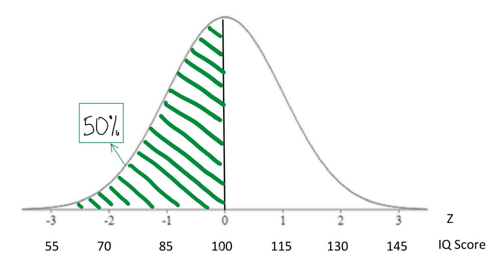
We saw that percentiles are expressions of area under a normal curve. Areas under the curve can be expressed as probability , too. For example, if we say the 50th percentile for IQ is 100, that can be expressed as: “If I chose a person at random, there is a 50% chance that they will have an IQ score below 100.”

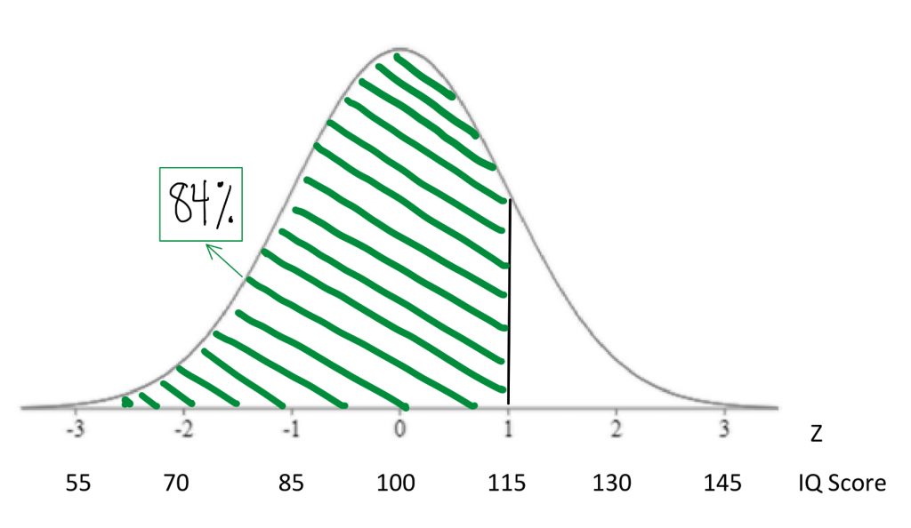
If we find the 84th percentile for IQ is 115 there is another way to say that “If I chose a person at random, there is an 84% chance that they will have an IQ score below 115.”

Concept Practice: find percentiles

Any time you are dealing with area under the normal curve, I encourage you to express that percentage in terms of probabilities . That will help you think clearly about what that area under the curve means once we get into the exercise of making decisions based on that information.

Concept Practice: interpreting percentile as probability

Probabilities , of course, range from 0 to 1 as proportions or fractions, and from 0% to 100% when expressed in percentage terms. In inferential statistics, we often express in terms of probability the likelihood that we would observe a particular score under a given normal curve model.

Concept Practice: applying probability

Although I encourage you to think of probabilities as percentages, the convention in statistics is to report to the probability of a score as a proportion, or decimal. The symbol used for “probability of score” is p . In statistics, the interpretation of “ p ” is a delicate subject. Generations of researchers have been lazy in our understanding of what “ p ”: tells us, and we have tended to over-interpret this statistic. As we begin to work with “ p ”, I will ask you to memorize a mantra that will help you report its meaning accurately. For now, just keep in mind that most psychologists and psychology students still make mistakes in how they express and understand the meaning of “ p ” values. This will take time and effort to fix, but I am confident that your generation will learn to do better at a precise and careful understanding of what statistics like “ p ” tell us… and what they do not.

To give you a sense of what a statement of p < .05 might mean, let us think back to our rat weights example.

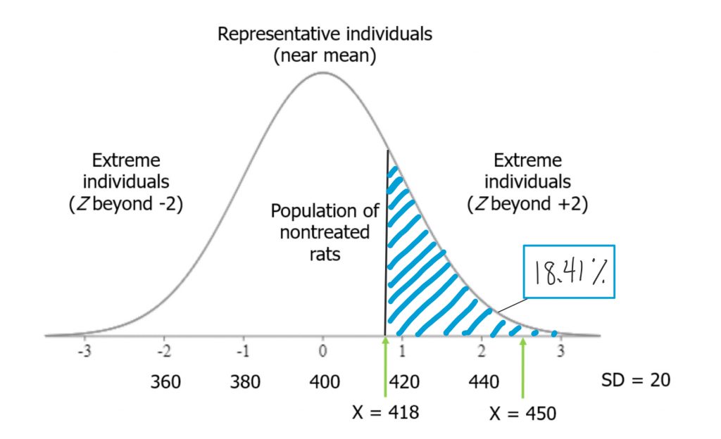
If I were to take a rat from our high-grain food group and place it on the distribution of untreated rat weights, and if it placed at Z = .9, we could look at the area under the curve from that point and above. That would tell us how likely it would be to observe such a heavy rat in the general population of nontreated rats — those that eat a normal diet.

Think of it this way. When we select a rat from our treatment group (those that ate the grain-heavy diet), and it is heavier than the average for a nontreated rat, there are two possible explanations for that observation. One is that the diet made him that way. As a scientist whose hypothesis is that a grain-heavy diet will make the rats weigh more, I’m actually motivated to interpret the observation that way. I want to believe this event is meaningful, because it is consistent with my hypothesis! But the other possibility is that, by random chance, we picked a rat that was heavy to begin with. There are plenty of rats in the distribution of nontreated rats that were at least that heavy. So there is always some probability that we just randomly selected a heavier rat. In this case, if my treated rat’s weight was less than one standard deviation above the mean, we saw in the chapter on normal curves that the probability of observing a rat weight that high or higher in the nontreated population was about 18%. That is not so unusual. It would not be terribly surprising if that outcome were simply the result of random chance rather than a result of the diet the rat had been eating.

If, on the other hand, the rat we measured was 2.5 standard deviations above the mean, the tail probability beyond that Z-score would be vanishingly small.

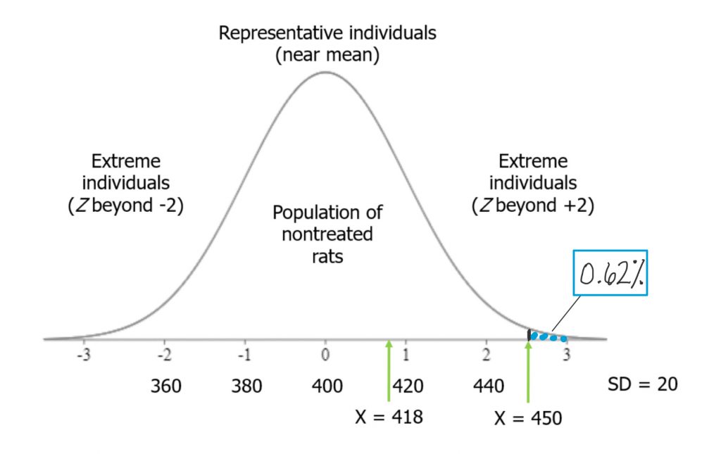
The probability of observing such a rat weight in the nontreated population is very low, so it is far less likely that observation can be accounted for just by random chance alone. As we accumulate more evidence, the probability they could have come at random from the nontreated population will weigh into our decision making about whether the grain-heavy diet indeed causes rats to become heavier. This is the way probabilities are used in the process of hypothesis testing , the logic of inferential statistics that we will look at soon.

Concept Practice: statistics as probability

Now that you have seen the relevance of probability to the decision making process that comprises inferential statistics, we have one more major learning objective: to become familiar with the central limit theorem .

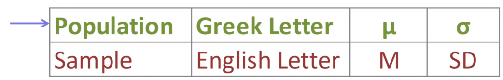
However, before we get to the central limit theorem , we need to be clear on the distinction between two concepts:  sample and population . In the world of statistics, the population is defined as all possible individuals or scores about which we would ideally draw conclusions. When we refer to the characteristics, or parameters, that describe a population , we will use Greek letters. A sample is defined as the individuals or scores about which we are actually drawing conclusions. When we refer to the characteristics, or statistics, that describe a sample , we will use English letters.

It is important to understand the difference between a population and a sample , and how they relate to one another, in order to comprehend the central limit theorem and its usefulness for statistics. From a population we can draw multiple samples . The larger sample , the more closely our sample will represent the population .

Think of a Venn diagram.  There is a circle that is a population . Inside that large circle, you can draw an infinite number of smaller circles, each of which represents a sample .

The larger that inner circle, the more of the population it contains, and thus the more representative it is.

Let us take a concrete example. A population might be the depression screening scores for all current postsecondary students in Canada. A sample from that population might be depression screening scores for 500 randomly selected postsecondary students from several institutions across Canada. That seems a more reasonable proportion of the two million students in the population than a sample that contains only 5 students. The 500 student sample has a better shot at adequately representing the entire population than does the 5 student sample , right? You can see that intuitively… and once you learn the central limit theorem , you will see the mathematical demonstration of the importance of sample size for representing the population .

To conduct the inferential statistics we are using in this course, we will be using the normal curve model to estimate probabilities associated with particular scores. To do that, we need to assume that data are normally distributed. However, in real life, our data are almost never actually a perfect match for the normal curve.

So how can we reasonably make the normality assumption? Here’s the thing. The central limit theorem is a mathematical principle that assures us that the normality assumption is a reasonable one as long as we have a decent sample size.

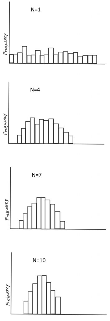
According to the theorem, as long as we take a decent-sized sample , if we took many samples (10,000) of large enough size (30+) and took the mean each time, the distribution of those means w ill approach a normal distribution, even if the scores from each sample are not normally distributed. To see this for yourself, take a look at the histograms shown on the right. The top histogram came from taking from a population 10,000 samples of just one score each, and plotting them on a histogram. See how it has a flat, or rectangular shape? No way we could call that a shape approximating a normal  curve. Next is a histogram that came from taking the means of 10,000 samples , if each sample included 4 scores. Looks slightly better, but still not very convincing. With a sample size of 7, it looks a bit better. Once our sample size is 10, we at least have something pretty close. Mathematically speaking, as long as the sample size is no smaller than 30, then the assumption of normality holds. The other way we can reasonably make the normality assumption is if we know the population itself follows a normal curve. In that case, even if individual samples do not have a nice shaped histogram, that is okay, because the normality assumption is one apply to the population in question, not to the sample itself.

Now, you can play around with an online demonstration so you can really convince yourself that the central limit theorem works in practice. The goal here is to see what sample size is sufficient to generate a histogram that closely approximates a normal curve. And to trust that even if real-life data look wonky, the normal curve may still be a reasonable model for data analysis for purposes of inference.

Concept Practice: Central Limit Theorem

4b. hypothesis testing.

We are finally ready for your first introduction to a formal decision making procedure often used in statistics, known as hypothesis testing .

In this course, we started off with descriptive statistics, so that you would become familiar with ways to summarize the important characteristics of datasets. Then we explored the concepts standardizing scores, and relating those to probability as area under the normal curve model. With all those tools, we are now ready to make something!

Okay, not furniture, exactly, but decisions.

We are now into the portion of the course that deals with inferential statistics. Just to get you thinking in terms of making decisions on the basis of data, let us take a slightly silly example. Suppose I have discovered a pill that cures hangovers!

Well, it greatly lessened symptoms of hangover in 10 of the 15 people I tested it on. I am charging 50 dollars per pill. Will you buy it the next time you go out for a night of drinking? Or recommend it to a friend? … If you said yes, I wonder if you are thinking very critically? Should we think about the cost-benefit ratio here on the basis of what information you have? If you said no, I bet some of the doubts I bring up popped to your mind as well. If 10 out of 15 people saw lessened symptoms, that’s 2/3 of people – so some people saw no benefits. Also, what does “greatly lessened symptoms of hangover” mean? Which symptoms? How much is greatly? Was the reduction by two or more standard deviations from the mean? Or was it less than one standard deviation improvement? Given the cost of 50 dollars per pill, I have to say I would be skeptical about buying it without seeing some statistics!

On this list is a preview of the basic concepts to which you will be introduced as we go through the rest of this chapter.

Hypothesis Testing Basic Concepts

• Null Hypothesis
• Research Hypothesis (alternative hypothesis)
• Statistical significance
• Conventional levels of significance
• Cutoff sample score (critical value)
• Directional vs. non-directional hypotheses
• One-tailed and two-tailed tests
• Type I and Type II errors

You can see that there are lots of new concepts to master. In my experience, each concept makes the most sense in context, within its place in the hypothesis testing workflow. We will start with defining our null and research hypotheses , then discuss the levels of statistical significance and their conventional usage. Next, we will look at how to find the cutoff sample score that will form the critical value for our decision criterion. We will look at how that differs for directional vs. non-directional hypotheses , which will lend themselves to one- or two-tailed tests , respectively.

The hypothesis testing procedure, or workflow, can be broken down into five discrete steps.

Steps of Hypothesis Testing

• Restate question as a research hypothesis and a null hypothesis about populations.
• Determine characteristics of the comparison distribution.
• Determine the cutoff sample score on the comparison distribution at which the null hypothesis should be rejected.
• Determine your sample’s score on the comparison distribution.
• Decide whether to reject the null hypothesis.

These steps are something we will be using pretty much the rest of the semester, so it is worth memorizing them now. My favourite approach to that is to create a mnemonic device. I recommend the following key words from which to form your mnemonic device: hypothesis, characteristics, cutoff, score, and decide. Not very memorable? Try association those with more memorable words that start with the same letter or sound. How about “ Happy Chickens Cure Sad Days .” Or you can put the words into a mnemonic device generator on the internet and get something truly bizarre. I just tried one and got “ Hairless Carsick Chewbacca Slapped Demons ”. Another good one: “ Hamlet Chose Cranky Sushi Drunkenly .” Anyway, you play around with it or brainstorm until you hit upon one that works for you. Who knew statistics could be this much fun!

The first step in hypothesis testing is always to formulate hypotheses. The first rule that will help you do so correctly, is that hypotheses are always about populations . We study samples in order to make conclusions about populations, so our predictions should be about the populations themselves. First, we define population 1 and population 2. Population 1 is always defined as people like the ones in our research study, the ones we are truly interested in. Population 2 is the comparison population , the status quo to which we are looking to compare our research population . Now, remember, when referring to populations , we always use Greek letters. So if we formulate our hypotheses in symbols, we need to use Greek letters.

It is a good idea to state our hypotheses both in symbols and in words. We need to make them specific and disprovable. If you follow my tips, you will have it down with just a little practice.

We need to state two hypotheses. First, we state the research hypothesis , which is sometimes referred to as the alternative hypothesis. The research hypothesis (often called the alternative hypothesis) is a statement of inequality, or that Something happened! This hypothesis makes the prediction that the population from which the research sample came is different from the comparison population . In other words, there is a really high probability that the sample comes from a different distribution than the comparison one.

The null hypothesis , on the other hand, is a statement of equality, or that nothing happened. This hypothesis makes the prediction that the population from which sample came is not different from the comparison population . We set up the null hypothesis as a so-called straw man, that we hope to tear down. Just remember, null means nothing – that nothing is different between the populations .

Step two of hypothesis testing is to determine the characteristics of the comparison distribution. This is where our descriptive statistics, the mean and standard deviation, come in. We need to ensure our normal curve model to which we are comparing our research sample is mapped out according to the particular characteristics of the population of comparison, which is population 2.

Next it is time to set our decision rule. Step 3 is to determine the cutoff sample score , which is derived from two pieces of information. The first is the conventional significance level that applies. By convention, the probability level that we are willing to accept as a risk that the score from our research sample might occur by random chance within the comparison distribution is set to one of three levels: 10%, 5%, or 1%. The most common choice of significance level is 5%. Typically the significance level will be provided to you in the problem for your statistics courses, but if it is not, just default to a significance level of .05. Sometimes researchers will choose a more conservative significance level , like 1%, if they are particularly risk averse. If the researcher chooses a 10% significance level , they are likely conducting a more exploratory study, perhaps a pilot study, and are not too worried about the probability that the score might be fairly common under the comparison distribution.

The second piece of information we need to know in order to find our cutoff sample score is which tail we are looking at. Is this a directional hypothesis , and thus one-tailed test ? Or a non-directional hypothesis , and thus a two-tailed test ? This depends on the research hypothesis from step 1. Look for directional keywords in the problem. If the researcher prediction involves words like “greater than” or “larger than”, this signals that we should be doing a one-tailed test and that our cutoff sample score should be in the top tail of the distribution. If the researcher prediction involves words like “lower than” or “smaller than”, this signals that we should be doing a one-tailed test and that our cutoff sample score should be in the bottom tail of the distribution. If the prediction is neutral in directionality, and uses a word like “different”, that signals a non-directional hypothesis . In that case, we would need to use a two-tailed test, and our cutoff scores would need to be indicated on both tails of the distribution. To do that, we take our area under the curve, which matches our significance level , and split it into both tails.

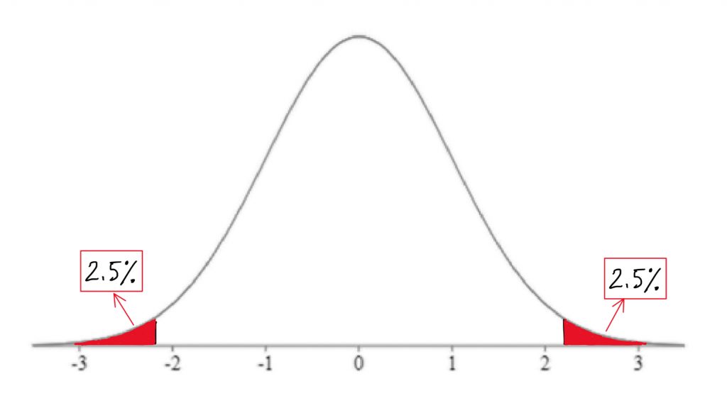
For example, if we have a two-tailed test with a .05 significance level , then we would split the 5% area under the curve into the two tails, so two and a half percent in each tail.

Concept Practice: deciding on one-tailed vs. two-tailed tests

We can find the Z-score that forms the border of the tail area we have identified based on significance level and directionality by looking it up in a table or an online calculator . I always recommend mapping this cutoff score onto a drawing of the comparison distribution as shown above. This should help you visualize the setup of the hypothesis test clearly and accurately.

Concept Practice: inference through hypothesis testing

The next step in the hypothesis testing procedure is to determine your sample’s score on the comparison distribution. To do this, we calculate a test statistic from the sample raw score, mark it on the comparison distribution, and determine whether it falls in the shaded tail or not. In reality, we would always have a sample with more than one score in it. However, for the sake of keeping our test statistic formula a familiar one, we will use a sample size of one. We will use our Z-score formula to translate the sample’s raw score into a Z-score – in other words, we will figure out how many standard deviations above or below the comparison distribution’s mean the sample score is.

Finally, it’s time to decide whether to reject the null hypothesis . This decision is based on whether our sample’s data point was more extreme than the cutoff score , in other words, “did it fall in the shaded tail?” If the sample score is more extreme than the cutoff score , then we must reject the null hypothesis. Our research hypothesis is supported! (Not proven… remember, there is still some probability that that score could have occurred randomly within the comparison distribution.) But it is sound to say that it appears quite likely that the population from which our sample came is different from the comparison population. Another way to express this decision is to say that the result was statistically significant , which is to say that there is less than a 5% chance of this result occurring randomly within the comparison distribution (here I just filled in the blank with the significance level).

What if the research sample score did not fall in the shaded tail? In the case that the sample score is less extreme than the cutoff score , then our research hypothesis is not supported. We do not reject the null hypothesis . It appears that the population from which our sample came is not different from the comparison population . Note that we do not typically express this result as “accept the null hypothesis” or “we have proved the null hypothesis”. From this test, we do not have evidence that the null hypothesis is correct, rather we simply did not have enough evidence to reject it. Another way to express this decision is to say that the result was not statistically significant , which is to say that there is more than a 5% chance of this result occurring randomly within the comparison distribution (here I just used the most common significance level ).

Concept Practice: interpreting conclusions of hypothesis tests

So we have described the hypothesis testing process from beginning to end. The whole process of null hypothesis testing can feel like pretty tortured logic at first. So let us zoom out, and look at the whole process another way. Essentially what we are seeking to do in such a hypothesis test is to compare two populations . We want to find out if the populations are distinct enough to confidently state that there is a difference between population 1 and population 2. In our example, we wanted to know if the population of people using a new medication, population 1, sleep longer than the population of people who are not using that new medication, population 2. We ended up finding that the research evidence to hand suggests population 1’s distribution is distinct enough from population 2 that we could reject the null hypothesis of similarity.

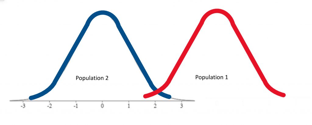
In other words, we were able to conclude that the difference between the centres of the two distributions was statistically significant .

If, on the other hand, the distributions were a bit less distinct, we would not have been able to make that claim of a significant difference.

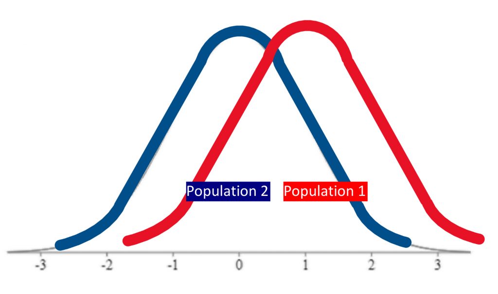
We would not have rejected the null hypothesis if evidence indicated the populations were too similar.

Just how different do the two distributions need to be? That criterion is set by the cutoff score , which depends on the significance level , and whether it is a one-tailed or two-tailed hypothesis test .

Concept Practice: Putting hypothesis test elements together

That was a lot of new concepts to take on! As a reward, assuming you enjoy memes, there are a plethora of statistics memes , some of which you may find funny now that you have made it into inferential statistics territory. Welcome to the exclusive club of people who have this rather peculiar sense of humour. Enjoy!

Chapter Summary

In this chapter we examined probability and how it can be used to make inferences about data in the framework of hypothesis testing . We now have a sense of how two populations can be compared and the difference between their means evaluated for statistical significance .

Concept Practice

Return to text.

Return to 4a. Probability and Inferential Statistics

Try interactive Worksheet 4a or download Worksheet 4a

Return to 4b. Hypothesis Testing

Try interactive Worksheet 4b  or download Worksheet 4b

in a situation where several different outcomes are possible, the probability of any specific outcome is a fraction or proportion of all possible outcomes

mathematical theorem that proposes the following: as long as we take a decent-sized sample, if we took many samples (10,000) of large enough size (30+) and took the mean each time, the distribution of those means will approach a normal distribution, even if the scores from each sample are not normally distributed

all possible individuals or scores about which we would ideally draw conclusions

a formal decision making procedure often used in inferential statistics

the individuals or scores about which we are actually drawing conclusions

the probability level that we are willing to accept as a risk that the score from our research sample might occur by random chance within the comparison distribution. By convention, it is set to one of three levels: 10%, 5%, or 1%.

critical value that serves as a decision criterion in hypothesis testing

prediction that the population from which the research sample came is different from the comparison population

the prediction that the population from which sample came is not different from the comparison population

a research prediction that the research population mean will be “greater than” or "less than" the comparison population mean

a hypothesis test in which there is only one cutoff sample score on either the lower or the upper end of the comparison distribution

a research prediction that the research population mean will be “different from" the comparison population mean, but allows for the possibility that the research population mean may be either greater than or less than the comparison population mean

a hypothesis test in which there are two cutoff sample scores, one on either end of the comparison distribution

a decision in hypothesis testing that concludes statistical significance because the sample score is more extreme than the cutoff score

the conclusion from a hypothesis test that probability of the observed result occurring randomly within the comparison distribution is less than the significance level

a decision in hypothesis testing that is inconclusive because the sample score is less extreme than the cutoff score

Beginner Statistics for Psychology Copyright © 2021 by Nicole Vittoz is licensed under a Creative Commons Attribution-NonCommercial 4.0 International License , except where otherwise noted.

Have a thesis expert improve your writing

Check your thesis for plagiarism in 10 minutes, generate your apa citations for free.

• Knowledge Base
• Inferential Statistics | An Easy Introduction & Examples

Inferential Statistics | An Easy Introduction & Examples

Published on 18 January 2023 by Pritha Bhandari .

While descriptive statistics summarise the characteristics of a data set, inferential statistics help you come to conclusions and make predictions based on your data.

When you have collected data from a sample , you can use inferential statistics to understand the larger population from which the sample is taken.

Inferential statistics have two main uses:

• making estimates about populations (for example, the mean SAT score of all 11th graders in the US).
• testing hypotheses to draw conclusions about populations (for example, the relationship between SAT scores and family income).

Table of contents

Descriptive versus inferential statistics, estimating population parameters from sample statistics, hypothesis testing, frequently asked questions.

Descriptive statistics allow you to describe a data set, while inferential statistics allow you to make inferences based on a data set.

Descriptive statistics

Using descriptive statistics, you can report characteristics of your data:

• The distribution concerns the frequency of each value.
• The central tendency concerns the averages of the values.
• The variability concerns how spread out the values are.

In descriptive statistics, there is no uncertainty – the statistics precisely describe the data that you collected. If you collect data from an entire population, you can directly compare these descriptive statistics to those from other populations.

Inferential statistics

Most of the time, you can only acquire data from samples, because it is too difficult or expensive to collect data from the whole population that you’re interested in.

While descriptive statistics can only summarise a sample’s characteristics, inferential statistics use your sample to make reasonable guesses about the larger population.

With inferential statistics, it’s important to use random and unbiased sampling methods . If your sample isn’t representative of your population, then you can’t make valid statistical inferences or generalise .

Sampling error in inferential statistics

Since the size of a sample is always smaller than the size of the population, some of the population isn’t captured by sample data. This creates sampling error , which is the difference between the true population values (called parameters) and the measured sample values (called statistics).

Sampling error arises any time you use a sample, even if your sample is random and unbiased. For this reason, there is always some uncertainty in inferential statistics. However, using probability sampling methods reduces this uncertainty.

The characteristics of samples and populations are described by numbers called statistics and parameters :

• A statistic is a measure that describes the sample (e.g., sample mean ).
• A parameter is a measure that describes the whole population (e.g., population mean).

Sampling error is the difference between a parameter and a corresponding statistic. Since in most cases you don’t know the real population parameter, you can use inferential statistics to estimate these parameters in a way that takes sampling error into account.

There are two important types of estimates you can make about the population: point estimates and interval estimates .

• A point estimate is a single value estimate of a parameter. For instance, a sample mean is a point estimate of a population mean.
• An interval estimate gives you a range of values where the parameter is expected to lie. A confidence interval is the most common type of interval estimate.

Both types of estimates are important for gathering a clear idea of where a parameter is likely to lie.

Confidence intervals

A confidence interval uses the variability around a statistic to come up with an interval estimate for a parameter. Confidence intervals are useful for estimating parameters because they take sampling error into account.

While a point estimate gives you a precise value for the parameter you are interested in, a confidence interval tells you the uncertainty of the point estimate. They are best used in combination with each other.

Each confidence interval is associated with a confidence level. A confidence level tells you the probability (in percentage) of the interval containing the parameter estimate if you repeat the study again.

A 95% confidence interval means that if you repeat your study with a new sample in exactly the same way 100 times, you can expect your estimate to lie within the specified range of values 95 times.

Although you can say that your estimate will lie within the interval a certain percentage of the time, you cannot say for sure that the actual population parameter will. That’s because you can’t know the true value of the population parameter without collecting data from the full population.

However, with random sampling and a suitable sample size, you can reasonably expect your confidence interval to contain the parameter a certain percentage of the time.

Your point estimate of the population mean paid vacation days is the sample mean of 19 paid vacation days.

Hypothesis testing is a formal process of statistical analysis using inferential statistics. The goal of hypothesis testing is to compare populations or assess relationships between variables using samples.

Hypotheses , or predictions, are tested using statistical tests . Statistical tests also estimate sampling errors so that valid inferences can be made.

Statistical tests can be parametric or non-parametric. Parametric tests are considered more statistically powerful because they are more likely to detect an effect if one exists.

Parametric tests make assumptions that include the following:

• the population that the sample comes from follows a normal distribution of scores
• the sample size is large enough to represent the population
• the variances , a measure of variability , of each group being compared are similar

When your data violates any of these assumptions, non-parametric tests are more suitable. Non-parametric tests are called ‘distribution-free tests’ because they don’t assume anything about the distribution of the population data.

Statistical tests come in three forms: tests of comparison, correlation or regression.

Comparison tests

Comparison tests assess whether there are differences in means, medians or rankings of scores of two or more groups.

To decide which test suits your aim, consider whether your data meets the conditions necessary for parametric tests, the number of samples, and the levels of measurement of your variables.

Means can only be found for interval or ratio data , while medians and rankings are more appropriate measures for ordinal data .

Correlation tests

Correlation tests determine the extent to which two variables are associated.

Although Pearson’s r is the most statistically powerful test, Spearman’s r is appropriate for interval and ratio variables when the data doesn’t follow a normal distribution.

The chi square test of independence is the only test that can be used with nominal variables.

Regression tests

Regression tests demonstrate whether changes in predictor variables cause changes in an outcome variable. You can decide which regression test to use based on the number and types of variables you have as predictors and outcomes.

Most of the commonly used regression tests are parametric. If your data is not normally distributed, you can perform data transformations.

Data transformations help you make your data normally distributed using mathematical operations, like taking the square root of each value.

Descriptive statistics summarise the characteristics of a data set. Inferential statistics allow you to test a hypothesis or assess whether your data is generalisable to the broader population.

A statistic refers to measures about the sample , while a parameter refers to measures about the population .

A sampling error is the difference between a population parameter and a sample statistic .

Hypothesis testing is a formal procedure for investigating our ideas about the world using statistics. It is used by scientists to test specific predictions, called hypotheses , by calculating how likely it is that a pattern or relationship between variables could have arisen by chance.

Cite this Scribbr article

If you want to cite this source, you can copy and paste the citation or click the ‘Cite this Scribbr article’ button to automatically add the citation to our free Reference Generator.

Bhandari, P. (2023, January 18). Inferential Statistics | An Easy Introduction & Examples. Scribbr. Retrieved 3 June 2024, from https://www.scribbr.co.uk/stats/inferential-statistics-meaning/

Is this article helpful?

Pritha Bhandari

Other students also liked, descriptive statistics | definitions, types, examples, understanding confidence intervals | easy examples & formulas, how to calculate variance | calculator, analysis & examples.

Research Methods in Psychology

14. inferential statistics ¶.

The great tragedy of science - the slaying of a beautiful hypothesis by an ugly fact. —Thomas Huxley

Truth in science can be defined as the working hypothesis best suited to open the way to the next better one. —Konrad Lorenz

Recall that Matthias Mehl and his colleagues, in their study of sex differences in talkativeness, found that the women in their sample spoke a mean of 16,215 words per day and the men a mean of 15,669 words per day [MVRamirezE+07] . But despite observing this difference in their sample, they concluded that there was no evidence of a sex difference in talkativeness in the population. Recall also that Allen Kanner and his colleagues, in their study of the relationship between daily hassles and symptoms, found a correlation of 0.6 in their sample [KCSL81] . But they concluded that this finding implied a relationship between hassles and symptoms in the population. These examples raise questions about how researchers can draw conclusions about the population based on results from their sample.

To answer such questions, researchers use a set of techniques called inferential statistics, which is what this chapter is about. We focus, in particular, on null hypothesis testing, the most common approach to inferential statistics in psychological research. We begin with a conceptual overview of null hypothesis testing, including its purpose and basic logic. Then we look at several null hypothesis testing techniques that allow conclusions about differences between means and about correlations between quantitative variables. Finally, we consider a few other important ideas related to null hypothesis testing, including some that can be helpful in planning new studies and interpreting results. We also look at some long-standing criticisms of null hypothesis testing and some ways of dealing with these criticisms.

14.1. Understanding Null Hypothesis Testing ¶

14.1.1. learning objectives ¶.

Explain the purpose of null hypothesis testing, including the role of sampling error.

Describe the basic logic of null hypothesis testing.

Describe the role of relationship strength and sample size in determining statistical significance and make reasonable judgments about statistical significance based on these two factors.

14.1.2. The Purpose of Null Hypothesis Testing ¶

As we have seen, psychological research typically involves measuring one or more variables within a sample and computing descriptive statistics. In general, however, the researcher’s goal is not to draw conclusions about the participants in that sample, but rather to draw conclusions about the population from which those participants were selected. Thus, researchers must use sample statistics to draw conclusions about the corresponding values in the population. These corresponding values in the population are called parameters. Imagine, for example, that a researcher measures the number of depressive symptoms exhibited by each of 50 clinically depressed adults and computes the mean number of symptoms. The researcher probably wants to use this sample statistic (the mean number of symptoms for the sample) to draw conclusions about the corresponding population parameter (the mean number of symptoms for clinically depressed adults).

Unfortunately, sample statistics are not perfect estimates of their corresponding population parameters. This is because there is a certain amount of random variability in any statistic from sample to sample. The mean number of depressive symptoms might be 8.73 in one sample of clinically depressed adults, 6.45 in a second sample, and 9.44 in a third. This will happen even though these samples are randomly selected from the same population. Similarly, the correlation (e.g., Pearson’s r) between two variables might be 0.24 in one sample, -0.04 in a second sample, and 0.15 in a third. Again, this can and will happen even though these samples are selected randomly from the same population. This random variability in statistics calculated from sample to sample is called sampling error. Note that the term error here refers to the statistical notion of error, or random variability, and does not imply that anyone has made a mistake. No one “commits a sampling error”.

One implication of this is that when there is a statistical relationship in a sample, it is not always clear whether there is a statistical relationship in the population. A small difference between two group means in a sample might indicate that there is a small difference between the two group means in the population. But it could also be that there is no difference between the means in the population and that the difference in the sample is just a matter of sampling error. Similarly, a Pearson’s r value of -0.29 in a sample might mean that there is a negative relationship in the population. But it could also be that there is no relationship in the population and that the relationship in the sample is just a matter of sampling error.

In fact, any relationship observed in a sample can be interpreted in two ways:

There is a relationship in the population, and the relationship in the sample reflects this.

There is no relationship in the population, and the relationship in the sample reflects only sampling error.

The purpose of inferential statistics is simply to help researchers decide between these two interpretations.

14.1.3. The Logic of Null Hypothesis Testing ¶

Null hypothesis testing (or NHST) is a formal approach to making decisions between these two interpretations. One interpretation is called the null hypothesis (often symbolized \(H_0\) and read as “H-naught”). This is the idea that there is no relationship in the population and that the relationship in the sample reflects only sampling error. Informally, the null hypothesis is that the sample relationship “occurred by chance”. The other interpretation is called the alternative hypothesis (often symbolized as \(H_1\) ). This is the idea that there is a relationship in the population and that the relationship in the sample reflects this relationship in the population.

Again, every statistical relationship in a sample can be interpreted in either of these two ways: It might have occurred by chance, or it might reflect a relationship in the population. So researchers need a way to decide between them. Although there are many specific null hypothesis testing techniques, they are all based on the same general logic. The steps are as follows:

Assume for the moment that the null hypothesis is true. There is no relationship between the variables in the population.

Determine how likely the sample relationship would be if the null hypothesis were true.

If the sample relationship would be extremely unlikely, then reject the null hypothesis in favor of the alternative hypothesis. If it would not be extremely unlikely, then retain the null hypothesis.

Following this logic, we can begin to understand why Mehl and his colleagues concluded that there is no difference in talkativeness between women and men in the population. In essence, they asked the following question: “If there were no difference in the population, how likely is it that we would find a small difference of d = 0.06 in our sample?” Their answer to this question was that this sample relationship would be fairly likely if the null hypothesis were true. Therefore, they retained the null hypothesis—concluding that there is no evidence of a sex difference in the population. We can also see why Kanner and his colleagues concluded that there is a correlation between hassles and symptoms in the population. They asked, “If the null hypothesis were true, how likely is it that we would find a strong correlation of +.60 in our sample?” Their answer to this question was that this sample relationship would be fairly unlikely if the null hypothesis were true. Therefore, they rejected the null hypothesis in favor of the alternative hypothesis—concluding that there is a positive correlation between these variables in the population.

A crucial step in null hypothesis testing is finding the likelihood of the sample result if the null hypothesis were true. This probability is called the p value. A small value of p value means that the sample result would be unlikely if the null hypothesis were true and leads to the rejection of the null hypothesis. A large value of p means that the sample result would be likely if the null hypothesis were true and leads the null hypothesis to be accepted. But how low must the p value be before the sample result is considered unlikely enough to reject the null hypothesis? In null hypothesis testing, this criterion is called \(\alpha\) (alpha) and is often set to .05. If the chance of a result as extreme as the sample result (or more extreme) is less than a 5% if the null hypothesis were true, then the null hypothesis is rejected. When this happens, the result is said to be statistically significant. If the chance of of a result as extreme as the sample result is greater than 5% when the null hypothesis is true, then the null hypothesis is retained. This does not necessarily mean that the researcher accepts the null hypothesis as true. It means that there is not currently enough evidence to conclude that it is false. For this reason, researchers often use the expression “fail to reject the null hypothesis” rather than something such as “conclude the null hypothesis is true”.

14.1.4. The Misunderstood p Value ¶

The p value is one of the most misunderstood quantities in psychological research [Coh94] . Even professional researchers misinterpret it, and it is not unusual for such misinterpretations to appear in statistics textbooks!

The most common misinterpretation is that the p value is the probability that the null hypothesis is true or that the that the p value is the probability that the sample result occurred by chance. For example, a misguided researcher might say that because the p value is .02, there is only a 2% chance that the result is due to chance and a 98% chance that it reflects a real relationship in the population. But this is incorrect. The p value is really the probability of a result at least as extreme as the sample result if the null hypothesis were true. So a p value of .02 means that if the null hypothesis were true, a sample result this extreme would occur only 2% of the time.

You can avoid this misunderstanding by remembering that the p value is not the probability that any particular hypothesis is true or false. Instead, it is the probability of obtaining the sample result if the null hypothesis were true.

14.1.5. Role of Sample Size and Relationship Strength ¶

Recall that null hypothesis testing involves answering the question, “If the null hypothesis were true, what is the probability of a sample result as extreme as this one?” As we have just seen, this question is equivalent to, “What is the p value?” It can be helpful to see that the answer to this question depends on just two considerations: the strength of the relationship and the size of the sample. Specifically, the stronger the sample relationship and the larger the sample, the less likely the result would be if the null hypothesis were true. That is, the lower the p value. This should make sense. Imagine a study in which a sample of 500 women is compared with a sample of 500 men in terms of some psychological characteristic, and Cohen’s d is a strong 0.50. If there were really no sex difference in the population, then a result this strong based on such a large sample should seem highly unlikely. Now imagine a similar study in which a sample of three women is compared with a sample of three men, and Cohen’s d is a weak 0.10. If there were no sex difference in the population, then a relationship this weak based on such a small sample should seem likely. And this is precisely why the null hypothesis would be rejected in the first example and retained in the second.

Of course, sometimes the result can be weak and the sample large, or the result can be strong and the sample small. In these cases, the two considerations trade off against each other so that a weak result can be statistically significant if the sample is large enough and a strong relationship can be statistically significant even if the sample is small. Figure 14.1: shows a rough guideline of how relationship strength and sample size might combine to determine whether a sample result is statistically significant or not. The columns of the table represent the three levels of relationship strength: weak, medium, and strong. The rows represent four sample sizes that can be considered small, medium, large, and extra large in the context of psychological research. Thus, each cell in the table represents a combination of relationship strength and sample size. If a cell contains the word Yes, then this combination would be statistically significant for both Cohen’s d and Pearson’s r. If it contains the word No, then it would not be statistically significant for either. There is one cell where the decision for d and r would be different and another where it might be different depending on some additional considerations, which are discussed below, in the section entitled, “Some Basic Null Hypothesis Tests”.

Fig. 14.1 How Relationship Strength and Sample Size Combine to Determine Whether a Result Is Statistically Significant ¶

Although Figure 14.1: provides only a rough guideline, it shows very clearly that weak relationships based on medium or small samples are less likely to be statistically significant and that strong relationships based on medium or larger samples are more likely to be statistically significant. If you keep this lesson in mind, you will often know whether a result is statistically significant based on the descriptive statistics alone. It is extremely useful to be able to develop this kind of intuitive judgment. One reason is that it allows you to develop expectations about how your formal null hypothesis tests are going to come out, which in turn allows you to detect problems in your analyses. For example, if your sample relationship is strong and your sample is medium, then you would expect to reject the null hypothesis. If for some reason your formal null hypothesis test indicates otherwise, then you may need to double-check your computations and interpretations. A second reason is that the ability to make this kind of intuitive judgment is an indication that you understand the basic logic of this approach.

14.1.6. Statistical Significance Versus Practical Significance ¶

Figure 14.1: illustrates another extremely important point. A statistically significant result is not necessarily a strong one. Even a very weak result can be statistically significant if it is based on a large enough sample. This is closely related to Janet Shibley Hyde’s argument about sex differences [Hyd07] . The differences between women and men in mathematical problem solving and leadership ability are statistically significant. But the word “significant” can cause people to interpret these differences as strong and important, perhaps even important enough to influence the college courses they take or even who they vote for. As we have seen, however, these statistically significant differences are actually quite weak, perhaps even “trivial”.

This is why it is important to distinguish between the statistical significance of a result and the practical significance of that result. Practical significance refers to the importance or usefulness of the result in some real-world context. Many sex differences are statistically significant (and may even be interesting for purely scientific reasons) but they are often not practically significant. In clinical practice, this same concept is often referred to as “clinical significance”. For example, a study on a new treatment for social phobia might show that it produces a positive effect that is statistically significant. Yet this effect still might not be strong enough to justify the time, effort, and other costs of putting it into practice. For example, easier and cheaper treatments that work almost as well might already exist. Although statistically significant, this result would be said to lack practical or clinical significance.

14.1.7. Key Takeaways ¶

Null hypothesis testing is a formal approach to deciding whether a statistical relationship in a sample reflects a real relationship in the population or is just due to chance.

The logic of null hypothesis testing involves assuming that the null hypothesis is true, finding how likely the sample result would be if this assumption were correct, and then making a decision. If the sample result would be unlikely if the null hypothesis were true, then it is rejected in favor of the alternative hypothesis. If it would not be unlikely, then the null hypothesis is retained.

The probability of obtaining the sample result if the null hypothesis were true (the p value) is based on two considerations: relationship strength and sample size. Reasonable judgments about whether a sample relationship is statistically significant can often be made by quickly considering these two factors.

Statistical significance is not the same as relationship strength or importance. Even weak relationships can be statistically significant if the sample size is large enough. It is important to consider relationship strength and the practical significance of a result in addition to its statistical significance.

14.1.8. Exercises ¶

Discussion: Imagine a study showing that people who eat more broccoli tend to be happier. Explain for someone who knows nothing about statistics why the researchers would conduct a null hypothesis test.

Practice: Use Figure 14.1: to try and determine whether each of the following results is statistically significant:

a. The correlation between two variables is r = -0.78 based on a sample size of 137.

b. The mean score on a psychological characteristic for women is 25 (SD = 5) and the mean score for men is 24 (SD = 5). There were 12 women and 10 men in this study.

c. In a memory experiment, the mean number of items recalled by the 40 participants in Condition A was 0.50 standard deviations greater than the mean number recalled by the 40 participants in Condition B.

d. In another memory experiment, the mean scores for participants in Condition A and Condition B came out exactly the same!

e. A student finds a correlation of r = 0.04 between the number of units the students in his research methods class are taking and the students’ level of stress.

14.2. Some Basic Null Hypothesis Tests ¶

14.2.1. learning objectives ¶.

Conduct and interpret one-sample, dependent-samples, and independent-samples t tests.

Interpret the results of one-way, repeated measures, and factorial ANOVAs.

Conduct and interpret null hypothesis tests of Pearson’s r.

In this section, we look at several common null hypothesis testing procedures. The emphasis here is on providing enough information to allow you to conduct and interpret the most basic versions. In most cases, the online statistical analysis tools mentioned in Chapter 13 will handle the computations, as will programs such as Microsoft Excel and SPSS.

14.2.2. The t Test ¶

As we have seen throughout this book, many studies in psychology focus on the difference between two means. The most common null hypothesis test for this type of statistical relationship is the t test. In this section, we look at three types of t tests that are used for slightly different research designs: the one-sample t test, the dependent-samples t test, and the independent-samples t test.

14.2.3. One-Sample t Test ¶

The one-sample t test is used to compare a sample mean (M) with a hypothetical population mean ( \(\mu_0\) ) that provides some interesting standard of comparison. The null hypothesis is that the mean for the population ( \(\mu\) ) is equal to the hypothetical population mean: \(\mu\) = \(\mu_0\) . The alternative hypothesis is that the mean for the population is different from the hypothetical population mean: \(\mu \neq \mu_0\) . To decide between these two hypotheses, we need to find the probability of obtaining the sample mean (or one more extreme) if the null hypothesis were true. But finding this p value requires first computing a test statistic called t. A test statistic is a statistic that is computed only to help find the p value. The formula for t is as follows:

Again, M is the sample mean and \(\mu_0\) is the hypothetical population mean of interest. SD is the sample standard deviation and N is the sample size.

The reason the t statistic (or any test statistic) is useful is that we know how it is distributed when the null hypothesis is true. As shown in Figure 14.2: , this distribution is unimodal and symmetrical, and it has a mean of 0. Its precise shape depends on a statistical concept called the degrees of freedom, which for a one-sample t test is N - 1 (there are 24 degrees of freedom for the distribution shown in Figure 14.2: ). The important point is that knowing this distribution makes it possible to find the p value for any t score. Consider, for example, a t score of +1.50 based on a sample of 25. The probability of a t score at least this extreme is given by the proportion of t scores in the distribution that are at least this extreme. For now, let us define extreme as being far from zero in either direction. Thus the p value is the proportion of t scores that are +1.50 or above or that are -1.50 or below, a value that turns out to be .14.

Fig. 14.2 Distribution of t Scores (with 24 Degrees of Freedom) when the null hypothesis is true. The red vertical lines represent the two-tailed critical values, and the green vertical lines the one-tailed critical values when \(\alpha\) = .05. ¶

Fortunately, we do not have to deal directly with the distribution of t scores. If we were to enter our sample data and hypothetical mean of interest into one of the online statistical tools in Chapter 13 or into a program like SPSS, the output would include both the t score and the p value. At this point, the rest of the procedure is simple. If p is less than .05, we reject the null hypothesis and conclude that the population mean differs from the hypothetical mean of interest. If p is greater than .05, we conclude that there is not enough evidence to say that the population mean differs from the hypothetical mean of interest.

If we were to compute the t score by hand, we could use a table below to make the decision. This table does not provide actual p values. Instead, it provides the critical values of t for different degrees of freedom (df) when \(\alpha\) is .05. For now, let us focus on the two-tailed critical values in the last column of the table. Each of these values should be interpreted as a pair of values: one positive and one negative. For example, the two-tailed critical values when there are 24 degrees of freedom are +2.064 and -2.064. These are represented by the red vertical lines in Figure 14.2: . The idea is that any t score below the lower critical value (the left-hand red line in Figure Figure 14.2: ) is in the lowest 2.5% of the distribution, while any t score above the upper critical value (the right-hand red line) is in the highest 2.5% of the distribution. Therefore any t score beyond the critical value in either direction is in the most extreme 5% of t scores when the null hypothesis is true and has a p value less than .05. Thus if the t score we compute is beyond the critical value in either direction, then we reject the null hypothesis. If the t score we compute is between the upper and lower critical values, then we retain the null hypothesis.

Thus far, we have considered what is called a two-tailed test, where we reject the null hypothesis if the t score for the sample is extreme in either direction. This test makes sense when we believe that the sample mean might differ from the hypothetical population mean but we do not have good reason to expect the difference to go in a particular direction. But it is also possible to do a one-tailed test, where we reject the null hypothesis only if the t score for the sample is extreme in one direction that we specify before collecting the data. This test makes sense when we have good reason to expect the sample mean will differ from the hypothetical population mean in a particular direction.

Here is how it works. Each one-tailed critical value in the table above can again be interpreted as a pair of values: one positive and one negative. A t score below the lower critical value is in the lowest 5% of the distribution, and a t score above the upper critical value is in the highest 5% of the distribution. For 24 degrees of freedom, these values are -1.711 and +1.711 (these are represented by the green vertical lines in Figure 14.2: ). However, for a one-tailed test, we must decide before collecting data whether we expect the sample mean to be lower than the hypothetical population mean, in which case we would use only the lower critical value, or we expect the sample mean to be greater than the hypothetical population mean, in which case we would use only the upper critical value. Notice that we still reject the null hypothesis when the t score for our sample is in the most extreme 5% of the t scores we would expect if the null hypothesis were true, keeping \(\alpha\) at .05. We have simply redefined “extreme” to refer only to one tail of the distribution. The advantage of the one-tailed test is that critical values in that tail are less extreme. If the sample mean differs from the hypothetical population mean in the expected direction, then we have a better chance of rejecting the null hypothesis. The disadvantage is that if the sample mean differs from the hypothetical population mean in the unexpected direction, then there is no chance of rejecting the null hypothesis.

14.2.4. Example One-Sample t Test ¶

Imagine that a health psychologist is interested in the accuracy of university students’ estimates of the number of calories in a chocolate chip cookie. He shows the cookie to a sample of 10 students and asks each one to estimate the number of calories in it. Because the actual number of calories in the cookie is 250, this is the hypothetical population mean of interest ( \(\mu_0\) ). The null hypothesis is that the mean estimate for the population ( \(\mu\) ) is 250. Because he has no real sense of whether the students will underestimate or overestimate the number of calories, he decides to do a two-tailed test. Now imagine further that the participants’ actual estimates are as follows:

250, 280, 200, 150, 175, 200, 200, 220, 180, 250

The mean estimate for the sample (M) is 212.00 calories and the standard deviation (SD) is 39.17. The health psychologist can now compute the t score for his sample:

If he enters the data into one of the online analysis tools or uses SPSS, it would also tell him that the two- tailed p value for this t score (with 10 - 1 = 9 degrees of freedom) is .013. Because this is less than .05, the health psychologist would reject the null hypothesis and conclude that university students tend to underestimate the number of calories in a chocolate chip cookie. If he computes the t score by hand, he could look at Table 13.2 and see that the critical value of t for a two-tailed test with 9 degrees of freedom is ±2.262. The fact that his t score was more extreme than this critical value would tell him that his p value is less than .05 and that he should reject the null hypothesis.

Finally, if this researcher had gone into this study with good reason to expect that university students underestimate the number of calories, then he could have done a one-tailed test instead of a two-tailed test. The only thing this decision would change is the critical value, which would be -1.833. This slightly less extreme value would make it a bit easier to reject the null hypothesis. However, if it turned out that university students overestimate the number of calories the researcher would not have been able to reject the null hypothesis, no matter how much they overestimated it.

14.2.5. The Dependent-Samples t Test ¶

The dependent-samples t test (sometimes called the paired-samples t test) is used to compare two means (e.g., a group of participants measured at two different times or under two different conditions). This comparison is appropriate for pretest-posttest designs or within-subjects experiments. The null hypothesis is that the two means are the same in the population. The alternative hypothesis is that they are not the same. Like the one-sample t test, te dependent-samples t test can be one-tailed if the researcher has good reason to expect the difference goes in a particular direction.

It helps to think of the dependent-samples t test as a special case of the one-sample t test. However, the first step in the dependent-samples t test is to reduce the two scores for each participant to a single measurement by taking the difference between them. At this point, the dependent-samples t test becomes a one-sample t test on the difference scores. The hypothetical population mean ( \(\mu_0\) ) of interest is 0 because this is what the mean difference score would be if there were no difference between the two means. We can now think of the null hypothesis as being that the mean difference score in the population is 0 ( \(\mu_0\) = 0) and the alternative hypothesis as being that the mean difference score in the population is not 0 ( \(\mu_0 \neq 0\) ).

14.2.6. Example Dependent-Samples t Test ¶

Imagine that the health psychologist now knows that people tend to underestimate the number of calories in junk food and has developed a short training program to improve their estimates. To test the effectiveness of this program, he conducts a pretest-posttest study in which 10 participants estimate the number of calories in a chocolate chip cookie before the training program and then estimate the calories again afterward. Because he expects the program to increase participants’ estimates, he decides to conduct a one-tailed test. Now imagine further that the pretest estimates are:

230, 250, 280, 175, 150, 200, 180, 210, 220, 190

and that the posttest estimates (for the same participants in the same order) are:

250, 260, 250, 200, 160, 200, 200, 180, 230, 240.

The difference scores, then, are as follows:

+20, +10, -30, +25, +10, 0, +20, -30, +10, +50.

Note that it does not matter whether the first set of scores is subtracted from the second or the second from the first as long as it is done the same way for all participants. In this example, it makes sense to subtract the pretest estimates from the posttest estimates so that positive difference scores mean that the estimates went up after the training and negative difference scores mean the estimates went down.

The mean of the difference scores is 8.50 with a standard deviation of 27.27. The health psychologist can now compute the t score for his sample as follows:

If he enters the data into one of the online analysis tools or uses Excel or SPSS, it would tell him that the one-tailed p value for this t score (again with 10 - 1 = 9 degrees of freedom) is .148. Because this is greater than .05, he would fail to reject the null hypothesis; he does not have enough evidence to suggest that the training program increases calorie estimates. If he were to compute the t score by hand, he could look at the table above and see that the critical value of t for a one-tailed test with 9 degrees of freedom is +1.833 (positive because he was expecting a positive mean difference score). The fact that his t score was less extreme than this critical value would tell him that his p value is greater than .05 and that the results fail to reject the null hypothesis.

14.2.7. The Independent-Samples t Test ¶

The independent-samples t test is used to compare the means of two separate samples (M1 and M2). The two samples might have been tested under different conditions in a between-subjects experiment, or they could be preexisting groups in a correlational design (e.g., women and men or extraverts and introverts). The null hypothesis is that the two means: \(\mu_1 = \) \mu_2 \(. The alternative hypothesis is that they are not the same: \) \mu_1 \neq \mu_2$. Again, the test can be one-tailed if the researcher has good reason to expect the difference goes in a particular direction.

The t statistic here is a bit more complicated because it must take into account two sample means, two standard deviations, and two sample sizes. The formula is as follows:

Notice that this formula includes squared standard deviations (the variances) that appear inside the square root symbol. Also, lowercase n1 and n2 refer to the sample sizes in the two groups or condition (as opposed to capital N, which generally refers to the total sample size). The only additional thing to know here is that there are N - 2 degrees of freedom for the independent-samples t test.

14.2.8. Example Independent-Samples t test ¶

Now the health psychologist wants to compare the calorie estimates of people who regularly eat junk food with the estimates of people who rarely eat junk food. He believes the difference could come out in either direction so he decides to conduct a two-tailed test. He collects data from a sample of eight participants who eat junk food regularly and seven participants who rarely eat junk food. The data are as follows:

Junk food eaters: 180, 220, 150, 85, 200, 170, 150, 190

Non–junk food eaters: 200, 240, 190, 175, 200, 300, 240

The mean for the junk food eaters is 220.71 with a standard deviation of 41.23. The mean for the non–junk food eaters is 168.12 with a standard deviation of 42.66. He can now compute his t score as follows:

If he enters the data into one of the online analysis tools or uses Excel or SPSS, it would tell him that the two-tailed p value for this t score (with 15 - 2 = 13 degrees of freedom) is .015. Because this p value is less than .05, the health psychologist would reject the null hypothesis and conclude that people who eat junk food regularly make lower calorie estimates than people who eat it rarely. If he were to compute the t score by hand, he could look at the table above and see that the critical value of t for a two-tailed test with 13 degrees of freedom is 2.160 (and/or -2.160). The fact that the observed t score was more extreme than this critical value would tell him that his p value is less than .05 and that he should reject the null hypothesis.

14.2.9. The Analysis of Variance ¶

When there are more than two groups or condition means to be compared, the most common null hypothesis test is the analysis of variance (ANOVA). In this section, we look primarily at the one-way ANOVA, which is used for between-subjects designs with a single independent variable. We then briefly consider some other versions of the ANOVA that are used for within-subjects and factorial research designs.

14.2.10. One-Way ANOVA ¶

The one-way ANOVA is used to compare the means of more than two samples ( \(M_1, M_2, \ldots M_G\) ) in a between-subjects design. The null hypothesis is that all the means are equal in the population: \(\mu_1=\mu_2= \ldots = \mu_G\) . The alternative hypothesis is that not all the means in the population are equal.

The test statistic for the ANOVA is called F. It is a ratio of two estimates of the population variance based on the sample data. One estimate of the population variance is called the mean squares between groups (MSB) and is based on the differences among the sample means. The other is called the mean squares within groups (MSW) and is based on the differences among the scores within each group. The F statistic is the ratio of the \(MS_B\) to the \(MS_W\) and can therefore be expressed as follows:

Again, the reason that F is useful is that we know how it is distributed when the null hypothesis is true. As shown in Figure 14.3: , this distribution is unimodal and positively skewed with values that cluster around 1. The precise shape of the distribution depends on both the number of groups and the sample size, and there is a degrees of freedom value associated with each of these. The between-groups degrees of freedom is the number of groups minus one: \(df_B = (G - 1)\) . The within-groups degrees of freedom is the total sample size minus the number of groups: \(df_W = N - G\) . Again, knowing the distribution of F when the null hypothesis is true allows us to find the p value.

As with the t test, there are online tools and statistical software such as Excel and SPSS that will compute F and find the p value for you. If p is less than .05, then we reject the null hypothesis and conclude that there are differences among the group means in the population.

Fig. 14.3 Distribution of the F Ratio With 2 and 37 Degrees of Freedom When the Null Hypothesis Is True. The red vertical line represents the critical value when \(\alpha\) is .05. ¶

If p is greater than .05, then we cannot reject the null hypothesis and conclude that there is not enough evidence to say that there are differences. In the unlikely event that we would compute F by hand, we can use a table of critical values like those in the table below to make the decision. The idea is that any F ratio greater than the critical value has a p value of less than .05. Thus if the F ratio we compute is beyond the critical value, then we reject the null hypothesis. If the F ratio we compute is less than the critical value, then we retain the null hypothesis.

14.2.11. Example One-Way ANOVA ¶

Imagine that the health psychologist wants to compare the calorie estimates of psychology majors, nutrition majors, and professional dieticians. He collects the following data:

Psych majors: 200, 180, 220, 160, 150, 200, 190, 200

Nutrition majors: 190, 220, 200, 230, 160, 150, 200, 210, 195

Dieticians: 220, 250, 240, 275, 250, 230, 200, 240

The means are 187.50 (SD = 23.14), 195.00 (SD = 27.77), and 238.13 (SD = 22.35), respectively. So it appears that dieticians made substantially more accurate estimates on average. The researcher would almost certainly enter these data into a program such as Excel or SPSS, which would compute F for him and find the p value. The table below shows the output you might see when performing a one-way ANOVA on these results. This table is referred to as an ANOVA table. It shows that \(MS_B\) is 5,971.88, \(MS_W\) is 602.23, and their ratio, F, is 9.92. The p value is .0009. Because this value is below .05, the researcher would reject the null hypothesis and conclude that the mean calorie estimates for the three groups are not the same in the population. Notice that the ANOVA table also includes the “sum of squares” (SS) for between groups and for within groups. These values are computed on the way to finding \(MS_B\) and \(MS_W\) but are not typically reported by the researcher. Finally, if the researcher were to compute the F ratio by hand, he could look at the table above and see that the critical value of F with 2 and 21 degrees of freedom is 3.467. The fact that his F score was more extreme than this critical value would tell him that his p value is less than .05 and that he should reject the null hypothesis.

14.2.12. ANOVA Elaborations ¶

14.2.12.1. post hoc comparisons ¶.

When we reject the null hypothesis in a one-way ANOVA, we conclude that the group means are not all the same in the population. But this can indicate different things. With three groups, it can indicate that all three means are significantly different from each other. Or it can indicate that one of the means is significantly different from the other two, but the other two are not significantly different from each other. It could be, for example, that the mean calorie estimates of psychology majors, nutrition majors, and dieticians are all significantly different from each other. Or it could be that the mean for dieticians is significantly different from the means for psychology and nutrition majors, but the means for psychology and nutrition majors are not significantly different from each other. For this reason, statistically significant one-way ANOVA results are typically followed up with a series of post hoc comparisons of selected pairs of group means to determine which are different from which others.

One approach to post hoc comparisons would be to conduct a series of independent-samples t tests comparing each group mean to each of the other group means. But there is a problem with this approach. In general, if we conduct a t test when the null hypothesis is true, we have a 5% chance of mistakenly rejecting the null hypothesis. If we conduct several t tests when the null hypothesis is true, the chance of mistakenly rejecting at least one null hypothesis increases with each test we conduct. Thus, researchers do not usually make post hoc comparisons using standard t tests because there is too great a chance that they will mistakenly reject at least one null hypothesis. Instead, they use one of several modified t test procedures, including the Bonferonni procedure, Fisher’s least significant difference (LSD) test, and Tukey’s honestly significant difference (HSD) test. The details of these approaches are beyond the scope of this book, but it is important to understand their purpose. It is to keep the risk of mistakenly rejecting a true null hypothesis to an acceptable level (close to 5%).

14.2.12.2. Repeated-Measures ANOVA ¶

Recall that the one-way ANOVA is appropriate for between-subjects designs in which the means being compared come from separate groups of participants. It is not appropriate for within-subjects designs in which the means being compared come from the same participants tested under different conditions or at different times. This requires a slightly different approach, called the repeated-measures ANOVA. The basics of the repeated-measures ANOVA are the same as for the one-way ANOVA. The main difference is that measuring the dependent variable multiple times for each participant allows for a more refined measure of \(MS_W\) . Imagine, for example, that the dependent variable in a study is a measure of reaction time. Some participants will be faster or slower than others overall. This may be because of stable individual differences in their nervous systems, muscles, and other factors. In a between-subjects design, these stable individual differences would simply add to the variability within the groups and increase the value of \(MS_W\) . In a within-subjects design, however, these stable individual differences can be measured and subtracted from the value of \(MS_W\) . This lower value of \(MS_W\) means a higher value of F and a more sensitive test.

14.2.12.3. Factorial ANOVA ¶

When more than one independent variable is included in a factorial design, the appropriate approach is the factorial ANOVA. Again, the basics of the factorial ANOVA are the same as for the one-way and repeated- measures ANOVAs. The main difference is that it produces an F ratio and p value for each main effect and for each interaction. Returning to our calorie estimation example, imagine that the health psychologist tests the effect of participant major (psychology vs. nutrition) and food type (cookie vs. hamburger) in a factorial design. A factorial ANOVA would produce separate F ratios and p values for the main effect of major, the main effect of food type, and the interaction between major and food. Appropriate modifications must be made depending on whether the design is between subjects, within subjects, or mixed.

14.2.13. Testing Pearson’s r ¶

For relationships between quantitative variables, where Pearson’s r is used to describe the strength of those relationships, the appropriate null hypothesis test is a test of Pearson’s r. The basic logic is exactly the same as for other null hypothesis tests. In this case, the null hypothesis is that there is no relationship in the population. We can use the Greek lowercase rho ( \(\rho\) ) to represent the relevant parameter: \(\rho = 0\) . The alternative hypothesis is that there is a relationship in the population: \(\rho \neq 0\) . As with the t test, this test can be two-tailed if the researcher has no expectation about the direction of the relationship or one-tailed if the researcher expects the relationship to go in a particular direction.

It is possible to use Pearson’s r for the sample to compute a t score with N - 2 degrees of freedom and then to proceed as for a t test. However, because of the way it is computed, Pearson’s r can also be treated as its own test statistic. The online statistical tools and statistical software such as Excel and SPSS generally compute Pearson’s r and provide the p value associated with that value of Pearson’s r. As always, if the p value is less than .05, we reject the null hypothesis and conclude that there is a relationship between the variables in the population. If the p value is greater than .05, we retain the null hypothesis and conclude that there is not enough evidence to say there is a relationship in the population. If we compute Pearson’s r by hand, we can use a table like the one below, which shows the critical values of r for various samples sizes when \(\alpha\) is .05. A sample value of Pearson’s r that is more extreme than the critical value is statistically significant.

14.2.14. Example Test of Pearson’s r ¶

Imagine that the health psychologist is interested in the correlation between people’s calorie estimates and their weight. He has no expectation about the direction of the relationship, so he decides to conduct a two-tailed test. He computes the correlation for a sample of 22 university students and finds that Pearson’s r is -0.21. The statistical software he uses tells him that the p value is 0.348. It is greater than .05, so he cannot reject the null hypothesis and concludes that there is not enough evidence to suggest a relationship between people’s calorie estimates and their weight. If he were to compute Pearson’s r by hand, he could look at the table above and see that the critical value for 22 - 2 = 20 degrees of freedom is .444. The fact that Pearson’s r for the sample is less extreme than this critical value tells him that the p value is greater than .05 and that he should retain the null hypothesis.

14.2.15. Key Takeaways ¶

To compare two means, the most common null hypothesis test is the t test. The one-sample t test is used for comparing one sample mean with a hypothetical population mean of interest, the dependent-samples t test is used to compare two means in a within-subjects design, and the independent-samples t test is used to compare two means in a between-subjects design.

To compare more than two means, the most common null hypothesis test is the analysis of variance (ANOVA). The one-way ANOVA is used for between-subjects designs with one independent variable, the repeated-measures ANOVA is used for within-subjects designs, and the factorial ANOVA is used for factorial designs.

A null hypothesis test of Pearson’s r is used to compare a sample value of Pearson’s r with a hypothetical population value of 0.

14.2.16. Exercises ¶

Practice: Use one of the online tools, Excel, or SPSS to reproduce the one-sample t test, dependent-samples t test, independent-samples t test, and one-way ANOVA for the four sets of calorie estimation data presented in this section.

Practice: A sample of 25 university students rated their friendliness on a scale of 1 (Much Lower Than Average) to 7 (Much Higher Than Average). Their mean rating was 5.30 with a standard deviation of 1.50. Conduct a one-sample t test comparing their mean rating with a hypothetical mean rating of 4 (Average). The question is whether university students have a tendency to rate themselves as friendlier than average.

Practice: Decide whether each of the following Pearson’s r values is statistically significant for both a one-tailed and a two-tailed test.

a. The correlation between height and IQ is +.13 in a sample of 35.

b. For a sample of 88 university students, the correlation between how disgusted they felt and the harshness of their moral judgments was +.23.

c. The correlation between the number of daily hassles and positive mood is -.43 for a sample of 30 middle-aged adults.

14.3. Additional Considerations ¶

14.3.1. learning objectives ¶.

Define Type I and Type II errors, explain why they occur, and identify some steps that can be taken to minimize their likelihood.

Define statistical power, explain its role in the planning of new studies, and use online tools to compute the statistical power of simple research designs.

List some criticisms of conventional null hypothesis testing, along with some ways of dealing with these criticisms.

In this section, we consider a few other issues related to null hypothesis testing, including some that are useful in planning studies and interpreting results. We even consider some long-standing criticisms of null hypothesis testing, along with some steps that researchers in psychology have taken to address them.

14.3.2. Errors in Null Hypothesis Testing ¶

In null hypothesis testing, the researcher tries to draw a reasonable conclusion about the population based on the sample. Unfortunately, this conclusion is not guaranteed to be correct. This discrepancy is illustrated by Figure 14.4: . The rows of this table represent the two possible decisions that we can make: to reject or retain the null hypothesis. The columns represent the two possible states of the world: the null hypothesis is false or it is true. The four cells of the table, then, represent the four distinct outcomes of a null hypothesis test. Two of the outcomes are correct: rejecting the null hypothesis when it is false and retaining it when it is true. The other two are errors: rejecting the null hypothesis when it is true and retaining it when it is false.

Rejecting the null hypothesis when it is true is called a Type I error. This error means that we have concluded that there is a relationship in the population when in fact there is not. Type I errors occur because even when there is no relationship in the population, sampling error alone will occasionally produce an extreme result. In fact, when the null hypothesis is true and \(\alpha\) is .05, we will mistakenly reject the null hypothesis 5% of the time (thus \(\alpha\) is sometimes referred to as the “Type I error rate”). Retaining the null hypothesis when it is false is called a Type II error. This error means that we have concluded that there is no relationship in the population when in fact there is. In practice, Type II errors occur primarily because the research design lacks adequate statistical power to detect the relationship (e.g., the sample is too small). We will have more to say about statistical power shortly.

In principle, it is possible to reduce the chance of a Type I error by setting \(\alpha\) to something less than .05. Setting it to .01, for example, would mean that if the null hypothesis is true, then there is only a 1% chance of mistakenly rejecting it. But making it harder to reject true null hypotheses also makes it harder to reject false ones and therefore increases the chance of a Type II error. Similarly, it is possible to reduce the chance of a Type II error by setting \(\alpha\) to something greater than .05 (e.g., .10). But making it easier to reject false null hypotheses also makes it easier to reject true ones and therefore increases the chance of a Type I error. This provides some insight into why the convention is to set \(\alpha\) to .05. The conventional level of \(\alpha=.05\) represents a particular balance between the rates of both Type I and Type II errors.

Fig. 14.4 Two Types of Correct Decisions and Two Types of Errors in Null Hypothesis Testing ¶

The possibility of committing Type I and Type II errors has several important implications for interpreting the results of our own and others’ research. One is that we should be cautious about interpreting the results of any individual study because there is a chance that it’s results reflect a Type I or Type II error. This possibility is why researchers consider it important to replicate their studies. Each time researchers replicate a study and find a similar result, they rightly become more confident that the result represents a real phenomenon and not just a Type I or Type II error.

Another issue related to Type I errors is the so-called file drawer problem [Ros79] . The idea is that when researchers obtain statistically significant results, they tend to submit them for publication, and journal editors and reviewers tend to accept them. But when researchers obtain non-significant results, they tend not to submit them for publication, or if they do submit them, journal editors and reviewers tend not to accept them. Researchers end up putting these non-significant results away in a file drawer (or nowadays, in a folder on their hard drive). One effect of this tendency is that the published literature probably contains a higher proportion of Type I errors than we might expect on the basis of statistical considerations alone. Even when there is a relationship between two variables in the population, the published research literature is likely to overstate the strength of that relationship. Imagine, for example, that the relationship between two variables in the population is positive but weak (e.g., \(\rho\) = +0.10). If several researchers conduct studies on this relationship, sampling error is likely to produce results ranging from weak negative relationships (e.g., r = -0.10) to moderately strong positive ones (e.g., r = +0.40). But because of the file drawer problem, it is likely that only those studies producing moderate to strong positive relationships are published. The result is that the effect reported in the published literature tends to be stronger than it really is in the population.

The file drawer problem is a difficult one because it is a product of the way scientific research has traditionally been conducted and published. One solution might be for journal editors and reviewers to evaluate research submitted for publication without knowing the results of that research. The idea is that if the research question is judged to be interesting and the method judged to be sound, then a non-significant result should be just as important and worthy of publication as a significant one. Short of such a radical change in how research is evaluated for publication, researchers can still take pains to keep their non-significant results and share them as widely as possible (e.g., at professional conferences). Many scientific disciplines now have mechanisms for publishing non-significant results. In psychology, for example, there is an increasing use of registered reprorts, which are studies that are designed and reviewed before ever being conducted. Because publishing decisions are made before data is collected and before making statistical decisions, the literature is less likely to be biased by the file drawer problem.

In 2014, Uri Simonsohn, Leif Nelson, and Joseph Simmons published a leveling article at the field of psychology accusing researchers of creating too many Type I errors in psychology by chasing a significant p value through what they called p-hacking [SNS14] . Researchers are trained in many sophisticated statistical techniques for analyzing data that will yield a desirable p value. They propose using a p-curve to determine whether the data set with a certain p value is credible or not. They also propose this p-curve as a way to unlock the file drawer because we can only understand the finding if we know the true effect size and the likelihood of a result was found after multiple attempts at not finding a result. Their groundbreaking paper contributed to a major conversation in the field about publishing standards and the reliability of our results.

14.3.3. Statistical Power ¶

The statistical power of a research design is the probability of rejecting the null hypothesis given the sample size and expected relationship strength. For example, the statistical power of a study with 50 participants and an expected Pearson’s r of 0.30 in the population is 0.59. That is, there is a 59% chance of rejecting the null hypothesis if indeed the population correlation is 0.30. Statistical power is the complement of the probability of committing a Type II error. So in this example, the probability of committing a Type II error would be 1 - .59 = .41. Clearly, researchers should be interested in the power of their research designs if they want to avoid making Type II errors. In particular, they should make sure their research design has adequate power before collecting data. A common guideline is that a power of .80 is adequate. This guideline means that there is an 80% chance of rejecting the null hypothesis for the expected relationship strength.

The topic of how to compute power for various research designs and null hypothesis tests is beyond the scope of this book. However, there are online tools that allow you to do this by entering your sample size, expected relationship strength, and \(\alpha\) level for various hypothesis tests (see below). In addition, Figure 14.5 shows the sample size needed to achieve a power of .80 for weak, medium, and strong relationships for a two- tailed independent-samples t test and for a two-tailed test of Pearson’s r. Notice that this table amplifies the point made earlier about relationship strength, sample size, and statistical significance. In particular, weak relationships require very large samples to provide adequate statistical power.

Fig. 14.5 Sample sizes needed to achieve statistical power of .80 for different expected relationship strengths for an independent-samples t test and a test of pearson’s r null hypothesis test ¶

What should you do if you discover that your research design does not have adequate power? Imagine, for example, that you are conducting a between-subjects experiment with 20 participants in each of two conditions and that you expect a medium difference (d = .50) in the population. The statistical power of this design is only .34. That is, even if there is a medium difference in the population, there is only about a one in three chance of rejecting the null hypothesis and about a two in three chance of committing a Type II error.

Given the time and effort involved in conducting the study, this probably seems like an unacceptably low chance of rejecting the null hypothesis and an unacceptably high chance of committing a Type II error. Given that statistical power depends primarily on relationship strength and sample size, there are essentially two steps you can take to increase statistical power: increase the strength of the relationship or increase the sample size. Increasing the strength of the relationship can sometimes be accomplished by using a stronger manipulation or by more carefully controlling extraneous variables to reduce the amount of noise in the data (e.g., by using a within-subjects design rather than a between-subjects design). The usual strategy, however, is to increase the sample size. For any expected relationship strength, there will always be some sample large enough to achieve adequate power.

14.3.4. Computing Power Online ¶

The following links are to tools that allow you to compute statistical power for various research designs and null hypothesis tests by entering information about the expected relationship strength, the sample size, and the \(\alpha\) level. They also allow you to compute the sample size necessary to achieve your desired level of power (e.g., .80). The first is an online tool. The second is a free downloadable program called G*Power.

Russ Lenth’s Power and Sample Size Page

14.3.5. Problems With Null Hypothesis Testing, and Some Solutions ¶

Again, null hypothesis testing is the most common approach to inferential statistics in psychology. It is not without its critics, however. In fact, in recent years the criticisms have become so prominent that the American Psychological Association convened a task force to make recommendations about how to deal with them [Wil99] . In this section, we consider some of the criticisms and some of the recommendations.

14.3.6. Criticisms of Null Hypothesis Testing ¶

Some criticisms of null hypothesis testing focus on researchers’ misunderstanding of it. We have already seen, for example, that the p value is widely misinterpreted as the probability that the null hypothesis is true (recall that it is really the probability of the sample result if the null hypothesis were true). A closely related misinterpretation is that 1 - p is the probability of replicating a statistically significant result. In one study, 60% of a sample of professional researchers thought that a p value of .01 (for an independent-samples t test with 20 participants in each sample) meant there was a 99% chance of replicating the statistically significant result [Oak86] . Our earlier discussion of power should make it clear that this figure is far too optimistic. As the table of critical values of Pearson’s r presented above, even if there were a large difference between means in the population, it would require 26 participants per sample to achieve a power of .80. And the program G*Power shows that it would require 59 participants per sample to achieve a power of .99.

Another set of criticisms focuses on the logic of null hypothesis testing. To many, the strict convention of rejecting the null hypothesis when p is less than .05 and retaining it when p is greater than .05 makes little sense. This criticism does not have to do with the specific value of .05 but with the idea that there should be any rigid dividing line between results that are considered significant and results that are not. Imagine two studies on the same statistical relationship with similar sample sizes. One has a p value of .04 and the other a p value of .06. Although the two studies have produced essentially the same result, the former is likely to be considered interesting and worthy of publication and the latter simply not significant. This convention is likely to prevent good research from being published and to contribute to the file drawer problem.

Yet another set of criticisms focus on the idea that null hypothesis testing, even when understood and carried out correctly, is simply not very informative. Recall that the null hypothesis is that there is no relationship between variables in the population (e.g., Cohen’s d or Pearson’s r is precisely 0). So to reject the null hypothesis is simply to say that there is some nonzero relationship in the population. But this assertion is not really saying very much. Imagine if chemistry could tell us only that there is some relationship between the temperature of a gas and its volume, rather than providing a precise equation to describe that relationship. Some critics even argue that the relationship between two variables in the population is never precisely 0 if it is carried out to enough decimal places. In other words, the null hypothesis is never literally true. So rejecting it does not tell us anything we did not already know!

To be fair, many researchers have come to the defense of null hypothesis testing. One of them, Robert Abelson, has argued that when it is correctly understood and carried out, null hypothesis testing does serve an important purpose [Abe12] . Especially when dealing with new phenomena, it gives researchers a principled way to convince others that their results should not be dismissed as mere chance occurrences.

14.3.7. The end of p-values? ¶

In 2015, the editors of Basic and Applied Social Psychology announced6 a ban on the use of null hypothesis testing and related statistical procedures. Authors are welcome to submit papers with p-values, but the editors will remove them before publication. Although they did not propose a better statistical test to replace null hypothesis testing, the editors emphasized the importance of descriptive statistics and effect sizes. This rejection of the “gold standard” of statistical validity has continued the conversation in psychology of questioning exactly what we know.

14.3.8. What to Do? ¶

Even those who defend null hypothesis testing recognize many of the problems with it. But what should be done? Some suggestions now appear in the Publication Manual. One is that each null hypothesis test should be accompanied by an effect size measure such as Cohen’s d or Pearson’s r. By doing so, the researcher provides an estimate of how strong the relationship in the population is—not just whether there is one or not. Remember that the p value cannot be interpreted as a direct measure of relationship strength because it also depends on the sample size. Even a very weak result can be statistically significant if the sample is large enough.

Another suggestion is to use confidence intervals rather than null hypothesis tests. A confidence interval around a statistic is a range of values that are likely to include the population parameter. For example, a sample of 20 university students might have a mean calorie estimate for a chocolate chip cookie of 200 with a 95% confidence interval of 160 to 240. Advocates of confidence intervals argue that they are much easier to interpret than null hypothesis tests. Another advantage of confidence intervals is that they provide the information necessary to do null hypothesis tests should anyone want to. In this example, the sample mean of 200 is significantly different at the .05 level from any hypothetical population mean that lies outside the confidence interval. So the confidence interval of 160 to 240 tells us that the sample mean is statistically significantly different from a hypothetical population mean of 250.

Finally, there are more radical solutions to the problems of null hypothesis testing that involve using very different approaches to inferential statistics. Bayesian statistics, for example, is an approach in which the researcher specifies the probability that the null hypothesis and any important alternative hypotheses are true before conducting the study, conducts the study, and then updates the probabilities based on the data. It is too early to say whether this approach will become common in psychological research. For now, null hypothesis testing, complemented by effect size measures and confidence intervals, remains the dominant approach.

14.3.9. Key Takeaways ¶

The decision to reject or retain the null hypothesis is not guaranteed to be correct. A Type I error occurs when one rejects the null hypothesis when it is true. A Type II error occurs when one fails to reject the null hypothesis when it is false.

The statistical power of a research design is the probability of rejecting the null hypothesis given the expected relationship strength in the population and the sample size. Researchers should make sure that their studies have adequate statistical power before conducting them.

Null hypothesis testing has been criticized on the grounds that researchers misunderstand it, that it is illogical, and that it is uninformative. Others argue that it serves an important purpose—especially when used with effect size measures, confidence intervals, and other techniques. It remains the dominant approach to inferential statistics in psychology.

14.3.10. Exercises ¶

Discussion: A researcher compares the effectiveness of two forms of psychotherapy for social phobia using an independent-samples t test. a. Explain what it would mean for the researcher to commit a Type I error. b. Explain what it would mean for the researcher to commit a Type II error.

Discussion: Imagine that you conduct a t test and the p value is .02. How could you explain what this p value means to someone who is not already familiar with null hypothesis testing? Be sure to avoid the common misinterpretations of the p value.

For additional practice with Type I and Type II errors, try these problems from Carnegie Mellon’s Open Learning Initiative.

14.4. From the “Replication Crisis” to Open Science Practices ¶

14.4.1. learning objectives ¶.

Describe what is meant by the “replication crisis” in psychology.

Describe some questionable research practices.

Identify some ways in which scientific rigor may be increased.

Understand the importance of openness in psychological science.

At the start of this book we discussed the “Many Labs Replication Project”, which failed to replicate the original finding by Simone Schnall and her colleagues that washing one’s hands leads people to view moral transgressions as less wrong [SBH08] . Although this project is a good illustration of the collaborative and self-correcting nature of science, it also represents one specific response to psychology’s recent replication crisis”, a phrase that refers to the inability of researchers to replicate earlier research findings. Consider for example the results of the Reproducibility Project, which involved over 270 psychologists around the world coordinating their efforts to test the reliability of 100 previously published psychological experiments [C+15] . Although 97 of the original 100 studies had found statistically significant effects, only 36 of the replications did! Moreover, even the effect sizes of the replications were, on average, half of those found in the original studies (see Figure 13.5). Of course, a failure to replicate a result by itself does not necessarily discredit the original study as differences in the statistical power, populations sampled, and procedures used, or even the effects of moderating variables could explain the different results.

Although many believe that the failure to replicate research results is an expected characteristic of cumulative scientific progress, others have interpreted this situation as evidence of systematic problems with conventional scholarship in psychology, including a publication bias that favors the discovery and publication of counter-intuitive but statistically significant findings instead of the duller (but incredibly vital) process of replicating previous findings to test their robustness [PH12] .

Worse still is the suggestion that the low replicability of many studies is evidence of the widespread use of questionable research practices by psychological researchers. These may include:

The selective deletion of outliers in order to influence (usually by artificially inflating) statistical relationships among the measured variables.

The selective reporting of results, cherry-picking only those findings that support one’s hypotheses.

Mining the data without an a priori hypothesis, only to claim that a statistically significant result had been originally predicted, a practice referred to as “HARKing” or hypothesizing after the results are known [Ker98] .

A practice colloquially known as “p-hacking” (briefly discussed in the previous section), in which a researcher might perform inferential statistical calculations to see if a result was significant before deciding whether to recruit additional participants and collect more data [HHL+15] . As you have learned, the probability of finding a statistically significant result is influenced by the number of participants in the study.

Outright fabrication of data (as in the case of Diederik Stapel, described at the start of Chapter 3), although this would be a case of fraud rather than a “research practice”.

It is important to shed light on these questionable research practices to ensure that current and future researchers (such as yourself) understand the damage they wreak to the integrity and reputation of our discipline (see, for example, the “Replication Index”, a statistical “doping test” developed by Ulrich Schimmack in 2014 for estimating the replicability of studies, journals, and even specific researchers). However, in addition to highlighting what not to do, this so-called “crisis” has also highlighted the importance of enhancing scientific rigor by:

Designing and conducting studies that have sufficient statistical power, in order to increase the reliability of findings.

Publishing both null and significant findings (thereby counteracting the publication bias and reducing the file drawer problem).

Describing one’s research designs in sufficient detail to enable other researchers to replicate your study using an identical or at least very similar procedure.

Conducting high-quality replications and publishing these results [BID+14] .

One particularly promising response to the replicability crisis has been the emergence of open science practices that increase the transparency and openness of the scientific enterprise. For example, Psychological Science (the flagship journal of the Association for Psychological Science) and other journals now issue digital badges to researchers who pre-registered their hypotheses and data analysis plans, openly shared their research materials with other researchers (e.g., to enable attempts at replication), or made available their raw data with other researchers (see Figure 13.6).

These initiatives, which have been spearheaded by the Center for Open Science, have led to the development of Transparency and Openness Promotion guidelines that have since been formally adopted by more than 500 journals and 50 organizations, a list that grows each week. When you add to this the requirements recently imposed by federal funding agencies in Canada (the Tri-Council) and the United States (National Science Foundation) concerning the publication of publicly-funded research in open access journals, it certainly appears that the future of science and psychology will be one that embraces greater “openness” [NAB+15] .

14.4.2. Key Takeaways ¶

In recent years psychology has grappled with a failure to replicate research findings. Some have interpreted this as a normal aspect of science but others have suggested that this is highlights problems stemming from questionable research practices.

One response to this “replicability crisis” has been the emergence of open science practices, which increase the transparency and openness of the research process. These open practices include digital badges to encourage pre-registration of hypotheses and the sharing of raw data and research materials.

14.4.3. Exercises ¶

Discussion: What do you think are some of the key benefits of the adoption of open science practices such as pre-registration and the sharing of raw data and research materials? Can you identify any drawbacks of these practices?

Practice: Read the online article “Science isn’t broken: It’s just a hell of a lot harder than we give it credit for” and use the interactive tool entitled “Hack your way to scientific glory” in order to better understand the data malpractice of “p-hacking.”

• school Campus Bookshelves
• menu_book Bookshelves
• perm_media Learning Objects
• login Login
• how_to_reg Request Instructor Account
• hub Instructor Commons

Margin Size

• Download Page (PDF)
• Download Full Book (PDF)
• Periodic Table
• Physics Constants
• Scientific Calculator
• Reference & Cite
• Tools expand_more
• Readability

selected template will load here

This action is not available.

2.1: Inferential Statistics and Hypothesis Testing

• Last updated
• Save as PDF
• Page ID 22063

• Michelle Oja
• Taft College

\( \newcommand{\vecs}[1]{\overset { \scriptstyle \rightharpoonup} {\mathbf{#1}} } \)

\( \newcommand{\vecd}[1]{\overset{-\!-\!\rightharpoonup}{\vphantom{a}\smash {#1}}} \)

\( \newcommand{\id}{\mathrm{id}}\) \( \newcommand{\Span}{\mathrm{span}}\)

( \newcommand{\kernel}{\mathrm{null}\,}\) \( \newcommand{\range}{\mathrm{range}\,}\)

\( \newcommand{\RealPart}{\mathrm{Re}}\) \( \newcommand{\ImaginaryPart}{\mathrm{Im}}\)

\( \newcommand{\Argument}{\mathrm{Arg}}\) \( \newcommand{\norm}[1]{\| #1 \|}\)

\( \newcommand{\inner}[2]{\langle #1, #2 \rangle}\)

\( \newcommand{\Span}{\mathrm{span}}\)

\( \newcommand{\id}{\mathrm{id}}\)

\( \newcommand{\kernel}{\mathrm{null}\,}\)

\( \newcommand{\range}{\mathrm{range}\,}\)

\( \newcommand{\RealPart}{\mathrm{Re}}\)

\( \newcommand{\ImaginaryPart}{\mathrm{Im}}\)

\( \newcommand{\Argument}{\mathrm{Arg}}\)

\( \newcommand{\norm}[1]{\| #1 \|}\)

\( \newcommand{\Span}{\mathrm{span}}\) \( \newcommand{\AA}{\unicode[.8,0]{x212B}}\)

\( \newcommand{\vectorA}[1]{\vec{#1}}      % arrow\)

\( \newcommand{\vectorAt}[1]{\vec{\text{#1}}}      % arrow\)

\( \newcommand{\vectorB}[1]{\overset { \scriptstyle \rightharpoonup} {\mathbf{#1}} } \)

\( \newcommand{\vectorC}[1]{\textbf{#1}} \)

\( \newcommand{\vectorD}[1]{\overrightarrow{#1}} \)

\( \newcommand{\vectorDt}[1]{\overrightarrow{\text{#1}}} \)

\( \newcommand{\vectE}[1]{\overset{-\!-\!\rightharpoonup}{\vphantom{a}\smash{\mathbf {#1}}}} \)

• 2.1.1: Growth Mindset What's growth mindset?
• 2.1.2.1: Can Samples Predict Populations?
• 2.1.2.2: Descriptive versus Inferential Statistics
• 2.1.3: The Research Hypothesis and the Null Hypothesis It's confusing, but we don't statistically test the Research Hypothesis.  We test the Null Hypothesis.
• 2.1.4: Null Hypothesis Significance Testing What do we do with the Research Hypothesis and the Null Hypothesis?
• 2.1.5.1: Critical Values
• 2.1.5.2: Summary of p-values and NHST
• 2.1.6: Steps of the Hypothesis Testing Process Four easy steps!
• 2.1.7.1: Power and Sample Size
• 2.1.7.2: The p-value of a Test

Inferential Statistics

Inferential statistics is a branch of statistics that makes the use of various analytical tools to draw inferences about the population data from sample data. Apart from inferential statistics, descriptive statistics forms another branch of statistics. Inferential statistics help to draw conclusions about the population while descriptive statistics summarizes the features of the data set.

There are two main types of inferential statistics - hypothesis testing and regression analysis. The samples chosen in inferential statistics need to be representative of the entire population. In this article, we will learn more about inferential statistics, its types, examples, and see the important formulas.

What is Inferential Statistics?

Inferential statistics helps to develop a good understanding of the population data by analyzing the samples obtained from it. It helps in making generalizations about the population by using various analytical tests and tools. In order to pick out random samples that will represent the population accurately many sampling techniques are used. Some of the important methods are simple random sampling, stratified sampling, cluster sampling, and systematic sampling techniques.

Inferential Statistics Definition

Inferential statistics can be defined as a field of statistics that uses analytical tools for drawing conclusions about a population by examining random samples. The goal of inferential statistics is to make generalizations about a population. In inferential statistics, a statistic is taken from the sample data (e.g., the sample mean) that used to make inferences about the population parameter (e.g., the population mean).

Types of Inferential Statistics

Inferential statistics can be classified into hypothesis testing and regression analysis. Hypothesis testing also includes the use of confidence intervals to test the parameters of a population. Given below are the different types of inferential statistics.

Hypothesis Testing

Hypothesis testing is a type of inferential statistics that is used to test assumptions and draw conclusions about the population from the available sample data. It involves setting up a null hypothesis and an alternative hypothesis followed by conducting a statistical test of significance. A conclusion is drawn based on the value of the test statistic, the critical value , and the confidence intervals . A hypothesis test can be left-tailed, right-tailed, and two-tailed. Given below are certain important hypothesis tests that are used in inferential statistics.

Z Test: A z test is used on data that follows a normal distribution and has a sample size greater than or equal to 30. It is used to test if the means of the sample and population are equal when the population variance is known. The right tailed hypothesis can be set up as follows:

Null Hypothesis: \(H_{0}\) : \(\mu = \mu_{0}\)

Alternate Hypothesis: \(H_{1}\) : \(\mu > \mu_{0}\)

Test Statistic: z = \(\frac{\overline{x}-\mu}{\frac{\sigma}{\sqrt{n}}}\). \(\overline{x}\) is the sample mean, \(\mu\) is the population mean, \(\sigma\) is the population standard deviation and n is the sample size.

Decision Criteria: If the z statistic > z critical value then reject the null hypothesis.

T Test: A t test is used when the data follows a student t distribution and the sample size is lesser than 30. It is used to compare the sample and population mean when the population variance is unknown. The hypothesis test for inferential statistics is given as follows:

Test Statistics: t = \(\frac{\overline{x}-\mu}{\frac{s}{\sqrt{n}}}\)

Decision Criteria: If the t statistic > t critical value then reject the null hypothesis.

F Test: An f test is used to check if there is a difference between the variances of two samples or populations. The right tailed f hypothesis test can be set up as follows:

Null Hypothesis: \(H_{0}\) : \(\sigma_{1}^{2} = \sigma_{2}^{2}\)

Alternate Hypothesis: \(H_{1}\) : \(\sigma_{1}^{2} > \sigma_{2}^{2}\)

Test Statistic: f = \(\frac{\sigma_{1}^{2}}{\sigma_{2}^{2}}\), where \(\sigma_{1}^{2}\) is the variance of the first population and \(\sigma_{2}^{2}\) is the variance of the second population.

Decision Criteria: If the f test statistic > f test critical value then reject the null hypothesis.

Confidence Interval: A confidence interval helps in estimating the parameters of a population. For example, a 95% confidence interval indicates that if a test is conducted 100 times with new samples under the same conditions then the estimate can be expected to lie within the given interval 95 times. Furthermore, a confidence interval is also useful in calculating the critical value in hypothesis testing.

Apart from these tests, other tests used in inferential statistics are the ANOVA test, Wilcoxon signed-rank test, Mann-Whitney U test, Kruskal-Wallis H test, etc.

Regression Analysis

Regression analysis is used to quantify how one variable will change with respect to another variable. There are many types of regressions available such as simple linear, multiple linear, nominal, logistic, and ordinal regression. The most commonly used regression in inferential statistics is linear regression. Linear regression checks the effect of a unit change of the independent variable in the dependent variable. Some important formulas used in inferential statistics for regression analysis are as follows:

Regression Coefficients :

The straight line equation is given as y = \(\alpha\) + \(\beta x\), where \(\alpha\) and \(\beta\) are regression coefficients.

\(\beta = \frac{\sum_{1}^{n}\left ( x_{i}-\overline{x} \right )\left ( y_{i}-\overline{y} \right )}{\sum_{1}^{n}\left ( x_{i}-\overline{x} \right )^{2}}\)

\(\beta = r_{xy}\frac{\sigma_{y}}{\sigma_{x}}\)

\(\alpha = \overline{y}-\beta \overline{x}\)

Here, \(\overline{x}\) is the mean, and \(\sigma_{x}\) is the standard deviation of the first data set. Similarly, \(\overline{y}\) is the mean, and \(\sigma_{y}\) is the standard deviation of the second data set.

Inferential Statistics Examples

Inferential statistics is very useful and cost-effective as it can make inferences about the population without collecting the complete data. Some inferential statistics examples are given below:

• Suppose the mean marks of 100 students in a particular country are known. Using this sample information the mean marks of students in the country can be approximated using inferential statistics.
• Suppose a coach wants to find out how many average cartwheels sophomores at his college can do without stopping. A sample of a few students will be asked to perform cartwheels and the average will be calculated. Inferential statistics will use this data to make a conclusion regarding how many cartwheel sophomores can perform on average.

Inferential Statistics vs Descriptive Statistics

Descriptive and inferential statistics are used to describe data and make generalizations about the population from samples. The table given below lists the differences between inferential statistics and descriptive statistics.

Related Articles:

• Probability and Statistics
• Data Handling
• Summary Statistics

Important Notes on Inferential Statistics

• Inferential statistics makes use of analytical tools to draw statistical conclusions regarding the population data from a sample.
• Hypothesis testing and regression analysis are the types of inferential statistics.
• Sampling techniques are used in inferential statistics to determine representative samples of the entire population.
• Z test, t-test, linear regression are the analytical tools used in inferential statistics.

Examples on Inferential Statistics

Example 1: After a new sales training is given to employees the average sale goes up to $150 (a sample of 25 employees was examined) with a standard deviation of $12. Before the training, the average sale was $100. Check if the training helped at \(\alpha\) = 0.05.

Solution: The t test in inferential statistics is used to solve this problem.

\(\overline{x}\) = 150, \(\mu\) = 100, s = 12, n = 25

\(H_{0}\) : \(\mu = 100\)

\(H_{1}\) : \(\mu > 100\)

t = \(\frac{\overline{x}-\mu}{\frac{s}{\sqrt{n}}}\)

The degrees of freedom is given by 25 - 1 = 24

Using the t table at \(\alpha\) = 0.05, the critical value is T(0.05, 24) = 1.71

As 20.83 > 1.71 thus, the null hypothesis is rejected and it is concluded that the training helped in increasing the average sales.

Answer: Reject Null Hypothesis.

Example 2: A test was conducted with the variance = 108 and n = 8. Certain changes were made in the test and it was again conducted with variance = 72 and n = 6. At a 0.05 significance level was there any improvement in the test results?

Solution: The f test in inferential statistics will be used

\(H_{0}\) : \(s_{1}^{2} = s_{2}^{2}\)

\(H_{1}\) : \(s_{1}^{2} > s_{2}^{2}\)

\(n_{1}\) = 8, \(n_{2}\) = 6

\(df_{1}\) = 8 - 1 = 7

\(df_{2}\) = 6 - 1 = 5

\(s_{1}^{2}\) = 108, \(s_{2}^{2}\) = 72

The f test formula is given as follows:

F = \(\frac{s_{1}^{2}}{s_{2}^{2}}\) = 106 / 72

Now from the F table the critical value F(0.05, 7, 5) = 4.88

As 4.88 < 1.5, thus, we fail to reject the null hypothesis and conclude that there is not enough evidence to suggest that the test results improved.

Answer: Fail to reject the null hypothesis.

Example 3: After a new sales training is given to employees the average sale goes up to $150 (a sample of 49 employees was examined). Before the training, the average sale was $100 with a standard deviation of $12. Check if the training helped at \(\alpha\) = 0.05.

Solution: This is similar to example 1. However, as the sample size is 49 and the population standard deviation is known, thus, the z test in inferential statistics is used.

\(\overline{x}\) = 150, \(\mu\) = 100, \(\sigma\) = 12, n = 49

t = \(\frac{\overline{x}-\mu}{\frac{\sigma}{\sqrt{n}}}\)

From the z table at \(\alpha\) = 0.05, the critical value is 1.645.

As 29.2 > 1.645 thus, the null hypothesis is rejected and it is concluded that the training was useful in increasing the average sales.

Answer: Reject the null hypothesis.

go to slide go to slide go to slide

Book a Free Trial Class

FAQs on Inferential Statistics

What is the meaning of inferential statistics.

Inferential statistics is a field of statistics that uses several analytical tools to draw inferences and make generalizations about population data from sample data.

What are the Types of Inferential Statistics?

There are two main types of inferential statistics that use different methods to draw conclusions about the population data. These are regression analysis and hypothesis testing.

What are the Different Sampling Methods Used in Inferential Statistics?

It is necessary to choose the correct sample from the population so as to represent it accurately. Some important sampling strategies used in inferential statistics are simple random sampling, stratified sampling, cluster sampling, and systematic sampling.

What are the Different Types of Hypothesis Tests In Inferential Statistics?

The most frequently used hypothesis tests in inferential statistics are parametric tests such as z test, f test, ANOVA test , t test as well as certain non-parametric tests such as Wilcoxon signed-rank test.

What is Inferential Statistics Used For?

Inferential statistics is used for comparing the parameters of two or more samples and makes generalizations about the larger population based on these samples.

Is Z Score a Part of Inferential Statistics?

Yes, z score is a fundamental part of inferential statistics as it determines whether a sample is representative of its population or not. Furthermore, it is also indirectly used in the z test.

What is the Difference Between Descriptive and Inferential Statistics?

Descriptive statistics is used to describe the features of some known dataset whereas inferential statistics analyzes a sample in order to draw conclusions regarding the population.

Tutorial Playlist

Statistics tutorial, everything you need to know about the probability density function in statistics, the best guide to understand central limit theorem, an in-depth guide to measures of central tendency : mean, median and mode, the ultimate guide to understand conditional probability.

A Comprehensive Look at Percentile in Statistics

The Best Guide to Understand Bayes Theorem

Everything you need to know about the normal distribution, an in-depth explanation of cumulative distribution function, a complete guide to chi-square test, what is hypothesis testing in statistics types and examples, understanding the fundamentals of arithmetic and geometric progression, the definitive guide to understand spearman’s rank correlation, a comprehensive guide to understand mean squared error, all you need to know about the empirical rule in statistics, the complete guide to skewness and kurtosis, a holistic look at bernoulli distribution.

All You Need to Know About Bias in Statistics

A Complete Guide to Get a Grasp of Time Series Analysis

The Key Differences Between Z-Test Vs. T-Test

The Complete Guide to Understand Pearson's Correlation

A complete guide on the types of statistical studies, everything you need to know about poisson distribution, your best guide to understand correlation vs. regression, the most comprehensive guide for beginners on what is correlation, what is hypothesis testing in statistics types and examples.

Lesson 10 of 24 By Avijeet Biswal

Table of Contents

In today’s data-driven world , decisions are based on data all the time. Hypothesis plays a crucial role in that process, whether it may be making business decisions, in the health sector, academia, or in quality improvement. Without hypothesis & hypothesis tests, you risk drawing the wrong conclusions and making bad decisions. In this tutorial, you will look at Hypothesis Testing in Statistics.

The Ultimate Ticket to Top Data Science Job Roles

What Is Hypothesis Testing in Statistics?

Hypothesis Testing is a type of statistical analysis in which you put your assumptions about a population parameter to the test. It is used to estimate the relationship between 2 statistical variables.

Let's discuss few examples of statistical hypothesis from real-life - 

• A teacher assumes that 60% of his college's students come from lower-middle-class families.
• A doctor believes that 3D (Diet, Dose, and Discipline) is 90% effective for diabetic patients.

Now that you know about hypothesis testing, look at the two types of hypothesis testing in statistics.

Hypothesis Testing Formula

Z = ( x̅ – μ0 ) / (σ /√n)

• Here, x̅ is the sample mean,
• μ0 is the population mean,
• σ is the standard deviation,
• n is the sample size.

How Hypothesis Testing Works?

An analyst performs hypothesis testing on a statistical sample to present evidence of the plausibility of the null hypothesis. Measurements and analyses are conducted on a random sample of the population to test a theory. Analysts use a random population sample to test two hypotheses: the null and alternative hypotheses.

The null hypothesis is typically an equality hypothesis between population parameters; for example, a null hypothesis may claim that the population means return equals zero. The alternate hypothesis is essentially the inverse of the null hypothesis (e.g., the population means the return is not equal to zero). As a result, they are mutually exclusive, and only one can be correct. One of the two possibilities, however, will always be correct.

Your Dream Career is Just Around The Corner!

Null Hypothesis and Alternate Hypothesis

The Null Hypothesis is the assumption that the event will not occur. A null hypothesis has no bearing on the study's outcome unless it is rejected.

H0 is the symbol for it, and it is pronounced H-naught.

The Alternate Hypothesis is the logical opposite of the null hypothesis. The acceptance of the alternative hypothesis follows the rejection of the null hypothesis. H1 is the symbol for it.

Let's understand this with an example.

A sanitizer manufacturer claims that its product kills 95 percent of germs on average. 

To put this company's claim to the test, create a null and alternate hypothesis.

H0 (Null Hypothesis): Average = 95%.

Alternative Hypothesis (H1): The average is less than 95%.

Another straightforward example to understand this concept is determining whether or not a coin is fair and balanced. The null hypothesis states that the probability of a show of heads is equal to the likelihood of a show of tails. In contrast, the alternate theory states that the probability of a show of heads and tails would be very different.

Become a Data Scientist with Hands-on Training!

Hypothesis Testing Calculation With Examples

Let's consider a hypothesis test for the average height of women in the United States. Suppose our null hypothesis is that the average height is 5'4". We gather a sample of 100 women and determine that their average height is 5'5". The standard deviation of population is 2.

To calculate the z-score, we would use the following formula:

z = ( x̅ – μ0 ) / (σ /√n)

z = (5'5" - 5'4") / (2" / √100)

z = 0.5 / (0.045)

We will reject the null hypothesis as the z-score of 11.11 is very large and conclude that there is evidence to suggest that the average height of women in the US is greater than 5'4".

Steps of Hypothesis Testing

Hypothesis testing is a statistical method to determine if there is enough evidence in a sample of data to infer that a certain condition is true for the entire population. Here’s a breakdown of the typical steps involved in hypothesis testing:

Formulate Hypotheses

• Null Hypothesis (H0): This hypothesis states that there is no effect or difference, and it is the hypothesis you attempt to reject with your test.
• Alternative Hypothesis (H1 or Ha): This hypothesis is what you might believe to be true or hope to prove true. It is usually considered the opposite of the null hypothesis.

Choose the Significance Level (α)

The significance level, often denoted by alpha (α), is the probability of rejecting the null hypothesis when it is true. Common choices for α are 0.05 (5%), 0.01 (1%), and 0.10 (10%).

Select the Appropriate Test

Choose a statistical test based on the type of data and the hypothesis. Common tests include t-tests, chi-square tests, ANOVA, and regression analysis . The selection depends on data type, distribution, sample size, and whether the hypothesis is one-tailed or two-tailed.

Collect Data

Gather the data that will be analyzed in the test. This data should be representative of the population to infer conclusions accurately.

Calculate the Test Statistic

Based on the collected data and the chosen test, calculate a test statistic that reflects how much the observed data deviates from the null hypothesis.

Determine the p-value

The p-value is the probability of observing test results at least as extreme as the results observed, assuming the null hypothesis is correct. It helps determine the strength of the evidence against the null hypothesis.

Make a Decision

Compare the p-value to the chosen significance level:

• If the p-value ≤ α: Reject the null hypothesis, suggesting sufficient evidence in the data supports the alternative hypothesis.
• If the p-value > α: Do not reject the null hypothesis, suggesting insufficient evidence to support the alternative hypothesis.

Report the Results

Present the findings from the hypothesis test, including the test statistic, p-value, and the conclusion about the hypotheses.

Perform Post-hoc Analysis (if necessary)

Depending on the results and the study design, further analysis may be needed to explore the data more deeply or to address multiple comparisons if several hypotheses were tested simultaneously.

Types of Hypothesis Testing

To determine whether a discovery or relationship is statistically significant, hypothesis testing uses a z-test. It usually checks to see if two means are the same (the null hypothesis). Only when the population standard deviation is known and the sample size is 30 data points or more, can a z-test be applied.

A statistical test called a t-test is employed to compare the means of two groups. To determine whether two groups differ or if a procedure or treatment affects the population of interest, it is frequently used in hypothesis testing.

Chi-Square 

You utilize a Chi-square test for hypothesis testing concerning whether your data is as predicted. To determine if the expected and observed results are well-fitted, the Chi-square test analyzes the differences between categorical variables from a random sample. The test's fundamental premise is that the observed values in your data should be compared to the predicted values that would be present if the null hypothesis were true.

Hypothesis Testing and Confidence Intervals

Both confidence intervals and hypothesis tests are inferential techniques that depend on approximating the sample distribution. Data from a sample is used to estimate a population parameter using confidence intervals. Data from a sample is used in hypothesis testing to examine a given hypothesis. We must have a postulated parameter to conduct hypothesis testing.

Bootstrap distributions and randomization distributions are created using comparable simulation techniques. The observed sample statistic is the focal point of a bootstrap distribution, whereas the null hypothesis value is the focal point of a randomization distribution.

A variety of feasible population parameter estimates are included in confidence ranges. In this lesson, we created just two-tailed confidence intervals. There is a direct connection between these two-tail confidence intervals and these two-tail hypothesis tests. The results of a two-tailed hypothesis test and two-tailed confidence intervals typically provide the same results. In other words, a hypothesis test at the 0.05 level will virtually always fail to reject the null hypothesis if the 95% confidence interval contains the predicted value. A hypothesis test at the 0.05 level will nearly certainly reject the null hypothesis if the 95% confidence interval does not include the hypothesized parameter.

Become a Data Scientist through hands-on learning with hackathons, masterclasses, webinars, and Ask-Me-Anything! Start learning now!

Simple and Composite Hypothesis Testing

Depending on the population distribution, you can classify the statistical hypothesis into two types.

Simple Hypothesis: A simple hypothesis specifies an exact value for the parameter.

Composite Hypothesis: A composite hypothesis specifies a range of values.

A company is claiming that their average sales for this quarter are 1000 units. This is an example of a simple hypothesis.

Suppose the company claims that the sales are in the range of 900 to 1000 units. Then this is a case of a composite hypothesis.

One-Tailed and Two-Tailed Hypothesis Testing

The One-Tailed test, also called a directional test, considers a critical region of data that would result in the null hypothesis being rejected if the test sample falls into it, inevitably meaning the acceptance of the alternate hypothesis.

In a one-tailed test, the critical distribution area is one-sided, meaning the test sample is either greater or lesser than a specific value.

In two tails, the test sample is checked to be greater or less than a range of values in a Two-Tailed test, implying that the critical distribution area is two-sided.

If the sample falls within this range, the alternate hypothesis will be accepted, and the null hypothesis will be rejected.

Become a Data Scientist With Real-World Experience

Right Tailed Hypothesis Testing

If the larger than (>) sign appears in your hypothesis statement, you are using a right-tailed test, also known as an upper test. Or, to put it another way, the disparity is to the right. For instance, you can contrast the battery life before and after a change in production. Your hypothesis statements can be the following if you want to know if the battery life is longer than the original (let's say 90 hours):

• The null hypothesis is (H0 <= 90) or less change.
• A possibility is that battery life has risen (H1) > 90.

The crucial point in this situation is that the alternate hypothesis (H1), not the null hypothesis, decides whether you get a right-tailed test.

Left Tailed Hypothesis Testing

Alternative hypotheses that assert the true value of a parameter is lower than the null hypothesis are tested with a left-tailed test; they are indicated by the asterisk "<".

Suppose H0: mean = 50 and H1: mean not equal to 50

According to the H1, the mean can be greater than or less than 50. This is an example of a Two-tailed test.

In a similar manner, if H0: mean >=50, then H1: mean <50

Here the mean is less than 50. It is called a One-tailed test.

Type 1 and Type 2 Error

A hypothesis test can result in two types of errors.

Type 1 Error: A Type-I error occurs when sample results reject the null hypothesis despite being true.

Type 2 Error: A Type-II error occurs when the null hypothesis is not rejected when it is false, unlike a Type-I error.

Suppose a teacher evaluates the examination paper to decide whether a student passes or fails.

H0: Student has passed

H1: Student has failed

Type I error will be the teacher failing the student [rejects H0] although the student scored the passing marks [H0 was true]. 

Type II error will be the case where the teacher passes the student [do not reject H0] although the student did not score the passing marks [H1 is true].

Level of Significance

The alpha value is a criterion for determining whether a test statistic is statistically significant. In a statistical test, Alpha represents an acceptable probability of a Type I error. Because alpha is a probability, it can be anywhere between 0 and 1. In practice, the most commonly used alpha values are 0.01, 0.05, and 0.1, which represent a 1%, 5%, and 10% chance of a Type I error, respectively (i.e. rejecting the null hypothesis when it is in fact correct).

A p-value is a metric that expresses the likelihood that an observed difference could have occurred by chance. As the p-value decreases the statistical significance of the observed difference increases. If the p-value is too low, you reject the null hypothesis.

Here you have taken an example in which you are trying to test whether the new advertising campaign has increased the product's sales. The p-value is the likelihood that the null hypothesis, which states that there is no change in the sales due to the new advertising campaign, is true. If the p-value is .30, then there is a 30% chance that there is no increase or decrease in the product's sales.  If the p-value is 0.03, then there is a 3% probability that there is no increase or decrease in the sales value due to the new advertising campaign. As you can see, the lower the p-value, the chances of the alternate hypothesis being true increases, which means that the new advertising campaign causes an increase or decrease in sales.

Our Data Scientist Master's Program covers core topics such as R, Python, Machine Learning, Tableau, Hadoop, and Spark. Get started on your journey today!

Why Is Hypothesis Testing Important in Research Methodology?

Hypothesis testing is crucial in research methodology for several reasons:

• Provides evidence-based conclusions: It allows researchers to make objective conclusions based on empirical data, providing evidence to support or refute their research hypotheses.
• Supports decision-making: It helps make informed decisions, such as accepting or rejecting a new treatment, implementing policy changes, or adopting new practices.
• Adds rigor and validity: It adds scientific rigor to research using statistical methods to analyze data, ensuring that conclusions are based on sound statistical evidence.
• Contributes to the advancement of knowledge: By testing hypotheses, researchers contribute to the growth of knowledge in their respective fields by confirming existing theories or discovering new patterns and relationships.

When Did Hypothesis Testing Begin?

Hypothesis testing as a formalized process began in the early 20th century, primarily through the work of statisticians such as Ronald A. Fisher, Jerzy Neyman, and Egon Pearson. The development of hypothesis testing is closely tied to the evolution of statistical methods during this period.

• Ronald A. Fisher (1920s): Fisher was one of the key figures in developing the foundation for modern statistical science. In the 1920s, he introduced the concept of the null hypothesis in his book "Statistical Methods for Research Workers" (1925). Fisher also developed significance testing to examine the likelihood of observing the collected data if the null hypothesis were true. He introduced p-values to determine the significance of the observed results.
• Neyman-Pearson Framework (1930s): Jerzy Neyman and Egon Pearson built on Fisher’s work and formalized the process of hypothesis testing even further. In the 1930s, they introduced the concepts of Type I and Type II errors and developed a decision-making framework widely used in hypothesis testing today. Their approach emphasized the balance between these errors and introduced the concepts of the power of a test and the alternative hypothesis.

The dialogue between Fisher's and Neyman-Pearson's approaches shaped the methods and philosophy of statistical hypothesis testing used today. Fisher emphasized the evidential interpretation of the p-value. At the same time, Neyman and Pearson advocated for a decision-theoretical approach in which hypotheses are either accepted or rejected based on pre-determined significance levels and power considerations.

The application and methodology of hypothesis testing have since become a cornerstone of statistical analysis across various scientific disciplines, marking a significant statistical development.

Limitations of Hypothesis Testing

Hypothesis testing has some limitations that researchers should be aware of:

• It cannot prove or establish the truth: Hypothesis testing provides evidence to support or reject a hypothesis, but it cannot confirm the absolute truth of the research question.
• Results are sample-specific: Hypothesis testing is based on analyzing a sample from a population, and the conclusions drawn are specific to that particular sample.
• Possible errors: During hypothesis testing, there is a chance of committing type I error (rejecting a true null hypothesis) or type II error (failing to reject a false null hypothesis).
• Assumptions and requirements: Different tests have specific assumptions and requirements that must be met to accurately interpret results.

After reading this tutorial, you would have a much better understanding of hypothesis testing, one of the most important concepts in the field of Data Science . The majority of hypotheses are based on speculation about observed behavior, natural phenomena, or established theories.

If you are interested in statistics of data science and skills needed for such a career, you ought to explore the Post Graduate Program in Data Science.

If you have any questions regarding this ‘Hypothesis Testing In Statistics’ tutorial, do share them in the comment section. Our subject matter expert will respond to your queries. Happy learning!

1. What is hypothesis testing in statistics with example?

Hypothesis testing is a statistical method used to determine if there is enough evidence in a sample data to draw conclusions about a population. It involves formulating two competing hypotheses, the null hypothesis (H0) and the alternative hypothesis (Ha), and then collecting data to assess the evidence. An example: testing if a new drug improves patient recovery (Ha) compared to the standard treatment (H0) based on collected patient data.

2. What is H0 and H1 in statistics?

In statistics, H0​ and H1​ represent the null and alternative hypotheses. The null hypothesis, H0​, is the default assumption that no effect or difference exists between groups or conditions. The alternative hypothesis, H1​, is the competing claim suggesting an effect or a difference. Statistical tests determine whether to reject the null hypothesis in favor of the alternative hypothesis based on the data.

3. What is a simple hypothesis with an example?

A simple hypothesis is a specific statement predicting a single relationship between two variables. It posits a direct and uncomplicated outcome. For example, a simple hypothesis might state, "Increased sunlight exposure increases the growth rate of sunflowers." Here, the hypothesis suggests a direct relationship between the amount of sunlight (independent variable) and the growth rate of sunflowers (dependent variable), with no additional variables considered.

4. What are the 2 types of hypothesis testing?

• One-tailed (or one-sided) test: Tests for the significance of an effect in only one direction, either positive or negative.
• Two-tailed (or two-sided) test: Tests for the significance of an effect in both directions, allowing for the possibility of a positive or negative effect.

The choice between one-tailed and two-tailed tests depends on the specific research question and the directionality of the expected effect.

5. What are the 3 major types of hypothesis?

The three major types of hypotheses are:

• Null Hypothesis (H0): Represents the default assumption, stating that there is no significant effect or relationship in the data.
• Alternative Hypothesis (Ha): Contradicts the null hypothesis and proposes a specific effect or relationship that researchers want to investigate.
• Nondirectional Hypothesis: An alternative hypothesis that doesn't specify the direction of the effect, leaving it open for both positive and negative possibilities.

Find our PL-300 Microsoft Power BI Certification Training Online Classroom training classes in top cities:

About the author.

Avijeet is a Senior Research Analyst at Simplilearn. Passionate about Data Analytics, Machine Learning, and Deep Learning, Avijeet is also interested in politics, cricket, and football.

Recommended Resources

Free eBook: Top Programming Languages For A Data Scientist

Normality Test in Minitab: Minitab with Statistics

Machine Learning Career Guide: A Playbook to Becoming a Machine Learning Engineer

• PMP, PMI, PMBOK, CAPM, PgMP, PfMP, ACP, PBA, RMP, SP, and OPM3 are registered marks of the Project Management Institute, Inc.

SAS - The One Sample t-Test

•   Page:
•   1  
• |   2  
• |   3  
• |   4  
• |   5  
• |   6  
• |   7  
• |   8  
• Module 4 - The One Sample t-Test
• Learning Objectives

Inferential Statistics - Hypothesis Testing

Components of a statistical test.

• Type I and Type II Errors
• Standard Normal Distribution
• Characteristics of the standard normal distribution
• Area in tails of the distribution
• Transformation to Standard Normal
• Distribution of the Sample Mean
• Using the t-table
• One-Sample Test of Means
• One Sample t-test Using SAS:
• Paired t-test
• Paired t-test Using SAS:
• Reporting results
• Reference Tables
• Hypotheses: Null (H 0 ) and Alternative (H 1 )
• Level of significance (α)
• Test statistic
• Decision rule

Before observing the data, the null and alternative hypotheses should be stated, a significance level (α) should be chosen (often equal to 0.05), and the test statistic that will summarize the information in the sample should be chosen as well. Based on the hypotheses, test statistic, and sampling distribution of the test statistic, we can find the critical region of the test statistic which is the set of values for the statistical test that show evidence in favor of the alternative hypothesis and against the null hypothesis. This region is chosen such that the probability of the test statistic falling in the critical region when the null hypothesis is correct (Type I error) is equal to the previously chosen level of significance (α).

The test statistic is then calculated:

• if the value of the test statistic falls inside the critical region, then the null hypothesis is rejected at the chosen significance level.
• if the value of the test statistic falls outside the critical region, then there is not enough evidence to reject the null hypothesis at the chosen significance level.

The p-value, the probability of a test result at least as extreme as the one observed if the null hypothesis was true, can also be calculated.

Example - Paired t-test of change in cholesterol from 1952 to 1962

Hypotheses:

H 0 : There is no change, on average, in cholesterol level from 1952 to 1962

( H 0 : μ d = 0)

H 1 : There is an average non-zero change in cholesterol level from 1952 to 1962

( H 1 : μ d ≠ 0)

Test statistic:

Decision rule: Reject H 0 at α=0.05 if |t| > 2.093

The decision rule is constructed from the sampling distribution for the test statistic t. For this example, the sampling distribution of the test statistic, t, is a student t-distribution with 19 degrees of freedom. The critical value 2.093 can be read from a table for the t-distribution.

Conclusion:

Cholesterol levels decreased, on average, 69.8 units from 1952 to 1962. For a significance level of 0.05 and 19 degrees of freedom, the critical value for the t-test is 2.093. Since the absolute value of our test statistic (6.70) is greater than the critical value (2.093) we reject the null hypothesis and conclude that there is on average a non-zero change in cholesterol from 1952 to 1962.

Note that this summary includes:

• The test being performed. (The paired t-test in this example)
• A statement of the null hypothesis and alternative hypothesis in terms of the population parameter of interest. (The mean difference in the previous example)
• The magnitude, direction, and units of the effect (observed mean difference).
• a 69.8 unit mean decrease from 1952 to 1962
• Note, this should be reported regardless of whether or not it is statistically significant!
• The test statistic and degrees of freedom
• A statement of whether the effect (observed difference) is statistically significant and the significance level (α)
• Note that here we compared the test statistic to the critical value. Using the p-value also satisfies this criteria.

return to top | previous page | next page