unit 4 homework 3 graphing linear equations

Want to create or adapt books like this? Learn more about how Pressbooks supports open publishing practices.

Chapter 3: Graphing

3.4 Graphing Linear Equations

There are two common procedures that are used to draw the line represented by a linear equation. The first one is called the slope-intercept method and involves using the slope and intercept given in the equation.

If the equation is given in the form [latex]y = mx + b[/latex], then [latex]m[/latex] gives the rise over run value and the value [latex]b[/latex] gives the point where the line crosses the [latex]y[/latex]-axis, also known as the [latex]y[/latex]-intercept.

Example 3.4.1

Given the following equations, identify the slope and the [latex]y[/latex]-intercept.

• [latex]\begin{array}{lll} y = 2x - 3\hspace{0.14in} & \text{Slope }(m)=2\hspace{0.1in}&y\text{-intercept } (b)=-3 \end{array}[/latex]
• [latex]\begin{array}{lll} y = \dfrac{1}{2}x - 1\hspace{0.08in} & \text{Slope }(m)=\dfrac{1}{2}\hspace{0.1in}&y\text{-intercept } (b)=-1 \end{array}[/latex]
• [latex]\begin{array}{lll} y = -3x + 4 & \text{Slope }(m)=-3 &y\text{-intercept } (b)=4 \end{array}[/latex]
• [latex]\begin{array}{lll} y = \dfrac{2}{3}x\hspace{0.34in} & \text{Slope }(m)=\dfrac{2}{3}\hspace{0.1in} &y\text{-intercept } (b)=0 \end{array}[/latex]

When graphing a linear equation using the slope-intercept method, start by using the value given for the [latex]y[/latex]-intercept. After this point is marked, then identify other points using the slope.

This is shown in the following example.

Example 3.4.2

Graph the equation [latex]y = 2x - 3[/latex].

First, place a dot on the [latex]y[/latex]-intercept, [latex]y = -3[/latex], which is placed on the coordinate [latex](0, -3).[/latex]

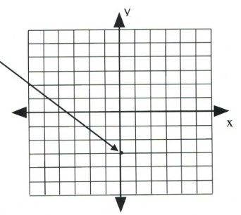
Now, place the next dot using the slope of 2.

A slope of 2 means that the line rises 2 for every 1 across.

Simply, [latex]m = 2[/latex] is the same as [latex]m = \dfrac{2}{1}[/latex], where [latex]\Delta y = 2[/latex] and [latex]\Delta x = 1[/latex].

Placing these points on the graph becomes a simple counting exercise, which is done as follows:

Once several dots have been drawn, draw a line through them, like so:

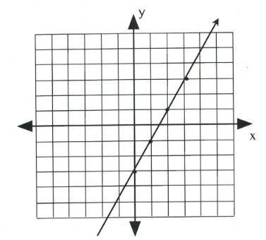
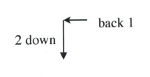
Note that dots can also be drawn in the reverse of what has been drawn here.

Slope is 2 when rise over run is [latex]\dfrac{2}{1}[/latex] or [latex]\dfrac{-2}{-1}[/latex], which would be drawn as follows:

Example 3.4.3

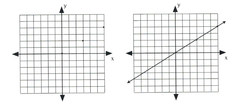
Graph the equation [latex]y = \dfrac{2}{3}x[/latex].

First, place a dot on the [latex]y[/latex]-intercept, [latex](0, 0)[/latex].

Now, place the dots according to the slope, [latex]\dfrac{2}{3}[/latex].

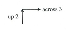
This will generate the following set of dots on the graph. All that remains is to draw a line through the dots.

The second method of drawing lines represented by linear equations and functions is to identify the two intercepts of the linear equation. Specifically, find [latex]x[/latex] when [latex]y = 0[/latex] and find [latex]y[/latex] when [latex]x = 0[/latex].

Example 3.4.4

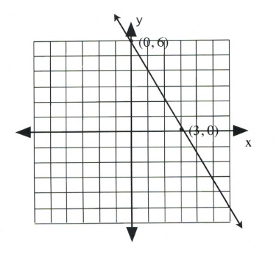
Graph the equation [latex]2x + y = 6[/latex].

To find the first coordinate, choose [latex]x = 0[/latex].

This yields:

[latex]\begin{array}{lllll} 2(0)&+&y&=&6 \\ &&y&=&6 \end{array}[/latex]

Coordinate is [latex](0, 6)[/latex].

Now choose [latex]y = 0[/latex].

[latex]\begin{array}{llrll} 2x&+&0&=&6 \\ &&2x&=&6 \\ &&x&=&\frac{6}{2} \text{ or } 3 \end{array}[/latex]

Coordinate is [latex](3, 0)[/latex].

Draw these coordinates on the graph and draw a line through them.

Example 3.4.5

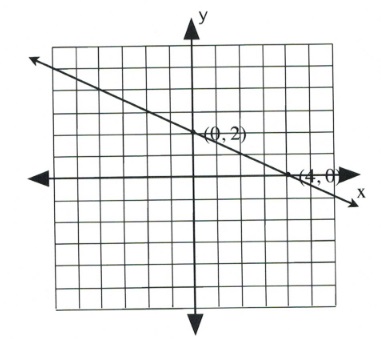
Graph the equation [latex]x + 2y = 4[/latex].

[latex]\begin{array}{llrll} (0)&+&2y&=&4 \\ &&y&=&\frac{4}{2} \text{ or } 2 \end{array}[/latex]

Coordinate is [latex](0, 2)[/latex].

[latex]\begin{array}{llrll} x&+&2(0)&=&4 \\ &&x&=&4 \end{array}[/latex]

Coordinate is [latex](4, 0)[/latex].

Example 3.4.6

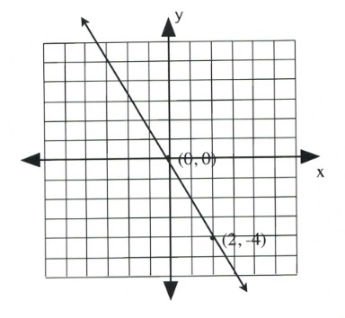
Graph the equation [latex]2x + y = 0[/latex].

[latex]\begin{array}{llrll} 2(0)&+&y&=&0 \\ &&y&=&0 \end{array}[/latex]

Coordinate is [latex](0, 0)[/latex].

Since the intercept is [latex](0, 0)[/latex], finding the other intercept yields the same coordinate. In this case, choose any value of convenience.

Choose [latex]x = 2[/latex].

[latex]\begin{array}{rlrlr} 2(2)&+&y&=&0 \\ 4&+&y&=&0 \\ -4&&&&-4 \\ \hline &&y&=&-4 \end{array}[/latex]

Coordinate is [latex](2, -4)[/latex].

For questions 1 to 10, sketch each linear equation using the slope-intercept method.

• [latex]y = -\dfrac{1}{4}x - 3[/latex]
• [latex]y = \dfrac{3}{2}x - 1[/latex]
• [latex]y = -\dfrac{5}{4}x - 4[/latex]
• [latex]y = -\dfrac{3}{5}x + 1[/latex]
• [latex]y = -\dfrac{4}{3}x + 2[/latex]
• [latex]y = \dfrac{5}{3}x + 4[/latex]
• [latex]y = \dfrac{3}{2}x - 5[/latex]
• [latex]y = -\dfrac{2}{3}x - 2[/latex]
• [latex]y = -\dfrac{4}{5}x - 3[/latex]
• [latex]y = \dfrac{1}{2}x[/latex]

For questions 11 to 20, sketch each linear equation using the [latex]x\text{-}[/latex] and [latex]y[/latex]-intercepts.

• [latex]x + 4y = -4[/latex]
• [latex]2x - y = 2[/latex]
• [latex]2x + y = 4[/latex]
• [latex]3x + 4y = 12[/latex]
• [latex]4x + 3y = -12[/latex]
• [latex]x + y = -5[/latex]
• [latex]3x + 2y = 6[/latex]
• [latex]x - y = -2[/latex]
• [latex]4x - y = -4[/latex]

For questions 21 to 28, sketch each linear equation using any method.

• [latex]y = -\dfrac{1}{2}x + 3[/latex]
• [latex]y = 2x - 1[/latex]
• [latex]y = -\dfrac{5}{4}x[/latex]
• [latex]y = -3x + 2[/latex]
• [latex]y = -\dfrac{3}{2}x + 1[/latex]
• [latex]y = \dfrac{1}{3}x - 3[/latex]
• [latex]y = \dfrac{3}{2}x + 2[/latex]
• [latex]y = 2x - 2[/latex]

For questions 29 to 40, reduce and sketch each linear equation using any method.

• [latex]y + 3 = -\dfrac{4}{5}x + 3[/latex]
• [latex]y - 4 = \dfrac{1}{2}x[/latex]
• [latex]x + 5y = -3 + 2y[/latex]
• [latex]3x - y = 4 + x - 2y[/latex]
• [latex]4x + 3y = 5 (x + y)[/latex]
• [latex]3x + 4y = 12 - 2y[/latex]
• [latex]2x - y = 2 - y \text{ (tricky)}[/latex]
• [latex]7x + 3y = 2(2x + 2y) + 6[/latex]
• [latex]x + y = -2x + 3[/latex]
• [latex]3x + 4y = 3y + 6[/latex]
• [latex]2(x + y) = -3(x + y) + 5[/latex]
• [latex]9x - y = 4x + 5[/latex]

Answer Key 3.4

Intermediate Algebra Copyright © 2020 by Terrance Berg is licensed under a Creative Commons Attribution-NonCommercial-ShareAlike 4.0 International License , except where otherwise noted.

Share This Book

3.1 Graph Linear Equations in Two Variables

Learning objectives.

By the end of this section, you will be able to:

• Plot points in a rectangular coordinate system
• Graph a linear equation by plotting points
• Graph vertical and horizontal lines
• Find the x- and y-intercepts
• Graph a line using the intercepts

Be Prepared 3.1

Before you get started, take this readiness quiz.

Evaluate 5 x − 4 5 x − 4 when x = −1 . x = −1 . If you missed this problem, review Example 1.6 .

Be Prepared 3.2

Evaluate 3 x − 2 y 3 x − 2 y when x = 4 , y = −3 . x = 4 , y = −3 . If you missed this problem, review Example 1.21 .

Be Prepared 3.3

Solve for y : 8 − 3 y = 20 . 8 − 3 y = 20 . If you missed this problem, review Example 2.2 .

Plot Points on a Rectangular Coordinate System

Just like maps use a grid system to identify locations, a grid system is used in algebra to show a relationship between two variables in a rectangular coordinate system. The rectangular coordinate system is also called the xy -plane or the “coordinate plane.”

The rectangular coordinate system is formed by two intersecting number lines, one horizontal and one vertical. The horizontal number line is called the x -axis. The vertical number line is called the y -axis. These axes divide a plane into four regions, called quadrants. The quadrants are identified by Roman numerals, beginning on the upper right and proceeding counterclockwise. See Figure 3.2 .

In the rectangular coordinate system, every point is represented by an ordered pair . The first number in the ordered pair is the x -coordinate of the point, and the second number is the y -coordinate of the point. The phrase “ordered pair” means that the order is important.

Ordered Pair

An ordered pair , ( x , y ) ( x , y ) gives the coordinates of a point in a rectangular coordinate system. The first number is the x -coordinate. The second number is the y -coordinate.

What is the ordered pair of the point where the axes cross? At that point both coordinates are zero, so its ordered pair is ( 0 , 0 ) . ( 0 , 0 ) . The point ( 0 , 0 ) ( 0 , 0 ) has a special name. It is called the origin .

The point ( 0 , 0 ) ( 0 , 0 ) is called the origin . It is the point where the x -axis and y -axis intersect.

We use the coordinates to locate a point on the xy -plane. Let’s plot the point ( 1 , 3 ) ( 1 , 3 ) as an example. First, locate 1 on the x -axis and lightly sketch a vertical line through x = 1 . x = 1 . Then, locate 3 on the y -axis and sketch a horizontal line through y = 3 . y = 3 . Now, find the point where these two lines meet—that is the point with coordinates ( 1 , 3 ) . ( 1 , 3 ) . See Figure 3.3 .

Notice that the vertical line through x = 1 x = 1 and the horizontal line through y = 3 y = 3 are not part of the graph. We just used them to help us locate the point ( 1 , 3 ) . ( 1 , 3 ) .

When one of the coordinate is zero, the point lies on one of the axes. In Figure 3.4 the point ( 0 , 4 ) ( 0 , 4 ) is on the y -axis and the point ( −2 , 0 ) ( −2 , 0 ) is on the x -axis.

Points on the Axes

Points with a y -coordinate equal to 0 are on the x -axis, and have coordinates ( a , 0 ) . ( a , 0 ) .

Points with an x -coordinate equal to 0 are on the y -axis, and have coordinates ( 0 , b ) . ( 0 , b ) .

Example 3.1

Plot each point in the rectangular coordinate system and identify the quadrant in which the point is located:

ⓐ ( −5 , 4 ) ( −5 , 4 ) ⓑ ( −3 , −4 ) ( −3 , −4 ) ⓒ ( 2 , −3 ) ( 2 , −3 ) ⓓ ( 0 , −1 ) ( 0 , −1 ) ⓔ ( 3 , 5 2 ) . ( 3 , 5 2 ) .

The first number of the coordinate pair is the x -coordinate, and the second number is the y -coordinate. To plot each point, sketch a vertical line through the x -coordinate and a horizontal line through the y -coordinate. Their intersection is the point. ⓐ Since x = −5 , x = −5 , the point is to the left of the y -axis. Also, since y = 4 , y = 4 , the point is above the x -axis. The point ( −5 , 4 ) ( −5 , 4 ) is in Quadrant II. ⓑ Since x = −3 , x = −3 , the point is to the left of the y -axis. Also, since y = −4 , y = −4 , the point is below the x -axis. The point ( −3 , −4 ) ( −3 , −4 ) is in Quadrant III. ⓒ Since x = 2 , x = 2 , the point is to the right of the y -axis. Since y = −3 , y = −3 , the point is below the x -axis. The point ( 2 , −3 ) ( 2 , −3 ) is in Quadrant IV. ⓓ Since x = 0 , x = 0 , the point whose coordinates are ( 0 , −1 ) ( 0 , −1 ) is on the y -axis. ⓔ Since x = 3 , x = 3 , the point is to the right of the y -axis. Since y = 5 2 , y = 5 2 , the point is above the x -axis. (It may be helpful to write 5 2 5 2 as a mixed number or decimal.) The point ( 3 , 5 2 ) ( 3 , 5 2 ) is in Quadrant I.

Plot each point in a rectangular coordinate system and identify the quadrant in which the point is located: ⓐ ( −2 , 1 ) ( −2 , 1 ) ⓑ ( −3 , −1 ) ( −3 , −1 ) ⓒ ( 4 , −4 ) ( 4 , −4 ) ⓓ ( −4 , 4 ) ( −4 , 4 ) ⓔ ( −4 , 3 2 ) ( −4 , 3 2 )

Plot each point in a rectangular coordinate system and identify the quadrant in which the point is located: ⓐ ( −4 , 1 ) ( −4 , 1 ) ⓑ ( −2 , 3 ) ( −2 , 3 ) ⓒ ( 2 , −5 ) ( 2 , −5 ) ⓓ ( −2 , 5 ) ( −2 , 5 ) ⓔ ( −3 , 5 2 ) ( −3 , 5 2 )

The signs of the x -coordinate and y -coordinate affect the location of the points. You may have noticed some patterns as you graphed the points in the previous example. We can summarize sign patterns of the quadrants in this way:

Up to now, all the equations you have solved were equations with just one variable. In almost every case, when you solved the equation you got exactly one solution. But equations can have more than one variable. Equations with two variables may be of the form A x + B y = C . A x + B y = C . An equation of this form is called a linear equation in two variables.

Linear Equation

An equation of the form A x + B y = C , A x + B y = C , where A and B are not both zero, is called a linear equation in two variables.

Here is an example of a linear equation in two variables, x and y .

The equation y = −3 x + 5 y = −3 x + 5 is also a linear equation. But it does not appear to be in the form A x + B y = C . A x + B y = C . We can use the Addition Property of Equality and rewrite it in A x + B y = C A x + B y = C form.

By rewriting y = −3 x + 5 y = −3 x + 5 as 3 x + y = 5 , 3 x + y = 5 , we can easily see that it is a linear equation in two variables because it is of the form A x + B y = C . A x + B y = C . When an equation is in the form A x + B y = C , A x + B y = C , we say it is in standard form of a linear equation .

Standard Form of Linear Equation

A linear equation is in standard form when it is written A x + B y = C . A x + B y = C .

Most people prefer to have A , B , and C be integers and A ≥ 0 A ≥ 0 when writing a linear equation in standard form, although it is not strictly necessary.

Linear equations have infinitely many solutions. For every number that is substituted for x there is a corresponding y value. This pair of values is a solution to the linear equation and is represented by the ordered pair ( x , y ) . ( x , y ) . When we substitute these values of x and y into the equation, the result is a true statement, because the value on the left side is equal to the value on the right side.

Solution of a Linear Equation in Two Variables

An ordered pair ( x , y ) ( x , y ) is a solution of the linear equation A x + B y = C , A x + B y = C , if the equation is a true statement when the x - and y -values of the ordered pair are substituted into the equation.

Linear equations have infinitely many solutions. We can plot these solutions in the rectangular coordinate system. The points will line up perfectly in a straight line. We connect the points with a straight line to get the graph of the equation. We put arrows on the ends of each side of the line to indicate that the line continues in both directions.

A graph is a visual representation of all the solutions of the equation. It is an example of the saying, “A picture is worth a thousand words.” The line shows you all the solutions to that equation. Every point on the line is a solution of the equation. And, every solution of this equation is on this line. This line is called the graph of the equation. Points not on the line are not solutions!

Graph of a Linear Equation

The graph of a linear equation A x + B y = C A x + B y = C is a straight line.

• Every point on the line is a solution of the equation.
• Every solution of this equation is a point on this line.

Example 3.2

The graph of y = 2 x − 3 y = 2 x − 3 is shown.

For each ordered pair, decide:

ⓐ Is the ordered pair a solution to the equation?

ⓑ Is the point on the line?

A: ( 0 , −3 ) ( 0 , −3 ) B: ( 3 , 3 ) ( 3 , 3 ) C: ( 2 , −3 ) ( 2 , −3 ) D: ( −1 , −5 ) ( −1 , −5 )

Substitute the x - and y -values into the equation to check if the ordered pair is a solution to the equation. ⓐ

ⓑ Plot the points ( 0 , −3 ) , ( 0 , −3 ) , ( 3 , 3 ) , ( 3 , 3 ) , ( 2 , −3 ) , ( 2 , −3 ) , and ( −1 , −5 ) . ( −1 , −5 ) .

The points ( 0 , 3 ) , ( 0 , 3 ) , ( 3 , −3 ) , ( 3 , −3 ) , and ( −1 , −5 ) ( −1 , −5 ) are on the line y = 2 x − 3 , y = 2 x − 3 , and the point ( 2 , −3 ) ( 2 , −3 ) is not on the line. The points that are solutions to y = 2 x − 3 y = 2 x − 3 are on the line, but the point that is not a solution is not on the line.

Use graph of y = 3 x − 1 . y = 3 x − 1 . For each ordered pair, decide:

ⓐ Is the ordered pair a solution to the equation? ⓑ Is the point on the line?

A ( 0 , −1 ) ( 0 , −1 ) B ( 2 , 5 ) ( 2 , 5 )

A ( 3 , −1 ) ( 3 , −1 ) B ( −1 , −4 ) ( −1 , −4 )

Graph a Linear Equation by Plotting Points

There are several methods that can be used to graph a linear equation. The first method we will use is called plotting points, or the Point-Plotting Method. We find three points whose coordinates are solutions to the equation and then plot them in a rectangular coordinate system. By connecting these points in a line, we have the graph of the linear equation.

Example 3.3

How to graph a linear equation by plotting points.

Graph the equation y = 2 x + 1 y = 2 x + 1 by plotting points.

Graph the equation by plotting points: y = 2 x − 3 . y = 2 x − 3 .

Graph the equation by plotting points: y = −2 x + 4 . y = −2 x + 4 .

The steps to take when graphing a linear equation by plotting points are summarized here.

Graph a linear equation by plotting points.

• Step 1. Find three points whose coordinates are solutions to the equation. Organize them in a table.
• Step 2. Plot the points in a rectangular coordinate system. Check that the points line up. If they do not, carefully check your work.
• Step 3. Draw the line through the three points. Extend the line to fill the grid and put arrows on both ends of the line.

It is true that it only takes two points to determine a line, but it is a good habit to use three points. If you only plot two points and one of them is incorrect, you can still draw a line but it will not represent the solutions to the equation. It will be the wrong line.

If you use three points, and one is incorrect, the points will not line up. This tells you something is wrong and you need to check your work. Look at the difference between these illustrations.

When an equation includes a fraction as the coefficient of x x , we can still substitute any numbers for x . But the arithmetic is easier if we make “good” choices for the values of x . This way we will avoid fractional answers, which are hard to graph precisely.

Example 3.4

Graph the equation: y = 1 2 x + 3 . y = 1 2 x + 3 .

Find three points that are solutions to the equation. Since this equation has the fraction 1 2 1 2 as a coefficient of x , we will choose values of x carefully. We will use zero as one choice and multiples of 2 for the other choices. Why are multiples of two a good choice for values of x ? By choosing multiples of 2 the multiplication by 1 2 1 2 simplifies to a whole number

The points are shown in Table 3.1 .

Plot the points, check that they line up, and draw the line.

Graph the equation: y = 1 3 x − 1 . y = 1 3 x − 1 .

Graph the equation: y = 1 4 x + 2 . y = 1 4 x + 2 .

Graph Vertical and Horizontal Lines

Some linear equations have only one variable. They may have just x and no y , or just y without an x . This changes how we make a table of values to get the points to plot.

Let’s consider the equation x = −3 . x = −3 . This equation has only one variable, x . The equation says that x is always equal to −3 , −3 , so its value does not depend on y . No matter what is the value of y , the value of x is always −3 . −3 .

So to make a table of values, write −3 −3 in for all the x -values. Then choose any values for y . Since x does not depend on y , you can choose any numbers you like. But to fit the points on our coordinate graph, we’ll use 1, 2, and 3 for the y -coordinates. See Table 3.2 .

Plot the points from the table and connect them with a straight line. Notice that we have graphed a vertical line .

What if the equation has y but no x ? Let’s graph the equation y = 4 . y = 4 . This time the y- value is a constant, so in this equation, y does not depend on x . Fill in 4 for all the y ’s in Table 3.3 and then choose any values for x . We’ll use 0, 2, and 4 for the x -coordinates.

In this figure, we have graphed a horizontal line passing through the y -axis at 4.

Vertical and Horizontal Lines

A vertical line is the graph of an equation of the form x = a . x = a .

The line passes through the x -axis at ( a , 0 ) . ( a , 0 ) .

A horizontal line is the graph of an equation of the form y = b . y = b .

The line passes through the y -axis at ( 0 , b ) . ( 0 , b ) .

Example 3.5

Graph: ⓐ x = 2 x = 2 ⓑ y = −1 . y = −1 .

ⓐ The equation has only one variable, x , and x is always equal to 2. We create a table where x is always 2 and then put in any values for y . The graph is a vertical line passing through the x -axis at 2.

ⓑ Similarly, the equation y = −1 y = −1 has only one variable, y . The value of y is constant. All the ordered pairs in the next table have the same y -coordinate. The graph is a horizontal line passing through the y -axis at −1 . −1 .

Graph the equations: ⓐ x = 5 x = 5 ⓑ y = −4 . y = −4 .

Try It 3.10

Graph the equations: ⓐ x = −2 x = −2 ⓑ y = 3 . y = 3 .

What is the difference between the equations y = 4 x y = 4 x and y = 4 ? y = 4 ?

The equation y = 4 x y = 4 x has both x and y . The value of y depends on the value of x , so the y -coordinate changes according to the value of x . The equation y = 4 y = 4 has only one variable. The value of y is constant, it does not depend on the value of x , so the y -coordinate is always 4.

Notice, in the graph, the equation y = 4 x y = 4 x gives a slanted line, while y = 4 y = 4 gives a horizontal line.

Example 3.6

Graph y = −3 x y = −3 x and y = −3 y = −3 in the same rectangular coordinate system.

We notice that the first equation has the variable x , while the second does not. We make a table of points for each equation and then graph the lines. The two graphs are shown.

Try It 3.11

Graph the equations in the same rectangular coordinate system: y = −4 x y = −4 x and y = −4 . y = −4 .

Try It 3.12

Graph the equations in the same rectangular coordinate system: y = 3 y = 3 and y = 3 x . y = 3 x .

Find x - and y -intercepts

Every linear equation can be represented by a unique line that shows all the solutions of the equation. We have seen that when graphing a line by plotting points, you can use any three solutions to graph. This means that two people graphing the line might use different sets of three points.

At first glance, their two lines might not appear to be the same, since they would have different points labeled. But if all the work was done correctly, the lines should be exactly the same. One way to recognize that they are indeed the same line is to look at where the line crosses the x -axis and the y -axis. These points are called the intercepts of a line .

Intercepts of a Line

The points where a line crosses the x -axis and the y -axis are called the intercepts of the line .

Let’s look at the graphs of the lines.

First, notice where each of these lines crosses the x -axis. See Table 3.4 .

Now, let’s look at the points where these lines cross the y -axis.

Do you see a pattern?

For each line, the y -coordinate of the point where the line crosses the x -axis is zero. The point where the line crosses the x -axis has the form ( a , 0 ) ( a , 0 ) and is called the x-intercept of the line. The x -intercept occurs when y is zero.

In each line, the x - coordinate of the point where the line crosses the y -axis is zero. The point where the line crosses the y -axis has the form ( 0 , b ) ( 0 , b ) and is called the y-intercept of the line. The y -intercept occurs when x is zero.

x -intercept and y -intercept of a Line

The x -intercept is the point ( a , 0 ) ( a , 0 ) where the line crosses the x -axis.

The y -intercept is the point ( 0 , b ) ( 0 , b ) where the line crosses the y -axis.

Example 3.7

Find the x - and y -intercepts on each graph shown.

ⓐ The graph crosses the x -axis at the point ( 4 , 0 ) . ( 4 , 0 ) . The x- intercept is ( 4 , 0 ) . ( 4 , 0 ) . The graph crosses the y -axis at the point ( 0 , 2 ) . ( 0 , 2 ) . The y -intercept is ( 0 , 2 ) . ( 0 , 2 ) . ⓑ The graph crosses the x -axis at the point ( 2 , 0 ) . ( 2 , 0 ) . The x -intercept is ( 2 , 0 ) . ( 2 , 0 ) . The graph crosses the y -axis at the point ( 0 , −6 ) . ( 0 , −6 ) . The y -intercept is ( 0 , −6 ) . ( 0 , −6 ) . ⓒ The graph crosses the x -axis at the point ( −5 , 0 ) . ( −5 , 0 ) . The x -intercept is ( −5 , 0 ) . ( −5 , 0 ) . The graph crosses the y -axis at the point ( 0 , −5 ) . ( 0 , −5 ) . The y -intercept is ( 0 , −5 ) . ( 0 , −5 ) .

Try It 3.13

Find the x - and y -intercepts on the graph.

Try It 3.14

Recognizing that the x -intercept occurs when y is zero and that the y -intercept occurs when x is zero, gives us a method to find the intercepts of a line from its equation. To find the x -intercept, let y = 0 y = 0 and solve for x . To find the y -intercept, let x = 0 x = 0 and solve for y .

Find the x - and y -intercepts from the Equation of a Line

Use the equation of the line. To find:

• the x -intercept of the line, let y = 0 y = 0 and solve for x .
• the y -intercept of the line, let x = 0 x = 0 and solve for y .

Example 3.8

Find the intercepts of 2 x + y = 8 . 2 x + y = 8 .

We will let y = 0 y = 0 to find the x -intercept, and let x = 0 x = 0 to find the y -intercept. We will fill in a table, which reminds us of what we need to find.

The intercepts are the points ( 4 , 0 ) ( 4 , 0 ) and ( 0 , 8 ) ( 0 , 8 ) as shown in the table.

Try It 3.15

Find the intercepts: 3 x + y = 12 . 3 x + y = 12 .

Try It 3.16

Find the intercepts: x + 4 y = 8 . x + 4 y = 8 .

Graph a Line Using the Intercepts

To graph a linear equation by plotting points, you need to find three points whose coordinates are solutions to the equation. You can use the x- and y- intercepts as two of your three points. Find the intercepts, and then find a third point to ensure accuracy. Make sure the points line up—then draw the line. This method is often the quickest way to graph a line.

Example 3.9

How to graph a line using the intercepts.

Graph – x + 2 y = 6 – x + 2 y = 6 using the intercepts.

Try It 3.17

Graph using the intercepts: x – 2 y = 4 . x – 2 y = 4 .

Try It 3.18

Graph using the intercepts: – x + 3 y = 6 . – x + 3 y = 6 .

The steps to graph a linear equation using the intercepts are summarized here.

Graph a linear equation using the intercepts.

• Let y = 0 y = 0 and solve for x .
• Let x = 0 x = 0 and solve for y .
• Step 2. Find a third solution to the equation.
• Step 3. Plot the three points and check that they line up.
• Step 4. Draw the line.

Example 3.10

Graph 4 x − 3 y = 12 4 x − 3 y = 12 using the intercepts.

Find the intercepts and a third point.

We list the points in the table and show the graph.

Try It 3.19

Graph using the intercepts: 5 x − 2 y = 10 . 5 x − 2 y = 10 .

Try It 3.20

Graph using the intercepts: 3 x − 4 y = 12 . 3 x − 4 y = 12 .

When the line passes through the origin, the x -intercept and the y -intercept are the same point.

Example 3.11

Graph y = 5 x y = 5 x using the intercepts.

This line has only one intercept. It is the point ( 0 , 0 ) . ( 0 , 0 ) . To ensure accuracy, we need to plot three points. Since the x - and y -intercepts are the same point, we need two more points to graph the line.

The resulting three points are summarized in the table.

Plot the three points, check that they line up, and draw the line.

Try It 3.21

Graph using the intercepts: y = 4 x . y = 4 x .

Try It 3.22

Graph the intercepts: y = − x . y = − x .

Section 3.1 Exercises

Practice makes perfect.

Plot Points in a Rectangular Coordinate System

In the following exercises, plot each point in a rectangular coordinate system and identify the quadrant in which the point is located.

ⓐ ( −4 , 2 ) ( −4 , 2 ) ⓑ ( −1 , −2 ) ( −1 , −2 ) ⓒ ( 3 , −5 ) ( 3 , −5 ) ⓓ ( −3 , 0 ) ( −3 , 0 ) ⓔ ( 5 3 , 2 ) ( 5 3 , 2 )

ⓐ ( −2 , −3 ) ( −2 , −3 ) ⓑ ( 3 , −3 ) ( 3 , −3 ) ⓒ ( −4 , 1 ) ( −4 , 1 ) ⓓ ( 4 , −1 ) ( 4 , −1 ) ⓔ ( 3 2 , 1 ) ( 3 2 , 1 )

ⓐ ( 3 , −1 ) ( 3 , −1 ) ⓑ ( −3 , 1 ) ( −3 , 1 ) ⓒ ( −2 , 0 ) ( −2 , 0 ) ⓓ ( −4 , −3 ) ( −4 , −3 ) ⓔ ( 1 , 14 5 ) ( 1 , 14 5 )

ⓐ ( −1 , 1 ) ( −1 , 1 ) ⓑ ( −2 , −1 ) ( −2 , −1 ) ⓒ ( 2 , 0 ) ( 2 , 0 ) ⓓ ( 1 , −4 ) ( 1 , −4 ) ⓔ ( 3 , 7 2 ) ( 3 , 7 2 )

In the following exercises, for each ordered pair, decide

ⓐ is the ordered pair a solution to the equation? ⓑ is the point on the line?

y = x + 2 ; y = x + 2 ; A: ( 0 , 2 ) ; ( 0 , 2 ) ; B: ( 1 , 2 ) ; ( 1 , 2 ) ; C: ( −1 , 1 ) ; ( −1 , 1 ) ; D: ( −3 , −1 ) . ( −3 , −1 ) .

y = x − 4 ; y = x − 4 ; A: ( 0 , −4 ) ; ( 0 , −4 ) ; B: ( 3 , −1 ) ; ( 3 , −1 ) ; C: ( 2 , 2 ) ; ( 2 , 2 ) ; D: ( 1 , −5 ) . ( 1 , −5 ) .

y = 1 2 x − 3 ; y = 1 2 x − 3 ; A: ( 0 , −3 ) ; ( 0 , −3 ) ; B: ( 2 , −2 ) ; ( 2 , −2 ) ; C: ( −2 , −4 ) ; ( −2 , −4 ) ; D: ( 4 , 1 ) ( 4 , 1 )

y = 1 3 x + 2 ; y = 1 3 x + 2 ; A: ( 0 , 2 ) ; ( 0 , 2 ) ; B: ( 3 , 3 ) ; ( 3 , 3 ) ; C: ( −3 , 2 ) ; ( −3 , 2 ) ; D: ( −6 , 0 ) . ( −6 , 0 ) .

In the following exercises, graph by plotting points.

y = x + 2 y = x + 2

y = x − 3 y = x − 3

y = 3 x − 1 y = 3 x − 1

y = −2 x + 2 y = −2 x + 2

y = − x − 3 y = − x − 3

y = − x − 2 y = − x − 2

y = 2 x y = 2 x

y = −2 x y = −2 x

y = 1 2 x + 2 y = 1 2 x + 2

y = 1 3 x − 1 y = 1 3 x − 1

y = 4 3 x − 5 y = 4 3 x − 5

y = 3 2 x − 3 y = 3 2 x − 3

y = − 2 5 x + 1 y = − 2 5 x + 1

y = − 4 5 x − 1 y = − 4 5 x − 1

y = − 3 2 x + 2 y = − 3 2 x + 2

y = − 5 3 x + 4 y = − 5 3 x + 4

Graph Vertical and Horizontal lines

In the following exercises, graph each equation.

ⓐ x = 4 x = 4 ⓑ y = 3 y = 3

ⓐ x = 3 x = 3 ⓑ y = 1 y = 1

ⓐ x = −2 x = −2 ⓑ y = −5 y = −5

ⓐ x = −5 x = −5 ⓑ y = −2 y = −2

In the following exercises, graph each pair of equations in the same rectangular coordinate system.

y = 2 x y = 2 x and y = 2 y = 2

y = 5 x y = 5 x and y = 5 y = 5

y = − 1 2 x y = − 1 2 x and y = − 1 2 y = − 1 2

y = − 1 3 x y = − 1 3 x and y = − 1 3 y = − 1 3

Find x- and y- Intercepts

In the following exercises, find the x - and y -intercepts on each graph.

In the following exercises, find the intercepts for each equation.

x − y = 5 x − y = 5

x − y = −4 x − y = −4

3 x + y = 6 3 x + y = 6

x − 2 y = 8 x − 2 y = 8

4 x − y = 8 4 x − y = 8

5 x − y = 5 5 x − y = 5

2 x + 5 y = 10 2 x + 5 y = 10

3 x − 2 y = 12 3 x − 2 y = 12

In the following exercises, graph using the intercepts.

− x + 4 y = 8 − x + 4 y = 8

x + 2 y = 4 x + 2 y = 4

x + y = −3 x + y = −3

4 x + y = 4 4 x + y = 4

3 x + y = 3 3 x + y = 3

3 x − y = −6 3 x − y = −6

2 x − y = −8 2 x − y = −8

2 x + 4 y = 12 2 x + 4 y = 12

3 x − 2 y = 6 3 x − 2 y = 6

2 x − 5 y = −20 2 x − 5 y = −20

3 x − 4 y = −12 3 x − 4 y = −12

y = 5 x y = 5 x

y = x y = x

y = − x y = − x

Mixed Practice

y = 3 2 x y = 3 2 x

y = − 2 3 x y = − 2 3 x

y = − 1 2 x + 3 y = − 1 2 x + 3

y = 1 4 x − 2 y = 1 4 x − 2

4 x + y = 2 4 x + y = 2

5 x + 2 y = 10 5 x + 2 y = 10

y = −1 y = −1

x = 3 x = 3

Writing Exercises

Explain how you would choose three x -values to make a table to graph the line y = 1 5 x − 2 . y = 1 5 x − 2 .

What is the difference between the equations of a vertical and a horizontal line?

Do you prefer to use the method of plotting points or the method using the intercepts to graph the equation 4 x + y = −4 ? 4 x + y = −4 ? Why?

Do you prefer to use the method of plotting points or the method using the intercepts to graph the equation y = 2 3 x − 2 ? y = 2 3 x − 2 ? Why?

ⓐ After completing the exercises, use this checklist to evaluate your mastery of the objectives of this section.

ⓑ If most of your checks were:

Confidently. Congratulations! You have achieved the objectives in this section. Reflect on the study skills you used so that you can continue to use them. What did you do to become confident of your ability to do these things? Be specific.

With some help. This must be addressed quickly because topics you do not master become potholes in your road to success. In math every topic builds upon previous work. It is important to make sure you have a strong foundation before you move on. Whom can you ask for help?Your fellow classmates and instructor are good resources. Is there a place on campus where math tutors are available? Can your study skills be improved?

No, I don’t get it. This is a warning sign and you must address it. You should get help right away or you will quickly be overwhelmed. See your instructor as soon as you can to discuss your situation. Together you can come up with a plan to get you the help you need.

As an Amazon Associate we earn from qualifying purchases.

This book may not be used in the training of large language models or otherwise be ingested into large language models or generative AI offerings without OpenStax's permission.

Want to cite, share, or modify this book? This book uses the Creative Commons Attribution License and you must attribute OpenStax.

Access for free at https://openstax.org/books/intermediate-algebra-2e/pages/1-introduction

• Authors: Lynn Marecek, Andrea Honeycutt Mathis
• Publisher/website: OpenStax
• Book title: Intermediate Algebra 2e
• Publication date: May 6, 2020
• Location: Houston, Texas
• Book URL: https://openstax.org/books/intermediate-algebra-2e/pages/1-introduction
• Section URL: https://openstax.org/books/intermediate-algebra-2e/pages/3-1-graph-linear-equations-in-two-variables

© Jan 23, 2024 OpenStax. Textbook content produced by OpenStax is licensed under a Creative Commons Attribution License . The OpenStax name, OpenStax logo, OpenStax book covers, OpenStax CNX name, and OpenStax CNX logo are not subject to the Creative Commons license and may not be reproduced without the prior and express written consent of Rice University.

• school Campus Bookshelves
• menu_book Bookshelves
• perm_media Learning Objects
• login Login
• how_to_reg Request Instructor Account
• hub Instructor Commons

Margin Size

• Download Page (PDF)
• Download Full Book (PDF)
• Periodic Table
• Physics Constants
• Scientific Calculator
• Reference & Cite
• Tools expand_more
• Readability

selected template will load here

This action is not available.

3.4: Graph Using Intercepts

• Last updated
• Save as PDF
• Page ID 4276

\( \newcommand{\vecs}[1]{\overset { \scriptstyle \rightharpoonup} {\mathbf{#1}} } \)

\( \newcommand{\vecd}[1]{\overset{-\!-\!\rightharpoonup}{\vphantom{a}\smash {#1}}} \)

\( \newcommand{\id}{\mathrm{id}}\) \( \newcommand{\Span}{\mathrm{span}}\)

( \newcommand{\kernel}{\mathrm{null}\,}\) \( \newcommand{\range}{\mathrm{range}\,}\)

\( \newcommand{\RealPart}{\mathrm{Re}}\) \( \newcommand{\ImaginaryPart}{\mathrm{Im}}\)

\( \newcommand{\Argument}{\mathrm{Arg}}\) \( \newcommand{\norm}[1]{\| #1 \|}\)

\( \newcommand{\inner}[2]{\langle #1, #2 \rangle}\)

\( \newcommand{\Span}{\mathrm{span}}\)

\( \newcommand{\id}{\mathrm{id}}\)

\( \newcommand{\kernel}{\mathrm{null}\,}\)

\( \newcommand{\range}{\mathrm{range}\,}\)

\( \newcommand{\RealPart}{\mathrm{Re}}\)

\( \newcommand{\ImaginaryPart}{\mathrm{Im}}\)

\( \newcommand{\Argument}{\mathrm{Arg}}\)

\( \newcommand{\norm}[1]{\| #1 \|}\)

\( \newcommand{\Span}{\mathrm{span}}\) \( \newcommand{\AA}{\unicode[.8,0]{x212B}}\)

\( \newcommand{\vectorA}[1]{\vec{#1}}      % arrow\)

\( \newcommand{\vectorAt}[1]{\vec{\text{#1}}}      % arrow\)

\( \newcommand{\vectorB}[1]{\overset { \scriptstyle \rightharpoonup} {\mathbf{#1}} } \)

\( \newcommand{\vectorC}[1]{\textbf{#1}} \)

\( \newcommand{\vectorD}[1]{\overrightarrow{#1}} \)

\( \newcommand{\vectorDt}[1]{\overrightarrow{\text{#1}}} \)

\( \newcommand{\vectE}[1]{\overset{-\!-\!\rightharpoonup}{\vphantom{a}\smash{\mathbf {#1}}}} \)

• school Campus Bookshelves
• menu_book Bookshelves
• perm_media Learning Objects
• login Login
• how_to_reg Request Instructor Account
• hub Instructor Commons

Margin Size

• Download Page (PDF)
• Download Full Book (PDF)
• Periodic Table
• Physics Constants
• Scientific Calculator
• Reference & Cite
• Tools expand_more
• Readability

selected template will load here

This action is not available.

3.5: Use the Slope–Intercept Form of an Equation of a Line

• Last updated
• Save as PDF
• Page ID 54981

\( \newcommand{\vecs}[1]{\overset { \scriptstyle \rightharpoonup} {\mathbf{#1}} } \)

\( \newcommand{\vecd}[1]{\overset{-\!-\!\rightharpoonup}{\vphantom{a}\smash {#1}}} \)

\( \newcommand{\id}{\mathrm{id}}\) \( \newcommand{\Span}{\mathrm{span}}\)

( \newcommand{\kernel}{\mathrm{null}\,}\) \( \newcommand{\range}{\mathrm{range}\,}\)

\( \newcommand{\RealPart}{\mathrm{Re}}\) \( \newcommand{\ImaginaryPart}{\mathrm{Im}}\)

\( \newcommand{\Argument}{\mathrm{Arg}}\) \( \newcommand{\norm}[1]{\| #1 \|}\)

\( \newcommand{\inner}[2]{\langle #1, #2 \rangle}\)

\( \newcommand{\Span}{\mathrm{span}}\)

\( \newcommand{\id}{\mathrm{id}}\)

\( \newcommand{\kernel}{\mathrm{null}\,}\)

\( \newcommand{\range}{\mathrm{range}\,}\)

\( \newcommand{\RealPart}{\mathrm{Re}}\)

\( \newcommand{\ImaginaryPart}{\mathrm{Im}}\)

\( \newcommand{\Argument}{\mathrm{Arg}}\)

\( \newcommand{\norm}[1]{\| #1 \|}\)

\( \newcommand{\Span}{\mathrm{span}}\) \( \newcommand{\AA}{\unicode[.8,0]{x212B}}\)

\( \newcommand{\vectorA}[1]{\vec{#1}}      % arrow\)

\( \newcommand{\vectorAt}[1]{\vec{\text{#1}}}      % arrow\)

\( \newcommand{\vectorB}[1]{\overset { \scriptstyle \rightharpoonup} {\mathbf{#1}} } \)

\( \newcommand{\vectorC}[1]{\textbf{#1}} \)

\( \newcommand{\vectorD}[1]{\overrightarrow{#1}} \)

\( \newcommand{\vectorDt}[1]{\overrightarrow{\text{#1}}} \)

\( \newcommand{\vectE}[1]{\overset{-\!-\!\rightharpoonup}{\vphantom{a}\smash{\mathbf {#1}}}} \)

Learning Objectives

By the end of this section, you will be able to:

• Recognize the relation between the graph and the slope–intercept form of an equation of a line
• Identify the slope and y-intercept form of an equation of a line
• Graph a line using its slope and intercept
• Choose the most convenient method to graph a line
• Graph and interpret applications of slope–intercept
• Use slopes to identify parallel lines
• Use slopes to identify perpendicular lines

Before you get started, take this readiness quiz.

• Add: \(\frac{x}{4} + \frac{1}{4}\). If you missed this problem, review Exercise 1.7.1 .
• Find the reciprocal of \(\frac{3}{7}\). If you missed this problem, review Exercise 1.6.19 .
• Solve \(2x−3y=12\) for \(y\). If you missed this problem, review Exercise 2.6.16 .

Recognize the Relation Between the Graph and the Slope–Intercept Form of an Equation of a Line

We have graphed linear equations by plotting points, using intercepts, recognizing horizontal and vertical lines, and using the point–slope method. Once we see how an equation in slope–intercept form and its graph are related, we’ll have one more method we can use to graph lines.

In Graph Linear Equations in Two Variables , we graphed the line of the equation \(y=12x+3\) by plotting points. See Figure \(\PageIndex{1}\). Let’s find the slope of this line.

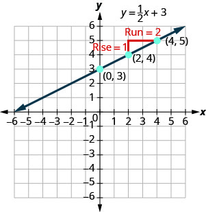
The red lines show us the rise is \(1\) and the run is \(2\). Substituting into the slope formula:

\[\begin{aligned} m &=\frac{\text { rise }}{\text { run }} \\ m &=\frac{1}{2} \end{aligned}\]

What is the \(y\)-intercept of the line? The \(y\)-intercept is where the line crosses the \(y\)-axis, so \(y\)-intercept is \((0,3)\). The equation of this line is:

Notice, the line has:

When a linear equation is solved for \(y\), the coefficient of the \(x\)-term is the slope and the constant term is the \(y\)-coordinate of the \(y\)-intercept. We say that the equation \(y=\frac{1}{2}x+3\) is in slope–intercept form.

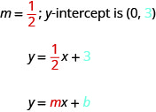
SLOPE-INTERCEPT FORM OF AN EQUATION OF A LINE

The slope–intercept form of an equation of a line with slope \(m\) and \(y\)-intercept, \((0,b)\) is,

Sometimes the slope–intercept form is called the “ y -form.”

Example \(\PageIndex{1}\)

Use the graph to find the slope and \(y\)-intercept of the line, \(y=2x+1\).

Compare these values to the equation \(y=mx+b\).

To find the slope of the line, we need to choose two points on the line. We’ll use the points \((0,1)\) and \((1,3)\).

The slope is the same as the coefficient of \(x\) and the \(y\)-coordinate of the \(y\)-intercept is the same as the constant term.

Try It \(\PageIndex{2}\)

Use the graph to find the slope and \(y\)-intercept of the line \(y=\frac{2}{3}x−1\). Compare these values to the equation \(y=mx+b\).

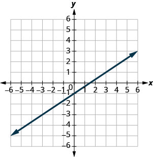
slope \(m = \frac{2}{3}\) and \(y\)-intercept \((0,−1)\)

Try It \(\PageIndex{3}\)

Use the graph to find the slope and \(y\)-intercept of the line \(y=\frac{1}{2}x+3\). Compare these values to the equation \(y=mx+b\).

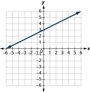
slope \(m = \frac{1}{2}\) and \(y\)-intercept \((0,3)\)

Identify the Slope and \(y\)-Intercept From an Equation of a Line

In Understand Slope of a Line , we graphed a line using the slope and a point. When we are given an equation in slope–intercept form, we can use the \(y\)-intercept as the point, and then count out the slope from there. Let’s practice finding the values of the slope and \(y\)-intercept from the equation of a line.

Example \(\PageIndex{4}\)

Identify the slope and \(y\)-intercept of the line with equation \(y=−3x+5\).

We compare our equation to the slope–intercept form of the equation.

Try It \(\PageIndex{5}\)

Identify the slope and \(y\)-intercept of the line \(y=\frac{2}{5}x−1\).

slope \(\frac{2}{5}\); \(y\)-intercept (0,−1)

Try It \(\PageIndex{6}\)

Identify the slope and \(y\)-intercept of the line \(y=−\frac{4}{3}x+1\).

slope \(-\frac{4}{3}\); \(y\)-intercept (0,1)

When an equation of a line is not given in slope–intercept form, our first step will be to solve the equation for \(y\).

Example \(\PageIndex{7}\)

Identify the slope and \(y\)-intercept of the line with equation \(x+2y=6\).

This equation is not in slope–intercept form. In order to compare it to the slope–intercept form we must first solve the equation for \(y\).

Try It \(\PageIndex{8}\)

Identify the slope and \(y\)-intercept of the line \(x+4y=8\).

slope \(-\frac{1}{4}\); \(y\)-intercept (0,2)

Try It \(\PageIndex{9}\)

Identify the slope and \(y\)-intercept of the line \(3x+2y=12\).

slope \(-\frac{3}{2}\); \(y\)-intercept (0,6)

Graph a Line Using its Slope and Intercept

Now that we know how to find the slope and \(y\)-intercept of a line from its equation, we can graph the line by plotting the \(y\)-intercept and then using the slope to find another point.

Example \(\PageIndex{10}\): How to Graph a Line Using its Slope and Intercept

Graph the line of the equation \(y=4x−2\) using its slope and \(y\)-intercept.

Try It \(\PageIndex{11}\)

Graph the line of the equation \(y=4x+1\) using its slope and \(y\)-intercept.

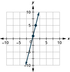
Try It \(\PageIndex{12}\)

Graph the line of the equation \(y=2x−3\) using its slope and \(y\)-intercept.

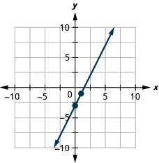
GRAPH A LINE USING ITS SLOPE AND \(y\)-INTERCEPT.

• Find the slope-intercept form of the equation of the line.
• Identify the slope and \(y\)-intercept.
• Plot the \(y\)-intercept.
• Use the slope formula \(\frac{\text{rise}}{\text{run}}\) to identify the rise and the run.
• Starting at the \(y\)-intercept, count out the rise and run to mark the second point.
• Connect the points with a line.

Example \(\PageIndex{13}\)

Graph the line of the equation \(y=−x+4\) using its slope and \(y\)-intercept.

\(\begin{array}{l}{y=-x+4} \\ {0\stackrel{?}{=}-4+4} \\ {0=0\checkmark}\end{array}\)

Try It \(\PageIndex{14}\)

Graph the line of the equation \(y=−x−3\) using its slope and \(y\)-intercept.

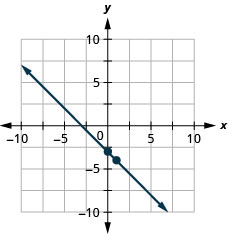
Try It \(\PageIndex{15}\)

Graph the line of the equation \(y=−x−1\) using its slope and \(y\)-intercept.

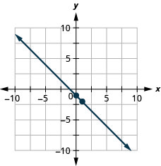
Example \(\PageIndex{16}\)

Graph the line of the equation \(y=−\frac{2}{3}x−3\) using its slope and \(y\)-intercept.

Try It \(\PageIndex{17}\)

Graph the line of the equation \(y=−\frac{5}{2}x+1\) using its slope and \(y\)-intercept.

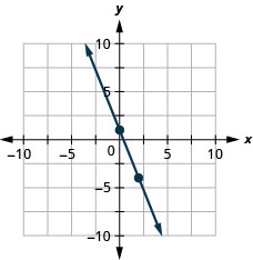
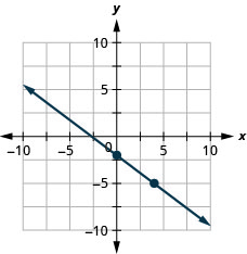
Try It \(\PageIndex{18}\)

Graph the line of the equation \(y=−\frac{3}{4}x−2\) using its slope and \(y\)-intercept.

Example \(\PageIndex{19}\)

Graph the line of the equation \(4x−3y=12\) using its slope and \(y\)-intercept.

Try It \(\PageIndex{20}\)

Graph the line of the equation \(2x−y=6\) using its slope and \(y\)-intercept.

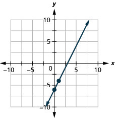
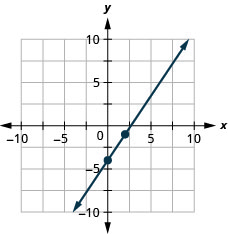
Try It \(\PageIndex{21}\)

Graph the line of the equation \(3x−2y=8\) using its slope and \(y\)-intercept.

We have used a grid with \(x\) and \(y\) both going from about \(−10\) to \(10\) for all the equations we’ve graphed so far. Not all linear equations can be graphed on this small grid. Often, especially in applications with real-world data, we’ll need to extend the axes to bigger positive or smaller negative numbers.

Example \(\PageIndex{22}\)

Graph the line of the equation \(y=0.2x+45\) using its slope and \(y\)-intercept.

We’ll use a grid with the axes going from about \(−80\) to \(80\).

Try It \(\PageIndex{23}\)

Graph the line of the equation \(y=0.5x+25\) using its slope and \(y\)-intercept.

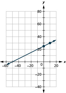
Try It \(\PageIndex{24}\)

Graph the line of the equation \(y=0.1x−30\) using its slope and \(y\)-intercept.

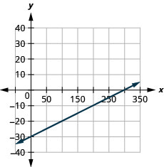
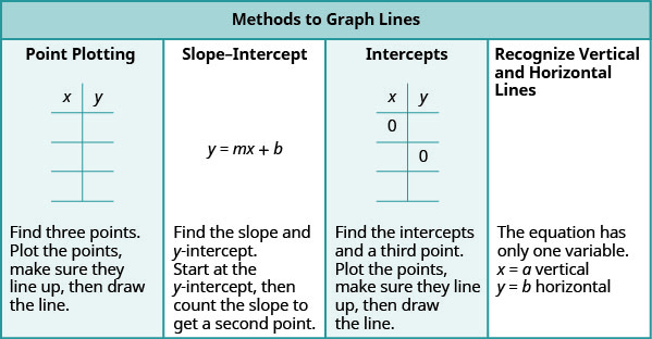
Now that we have graphed lines by using the slope and \(y\)-intercept, let’s summarize all the methods we have used to graph lines. See Figure \(\PageIndex{2}\).

Choose the Most Convenient Method to Graph a Line

Now that we have seen several methods we can use to graph lines, how do we know which method to use for a given equation?

While we could plot points, use the slope–intercept form, or find the intercepts for any equation, if we recognize the most convenient way to graph a certain type of equation, our work will be easier. Generally, plotting points is not the most efficient way to graph a line. We saw better methods in sections 4.3, 4.4, and earlier in this section. Let’s look for some patterns to help determine the most convenient method to graph a line.

Here are six equations we graphed in this chapter, and the method we used to graph each of them.

\[\begin{array}{lll}{\text{#1}}&{\text {Equation }} & {\text { Method }} \\ {\text{#2}}&{x=2} & {\text { Vertical line }} \\ {\text{#3}}&{y=4} & {\text { Horizontal line }} \\ {\text{#4}}&{-x+2 y=6} & {\text { Intercepts }} \\ {\text{#5}}&{4 x-3 y=12} & {\text { Intercepts }} \\ {\text{#6}}&{y=4 x-2} & {\text { Slope-intercept }} \\{\text{#7}}& {y=-x+4} & {\text { Slope-intercept }}\end{array}\]

Equations #1 and #2 each have just one variable. Remember, in equations of this form the value of that one variable is constant; it does not depend on the value of the other variable. Equations of this form have graphs that are vertical or horizontal lines.

In equations #3 and #4, both \(x\) and \(y\) are on the same side of the equation. These two equations are of the form \(Ax+By=C\). We substituted \(y=0\) to find the \(x\)-intercept and \(x=0\) to find the \(y\)-intercept, and then found a third point by choosing another value for \(x\) or \(y\).

Equations #5 and #6 are written in slope–intercept form. After identifying the slope and \(y\)-intercept from the equation we used them to graph the line.

This leads to the following strategy.

STRATEGY FOR CHOOSING THE MOST CONVENIENT METHOD TO GRAPH A LINE

Consider the form of the equation.

• \(x=a\) is a vertical line passing through the \(x\)-axis at \(a\).
• \(y=b\) is a horizontal line passing through the \(y\)-axis at \(b\).
• Identify the slope and \(y\)-intercept and then graph.
• Find the \(x\)- and \(y\)-intercepts, a third point, and then graph.

Example \(\PageIndex{25}\)

Determine the most convenient method to graph each line.

• \(y=−6\)
• \(5x−3y=15\)
• \(y=\frac{2}{5}x−1\).

1. \(y=−6\) This equation has only one variable, \(y\). Its graph is a horizontal line crossing the \(y\)-axis at \(−6\).

2. \(5x−3y=15\) This equation is of the form \(Ax+By=C\). The easiest way to graph it will be to find the intercepts and one more point.

3. \(x=7\) There is only one variable, \(x\). The graph is a vertical line crossing the \(x\)-axis at \(7\).

4. \(y=\frac{2}{5}x−1\) Since this equation is in \(y=mx+b\) form, it will be easiest to graph this line by using the slope and \(y\)-intercept.

Try It \(\PageIndex{26}\)

Determine the most convenient method to graph each line:

• \(3x+2y=12\)
• \(y=\frac{1}{5}x−4\) 
• \(x=−7\)
• intercepts 
• horizontal line 
• slope–intercept 
• vertical line

Try It \(\PageIndex{27}\)

• \(y=−\frac{3}{4}x+1\) 
• \(y=−8\) 
• \(4x−3y=−1\)
• vertical line 

Graph and Interpret Applications of Slope–Intercept

Many real-world applications are modeled by linear equations. We will take a look at a few applications here so you can see how equations written in slope–intercept form relate to real-world situations.

Usually when a linear equation models a real-world situation, different letters are used for the variables, instead of \(x\) and \(y\). The variable names remind us of what quantities are being measured.

Example \(\PageIndex{28}\)

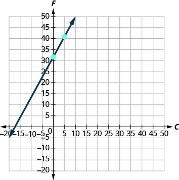
The equation \(F=\frac{9}{5}C+32\) is used to convert temperatures, \(C\), on the Celsius scale to temperatures, \(F\), on the Fahrenheit scale.

• Find the Fahrenheit temperature for a Celsius temperature of \(0\).
• Find the Fahrenheit temperature for a Celsius temperature of \(20\).
• Interpret the slope and \(F\)-intercept of the equation.
• Graph the equation.

1. \(\begin{array}{ll}{\text { Find the Fahrenheit temperature for a Celsius temperature of } 0 .} & {F=\frac{9}{5} C+32} \\ {\text { Find } F \text { when } C=0 .} & {F=\frac{9}{5}(0)+32} \\ {\text { Simplify. }} & {F=32}\end{array}\)

2. \begin{array}{ll}{\text { Find the Fahrenheit temperature for a Celsius temperature of } 20 .} & {F=\frac{9}{5} C+32} \\ {\text { Find } F \text { when } C=20 .} & {F=\frac{9}{5}(20)+32} \\ {\text { Simplify. }} & {F=36+32} \\ {\text { Simplify. }} & {F=68}\end{array}

3. Interpret the slope and \(F\)-intercept of the equation.

Even though this equation uses \(F\) and \(C\), it is still in slope–intercept form.

The slope, \(\frac{9}{5}\), means that the temperature Fahrenheit (\(F\)) increases \(9\) degrees when the temperature Celsius (\(C\)) increases \(5\) degrees.

The \(F\)-intercept means that when the temperature is \(0°\) on the Celsius scale, it is \(32°\) on the Fahrenheit scale.

4. Graph the equation.

We’ll need to use a larger scale than our usual. Start at the \(F\)-intercept \((0,32)\) then count out the rise of \(9\) and the run of \(5\) to get a second point. See Figure \(\PageIndex{3}\).

Try It \(\PageIndex{29}\)

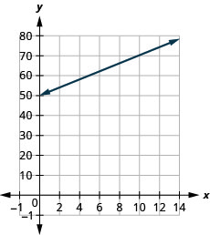
The equation \(h=2s+50\) is used to estimate a woman’s height in inches, \(h\), based on her shoe size, \(s\).

• Estimate the height of a child who wears women’s shoe size \(0\).
• Estimate the height of a woman with shoe size \(8\).
• Interpret the slope and \(h\)-intercept of the equation.
• \(50\) inches
• \(66\) inches
• The slope, \(2\), means that the height, \(h\), increases by \(2\) inches when the shoe size, \(s\), increases by \(1\). The \(h\)-intercept means that when the shoe size is \(0\), the height is \(50\) inches.

Try It \(\PageIndex{30}\)

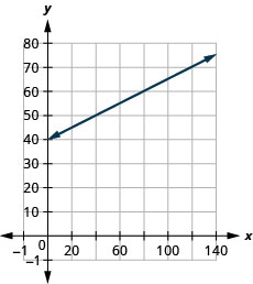
The equation \(T=\frac{1}{4}n+40\) is used to estimate the temperature in degrees Fahrenheit, \(T\), based on the number of cricket chirps, \(n\), in one minute.

• Estimate the temperature when there are no chirps.
• Estimate the temperature when the number of chirps in one minute is \(100\).
• Interpret the slope and \(T\)-intercept of the equation.
• \(40\) degrees
• \(65\) degrees
• The slope, \(\frac{1}{4}\), means that the temperature Fahrenheit (\(F\)) increases \(1\) degree when the number of chirps, \(n\), increases by \(4\). The \(T\)-intercept means that when the number of chirps is \(0\), the temperature is \(40°\).

The cost of running some types business has two components—a fixed cost and a variable cost . The fixed cost is always the same regardless of how many units are produced. This is the cost of rent, insurance, equipment, advertising, and other items that must be paid regularly. The variable cost depends on the number of units produced. It is for the material and labor needed to produce each item.

Example \(\PageIndex{31}\)

Stella has a home business selling gourmet pizzas. The equation \(C=4p+25\) models the relation between her weekly cost, \(C\), in dollars and the number of pizzas, \(p\), that she sells.

• Find Stella’s cost for a week when she sells no pizzas.
• Find the cost for a week when she sells \(15\) pizzas.
• Interpret the slope and \(C\)-intercept of the equation.

Try It \(\PageIndex{32}\)

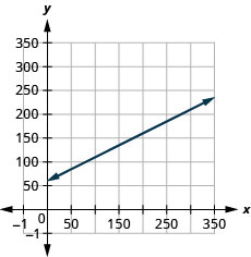
Sam drives a delivery van. The equation \(C=0.5m+60\) models the relation between his weekly cost, \(C\), in dollars and the number of miles, \(m\), that he drives.

• Find Sam’s cost for a week when he drives \(0\) miles.
• Find the cost for a week when he drives \(250\) miles.
• The slope, \(0.5\), means that the weekly cost, \(C\), increases by \($0.50 \)  when the number of miles driven, \(n\), increases by \(1\). The \(C\)-intercept means that when the number of miles driven is \(0\), the weekly cost is \($60\).

Try It \(\PageIndex{33}\)

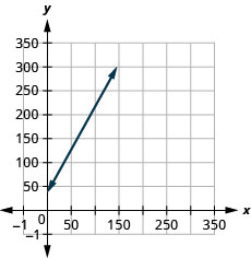
Loreen has a calligraphy business. The equation \(C=1.8n+35\) models the relation between her weekly cost, \(C\), in dollars and the number of wedding invitations, \(n\), that she writes.

• Find Loreen’s cost for a week when she writes no invitations.
• Find the cost for a week when she writes \(75\) invitations.
• The slope, \(1.8\), means that the weekly cost, \(C\), increases by \($1.80 \)  when the number of invitations, \(n\), increases by \(1\). The \(C\)-intercept means that when the number of invitations is \(0\), the weekly cost is \($35\).

Use Slopes to Identify Parallel Lines

The slope of a line indicates how steep the line is and whether it rises or falls as we read it from left to right. Two lines that have the same slope are called parallel lines. Parallel lines never intersect.

What about vertical lines? The slope of a vertical line is undefined, so vertical lines don’t fit in the definition above. We say that vertical lines that have different \(x\)-intercepts are parallel. See Figure \(\PageIndex{5}\).

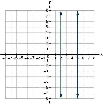
PARALLEL LINES

Parallel lines are lines in the same plane that do not intersect.

• Parallel lines have the same slope and different \(y\)-intercepts.
• If \(m_{1}\) and \(m_{2}\) are the slopes of two parallel lines then \(m_{1} = m_{2}\).
• Parallel vertical lines have different \(x\)-intercepts.

Let’s graph the equations \(y=−2x+3\) and \(2x+y=−1\) on the same grid. The first equation is already in slope–intercept form: \(y=−2x+3\). We solve the second equation for \(y\):

\[\begin{aligned} 2x+y &=-1 \\ y &=-2x-1 \end{aligned}\]

Graph the lines.

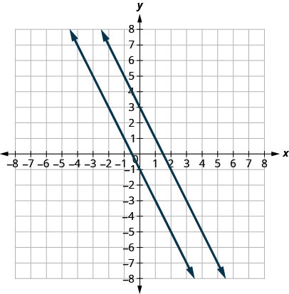
Notice the lines look parallel. What is the slope of each line? What is the \(y\)-intercept of each line?

\[\begin{array}{lll} {y} & {=m x+b} & {y=m x+b} \\ {y} & {=-2 x+3} & {y=-2 x-1} \\ {m} & {=-2} & {m=-2}\\ {b} & {=3,(0,3)} & {b=-1,(0,-1)}\end{array}\]

The slopes of the lines are the same and the \(y\)-intercept of each line is different. So we know these lines are parallel.

Since parallel lines have the same slope and different \(y\)-intercepts, we can now just look at the slope–intercept form of the equations of lines and decide if the lines are parallel.

Example \(\PageIndex{34}\)

Use slopes and \(y\)-intercepts to determine if the lines \(3x−2y=6\) and \(y = \frac{3}{2}x + 1\) are parallel.

\(\begin{array} {lrll} {\text { Solve the first equation for } y .} &{ 3 x-2 y} &{=} &{6}\\{} & {-2y} &{ =}&{-3 x+6 }\\ {} &{\frac{-2 y}{-2}}&{ =}&{\frac{-3 x+6}{-2}} \\ {} & {y }&{=}&{\frac{3}{2} x-3} \end{array}\)

The equation is now in slope–intercept form.

The equation of the second line is already in slope–intercept form.

Identify the slope and \(y\)-intercept of both lines.

\(\begin{array}{lll}{y=\frac{3}{2} x+1} & {} & {y=\frac{3}{2} x-3} \\ {y=m x+b} & {} & {y=m x+b}\\ {m=\frac{3}{2}} & {} & {m=\frac{3}{2}} \\ {y\text{-intercept is }(0, 1)} & {} & {y\text{-intercept is }(0, −3)} \end{array}\)

The lines have the same slope and different \(y\)-intercepts and so they are parallel. You may want to graph the lines to confirm whether they are parallel.

Try It \(\PageIndex{35}\)

Use slopes and \(y\)-intercepts to determine if the lines \(2x+5y=5\) and \(y=−\frac{2}{5}x−4\) are parallel.

Try It \(\PageIndex{36}\)

Use slopes and \(y\)-intercepts to determine if the lines \(4x−3y=6\) and \(y=\frac{4}{3}x−1\) are parallel.

Example \(\PageIndex{37}\)

Use slopes and \(y\)-intercepts to determine if the lines \(y=−4\) and \(y=3\) are parallel.

\(\begin{array}{llll}{\text{Write each equation in slope-intercept form.}} &{y=-4} & {\text { and }} &{ y=3} \\ {\text{Since there is no }x\text{ term we write }0x.} &{y=0 x-4} & {} &{y=0 x+3} \\ {\text{Identify the slope and }y\text{-intercept of both lines.}} &{y=m x+b} &{} & {y=m x+b} \\ {} &{m=0} &{} & {m=0} \\{} & {y\text {-intercept is }(0,4)} &{} & {y \text {-intercept is }(0,3)}\end{array}\)

The lines have the same slope and different \(y\)-intercepts and so they are parallel.

There is another way you can look at this example. If you recognize right away from the equations that these are horizontal lines, you know their slopes are both \(0\). Since the horizontal lines cross the \(y\)-axis at \(y=−4\) and at \(y=3\), we know the \(y\)-intercepts are \((0,−4)\) and \((0,3)\). The lines have the same slope and different \(y\)-intercepts and so they are parallel.

Try It \(\PageIndex{38}\)

Use slopes and \(y\)-intercepts to determine if the lines \(y=8\) and \(y=−6\) are parallel.

Try It \(\PageIndex{39}\)

Use slopes and \(y\)-intercepts to determine if the lines \(y=1\) and \(y=−5\) are parallel.

Example \(\PageIndex{40}\)

Use slopes and \(y\)-intercepts to determine if the lines \(x=−2\) and \(x=−5\) are parallel.

\[x=-2 \text { and } x=-5\]

Since there is no \(y\), the equations cannot be put in slope–intercept form. But we recognize them as equations of vertical lines. Their \(x\)-intercepts are \(−2\) and \(−5\). Since their \(x\)-intercepts are different, the vertical lines are parallel.

Try It \(\PageIndex{41}\)

Use slopes and \(y\)-intercepts to determine if the lines \(x=1\) and \(x=−5\) are parallel.

Try It \(\PageIndex{42}\)

Use slopes and \(y\)-intercepts to determine if the lines \(x=8\) and \(x=−6\) are parallel.

Example \(\PageIndex{43}\)

Use slopes and \(y\)-intercepts to determine if the lines \(y=2x−3\) and \(−6x+3y=−9\) are parallel. You may want to graph these lines, too, to see what they look like.

\(\begin{array} {llll} {\text { The first equation is already in slope-intercept form. }} & {y=2x-3}&{}&{} \\ \\ {\text { Solve the second equation for } y} & {-6x+3y} &{=}&{-9} \\{} & {3y}&{=}&{6x-9} \\ {}&{\frac{3y}{3} }&{=}&{\frac{6x-9}{3}} \\{} & {y}&{=}&{2x-3}\end{array}\)

The second equation is now in slope–intercept form as well.

\[\begin{array}{lll}{y=2x-3} &{} & {y=2x-3} \\ {y=mx+b} &{} & {y=mx+b} \\ {m=2} &{} & {m=2} \\ {\text{The }y\text{-intercept is }(0 ,−3)} &{} & {\text{The }y\text{-intercept is }(0 ,−3)} \end{array} \nonumber\]

The lines have the same slope, but they also have the same \(y\)-intercepts. Their equations represent the same line. They are not parallel; they are the same line.

Try It \(\PageIndex{44}\)

Use slopes and \(y\)-intercepts to determine if the lines \(y=−\frac{1}{2}x+1\) and \(x+2y=2\) are parallel.

not parallel; same line

Try It \(\PageIndex{45}\)

Use slopes and \(y\)-intercepts to determine if the lines \(y=\frac{3}{4}x−3\) and \(3x−4y=12\) are parallel.

Use Slopes to Identify Perpendicular Lines

Let’s look at the lines whose equations are \(y=\frac{1}{4}x−1\) and \(y=−4x+2\), shown in Figure \(\PageIndex{5}\).

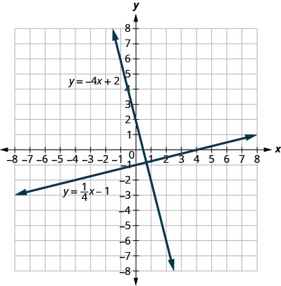
These lines lie in the same plane and intersect in right angles. We call these lines perpendicular .

What do you notice about the slopes of these two lines? As we read from left to right, the line \(y=\frac{1}{4}x−1\) rises, so its slope is positive. The line \(y=−4x+2\) drops from left to right, so it has a negative slope. Does it make sense to you that the slopes of two perpendicular lines will have opposite signs?

If we look at the slope of the first line, \(m_{1}=\frac{1}{4}\), and the slope of the second line, \(m_{2}=−4\), we can see that they are negative reciprocals of each other. If we multiply them, their product is \(−1\).

\[\begin{array}{c}{m_{1} \cdot m_{2}} \\ {\frac{1}{4}(-4)} \\ {-1}\end{array}\]

This is always true for perpendicular lines and leads us to this definition.

PERPENDICULAR LINES

Perpendicular lines are lines in the same plane that form a right angle.

If \(m_{1}\) and \(m_{2}\) are the slopes of two perpendicular lines, then:

\[m_{1} \cdot m_{2}=-1 \text { and } m_{1}=\frac{-1}{m_{2}}\]

• Vertical lines and horizontal lines are always perpendicular to each other.

We were able to look at the slope–intercept form of linear equations and determine whether or not the lines were parallel. We can do the same thing for perpendicular lines.

We find the slope–intercept form of the equation, and then see if the slopes are negative reciprocals. If the product of the slopes is \(−1\), the lines are perpendicular. Perpendicular lines may have the same \(y\)-intercepts.

Example \(\PageIndex{46}\)

Use slopes to determine if the lines, \(y=−5x−4\) and \(x−5y=5\) are perpendicular.

The first equation is already in slope–intercept form: \(\quad y=−5x−4\) \(\begin{array} {llll} {\text{Solve the second equation for }y.} &{x-5y} &{=} &{5} \\{} &{-5 y} &{=} &{-x+5} \\ {} & {\frac{-5 y}{-5}} &{=} &{\frac{-x+5}{-5}} \\ {} &{y} &{=} &{\frac{1}{5} x-1} \end{array}\)

The second equation is now in slope-intercept form as well.

\(\begin{array} {lrllllll} {\text{Identify the slope of each line.}} &{y} &{=} &{-5 x-4} & {} &{y} &{=} &{\frac{1}{5} x-1} \\ {} &{y} &{=} &{m x+b} & {} &{y} &{=} &{m x+b}\\ {} &{m_{1}} &{=}&{-5} & {} &{m_{2}} &{=}&{\frac{1}{5}}\end{array}\)

The slopes are negative reciprocals of each other, so the lines are perpendicular. We check by multiplying the slopes,

\[\begin{array}{l}{m_{1} \cdot m_{2}} \\ {-5\left(\frac{1}{5}\right)} \\ {-1\checkmark}\end{array}\]

Try It \(\PageIndex{47}\)

Use slopes to determine if the lines \(y=−3x+2\) and \(x−3y=4\) are perpendicular.

perpendicular

Try It \(\PageIndex{48}\)

Use slopes to determine if the lines \(y=2x−5\) and \(x+2y=−6\) are perpendicular.

Example \(\PageIndex{49}\)

Use slopes to determine if the lines, \(7x+2y=3\) and \(2x+7y=5\) are perpendicular.

\(\begin{array}{lrlrl}{\text{Solve the equations for y.}} &{7 x+2 y} & {=3} & {2 x+7 y}&{=}&{5} \\{} & {2 y} & {=-7 x+3} & {7 y}&{=}&{-2 x+5} \\ {} &{\frac{2 y}{2}} & {=\frac{-7 x+3}{2} \quad} & {\frac{7 y}{7}}&{=}&{\frac{-2 x+5}{7}} \\ {} &{y} & {=-\frac{7}{2} x+\frac{3}{2}} &{y}&{=}&{\frac{-2}{7}x + \frac{5}{7}}\\ \\{\text{Identify the slope of each line.}} & {y}&{=m x+b} &{y}&{=}&{m x+b} \\{} & {m_{1}} & {=-\frac{7}{2} }&{ m_{2}}&{=}&{-\frac{2}{7}}\end{array}\)

The slopes are reciprocals of each other, but they have the same sign. Since they are not negative reciprocals, the lines are not perpendicular.

Try It \(\PageIndex{50}\)

Use slopes to determine if the lines \(5x+4y=1\) and \(4x+5y=3\) are perpendicular.

not perpendicular

Try It \(\PageIndex{51}\)

Use slopes to determine if the lines \(2x−9y=3\) and \(9x−2y=1\) are perpendicular.

Access this online resource for additional instruction and practice with graphs.

• Explore the Relation Between a Graph and the Slope–Intercept Form of an Equation of a Line

Key Concepts

• The slope–intercept form of an equation of a line with slope mm and \(y\)-intercept, \((0,b)\) is, \(y=mx+b\).
• Use the slope formula \(m = \dfrac{\text{rise}}{\text{run}}\) to identify the rise and the run.
• If it only has one variable, it is a vertical or horizontal line. \(x = a\) is a vertical line passing through the \(x\)-axis at a. \(y = b\) is a horizontal line passing through the \(y\)-axis at \(b\).
• If \(y\) is isolated on one side of the equation, in the form \(y=mx+b\), graph by using the slope and \(y\)-intercept. Identify the slope and \(y\)-intercept and then graph.
• If the equation is of the form \(Ax+By=C\), find the intercepts. Find the \(x\)- and \(y\)-intercepts, a third point, and then graph.
• If \(m_1\) and \(m_2\) are the slopes of two parallel lines then \(m_1 = m_2\).
• If \(m_1\) and \(m_2\) are the slopes of two perpendicular lines, then \(m_1\cdot m_2=−1\) and \(m_1=\frac{−1}{m_2}\).

If you're seeing this message, it means we're having trouble loading external resources on our website.

If you're behind a web filter, please make sure that the domains *.kastatic.org and *.kasandbox.org are unblocked.

To log in and use all the features of Khan Academy, please enable JavaScript in your browser.

Unit 3: Linear relationships

Lesson 3: representing proportional relationships.

• Graphing proportional relationships: unit rate (Opens a modal)
• Graphing proportional relationships from a table (Opens a modal)
• Graphing proportional relationships from an equation (Opens a modal)
• Graphing proportional relationships Get 3 of 4 questions to level up!

Lesson 4: Comparing proportional relationships

• Rates & proportional relationships example (Opens a modal)
• Rates & proportional relationships: gas mileage (Opens a modal)
• Rates & proportional relationships Get 5 of 7 questions to level up!

Lesson 7: Representations of linear relationships

• Linear & nonlinear functions: missing value (Opens a modal)

Lesson 8: Translating to y=mx+b

• Intro to slope-intercept form (Opens a modal)
• Graph from slope-intercept equation (Opens a modal)

Lesson 9: Slopes don't have to be positive

• Intro to intercepts (Opens a modal)
• Slope-intercept equation from slope & point (Opens a modal)
• Linear & nonlinear functions: word problem (Opens a modal)
• Intercepts from a graph Get 3 of 4 questions to level up!
• Slope from graph Get 3 of 4 questions to level up!
• Slope-intercept intro Get 3 of 4 questions to level up!
• Graph from slope-intercept form Get 3 of 4 questions to level up!
• Slope-intercept equation from graph Get 3 of 4 questions to level up!

Lesson 10: Calculating slope

• No videos or articles available in this lesson
• Slope from two points Get 3 of 4 questions to level up!

Lesson 11: Equations of all kinds of lines

• Converting to slope-intercept form (Opens a modal)

Extra practice: Slope

• Intro to slope (Opens a modal)
• Worked examples: slope-intercept intro (Opens a modal)
• Graphing slope-intercept form (Opens a modal)
• Writing slope-intercept equations (Opens a modal)
• Slope-intercept form review (Opens a modal)
• Slope-intercept from two points Get 3 of 4 questions to level up!

Lesson 12: Solutions to linear equations

• Solutions to 2-variable equations (Opens a modal)
• Worked example: solutions to 2-variable equations (Opens a modal)
• Solutions to 2-variable equations Get 3 of 4 questions to level up!

Lesson 13: More solutions to linear equations

• Completing solutions to 2-variable equations (Opens a modal)
• Complete solutions to 2-variable equations Get 3 of 4 questions to level up!

Extra practice: Intercepts

• x-intercept of a line (Opens a modal)
• Intercepts from an equation (Opens a modal)
• Worked example: intercepts from an equation (Opens a modal)
• Intercepts of lines review (x-intercepts and y-intercepts) (Opens a modal)
• Intercepts from an equation Get 3 of 4 questions to level up!