hypothesis testing z value

Z-Test for Statistical Hypothesis Testing Explained

The Z-test is a statistical hypothesis test used to determine where the distribution of the test statistic we are measuring, like the mean , is part of the normal distribution .

There are multiple types of Z-tests, however, we’ll focus on the easiest and most well known one, the one sample mean test. This is used to determine if the difference between the mean of a sample and the mean of a population is statistically significant.

What Is a Z-Test?

A Z-test is a type of statistical hypothesis test where the test-statistic follows a normal distribution.  

The name Z-test comes from the Z-score of the normal distribution. This is a measure of how many standard deviations away a raw score or sample statistics is from the populations’ mean.

Z-tests are the most common statistical tests conducted in fields such as healthcare and data science . Therefore, it’s an essential concept to understand.

Requirements for a Z-Test

In order to conduct a Z-test, your statistics need to meet a few requirements, including:

• A Sample size that’s greater than 30. This is because we want to ensure our sample mean comes from a distribution that is normal. As stated by the c entral limit theorem , any distribution can be approximated as normally distributed if it contains more than 30 data points.
• The standard deviation and mean of the population is known .
• The sample data is collected/acquired randomly .

More on Data Science:   What Is Bootstrapping Statistics?

Z-Test Steps

There are four steps to complete a Z-test. Let’s examine each one.

4 Steps to a Z-Test

• State the null hypothesis.
• State the alternate hypothesis.
• Choose your critical value.
• Calculate your Z-test statistics. 

1. State the Null Hypothesis

The first step in a Z-test is to state the null hypothesis, H_0 . This what you believe to be true from the population, which could be the mean of the population, μ_0 :

2. State the Alternate Hypothesis

Next, state the alternate hypothesis, H_1 . This is what you observe from your sample. If the sample mean is different from the population’s mean, then we say the mean is not equal to μ_0:

3. Choose Your Critical Value

Then, choose your critical value, α , which determines whether you accept or reject the null hypothesis. Typically for a Z-test we would use a statistical significance of 5 percent which is z = +/- 1.96 standard deviations from the population’s mean in the normal distribution:

This critical value is based on confidence intervals.

4. Calculate Your Z-Test Statistic

Compute the Z-test Statistic using the sample mean, μ_1 , the population mean, μ_0 , the number of data points in the sample, n and the population’s standard deviation, σ :

If the test statistic is greater (or lower depending on the test we are conducting) than the critical value, then the alternate hypothesis is true because the sample’s mean is statistically significant enough from the population mean.

Another way to think about this is if the sample mean is so far away from the population mean, the alternate hypothesis has to be true or the sample is a complete anomaly.

More on Data Science: Basic Probability Theory and Statistics Terms to Know

Z-Test Example

Let’s go through an example to fully understand the one-sample mean Z-test.

A school says that its pupils are, on average, smarter than other schools. It takes a sample of 50 students whose average IQ measures to be 110. The population, or the rest of the schools, has an average IQ of 100 and standard deviation of 20. Is the school’s claim correct?

The null and alternate hypotheses are:

Where we are saying that our sample, the school, has a higher mean IQ than the population mean.

Now, this is what’s called a right-sided, one-tailed test as our sample mean is greater than the population’s mean. So, choosing a critical value of 5 percent, which equals a Z-score of 1.96 , we can only reject the null hypothesis if our Z-test statistic is greater than 1.96.

If the school claimed its students’ IQs were an average of 90, then we would use a left-tailed test, as shown in the figure above. We would then only reject the null hypothesis if our Z-test statistic is less than -1.96.

Computing our Z-test statistic, we see:

Therefore, we have sufficient evidence to reject the null hypothesis, and the school’s claim is right.

Hope you enjoyed this article on Z-tests. In this post, we only addressed the most simple case, the one-sample mean test. However, there are other types of tests, but they all follow the same process just with some small nuances.  

Built In’s expert contributor network publishes thoughtful, solutions-oriented stories written by innovative tech professionals. It is the tech industry’s definitive destination for sharing compelling, first-person accounts of problem-solving on the road to innovation.

Great Companies Need Great People. That's Where We Come In.

10 Chapter 10: Hypothesis Testing with Z

Setting up the hypotheses.

When setting up the hypotheses with z, the parameter is associated with a sample mean (in the previous chapter examples the parameters for the null used 0). Using z is an occasion in which the null hypothesis is a value other than 0. For example, if we are working with mothers in the U.S. whose children are at risk of low birth weight, we can use 7.47 pounds, the average birth weight in the US, as our null value and test for differences against that. For now, we will focus on testing a value of a single mean against what we expect from the population.

Using birthweight as an example, our null hypothesis takes the form: H 0 : μ = 7.47 Notice that we are testing the value for μ, the population parameter, NOT the sample statistic ̅X (or M). We are referring to the data right now in raw form (we have not standardized it using z yet). Again, using inferential statistics, we are interested in understanding the population, drawing from our sample observations. For the research question, we have a mean value from the sample to use, we have specific data is – it is observed and used as a comparison for a set point.

As mentioned earlier, the alternative hypothesis is simply the reverse of the null hypothesis, and there are three options, depending on where we expect the difference to lie. We will set the criteria for rejecting the null hypothesis based on the directionality (greater than, less than, or not equal to) of the alternative.

If we expect our obtained sample mean to be above or below the null hypothesis value (knowing which direction), we set a directional hypothesis. O ur alternative hypothesis takes the form based on the research question itself. In our example with birthweight, this could be presented as H A : μ > 7.47 or H A : μ < 7.47. 

Note that we should only use a directional hypothesis if we have a good reason, based on prior observations or research, to suspect a particular direction. When we do not know the direction, such as when we are entering a new area of research, we use a non-directional alternative hypothesis. In our birthweight example, this could be set as H A : μ ≠ 7.47

In working with data for this course we will need to set a critical value of the test statistic for alpha (α) for use of test statistic tables in the back of the book. This is determining the critical rejection region that has a set critical value based on α.

Determining Critical Value from α

We set alpha (α) before collecting data in order to determine whether or not we should reject the null hypothesis. We set this value beforehand to avoid biasing ourselves by viewing our results and then determining what criteria we should use.

When a research hypothesis predicts an effect but does not predict a direction for the effect, it is called a non-directional hypothesis . To test the significance of a non-directional hypothesis, we have to consider the possibility that the sample could be extreme at either tail of the comparison distribution. We call this a two-tailed test .

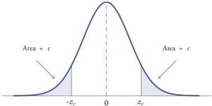
Figure 1. showing a 2-tail test for non-directional hypothesis for z for area C is the critical rejection region.

When a research hypothesis predicts a direction for the effect, it is called a directional hypothesis . To test the significance of a directional hypothesis, we have to consider the possibility that the sample could be extreme at one-tail of the comparison distribution. We call this a one-tailed test .

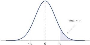
Figure 2. showing a 1-tail test for a directional hypothesis (predicting an increase) for z for area C is the critical rejection region.

Determining Cutoff Scores with Two-Tailed Tests

Typically we specify an α level before analyzing the data. If the data analysis results in a probability value below the α level, then the null hypothesis is rejected; if it is not, then the null hypothesis is not rejected. In other words, if our data produce values that meet or exceed this threshold, then we have sufficient evidence to reject the null hypothesis ; if not, we fail to reject the null (we never “accept” the null). According to this perspective, if a result is significant, then it does not matter how significant it is. Moreover, if it is not significant, then it does not matter how close to being significant it is. Therefore, if the 0.05 level is being used, then probability values of 0.049 and 0.001 are treated identically. Similarly, probability values of 0.06 and 0.34 are treated identically. Note we will discuss ways to address effect size (which is related to this challenge of NHST).

When setting the probability value, there is a special complication in a two-tailed test. We have to divide the significance percentage between the two tails. For example, with a 5% significance level, we reject the null hypothesis only if the sample is so extreme that it is in either the top 2.5% or the bottom 2.5% of the comparison distribution. This keeps the overall level of significance at a total of 5%. A one-tailed test does have such an extreme value but with a one-tailed test only one side of the distribution is considered.

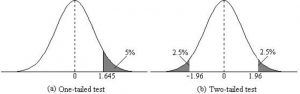
Figure 3. Critical value differences in one and two-tail tests. Photo Credit

Let’s re view th e set critical values for Z.

We discussed z-scores and probability in chapter 8.  If we revisit the z-score for 5% and 1%, we can identify the critical regions for the critical rejection areas from the unit standard normal table.

• A two-tailed test at the 5% level has a critical boundary Z score of +1.96 and -1.96
• A one-tailed test at the 5% level has a critical boundary Z score of +1.64 or -1.64
• A two-tailed test at the 1% level has a critical boundary Z score of +2.58 and -2.58
• A one-tailed test at the 1% level has a critical boundary Z score of +2.33 or -2.33.

Review: Critical values, p-values, and significance level

There are two criteria we use to assess whether our data meet the thresholds established by our chosen significance level, and they both have to do with our discussions of probability and distributions. Recall that probability refers to the likelihood of an event, given some situation or set of conditions. In hypothesis testing, that situation is the assumption that the null hypothesis value is the correct value, or that there is no effec t. The value laid out in H 0 is our condition under which we interpret our results. To reject this assumption, and thereby reject the null hypothesis, we need results that would be very unlikely if the null was true.

Now recall that values of z which fall in the tails of the standard normal distribution represent unlikely values. That is, the proportion of the area under the curve as or more extreme than z is very small as we get into the tails of the distribution. Our significance level corresponds to the area under the tail that is exactly equal to α: if we use our normal criterion of α = .05, then 5% of the area under the curve becomes what we call the rejection region (also called the critical region) of the distribution. This is illustrated in Figure 4.

Figure 4: The rejection region for a one-tailed test

The shaded rejection region takes us 5% of the area under the curve. Any result which falls in that region is sufficient evidence to reject the null hypothesis.

The rejection region is bounded by a specific z-value, as is any area under the curve. In hypothesis testing, the value corresponding to a specific rejection region is called the critical value, z crit (“z-crit”) or z* (hence the other name “critical region”). Finding the critical value works exactly the same as finding the z-score corresponding to any area under the curve like we did in Unit 1. If we go to the normal table, we will find that the z-score corresponding to 5% of the area under the curve is equal to 1.645 (z = 1.64 corresponds to 0.0405 and z = 1.65 corresponds to 0.0495, so .05 is exactly in between them) if we go to the right and -1.645 if we go to the left. The direction must be determined by your alternative hypothesis, and drawing then shading the distribution is helpful for keeping directionality straight.

Suppose, however, that we want to do a non-directional test. We need to put the critical region in both tails, but we don’t want to increase the overall size of the rejection region (for reasons we will see later). To do this, we simply split it in half so that an equal proportion of the area under the curve falls in each tail’s rejection region. For α = .05, this means 2.5% of the area is in each tail, which, based on the z-table, corresponds to critical values of z* = ±1.96. This is shown in Figure 5.

Figure 5: Two-tailed rejection region

Thus, any z-score falling outside ±1.96 (greater than 1.96 in absolute value) falls in the rejection region. When we use z-scores in this way, the obtained value of z (sometimes called z-obtained) is something known as a test statistic, which is simply an inferential statistic used to test a null hypothesis.

Calculate the test statistic: Z

Now that we understand setting up the hypothesis and determining the outcome, let’s examine hypothesis testing with z!  The next step is to carry out the study and get the actual results for our sample. Central to hypothesis test is comparison of the population and sample means. To make our calculation and determine where the sample is in the hypothesized distribution we calculate the Z for the sample data.

Make a decision

To decide whether to reject the null hypothesis, we compare our sample’s Z score to the Z score that marks our critical boundary. If our sample Z score falls inside the rejection region of the comparison distribution (is greater than the z-score critical boundary) we reject the null hypothesis.

The formula for our z- statistic has not changed:

To formally test our hypothesis, we compare our obtained z-statistic to our critical z-value. If z obt > z crit , that means it falls in the rejection region (to see why, draw a line for z = 2.5 on Figure 1 or Figure 2) and so we reject H 0 . If z obt < z crit , we fail to reject. Remember that as z gets larger, the corresponding area under the curve beyond z gets smaller. Thus, the proportion, or p-value, will be smaller than the area for α, and if the area is smaller, the probability gets smaller. Specifically, the probability of obtaining that result, or a more extreme result, under the condition that the null hypothesis is true gets smaller.

Conversely, if we fail to reject, we know that the proportion will be larger than α because the z-statistic will not be as far into the tail. This is illustrated for a one- tailed test in Figure 6.

Figure 6. Relation between α, z obt , and p

When the null hypothesis is rejected, the effect is said to be statistically significant . Do not confuse statistical significance with practical significance. A small effect can be highly significant if the sample size is large enough.

Why does the word “significant” in the phrase “statistically significant” mean something so different from other uses of the word? Interestingly, this is because the meaning of “significant” in everyday language has changed. It turns out that when the procedures for hypothesis testing were developed, something was “significant” if it signified something. Thus, finding that an effect is statistically significant signifies that the effect is real and not due to chance. Over the years, the meaning of “significant” changed, leading to the potential misinterpretation.

Review: Steps of the Hypothesis Testing Process

The process of testing hypotheses follows a simple four-step procedure. This process will be what we use for the remained of the textbook and course, and though the hypothesis and statistics we use will change, this process will not.

Step 1: State the Hypotheses

Your hypotheses are the first thing you need to lay out. Otherwise, there is nothing to test! You have to state the null hypothesis (which is what we test) and the alternative hypothesis (which is what we expect). These should be stated mathematically as they were presented above AND in words, explaining in normal English what each one means in terms of the research question.

Step 2: Find the Critical Values

Next, we formally lay out the criteria we will use to test our hypotheses. There are two pieces of information that inform our critical values: α, which determines how much of the area under the curve composes our rejection region, and the directionality of the test, which determines where the region will be.

Step 3: Compute the Test Statistic

Once we have our hypotheses and the standards we use to test them, we can collect data and calculate our test statistic, in this case z . This step is where the vast majority of differences in future chapters will arise: different tests used for different data are calculated in different ways, but the way we use and interpret them remains the same.

Step 4: Make the Decision

Finally, once we have our obtained test statistic, we can compare it to our critical value and decide whether we should reject or fail to reject the null hypothesis. When we do this, we must interpret the decision in relation to our research question, stating what we concluded, what we based our conclusion on, and the specific statistics we obtained.

Example: Movie Popcorn

Let’s see how hypothesis testing works in action by working through an example. Say that a movie theater owner likes to keep a very close eye on how much popcorn goes into each bag sold, so he knows that the average bag has 8 cups of popcorn and that this varies a little bit, about half a cup. That is, the known population mean is μ = 8.00 and the known population standard deviation is σ =0.50. The owner wants to make sure that the newest employee is filling bags correctly, so over the course of a week he randomly assesses 25 bags filled by the employee to test for a difference (n = 25). He doesn’t want bags overfilled or under filled, so he looks for differences in both directions. This scenario has all of the information we need to begin our hypothesis testing procedure.

Our manager is looking for a difference in the mean cups of popcorn bags compared to the population mean of 8. We will need both a null and an alternative hypothesis written both mathematically and in words. We’ll always start with the null hypothesis:

H 0 : There is no difference in the cups of popcorn bags from this employee H 0 : μ = 8.00

Notice that we phrase the hypothesis in terms of the population parameter μ, which in this case would be the true average cups of bags filled by the new employee.

Our assumption of no difference, the null hypothesis, is that this mean is exactly

the same as the known population mean value we want it to match, 8.00. Now let’s do the alternative:

H A : There is a difference in the cups of popcorn bags from this employee H A : μ ≠ 8.00

In this case, we don’t know if the bags will be too full or not full enough, so we do a two-tailed alternative hypothesis that there is a difference.

Our critical values are based on two things: the directionality of the test and the level of significance. We decided in step 1 that a two-tailed test is the appropriate directionality. We were given no information about the level of significance, so we assume that α = 0.05 is what we will use. As stated earlier in the chapter, the critical values for a two-tailed z-test at α = 0.05 are z* = ±1.96. This will be the criteria we use to test our hypothesis. We can now draw out our distribution so we can visualize the rejection region and make sure it makes sense

Figure 7: Rejection region for z* = ±1.96

Step 3: Calculate the Test Statistic

Now we come to our formal calculations. Let’s say that the manager collects data and finds that the average cups of this employee’s popcorn bags is ̅X = 7.75 cups. We can now plug this value, along with the values presented in the original problem, into our equation for z:

So our test statistic is z = -2.50, which we can draw onto our rejection region distribution:

Figure 8: Test statistic location

Looking at Figure 5, we can see that our obtained z-statistic falls in the rejection region. We can also directly compare it to our critical value: in terms of absolute value, -2.50 > -1.96, so we reject the null hypothesis. We can now write our conclusion:

When we write our conclusion, we write out the words to communicate what it actually means, but we also include the average sample size we calculated (the exact location doesn’t matter, just somewhere that flows naturally and makes sense) and the z-statistic and p-value. We don’t know the exact p-value, but we do know that because we rejected the null, it must be less than α.

Effect Size

When we reject the null hypothesis, we are stating that the difference we found was statistically significant, but we have mentioned several times that this tells us nothing about practical significance. To get an idea of the actual size of what we found, we can compute a new statistic called an effect size. Effect sizes give us an idea of how large, important, or meaningful a statistically significant effect is.

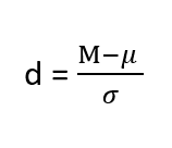
For mean differences like we calculated here, our effect size is Cohen’s d :

Effect sizes are incredibly useful and provide important information and clarification that overcomes some of the weakness of hypothesis testing. Whenever you find a significant result, you should always calculate an effect size

Table 1. Interpretation of Cohen’s d

Example: Office Temperature

Let’s do another example to solidify our understanding. Let’s say that the office building you work in is supposed to be kept at 74 degree Fahrenheit but is allowed

to vary by 1 degree in either direction. You suspect that, as a cost saving measure, the temperature was secretly set higher. You set up a formal way to test your hypothesis.

You start by laying out the null hypothesis:

H 0 : There is no difference in the average building temperature H 0 : μ = 74

Next you state the alternative hypothesis. You have reason to suspect a specific direction of change, so you make a one-tailed test:

H A : The average building temperature is higher than claimed H A : μ > 74

Now that you have everything set up, you spend one week collecting temperature data:

You calculate the average of these scores to be 𝑋̅ = 76.6 degrees. You use this to calculate the test statistic, using μ = 74 (the supposed average temperature), σ = 1.00 (how much the temperature should vary), and n = 5 (how many data points you collected):

z = 76.60 − 74.00 = 2.60    = 5.78

          1.00/√5            0.45

This value falls so far into the tail that it cannot even be plotted on the distribution!

Figure 7: Obtained z-statistic

You compare your obtained z-statistic, z = 5.77, to the critical value, z* = 1.645, and find that z > z*. Therefore you reject the null hypothesis, concluding: Based on 5 observations, the average temperature (𝑋̅ = 76.6 degrees) is statistically significantly higher than it is supposed to be, z = 5.77, p < .05.

d = (76.60-74.00)/ 1= 2.60

The effect size you calculate is definitely large, meaning someone has some explaining to do!

Example: Different Significance Level

First, let’s take a look at an example phrased in generic terms, rather than in the context of a specific research question, to see the individual pieces one more time. This time, however, we will use a stricter significance level, α = 0.01, to test the hypothesis.

We will use 60 as an arbitrary null hypothesis value: H 0 : The average score does not differ from the population H 0 : μ = 50

We will assume a two-tailed test: H A : The average score does differ H A : μ ≠ 50

We have seen the critical values for z-tests at α = 0.05 levels of significance several times. To find the values for α = 0.01, we will go to the standard normal table and find the z-score cutting of 0.005 (0.01 divided by 2 for a two-tailed test) of the area in the tail, which is z crit * = ±2.575. Notice that this cutoff is much higher than it was for α = 0.05. This is because we need much less of the area in the tail, so we need to go very far out to find the cutoff. As a result, this will require a much larger effect or much larger sample size in order to reject the null hypothesis.

We can now calculate our test statistic.  The average of 10 scores is M = 60.40 with a µ = 60. We will use σ = 10 as our known population standard deviation. From this information, we calculate our z-statistic as:

Our obtained z-statistic, z = 0.13, is very small. It is much less than our critical value of 2.575. Thus, this time, we fail to reject the null hypothesis. Our conclusion would look something like:

Notice two things about the end of the conclusion. First, we wrote that p is greater than instead of p is less than, like we did in the previous two examples. This is because we failed to reject the null hypothesis. We don’t know exactly what the p- value is, but we know it must be larger than the α level we used to test our hypothesis. Second, we used 0.01 instead of the usual 0.05, because this time we tested at a different level. The number you compare to the p-value should always be the significance level you test at. Because we did not detect a statistically significant effect, we do not need to calculate an effect size. Note: some statisticians will suggest to always calculate effects size as a possibility of Type II error. Although insignificant, calculating d = (60.4-60)/10 = .04 which suggests no effect (and not a possibility of Type II error).

Review Considerations in Hypothesis Testing

Errors in hypothesis testing.

Keep in mind that rejecting the null hypothesis is not an all-or-nothing decision. The Type I error rate is affected by the α level: the lower the α level the lower the Type I error rate. It might seem that α is the probability of a Type I error. However, this is not correct. Instead, α is the probability of a Type I error given that the null hypothesis is true. If the null hypothesis is false, then it is impossible to make a Type I error. The second type of error that can be made in significance testing is failing to reject a false null hypothesis. This kind of error is called a Type II error.

Statistical Power

The statistical power of a research design is the probability of rejecting the null hypothesis given the sample size and expected relationship strength. Statistical power is the complement of the probability of committing a Type II error. Clearly, researchers should be interested in the power of their research designs if they want to avoid making Type II errors. In particular, they should make sure their research design has adequate power before collecting data. A common guideline is that a power of .80 is adequate. This means that there is an 80% chance of rejecting the null hypothesis for the expected relationship strength.

Given that statistical power depends primarily on relationship strength and sample size, there are essentially two steps you can take to increase statistical power: increase the strength of the relationship or increase the sample size. Increasing the strength of the relationship can sometimes be accomplished by using a stronger manipulation or by more carefully controlling extraneous variables to reduce the amount of noise in the data (e.g., by using a within-subjects design rather than a between-subjects design). The usual strategy, however, is to increase the sample size. For any expected relationship strength, there will always be some sample large enough to achieve adequate power.

Inferential statistics uses data from a sample of individuals to reach conclusions about the whole population. The degree to which our inferences are valid depends upon how we selected the sample (sampling technique) and the characteristics (parameters) of population data. Statistical analyses assume that sample(s) and population(s) meet certain conditions called statistical assumptions.

It is easy to check assumptions when using statistical software and it is important as a researcher to check for violations; if violations of statistical assumptions are not appropriately addressed then results may be interpreted incorrectly.

Learning Objectives

Having read the chapter, students should be able to:

• Conduct a hypothesis test using a z-score statistics, locating critical region, and make a statistical decision including.
• Explain the purpose of measuring effect size and power, and be able to compute Cohen’s d.

Exercises – Ch. 10

• List the main steps for hypothesis testing with the z-statistic. When and why do you calculate an effect size?
• z = 1.99, two-tailed test at α = 0.05
• z = 1.99, two-tailed test at α = 0.01
• z = 1.99, one-tailed test at α = 0.05
• You are part of a trivia team and have tracked your team’s performance since you started playing, so you know that your scores are normally distributed with μ = 78 and σ = 12. Recently, a new person joined the team, and you think the scores have gotten better. Use hypothesis testing to see if the average score has improved based on the following 8 weeks’ worth of score data: 82, 74, 62, 68, 79, 94, 90, 81, 80.
• A study examines self-esteem and depression in teenagers.  A sample of 25 teens with a low self-esteem are given the Beck Depression Inventory.  The average score for the group is 20.9.  For the general population, the average score is 18.3 with σ = 12.  Use a two-tail test with α = 0.05 to examine whether teenagers with low self-esteem show significant differences in depression.
• You get hired as a server at a local restaurant, and the manager tells you that servers’ tips are $42 on average but vary about $12 (μ = 42, σ = 12). You decide to track your tips to see if you make a different amount, but because this is your first job as a server, you don’t know if you will make more or less in tips. After working 16 shifts, you find that your average nightly amount is $44.50 from tips. Test for a difference between this value and the population mean at the α = 0.05 level of significance.

Answers to Odd- Numbered Exercises – Ch. 10

1. List hypotheses. Determine critical region. Calculate z.  Compare z to critical region. Draw Conclusion.  We calculate an effect size when we find a statistically significant result to see if our result is practically meaningful or important

5. Step 1: H 0 : μ = 42 “My average tips does not differ from other servers”, H A : μ ≠ 42 “My average tips do differ from others”

Introduction to Statistics for Psychology Copyright © 2021 by Alisa Beyer is licensed under a Creative Commons Attribution-NonCommercial-ShareAlike 4.0 International License , except where otherwise noted.

Share This Book

Z-Score: Definition, Formula, Calculation & Interpretation

Saul Mcleod, PhD

Editor-in-Chief for Simply Psychology

BSc (Hons) Psychology, MRes, PhD, University of Manchester

Saul Mcleod, PhD., is a qualified psychology teacher with over 18 years of experience in further and higher education. He has been published in peer-reviewed journals, including the Journal of Clinical Psychology.

Learn about our Editorial Process

Olivia Guy-Evans, MSc

Associate Editor for Simply Psychology

BSc (Hons) Psychology, MSc Psychology of Education

Olivia Guy-Evans is a writer and associate editor for Simply Psychology. She has previously worked in healthcare and educational sectors.

On This Page:

A z-score is a statistical measure that describes the position of a raw score in terms of its distance from the mean, measured in standard deviation units. A positive z-score indicates that the value lies above the mean, while a negative z-score indicates that the value lies below the mean.

It is also known as a standard score because it allows scores on different variables to be compared by standardizing the distribution. A standard normal distribution (SND) is a normally shaped distribution with a mean of 0 and a standard deviation (SD) of 1 (see Fig. 1).

Why Are Z-Scores Important?

It is useful to standardize the values (raw scores) of a  normal distribution  by converting them into z-scores because:

• Probability estimation : Z-scores can be used to estimate the probability of a particular data point occurring within a normal distribution. By converting z-scores to percentiles or using a standard normal distribution table, you can determine the likelihood of a value being above or below a certain threshold.
• Hypothesis testing : Z-scores are used in hypothesis testing to determine the significance of results. By comparing the z-score of a sample statistic to critical values, you can decide whether to reject or fail to reject a null hypothesis.
• Comparing datasets : Z-scores allow you to compare data points from different datasets by standardizing the values. This is useful when the datasets have different scales or units.
• Identifying outliers : Z-scores help identify outliers, which are data points significantly different from the rest of the dataset. Typically, data points with z-scores greater than 3 or less than -3 are considered potential outliers and may warrant further investigation.

How To Calculate

The formula for calculating a z-score is z = (x-μ)/σ, where x is the raw score, μ is the population mean, and σ is the population standard deviation.

As the formula shows, the z-score is simply the raw score minus the population mean, divided by the population standard deviation.

When the population mean and the population standard deviation are unknown, the standard score may be calculated using the sample mean (x̄) and sample standard deviation (s) as estimates of the population values.

To calculate a z-score, follow these steps:

• Identify the individual score ( x ) you want to convert to a z-score.
• Determine the mean ( μ or mu ) of the dataset. The mean is the average of all the scores.
• Calculate the standard deviation ( σ or sigma ) of the dataset. The standard deviation measures how spread out the scores are from the mean.
• Subtract the mean ( μ ) from the individual score ( x ). This will give you the difference between the score and the mean.
• Divide the difference you calculated in step 4 by the standard deviation ( σ ). The result is the z-score.

Interpretation

The value of the z-score tells you how many standard deviations you are away from the mean. A larger absolute value indicates a greater distance from the mean.

• Positive z-score : If a z-score is positive, it indicates that the data point is above the mean. For example, a z-score of 1.5 means the data point is 1.5 standard deviations above the mean.
• Negative z-score : If a z-score is negative, it indicates that the data point is below the mean. For example, a z-score of -2 means the data point is 2 standard deviations below the mean.
• Zero z-score : A z-score of zero indicates that the data point is equal to the mean.

Another way to interpret z-scores is by creating a standard normal distribution, also known as the z-score distribution, or probability distribution (see Fig. 3).

Probability Estimation

When working with z-scores, the data is assumed to follow a standard normal distribution with a mean of 0 and a standard deviation of 1. This allows for the use of standard normal distribution tables or calculators to determine probabilities.

The z-score tells us how many standard deviations a data point is from the mean. Once we know the z-score, we can estimate the probability of a data point falling within a specific range or being above or below a certain value.

In a standard normal distribution, there’s a handy rule called the empirical rule, or the 68-95-99.7 rule. This rule states that:

• Approximately 68% of the data falls within one standard deviation of the mean (z-scores between -1 and 1).
• Around 95% of the data falls within two standard deviations of the mean (z-scores between -2 and 2).
• Nearly 99.7% of the data falls within three standard deviations of the mean (z-scores between -3 and 3).

Figure 3 shows the proportion of a standard normal distribution in percentages. As you can see, there’s a 95% probability of randomly selecting a score between -1.96 and +1.96 standard deviations from the mean.

Using the standard normal distribution, researchers can calculate the probability of randomly obtaining a score from the sample. For example, there’s a 68% chance of randomly selecting a score between -1 and +1 standard deviations from the mean.

Hypothesis Testing

Using a z-score table lets you quickly determine the probability associated with a specific value in a dataset, helping you make decisions and draw conclusions based on your data.

• If you have a one-tailed test, you will look for the area to the left (for a left-tailed test) or right (for a right-tailed test) of your z-score.
• If you have a two-tailed test, you will look for the area in both tails combined.

The significance level (α) is the probability threshold for rejecting the null hypothesis. Common significance levels are 0.01, 0.05, and 0.10. The critical values are the z-scores that correspond to the chosen significance level. These values can be found using a standard normal distribution table or calculator.

A Z-score table shows the percentage of values (usually a decimal figure) to the left of a given Z-score on a standard normal distribution.

1. Identify the parts of the z-score :

• The z-score consists of a whole number and decimal parts
• For example, if your z-score is 1.24, the whole number part is 1, and the decimal part is 0.24

2. Find the corresponding probability in the z-score table :

• Z-score tables are usually organized with the whole number part of the z-score in the leftmost column and the decimal part across the top row
• Locate the whole number part of your z-score in the leftmost column
• Move across the row until you find the column that matches the decimal part of your z-score
• The value at the intersection of the row and column is the probability (area under the curve) associated with your z-score

3. Interpret the probability :

• For a left-tailed test, the probability you found in the table is your p-value
• For a right-tailed test, subtract the probability you found from 1 to get your p-value
• For a two-tailed test, if your z-score is positive, double the probability you found to get your p-value; if your z-score is negative, subtract the probability from 1 and then double the result to get your p-value
• Compare the probability to your chosen alpha level (0.05 or 0.01). If the probability is less than the alpha level, the result is considered statistically significant

In statistical analysis, if there is less than a 5% chance of randomly selecting a particular raw score, it is considered a statistically significant result. This means the result is unlikely to have occurred by chance alone and is more likely to be a real effect or difference.

Practice Problems for Z-Scores

Calculate the z-scores for the following:

Sample Questions

• Scores on a psychological well-being scale range from 1 to 10, with an average score of 6 and a standard deviation of 2. What is the z-score for a person who scored 4?
• On a measure of anxiety, a group of participants show a mean score of 35 with a standard deviation of 5. What is the z-score corresponding to a score of 30?
• A depression inventory has an average score of 50 with a standard deviation of 10. What is the z-score corresponding to a score of 70?
• In a study on sleep, participants report an average of 7 hours of sleep per night, with a standard deviation of 1 hour. What is the z-score for a person reporting 5 hours of sleep?
• On a memory test, the average score is 100, with a standard deviation of 15. What is the z-score corresponding to a score of 85?
• A happiness scale has an average score of 75 with a standard deviation of 10. What is the z-score corresponding to a score of 95?
• An intelligence test has a mean score of 100 with a standard deviation of 15. What is the z-score that corresponds to a score of 130?

Answers for Sample Questions

Double-check your answers with these solutions. Remember, for each problem, you subtract the average from your value, then divide by how much values typically vary (the standard deviation).

• Z-score = (4 – 6)/2 = -1
• Z-score = (30 – 35)/5 = -1
• Z-score = (70 – 50)/10 = 2
• Z-score = (5 – 7)/1 = -2
• Z-score = (85 – 100)/15 = -1
• Z-score = (95 – 75)/10 = 2
• Z-score = (130 – 100)/15 = 2

Calculating a Raw Score

Sometimes, we know a z-score and want to find the corresponding raw score. The formula for calculating a z-score in a sample into a raw score is given below:

X = (z)(SD) + mean

As the formula shows, the z-score and standard deviation are multiplied together, and this figure is added to the mean.

Check your answer makes sense: If we have a negative z-score, the corresponding raw score should be less than the mean, and a positive z-score must correspond to a raw score higher than the mean.

Calculating a Z-Score using Excel

To calculate the z-score of a specific value, x, first, you must calculate the mean of the sample by using the AVERAGE formula.

For example, if the range of scores in your sample begins at cell A1 and ends at cell A20, the formula =AVERAGE(A1:A20) returns the average of those numbers.

Next, you must calculate the standard deviation of the sample by using the STDEV.S formula. For example, if the range of scores in your sample begins at cell A1 and ends at cell A20, the formula = STDEV.S (A1:A20) returns the standard deviation of those numbers.

Now to calculate the z-score, type the following formula in an empty cell: = (x – mean) / [standard deviation].

To make things easier, instead of writing the mean and SD values in the formula, you could use the cell values corresponding to these values. For example, = (A12 – B1) / [C1].

Then, to calculate the probability for a SMALLER z-score, which is the probability of observing a value less than x (the area under the curve to the LEFT of x), type the following into a blank cell: = NORMSDIST( and input the z-score you calculated).

To find the probability of LARGER z-score, which is the probability of observing a value greater than x (the area under the curve to the RIGHT of x), type: =1 – NORMSDIST (and input the z-score you calculated).

Frequently Asked Questions

Can z-scores be used with any type of data, regardless of distribution.

Z-scores are commonly used to standardize and compare data across different distributions. They are most appropriate for data that follows a roughly symmetric and bell-shaped distribution.

However, they can still provide useful insights for other types of data, as long as certain assumptions are met. Yet, for highly skewed or non-normal distributions, alternative methods may be more appropriate.

It’s important to consider the characteristics of the data and the goals of the analysis when determining whether z-scores are suitable or if other approaches should be considered.

How can understanding z-scores contribute to better research and statistical analysis in psychology?

Understanding z-scores enhances research and statistical analysis in psychology. Z-scores standardize data for meaningful comparisons, identify outliers, and assess likelihood.

They aid in interpreting practical significance, applying statistical tests, and making accurate conclusions. Z-scores provide a common metric, facilitating communication of findings.

By using z-scores, researchers improve rigor, objectivity, and clarity in their work, leading to better understanding and knowledge in psychology.

Can a z-score be used to determine the likelihood of an event occurring?

No, a z-score itself cannot directly determine the likelihood of an event occurring. However, it provides information about the relative position of a data point within a distribution.

By converting data to z-scores, researchers can assess how unusual or extreme a value is compared to the rest of the distribution. This can help estimate the probability or likelihood of obtaining a particular score or more extreme values.

So, while z-scores provide insights into the relative rarity of an event, they do not directly determine the likelihood of the event occurring on their own.

Further Information

• How to Use a Z-Table (Standard Normal Table) to Calculate the Percentage of Scores Above or Below the Z-Score
• Z-Score Table (for positive or negative scores)
• Statistics for Psychology Book Download

Related Articles

Exploratory Data Analysis

Research Methodology , Statistics

What Is Face Validity In Research? Importance & How To Measure

Criterion Validity: Definition & Examples

Convergent Validity: Definition and Examples

Content Validity in Research: Definition & Examples

Construct Validity In Psychology Research

Want to create or adapt books like this? Learn more about how Pressbooks supports open publishing practices.

7 Chapter 7: Introduction to Hypothesis Testing

alternative hypothesis

critical value

effect size

null hypothesis

probability value

rejection region

significance level

statistical power

statistical significance

test statistic

Type I error

Type II error

This chapter lays out the basic logic and process of hypothesis testing. We will perform z  tests, which use the z  score formula from Chapter 6 and data from a sample mean to make an inference about a population.

Logic and Purpose of Hypothesis Testing

A hypothesis is a prediction that is tested in a research study. The statistician R. A. Fisher explained the concept of hypothesis testing with a story of a lady tasting tea. Here we will present an example based on James Bond who insisted that martinis should be shaken rather than stirred. Let’s consider a hypothetical experiment to determine whether Mr. Bond can tell the difference between a shaken martini and a stirred martini. Suppose we gave Mr. Bond a series of 16 taste tests. In each test, we flipped a fair coin to determine whether to stir or shake the martini. Then we presented the martini to Mr. Bond and asked him to decide whether it was shaken or stirred. Let’s say Mr. Bond was correct on 13 of the 16 taste tests. Does this prove that Mr. Bond has at least some ability to tell whether the martini was shaken or stirred?

This result does not prove that he does; it could be he was just lucky and guessed right 13 out of 16 times. But how plausible is the explanation that he was just lucky? To assess its plausibility, we determine the probability that someone who was just guessing would be correct 13/16 times or more. This probability can be computed to be .0106. This is a pretty low probability, and therefore someone would have to be very lucky to be correct 13 or more times out of 16 if they were just guessing. So either Mr. Bond was very lucky, or he can tell whether the drink was shaken or stirred. The hypothesis that he was guessing is not proven false, but considerable doubt is cast on it. Therefore, there is strong evidence that Mr. Bond can tell whether a drink was shaken or stirred.

Let’s consider another example. The case study Physicians’ Reactions sought to determine whether physicians spend less time with obese patients. Physicians were sampled randomly and each was shown a chart of a patient complaining of a migraine headache. They were then asked to estimate how long they would spend with the patient. The charts were identical except that for half the charts, the patient was obese and for the other half, the patient was of average weight. The chart a particular physician viewed was determined randomly. Thirty-three physicians viewed charts of average-weight patients and 38 physicians viewed charts of obese patients.

The mean time physicians reported that they would spend with obese patients was 24.7 minutes as compared to a mean of 31.4 minutes for normal-weight patients. How might this difference between means have occurred? One possibility is that physicians were influenced by the weight of the patients. On the other hand, perhaps by chance, the physicians who viewed charts of the obese patients tend to see patients for less time than the other physicians. Random assignment of charts does not ensure that the groups will be equal in all respects other than the chart they viewed. In fact, it is certain the groups differed in many ways by chance. The two groups could not have exactly the same mean age (if measured precisely enough such as in days). Perhaps a physician’s age affects how long the physician sees patients. There are innumerable differences between the groups that could affect how long they view patients. With this in mind, is it plausible that these chance differences are responsible for the difference in times?

To assess the plausibility of the hypothesis that the difference in mean times is due to chance, we compute the probability of getting a difference as large or larger than the observed difference (31.4 − 24.7 = 6.7 minutes) if the difference were, in fact, due solely to chance. Using methods presented in later chapters, this probability can be computed to be .0057. Since this is such a low probability, we have confidence that the difference in times is due to the patient’s weight and is not due to chance.

The Probability Value

It is very important to understand precisely what the probability values mean. In the James Bond example, the computed probability of .0106 is the probability he would be correct on 13 or more taste tests (out of 16) if he were just guessing. It is easy to mistake this probability of .0106 as the probability he cannot tell the difference. This is not at all what it means.

The probability of .0106 is the probability of a certain outcome (13 or more out of 16) assuming a certain state of the world (James Bond was only guessing). It is not the probability that a state of the world is true. Although this might seem like a distinction without a difference, consider the following example. An animal trainer claims that a trained bird can determine whether or not numbers are evenly divisible by 7. In an experiment assessing this claim, the bird is given a series of 16 test trials. On each trial, a number is displayed on a screen and the bird pecks at one of two keys to indicate its choice. The numbers are chosen in such a way that the probability of any number being evenly divisible by 7 is .50. The bird is correct on 9/16 choices. We can compute that the probability of being correct nine or more times out of 16 if one is only guessing is .40. Since a bird who is only guessing would do this well 40% of the time, these data do not provide convincing evidence that the bird can tell the difference between the two types of numbers. As a scientist, you would be very skeptical that the bird had this ability. Would you conclude that there is a .40 probability that the bird can tell the difference? Certainly not! You would think the probability is much lower than .0001.

To reiterate, the probability value is the probability of an outcome (9/16 or better) and not the probability of a particular state of the world (the bird was only guessing). In statistics, it is conventional to refer to possible states of the world as hypotheses since they are hypothesized states of the world. Using this terminology, the probability value is the probability of an outcome given the hypothesis. It is not the probability of the hypothesis given the outcome.

This is not to say that we ignore the probability of the hypothesis. If the probability of the outcome given the hypothesis is sufficiently low, we have evidence that the hypothesis is false. However, we do not compute the probability that the hypothesis is false. In the James Bond example, the hypothesis is that he cannot tell the difference between shaken and stirred martinis. The probability value is low (.0106), thus providing evidence that he can tell the difference. However, we have not computed the probability that he can tell the difference.

The Null Hypothesis

The hypothesis that an apparent effect is due to chance is called the null hypothesis , written H 0 (“ H -naught”). In the Physicians’ Reactions example, the null hypothesis is that in the population of physicians, the mean time expected to be spent with obese patients is equal to the mean time expected to be spent with average-weight patients. This null hypothesis can be written as:

The null hypothesis in a correlational study of the relationship between high school grades and college grades would typically be that the population correlation is 0. This can be written as

Although the null hypothesis is usually that the value of a parameter is 0, there are occasions in which the null hypothesis is a value other than 0. For example, if we are working with mothers in the U.S. whose children are at risk of low birth weight, we can use 7.47 pounds, the average birth weight in the U.S., as our null value and test for differences against that.

For now, we will focus on testing a value of a single mean against what we expect from the population. Using birth weight as an example, our null hypothesis takes the form:

Keep in mind that the null hypothesis is typically the opposite of the researcher’s hypothesis. In the Physicians’ Reactions study, the researchers hypothesized that physicians would expect to spend less time with obese patients. The null hypothesis that the two types of patients are treated identically is put forward with the hope that it can be discredited and therefore rejected. If the null hypothesis were true, a difference as large as or larger than the sample difference of 6.7 minutes would be very unlikely to occur. Therefore, the researchers rejected the null hypothesis of no difference and concluded that in the population, physicians intend to spend less time with obese patients.

In general, the null hypothesis is the idea that nothing is going on: there is no effect of our treatment, no relationship between our variables, and no difference in our sample mean from what we expected about the population mean. This is always our baseline starting assumption, and it is what we seek to reject. If we are trying to treat depression, we want to find a difference in average symptoms between our treatment and control groups. If we are trying to predict job performance, we want to find a relationship between conscientiousness and evaluation scores. However, until we have evidence against it, we must use the null hypothesis as our starting point.

The Alternative Hypothesis

If the null hypothesis is rejected, then we will need some other explanation, which we call the alternative hypothesis, H A or H 1 . The alternative hypothesis is simply the reverse of the null hypothesis, and there are three options, depending on where we expect the difference to lie. Thus, our alternative hypothesis is the mathematical way of stating our research question. If we expect our obtained sample mean to be above or below the null hypothesis value, which we call a directional hypothesis, then our alternative hypothesis takes the form

based on the research question itself. We should only use a directional hypothesis if we have good reason, based on prior observations or research, to suspect a particular direction. When we do not know the direction, such as when we are entering a new area of research, we use a non-directional alternative:

We will set different criteria for rejecting the null hypothesis based on the directionality (greater than, less than, or not equal to) of the alternative. To understand why, we need to see where our criteria come from and how they relate to z  scores and distributions.

Critical Values, p Values, and Significance Level

The significance level is a threshold we set before collecting data in order to determine whether or not we should reject the null hypothesis. We set this value beforehand to avoid biasing ourselves by viewing our results and then determining what criteria we should use. If our data produce values that meet or exceed this threshold, then we have sufficient evidence to reject the null hypothesis; if not, we fail to reject the null (we never “accept” the null).

Figure 7.1. The rejection region for a one-tailed test. (“ Rejection Region for One-Tailed Test ” by Judy Schmitt is licensed under CC BY-NC-SA 4.0 .)

The rejection region is bounded by a specific z  value, as is any area under the curve. In hypothesis testing, the value corresponding to a specific rejection region is called the critical value , z crit  (“ z  crit”), or z * (hence the other name “critical region”). Finding the critical value works exactly the same as finding the z  score corresponding to any area under the curve as we did in Unit 1 . If we go to the normal table, we will find that the z  score corresponding to 5% of the area under the curve is equal to 1.645 ( z = 1.64 corresponds to .0505 and z = 1.65 corresponds to .0495, so .05 is exactly in between them) if we go to the right and −1.645 if we go to the left. The direction must be determined by your alternative hypothesis, and drawing and shading the distribution is helpful for keeping directionality straight.

Suppose, however, that we want to do a non-directional test. We need to put the critical region in both tails, but we don’t want to increase the overall size of the rejection region (for reasons we will see later). To do this, we simply split it in half so that an equal proportion of the area under the curve falls in each tail’s rejection region. For a = .05, this means 2.5% of the area is in each tail, which, based on the z  table, corresponds to critical values of z * = ±1.96. This is shown in Figure 7.2 .

Figure 7.2. Two-tailed rejection region. (“ Rejection Region for Two-Tailed Test ” by Judy Schmitt is licensed under CC BY-NC-SA 4.0 .)

Thus, any z  score falling outside ±1.96 (greater than 1.96 in absolute value) falls in the rejection region. When we use z  scores in this way, the obtained value of z (sometimes called z  obtained and abbreviated z obt ) is something known as a test statistic , which is simply an inferential statistic used to test a null hypothesis. The formula for our z  statistic has not changed:

Figure 7.3. Relationship between a , z obt , and p . (“ Relationship between alpha, z-obt, and p ” by Judy Schmitt is licensed under CC BY-NC-SA 4.0 .)

When the null hypothesis is rejected, the effect is said to have statistical significance , or be statistically significant. For example, in the Physicians’ Reactions case study, the probability value is .0057. Therefore, the effect of obesity is statistically significant and the null hypothesis that obesity makes no difference is rejected. It is important to keep in mind that statistical significance means only that the null hypothesis of exactly no effect is rejected; it does not mean that the effect is important, which is what “significant” usually means. When an effect is significant, you can have confidence the effect is not exactly zero. Finding that an effect is significant does not tell you about how large or important the effect is.

Do not confuse statistical significance with practical significance. A small effect can be highly significant if the sample size is large enough.

Why does the word “significant” in the phrase “statistically significant” mean something so different from other uses of the word? Interestingly, this is because the meaning of “significant” in everyday language has changed. It turns out that when the procedures for hypothesis testing were developed, something was “significant” if it signified something. Thus, finding that an effect is statistically significant signifies that the effect is real and not due to chance. Over the years, the meaning of “significant” changed, leading to the potential misinterpretation.

The Hypothesis Testing Process

A four-step procedure.

The process of testing hypotheses follows a simple four-step procedure. This process will be what we use for the remainder of the textbook and course, and although the hypothesis and statistics we use will change, this process will not.

Step 1: State the Hypotheses

Your hypotheses are the first thing you need to lay out. Otherwise, there is nothing to test! You have to state the null hypothesis (which is what we test) and the alternative hypothesis (which is what we expect). These should be stated mathematically as they were presented above and in words, explaining in normal English what each one means in terms of the research question.

Step 2: Find the Critical Values

Step 3: calculate the test statistic and effect size.

Once we have our hypotheses and the standards we use to test them, we can collect data and calculate our test statistic—in this case z . This step is where the vast majority of differences in future chapters will arise: different tests used for different data are calculated in different ways, but the way we use and interpret them remains the same. As part of this step, we will also calculate effect size to better quantify the magnitude of the difference between our groups. Although effect size is not considered part of hypothesis testing, reporting it as part of the results is approved convention.

Step 4: Make the Decision

Finally, once we have our obtained test statistic, we can compare it to our critical value and decide whether we should reject or fail to reject the null hypothesis. When we do this, we must interpret the decision in relation to our research question, stating what we concluded, what we based our conclusion on, and the specific statistics we obtained.

Example A Movie Popcorn

Our manager is looking for a difference in the mean weight of popcorn bags compared to the population mean of 8. We will need both a null and an alternative hypothesis written both mathematically and in words. We’ll always start with the null hypothesis:

In this case, we don’t know if the bags will be too full or not full enough, so we do a two-tailed alternative hypothesis that there is a difference.

Our critical values are based on two things: the directionality of the test and the level of significance. We decided in Step 1 that a two-tailed test is the appropriate directionality. We were given no information about the level of significance, so we assume that a = .05 is what we will use. As stated earlier in the chapter, the critical values for a two-tailed z  test at a = .05 are z * = ±1.96. This will be the criteria we use to test our hypothesis. We can now draw out our distribution, as shown in Figure 7.4 , so we can visualize the rejection region and make sure it makes sense.

Figure 7.4. Rejection region for z * = ±1.96. (“ Rejection Region z+-1.96 ” by Judy Schmitt is licensed under CC BY-NC-SA 4.0 .)

Now we come to our formal calculations. Let’s say that the manager collects data and finds that the average weight of this employee’s popcorn bags is M = 7.75 cups. We can now plug this value, along with the values presented in the original problem, into our equation for z :

So our test statistic is z = −2.50, which we can draw onto our rejection region distribution as shown in Figure 7.5 .

Figure 7.5. Test statistic location. (“ Test Statistic Location z-2.50 ” by Judy Schmitt is licensed under CC BY-NC-SA 4.0 .)

Effect Size

When we reject the null hypothesis, we are stating that the difference we found was statistically significant, but we have mentioned several times that this tells us nothing about practical significance. To get an idea of the actual size of what we found, we can compute a new statistic called an effect size. Effect size gives us an idea of how large, important, or meaningful a statistically significant effect is. For mean differences like we calculated here, our effect size is Cohen’s d :

This is very similar to our formula for z , but we no longer take into account the sample size (since overly large samples can make it too easy to reject the null). Cohen’s d is interpreted in units of standard deviations, just like z . For our example:

Cohen’s d is interpreted as small, moderate, or large. Specifically, d = 0.20 is small, d = 0.50 is moderate, and d = 0.80 is large. Obviously, values can fall in between these guidelines, so we should use our best judgment and the context of the problem to make our final interpretation of size. Our effect size happens to be exactly equal to one of these, so we say that there is a moderate effect.

Effect sizes are incredibly useful and provide important information and clarification that overcomes some of the weakness of hypothesis testing. Any time you perform a hypothesis test, whether statistically significant or not, you should always calculate and report effect size.

Looking at Figure 7.5 , we can see that our obtained z  statistic falls in the rejection region. We can also directly compare it to our critical value: in terms of absolute value, −2.50 > −1.96, so we reject the null hypothesis. We can now write our conclusion:

Reject H 0 . Based on the sample of 25 bags, we can conclude that the average popcorn bag from this employee is smaller ( M = 7.75 cups) than the average weight of popcorn bags at this movie theater, and the effect size was moderate, z = −2.50, p < .05, d = 0.50.

Example B Office Temperature

Let’s do another example to solidify our understanding. Let’s say that the office building you work in is supposed to be kept at 74 degrees Fahrenheit during the summer months but is allowed to vary by 1 degree in either direction. You suspect that, as a cost saving measure, the temperature was secretly set higher. You set up a formal way to test your hypothesis.

You start by laying out the null hypothesis:

Next you state the alternative hypothesis. You have reason to suspect a specific direction of change, so you make a one-tailed test:

You know that the most common level of significance is a  = .05, so you keep that the same and know that the critical value for a one-tailed z  test is z * = 1.645. To keep track of the directionality of the test and rejection region, you draw out your distribution as shown in Figure 7.6 .

Figure 7.6. Rejection region. (“ Rejection Region z1.645 ” by Judy Schmitt is licensed under CC BY-NC-SA 4.0 .)

Now that you have everything set up, you spend one week collecting temperature data:

This value falls so far into the tail that it cannot even be plotted on the distribution ( Figure 7.7 )! Because the result is significant, you also calculate an effect size:

The effect size you calculate is definitely large, meaning someone has some explaining to do!

Figure 7.7. Obtained z statistic. (“ Obtained z5.77 ” by Judy Schmitt is licensed under CC BY-NC-SA 4.0 .)

You compare your obtained z  statistic, z = 5.77, to the critical value, z * = 1.645, and find that z > z *. Therefore you reject the null hypothesis, concluding:

Reject H 0 . Based on 5 observations, the average temperature ( M = 76.6 degrees) is statistically significantly higher than it is supposed to be, and the effect size was large, z = 5.77, p < .05, d = 2.60.

Example C Different Significance Level

Finally, let’s take a look at an example phrased in generic terms, rather than in the context of a specific research question, to see the individual pieces one more time. This time, however, we will use a stricter significance level, a = .01, to test the hypothesis.

We will use 60 as an arbitrary null hypothesis value:

We will assume a two-tailed test:

We have seen the critical values for z  tests at a = .05 levels of significance several times. To find the values for a = .01, we will go to the Standard Normal Distribution Table and find the z  score cutting off .005 (.01 divided by 2 for a two-tailed test) of the area in the tail, which is z * = ±2.575. Notice that this cutoff is much higher than it was for a = .05. This is because we need much less of the area in the tail, so we need to go very far out to find the cutoff. As a result, this will require a much larger effect or much larger sample size in order to reject the null hypothesis.

We can now calculate our test statistic. We will use s = 10 as our known population standard deviation and the following data to calculate our sample mean:

The average of these scores is M = 60.40. From this we calculate our z  statistic as:

The Cohen’s d effect size calculation is:

Our obtained z  statistic, z = 0.13, is very small. It is much less than our critical value of 2.575. Thus, this time, we fail to reject the null hypothesis. Our conclusion would look something like:

Fail to reject H 0 . Based on the sample of 10 scores, we cannot conclude that there is an effect causing the mean ( M  = 60.40) to be statistically significantly different from 60.00, z = 0.13, p > .01, d = 0.04, and the effect size supports this interpretation.

Other Considerations in Hypothesis Testing

There are several other considerations we need to keep in mind when performing hypothesis testing.

Errors in Hypothesis Testing

In the Physicians’ Reactions case study, the probability value associated with the significance test is .0057. Therefore, the null hypothesis was rejected, and it was concluded that physicians intend to spend less time with obese patients. Despite the low probability value, it is possible that the null hypothesis of no true difference between obese and average-weight patients is true and that the large difference between sample means occurred by chance. If this is the case, then the conclusion that physicians intend to spend less time with obese patients is in error. This type of error is called a Type I error. More generally, a Type I error occurs when a significance test results in the rejection of a true null hypothesis.

The second type of error that can be made in significance testing is failing to reject a false null hypothesis. This kind of error is called a Type II error . Unlike a Type I error, a Type II error is not really an error. When a statistical test is not significant, it means that the data do not provide strong evidence that the null hypothesis is false. Lack of significance does not support the conclusion that the null hypothesis is true. Therefore, a researcher should not make the mistake of incorrectly concluding that the null hypothesis is true when a statistical test was not significant. Instead, the researcher should consider the test inconclusive. Contrast this with a Type I error in which the researcher erroneously concludes that the null hypothesis is false when, in fact, it is true.

A Type II error can only occur if the null hypothesis is false. If the null hypothesis is false, then the probability of a Type II error is called b (“beta”). The probability of correctly rejecting a false null hypothesis equals 1 − b and is called statistical power . Power is simply our ability to correctly detect an effect that exists. It is influenced by the size of the effect (larger effects are easier to detect), the significance level we set (making it easier to reject the null makes it easier to detect an effect, but increases the likelihood of a Type I error), and the sample size used (larger samples make it easier to reject the null).

Misconceptions in Hypothesis Testing

Misconceptions about significance testing are common. This section lists three important ones.

• Misconception: The probability value ( p value) is the probability that the null hypothesis is false. Proper interpretation: The probability value ( p value) is the probability of a result as extreme or more extreme given that the null hypothesis is true. It is the probability of the data given the null hypothesis. It is not the probability that the null hypothesis is false.
• Misconception: A low probability value indicates a large effect. Proper interpretation: A low probability value indicates that the sample outcome (or an outcome more extreme) would be very unlikely if the null hypothesis were true. A low probability value can occur with small effect sizes, particularly if the sample size is large.
• Misconception: A non-significant outcome means that the null hypothesis is probably true. Proper interpretation: A non-significant outcome means that the data do not conclusively demonstrate that the null hypothesis is false.
• In your own words, explain what the null hypothesis is.
• What are Type I and Type II errors?
• Why do we phrase null and alternative hypotheses with population parameters and not sample means?
• Why do we state our hypotheses and decision criteria before we collect our data?
• Why do you calculate an effect size?
• z = 1.99, two-tailed test at a = .05
• z = 0.34, z * = 1.645
• p = .03, a = .05
• p = .015, a = .01

Answers to Odd-Numbered Exercises

Your answer should include mention of the baseline assumption of no difference between the sample and the population.

Alpha is the significance level. It is the criterion we use when deciding to reject or fail to reject the null hypothesis, corresponding to a given proportion of the area under the normal distribution and a probability of finding extreme scores assuming the null hypothesis is true.

We always calculate an effect size to see if our research is practically meaningful or important. NHST (null hypothesis significance testing) is influenced by sample size but effect size is not; therefore, they provide complimentary information.

“ Null Hypothesis ” by Randall Munroe/xkcd.com is licensed under CC BY-NC 2.5 .)

Introduction to Statistics in the Psychological Sciences Copyright © 2021 by Linda R. Cote Ph.D.; Rupa G. Gordon Ph.D.; Chrislyn E. Randell Ph.D.; Judy Schmitt; and Helena Marvin is licensed under a Creative Commons Attribution-NonCommercial-ShareAlike 4.0 International License , except where otherwise noted.

Share This Book

Z test is a statistical test that is conducted on data that approximately follows a normal distribution. The z test can be performed on one sample, two samples, or on proportions for hypothesis testing. It checks if the means of two large samples are different or not when the population variance is known.

A z test can further be classified into left-tailed, right-tailed, and two-tailed hypothesis tests depending upon the parameters of the data. In this article, we will learn more about the z test, its formula, the z test statistic, and how to perform the test for different types of data using examples.

What is Z Test?

A z test is a test that is used to check if the means of two populations are different or not provided the data follows a normal distribution. For this purpose, the null hypothesis and the alternative hypothesis must be set up and the value of the z test statistic must be calculated. The decision criterion is based on the z critical value.

Z Test Definition

A z test is conducted on a population that follows a normal distribution with independent data points and has a sample size that is greater than or equal to 30. It is used to check whether the means of two populations are equal to each other when the population variance is known. The null hypothesis of a z test can be rejected if the z test statistic is statistically significant when compared with the critical value.

Z Test Formula

The z test formula compares the z statistic with the z critical value to test whether there is a difference in the means of two populations. In hypothesis testing , the z critical value divides the distribution graph into the acceptance and the rejection regions. If the test statistic falls in the rejection region then the null hypothesis can be rejected otherwise it cannot be rejected. The z test formula to set up the required hypothesis tests for a one sample and a two-sample z test are given below.

One-Sample Z Test

A one-sample z test is used to check if there is a difference between the sample mean and the population mean when the population standard deviation is known. The formula for the z test statistic is given as follows:

z = \(\frac{\overline{x}-\mu}{\frac{\sigma}{\sqrt{n}}}\). \(\overline{x}\) is the sample mean, \(\mu\) is the population mean, \(\sigma\) is the population standard deviation and n is the sample size.

The algorithm to set a one sample z test based on the z test statistic is given as follows:

Left Tailed Test:

Null Hypothesis: \(H_{0}\) : \(\mu = \mu_{0}\)

Alternate Hypothesis: \(H_{1}\) : \(\mu < \mu_{0}\)

Decision Criteria: If the z statistic < z critical value then reject the null hypothesis.

Right Tailed Test:

Alternate Hypothesis: \(H_{1}\) : \(\mu > \mu_{0}\)

Decision Criteria: If the z statistic > z critical value then reject the null hypothesis.

Two Tailed Test:

Alternate Hypothesis: \(H_{1}\) : \(\mu \neq \mu_{0}\)

Two Sample Z Test

A two sample z test is used to check if there is a difference between the means of two samples. The z test statistic formula is given as follows:

z = \(\frac{(\overline{x_{1}}-\overline{x_{2}})-(\mu_{1}-\mu_{2})}{\sqrt{\frac{\sigma_{1}^{2}}{n_{1}}+\frac{\sigma_{2}^{2}}{n_{2}}}}\). \(\overline{x_{1}}\), \(\mu_{1}\), \(\sigma_{1}^{2}\) are the sample mean, population mean and population variance respectively for the first sample. \(\overline{x_{2}}\), \(\mu_{2}\), \(\sigma_{2}^{2}\) are the sample mean, population mean and population variance respectively for the second sample.

The two-sample z test can be set up in the same way as the one-sample test. However, this test will be used to compare the means of the two samples. For example, the null hypothesis is given as \(H_{0}\) : \(\mu_{1} = \mu_{2}\).

Z Test for Proportions

A z test for proportions is used to check the difference in proportions. A z test can either be used for one proportion or two proportions. The formulas are given as follows.

One Proportion Z Test

A one proportion z test is used when there are two groups and compares the value of an observed proportion to a theoretical one. The z test statistic for a one proportion z test is given as follows:

z = \(\frac{p-p_{0}}{\sqrt{\frac{p_{0}(1-p_{0})}{n}}}\). Here, p is the observed value of the proportion, \(p_{0}\) is the theoretical proportion value and n is the sample size.

The null hypothesis is that the two proportions are the same while the alternative hypothesis is that they are not the same.

Two Proportion Z Test

A two proportion z test is conducted on two proportions to check if they are the same or not. The test statistic formula is given as follows:

z =\(\frac{p_{1}-p_{2}-0}{\sqrt{p(1-p)\left ( \frac{1}{n_{1}} +\frac{1}{n_{2}}\right )}}\)

where p = \(\frac{x_{1}+x_{2}}{n_{1}+n_{2}}\)

\(p_{1}\) is the proportion of sample 1 with sample size \(n_{1}\) and \(x_{1}\) number of trials.

\(p_{2}\) is the proportion of sample 2 with sample size \(n_{2}\) and \(x_{2}\) number of trials.

How to Calculate Z Test Statistic?

The most important step in calculating the z test statistic is to interpret the problem correctly. It is necessary to determine which tailed test needs to be conducted and what type of test does the z statistic belong to. Suppose a teacher claims that his section's students will score higher than his colleague's section. The mean score is 22.1 for 60 students belonging to his section with a standard deviation of 4.8. For his colleague's section, the mean score is 18.8 for 40 students and the standard deviation is 8.1. Test his claim at \(\alpha\) = 0.05. The steps to calculate the z test statistic are as follows:

• Identify the type of test. In this example, the means of two populations have to be compared in one direction thus, the test is a right-tailed two-sample z test.
• Set up the hypotheses. \(H_{0}\): \(\mu_{1} = \mu_{2}\), \(H_{1}\): \(\mu_{1} > \mu_{2}\).
• Find the critical value at the given alpha level using the z table. The critical value is 1.645.
• Determine the z test statistic using the appropriate formula. This is given by z = \(\frac{(\overline{x_{1}}-\overline{x_{2}})-(\mu_{1}-\mu_{2})}{\sqrt{\frac{\sigma_{1}^{2}}{n_{1}}+\frac{\sigma_{2}^{2}}{n_{2}}}}\). Substitute values in this equation. \(\overline{x_{1}}\) = 22.1, \(\sigma_{1}\) = 4.8, \(n_{1}\) = 60, \(\overline{x_{2}}\) = 18.8, \(\sigma_{2}\) = 8.1, \(n_{2}\) = 40 and \(\mu_{1} - \mu_{2} = 0\). Thus, z = 2.32
• Compare the critical value and test statistic to arrive at a conclusion. As 2.32 > 1.645 thus, the null hypothesis can be rejected. It can be concluded that there is enough evidence to support the teacher's claim that the scores of students are better in his class.

Z Test vs T-Test

Both z test and t-test are univariate tests used on the means of two datasets. The differences between both tests are outlined in the table given below:

Related Articles:

• Probability and Statistics
• Data Handling
• Summary Statistics

Important Notes on Z Test

• Z test is a statistical test that is conducted on normally distributed data to check if there is a difference in means of two data sets.
• The sample size should be greater than 30 and the population variance must be known to perform a z test.
• The one-sample z test checks if there is a difference in the sample and population mean,
• The two sample z test checks if the means of two different groups are equal.

Examples on Z Test

Example 1: A teacher claims that the mean score of students in his class is greater than 82 with a standard deviation of 20. If a sample of 81 students was selected with a mean score of 90 then check if there is enough evidence to support this claim at a 0.05 significance level.

Solution: As the sample size is 81 and population standard deviation is known, this is an example of a right-tailed one-sample z test.

\(H_{0}\) : \(\mu = 82\)

\(H_{1}\) : \(\mu > 82\)

From the z table the critical value at \(\alpha\) = 1.645

z = \(\frac{\overline{x}-\mu}{\frac{\sigma}{\sqrt{n}}}\)

\(\overline{x}\) = 90, \(\mu\) = 82, n = 81, \(\sigma\) = 20

As 3.6 > 1.645 thus, the null hypothesis is rejected and it is concluded that there is enough evidence to support the teacher's claim.

Answer: Reject the null hypothesis

Example 2: An online medicine shop claims that the mean delivery time for medicines is less than 120 minutes with a standard deviation of 30 minutes. Is there enough evidence to support this claim at a 0.05 significance level if 49 orders were examined with a mean of 100 minutes?

Solution: As the sample size is 49 and population standard deviation is known, this is an example of a left-tailed one-sample z test.

\(H_{0}\) : \(\mu = 120\)

\(H_{1}\) : \(\mu < 120\)

From the z table the critical value at \(\alpha\) = -1.645. A negative sign is used as this is a left tailed test.

\(\overline{x}\) = 100, \(\mu\) = 120, n = 49, \(\sigma\) = 30

As -4.66 < -1.645 thus, the null hypothesis is rejected and it is concluded that there is enough evidence to support the medicine shop's claim.

Example 3: A company wants to improve the quality of products by reducing defects and monitoring the efficiency of assembly lines. In assembly line A, there were 18 defects reported out of 200 samples while in line B, 25 defects out of 600 samples were noted. Is there a difference in the procedures at a 0.05 alpha level?

Solution: This is an example of a two-tailed two proportion z test.

\(H_{0}\): The two proportions are the same.

\(H_{1}\): The two proportions are not the same.

As this is a two-tailed test the alpha level needs to be divided by 2 to get 0.025.

Using this, the critical value from the z table is 1.96.

\(n_{1}\) = 200, \(n_{2}\) = 600

\(p_{1}\) = 18 / 200 = 0.09

\(p_{2}\) = 25 / 600 = 0.0416

p = (18 + 25) / (200 + 600) = 0.0537

z =\(\frac{p_{1}-p_{2}-0}{\sqrt{p(1-p)\left ( \frac{1}{n_{1}} +\frac{1}{n_{2}}\right )}}\) = 2.62

As 2.62 > 1.96 thus, the null hypothesis is rejected and it is concluded that there is a significant difference between the two lines.

go to slide go to slide go to slide

Book a Free Trial Class

FAQs on Z Test

What is a z test in statistics.

A z test in statistics is conducted on data that is normally distributed to test if the means of two datasets are equal. It can be performed when the sample size is greater than 30 and the population variance is known.

What is a One-Sample Z Test?

A one-sample z test is used when the population standard deviation is known, to compare the sample mean and the population mean. The z test statistic is given by the formula \(\frac{\overline{x}-\mu}{\frac{\sigma}{\sqrt{n}}}\).

What is the Two-Sample Z Test Formula?

The two sample z test is used when the means of two populations have to be compared. The z test formula is given as \(\frac{(\overline{x_{1}}-\overline{x_{2}})-(\mu_{1}-\mu_{2})}{\sqrt{\frac{\sigma_{1}^{2}}{n_{1}}+\frac{\sigma_{2}^{2}}{n_{2}}}}\).

What is a One Proportion Z test?

A one proportion z test is used to check if the value of the observed proportion is different from the value of the theoretical proportion. The z statistic is given by \(\frac{p-p_{0}}{\sqrt{\frac{p_{0}(1-p_{0})}{n}}}\).

What is a Two Proportion Z Test?

When the proportions of two samples have to be compared then the two proportion z test is used. The formula is given by \(\frac{p_{1}-p_{2}-0}{\sqrt{p(1-p)\left ( \frac{1}{n_{1}} +\frac{1}{n_{2}}\right )}}\).

How Do You Find the Z Test?

The steps to perform the z test are as follows:

• Set up the null and alternative hypotheses.
• Find the critical value using the alpha level and z table.
• Calculate the z statistic.
• Compare the critical value and the test statistic to decide whether to reject or not to reject the null hypothesis.

What is the Difference Between the Z Test and the T-Test?

A z test is used on large samples n ≥ 30 and normally distributed data while a t-test is used on small samples (n < 30) following a student t distribution . Both tests are used to check if the means of two datasets are the same.

Hypothesis Testing with Z-Test: Significance Level and Rejection Region

Join over 2 million students who advanced their careers with 365 Data Science. Learn from instructors who have worked at Meta, Spotify, Google, IKEA, Netflix, and Coca-Cola and master Python, SQL, Excel, machine learning, data analysis, AI fundamentals, and more.

If you want to understand why hypothesis testing works, you should first have an idea about the significance level and the reject region . We assume you already know what a hypothesis is , so let’s jump right into the action.

What Is the Significance Level?

First, we must define the term significance level .

Normally, we aim to reject the null if it is false.

However, as with any test, there is a small chance that we could get it wrong and reject a null hypothesis that is true.

How Is the Significance Level Denoted?

The significance level is denoted by α and is the probability of rejecting the null hypothesis , if it is true.

So, the probability of making this error.

Typical values for α are 0.01, 0.05 and 0.1. It is a value that we select based on the certainty we need. In most cases, the choice of α is determined by the context we are operating in, but 0.05 is the most commonly used value.

A Case in Point

Say, we need to test if a machine is working properly. We would expect the test to make little or no mistakes. As we want to be very precise, we should pick a low significance level such as 0.01.

The famous Coca Cola glass bottle is 12 ounces. If the machine pours 12.1 ounces, some of the liquid would be spilled, and the label would be damaged as well. So, in certain situations, we need to be as accurate as possible.

Higher Degree of Error

However, if we are analyzing humans or companies, we would expect more random or at least uncertain behavior. Hence, a higher degree of error.

For instance, if we want to predict how much Coca Cola its consumers drink on average, the difference between 12 ounces and 12.1 ounces will not be that crucial. So, we can choose a higher significance level like 0.05 or 0.1.

Hypothesis Testing: Performing a Z-Test

Now that we have an idea about the significance level , let’s get to the mechanics of hypothesis testing.

Imagine you are consulting a university and want to carry out an analysis on how students are performing on average.

The university dean believes that on average students have a GPA of 70%. Being the data-driven researcher that you are, you can’t simply agree with his opinion, so you start testing.

The null hypothesis is: The population mean grade is 70%.

This is a hypothesized value.

The alternative hypothesis is: The population mean grade is not 70%. You can see how both of them are denoted, below.

Visualizing the Grades

Assuming that the population of grades is normally distributed, all grades received by students should look in the following way.

That is the true population mean .

Performing a Z-test

Now, a test we would normally perform is the Z-test . The formula is:

Z equals the sample mean , minus the hypothesized mean , divided by the standard error .

The idea is the following.

We are standardizing or scaling the sample mean we got. (You can quickly obtain it with our Mean, Median, Mode calculator .) If the sample mean is close enough to the hypothesized mean , then Z will be close to 0. Otherwise, it will be far away from it. Naturally, if the sample mean is exactly equal to the hypothesized mean , Z will be 0.

In all these cases, we would accept the null hypothesis .

What Is the Rejection Region?

The question here is the following:

How big should Z be for us to reject the null hypothesis ?

Well, there is a cut-off line. Since we are conducting a two-sided or a two-tailed test, there are two cut-off lines, one on each side.

When we calculate Z , we will get a value. If this value falls into the middle part, then we cannot reject the null. If it falls outside, in the shaded region, then we reject the null hypothesis .

That is why the shaded part is called: rejection region , as you can see below.

What Does the Rejection Region Depend on?

The area that is cut-off actually depends on the significance level .

Say the level of significance , α , is 0.05. Then we have α divided by 2, or 0.025 on the left side and 0.025 on the right side.

Now these are values we can check from the z-table . When α is 0.025, Z is 1.96. So, 1.96 on the right side and minus 1.96 on the left side.

Therefore, if the value we get for Z from the test is lower than minus 1.96, or higher than 1.96, we will reject the null hypothesis . Otherwise, we will accept it.

That’s more or less how hypothesis testing works.

We scale the sample mean with respect to the hypothesized value. If Z is close to 0, then we cannot reject the null. If it is far away from 0, then we reject the null hypothesis .

Example of One Tailed Test

What about one-sided tests? We have those too!

Let’s consider the following situation.

Paul says data scientists earn more than $125,000. So, H 0 is: μ 0 is bigger than $125,000.

The alternative is that μ 0 is lower or equal to 125,000.

Using the same significance level , this time, the whole rejection region is on the left. So, the rejection region has an area of α . Looking at the z-table, that corresponds to a Z -score of 1.645. Since it is on the left, it is with a minus sign.

Accept or Reject

Now, when calculating our test statistic Z , if we get a value lower than -1.645, we would reject the null hypothesis . We do that because we have statistical evidence that the data scientist salary is less than $125,000. Otherwise, we would accept it.

Another One-Tailed Test

To exhaust all possibilities, let’s explore another one-tailed test.

Say the university dean told you that the average GPA students get is lower than 70%. In that case, the null hypothesis is:

μ 0 is lower than 70%.

While the alternative is:

μ 0` is bigger or equal to 70%.

In this situation, the rejection region is on the right side. So, if the test statistic is bigger than the cut-off z-score, we would reject the null, otherwise, we wouldn’t.

Importance of the Significance Level and the Rejection Region

To sum up, the significance level and the reject region are quite crucial in the process of hypothesis testing. The level of significance conducts the accuracy of prediction. We (the researchers) choose it depending on how big of a difference a possible error could make. On the other hand, the reject region helps us decide whether or not to reject the null hypothesis . After reading this and putting both of them into use, you will realize how convenient they make your work.

Interested in taking your skills from good to great? Try statistics course for free !

Next Tutorial:  Providing a Few Linear Regression Examples

Iliya Valchanov

Co-founder of 365 Data Science

Iliya is a finance graduate with a strong quantitative background who chose the exciting path of a startup entrepreneur. He demonstrated a formidable affinity for numbers during his childhood, winning more than 90 national and international awards and competitions through the years. Iliya started teaching at university, helping other students learn statistics and econometrics. Inspired by his first happy students, he co-founded 365 Data Science to continue spreading knowledge. He authored several of the program’s online courses in mathematics, statistics, machine learning, and deep learning.

We Think you'll also like

Statistics Tutorials

Hypothesis Testing: Null Hypothesis and Alternative Hypothesis

False Positive vs. False Negative: Type I and Type II Errors in Statistical Hypothesis Testing

Calculating and Using Covariance and Linear Correlation Coefficient

Examples of Numerical and Categorical Variables

• school Campus Bookshelves
• menu_book Bookshelves
• perm_media Learning Objects
• login Login
• how_to_reg Request Instructor Account
• hub Instructor Commons

Margin Size

• Download Page (PDF)
• Download Full Book (PDF)
• Periodic Table
• Physics Constants
• Scientific Calculator
• Reference & Cite
• Tools expand_more
• Readability

selected template will load here

This action is not available.

8.4: Hypothesis Test for One Proportion

• Last updated
• Save as PDF
• Page ID 24058

• Rachel Webb
• Portland State University

\( \newcommand{\vecs}[1]{\overset { \scriptstyle \rightharpoonup} {\mathbf{#1}} } \)

\( \newcommand{\vecd}[1]{\overset{-\!-\!\rightharpoonup}{\vphantom{a}\smash {#1}}} \)

\( \newcommand{\id}{\mathrm{id}}\) \( \newcommand{\Span}{\mathrm{span}}\)

( \newcommand{\kernel}{\mathrm{null}\,}\) \( \newcommand{\range}{\mathrm{range}\,}\)

\( \newcommand{\RealPart}{\mathrm{Re}}\) \( \newcommand{\ImaginaryPart}{\mathrm{Im}}\)

\( \newcommand{\Argument}{\mathrm{Arg}}\) \( \newcommand{\norm}[1]{\| #1 \|}\)

\( \newcommand{\inner}[2]{\langle #1, #2 \rangle}\)

\( \newcommand{\Span}{\mathrm{span}}\)

\( \newcommand{\id}{\mathrm{id}}\)

\( \newcommand{\kernel}{\mathrm{null}\,}\)

\( \newcommand{\range}{\mathrm{range}\,}\)

\( \newcommand{\RealPart}{\mathrm{Re}}\)

\( \newcommand{\ImaginaryPart}{\mathrm{Im}}\)

\( \newcommand{\Argument}{\mathrm{Arg}}\)

\( \newcommand{\norm}[1]{\| #1 \|}\)

\( \newcommand{\Span}{\mathrm{span}}\) \( \newcommand{\AA}{\unicode[.8,0]{x212B}}\)

\( \newcommand{\vectorA}[1]{\vec{#1}}      % arrow\)

\( \newcommand{\vectorAt}[1]{\vec{\text{#1}}}      % arrow\)

\( \newcommand{\vectorB}[1]{\overset { \scriptstyle \rightharpoonup} {\mathbf{#1}} } \)

\( \newcommand{\vectorC}[1]{\textbf{#1}} \)

\( \newcommand{\vectorD}[1]{\overrightarrow{#1}} \)

\( \newcommand{\vectorDt}[1]{\overrightarrow{\text{#1}}} \)

\( \newcommand{\vectE}[1]{\overset{-\!-\!\rightharpoonup}{\vphantom{a}\smash{\mathbf {#1}}}} \)

When you read a question, it is essential that you correctly identify the parameter of interest. The parameter determines which model to use. Make sure that you can recognize and distinguish between a question regarding a population mean and a question regarding a population proportion.

The z-test is a statistical test for a population proportion. It can be used when np ≥ 10 and nq ≥ 10.

Definition: z-Test

The formula for the test statistic is:

\[Z=\dfrac{\hat{p}-p_{0}}{\sqrt{\left(\dfrac{p_{0} q_{0}}{n}\right)}}.\]

\(n\) is the sample size

\(\hat{p}=\dfrac{x}{n}\) is the sample proportion (sometimes already given as a %) and

\(p_0\) is the hypothesized population proportion,

\[q_0 = 1 – p_0. \nonumber\]

Use the phrases in Figure 8-24 to help with setting up the hypotheses.

Figure 8-24

Note we will not be using the t-distribution with proportions. We will use a standard normal z distribution for testing a proportion since this test uses the normal approximation to the binomial distribution (never use the t-distribution).

If you are doing a left-tailed z-test the critical value will be negative. If you are performing a right-tailed z-test the critical value will be positive. If you were performing a two-tailed z-test then your critical values would be ±critical value. The p-value will always be a positive number between 0 and 1. The most important step in any method you use is setting up your null and alternative hypotheses. The critical values and p-value can be found using a standard normal distribution the same way that we did for the one sample z-test.

It has been found that 85.6% of all enrolled college and university students in the United States are undergraduates. A random sample of 500 enrolled college students in a particular state revealed that 420 of them were undergraduates. Is there sufficient evidence to conclude that the proportion differs from the national percentage? Use \(\alpha\) = 0.05. Show that all three methods of hypothesis testing yield the same results.

At this point you should be more comfortable with the steps of a hypothesis test and not have to number each step, but know what each step means.

Critical Value Method

Step 1: State the hypotheses: The key words in this example, “proportion” and “differs,” give the hypotheses:

H 0 : p = 0.856

H 1 : p ≠ 0.856 (claim)

Step 2: Compute the test statistic. Before finding the test statistic, find the sample proportion \(\hat{p}=\dfrac{420}{500}=0.84\) and q 0 = 1 – 0.856 = 0.144.

Next, compute the test statistic:

\[z=\dfrac{\hat{p}-p_{0}}{\sqrt{\left(\dfrac{p_{0} q_{0}}{n}\right)}}=\dfrac{0.84-0.856}{\sqrt{\left(\dfrac{0.856 \cdot 0.144}{500}\right)}}=-1.019.\]

Step 3: Draw and label the curve with the critical values. See Figure 8-25.

Use \(\alpha\) = 0.05 and technology to compute the critical values \(z_{\alpha / 2}\) and \(z_{1-\alpha / 2}\).

Excel: \(z_{\alpha / 2}\) =NORM.S.INV(0.025) = –1.96 and \(z_{1-\alpha / 2}\) =NORM.S.INV(0.975) = 1.96.

TI-Calculator: \(z_{\alpha / 2}\) = invNorm(0.025,0,1) = –1.96 and \(z_{1-\alpha / 2}\) = invNorm(0.975,0,1) = 1.96.

Figure 8-25

Step 4: State the decision. Since the test statistic is not in the shaded rejection area, do not reject H 0 .

Step 5: State the summary. At the 5% level of significance, there is not enough evidence to conclude that the proportion of undergraduates in college for this state differs from the national average of 85.6%.

P-value Method

The hypotheses and test statistic stay the same.

\(Z=\dfrac{\hat{p}-p_{0}}{\sqrt{\left(\dfrac{p_{0} q_{0}}{n}\right)}}=\dfrac{0.84-0.856}{\sqrt{\left(\dfrac{0.856 \cdot 0.144}{500}\right)}}=-1.019\)

To find the p-value we need to find the P(Z > |1.019|) the area to the left of z = –1.019 and to the right of z = 1.019. First, find the area below (since the test statistic is negative) z = –1.019 using the normalcdf we get 0.1541. Then, double this area to get the p-value = 0.3082.

Since the p-value > \(\alpha\) the decision is to not reject H 0 .

Summary: There is not enough evidence to conclude that the proportion of undergraduates in college for this state differs from the national average of 85.6%.

There is a shortcut for this test on the TI Calculators, which will quickly find the test statistic and p-value.

The rejection rule for the two methods are:

• P-value method: reject H 0 when the p-value ≤ \(\alpha\).
• Critical value method: reject H 0 when the test statistic is in the critical region.

TI-84: Press the [STAT] key, arrow over to the [TESTS] menu, arrow down to the option [5:1-PropZTest] and press the [ENTER] key. Type in the hypothesized proportion ( p 0 ), x, sample size, arrow over to the \(\neq\), <, > sign that is the same in the problem’s alternative hypothesis statement then press the [ENTER] key, arrow down to [Calculate] and press the [ENTER] key.

The calculator returns the z-test statistic and the p-value. Note: sometimes you are not given the x value but a percentage instead. To find the x to use in the calculator, multiply \(\hat{p}\) by the sample size and round off to the nearest integer. The calculator will give you an error message if you put in a decimal for x or n. For example, if \(\hat{p}\)= 0.22 and n = 124 then 0.22*124 = 27.28, so use x = 27.

TI-89: Go to the [Apps] Stat/List Editor , then press [2nd] then F6 [Tests], then select 5: 1-PropZ-Test . Type in the hypothesized proportion (p0), x, sample size, arrow over to the \(\neq\), <, > sign that is the same in the problem’s alternative hypothesis statement then press the [ENTER] key to calculate. The calculator returns the z-test statistic and the pvalue. Note: sometimes you are not given the x value but a percentage instead. To find the x value to use in the calculator, multiply \(\hat{p}\) by the sample size and round off to the nearest integer. The calculator will give you an error message if you put in a decimal for x or n. For example, if \(\hat{p}\) = 0.22 and n = 124 then 0.22*124 = 27.28, so use x = 27.

Hypothesis Testing for Means & Proportions

•   1  
• |   2  
• |   3  
• |   4  
• |   5  
• |   6  
• |   7  
• |   8  
• |   9  
• |   10  

Hypothesis Testing: Upper-, Lower, and Two Tailed Tests

Type i and type ii errors.

All Modules

Z score Table

t score Table

The procedure for hypothesis testing is based on the ideas described above. Specifically, we set up competing hypotheses, select a random sample from the population of interest and compute summary statistics. We then determine whether the sample data supports the null or alternative hypotheses. The procedure can be broken down into the following five steps.  

• Step 1. Set up hypotheses and select the level of significance α.

H 0 : Null hypothesis (no change, no difference);  

H 1 : Research hypothesis (investigator's belief); α =0.05

• Step 2. Select the appropriate test statistic.  

The test statistic is a single number that summarizes the sample information.   An example of a test statistic is the Z statistic computed as follows:

When the sample size is small, we will use t statistics (just as we did when constructing confidence intervals for small samples). As we present each scenario, alternative test statistics are provided along with conditions for their appropriate use.

• Step 3.  Set up decision rule.  

The decision rule is a statement that tells under what circumstances to reject the null hypothesis. The decision rule is based on specific values of the test statistic (e.g., reject H 0 if Z > 1.645). The decision rule for a specific test depends on 3 factors: the research or alternative hypothesis, the test statistic and the level of significance. Each is discussed below.

• The decision rule depends on whether an upper-tailed, lower-tailed, or two-tailed test is proposed. In an upper-tailed test the decision rule has investigators reject H 0 if the test statistic is larger than the critical value. In a lower-tailed test the decision rule has investigators reject H 0 if the test statistic is smaller than the critical value.  In a two-tailed test the decision rule has investigators reject H 0 if the test statistic is extreme, either larger than an upper critical value or smaller than a lower critical value.
• The exact form of the test statistic is also important in determining the decision rule. If the test statistic follows the standard normal distribution (Z), then the decision rule will be based on the standard normal distribution. If the test statistic follows the t distribution, then the decision rule will be based on the t distribution. The appropriate critical value will be selected from the t distribution again depending on the specific alternative hypothesis and the level of significance.  
• The third factor is the level of significance. The level of significance which is selected in Step 1 (e.g., α =0.05) dictates the critical value.   For example, in an upper tailed Z test, if α =0.05 then the critical value is Z=1.645.  

The following figures illustrate the rejection regions defined by the decision rule for upper-, lower- and two-tailed Z tests with α=0.05. Notice that the rejection regions are in the upper, lower and both tails of the curves, respectively. The decision rules are written below each figure.

Rejection Region for Lower-Tailed Z Test (H 1 : μ < μ 0 ) with α =0.05

The decision rule is: Reject H 0 if Z < 1.645.

Rejection Region for Two-Tailed Z Test (H 1 : μ ≠ μ 0 ) with α =0.05

The decision rule is: Reject H 0 if Z < -1.960 or if Z > 1.960.

The complete table of critical values of Z for upper, lower and two-tailed tests can be found in the table of Z values to the right in "Other Resources."

Critical values of t for upper, lower and two-tailed tests can be found in the table of t values in "Other Resources."

• Step 4. Compute the test statistic.  

Here we compute the test statistic by substituting the observed sample data into the test statistic identified in Step 2.

• Step 5. Conclusion.  

The final conclusion is made by comparing the test statistic (which is a summary of the information observed in the sample) to the decision rule. The final conclusion will be either to reject the null hypothesis (because the sample data are very unlikely if the null hypothesis is true) or not to reject the null hypothesis (because the sample data are not very unlikely).  

If the null hypothesis is rejected, then an exact significance level is computed to describe the likelihood of observing the sample data assuming that the null hypothesis is true. The exact level of significance is called the p-value and it will be less than the chosen level of significance if we reject H 0 .

Statistical computing packages provide exact p-values as part of their standard output for hypothesis tests. In fact, when using a statistical computing package, the steps outlined about can be abbreviated. The hypotheses (step 1) should always be set up in advance of any analysis and the significance criterion should also be determined (e.g., α =0.05). Statistical computing packages will produce the test statistic (usually reporting the test statistic as t) and a p-value. The investigator can then determine statistical significance using the following: If p < α then reject H 0 .  

• Step 1. Set up hypotheses and determine level of significance

H 0 : μ = 191 H 1 : μ > 191                 α =0.05

The research hypothesis is that weights have increased, and therefore an upper tailed test is used.

• Step 2. Select the appropriate test statistic.

Because the sample size is large (n > 30) the appropriate test statistic is

• Step 3. Set up decision rule.  

In this example, we are performing an upper tailed test (H 1 : μ> 191), with a Z test statistic and selected α =0.05.   Reject H 0 if Z > 1.645.

We now substitute the sample data into the formula for the test statistic identified in Step 2.  

We reject H 0 because 2.38 > 1.645. We have statistically significant evidence at a =0.05, to show that the mean weight in men in 2006 is more than 191 pounds. Because we rejected the null hypothesis, we now approximate the p-value which is the likelihood of observing the sample data if the null hypothesis is true. An alternative definition of the p-value is the smallest level of significance where we can still reject H 0 . In this example, we observed Z=2.38 and for α=0.05, the critical value was 1.645. Because 2.38 exceeded 1.645 we rejected H 0 . In our conclusion we reported a statistically significant increase in mean weight at a 5% level of significance. Using the table of critical values for upper tailed tests, we can approximate the p-value. If we select α=0.025, the critical value is 1.96, and we still reject H 0 because 2.38 > 1.960. If we select α=0.010 the critical value is 2.326, and we still reject H 0 because 2.38 > 2.326. However, if we select α=0.005, the critical value is 2.576, and we cannot reject H 0 because 2.38 < 2.576. Therefore, the smallest α where we still reject H 0 is 0.010. This is the p-value. A statistical computing package would produce a more precise p-value which would be in between 0.005 and 0.010. Here we are approximating the p-value and would report p < 0.010.                  

In all tests of hypothesis, there are two types of errors that can be committed. The first is called a Type I error and refers to the situation where we incorrectly reject H 0 when in fact it is true. This is also called a false positive result (as we incorrectly conclude that the research hypothesis is true when in fact it is not). When we run a test of hypothesis and decide to reject H 0 (e.g., because the test statistic exceeds the critical value in an upper tailed test) then either we make a correct decision because the research hypothesis is true or we commit a Type I error. The different conclusions are summarized in the table below. Note that we will never know whether the null hypothesis is really true or false (i.e., we will never know which row of the following table reflects reality).

Table - Conclusions in Test of Hypothesis

In the first step of the hypothesis test, we select a level of significance, α, and α= P(Type I error). Because we purposely select a small value for α, we control the probability of committing a Type I error. For example, if we select α=0.05, and our test tells us to reject H 0 , then there is a 5% probability that we commit a Type I error. Most investigators are very comfortable with this and are confident when rejecting H 0 that the research hypothesis is true (as it is the more likely scenario when we reject H 0 ).

When we run a test of hypothesis and decide not to reject H 0 (e.g., because the test statistic is below the critical value in an upper tailed test) then either we make a correct decision because the null hypothesis is true or we commit a Type II error. Beta (β) represents the probability of a Type II error and is defined as follows: β=P(Type II error) = P(Do not Reject H 0 | H 0 is false). Unfortunately, we cannot choose β to be small (e.g., 0.05) to control the probability of committing a Type II error because β depends on several factors including the sample size, α, and the research hypothesis. When we do not reject H 0 , it may be very likely that we are committing a Type II error (i.e., failing to reject H 0 when in fact it is false). Therefore, when tests are run and the null hypothesis is not rejected we often make a weak concluding statement allowing for the possibility that we might be committing a Type II error. If we do not reject H 0 , we conclude that we do not have significant evidence to show that H 1 is true. We do not conclude that H 0 is true.

 The most common reason for a Type II error is a small sample size.

return to top | previous page | next page

Content ©2017. All Rights Reserved. Date last modified: November 6, 2017. Wayne W. LaMorte, MD, PhD, MPH

• Prompt Library
• DS/AI Trends
• Stats Tools
• Interview Questions
• Generative AI
• Machine Learning
• Deep Learning

Z-tests for Hypothesis testing: Formula & Examples

Z-tests are statistical hypothesis testing techniques that are used to determine whether the null hypothesis relating to comparing sample means or proportions with that of population at a given significance level can be rejected or otherwise based on the z-statistics or z-score. As a data scientist , you must get a good understanding of the z-tests and its applications to test the hypothesis for your statistical models. In this blog post, we will discuss an overview of different types of z-tests and related concepts with the help of examples. You may want to check my post on hypothesis testing titled – Hypothesis testing explained with examples

Table of Contents

What are Z-tests & Z-statistics?

Z-tests can be defined as statistical hypothesis testing techniques that are used to quantify the hypothesis testing related to claim made about the population parameters such as mean and proportion. Z-test uses the sample data to test the hypothesis about the population parameters (mean or proportion). There are different types of Z-tests which are used to estimate the population mean or proportion, or, perform hypotheses testing related to samples’ means or proportions.

Different types of Z-tests 

There are following different types of Z-tests which are used to perform different types of hypothesis testing.  

• One-sample Z-test for means
• Two-sample Z-test for means
• One sample Z-test for proportion
• Two sample Z-test for proportions

Four variables are involved in the Z-test for performing hypothesis testing for different scenarios. They are as follows:

• An independent variable that is called the “sample” and assumed to be normally distributed;
• A dependent variable that is known as the test statistic (Z) and calculated based on sample data
• Different types of Z-test that can be used for performing hypothesis testing
• A significance level or “alpha” is usually set at 0.05 but can take the values such as 0.01, 0.05, 0.1

When to use Z-test – Explained with examples

The following are different scenarios when Z-test can be used:

• Compare the sample or a single group with that of the population with respect to the parameter, mean. This is called as one-sample Z-test for means. For example, whether the student of a particular school has been scoring marks in Mathematics which is statistically significant than the other schools. This can also be thought of as a hypothesis test to check whether the sample belongs to the population or otherwise.
• Compare two groups with respect to the population parameter, mean. This is called as two-samples Z-test for means. For example, you want to compare class X students from different schools and determine if students of one school are better than others based on their score of Mathematics.
• Compare hypothesized proportion of the population to that of population theoritical proportion. For example, whether the unemployment rate of a given state is different than the well-established rate for the ccountry
• Compare the proportion of one population with the proportion of othe rproportion. For example, whether the efficacy rate of vaccination in two different population are statistically significant or otherwise.

Z-test Interview Questions 

Here is a list of a few interview questions you may expect in your data scientists interview:

• What is Z-test?
• What is Z-statistics or Z-score?
• When to use Z-test vs other tests such as T-test or Chi-square test?
• What is Z-distribution?
• What is the difference between Z-distribution and T-distribution?
• What is sampling distribution?
• What are different types of Z-tests?
• Explain different types of Z-tests with the help of real-world examples?
• What’s the difference two samples Z-test for means and two-samples Z-test for proportions? Explain with one example each.
• As data scientists, give some scenarios when you would like to use Z-test when building machine learning models?

Recent Posts

• Pricing Analytics in Banking: Strategies, Examples - May 15, 2024
• How to Learn Effectively: A Holistic Approach - May 13, 2024
• How to Choose Right Statistical Tests: Examples - May 13, 2024

Ajitesh Kumar

Leave a reply cancel reply.

Your email address will not be published. Required fields are marked *

• Search for:
• Excellence Awaits: IITs, NITs & IIITs Journey

ChatGPT Prompts (250+)

• Generate Design Ideas for App
• Expand Feature Set of App
• Create a User Journey Map for App
• Generate Visual Design Ideas for App
• Generate a List of Competitors for App
• Pricing Analytics in Banking: Strategies, Examples
• How to Learn Effectively: A Holistic Approach
• How to Choose Right Statistical Tests: Examples
• Data Lakehouses Fundamentals & Examples
• Machine Learning Lifecycle: Data to Deployment Example

Data Science / AI Trends

• • Prepend any arxiv.org link with talk2 to load the paper into a responsive chat application
• • Custom LLM and AI Agents (RAG) On Structured + Unstructured Data - AI Brain For Your Organization
• • Guides, papers, lecture, notebooks and resources for prompt engineering
• • Common tricks to make LLMs efficient and stable
• • Machine learning in finance

Free Online Tools

• Create Scatter Plots Online for your Excel Data
• Histogram / Frequency Distribution Creation Tool
• Online Pie Chart Maker Tool
• Z-test vs T-test Decision Tool
• Independent samples t-test calculator

Recent Comments

I found it very helpful. However the differences are not too understandable for me

Very Nice Explaination. Thankyiu very much,

in your case E respresent Member or Oraganization which include on e or more peers?

Such a informative post. Keep it up

Thank you....for your support. you given a good solution for me.

• School Guide
• Mathematics
• Number System and Arithmetic
• Trigonometry
• Probability
• Mensuration
• Maths Formulas
• Class 8 Maths Notes
• Class 9 Maths Notes
• Class 10 Maths Notes
• Class 11 Maths Notes
• Class 12 Maths Notes
• Difference between T-SQL and PL-SQL
• Differences between API Testing and Unit Testing
• Differences Between two-sample, t-test and paired t-test
• Difference Between One-Tailed and Two-Tailed Tests
• Difference between Test Case and Test Script
• Difference between Unit Testing and System Testing
• Difference between Re-Testing and Smoke Testing
• Difference between Stress Testing and Volume Testing
• Difference between SQL and T-SQL
• Difference between Volume Testing and Load Testing
• Difference between Pilot Testing and Alpha Testing
• Difference between Unit Testing and Sandwich Testing
• Difference between Unit Testing and Integration Testing
• Difference between GUI Testing and Usability Testing
• Difference between System Testing and Stress Testing
• Difference between Scrum Testing and V-Model Testing
• Difference between Static and Dynamic Testing
• Difference between Agile Testing and V-Model Testing
• Difference between System Testing and Sandwich Testing
• Difference between Z-Test and T-Test

Z-tests are used when the population variance is known and the sample size is large, while t-tests are used when the population variance is unknown and the sample size is small.

This article explains the differences between Z-tests and T-tests, detailing their purposes, assumptions, sample size requirements, and applications in statistical hypothesis testing.

Table of Content

What is Z-test?

Types of z-test, what is t-test, types of t-tests, faqs: z-test vs t-test.

Z-test is a statistical test used to determine whether there is a significant difference between sample and population means or between the means of two samples.

It is typically used when the sample size is large (generally n > 30) and the population standard deviation is known. The Z-test is based on the standard normal distribution (Z-distribution).

The Z-test compares the means of two populations with a large sample size (typically ≥30) and known population standard deviation. It assesses whether the difference between the means is statistically significant.

There are two types of Z-test i.e.,

• Compares the sample mean to a known population mean.
• Used to determine if the sample comes from a population with a specific mean.
• Compares the means of two independent samples.
• Used to determine if there is a significant difference between the two sample means.

Read More about Z-Score .

T-test is a statistical test used to determine whether there is a significant difference between the means of two groups.

It is particularly useful when the sample size is small (typically n < 30) and the population standard deviation is unknown. The T-test relies on the t-distribution, which is similar to the normal distribution but has heavier tails.

There are three types of T-test i.e.,

• Compares the sample mean to a known value (usually a population mean).
• Used to determine if there is a significant difference between the means of two groups.
• Compares means from the same group at different times (e.g., before and after a treatment) or from matched pairs.
• Used to determine if there is a significant difference between paired observations.

Read More about T-test .

Z-Test Vs T-Test

Some of the common difference between Z-test and T-test are:

In conclusion, the Z-test and T-test are both valuable tools for comparing population means, with the Z-test suited for large samples with known standard deviations, and the T-test for smaller samples with unknown deviations. Their applications vary based on sample size and data characteristics.

• Z-Score Table
• Normal Distribution

What is the main difference between a Z-test and a T-test?

Z-Test : Used when the sample size is large (n > 30) and the population standard deviation is known. T-Test : Used when the sample size is small (n < 30) and the population standard deviation is unknown.

When should I use a Z-test instead of a T-test?

Use a Z-test when you have a large sample size and the population standard deviation is known. It’s often used for hypothesis testing about means when these conditions are met.

When should I use a T-test instead of a Z-test?

Use a T-test when the sample size is small and the population standard deviation is unknown. It’s also used when comparing the means of two samples or paired observations.

How do I interpret the results of a Z-test or T-test?

Compare the test statistic (Z or t) to the critical value from the Z or t distribution table, or compare the P-value to your significance level (e.g., 0.05). If the test statistic exceeds the critical value or the P-value is less than the significance level, reject the null hypothesis.

Can I use a Z-test for small samples?

Generally, no. Z-tests are not recommended for small samples because the Z distribution assumes a large sample size for the Central Limit Theorem to hold. For small samples, use a T-test.

Please Login to comment...

Similar reads.

• Math-Statistics

Improve your Coding Skills with Practice

What kind of Experience do you want to share?

Statistics Made Easy

5 Tips for Interpreting P-Values Correctly in Hypothesis Testing

Hypothesis testing is a critical part of statistical analysis and is often the endpoint where conclusions are drawn about larger populations based on a sample or experimental dataset. Central to this process is the p-value. Broadly, the p-value quantifies the strength of evidence against the null hypothesis. Given the importance of the p-value, it is essential to ensure its interpretation is correct. Here are five essential tips for ensuring the p-value from a hypothesis test is understood correctly. 

1. Know What the P-value Represents

First, it is essential to understand what a p-value is. In hypothesis testing, the p-value is defined as the probability of observing your data, or data more extreme, if the null hypothesis is true. As a reminder, the null hypothesis states no difference between your data and the expected population. 

For example, in a hypothesis test to see if changing a company’s logo drives more traffic to the website, a null hypothesis would state that the new traffic numbers are equal to the old traffic numbers. In this context, the p-value would be the probability that the data you observed, or data more extreme, would occur if this null hypothesis were true. 

Therefore, a smaller p-value indicates that what you observed is unlikely to have occurred if the null were true, offering evidence to reject the null hypothesis. Typically, a cut-off value of 0.05 is used where any p-value below this is considered significant evidence against the null. 

2. Understand the Directionality of Your Hypothesis

Based on the research question under exploration, there are two types of hypotheses: one-sided and two-sided. A one-sided test specifies a particular direction of effect, such as traffic to a website increasing after a design change. On the other hand, a two-sided test allows the change to be in either direction and is effective when the researcher wants to see any effect of the change. 

Either way, determining the statistical significance of a p-value is the same: if the p-value is below a threshold value, it is statistically significant. However, when calculating the p-value, it is important to ensure the correct sided calculations have been completed. 

Additionally, the interpretation of the meaning of a p-value will differ based on the directionality of the hypothesis. If a one-sided test is significant, the researchers can use the p-value to support a statistically significant increase or decrease based on the direction of the test. If a two-sided test is significant, the p-value can only be used to say that the two groups are different, but not that one is necessarily greater. 

3. Avoid Threshold Thinking

A common pitfall in interpreting p-values is falling into the threshold thinking trap. The most commonly used cut-off value for whether a calculated p-value is statistically significant is 0.05. Typically, a p-value of less than 0.05 is considered statistically significant evidence against the null hypothesis. 

However, this is just an arbitrary value. Rigid adherence to this or any other predefined cut-off value can obscure business-relevant effect sizes. For example, a hypothesis test looking at changes in traffic after a website design may find that an increase of 10,000 views is not statistically significant with a p-value of 0.055 since that value is above 0.05. However, the actual increase of 10,000 may be important to the growth of the business. 

Therefore, a p-value can be practically significant while not being statistically significant. Both types of significance and the broader context of the hypothesis test should be considered when making a final interpretation. 

4. Consider the Power of Your Study

Similarly, some study conditions can result in a non-significant p-value even if practical significance exists. Statistical power is the ability of a study to detect an effect when it truly exists. In other words, it is the probability that the null hypothesis will be rejected when it is false. 

Power is impacted by a lot of factors. These include sample size, the effect size you are looking for, and variability within the data. In the example of website traffic after a design change, if the number of visits overall is too small, there may not be enough views to have enough power to detect a difference. 

Simple ways to increase the power of a hypothesis test and increase the chances of detecting an effect are increasing the sample size, looking for a smaller effect size, changing the experiment design to control for variables that can increase variability, or adjusting the type of statistical test being run.

5. Be Aware of Multiple Comparisons

Whenever multiple p-values are calculated in a single study due to multiple comparisons, there is an increased risk of false positives. This is because each individual comparison introduces random fluctuations, and each additional comparison compounds these fluctuations. 

For example, in a hypothesis test looking at traffic before and after a website redesign, the team may be interested in making more than one comparison. This can include total visits, page views, and average time spent on the website. Since multiple comparisons are being made, there must be a correction made when interpreting the p-value. 

The Bonferroni correction is one of the most commonly used methods to account for this increased probability of false positives. In this method, the significance cut-off value, typically 0.05, is divided by the number of comparisons made. The result is used as the new significance cut-off value.  Applying this correction mitigates the risk of false positives and improves the reliability of findings from a hypothesis test. 

In conclusion, interpreting p-values requires a nuanced understanding of many statistical concepts and careful consideration of the hypothesis test’s context. By following these five tips, the interpretation of the p-value from a hypothesis test can be more accurate and reliable, leading to better data-driven decision-making.

Featured Posts

Leave a Reply Cancel reply

Your email address will not be published. Required fields are marked *

Join the Statology Community

Sign up to receive Statology's exclusive study resource: 100 practice problems with step-by-step solutions. Plus, get our latest insights, tutorials, and data analysis tips straight to your inbox!

By subscribing you accept Statology's Privacy Policy.