significance of hypothesis testing in research

If you're seeing this message, it means we're having trouble loading external resources on our website.

If you're behind a web filter, please make sure that the domains *.kastatic.org and *.kasandbox.org are unblocked.

To log in and use all the features of Khan Academy, please enable JavaScript in your browser.

Unit 12: Significance tests (hypothesis testing)

About this unit.

Significance tests give us a formal process for using sample data to evaluate the likelihood of some claim about a population value. Learn how to conduct significance tests and calculate p-values to see how likely a sample result is to occur by random chance. You'll also see how we use p-values to make conclusions about hypotheses.

The idea of significance tests

• Simple hypothesis testing (Opens a modal)
• Idea behind hypothesis testing (Opens a modal)
• Examples of null and alternative hypotheses (Opens a modal)
• P-values and significance tests (Opens a modal)
• Comparing P-values to different significance levels (Opens a modal)
• Estimating a P-value from a simulation (Opens a modal)
• Using P-values to make conclusions (Opens a modal)
• Simple hypothesis testing Get 3 of 4 questions to level up!
• Writing null and alternative hypotheses Get 3 of 4 questions to level up!
• Estimating P-values from simulations Get 3 of 4 questions to level up!

Error probabilities and power

• Introduction to Type I and Type II errors (Opens a modal)
• Type 1 errors (Opens a modal)
• Examples identifying Type I and Type II errors (Opens a modal)
• Introduction to power in significance tests (Opens a modal)
• Examples thinking about power in significance tests (Opens a modal)
• Consequences of errors and significance (Opens a modal)
• Type I vs Type II error Get 3 of 4 questions to level up!
• Error probabilities and power Get 3 of 4 questions to level up!

Tests about a population proportion

• Constructing hypotheses for a significance test about a proportion (Opens a modal)
• Conditions for a z test about a proportion (Opens a modal)
• Reference: Conditions for inference on a proportion (Opens a modal)
• Calculating a z statistic in a test about a proportion (Opens a modal)
• Calculating a P-value given a z statistic (Opens a modal)
• Making conclusions in a test about a proportion (Opens a modal)
• Writing hypotheses for a test about a proportion Get 3 of 4 questions to level up!
• Conditions for a z test about a proportion Get 3 of 4 questions to level up!
• Calculating the test statistic in a z test for a proportion Get 3 of 4 questions to level up!
• Calculating the P-value in a z test for a proportion Get 3 of 4 questions to level up!
• Making conclusions in a z test for a proportion Get 3 of 4 questions to level up!

Tests about a population mean

• Writing hypotheses for a significance test about a mean (Opens a modal)
• Conditions for a t test about a mean (Opens a modal)
• Reference: Conditions for inference on a mean (Opens a modal)
• When to use z or t statistics in significance tests (Opens a modal)
• Example calculating t statistic for a test about a mean (Opens a modal)
• Using TI calculator for P-value from t statistic (Opens a modal)
• Using a table to estimate P-value from t statistic (Opens a modal)
• Comparing P-value from t statistic to significance level (Opens a modal)
• Free response example: Significance test for a mean (Opens a modal)
• Writing hypotheses for a test about a mean Get 3 of 4 questions to level up!
• Conditions for a t test about a mean Get 3 of 4 questions to level up!
• Calculating the test statistic in a t test for a mean Get 3 of 4 questions to level up!
• Calculating the P-value in a t test for a mean Get 3 of 4 questions to level up!
• Making conclusions in a t test for a mean Get 3 of 4 questions to level up!

More significance testing videos

• Hypothesis testing and p-values (Opens a modal)
• One-tailed and two-tailed tests (Opens a modal)
• Z-statistics vs. T-statistics (Opens a modal)
• Small sample hypothesis test (Opens a modal)
• Large sample proportion hypothesis testing (Opens a modal)

Hypothesis Testing

When you conduct a piece of quantitative research, you are inevitably attempting to answer a research question or hypothesis that you have set. One method of evaluating this research question is via a process called hypothesis testing , which is sometimes also referred to as significance testing . Since there are many facets to hypothesis testing, we start with the example we refer to throughout this guide.

An example of a lecturer's dilemma

Two statistics lecturers, Sarah and Mike, think that they use the best method to teach their students. Each lecturer has 50 statistics students who are studying a graduate degree in management. In Sarah's class, students have to attend one lecture and one seminar class every week, whilst in Mike's class students only have to attend one lecture. Sarah thinks that seminars, in addition to lectures, are an important teaching method in statistics, whilst Mike believes that lectures are sufficient by themselves and thinks that students are better off solving problems by themselves in their own time. This is the first year that Sarah has given seminars, but since they take up a lot of her time, she wants to make sure that she is not wasting her time and that seminars improve her students' performance.

The research hypothesis

The first step in hypothesis testing is to set a research hypothesis. In Sarah and Mike's study, the aim is to examine the effect that two different teaching methods – providing both lectures and seminar classes (Sarah), and providing lectures by themselves (Mike) – had on the performance of Sarah's 50 students and Mike's 50 students. More specifically, they want to determine whether performance is different between the two different teaching methods. Whilst Mike is skeptical about the effectiveness of seminars, Sarah clearly believes that giving seminars in addition to lectures helps her students do better than those in Mike's class. This leads to the following research hypothesis:

Before moving onto the second step of the hypothesis testing process, we need to take you on a brief detour to explain why you need to run hypothesis testing at all. This is explained next.

Sample to population

If you have measured individuals (or any other type of "object") in a study and want to understand differences (or any other type of effect), you can simply summarize the data you have collected. For example, if Sarah and Mike wanted to know which teaching method was the best, they could simply compare the performance achieved by the two groups of students – the group of students that took lectures and seminar classes, and the group of students that took lectures by themselves – and conclude that the best method was the teaching method which resulted in the highest performance. However, this is generally of only limited appeal because the conclusions could only apply to students in this study. However, if those students were representative of all statistics students on a graduate management degree, the study would have wider appeal.

In statistics terminology, the students in the study are the sample and the larger group they represent (i.e., all statistics students on a graduate management degree) is called the population . Given that the sample of statistics students in the study are representative of a larger population of statistics students, you can use hypothesis testing to understand whether any differences or effects discovered in the study exist in the population. In layman's terms, hypothesis testing is used to establish whether a research hypothesis extends beyond those individuals examined in a single study.

Another example could be taking a sample of 200 breast cancer sufferers in order to test a new drug that is designed to eradicate this type of cancer. As much as you are interested in helping these specific 200 cancer sufferers, your real goal is to establish that the drug works in the population (i.e., all breast cancer sufferers).

As such, by taking a hypothesis testing approach, Sarah and Mike want to generalize their results to a population rather than just the students in their sample. However, in order to use hypothesis testing, you need to re-state your research hypothesis as a null and alternative hypothesis. Before you can do this, it is best to consider the process/structure involved in hypothesis testing and what you are measuring. This structure is presented on the next page .

• Quality Improvement
• Talk To Minitab

Understanding Hypothesis Tests: Significance Levels (Alpha) and P values in Statistics

Topics: Hypothesis Testing , Statistics

What do significance levels and P values mean in hypothesis tests? What is statistical significance anyway? In this post, I’ll continue to focus on concepts and graphs to help you gain a more intuitive understanding of how hypothesis tests work in statistics.

To bring it to life, I’ll add the significance level and P value to the graph in my previous post in order to perform a graphical version of the 1 sample t-test. It’s easier to understand when you can see what statistical significance truly means!

Here’s where we left off in my last post . We want to determine whether our sample mean (330.6) indicates that this year's average energy cost is significantly different from last year’s average energy cost of $260.

The probability distribution plot above shows the distribution of sample means we’d obtain under the assumption that the null hypothesis is true (population mean = 260) and we repeatedly drew a large number of random samples.

I left you with a question: where do we draw the line for statistical significance on the graph? Now we'll add in the significance level and the P value, which are the decision-making tools we'll need.

We'll use these tools to test the following hypotheses:

• Null hypothesis: The population mean equals the hypothesized mean (260).
• Alternative hypothesis: The population mean differs from the hypothesized mean (260).

What Is the Significance Level (Alpha)?

The significance level, also denoted as alpha or α, is the probability of rejecting the null hypothesis when it is true. For example, a significance level of 0.05 indicates a 5% risk of concluding that a difference exists when there is no actual difference.

These types of definitions can be hard to understand because of their technical nature. A picture makes the concepts much easier to comprehend!

The significance level determines how far out from the null hypothesis value we'll draw that line on the graph. To graph a significance level of 0.05, we need to shade the 5% of the distribution that is furthest away from the null hypothesis.

In the graph above, the two shaded areas are equidistant from the null hypothesis value and each area has a probability of 0.025, for a total of 0.05. In statistics, we call these shaded areas the critical region for a two-tailed test. If the population mean is 260, we’d expect to obtain a sample mean that falls in the critical region 5% of the time. The critical region defines how far away our sample statistic must be from the null hypothesis value before we can say it is unusual enough to reject the null hypothesis.

Our sample mean (330.6) falls within the critical region, which indicates it is statistically significant at the 0.05 level.

We can also see if it is statistically significant using the other common significance level of 0.01.

The two shaded areas each have a probability of 0.005, which adds up to a total probability of 0.01. This time our sample mean does not fall within the critical region and we fail to reject the null hypothesis. This comparison shows why you need to choose your significance level before you begin your study. It protects you from choosing a significance level because it conveniently gives you significant results!

Thanks to the graph, we were able to determine that our results are statistically significant at the 0.05 level without using a P value. However, when you use the numeric output produced by statistical software , you’ll need to compare the P value to your significance level to make this determination.

Ready for a demo of Minitab Statistical Software? Just ask! 

What Are P values?

P-values are the probability of obtaining an effect at least as extreme as the one in your sample data, assuming the truth of the null hypothesis.

This definition of P values, while technically correct, is a bit convoluted. It’s easier to understand with a graph!

To graph the P value for our example data set, we need to determine the distance between the sample mean and the null hypothesis value (330.6 - 260 = 70.6). Next, we can graph the probability of obtaining a sample mean that is at least as extreme in both tails of the distribution (260 +/- 70.6).

In the graph above, the two shaded areas each have a probability of 0.01556, for a total probability 0.03112. This probability represents the likelihood of obtaining a sample mean that is at least as extreme as our sample mean in both tails of the distribution if the population mean is 260. That’s our P value!

When a P value is less than or equal to the significance level, you reject the null hypothesis. If we take the P value for our example and compare it to the common significance levels, it matches the previous graphical results. The P value of 0.03112 is statistically significant at an alpha level of 0.05, but not at the 0.01 level.

If we stick to a significance level of 0.05, we can conclude that the average energy cost for the population is greater than 260.

A common mistake is to interpret the P-value as the probability that the null hypothesis is true. To understand why this interpretation is incorrect, please read my blog post  How to Correctly Interpret P Values .

Discussion about Statistically Significant Results

A hypothesis test evaluates two mutually exclusive statements about a population to determine which statement is best supported by the sample data. A test result is statistically significant when the sample statistic is unusual enough relative to the null hypothesis that we can reject the null hypothesis for the entire population. “Unusual enough” in a hypothesis test is defined by:

• The assumption that the null hypothesis is true—the graphs are centered on the null hypothesis value.
• The significance level—how far out do we draw the line for the critical region?
• Our sample statistic—does it fall in the critical region?

Keep in mind that there is no magic significance level that distinguishes between the studies that have a true effect and those that don’t with 100% accuracy. The common alpha values of 0.05 and 0.01 are simply based on tradition. For a significance level of 0.05, expect to obtain sample means in the critical region 5% of the time when the null hypothesis is true . In these cases, you won’t know that the null hypothesis is true but you’ll reject it because the sample mean falls in the critical region. That’s why the significance level is also referred to as an error rate!

This type of error doesn’t imply that the experimenter did anything wrong or require any other unusual explanation. The graphs show that when the null hypothesis is true, it is possible to obtain these unusual sample means for no reason other than random sampling error. It’s just luck of the draw.

Significance levels and P values are important tools that help you quantify and control this type of error in a hypothesis test. Using these tools to decide when to reject the null hypothesis increases your chance of making the correct decision.

If you like this post, you might want to read the other posts in this series that use the same graphical framework:

• Previous: Why We Need to Use Hypothesis Tests
• Next: Confidence Intervals and Confidence Levels

If you'd like to see how I made these graphs, please read: How to Create a Graphical Version of the 1-sample t-Test .

You Might Also Like

• Trust Center

© 2023 Minitab, LLC. All Rights Reserved.

• Terms of Use
• Privacy Policy
• Cookies Settings

• Hypothesis Testing: Definition, Uses, Limitations + Examples

Hypothesis testing is as old as the scientific method and is at the heart of the research process. 

Research exists to validate or disprove assumptions about various phenomena. The process of validation involves testing and it is in this context that we will explore hypothesis testing. 

What is a Hypothesis? 

A hypothesis is a calculated prediction or assumption about a population parameter based on limited evidence. The whole idea behind hypothesis formulation is testing—this means the researcher subjects his or her calculated assumption to a series of evaluations to know whether they are true or false. 

Typically, every research starts with a hypothesis—the investigator makes a claim and experiments to prove that this claim is true or false . For instance, if you predict that students who drink milk before class perform better than those who don’t, then this becomes a hypothesis that can be confirmed or refuted using an experiment.  

Read: What is Empirical Research Study? [Examples & Method]

What are the Types of Hypotheses? 

1. simple hypothesis.

Also known as a basic hypothesis, a simple hypothesis suggests that an independent variable is responsible for a corresponding dependent variable. In other words, an occurrence of the independent variable inevitably leads to an occurrence of the dependent variable. 

Typically, simple hypotheses are considered as generally true, and they establish a causal relationship between two variables. 

Examples of Simple Hypothesis  

• Drinking soda and other sugary drinks can cause obesity. 
• Smoking cigarettes daily leads to lung cancer.

2. Complex Hypothesis

A complex hypothesis is also known as a modal. It accounts for the causal relationship between two independent variables and the resulting dependent variables. This means that the combination of the independent variables leads to the occurrence of the dependent variables . 

Examples of Complex Hypotheses  

• Adults who do not smoke and drink are less likely to develop liver-related conditions.
• Global warming causes icebergs to melt which in turn causes major changes in weather patterns.

3. Null Hypothesis

As the name suggests, a null hypothesis is formed when a researcher suspects that there’s no relationship between the variables in an observation. In this case, the purpose of the research is to approve or disapprove this assumption. 

Examples of Null Hypothesis

• This is no significant change in a student’s performance if they drink coffee or tea before classes. 
• There’s no significant change in the growth of a plant if one uses distilled water only or vitamin-rich water. 

Read: Research Report: Definition, Types + [Writing Guide]

4. Alternative Hypothesis 

To disapprove a null hypothesis, the researcher has to come up with an opposite assumption—this assumption is known as the alternative hypothesis. This means if the null hypothesis says that A is false, the alternative hypothesis assumes that A is true. 

An alternative hypothesis can be directional or non-directional depending on the direction of the difference. A directional alternative hypothesis specifies the direction of the tested relationship, stating that one variable is predicted to be larger or smaller than the null value while a non-directional hypothesis only validates the existence of a difference without stating its direction. 

Examples of Alternative Hypotheses  

• Starting your day with a cup of tea instead of a cup of coffee can make you more alert in the morning. 
• The growth of a plant improves significantly when it receives distilled water instead of vitamin-rich water. 

5. Logical Hypothesis

Logical hypotheses are some of the most common types of calculated assumptions in systematic investigations. It is an attempt to use your reasoning to connect different pieces in research and build a theory using little evidence. In this case, the researcher uses any data available to him, to form a plausible assumption that can be tested. 

Examples of Logical Hypothesis

• Waking up early helps you to have a more productive day. 
• Beings from Mars would not be able to breathe the air in the atmosphere of the Earth. 

6. Empirical Hypothesis  

After forming a logical hypothesis, the next step is to create an empirical or working hypothesis. At this stage, your logical hypothesis undergoes systematic testing to prove or disprove the assumption. An empirical hypothesis is subject to several variables that can trigger changes and lead to specific outcomes. 

Examples of Empirical Testing 

• People who eat more fish run faster than people who eat meat.
• Women taking vitamin E grow hair faster than those taking vitamin K.

7. Statistical Hypothesis

When forming a statistical hypothesis, the researcher examines the portion of a population of interest and makes a calculated assumption based on the data from this sample. A statistical hypothesis is most common with systematic investigations involving a large target audience. Here, it’s impossible to collect responses from every member of the population so you have to depend on data from your sample and extrapolate the results to the wider population. 

Examples of Statistical Hypothesis  

• 45% of students in Louisiana have middle-income parents. 
• 80% of the UK’s population gets a divorce because of irreconcilable differences.

What is Hypothesis Testing? 

Hypothesis testing is an assessment method that allows researchers to determine the plausibility of a hypothesis. It involves testing an assumption about a specific population parameter to know whether it’s true or false. These population parameters include variance, standard deviation, and median. 

Typically, hypothesis testing starts with developing a null hypothesis and then performing several tests that support or reject the null hypothesis. The researcher uses test statistics to compare the association or relationship between two or more variables. 

Explore: Research Bias: Definition, Types + Examples

Researchers also use hypothesis testing to calculate the coefficient of variation and determine if the regression relationship and the correlation coefficient are statistically significant.

How Hypothesis Testing Works

The basis of hypothesis testing is to examine and analyze the null hypothesis and alternative hypothesis to know which one is the most plausible assumption. Since both assumptions are mutually exclusive, only one can be true. In other words, the occurrence of a null hypothesis destroys the chances of the alternative coming to life, and vice-versa. 

Interesting: 21 Chrome Extensions for Academic Researchers in 2021

What Are The Stages of Hypothesis Testing?  

To successfully confirm or refute an assumption, the researcher goes through five (5) stages of hypothesis testing; 

• Determine the null hypothesis
• Specify the alternative hypothesis
• Set the significance level
• Calculate the test statistics and corresponding P-value
• Draw your conclusion
• Determine the Null Hypothesis

Like we mentioned earlier, hypothesis testing starts with creating a null hypothesis which stands as an assumption that a certain statement is false or implausible. For example, the null hypothesis (H0) could suggest that different subgroups in the research population react to a variable in the same way. 

• Specify the Alternative Hypothesis

Once you know the variables for the null hypothesis, the next step is to determine the alternative hypothesis. The alternative hypothesis counters the null assumption by suggesting the statement or assertion is true. Depending on the purpose of your research, the alternative hypothesis can be one-sided or two-sided. 

Using the example we established earlier, the alternative hypothesis may argue that the different sub-groups react differently to the same variable based on several internal and external factors. 

• Set the Significance Level

Many researchers create a 5% allowance for accepting the value of an alternative hypothesis, even if the value is untrue. This means that there is a 0.05 chance that one would go with the value of the alternative hypothesis, despite the truth of the null hypothesis. 

Something to note here is that the smaller the significance level, the greater the burden of proof needed to reject the null hypothesis and support the alternative hypothesis.

Explore: What is Data Interpretation? + [Types, Method & Tools]

• Calculate the Test Statistics and Corresponding P-Value 

Test statistics in hypothesis testing allow you to compare different groups between variables while the p-value accounts for the probability of obtaining sample statistics if your null hypothesis is true. In this case, your test statistics can be the mean, median and similar parameters. 

If your p-value is 0.65, for example, then it means that the variable in your hypothesis will happen 65 in100 times by pure chance. Use this formula to determine the p-value for your data: 

• Draw Your Conclusions

After conducting a series of tests, you should be able to agree or refute the hypothesis based on feedback and insights from your sample data.  

Applications of Hypothesis Testing in Research

Hypothesis testing isn’t only confined to numbers and calculations; it also has several real-life applications in business, manufacturing, advertising, and medicine. 

In a factory or other manufacturing plants, hypothesis testing is an important part of quality and production control before the final products are approved and sent out to the consumer. 

During ideation and strategy development, C-level executives use hypothesis testing to evaluate their theories and assumptions before any form of implementation. For example, they could leverage hypothesis testing to determine whether or not some new advertising campaign, marketing technique, etc. causes increased sales. 

In addition, hypothesis testing is used during clinical trials to prove the efficacy of a drug or new medical method before its approval for widespread human usage. 

What is an Example of Hypothesis Testing?

An employer claims that her workers are of above-average intelligence. She takes a random sample of 20 of them and gets the following results: 

Mean IQ Scores: 110

Standard Deviation: 15 

Mean Population IQ: 100

Step 1: Using the value of the mean population IQ, we establish the null hypothesis as 100.

Step 2: State that the alternative hypothesis is greater than 100.

Step 3: State the alpha level as 0.05 or 5% 

Step 4: Find the rejection region area (given by your alpha level above) from the z-table. An area of .05 is equal to a z-score of 1.645.

Step 5: Calculate the test statistics using this formula

Z = (110–100) ÷ (15÷√20) 

10 ÷ 3.35 = 2.99 

If the value of the test statistics is higher than the value of the rejection region, then you should reject the null hypothesis. If it is less, then you cannot reject the null. 

In this case, 2.99 > 1.645 so we reject the null. 

Importance/Benefits of Hypothesis Testing 

The most significant benefit of hypothesis testing is it allows you to evaluate the strength of your claim or assumption before implementing it in your data set. Also, hypothesis testing is the only valid method to prove that something “is or is not”. Other benefits include: 

• Hypothesis testing provides a reliable framework for making any data decisions for your population of interest. 
• It helps the researcher to successfully extrapolate data from the sample to the larger population. 
• Hypothesis testing allows the researcher to determine whether the data from the sample is statistically significant. 
• Hypothesis testing is one of the most important processes for measuring the validity and reliability of outcomes in any systematic investigation. 
• It helps to provide links to the underlying theory and specific research questions.

Criticism and Limitations of Hypothesis Testing

Several limitations of hypothesis testing can affect the quality of data you get from this process. Some of these limitations include: 

• The interpretation of a p-value for observation depends on the stopping rule and definition of multiple comparisons. This makes it difficult to calculate since the stopping rule is subject to numerous interpretations, plus “multiple comparisons” are unavoidably ambiguous. 
• Conceptual issues often arise in hypothesis testing, especially if the researcher merges Fisher and Neyman-Pearson’s methods which are conceptually distinct. 
• In an attempt to focus on the statistical significance of the data, the researcher might ignore the estimation and confirmation by repeated experiments.
• Hypothesis testing can trigger publication bias, especially when it requires statistical significance as a criterion for publication.
• When used to detect whether a difference exists between groups, hypothesis testing can trigger absurd assumptions that affect the reliability of your observation.

Connect to Formplus, Get Started Now - It's Free!

• alternative hypothesis
• alternative vs null hypothesis
• complex hypothesis
• empirical hypothesis
• hypothesis testing
• logical hypothesis
• simple hypothesis
• statistical hypothesis
• busayo.longe

You may also like:

Internal Validity in Research: Definition, Threats, Examples

In this article, we will discuss the concept of internal validity, some clear examples, its importance, and how to test it.

What is Pure or Basic Research? + [Examples & Method]

Simple guide on pure or basic research, its methods, characteristics, advantages, and examples in science, medicine, education and psychology

Type I vs Type II Errors: Causes, Examples & Prevention

This article will discuss the two different types of errors in hypothesis testing and how you can prevent them from occurring in your research

Alternative vs Null Hypothesis: Pros, Cons, Uses & Examples

We are going to discuss alternative hypotheses and null hypotheses in this post and how they work in research.

Formplus - For Seamless Data Collection

Collect data the right way with a versatile data collection tool. try formplus and transform your work productivity today..

Want to create or adapt books like this? Learn more about how Pressbooks supports open publishing practices.

Quantitative Data Analysis

5 Hypothesis Testing in Quantitative Research

Mikaila Mariel Lemonik Arthur

Statistical reasoning is built on the assumption that data are normally distributed , meaning that they will be distributed in the shape of a bell curve as discussed in the chapter on Univariate Analysis . While real life often—perhaps even usually—does not resemble a bell curve, basic statistical analysis assumes that if all possible random samples from a population were drawn and the mean taken from each sample, the distribution of sample means, when plotted on a graph, would be normally distributed (this assumption is called the Central Limit Theorem ). Given this assumption, we can use the mathematical techniques developed for the study of probability to determine the likelihood that the relationships or patterns we observe in our data occurred due to random chance rather than due some actual real-world connection, which we call statistical significance.

Statistical significance is not the same as practical significance. The fact that we have determined that a given result is unlikely to have occurred due to random chance does not mean that this given result is important, that it matters, or that it is useful. Similarly, we might observe a relationship or result that is very important in practical terms, but that we cannot claim is statistically significant—perhaps because our sample size is too small, for instance. Such a result might have occurred by chance, but ignoring it might still be a mistake. Let’s consider some examples to make this a bit clearer. Assume we were interested in the impacts of diet on health outcomes and found the statistically significant result that people who eat a lot of citrus fruit end up having pinky fingernails that are, on average, 1.5 millimeters longer than those who tend not to eat any citrus fruit. Should anyone change their diet due to this finding? Probably not, even those it is statistically significant. On the other hand, if we found that the people who ate the diets highest in processed sugar died on average five years sooner than those who ate the least processed sugar, even in the absence of a statistically significant result we might want to advise that people consider limiting sugar in their diet. This latter result has more practical significance (lifespan matters more than the length of your pinky fingernail) as well as a larger effect size or association (5 years of life as opposed to 1.5 millimeters of length), a factor that will be discussed in the chapter on association .

While people generally use the shorthand of “the likelihood that the results occurred by chance” when talking about statistical significance, it is actually a bit more complicated than that. What statistical significance is really telling us is the likelihood (or probability ) that a result equal to or more “extreme [1] ” is true in the real world, rather than our results having occurred due to random chance or sampling error . Testing for statistical significance, then, requires us to understand something about probability.

A Brief Review of Probability

You might remember having studied probability in a math class, with questions about coin flips or drawing marbles out of a jar. Such exercises can make probability seem very abstract. But in reality, computations of probability are deeply important for a wide variety of activities, ranging from gambling and stock trading to weather forecasts and, yes, statistical significance.

Probability is represented as a proportion (or decimal number) somewhere between 0 and 1. At 0, there is absolutely no likelihood that the event or pattern of interest would occur; at 1, it is absolutely certain that the event or pattern of interest will occur. We indicate that we are talking about probability by using the symbol [latex]p[/latex]. For example, if something has a 50% chance of occurring, we would write [latex]p=0.5[/latex] or [latex]\frac {1}{2}[/latex]. If we want to represent the likelihood of something not occurring, we can write [latex]1-p[/latex].

Check your thinking: Assume you were flipping coins, and you called heads. The probability of getting heads on a coin flip using a fair coin (in other words, a normal coin that has not been weighted to bias the result) is 0.5. Thus, in 50% of coin flips you should get heads. Consider the following probability questions and write down your answers so you can check them against the discussion below.

• Imagine you have flipped the coin 29 times and you have gotten heads each time. What is the probability you will get heads on flip 30?
• What is the probability that you will get heads on all of the first five coin flips?
• What is the probability that you will get heads on at least one of the first five coin flips?

There are a few basic concepts from the mathematical study of probability that are important for beginner data analysts to know, and we will review them here.

Probability over Repeated Trials : The probability of the outcome of interest is the same in each trial or test, regardless of the results of the prior test. So, if we flip a coin 29 times and get heads each time, what happens when we flip it the 29th time? The probability of heads is still 0.5! The belief that “this time it must be tails because it has been heads so many times” or “this coin just wants to come up heads” is simply superstition, and—assuming a fair coin—the results of prior trials do not influence the results of this one.

Probability of Multiple Events : The probability that the outcome of interest will occur repeatedly across multiple trials is the product [2] of the probability of the outcome on each individual trial. This is called the multiplication theorem . Thinking about the multiplication theorem requires that we keep in mind the fact that when we multiply decimal numbers together, those numbers get smaller— thus, the probability that a series of outcomes will occur is smaller than the probability of any one of those outcomes occurring on its own. So, what is the probability that we will get heads on all five of our coin flips? Well, to figure that out, we need to multiply the probability of getting heads on each of our coin flips together. The math looks like this (and produces a very small probability indeed):

[latex]\frac {1}{2} \cdot \frac {1}{2} \cdot \frac {1}{2} \cdot \frac {1}{2} \cdot \frac {1}{2} = 0.03125[/latex]

Probability of One of Many Events : Determining the probability that the outcome of interest will occur on at least one out of a series of events or repeated trials is a little bit more complicated. Mathematicians use the addition theorem to refer to this, because the basic way to calculate it is to calculate the probability of each sequence of events (say, heads-heads-heads, heads-heads-tails, heads-tails-heads, and so on) and add them together. But the greater the number of repeated trials, the more complicated that gets, so there is a simpler way to do it. Consider that the probability of getting  no heads is the same as the probability of getting all tails (which would be the same as the probability of getting all heads that we calculated above). And the only circumstance in which we would not have at least one flip resulting in heads would be a circumstance in which all flips had resulted in tails. Therefore, what we need to do in order to calculate the probability that we get at least one heads is to subtract the probability that we get no heads from 1—and as you can imagine, this procedure shows us that the probability of the outcome of interest occurring at least once over repeated trials is higher than the probability of the occurrence on any given trial. The math would look like this:

[latex]1- (\frac{1}{2})^5=0.9688[/latex]

So why is this digression into the math of probability important? Well, when we test for statistical significance, what we are really doing is determining the probability that the outcome we observed—or one that is more extreme than that which we observed—occurred by chance. We perform this analysis via a procedure called Null Hypothesis Significance Testing.

Null Hypothesis Significance Testing

Null hypothesis significance testing , or NHST , is a method of testing for statistical significance by comparing observed data to the data we would expect to see if there were no relationship between the variables or phenomena in question. NHST can take a little while to wrap one’s head around, especially because it relies on a logic of double negatives: first, we state a hypothesis we believe not to be true (there is no relationship between the variables in question) and then, we look for evidence that disconfirms this hypothesis. In other words, we are assuming that there is no relationship between the variables—even though our research hypothesis states that we think there is a relationship—and then looking to see if there is any evidence to suggest there is not no relationship. Confusing, right?

So why do we use the null hypothesis significance testing approach?

• The null hypothesis—that there is no relationship between the variables we are exploring—would be what we would generally accept as true in the absence of other information,
• It means we are assuming that differences or patterns occur due to chance unless there is strong evidence to suggest otherwise,
• It provides a benchmark for comparing observed outcomes, and
• It means we are searching for evidence that disconforms our hypothesis, making it less likely that we will accept a conclusion that turns out to be untrue.

Thus, NHST helps us avoid making errors in our interpretation of the result. In particular, it helps us avoid Type 2 error , as discussed in the chapter on Bivariate Analyses . As a reminder, Type 2 error is error where you accept a hypothesis as true when in fact it was false (while Type 1 error is error where you reject the hypothesis when in fact it was true). For example, you are making a Type 1 error if you decide not to study for a test because you assume you are so bad at the subject that studying simply cannot help you, when in fact we know from research that studying does lead to higher grades. And you are making a Type 2 error if your boss tells you that she is going to promote you if you do enough overtime and you then work lots of overtime in response, when actually your boss is just trying to make you work more hours and already had someone else in mind to promote.

We can never remove all sources of error from our analyses, though larger sample sizes help reduce error. Looking at the formula for computing standard error , we can see that the standard error ([latex]SE[/latex]) would get smaller as the sample size ([latex]N[/latex]) gets larger. Note: σ is the symbol we use to represent standard deviation.

[latex]SE = \frac{\sigma}{\sqrt N}[/latex]

Besides making our samples larger, another thing that we can do is that we can choose whether we are more willing to accept Type 1 error or Type 2 error and adjust our strategies accordingly. In most research, we would prefer to accept more Type 1 error, because we are more willing to miss out on a finding than we are to make a finding that turns out later to be inaccurate (though, of course, lots of research does eventually turn out to be inaccurate).

Performing NHST

Performing NHST requires that our data meet several assumptions:

• Our sample must be a random sample—statistical significance testing and other inferential and explanatory statistical methods are generally not appropriate for non-random samples [3] —as well as representative and of a sufficient size (see the Central Limit Theorem above).
• Observations must be independent of other observations, or else additional statistical manipulation must be performed. For instance, a dataset of data about siblings would need to be handled differently due to the fact that siblings affect one another, so data on each person in the dataset is not truly independent.
• You must determine the rules for your significance test, including the level of uncertainty you are willing to accept (significance level) and whether or not you are interested in the direction of the result (one-tailed versus two-tailed tests, to be discussed below), in advance of performing any analysis.
• The number of significance tests you run should be limited, because the more tests you run, the greater the likelihood that one of your tests will result in an error. To make this more clear, if you are willing to accept a 5% probability that you will make the error of accepting a hypothesis as true when it is really false, and you run 20 tests, one of those tests (5% of them!) is pretty likely to have produced an incorrect result.

If our data has met these assumptions, we can move forward with the process of conducting an NHST. This requires us to make three decisions: determining our null hypothesis , our confidence level (or acceptable significance level), and whether we will conduct a one-tailed or a two-tailed test. In keeping with Assumption 3 above, we must make these decisions before performing our analysis. The null hypothesis is the hypothesis that there is no relationship between the variables in question. So, for example, if our research hypothesis was that people who spend more time with their friends are happier, our null hypothesis would be that there is no relationship between how much time people spend with their friends and their happiness.

Our confidence level is the level of risk we are willing to accept that our results could have occurred by chance. Typically, in social science research, researchers use p<0.05 (we are willing to accept up to a 5% risk that our results occurred by chance), p<0.01 (we are willing to accept up to a 1% risk that our results occurred by chance), and/or p<0.001 (we are willing to accept up to a 0.1% risk that our results occurred by chance). P, as was noted above, is the mathematical notation for probability, and that’s why we use a p-value to indicate the probability that our results may have occurred by chance. A higher p-value increases the likelihood that we will accept as accurate a result that really occurred by chance; a lower p-value increases the likelihood that we will assume a result occurred by chance when actually it was real. Remember, what the p-value tells us is not the probability that our own research hypothesis is true, but rather this: assuming that the null hypothesis is correct, what is the probability that the data we observed—or data more extreme than the data we observed—would have occurred by chance.

Whether we choose a one-tailed or a two-tailed test tells us what we mean when we say “data more extreme than.” Remember that normal curve? A two-tailed test is agnostic as to the direction of our results—and many of the most common tests for statistical significance that we perform, like the Chi square, are two-tailed by default. However, if you are only interested in a result that occurs in a particular direction, you might choose a one-tailed test. For instance, if you were testing a new blood pressure medication, you might only care if the blood pressure of those taking the medication is significantly lower than those not taking the medication—having blood pressure significantly higher would not be a good or helpful result, so you might not want to test for that.

Having determined the parameters for our analysis, we then compute our test of statistical significance. There are different tests of statistical significance for different variables (for example, the Chi square discussed in the chapter on bivariate analyses ), as you will see in other chapters of this text, but all of them produce results in a similar format. We then compare this result to the p value we already selected. If the p value produced by our analysis is lower than the confidence level we selected, we can reject the null hypothesis, as the probability that our result occurred by chance is very low. If, on the other hand, the p value produced by our analysis is higher than the confidence level we selected, we fail to reject the null hypothesis, as the probability that our result occurred by chance is too high to accept. Keep in mind this is what we do even when the p value produced by our analysis is quite close to the threshold we have selected. So, for instance, if we have selected the confidence level of p<0.05 and the p value produced by our analysis is p=0.0501, we still fail to reject the null hypothesis and proceed as if there is not any support for our research hypothesis.

Thus, the process of null hypothesis significance testing proceeds according to the following steps:

• Determine the null hypothesis
• Set the confidence level and whether this will be a one-tailed or two-tailed test
• Compute the test value for the appropriate significance test
• Compare the test value to the critical value of that test statistic for the confidence level you selected
• Determine whether or not to reject the null hypothesis

Your statistical analysis software will perform steps 3 and 4 for you (before there was computer software to do this, researchers had to do the calculations by hand and compare their results to figures on published tables of critical values). But you as the researcher must perform steps 1, 2, and 5 yourself.

Confidence Intervals & Margins of Error

When talking about statistical significance, some researchers also use the terms confidence intervals and margins of error . Confidence intervals are ranges of probabilities within which we can assume the true population parameter lies. Most typically, analysts aim for 95% confidence intervals, meaning that in 95 out of 100 cases, the population parameter will lie within the upper and lower levels specified by your confidence interval. These are calculated by your statistics software as well. The margin of error, then, is the range of values within the confidence interval. So, for instance, a 2021 survey of Americans conducted by the Robert Wood Johnson Foundation and the Harvard T.H. Chan School of Public Health found that 71% of respondents favor substantially increasing federal spending on public health programs. This poll had a 95% confidence interval with a +/- 3.6 margin of error. What this tells us is that there is a 95% probability (19 in 20) that between 67.4% (71-3.6) and 74.6% (71+3.6) of Americans favored increasing federal public health spending at the time the poll was conducted. When a figure reflects an overwhelming majority, such as this one, the margin of error may seem of little relevance. But consider a similar poll with the same margin of error that sought to predict support for a political candidate and found that 51.5% of people said they would vote for that candidate. In that case, we would have found that there was a 95% probability that between 47.9% and 55.1% of people intended to vote for the candidate—which means the race is total tossup and we really would have no idea what to expect. For some people, thinking in terms of confidence intervals and margins of error is easier to understand than thinking in terms of p values; confidence intervals and margins of error are more frequently used in analyses of polls while p values are found more often in academic research. But basically, both approaches are doing the same fundamental analysis—they are determining the likelihood that the results we observed or a similarly-meaningful result would have occurred by chance.

What Does Significance Testing Tell Us?

One of the most important things to remember about significance testing is that, while the word “significance” is used in ordinary speech to mean importance, significance testing does not tell us whether our results are important—or even whether they are interesting. A full understanding of the relationship between a given set of variables requires looking at statistical significance as well as association and the theoretical importance of the findings. Table 1 provides a perspective on using the combination of significance and association to determine how important the results of statistical analysis are—but even using Table 1 as a guide, evaluating findings based on theoretical importance remains key. So: make sure that when you are conducting analyses, you avoid being misled into assuming that significant results are sufficient for making broad claims about the importance and meaning of results. And remember as well that significance only tells us the likelihood that the pattern of relationships we observe occurred by chance—not whether that pattern is causal. For, after all, quantitative research can never eliminate all plausible alternative explanations for the phenomenon in question (one of the three elements of causation, along with association and temporal order).

• Getting 7 heads on 7 coin flips
• Getting 5 heads on 7 coin flips
• Getting 1 head on 10 coin flips

Then check your work using the Coin Flip Probability Calculator .

• As the advertised hourly pay for a job goes up, the number of job applicants increases.
• Teenagers who watch more hours of makeup tutorial videos on TikTok have, on average, lower self-esteem.
• Couples who share hobbies in common are less likely to get divorced.
• Assume a research conducted a study that found that people wearing green socks type on average one word per minute faster than people who are not wearing green socks, and that this study found a p value of p<0.01. Is this result statistically significant? Is this result practically significant? Explain your answers.
• If we conduct a political poll and have a 95% confidence interval and a margin of error of +/- 2.3%, what can we conclude about support for Candidate X if 49.3% of respondents tell us they will vote for Candidate X? If 24.7% do? If 52.1% do? If 83.7% do?
• One way to think about this is to imagine that your result has been plotted on a bell curve. Statistical significance tells us the probability that the "real" result—the thing that is true in the real world and not due to random chance—is at the same point as or further along the skinny tails of the bell curve than the result we have plotted. ↵
• In other words, what you get when you multiply. ↵
• They also are not appropriate for censuses—but you do not need inferential statistics in a census because you are looking at the entire population rather than a sample, so you can simply describe the relationships that do exist. ↵

A distribution of values that is symmetrical and bell-shaped.

A graph showing a normal distribution—one that is symmetrical with a rounded top that then falls away towards the extremes in the shape of a bell

The sum of all the values in a list divided by the number of such values.

The theorem that states that if you take a series of sufficiently large random samples from the population (replacing people back into the population so they can be reselected each time you draw a new sample), the distribution of the sample means will be approximately normally distributed.

A statistical measure that suggests that sample results can be generalized to the larger population, based on a low probability of having made a Type 1 error.

How likely something is to happen; also, a branch of mathematics concerned with investigating the likelihood of occurrences.

Measurement error created due to the fact that even properly-constructed random samples are do not have precisely the same characteristics as the larger population from which they were drawn.

The theorem in probability about the likelihood of a given outcome occurring repeatedly over multiple trials; this is determined by multiplying the probabilities together.

The theorem addressing the determination of the probability of a given outcome occurring at least once across a series of trials; it is determined by adding the probability of each possible series of outcomes together.

A method of testing for statistical significance in which an observed relationship, pattern, or figure is tested against a hypothesis that there is no relationship or pattern among the variables being tested

Null hypothesis significance testing.

The error you make when you do not infer a relationship exists in the larger population when it actually does exist; in other words, a false negative conclusion.

The error made if one infers that a relationship exists in a larger population when it does not really exist; in other words, a false positive error.

A measure of accuracy of sample statistics computed using the standard deviation of the sampling distribution.

The hypothesis that there is no relationship between the variables in question.

The probability that the sample statistics we observe holds true for the larger population.

A measure of statistical significance used in crosstabulation to determine the generalizability of results.

A range of estimates into which it is highly probable that an unknown population parameter falls.

A suggestion of how far away from the actual population parameter a sample statistic is likely to be.

Social Data Analysis Copyright © 2021 by Mikaila Mariel Lemonik Arthur is licensed under a Creative Commons Attribution-NonCommercial-ShareAlike 4.0 International License , except where otherwise noted.

• school Campus Bookshelves
• menu_book Bookshelves
• perm_media Learning Objects
• login Login
• how_to_reg Request Instructor Account
• hub Instructor Commons

Margin Size

• Download Page (PDF)
• Download Full Book (PDF)
• Periodic Table
• Physics Constants
• Scientific Calculator
• Reference & Cite
• Tools expand_more
• Readability

selected template will load here

This action is not available.

1.2: The 7-Step Process of Statistical Hypothesis Testing

• Last updated
• Save as PDF
• Page ID 33320

• Penn State's Department of Statistics
• The Pennsylvania State University

\( \newcommand{\vecs}[1]{\overset { \scriptstyle \rightharpoonup} {\mathbf{#1}} } \)

\( \newcommand{\vecd}[1]{\overset{-\!-\!\rightharpoonup}{\vphantom{a}\smash {#1}}} \)

\( \newcommand{\id}{\mathrm{id}}\) \( \newcommand{\Span}{\mathrm{span}}\)

( \newcommand{\kernel}{\mathrm{null}\,}\) \( \newcommand{\range}{\mathrm{range}\,}\)

\( \newcommand{\RealPart}{\mathrm{Re}}\) \( \newcommand{\ImaginaryPart}{\mathrm{Im}}\)

\( \newcommand{\Argument}{\mathrm{Arg}}\) \( \newcommand{\norm}[1]{\| #1 \|}\)

\( \newcommand{\inner}[2]{\langle #1, #2 \rangle}\)

\( \newcommand{\Span}{\mathrm{span}}\)

\( \newcommand{\id}{\mathrm{id}}\)

\( \newcommand{\kernel}{\mathrm{null}\,}\)

\( \newcommand{\range}{\mathrm{range}\,}\)

\( \newcommand{\RealPart}{\mathrm{Re}}\)

\( \newcommand{\ImaginaryPart}{\mathrm{Im}}\)

\( \newcommand{\Argument}{\mathrm{Arg}}\)

\( \newcommand{\norm}[1]{\| #1 \|}\)

\( \newcommand{\Span}{\mathrm{span}}\) \( \newcommand{\AA}{\unicode[.8,0]{x212B}}\)

\( \newcommand{\vectorA}[1]{\vec{#1}}      % arrow\)

\( \newcommand{\vectorAt}[1]{\vec{\text{#1}}}      % arrow\)

\( \newcommand{\vectorB}[1]{\overset { \scriptstyle \rightharpoonup} {\mathbf{#1}} } \)

\( \newcommand{\vectorC}[1]{\textbf{#1}} \)

\( \newcommand{\vectorD}[1]{\overrightarrow{#1}} \)

\( \newcommand{\vectorDt}[1]{\overrightarrow{\text{#1}}} \)

\( \newcommand{\vectE}[1]{\overset{-\!-\!\rightharpoonup}{\vphantom{a}\smash{\mathbf {#1}}}} \)

We will cover the seven steps one by one.

Step 1: State the Null Hypothesis

The null hypothesis can be thought of as the opposite of the "guess" the researchers made: in this example, the biologist thinks the plant height will be different for the fertilizers. So the null would be that there will be no difference among the groups of plants. Specifically, in more statistical language the null for an ANOVA is that the means are the same. We state the null hypothesis as: \[H_{0}: \ \mu_{1} = \mu_{2} = \ldots = \mu_{T}\] for \(T\) levels of an experimental treatment.

Why do we do this? Why not simply test the working hypothesis directly? The answer lies in the Popperian Principle of Falsification. Karl Popper (a philosopher) discovered that we can't conclusively confirm a hypothesis, but we can conclusively negate one. So we set up a null hypothesis which is effectively the opposite of the working hypothesis. The hope is that based on the strength of the data, we will be able to negate or reject the null hypothesis and accept an alternative hypothesis. In other words, we usually see the working hypothesis in \(H_{A}\).

Step 2: State the Alternative Hypothesis

\[H_{A}: \ \text{treatment level means not all equal}\]

The reason we state the alternative hypothesis this way is that if the null is rejected, there are many possibilities.

For example, \(\mu_{1} \neq \mu_{2} = \ldots = \mu_{T}\) is one possibility, as is \(\mu_{1} = \mu_{2} \neq \mu_{3} = \ldots = \mu_{T}\). Many people make the mistake of stating the alternative hypothesis as \(mu_{1} \neq mu_{2} \neq \ldots \neq \mu_{T}\), which says that every mean differs from every other mean. This is a possibility, but only one of many possibilities. To cover all alternative outcomes, we resort to a verbal statement of "not all equal" and then follow up with mean comparisons to find out where differences among means exist. In our example, this means that fertilizer 1 may result in plants that are really tall, but fertilizers 2, 3, and the plants with no fertilizers don't differ from one another. A simpler way of thinking about this is that at least one mean is different from all others.

Step 3: Set \(\alpha\)

If we look at what can happen in a hypothesis test, we can construct the following contingency table:

You should be familiar with type I and type II errors from your introductory course. It is important to note that we want to set \(\alpha\) before the experiment ( a priori ) because the Type I error is the more grievous error to make. The typical value of \(\alpha\) is 0.05, establishing a 95% confidence level. For this course, we will assume \(\alpha\) =0.05, unless stated otherwise.

Step 4: Collect Data

Remember the importance of recognizing whether data is collected through an experimental design or observational study.

Step 5: Calculate a test statistic

For categorical treatment level means, we use an \(F\) statistic, named after R.A. Fisher. We will explore the mechanics of computing the \(F\) statistic beginning in Chapter 2. The \(F\) value we get from the data is labeled \(F_{\text{calculated}}\).

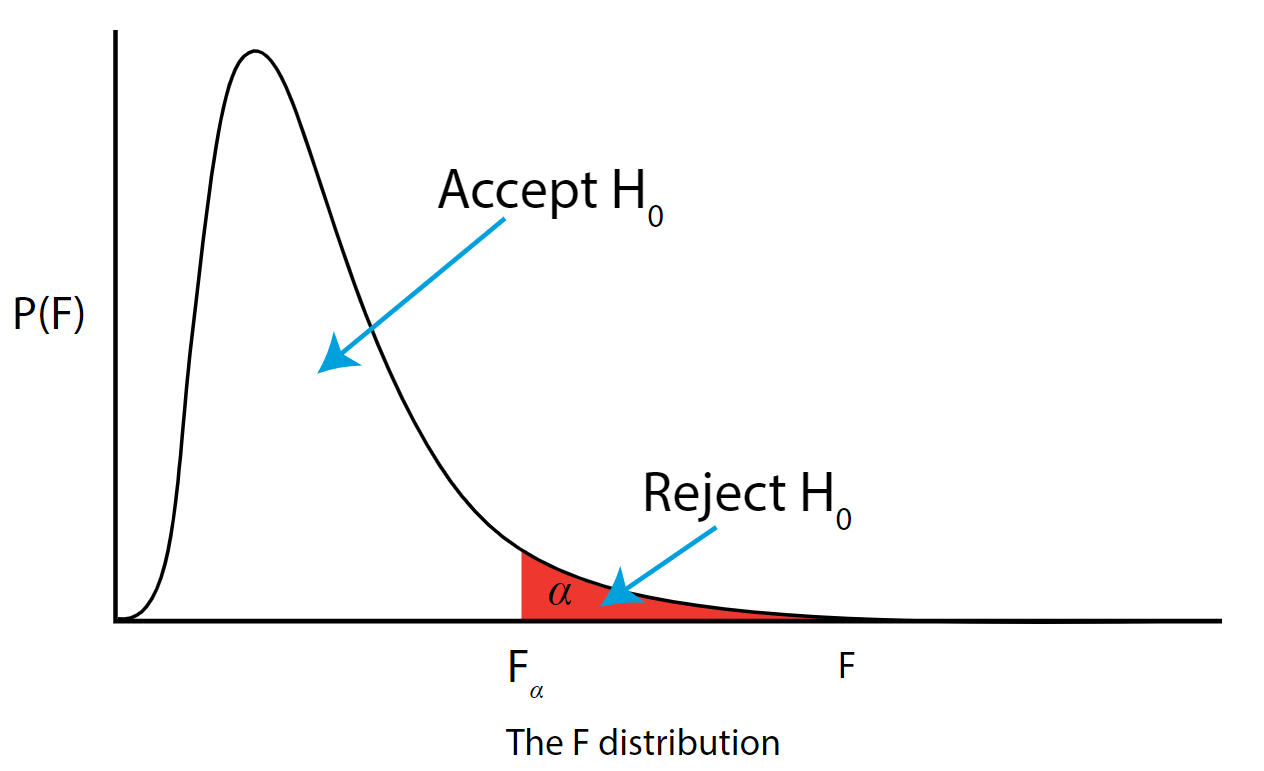
Step 6: Construct Acceptance / Rejection regions

As with all other test statistics, a threshold (critical) value of \(F\) is established. This \(F\) value can be obtained from statistical tables or software and is referred to as \(F_{\text{critical}}\) or \(F_{\alpha}\). As a reminder, this critical value is the minimum value for the test statistic (in this case the F test) for us to be able to reject the null.

The \(F\) distribution, \(F_{\alpha}\), and the location of acceptance and rejection regions are shown in the graph below:

Step 7: Based on steps 5 and 6, draw a conclusion about H0

If the \(F_{\text{\calculated}}\) from the data is larger than the \(F_{\alpha}\), then you are in the rejection region and you can reject the null hypothesis with \((1 - \alpha)\) level of confidence.

Note that modern statistical software condenses steps 6 and 7 by providing a \(p\)-value. The \(p\)-value here is the probability of getting an \(F_{\text{calculated}}\) even greater than what you observe assuming the null hypothesis is true. If by chance, the \(F_{\text{calculated}} = F_{\alpha}\), then the \(p\)-value would exactly equal \(\alpha\). With larger \(F_{\text{calculated}}\) values, we move further into the rejection region and the \(p\) - value becomes less than \(\alpha\). So the decision rule is as follows:

If the \(p\) - value obtained from the ANOVA is less than \(\alpha\), then reject \(H_{0}\) and accept \(H_{A}\).

If you are not familiar with this material, we suggest that you review course materials from your basic statistics course.

Hypothesis Testing for Means & Proportions

Lisa Sullivan, PhD

Professor of Biostatistics

Boston University School of Public Health

Introduction

This is the first of three modules that will addresses the second area of statistical inference, which is hypothesis testing, in which a specific statement or hypothesis is generated about a population parameter, and sample statistics are used to assess the likelihood that the hypothesis is true. The hypothesis is based on available information and the investigator's belief about the population parameters. The process of hypothesis testing involves setting up two competing hypotheses, the null hypothesis and the alternate hypothesis. One selects a random sample (or multiple samples when there are more comparison groups), computes summary statistics and then assesses the likelihood that the sample data support the research or alternative hypothesis. Similar to estimation, the process of hypothesis testing is based on probability theory and the Central Limit Theorem.  

This module will focus on hypothesis testing for means and proportions. The next two modules in this series will address analysis of variance and chi-squared tests. 

Learning Objectives

After completing this module, the student will be able to:

• Define null and research hypothesis, test statistic, level of significance and decision rule
• Distinguish between Type I and Type II errors and discuss the implications of each
• Explain the difference between one and two sided tests of hypothesis
• Estimate and interpret p-values
• Explain the relationship between confidence interval estimates and p-values in drawing inferences
• Differentiate hypothesis testing procedures based on type of outcome variable and number of sample

Introduction to Hypothesis Testing

Techniques for hypothesis testing  .

The techniques for hypothesis testing depend on

• the type of outcome variable being analyzed (continuous, dichotomous, discrete)
• the number of comparison groups in the investigation
• whether the comparison groups are independent (i.e., physically separate such as men versus women) or dependent (i.e., matched or paired such as pre- and post-assessments on the same participants).

In estimation we focused explicitly on techniques for one and two samples and discussed estimation for a specific parameter (e.g., the mean or proportion of a population), for differences (e.g., difference in means, the risk difference) and ratios (e.g., the relative risk and odds ratio). Here we will focus on procedures for one and two samples when the outcome is either continuous (and we focus on means) or dichotomous (and we focus on proportions).

General Approach: A Simple Example

The Centers for Disease Control (CDC) reported on trends in weight, height and body mass index from the 1960's through 2002. 1 The general trend was that Americans were much heavier and slightly taller in 2002 as compared to 1960; both men and women gained approximately 24 pounds, on average, between 1960 and 2002.   In 2002, the mean weight for men was reported at 191 pounds. Suppose that an investigator hypothesizes that weights are even higher in 2006 (i.e., that the trend continued over the subsequent 4 years). The research hypothesis is that the mean weight in men in 2006 is more than 191 pounds. The null hypothesis is that there is no change in weight, and therefore the mean weight is still 191 pounds in 2006.  

In order to test the hypotheses, we select a random sample of American males in 2006 and measure their weights. Suppose we have resources available to recruit n=100 men into our sample. We weigh each participant and compute summary statistics on the sample data. Suppose in the sample we determine the following:

Do the sample data support the null or research hypothesis? The sample mean of 197.1 is numerically higher than 191. However, is this difference more than would be expected by chance? In hypothesis testing, we assume that the null hypothesis holds until proven otherwise. We therefore need to determine the likelihood of observing a sample mean of 197.1 or higher when the true population mean is 191 (i.e., if the null hypothesis is true or under the null hypothesis). We can compute this probability using the Central Limit Theorem. Specifically,

(Notice that we use the sample standard deviation in computing the Z score. This is generally an appropriate substitution as long as the sample size is large, n > 30. Thus, there is less than a 1% probability of observing a sample mean as large as 197.1 when the true population mean is 191. Do you think that the null hypothesis is likely true? Based on how unlikely it is to observe a sample mean of 197.1 under the null hypothesis (i.e., <1% probability), we might infer, from our data, that the null hypothesis is probably not true.

Suppose that the sample data had turned out differently. Suppose that we instead observed the following in 2006:

How likely it is to observe a sample mean of 192.1 or higher when the true population mean is 191 (i.e., if the null hypothesis is true)? We can again compute this probability using the Central Limit Theorem. Specifically,

There is a 33.4% probability of observing a sample mean as large as 192.1 when the true population mean is 191. Do you think that the null hypothesis is likely true?  

Neither of the sample means that we obtained allows us to know with certainty whether the null hypothesis is true or not. However, our computations suggest that, if the null hypothesis were true, the probability of observing a sample mean >197.1 is less than 1%. In contrast, if the null hypothesis were true, the probability of observing a sample mean >192.1 is about 33%. We can't know whether the null hypothesis is true, but the sample that provided a mean value of 197.1 provides much stronger evidence in favor of rejecting the null hypothesis, than the sample that provided a mean value of 192.1. Note that this does not mean that a sample mean of 192.1 indicates that the null hypothesis is true; it just doesn't provide compelling evidence to reject it.

In essence, hypothesis testing is a procedure to compute a probability that reflects the strength of the evidence (based on a given sample) for rejecting the null hypothesis. In hypothesis testing, we determine a threshold or cut-off point (called the critical value) to decide when to believe the null hypothesis and when to believe the research hypothesis. It is important to note that it is possible to observe any sample mean when the true population mean is true (in this example equal to 191), but some sample means are very unlikely. Based on the two samples above it would seem reasonable to believe the research hypothesis when x̄ = 197.1, but to believe the null hypothesis when x̄ =192.1. What we need is a threshold value such that if x̄ is above that threshold then we believe that H 1 is true and if x̄ is below that threshold then we believe that H 0 is true. The difficulty in determining a threshold for x̄ is that it depends on the scale of measurement. In this example, the threshold, sometimes called the critical value, might be 195 (i.e., if the sample mean is 195 or more then we believe that H 1 is true and if the sample mean is less than 195 then we believe that H 0 is true). Suppose we are interested in assessing an increase in blood pressure over time, the critical value will be different because blood pressures are measured in millimeters of mercury (mmHg) as opposed to in pounds. In the following we will explain how the critical value is determined and how we handle the issue of scale.

First, to address the issue of scale in determining the critical value, we convert our sample data (in particular the sample mean) into a Z score. We know from the module on probability that the center of the Z distribution is zero and extreme values are those that exceed 2 or fall below -2. Z scores above 2 and below -2 represent approximately 5% of all Z values. If the observed sample mean is close to the mean specified in H 0 (here m =191), then Z will be close to zero. If the observed sample mean is much larger than the mean specified in H 0 , then Z will be large.  

In hypothesis testing, we select a critical value from the Z distribution. This is done by first determining what is called the level of significance, denoted α ("alpha"). What we are doing here is drawing a line at extreme values. The level of significance is the probability that we reject the null hypothesis (in favor of the alternative) when it is actually true and is also called the Type I error rate.

α = Level of significance = P(Type I error) = P(Reject H 0 | H 0 is true).

Because α is a probability, it ranges between 0 and 1. The most commonly used value in the medical literature for α is 0.05, or 5%. Thus, if an investigator selects α=0.05, then they are allowing a 5% probability of incorrectly rejecting the null hypothesis in favor of the alternative when the null is in fact true. Depending on the circumstances, one might choose to use a level of significance of 1% or 10%. For example, if an investigator wanted to reject the null only if there were even stronger evidence than that ensured with α=0.05, they could choose a =0.01as their level of significance. The typical values for α are 0.01, 0.05 and 0.10, with α=0.05 the most commonly used value.  

Suppose in our weight study we select α=0.05. We need to determine the value of Z that holds 5% of the values above it (see below).

The critical value of Z for α =0.05 is Z = 1.645 (i.e., 5% of the distribution is above Z=1.645). With this value we can set up what is called our decision rule for the test. The rule is to reject H 0 if the Z score is 1.645 or more.  

With the first sample we have

Because 2.38 > 1.645, we reject the null hypothesis. (The same conclusion can be drawn by comparing the 0.0087 probability of observing a sample mean as extreme as 197.1 to the level of significance of 0.05. If the observed probability is smaller than the level of significance we reject H 0 ). Because the Z score exceeds the critical value, we conclude that the mean weight for men in 2006 is more than 191 pounds, the value reported in 2002. If we observed the second sample (i.e., sample mean =192.1), we would not be able to reject the null hypothesis because the Z score is 0.43 which is not in the rejection region (i.e., the region in the tail end of the curve above 1.645). With the second sample we do not have sufficient evidence (because we set our level of significance at 5%) to conclude that weights have increased. Again, the same conclusion can be reached by comparing probabilities. The probability of observing a sample mean as extreme as 192.1 is 33.4% which is not below our 5% level of significance.

Hypothesis Testing: Upper-, Lower, and Two Tailed Tests

The procedure for hypothesis testing is based on the ideas described above. Specifically, we set up competing hypotheses, select a random sample from the population of interest and compute summary statistics. We then determine whether the sample data supports the null or alternative hypotheses. The procedure can be broken down into the following five steps.  

• Step 1. Set up hypotheses and select the level of significance α.

H 0 : Null hypothesis (no change, no difference);  

H 1 : Research hypothesis (investigator's belief); α =0.05

• Step 2. Select the appropriate test statistic.  

The test statistic is a single number that summarizes the sample information.   An example of a test statistic is the Z statistic computed as follows:

When the sample size is small, we will use t statistics (just as we did when constructing confidence intervals for small samples). As we present each scenario, alternative test statistics are provided along with conditions for their appropriate use.

• Step 3.  Set up decision rule.  

The decision rule is a statement that tells under what circumstances to reject the null hypothesis. The decision rule is based on specific values of the test statistic (e.g., reject H 0 if Z > 1.645). The decision rule for a specific test depends on 3 factors: the research or alternative hypothesis, the test statistic and the level of significance. Each is discussed below.

• The decision rule depends on whether an upper-tailed, lower-tailed, or two-tailed test is proposed. In an upper-tailed test the decision rule has investigators reject H 0 if the test statistic is larger than the critical value. In a lower-tailed test the decision rule has investigators reject H 0 if the test statistic is smaller than the critical value.  In a two-tailed test the decision rule has investigators reject H 0 if the test statistic is extreme, either larger than an upper critical value or smaller than a lower critical value.
• The exact form of the test statistic is also important in determining the decision rule. If the test statistic follows the standard normal distribution (Z), then the decision rule will be based on the standard normal distribution. If the test statistic follows the t distribution, then the decision rule will be based on the t distribution. The appropriate critical value will be selected from the t distribution again depending on the specific alternative hypothesis and the level of significance.  
• The third factor is the level of significance. The level of significance which is selected in Step 1 (e.g., α =0.05) dictates the critical value.   For example, in an upper tailed Z test, if α =0.05 then the critical value is Z=1.645.  

The following figures illustrate the rejection regions defined by the decision rule for upper-, lower- and two-tailed Z tests with α=0.05. Notice that the rejection regions are in the upper, lower and both tails of the curves, respectively. The decision rules are written below each figure.

Rejection Region for Lower-Tailed Z Test (H 1 : μ < μ 0 ) with α =0.05

The decision rule is: Reject H 0 if Z < 1.645.

Rejection Region for Two-Tailed Z Test (H 1 : μ ≠ μ 0 ) with α =0.05

The decision rule is: Reject H 0 if Z < -1.960 or if Z > 1.960.

The complete table of critical values of Z for upper, lower and two-tailed tests can be found in the table of Z values to the right in "Other Resources."

Critical values of t for upper, lower and two-tailed tests can be found in the table of t values in "Other Resources."

• Step 4. Compute the test statistic.  

Here we compute the test statistic by substituting the observed sample data into the test statistic identified in Step 2.

• Step 5. Conclusion.  

The final conclusion is made by comparing the test statistic (which is a summary of the information observed in the sample) to the decision rule. The final conclusion will be either to reject the null hypothesis (because the sample data are very unlikely if the null hypothesis is true) or not to reject the null hypothesis (because the sample data are not very unlikely).  

If the null hypothesis is rejected, then an exact significance level is computed to describe the likelihood of observing the sample data assuming that the null hypothesis is true. The exact level of significance is called the p-value and it will be less than the chosen level of significance if we reject H 0 .

Statistical computing packages provide exact p-values as part of their standard output for hypothesis tests. In fact, when using a statistical computing package, the steps outlined about can be abbreviated. The hypotheses (step 1) should always be set up in advance of any analysis and the significance criterion should also be determined (e.g., α =0.05). Statistical computing packages will produce the test statistic (usually reporting the test statistic as t) and a p-value. The investigator can then determine statistical significance using the following: If p < α then reject H 0 .  

• Step 1. Set up hypotheses and determine level of significance

H 0 : μ = 191 H 1 : μ > 191                 α =0.05

The research hypothesis is that weights have increased, and therefore an upper tailed test is used.

• Step 2. Select the appropriate test statistic.

Because the sample size is large (n > 30) the appropriate test statistic is

• Step 3. Set up decision rule.  

In this example, we are performing an upper tailed test (H 1 : μ> 191), with a Z test statistic and selected α =0.05.   Reject H 0 if Z > 1.645.

We now substitute the sample data into the formula for the test statistic identified in Step 2.  

We reject H 0 because 2.38 > 1.645. We have statistically significant evidence at a =0.05, to show that the mean weight in men in 2006 is more than 191 pounds. Because we rejected the null hypothesis, we now approximate the p-value which is the likelihood of observing the sample data if the null hypothesis is true. An alternative definition of the p-value is the smallest level of significance where we can still reject H 0 . In this example, we observed Z=2.38 and for α=0.05, the critical value was 1.645. Because 2.38 exceeded 1.645 we rejected H 0 . In our conclusion we reported a statistically significant increase in mean weight at a 5% level of significance. Using the table of critical values for upper tailed tests, we can approximate the p-value. If we select α=0.025, the critical value is 1.96, and we still reject H 0 because 2.38 > 1.960. If we select α=0.010 the critical value is 2.326, and we still reject H 0 because 2.38 > 2.326. However, if we select α=0.005, the critical value is 2.576, and we cannot reject H 0 because 2.38 < 2.576. Therefore, the smallest α where we still reject H 0 is 0.010. This is the p-value. A statistical computing package would produce a more precise p-value which would be in between 0.005 and 0.010. Here we are approximating the p-value and would report p < 0.010.                  

Type I and Type II Errors

In all tests of hypothesis, there are two types of errors that can be committed. The first is called a Type I error and refers to the situation where we incorrectly reject H 0 when in fact it is true. This is also called a false positive result (as we incorrectly conclude that the research hypothesis is true when in fact it is not). When we run a test of hypothesis and decide to reject H 0 (e.g., because the test statistic exceeds the critical value in an upper tailed test) then either we make a correct decision because the research hypothesis is true or we commit a Type I error. The different conclusions are summarized in the table below. Note that we will never know whether the null hypothesis is really true or false (i.e., we will never know which row of the following table reflects reality).

Table - Conclusions in Test of Hypothesis

In the first step of the hypothesis test, we select a level of significance, α, and α= P(Type I error). Because we purposely select a small value for α, we control the probability of committing a Type I error. For example, if we select α=0.05, and our test tells us to reject H 0 , then there is a 5% probability that we commit a Type I error. Most investigators are very comfortable with this and are confident when rejecting H 0 that the research hypothesis is true (as it is the more likely scenario when we reject H 0 ).

When we run a test of hypothesis and decide not to reject H 0 (e.g., because the test statistic is below the critical value in an upper tailed test) then either we make a correct decision because the null hypothesis is true or we commit a Type II error. Beta (β) represents the probability of a Type II error and is defined as follows: β=P(Type II error) = P(Do not Reject H 0 | H 0 is false). Unfortunately, we cannot choose β to be small (e.g., 0.05) to control the probability of committing a Type II error because β depends on several factors including the sample size, α, and the research hypothesis. When we do not reject H 0 , it may be very likely that we are committing a Type II error (i.e., failing to reject H 0 when in fact it is false). Therefore, when tests are run and the null hypothesis is not rejected we often make a weak concluding statement allowing for the possibility that we might be committing a Type II error. If we do not reject H 0 , we conclude that we do not have significant evidence to show that H 1 is true. We do not conclude that H 0 is true.

 The most common reason for a Type II error is a small sample size.

Tests with One Sample, Continuous Outcome

Hypothesis testing applications with a continuous outcome variable in a single population are performed according to the five-step procedure outlined above. A key component is setting up the null and research hypotheses. The objective is to compare the mean in a single population to known mean (μ 0 ). The known value is generally derived from another study or report, for example a study in a similar, but not identical, population or a study performed some years ago. The latter is called a historical control. It is important in setting up the hypotheses in a one sample test that the mean specified in the null hypothesis is a fair and reasonable comparator. This will be discussed in the examples that follow.

Test Statistics for Testing H 0 : μ= μ 0

• if n > 30
• if n < 30

Note that statistical computing packages will use the t statistic exclusively and make the necessary adjustments for comparing the test statistic to appropriate values from probability tables to produce a p-value. 

The National Center for Health Statistics (NCHS) published a report in 2005 entitled Health, United States, containing extensive information on major trends in the health of Americans. Data are provided for the US population as a whole and for specific ages, sexes and races.  The NCHS report indicated that in 2002 Americans paid an average of $3,302 per year on health care and prescription drugs. An investigator hypothesizes that in 2005 expenditures have decreased primarily due to the availability of generic drugs. To test the hypothesis, a sample of 100 Americans are selected and their expenditures on health care and prescription drugs in 2005 are measured.   The sample data are summarized as follows: n=100, x̄

=$3,190 and s=$890. Is there statistical evidence of a reduction in expenditures on health care and prescription drugs in 2005? Is the sample mean of $3,190 evidence of a true reduction in the mean or is it within chance fluctuation? We will run the test using the five-step approach. 

• Step 1.  Set up hypotheses and determine level of significance

H 0 : μ = 3,302 H 1 : μ < 3,302           α =0.05

The research hypothesis is that expenditures have decreased, and therefore a lower-tailed test is used.

This is a lower tailed test, using a Z statistic and a 5% level of significance.   Reject H 0 if Z < -1.645.

•   Step 4. Compute the test statistic.  

We do not reject H 0 because -1.26 > -1.645. We do not have statistically significant evidence at α=0.05 to show that the mean expenditures on health care and prescription drugs are lower in 2005 than the mean of $3,302 reported in 2002.  

Recall that when we fail to reject H 0 in a test of hypothesis that either the null hypothesis is true (here the mean expenditures in 2005 are the same as those in 2002 and equal to $3,302) or we committed a Type II error (i.e., we failed to reject H 0 when in fact it is false). In summarizing this test, we conclude that we do not have sufficient evidence to reject H 0 . We do not conclude that H 0 is true, because there may be a moderate to high probability that we committed a Type II error. It is possible that the sample size is not large enough to detect a difference in mean expenditures.      

The NCHS reported that the mean total cholesterol level in 2002 for all adults was 203. Total cholesterol levels in participants who attended the seventh examination of the Offspring in the Framingham Heart Study are summarized as follows: n=3,310, x̄ =200.3, and s=36.8. Is there statistical evidence of a difference in mean cholesterol levels in the Framingham Offspring?

Here we want to assess whether the sample mean of 200.3 in the Framingham sample is statistically significantly different from 203 (i.e., beyond what we would expect by chance). We will run the test using the five-step approach.

H 0 : μ= 203 H 1 : μ≠ 203                       α=0.05

The research hypothesis is that cholesterol levels are different in the Framingham Offspring, and therefore a two-tailed test is used.

•   Step 3. Set up decision rule.  

This is a two-tailed test, using a Z statistic and a 5% level of significance. Reject H 0 if Z < -1.960 or is Z > 1.960.

We reject H 0 because -4.22 ≤ -1. .960. We have statistically significant evidence at α=0.05 to show that the mean total cholesterol level in the Framingham Offspring is different from the national average of 203 reported in 2002.   Because we reject H 0 , we also approximate a p-value. Using the two-sided significance levels, p < 0.0001.  

Statistical Significance versus Clinical (Practical) Significance

This example raises an important concept of statistical versus clinical or practical significance. From a statistical standpoint, the total cholesterol levels in the Framingham sample are highly statistically significantly different from the national average with p < 0.0001 (i.e., there is less than a 0.01% chance that we are incorrectly rejecting the null hypothesis). However, the sample mean in the Framingham Offspring study is 200.3, less than 3 units different from the national mean of 203. The reason that the data are so highly statistically significant is due to the very large sample size. It is always important to assess both statistical and clinical significance of data. This is particularly relevant when the sample size is large. Is a 3 unit difference in total cholesterol a meaningful difference?  

Consider again the NCHS-reported mean total cholesterol level in 2002 for all adults of 203. Suppose a new drug is proposed to lower total cholesterol. A study is designed to evaluate the efficacy of the drug in lowering cholesterol.   Fifteen patients are enrolled in the study and asked to take the new drug for 6 weeks. At the end of 6 weeks, each patient's total cholesterol level is measured and the sample statistics are as follows:   n=15, x̄ =195.9 and s=28.7. Is there statistical evidence of a reduction in mean total cholesterol in patients after using the new drug for 6 weeks? We will run the test using the five-step approach. 

H 0 : μ= 203 H 1 : μ< 203                   α=0.05

•  Step 2. Select the appropriate test statistic.  

Because the sample size is small (n<30) the appropriate test statistic is

This is a lower tailed test, using a t statistic and a 5% level of significance. In order to determine the critical value of t, we need degrees of freedom, df, defined as df=n-1. In this example df=15-1=14. The critical value for a lower tailed test with df=14 and a =0.05 is -2.145 and the decision rule is as follows:   Reject H 0 if t < -2.145.

We do not reject H 0 because -0.96 > -2.145. We do not have statistically significant evidence at α=0.05 to show that the mean total cholesterol level is lower than the national mean in patients taking the new drug for 6 weeks. Again, because we failed to reject the null hypothesis we make a weaker concluding statement allowing for the possibility that we may have committed a Type II error (i.e., failed to reject H 0 when in fact the drug is efficacious).

This example raises an important issue in terms of study design. In this example we assume in the null hypothesis that the mean cholesterol level is 203. This is taken to be the mean cholesterol level in patients without treatment. Is this an appropriate comparator? Alternative and potentially more efficient study designs to evaluate the effect of the new drug could involve two treatment groups, where one group receives the new drug and the other does not, or we could measure each patient's baseline or pre-treatment cholesterol level and then assess changes from baseline to 6 weeks post-treatment. These designs are also discussed here.

Video - Comparing a Sample Mean to Known Population Mean (8:20)

Link to transcript of the video

Tests with One Sample, Dichotomous Outcome

Hypothesis testing applications with a dichotomous outcome variable in a single population are also performed according to the five-step procedure. Similar to tests for means, a key component is setting up the null and research hypotheses. The objective is to compare the proportion of successes in a single population to a known proportion (p 0 ). That known proportion is generally derived from another study or report and is sometimes called a historical control. It is important in setting up the hypotheses in a one sample test that the proportion specified in the null hypothesis is a fair and reasonable comparator.    

In one sample tests for a dichotomous outcome, we set up our hypotheses against an appropriate comparator. We select a sample and compute descriptive statistics on the sample data. Specifically, we compute the sample size (n) and the sample proportion which is computed by taking the ratio of the number of successes to the sample size,

We then determine the appropriate test statistic (Step 2) for the hypothesis test. The formula for the test statistic is given below.

Test Statistic for Testing H 0 : p = p 0

if min(np 0 , n(1-p 0 )) > 5

The formula above is appropriate for large samples, defined when the smaller of np 0 and n(1-p 0 ) is at least 5. This is similar, but not identical, to the condition required for appropriate use of the confidence interval formula for a population proportion, i.e.,

Here we use the proportion specified in the null hypothesis as the true proportion of successes rather than the sample proportion. If we fail to satisfy the condition, then alternative procedures, called exact methods must be used to test the hypothesis about the population proportion.

Example:  

The NCHS report indicated that in 2002 the prevalence of cigarette smoking among American adults was 21.1%.  Data on prevalent smoking in n=3,536 participants who attended the seventh examination of the Offspring in the Framingham Heart Study indicated that 482/3,536 = 13.6% of the respondents were currently smoking at the time of the exam. Suppose we want to assess whether the prevalence of smoking is lower in the Framingham Offspring sample given the focus on cardiovascular health in that community. Is there evidence of a statistically lower prevalence of smoking in the Framingham Offspring study as compared to the prevalence among all Americans?

H 0 : p = 0.211 H 1 : p < 0.211                     α=0.05

We must first check that the sample size is adequate.   Specifically, we need to check min(np 0 , n(1-p 0 )) = min( 3,536(0.211), 3,536(1-0.211))=min(746, 2790)=746. The sample size is more than adequate so the following formula can be used:

This is a lower tailed test, using a Z statistic and a 5% level of significance. Reject H 0 if Z < -1.645.

We reject H 0 because -10.93 < -1.645. We have statistically significant evidence at α=0.05 to show that the prevalence of smoking in the Framingham Offspring is lower than the prevalence nationally (21.1%). Here, p < 0.0001.  

The NCHS report indicated that in 2002, 75% of children aged 2 to 17 saw a dentist in the past year. An investigator wants to assess whether use of dental services is similar in children living in the city of Boston. A sample of 125 children aged 2 to 17 living in Boston are surveyed and 64 reported seeing a dentist over the past 12 months. Is there a significant difference in use of dental services between children living in Boston and the national data?

Calculate this on your own before checking the answer.

Video - Hypothesis Test for One Sample and a Dichotomous Outcome (3:55)

Tests with Two Independent Samples, Continuous Outcome

There are many applications where it is of interest to compare two independent groups with respect to their mean scores on a continuous outcome. Here we compare means between groups, but rather than generating an estimate of the difference, we will test whether the observed difference (increase, decrease or difference) is statistically significant or not. Remember, that hypothesis testing gives an assessment of statistical significance, whereas estimation gives an estimate of effect and both are important.

Here we discuss the comparison of means when the two comparison groups are independent or physically separate. The two groups might be determined by a particular attribute (e.g., sex, diagnosis of cardiovascular disease) or might be set up by the investigator (e.g., participants assigned to receive an experimental treatment or placebo). The first step in the analysis involves computing descriptive statistics on each of the two samples. Specifically, we compute the sample size, mean and standard deviation in each sample and we denote these summary statistics as follows:

for sample 1:

for sample 2:

The designation of sample 1 and sample 2 is arbitrary. In a clinical trial setting the convention is to call the treatment group 1 and the control group 2. However, when comparing men and women, for example, either group can be 1 or 2.  

In the two independent samples application with a continuous outcome, the parameter of interest in the test of hypothesis is the difference in population means, μ 1 -μ 2 . The null hypothesis is always that there is no difference between groups with respect to means, i.e.,

The null hypothesis can also be written as follows: H 0 : μ 1 = μ 2 . In the research hypothesis, an investigator can hypothesize that the first mean is larger than the second (H 1 : μ 1 > μ 2 ), that the first mean is smaller than the second (H 1 : μ 1 < μ 2 ), or that the means are different (H 1 : μ 1 ≠ μ 2 ). The three different alternatives represent upper-, lower-, and two-tailed tests, respectively. The following test statistics are used to test these hypotheses.

Test Statistics for Testing H 0 : μ 1 = μ 2

• if n 1 > 30 and n 2 > 30
• if n 1 < 30 or n 2 < 30

NOTE: The formulas above assume equal variability in the two populations (i.e., the population variances are equal, or s 1 2 = s 2 2 ). This means that the outcome is equally variable in each of the comparison populations. For analysis, we have samples from each of the comparison populations. If the sample variances are similar, then the assumption about variability in the populations is probably reasonable. As a guideline, if the ratio of the sample variances, s 1 2 /s 2 2 is between 0.5 and 2 (i.e., if one variance is no more than double the other), then the formulas above are appropriate. If the ratio of the sample variances is greater than 2 or less than 0.5 then alternative formulas must be used to account for the heterogeneity in variances.    

The test statistics include Sp, which is the pooled estimate of the common standard deviation (again assuming that the variances in the populations are similar) computed as the weighted average of the standard deviations in the samples as follows:

Because we are assuming equal variances between groups, we pool the information on variability (sample variances) to generate an estimate of the variability in the population. Note: Because Sp is a weighted average of the standard deviations in the sample, Sp will always be in between s 1 and s 2 .)

Data measured on n=3,539 participants who attended the seventh examination of the Offspring in the Framingham Heart Study are shown below.  

Suppose we now wish to assess whether there is a statistically significant difference in mean systolic blood pressures between men and women using a 5% level of significance.  

H 0 : μ 1 = μ 2

H 1 : μ 1 ≠ μ 2                       α=0.05

Because both samples are large ( > 30), we can use the Z test statistic as opposed to t. Note that statistical computing packages use t throughout. Before implementing the formula, we first check whether the assumption of equality of population variances is reasonable. The guideline suggests investigating the ratio of the sample variances, s 1 2 /s 2 2 . Suppose we call the men group 1 and the women group 2. Again, this is arbitrary; it only needs to be noted when interpreting the results. The ratio of the sample variances is 17.5 2 /20.1 2 = 0.76, which falls between 0.5 and 2 suggesting that the assumption of equality of population variances is reasonable. The appropriate test statistic is

We now substitute the sample data into the formula for the test statistic identified in Step 2. Before substituting, we will first compute Sp, the pooled estimate of the common standard deviation.

Notice that the pooled estimate of the common standard deviation, Sp, falls in between the standard deviations in the comparison groups (i.e., 17.5 and 20.1). Sp is slightly closer in value to the standard deviation in the women (20.1) as there were slightly more women in the sample.   Recall, Sp is a weight average of the standard deviations in the comparison groups, weighted by the respective sample sizes.  

Now the test statistic:

We reject H 0 because 2.66 > 1.960. We have statistically significant evidence at α=0.05 to show that there is a difference in mean systolic blood pressures between men and women. The p-value is p < 0.010.  

Here again we find that there is a statistically significant difference in mean systolic blood pressures between men and women at p < 0.010. Notice that there is a very small difference in the sample means (128.2-126.5 = 1.7 units), but this difference is beyond what would be expected by chance. Is this a clinically meaningful difference? The large sample size in this example is driving the statistical significance. A 95% confidence interval for the difference in mean systolic blood pressures is: 1.7 + 1.26 or (0.44, 2.96). The confidence interval provides an assessment of the magnitude of the difference between means whereas the test of hypothesis and p-value provide an assessment of the statistical significance of the difference.  

Above we performed a study to evaluate a new drug designed to lower total cholesterol. The study involved one sample of patients, each patient took the new drug for 6 weeks and had their cholesterol measured. As a means of evaluating the efficacy of the new drug, the mean total cholesterol following 6 weeks of treatment was compared to the NCHS-reported mean total cholesterol level in 2002 for all adults of 203. At the end of the example, we discussed the appropriateness of the fixed comparator as well as an alternative study design to evaluate the effect of the new drug involving two treatment groups, where one group receives the new drug and the other does not. Here, we revisit the example with a concurrent or parallel control group, which is very typical in randomized controlled trials or clinical trials (refer to the EP713 module on Clinical Trials).  

A new drug is proposed to lower total cholesterol. A randomized controlled trial is designed to evaluate the efficacy of the medication in lowering cholesterol. Thirty participants are enrolled in the trial and are randomly assigned to receive either the new drug or a placebo. The participants do not know which treatment they are assigned. Each participant is asked to take the assigned treatment for 6 weeks. At the end of 6 weeks, each patient's total cholesterol level is measured and the sample statistics are as follows.

Is there statistical evidence of a reduction in mean total cholesterol in patients taking the new drug for 6 weeks as compared to participants taking placebo? We will run the test using the five-step approach.

H 0 : μ 1 = μ 2 H 1 : μ 1 < μ 2                         α=0.05

Because both samples are small (< 30), we use the t test statistic. Before implementing the formula, we first check whether the assumption of equality of population variances is reasonable. The ratio of the sample variances, s 1 2 /s 2 2 =28.7 2 /30.3 2 = 0.90, which falls between 0.5 and 2, suggesting that the assumption of equality of population variances is reasonable. The appropriate test statistic is:

This is a lower-tailed test, using a t statistic and a 5% level of significance. The appropriate critical value can be found in the t Table (in More Resources to the right). In order to determine the critical value of t we need degrees of freedom, df, defined as df=n 1 +n 2 -2 = 15+15-2=28. The critical value for a lower tailed test with df=28 and α=0.05 is -1.701 and the decision rule is: Reject H 0 if t < -1.701.

Now the test statistic,

We reject H 0 because -2.92 < -1.701. We have statistically significant evidence at α=0.05 to show that the mean total cholesterol level is lower in patients taking the new drug for 6 weeks as compared to patients taking placebo, p < 0.005.

The clinical trial in this example finds a statistically significant reduction in total cholesterol, whereas in the previous example where we had a historical control (as opposed to a parallel control group) we did not demonstrate efficacy of the new drug. Notice that the mean total cholesterol level in patients taking placebo is 217.4 which is very different from the mean cholesterol reported among all Americans in 2002 of 203 and used as the comparator in the prior example. The historical control value may not have been the most appropriate comparator as cholesterol levels have been increasing over time. In the next section, we present another design that can be used to assess the efficacy of the new drug.

Video - Comparison of Two Independent Samples With a Continuous Outcome (8:02)

Tests with Matched Samples, Continuous Outcome

In the previous section we compared two groups with respect to their mean scores on a continuous outcome. An alternative study design is to compare matched or paired samples. The two comparison groups are said to be dependent, and the data can arise from a single sample of participants where each participant is measured twice (possibly before and after an intervention) or from two samples that are matched on specific characteristics (e.g., siblings). When the samples are dependent, we focus on difference scores in each participant or between members of a pair and the test of hypothesis is based on the mean difference, μ d . The null hypothesis again reflects "no difference" and is stated as H 0 : μ d =0 . Note that there are some instances where it is of interest to test whether there is a difference of a particular magnitude (e.g., μ d =5) but in most instances the null hypothesis reflects no difference (i.e., μ d =0).  

The appropriate formula for the test of hypothesis depends on the sample size. The formulas are shown below and are identical to those we presented for estimating the mean of a single sample presented (e.g., when comparing against an external or historical control), except here we focus on difference scores.

Test Statistics for Testing H 0 : μ d =0

A new drug is proposed to lower total cholesterol and a study is designed to evaluate the efficacy of the drug in lowering cholesterol. Fifteen patients agree to participate in the study and each is asked to take the new drug for 6 weeks. However, before starting the treatment, each patient's total cholesterol level is measured. The initial measurement is a pre-treatment or baseline value. After taking the drug for 6 weeks, each patient's total cholesterol level is measured again and the data are shown below. The rightmost column contains difference scores for each patient, computed by subtracting the 6 week cholesterol level from the baseline level. The differences represent the reduction in total cholesterol over 4 weeks. (The differences could have been computed by subtracting the baseline total cholesterol level from the level measured at 6 weeks. The way in which the differences are computed does not affect the outcome of the analysis only the interpretation.)

Because the differences are computed by subtracting the cholesterols measured at 6 weeks from the baseline values, positive differences indicate reductions and negative differences indicate increases (e.g., participant 12 increases by 2 units over 6 weeks). The goal here is to test whether there is a statistically significant reduction in cholesterol. Because of the way in which we computed the differences, we want to look for an increase in the mean difference (i.e., a positive reduction). In order to conduct the test, we need to summarize the differences. In this sample, we have

The calculations are shown below.  

Is there statistical evidence of a reduction in mean total cholesterol in patients after using the new medication for 6 weeks? We will run the test using the five-step approach.

H 0 : μ d = 0 H 1 : μ d > 0                 α=0.05

NOTE: If we had computed differences by subtracting the baseline level from the level measured at 6 weeks then negative differences would have reflected reductions and the research hypothesis would have been H 1 : μ d < 0. 

• Step 2 . Select the appropriate test statistic.

This is an upper-tailed test, using a t statistic and a 5% level of significance. The appropriate critical value can be found in the t Table at the right, with df=15-1=14. The critical value for an upper-tailed test with df=14 and α=0.05 is 2.145 and the decision rule is Reject H 0 if t > 2.145.

We now substitute the sample data into the formula for the test statistic identified in Step 2.

We reject H 0 because 4.61 > 2.145. We have statistically significant evidence at α=0.05 to show that there is a reduction in cholesterol levels over 6 weeks.  

Here we illustrate the use of a matched design to test the efficacy of a new drug to lower total cholesterol. We also considered a parallel design (randomized clinical trial) and a study using a historical comparator. It is extremely important to design studies that are best suited to detect a meaningful difference when one exists. There are often several alternatives and investigators work with biostatisticians to determine the best design for each application. It is worth noting that the matched design used here can be problematic in that observed differences may only reflect a "placebo" effect. All participants took the assigned medication, but is the observed reduction attributable to the medication or a result of these participation in a study.

Video - Hypothesis Testing With a Matched Sample and a Continuous Outcome (3:11)

Tests with Two Independent Samples, Dichotomous Outcome

There are several approaches that can be used to test hypotheses concerning two independent proportions. Here we present one approach - the chi-square test of independence is an alternative, equivalent, and perhaps more popular approach to the same analysis. Hypothesis testing with the chi-square test is addressed in the third module in this series: BS704_HypothesisTesting-ChiSquare.

In tests of hypothesis comparing proportions between two independent groups, one test is performed and results can be interpreted to apply to a risk difference, relative risk or odds ratio. As a reminder, the risk difference is computed by taking the difference in proportions between comparison groups, the risk ratio is computed by taking the ratio of proportions, and the odds ratio is computed by taking the ratio of the odds of success in the comparison groups. Because the null values for the risk difference, the risk ratio and the odds ratio are different, the hypotheses in tests of hypothesis look slightly different depending on which measure is used. When performing tests of hypothesis for the risk difference, relative risk or odds ratio, the convention is to label the exposed or treated group 1 and the unexposed or control group 2.      

For example, suppose a study is designed to assess whether there is a significant difference in proportions in two independent comparison groups. The test of interest is as follows:

H 0 : p 1 = p 2 versus H 1 : p 1 ≠ p 2 .  

The following are the hypothesis for testing for a difference in proportions using the risk difference, the risk ratio and the odds ratio. First, the hypotheses above are equivalent to the following:

• For the risk difference, H 0 : p 1 - p 2 = 0 versus H 1 : p 1 - p 2 ≠ 0 which are, by definition, equal to H 0 : RD = 0 versus H 1 : RD ≠ 0.
• If an investigator wants to focus on the risk ratio, the equivalent hypotheses are H 0 : RR = 1 versus H 1 : RR ≠ 1.
• If the investigator wants to focus on the odds ratio, the equivalent hypotheses are H 0 : OR = 1 versus H 1 : OR ≠ 1.  

Suppose a test is performed to test H 0 : RD = 0 versus H 1 : RD ≠ 0 and the test rejects H 0 at α=0.05. Based on this test we can conclude that there is significant evidence, α=0.05, of a difference in proportions, significant evidence that the risk difference is not zero, significant evidence that the risk ratio and odds ratio are not one. The risk difference is analogous to the difference in means when the outcome is continuous. Here the parameter of interest is the difference in proportions in the population, RD = p 1 -p 2 and the null value for the risk difference is zero. In a test of hypothesis for the risk difference, the null hypothesis is always H 0 : RD = 0. This is equivalent to H 0 : RR = 1 and H 0 : OR = 1. In the research hypothesis, an investigator can hypothesize that the first proportion is larger than the second (H 1 : p 1 > p 2 , which is equivalent to H 1 : RD > 0, H 1 : RR > 1 and H 1 : OR > 1), that the first proportion is smaller than the second (H 1 : p 1 < p 2 , which is equivalent to H 1 : RD < 0, H 1 : RR < 1 and H 1 : OR < 1), or that the proportions are different (H 1 : p 1 ≠ p 2 , which is equivalent to H 1 : RD ≠ 0, H 1 : RR ≠ 1 and H 1 : OR ≠

1). The three different alternatives represent upper-, lower- and two-tailed tests, respectively.  

The formula for the test of hypothesis for the difference in proportions is given below.

Test Statistics for Testing H 0 : p 1 = p

The formula above is appropriate for large samples, defined as at least 5 successes (np > 5) and at least 5 failures (n(1-p > 5)) in each of the two samples. If there are fewer than 5 successes or failures in either comparison group, then alternative procedures, called exact methods must be used to estimate the difference in population proportions.

The following table summarizes data from n=3,799 participants who attended the fifth examination of the Offspring in the Framingham Heart Study. The outcome of interest is prevalent CVD and we want to test whether the prevalence of CVD is significantly higher in smokers as compared to non-smokers.

The prevalence of CVD (or proportion of participants with prevalent CVD) among non-smokers is 298/3,055 = 0.0975 and the prevalence of CVD among current smokers is 81/744 = 0.1089. Here smoking status defines the comparison groups and we will call the current smokers group 1 (exposed) and the non-smokers (unexposed) group 2. The test of hypothesis is conducted below using the five step approach.

H 0 : p 1 = p 2     H 1 : p 1 ≠ p 2                 α=0.05

• Step 2.  Select the appropriate test statistic.  

We must first check that the sample size is adequate. Specifically, we need to ensure that we have at least 5 successes and 5 failures in each comparison group. In this example, we have more than enough successes (cases of prevalent CVD) and failures (persons free of CVD) in each comparison group. The sample size is more than adequate so the following formula can be used:

Reject H 0 if Z < -1.960 or if Z > 1.960.

We now substitute the sample data into the formula for the test statistic identified in Step 2. We first compute the overall proportion of successes:

We now substitute to compute the test statistic.

• Step 5. Conclusion.

We do not reject H 0 because -1.960 < 0.927 < 1.960. We do not have statistically significant evidence at α=0.05 to show that there is a difference in prevalent CVD between smokers and non-smokers.  

A 95% confidence interval for the difference in prevalent CVD (or risk difference) between smokers and non-smokers as 0.0114 + 0.0247, or between -0.0133 and 0.0361. Because the 95% confidence interval for the risk difference includes zero we again conclude that there is no statistically significant difference in prevalent CVD between smokers and non-smokers.    

Smoking has been shown over and over to be a risk factor for cardiovascular disease. What might explain the fact that we did not observe a statistically significant difference using data from the Framingham Heart Study? HINT: Here we consider prevalent CVD, would the results have been different if we considered incident CVD?

A randomized trial is designed to evaluate the effectiveness of a newly developed pain reliever designed to reduce pain in patients following joint replacement surgery. The trial compares the new pain reliever to the pain reliever currently in use (called the standard of care). A total of 100 patients undergoing joint replacement surgery agreed to participate in the trial. Patients were randomly assigned to receive either the new pain reliever or the standard pain reliever following surgery and were blind to the treatment assignment. Before receiving the assigned treatment, patients were asked to rate their pain on a scale of 0-10 with higher scores indicative of more pain. Each patient was then given the assigned treatment and after 30 minutes was again asked to rate their pain on the same scale. The primary outcome was a reduction in pain of 3 or more scale points (defined by clinicians as a clinically meaningful reduction). The following data were observed in the trial.

We now test whether there is a statistically significant difference in the proportions of patients reporting a meaningful reduction (i.e., a reduction of 3 or more scale points) using the five step approach.  

H 0 : p 1 = p 2     H 1 : p 1 ≠ p 2              α=0.05

Here the new or experimental pain reliever is group 1 and the standard pain reliever is group 2.

We must first check that the sample size is adequate. Specifically, we need to ensure that we have at least 5 successes and 5 failures in each comparison group, i.e.,

In this example, we have min(50(0.46), 50(1-0.46), 50(0.22), 50(1-0.22)) = min(23, 27, 11, 39) = 11. The sample size is adequate so the following formula can be used

We reject H 0 because 2.526 > 1960. We have statistically significant evidence at a =0.05 to show that there is a difference in the proportions of patients on the new pain reliever reporting a meaningful reduction (i.e., a reduction of 3 or more scale points) as compared to patients on the standard pain reliever.

A 95% confidence interval for the difference in proportions of patients on the new pain reliever reporting a meaningful reduction (i.e., a reduction of 3 or more scale points) as compared to patients on the standard pain reliever is 0.24 + 0.18 or between 0.06 and 0.42. Because the 95% confidence interval does not include zero we concluded that there was a statistically significant difference in proportions which is consistent with the test of hypothesis result. 

Again, the procedures discussed here apply to applications where there are two independent comparison groups and a dichotomous outcome. There are other applications in which it is of interest to compare a dichotomous outcome in matched or paired samples. For example, in a clinical trial we might wish to test the effectiveness of a new antibiotic eye drop for the treatment of bacterial conjunctivitis. Participants use the new antibiotic eye drop in one eye and a comparator (placebo or active control treatment) in the other. The success of the treatment (yes/no) is recorded for each participant for each eye. Because the two assessments (success or failure) are paired, we cannot use the procedures discussed here. The appropriate test is called McNemar's test (sometimes called McNemar's test for dependent proportions).  

Vide0 - Hypothesis Testing With Two Independent Samples and a Dichotomous Outcome (2:55)

Here we presented hypothesis testing techniques for means and proportions in one and two sample situations. Tests of hypothesis involve several steps, including specifying the null and alternative or research hypothesis, selecting and computing an appropriate test statistic, setting up a decision rule and drawing a conclusion. There are many details to consider in hypothesis testing. The first is to determine the appropriate test. We discussed Z and t tests here for different applications. The appropriate test depends on the distribution of the outcome variable (continuous or dichotomous), the number of comparison groups (one, two) and whether the comparison groups are independent or dependent. The following table summarizes the different tests of hypothesis discussed here.

• Continuous Outcome, One Sample: H0: μ = μ0
• Continuous Outcome, Two Independent Samples: H0: μ1 = μ2
• Continuous Outcome, Two Matched Samples: H0: μd = 0
• Dichotomous Outcome, One Sample: H0: p = p 0
• Dichotomous Outcome, Two Independent Samples: H0: p1 = p2, RD=0, RR=1, OR=1

Once the type of test is determined, the details of the test must be specified. Specifically, the null and alternative hypotheses must be clearly stated. The null hypothesis always reflects the "no change" or "no difference" situation. The alternative or research hypothesis reflects the investigator's belief. The investigator might hypothesize that a parameter (e.g., a mean, proportion, difference in means or proportions) will increase, will decrease or will be different under specific conditions (sometimes the conditions are different experimental conditions and other times the conditions are simply different groups of participants). Once the hypotheses are specified, data are collected and summarized. The appropriate test is then conducted according to the five step approach. If the test leads to rejection of the null hypothesis, an approximate p-value is computed to summarize the significance of the findings. When tests of hypothesis are conducted using statistical computing packages, exact p-values are computed. Because the statistical tables in this textbook are limited, we can only approximate p-values. If the test fails to reject the null hypothesis, then a weaker concluding statement is made for the following reason.

In hypothesis testing, there are two types of errors that can be committed. A Type I error occurs when a test incorrectly rejects the null hypothesis. This is referred to as a false positive result, and the probability that this occurs is equal to the level of significance, α. The investigator chooses the level of significance in Step 1, and purposely chooses a small value such as α=0.05 to control the probability of committing a Type I error. A Type II error occurs when a test fails to reject the null hypothesis when in fact it is false. The probability that this occurs is equal to β. Unfortunately, the investigator cannot specify β at the outset because it depends on several factors including the sample size (smaller samples have higher b), the level of significance (β decreases as a increases), and the difference in the parameter under the null and alternative hypothesis.    

We noted in several examples in this chapter, the relationship between confidence intervals and tests of hypothesis. The approaches are different, yet related. It is possible to draw a conclusion about statistical significance by examining a confidence interval. For example, if a 95% confidence interval does not contain the null value (e.g., zero when analyzing a mean difference or risk difference, one when analyzing relative risks or odds ratios), then one can conclude that a two-sided test of hypothesis would reject the null at α=0.05. It is important to note that the correspondence between a confidence interval and test of hypothesis relates to a two-sided test and that the confidence level corresponds to a specific level of significance (e.g., 95% to α=0.05, 90% to α=0.10 and so on). The exact significance of the test, the p-value, can only be determined using the hypothesis testing approach and the p-value provides an assessment of the strength of the evidence and not an estimate of the effect.

Answers to Selected Problems

Dental services problem - bottom of page 5.

• Step 1: Set up hypotheses and determine the level of significance.

α=0.05

• Step 2: Select the appropriate test statistic.

First, determine whether the sample size is adequate.

Therefore the sample size is adequate, and we can use the following formula:

• Step 3: Set up the decision rule.

Reject H0 if Z is less than or equal to -1.96 or if Z is greater than or equal to 1.96.

• Step 4: Compute the test statistic
• Step 5: Conclusion.

We reject the null hypothesis because -6.15<-1.96. Therefore there is a statistically significant difference in the proportion of children in Boston using dental services compated to the national proportion.

An official website of the United States government

The .gov means it’s official. Federal government websites often end in .gov or .mil. Before sharing sensitive information, make sure you’re on a federal government site.

The site is secure. The https:// ensures that you are connecting to the official website and that any information you provide is encrypted and transmitted securely.

• Publications
• Account settings

Preview improvements coming to the PMC website in October 2024. Learn More or Try it out now .

• Advanced Search
• Journal List

• PMC5635437.1 ; 2015 Aug 25
• PMC5635437.2 ; 2016 Jul 13
• ➤ PMC5635437.3; 2016 Oct 10

Null hypothesis significance testing: a short tutorial

Cyril pernet.

1 Centre for Clinical Brain Sciences (CCBS), Neuroimaging Sciences, The University of Edinburgh, Edinburgh, UK

Version Changes

Revised. amendments from version 2.

This v3 includes minor changes that reflect the 3rd reviewers' comments - in particular the theoretical vs. practical difference between Fisher and Neyman-Pearson. Additional information and reference is also included regarding the interpretation of p-value for low powered studies.

Peer Review Summary

Although thoroughly criticized, null hypothesis significance testing (NHST) remains the statistical method of choice used to provide evidence for an effect, in biological, biomedical and social sciences. In this short tutorial, I first summarize the concepts behind the method, distinguishing test of significance (Fisher) and test of acceptance (Newman-Pearson) and point to common interpretation errors regarding the p-value. I then present the related concepts of confidence intervals and again point to common interpretation errors. Finally, I discuss what should be reported in which context. The goal is to clarify concepts to avoid interpretation errors and propose reporting practices.

The Null Hypothesis Significance Testing framework

NHST is a method of statistical inference by which an experimental factor is tested against a hypothesis of no effect or no relationship based on a given observation. The method is a combination of the concepts of significance testing developed by Fisher in 1925 and of acceptance based on critical rejection regions developed by Neyman & Pearson in 1928 . In the following I am first presenting each approach, highlighting the key differences and common misconceptions that result from their combination into the NHST framework (for a more mathematical comparison, along with the Bayesian method, see Christensen, 2005 ). I next present the related concept of confidence intervals. I finish by discussing practical aspects in using NHST and reporting practice.

Fisher, significance testing, and the p-value

The method developed by ( Fisher, 1934 ; Fisher, 1955 ; Fisher, 1959 ) allows to compute the probability of observing a result at least as extreme as a test statistic (e.g. t value), assuming the null hypothesis of no effect is true. This probability or p-value reflects (1) the conditional probability of achieving the observed outcome or larger: p(Obs≥t|H0), and (2) is therefore a cumulative probability rather than a point estimate. It is equal to the area under the null probability distribution curve from the observed test statistic to the tail of the null distribution ( Turkheimer et al. , 2004 ). The approach proposed is of ‘proof by contradiction’ ( Christensen, 2005 ), we pose the null model and test if data conform to it.

In practice, it is recommended to set a level of significance (a theoretical p-value) that acts as a reference point to identify significant results, that is to identify results that differ from the null-hypothesis of no effect. Fisher recommended using p=0.05 to judge whether an effect is significant or not as it is roughly two standard deviations away from the mean for the normal distribution ( Fisher, 1934 page 45: ‘The value for which p=.05, or 1 in 20, is 1.96 or nearly 2; it is convenient to take this point as a limit in judging whether a deviation is to be considered significant or not’). A key aspect of Fishers’ theory is that only the null-hypothesis is tested, and therefore p-values are meant to be used in a graded manner to decide whether the evidence is worth additional investigation and/or replication ( Fisher, 1971 page 13: ‘it is open to the experimenter to be more or less exacting in respect of the smallness of the probability he would require […]’ and ‘no isolated experiment, however significant in itself, can suffice for the experimental demonstration of any natural phenomenon’). How small the level of significance is, is thus left to researchers.

What is not a p-value? Common mistakes

The p-value is not an indication of the strength or magnitude of an effect . Any interpretation of the p-value in relation to the effect under study (strength, reliability, probability) is wrong, since p-values are conditioned on H0. In addition, while p-values are randomly distributed (if all the assumptions of the test are met) when there is no effect, their distribution depends of both the population effect size and the number of participants, making impossible to infer strength of effect from them.

Similarly, 1-p is not the probability to replicate an effect . Often, a small value of p is considered to mean a strong likelihood of getting the same results on another try, but again this cannot be obtained because the p-value is not informative on the effect itself ( Miller, 2009 ). Because the p-value depends on the number of subjects, it can only be used in high powered studies to interpret results. In low powered studies (typically small number of subjects), the p-value has a large variance across repeated samples, making it unreliable to estimate replication ( Halsey et al. , 2015 ).

A (small) p-value is not an indication favouring a given hypothesis . Because a low p-value only indicates a misfit of the null hypothesis to the data, it cannot be taken as evidence in favour of a specific alternative hypothesis more than any other possible alternatives such as measurement error and selection bias ( Gelman, 2013 ). Some authors have even argued that the more (a priori) implausible the alternative hypothesis, the greater the chance that a finding is a false alarm ( Krzywinski & Altman, 2013 ; Nuzzo, 2014 ).

The p-value is not the probability of the null hypothesis p(H0), of being true, ( Krzywinski & Altman, 2013 ). This common misconception arises from a confusion between the probability of an observation given the null p(Obs≥t|H0) and the probability of the null given an observation p(H0|Obs≥t) that is then taken as an indication for p(H0) (see Nickerson, 2000 ).

Neyman-Pearson, hypothesis testing, and the α-value

Neyman & Pearson (1933) proposed a framework of statistical inference for applied decision making and quality control. In such framework, two hypotheses are proposed: the null hypothesis of no effect and the alternative hypothesis of an effect, along with a control of the long run probabilities of making errors. The first key concept in this approach, is the establishment of an alternative hypothesis along with an a priori effect size. This differs markedly from Fisher who proposed a general approach for scientific inference conditioned on the null hypothesis only. The second key concept is the control of error rates . Neyman & Pearson (1928) introduced the notion of critical intervals, therefore dichotomizing the space of possible observations into correct vs. incorrect zones. This dichotomization allows distinguishing correct results (rejecting H0 when there is an effect and not rejecting H0 when there is no effect) from errors (rejecting H0 when there is no effect, the type I error, and not rejecting H0 when there is an effect, the type II error). In this context, alpha is the probability of committing a Type I error in the long run. Alternatively, Beta is the probability of committing a Type II error in the long run.

The (theoretical) difference in terms of hypothesis testing between Fisher and Neyman-Pearson is illustrated on Figure 1 . In the 1 st case, we choose a level of significance for observed data of 5%, and compute the p-value. If the p-value is below the level of significance, it is used to reject H0. In the 2 nd case, we set a critical interval based on the a priori effect size and error rates. If an observed statistic value is below and above the critical values (the bounds of the confidence region), it is deemed significantly different from H0. In the NHST framework, the level of significance is (in practice) assimilated to the alpha level, which appears as a simple decision rule: if the p-value is less or equal to alpha, the null is rejected. It is however a common mistake to assimilate these two concepts. The level of significance set for a given sample is not the same as the frequency of acceptance alpha found on repeated sampling because alpha (a point estimate) is meant to reflect the long run probability whilst the p-value (a cumulative estimate) reflects the current probability ( Fisher, 1955 ; Hubbard & Bayarri, 2003 ).

The figure was prepared with G-power for a one-sided one-sample t-test, with a sample size of 32 subjects, an effect size of 0.45, and error rates alpha=0.049 and beta=0.80. In Fisher’s procedure, only the nil-hypothesis is posed, and the observed p-value is compared to an a priori level of significance. If the observed p-value is below this level (here p=0.05), one rejects H0. In Neyman-Pearson’s procedure, the null and alternative hypotheses are specified along with an a priori level of acceptance. If the observed statistical value is outside the critical region (here [-∞ +1.69]), one rejects H0.

Acceptance or rejection of H0?

The acceptance level α can also be viewed as the maximum probability that a test statistic falls into the rejection region when the null hypothesis is true ( Johnson, 2013 ). Therefore, one can only reject the null hypothesis if the test statistics falls into the critical region(s), or fail to reject this hypothesis. In the latter case, all we can say is that no significant effect was observed, but one cannot conclude that the null hypothesis is true. This is another common mistake in using NHST: there is a profound difference between accepting the null hypothesis and simply failing to reject it ( Killeen, 2005 ). By failing to reject, we simply continue to assume that H0 is true, which implies that one cannot argue against a theory from a non-significant result (absence of evidence is not evidence of absence). To accept the null hypothesis, tests of equivalence ( Walker & Nowacki, 2011 ) or Bayesian approaches ( Dienes, 2014 ; Kruschke, 2011 ) must be used.

Confidence intervals

Confidence intervals (CI) are builds that fail to cover the true value at a rate of alpha, the Type I error rate ( Morey & Rouder, 2011 ) and therefore indicate if observed values can be rejected by a (two tailed) test with a given alpha. CI have been advocated as alternatives to p-values because (i) they allow judging the statistical significance and (ii) provide estimates of effect size. Assuming the CI (a)symmetry and width are correct (but see Wilcox, 2012 ), they also give some indication about the likelihood that a similar value can be observed in future studies. For future studies of the same sample size, 95% CI give about 83% chance of replication success ( Cumming & Maillardet, 2006 ). If sample sizes however differ between studies, CI do not however warranty any a priori coverage.

Although CI provide more information, they are not less subject to interpretation errors (see Savalei & Dunn, 2015 for a review). The most common mistake is to interpret CI as the probability that a parameter (e.g. the population mean) will fall in that interval X% of the time. The correct interpretation is that, for repeated measurements with the same sample sizes, taken from the same population, X% of times the CI obtained will contain the true parameter value ( Tan & Tan, 2010 ). The alpha value has the same interpretation as testing against H0, i.e. we accept that 1-alpha CI are wrong in alpha percent of the times in the long run. This implies that CI do not allow to make strong statements about the parameter of interest (e.g. the mean difference) or about H1 ( Hoekstra et al. , 2014 ). To make a statement about the probability of a parameter of interest (e.g. the probability of the mean), Bayesian intervals must be used.

The (correct) use of NHST

NHST has always been criticized, and yet is still used every day in scientific reports ( Nickerson, 2000 ). One question to ask oneself is what is the goal of a scientific experiment at hand? If the goal is to establish a discrepancy with the null hypothesis and/or establish a pattern of order, because both requires ruling out equivalence, then NHST is a good tool ( Frick, 1996 ; Walker & Nowacki, 2011 ). If the goal is to test the presence of an effect and/or establish some quantitative values related to an effect, then NHST is not the method of choice since testing is conditioned on H0.

While a Bayesian analysis is suited to estimate that the probability that a hypothesis is correct, like NHST, it does not prove a theory on itself, but adds its plausibility ( Lindley, 2000 ). No matter what testing procedure is used and how strong results are, ( Fisher, 1959 p13) reminds us that ‘ […] no isolated experiment, however significant in itself, can suffice for the experimental demonstration of any natural phenomenon'. Similarly, the recent statement of the American Statistical Association ( Wasserstein & Lazar, 2016 ) makes it clear that conclusions should be based on the researchers understanding of the problem in context, along with all summary data and tests, and that no single value (being p-values, Bayesian factor or else) can be used support or invalidate a theory.

What to report and how?

Considering that quantitative reports will always have more information content than binary (significant or not) reports, we can always argue that raw and/or normalized effect size, confidence intervals, or Bayes factor must be reported. Reporting everything can however hinder the communication of the main result(s), and we should aim at giving only the information needed, at least in the core of a manuscript. Here I propose to adopt optimal reporting in the result section to keep the message clear, but have detailed supplementary material. When the hypothesis is about the presence/absence or order of an effect, and providing that a study has sufficient power, NHST is appropriate and it is sufficient to report in the text the actual p-value since it conveys the information needed to rule out equivalence. When the hypothesis and/or the discussion involve some quantitative value, and because p-values do not inform on the effect, it is essential to report on effect sizes ( Lakens, 2013 ), preferably accompanied with confidence or credible intervals. The reasoning is simply that one cannot predict and/or discuss quantities without accounting for variability. For the reader to understand and fully appreciate the results, nothing else is needed.

Because science progress is obtained by cumulating evidence ( Rosenthal, 1991 ), scientists should also consider the secondary use of the data. With today’s electronic articles, there are no reasons for not including all of derived data: mean, standard deviations, effect size, CI, Bayes factor should always be included as supplementary tables (or even better also share raw data). It is also essential to report the context in which tests were performed – that is to report all of the tests performed (all t, F, p values) because of the increase type one error rate due to selective reporting (multiple comparisons and p-hacking problems - Ioannidis, 2005 ). Providing all of this information allows (i) other researchers to directly and effectively compare their results in quantitative terms (replication of effects beyond significance, Open Science Collaboration, 2015 ), (ii) to compute power to future studies ( Lakens & Evers, 2014 ), and (iii) to aggregate results for meta-analyses whilst minimizing publication bias ( van Assen et al. , 2014 ).

[version 3; referees: 1 approved

Funding Statement

The author(s) declared that no grants were involved in supporting this work.

• Christensen R: Testing Fisher, Neyman, Pearson, and Bayes. The American Statistician. 2005; 59 ( 2 ):121–126. 10.1198/000313005X20871 [ CrossRef ] [ Google Scholar ]
• Cumming G, Maillardet R: Confidence intervals and replication: Where will the next mean fall? Psychological Methods. 2006; 11 ( 3 ):217–227. 10.1037/1082-989X.11.3.217 [ PubMed ] [ CrossRef ] [ Google Scholar ]
• Dienes Z: Using Bayes to get the most out of non-significant results. Front Psychol. 2014; 5 :781. 10.3389/fpsyg.2014.00781 [ PMC free article ] [ PubMed ] [ CrossRef ] [ Google Scholar ]
• Fisher RA: Statistical Methods for Research Workers . (Vol. 5th Edition). Edinburgh, UK: Oliver and Boyd.1934. Reference Source [ Google Scholar ]
• Fisher RA: Statistical Methods and Scientific Induction. Journal of the Royal Statistical Society, Series B. 1955; 17 ( 1 ):69–78. Reference Source [ Google Scholar ]
• Fisher RA: Statistical methods and scientific inference . (2nd ed.). NewYork: Hafner Publishing,1959. Reference Source [ Google Scholar ]
• Fisher RA: The Design of Experiments . Hafner Publishing Company, New-York.1971. Reference Source [ Google Scholar ]
• Frick RW: The appropriate use of null hypothesis testing. Psychol Methods. 1996; 1 ( 4 ):379–390. 10.1037/1082-989X.1.4.379 [ CrossRef ] [ Google Scholar ]
• Gelman A: P values and statistical practice. Epidemiology. 2013; 24 ( 1 ):69–72. 10.1097/EDE.0b013e31827886f7 [ PubMed ] [ CrossRef ] [ Google Scholar ]
• Halsey LG, Curran-Everett D, Vowler SL, et al.: The fickle P value generates irreproducible results. Nat Methods. 2015; 12 ( 3 ):179–85. 10.1038/nmeth.3288 [ PubMed ] [ CrossRef ] [ Google Scholar ]
• Hoekstra R, Morey RD, Rouder JN, et al.: Robust misinterpretation of confidence intervals. Psychon Bull Rev. 2014; 21 ( 5 ):1157–1164. 10.3758/s13423-013-0572-3 [ PubMed ] [ CrossRef ] [ Google Scholar ]
• Hubbard R, Bayarri MJ: Confusion over measures of evidence (p’s) versus errors ([alpha]’s) in classical statistical testing. The American Statistician. 2003; 57 ( 3 ):171–182. 10.1198/0003130031856 [ CrossRef ] [ Google Scholar ]
• Ioannidis JP: Why most published research findings are false. PLoS Med. 2005; 2 ( 8 ):e124. 10.1371/journal.pmed.0020124 [ PMC free article ] [ PubMed ] [ CrossRef ] [ Google Scholar ]
• Johnson VE: Revised standards for statistical evidence. Proc Natl Acad Sci U S A. 2013; 110 ( 48 ):19313–19317. 10.1073/pnas.1313476110 [ PMC free article ] [ PubMed ] [ CrossRef ] [ Google Scholar ]
• Killeen PR: An alternative to null-hypothesis significance tests. Psychol Sci. 2005; 16 ( 5 ):345–353. 10.1111/j.0956-7976.2005.01538.x [ PMC free article ] [ PubMed ] [ CrossRef ] [ Google Scholar ]
• Kruschke JK: Bayesian Assessment of Null Values Via Parameter Estimation and Model Comparison. Perspect Psychol Sci. 2011; 6 ( 3 ):299–312. 10.1177/1745691611406925 [ PubMed ] [ CrossRef ] [ Google Scholar ]
• Krzywinski M, Altman N: Points of significance: Significance, P values and t -tests. Nat Methods. 2013; 10 ( 11 ):1041–1042. 10.1038/nmeth.2698 [ PubMed ] [ CrossRef ] [ Google Scholar ]
• Lakens D: Calculating and reporting effect sizes to facilitate cumulative science: a practical primer for t -tests and ANOVAs. Front Psychol. 2013; 4 :863. 10.3389/fpsyg.2013.00863 [ PMC free article ] [ PubMed ] [ CrossRef ] [ Google Scholar ]
• Lakens D, Evers ER: Sailing From the Seas of Chaos Into the Corridor of Stability: Practical Recommendations to Increase the Informational Value of Studies. Perspect Psychol Sci. 2014; 9 ( 3 ):278–292. 10.1177/1745691614528520 [ PubMed ] [ CrossRef ] [ Google Scholar ]
• Lindley D: The philosophy of statistics. Journal of the Royal Statistical Society. 2000; 49 ( 3 ):293–337. 10.1111/1467-9884.00238 [ CrossRef ] [ Google Scholar ]
• Miller J: What is the probability of replicating a statistically significant effect? Psychon Bull Rev. 2009; 16 ( 4 ):617–640. 10.3758/PBR.16.4.617 [ PubMed ] [ CrossRef ] [ Google Scholar ]
• Morey RD, Rouder JN: Bayes factor approaches for testing interval null hypotheses. Psychol Methods. 2011; 16 ( 4 ):406–419. 10.1037/a0024377 [ PubMed ] [ CrossRef ] [ Google Scholar ]
• Neyman J, Pearson ES: On the Use and Interpretation of Certain Test Criteria for Purposes of Statistical Inference: Part I. Biometrika. 1928; 20A ( 1/2 ):175–240. 10.3389/fpsyg.2015.00245 [ CrossRef ] [ Google Scholar ]
• Neyman J, Pearson ES: On the problem of the most efficient tests of statistical hypotheses. Philos Trans R Soc Lond Ser A. 1933; 231 ( 694–706 ):289–337. 10.1098/rsta.1933.0009 [ CrossRef ] [ Google Scholar ]
• Nickerson RS: Null hypothesis significance testing: a review of an old and continuing controversy. Psychol Methods. 2000; 5 ( 2 ):241–301. 10.1037/1082-989X.5.2.241 [ PubMed ] [ CrossRef ] [ Google Scholar ]
• Nuzzo R: Scientific method: statistical errors. Nature. 2014; 506 ( 7487 ):150–152. 10.1038/506150a [ PubMed ] [ CrossRef ] [ Google Scholar ]
• Open Science Collaboration. PSYCHOLOGY. Estimating the reproducibility of psychological science. Science. 2015; 349 ( 6251 ):aac4716. 10.1126/science.aac4716 [ PubMed ] [ CrossRef ] [ Google Scholar ]
• Rosenthal R: Cumulating psychology: an appreciation of Donald T. Campbell. Psychol Sci. 1991; 2 ( 4 ):213–221. 10.1111/j.1467-9280.1991.tb00138.x [ CrossRef ] [ Google Scholar ]
• Savalei V, Dunn E: Is the call to abandon p -values the red herring of the replicability crisis? Front Psychol. 2015; 6 :245. 10.3389/fpsyg.2015.00245 [ PMC free article ] [ PubMed ] [ CrossRef ] [ Google Scholar ]
• Tan SH, Tan SB: The Correct Interpretation of Confidence Intervals. Proceedings of Singapore Healthcare. 2010; 19 ( 3 ):276–278. 10.1177/201010581001900316 [ CrossRef ] [ Google Scholar ]
• Turkheimer FE, Aston JA, Cunningham VJ: On the logic of hypothesis testing in functional imaging. Eur J Nucl Med Mol Imaging. 2004; 31 ( 5 ):725–732. 10.1007/s00259-003-1387-7 [ PubMed ] [ CrossRef ] [ Google Scholar ]
• van Assen MA, van Aert RC, Nuijten MB, et al.: Why Publishing Everything Is More Effective than Selective Publishing of Statistically Significant Results. PLoS One. 2014; 9 ( 1 ):e84896. 10.1371/journal.pone.0084896 [ PMC free article ] [ PubMed ] [ CrossRef ] [ Google Scholar ]
• Walker E, Nowacki AS: Understanding equivalence and noninferiority testing. J Gen Intern Med. 2011; 26 ( 2 ):192–196. 10.1007/s11606-010-1513-8 [ PMC free article ] [ PubMed ] [ CrossRef ] [ Google Scholar ]
• Wasserstein RL, Lazar NA: The ASA’s Statement on p -Values: Context, Process, and Purpose. The American Statistician. 2016; 70 ( 2 ):129–133. 10.1080/00031305.2016.1154108 [ CrossRef ] [ Google Scholar ]
• Wilcox R: Introduction to Robust Estimation and Hypothesis Testing . Edition 3, Academic Press, Elsevier: Oxford, UK, ISBN: 978-0-12-386983-8.2012. Reference Source [ Google Scholar ]

Referee response for version 3

Dorothy vera margaret bishop.

1 Department of Experimental Psychology, University of Oxford, Oxford, UK

I can see from the history of this paper that the author has already been very responsive to reviewer comments, and that the process of revising has now been quite protracted.

That makes me reluctant to suggest much more, but I do see potential here for making the paper more impactful. So my overall view is that, once a few typos are fixed (see below), this could be published as is, but I think there is an issue with the potential readership and that further revision could overcome this.

I suspect my take on this is rather different from other reviewers, as I do not regard myself as a statistics expert, though I am on the more quantitative end of the continuum of psychologists and I try to keep up to date. I think I am quite close to the target readership , insofar as I am someone who was taught about statistics ages ago and uses stats a lot, but never got adequate training in the kinds of topic covered by this paper. The fact that I am aware of controversies around the interpretation of confidence intervals etc is simply because I follow some discussions of this on social media. I am therefore very interested to have a clear account of these issues.

This paper contains helpful information for someone in this position, but it is not always clear, and I felt the relevance of some of the content was uncertain. So here are some recommendations:

• As one previous reviewer noted, it’s questionable that there is a need for a tutorial introduction, and the limited length of this article does not lend itself to a full explanation. So it might be better to just focus on explaining as clearly as possible the problems people have had in interpreting key concepts. I think a title that made it clear this was the content would be more appealing than the current one.
• P 3, col 1, para 3, last sentence. Although statisticians always emphasise the arbitrary nature of p < .05, we all know that in practice authors who use other values are likely to have their analyses queried. I wondered whether it would be useful here to note that in some disciplines different cutoffs are traditional, e.g. particle physics. Or you could cite David Colquhoun’s paper in which he recommends using p < .001 ( http://rsos.royalsocietypublishing.org/content/1/3/140216) - just to be clear that the traditional p < .05 has been challenged.

What I can’t work out is how you would explain the alpha from Neyman-Pearson in the same way (though I can see from Figure 1 that with N-P you could test an alternative hypothesis, such as the idea that the coin would be heads 75% of the time).

‘By failing to reject, we simply continue to assume that H0 is true, which implies that one cannot….’ have ‘In failing to reject, we do not assume that H0 is true; one cannot argue against a theory from a non-significant result.’

I felt most readers would be interested to read about tests of equivalence and Bayesian approaches, but many would be unfamiliar with these and might like to see an example of how they work in practice – if space permitted.

• Confidence intervals: I simply could not understand the first sentence – I wondered what was meant by ‘builds’ here. I understand about difficulties in comparing CI across studies when sample sizes differ, but I did not find the last sentence on p 4 easy to understand.
• P 5: The sentence starting: ‘The alpha value has the same interpretation’ was also hard to understand, especially the term ‘1-alpha CI’. Here too I felt some concrete illustration might be helpful to the reader. And again, I also found the reference to Bayesian intervals tantalising – I think many readers won’t know how to compute these and something like a figure comparing a traditional CI with a Bayesian interval and giving a source for those who want to read on would be very helpful. The reference to ‘credible intervals’ in the penultimate paragraph is very unclear and needs a supporting reference – most readers will not be familiar with this concept.

P 3, col 1, para 2, line 2; “allows us to compute”

P 3, col 2, para 2, ‘probability of replicating’

P 3, col 2, para 2, line 4 ‘informative about’

P 3, col 2, para 4, line 2 delete ‘of’

P 3, col 2, para 5, line 9 – ‘conditioned’ is either wrong or too technical here: would ‘based’ be acceptable as alternative wording

P 3, col 2, para 5, line 13 ‘This dichotomisation allows one to distinguish’

P 3, col 2, para 5, last sentence, delete ‘Alternatively’.

P 3, col 2, last para line 2 ‘first’

P 4, col 2, para 2, last sentence is hard to understand; not sure if this is better: ‘If sample sizes differ between studies, the distribution of CIs cannot be specified a priori’

P 5, col 1, para 2, ‘a pattern of order’ – I did not understand what was meant by this

P 5, col 1, para 2, last sentence unclear: possible rewording: “If the goal is to test the size of an effect then NHST is not the method of choice, since testing can only reject the null hypothesis.’ (??)

P 5, col 1, para 3, line 1 delete ‘that’

P 5, col 1, para 3, line 3 ‘on’ -> ‘by’

P 5, col 2, para 1, line 4 , rather than ‘Here I propose to adopt’ I suggest ‘I recommend adopting’

P 5, col 2, para 1, line 13 ‘with’ -> ‘by’

P 5, col 2, para 1 – recommend deleting last sentence

P 5, col 2, para 2, line 2 ‘consider’ -> ‘anticipate’

P 5, col 2, para 2, delete ‘should always be included’

P 5, col 2, para 2, ‘type one’ -> ‘Type I’

I have read this submission. I believe that I have an appropriate level of expertise to confirm that it is of an acceptable scientific standard, however I have significant reservations, as outlined above.

The University of Edinburgh, UK

I wondered about changing the focus slightly and modifying the title to reflect this to say something like: Null hypothesis significance testing: a guide to commonly misunderstood concepts and recommendations for good practice

Thank you for the suggestion – you indeed saw the intention behind the ‘tutorial’ style of the paper.

• P 3, col 1, para 3, last sentence. Although statisticians always emphasise the arbitrary nature of p < .05, we all know that in practice authors who use other values are likely to have their analyses queried. I wondered whether it would be useful here to note that in some disciplines different cutoffs are traditional, e.g. particle physics. Or you could cite David Colquhoun’s paper in which he recommends using p < .001 ( http://rsos.royalsocietypublishing.org/content/1/3/140216)  - just to be clear that the traditional p < .05 has been challenged.

I have added a sentence on this citing Colquhoun 2014 and the new Benjamin 2017 on using .005.

I agree that this point is always hard to appreciate, especially because it seems like in practice it makes little difference. I added a paragraph but using reaction times rather than a coin toss – thanks for the suggestion.

Added an example based on new table 1, following figure 1 – giving CI, equivalence tests and Bayes Factor (with refs to easy to use tools)

Changed builds to constructs (this simply means they are something we build) and added that the implication that probability coverage is not warranty when sample size change, is that we cannot compare CI.

I changed ‘ i.e. we accept that 1-alpha CI are wrong in alpha percent of the times in the long run’ to ‘, ‘e.g. a 95% CI is wrong in 5% of the times in the long run (i.e. if we repeat the experiment many times).’ – for Bayesian intervals I simply re-cited Morey & Rouder, 2011.

It is not the CI cannot be specified, it’s that the interval is not predictive of anything anymore! I changed it to ‘If sample sizes, however, differ between studies, there is no warranty that a CI from one study will be true at the rate alpha in a different study, which implies that CI cannot be compared across studies at this is rarely the same sample sizes’

I added (i.e. establish that A > B) – we test that conditions are ordered, but without further specification of the probability of that effect nor its size

Yes it works – thx

P 5, col 2, para 2, ‘type one’ -> ‘Type I’ 

Typos fixed, and suggestions accepted – thanks for that.

Stephen J. Senn

1 Luxembourg Institute of Health, Strassen, L-1445, Luxembourg

The revisions are OK for me, and I have changed my status to Approved.

I have read this submission. I believe that I have an appropriate level of expertise to confirm that it is of an acceptable scientific standard.

Referee response for version 2

On the whole I think that this article is reasonable, my main reservation being that I have my doubts on whether the literature needs yet another tutorial on this subject.

A further reservation I have is that the author, following others, stresses what in my mind is a relatively unimportant distinction between the Fisherian and Neyman-Pearson (NP) approaches. The distinction stressed by many is that the NP approach leads to a dichotomy accept/reject based on probabilities established in advance, whereas the Fisherian approach uses tail area probabilities calculated from the observed statistic. I see this as being unimportant and not even true. Unless one considers that the person carrying out a hypothesis test (original tester) is mandated to come to a conclusion on behalf of all scientific posterity, then one must accept that any remote scientist can come to his or her conclusion depending on the personal type I error favoured. To operate the results of an NP test carried out by the original tester, the remote scientist then needs to know the p-value. The type I error rate is then compared to this to come to a personal accept or reject decision (1). In fact Lehmann (2), who was an important developer of and proponent of the NP system, describes exactly this approach as being good practice. (See Testing Statistical Hypotheses, 2nd edition P70). Thus using tail-area probabilities calculated from the observed statistics does not constitute an operational difference between the two systems.

A more important distinction between the Fisherian and NP systems is that the former does not use alternative hypotheses(3). Fisher's opinion was that the null hypothesis was more primitive than the test statistic but that the test statistic was more primitive than the alternative hypothesis. Thus, alternative hypotheses could not be used to justify choice of test statistic. Only experience could do that.

Further distinctions between the NP and Fisherian approach are to do with conditioning and whether a null hypothesis can ever be accepted.

I have one minor quibble about terminology. As far as I can see, the author uses the usual term 'null hypothesis' and the eccentric term 'nil hypothesis' interchangeably. It would be simpler if the latter were abandoned.

Referee response for version 1

Marcel alm van assen.

1 Department of Methodology and Statistics, Tilburgh University, Tilburg, Netherlands

Null hypothesis significance testing (NHST) is a difficult topic, with misunderstandings arising easily. Many texts, including basic statistics books, deal with the topic, and attempt to explain it to students and anyone else interested. I would refer to a good basic text book, for a detailed explanation of NHST, or to a specialized article when wishing an explaining the background of NHST. So, what is the added value of a new text on NHST? In any case, the added value should be described at the start of this text. Moreover, the topic is so delicate and difficult that errors, misinterpretations, and disagreements are easy. I attempted to show this by giving comments to many sentences in the text.

Abstract: “null hypothesis significance testing is the statistical method of choice in biological, biomedical and social sciences to investigate if an effect is likely”. No, NHST is the method to test the hypothesis of no effect.

Intro: “Null hypothesis significance testing (NHST) is a method of statistical inference by which an observation is tested against a hypothesis of no effect or no relationship.” What is an ‘observation’? NHST is difficult to describe in one sentence, particularly here. I would skip this sentence entirely, here.

Section on Fisher; also explain the one-tailed test.

Section on Fisher; p(Obs|H0) does not reflect the verbal definition (the ‘or more extreme’ part).

Section on Fisher; use a reference and citation to Fisher’s interpretation of the p-value

Section on Fisher; “This was however only intended to be used as an indication that there is something in the data that deserves further investigation. The reason for this is that only H0 is tested whilst the effect under study is not itself being investigated.” First sentence, can you give a reference? Many people say a lot about Fisher’s intentions, but the good man is dead and cannot reply… Second sentence is a bit awkward, because the effect is investigated in a way, by testing the H0.

Section on p-value; Layout and structure can be improved greatly, by first again stating what the p-value is, and then statement by statement, what it is not, using separate lines for each statement. Consider adding that the p-value is randomly distributed under H0 (if all the assumptions of the test are met), and that under H1 the p-value is a function of population effect size and N; the larger each is, the smaller the p-value generally is.

Skip the sentence “If there is no effect, we should replicate the absence of effect with a probability equal to 1-p”. Not insightful, and you did not discuss the concept ‘replicate’ (and do not need to).

Skip the sentence “The total probability of false positives can also be obtained by aggregating results ( Ioannidis, 2005 ).” Not strongly related to p-values, and introduces unnecessary concepts ‘false positives’ (perhaps later useful) and ‘aggregation’.

Consider deleting; “If there is an effect however, the probability to replicate is a function of the (unknown) population effect size with no good way to know this from a single experiment ( Killeen, 2005 ).”

The following sentence; “ Finally, a (small) p-value  is not an indication favouring a hypothesis . A low p-value indicates a misfit of the null hypothesis to the data and cannot be taken as evidence in favour of a specific alternative hypothesis more than any other possible alternatives such as measurement error and selection bias ( Gelman, 2013 ).” is surely not mainstream thinking about NHST; I would surely delete that sentence. In NHST, a p-value is used for testing the H0. Why did you not yet discuss significance level? Yes, before discussing what is not a p-value, I would explain NHST (i.e., what it is and how it is used). 

Also the next sentence “The more (a priori) implausible the alternative hypothesis, the greater the chance that a finding is a false alarm ( Krzywinski & Altman, 2013 ;  Nuzzo, 2014 ).“ is not fully clear to me. This is a Bayesian statement. In NHST, no likelihoods are attributed to hypotheses; the reasoning is “IF H0 is true, then…”.

Last sentence: “As  Nickerson (2000)  puts it ‘theory corroboration requires the testing of multiple predictions because the chance of getting statistically significant results for the wrong reasons in any given case is high’.” What is relation of this sentence to the contents of this section, precisely?

Next section: “For instance, we can estimate that the probability of a given F value to be in the critical interval [+2 +∞] is less than 5%” This depends on the degrees of freedom.

“When there is no effect (H0 is true), the erroneous rejection of H0 is known as type I error and is equal to the p-value.” Strange sentence. The Type I error is the probability of erroneously rejecting the H0 (so, when it is true). The p-value is … well, you explained it before; it surely does not equal the Type I error.

Consider adding a figure explaining the distinction between Fisher’s logic and that of Neyman and Pearson.

“When the test statistics falls outside the critical region(s)” What is outside?

“There is a profound difference between accepting the null hypothesis and simply failing to reject it ( Killeen, 2005 )” I agree with you, but perhaps you may add that some statisticians simply define “accept H0’” as obtaining a p-value larger than the significance level. Did you already discuss the significance level, and it’s mostly used values?

“To accept or reject equally the null hypothesis, Bayesian approaches ( Dienes, 2014 ;  Kruschke, 2011 ) or confidence intervals must be used.” Is ‘reject equally’ appropriate English? Also using Cis, one cannot accept the H0.

Do you start discussing alpha only in the context of Cis?

“CI also indicates the precision of the estimate of effect size, but unless using a percentile bootstrap approach, they require assumptions about distributions which can lead to serious biases in particular regarding the symmetry and width of the intervals ( Wilcox, 2012 ).” Too difficult, using new concepts. Consider deleting.

“Assuming the CI (a)symmetry and width are correct, this gives some indication about the likelihood that a similar value can be observed in future studies, with 95% CI giving about 83% chance of replication success ( Lakens & Evers, 2014 ).” This statement is, in general, completely false. It very much depends on the sample sizes of both studies. If the replication study has a much, much, much larger N, then the probability that the original CI will contain the effect size of the replication approaches (1-alpha)*100%. If the original study has a much, much, much larger N, then the probability that the original Ci will contain the effect size of the replication study approaches 0%.

“Finally, contrary to p-values, CI can be used to accept H0. Typically, if a CI includes 0, we cannot reject H0. If a critical null region is specified rather than a single point estimate, for instance [-2 +2] and the CI is included within the critical null region, then H0 can be accepted. Importantly, the critical region must be specified a priori and cannot be determined from the data themselves.” No. H0 cannot be accepted with Cis.

“The (posterior) probability of an effect can however not be obtained using a frequentist framework.” Frequentist framework? You did not discuss that, yet.

“X% of times the CI obtained will contain the same parameter value”. The same? True, you mean?

“e.g. X% of the times the CI contains the same mean” I do not understand; which mean?

“The alpha value has the same interpretation as when using H0, i.e. we accept that 1-alpha CI are wrong in alpha percent of the times. “ What do you mean, CI are wrong? Consider rephrasing.

“To make a statement about the probability of a parameter of interest, likelihood intervals (maximum likelihood) and credibility intervals (Bayes) are better suited.” ML gives the likelihood of the data given the parameter, not the other way around.

“Many of the disagreements are not on the method itself but on its use.” Bayesians may disagree.

“If the goal is to establish the likelihood of an effect and/or establish a pattern of order, because both requires ruling out equivalence, then NHST is a good tool ( Frick, 1996 )” NHST does not provide evidence on the likelihood of an effect.

“If the goal is to establish some quantitative values, then NHST is not the method of choice.” P-values are also quantitative… this is not a precise sentence. And NHST may be used in combination with effect size estimation (this is even recommended by, e.g., the American Psychological Association (APA)).

“Because results are conditioned on H0, NHST cannot be used to establish beliefs.” It can reinforce some beliefs, e.g., if H0 or any other hypothesis, is true.

“To estimate the probability of a hypothesis, a Bayesian analysis is a better alternative.” It is the only alternative?

“Note however that even when a specific quantitative prediction from a hypothesis is shown to be true (typically testing H1 using Bayes), it does not prove the hypothesis itself, it only adds to its plausibility.” How can we show something is true?

I do not agree on the contents of the last section on ‘minimal reporting’. I prefer ‘optimal reporting’ instead, i.e., the reporting the information that is essential to the interpretation of the result, to any ready, which may have other goals than the writer of the article. This reporting includes, for sure, an estimate of effect size, and preferably a confidence interval, which is in line with recommendations of the APA.

I have read this submission. I believe that I have an appropriate level of expertise to state that I do not consider it to be of an acceptable scientific standard, for reasons outlined above.

The idea of this short review was to point to common interpretation errors (stressing again and again that we are under H0) being in using p-values or CI, and also proposing reporting practices to avoid bias. This is now stated at the end of abstract.

Regarding text books, it is clear that many fail to clearly distinguish Fisher/Pearson/NHST, see Glinet et al (2012) J. Exp Education 71, 83-92. If you have 1 or 2 in mind that you know to be good, I’m happy to include them.

I agree – yet people use it to investigate (not test) if an effect is likely. The issue here is wording. What about adding this distinction at the end of the sentence?: ‘null hypothesis significance testing is the statistical method of choice in biological, biomedical and social sciences used to investigate if an effect is likely, even though it actually tests for the hypothesis of no effect’.

I think a definition is needed, as it offers a starting point. What about the following: ‘NHST is a method of statistical inference by which an experimental factor is tested against a hypothesis of no effect or no relationship based on a given observation’

The section on Fisher has been modified (more or less) as suggested: (1) avoiding talking about one or two tailed tests (2) updating for p(Obs≥t|H0) and (3) referring to Fisher more explicitly (ie pages from articles and book) ; I cannot tell his intentions but these quotes leave little space to alternative interpretations.

The reasoning here is as you state yourself, part 1: ‘a p-value is used for testing the H0; and part 2: ‘no likelihoods are attributed to hypotheses’ it follows we cannot favour a hypothesis. It might seems contentious but this is the case that all we can is to reject the null – how could we favour a specific alternative hypothesis from there? This is explored further down the manuscript (and I now point to that) – note that we do not need to be Bayesian to favour a specific H1, all I’m saying is this cannot be attained with a p-value.

The point was to emphasise that a p value is not there to tell us a given H1 is true and can only be achieved through multiple predictions and experiments. I deleted it for clarity.

This sentence has been removed

Indeed, you are right and I have modified the text accordingly. When there is no effect (H0 is true), the erroneous rejection of H0 is known as type 1 error. Importantly, the type 1 error rate, or alpha value is determined a priori. It is a common mistake but the level of significance (for a given sample) is not the same as the frequency of acceptance alpha found on repeated sampling (Fisher, 1955).

A figure is now presented – with levels of acceptance, critical region, level of significance and p-value.

I should have clarified further here – as I was having in mind tests of equivalence. To clarify, I simply states now: ‘To accept the null hypothesis, tests of equivalence or Bayesian approaches must be used.’

It is now presented in the paragraph before.

Yes, you are right, I completely overlooked this problem. The corrected sentence (with more accurate ref) is now “Assuming the CI (a)symmetry and width are correct, this gives some indication about the likelihood that a similar value can be observed in future studies. For future studies of the same sample size, 95% CI giving about 83% chance of replication success (Cumming and Mallardet, 2006). If sample sizes differ between studies, CI do not however warranty any a priori coverage”.

Again, I had in mind equivalence testing, but in both cases you are right we can only reject and I therefore removed that sentence.

Yes, p-values must be interpreted in context with effect size, but this is not what people do. The point here is to be pragmatic, does and don’t. The sentence was changed.

Not for testing, but for probability, I am not aware of anything else.

Cumulative evidence is, in my opinion, the only way to show it. Even in hard science like physics multiple experiments. In the recent CERN study on finding Higgs bosons, 2 different and complementary experiments ran in parallel – and the cumulative evidence was taken as a proof of the true existence of Higgs bosons.

Daniel Lakens

1 School of Innovation Sciences, Eindhoven University of Technology, Eindhoven, Netherlands

I appreciate the author's attempt to write a short tutorial on NHST. Many people don't know how to use it, so attempts to educate people are always worthwhile. However, I don't think the current article reaches it's aim. For one, I think it might be practically impossible to explain a lot in such an ultra short paper - every section would require more than 2 pages to explain, and there are many sections. Furthermore, there are some excellent overviews, which, although more extensive, are also much clearer (e.g., Nickerson, 2000 ). Finally, I found many statements to be unclear, and perhaps even incorrect (noted below). Because there is nothing worse than creating more confusion on such a topic, I have extremely high standards before I think such a short primer should be indexed. I note some examples of unclear or incorrect statements below. I'm sorry I can't make a more positive recommendation.

“investigate if an effect is likely” – ambiguous statement. I think you mean, whether the observed DATA is probable, assuming there is no effect?

The Fisher (1959) reference is not correct – Fischer developed his method much earlier.

“This p-value thus reflects the conditional probability of achieving the observed outcome or larger, p(Obs|H0)” – please add 'assuming the null-hypothesis is true'.

“p(Obs|H0)” – explain this notation for novices.

“Following Fisher, the smaller the p-value, the greater the likelihood that the null hypothesis is false.”  This is wrong, and any statement about this needs to be much more precise. I would suggest direct quotes.

“there is something in the data that deserves further investigation” –unclear sentence.

“The reason for this” – unclear what ‘this’ refers to.

“ not the probability of the null hypothesis of being true, p(H0)” – second of can be removed?

“Any interpretation of the p-value in relation to the effect under study (strength, reliability, probability) is indeed

wrong, since the p-value is conditioned on H0”  - incorrect. A big problem is that it depends on the sample size, and that the probability of a theory depends on the prior.

“If there is no effect, we should replicate the absence of effect with a probability equal to 1-p.” I don’t understand this, but I think it is incorrect.

“The total probability of false positives can also be obtained by aggregating results (Ioannidis, 2005).” Unclear, and probably incorrect.

“By failing to reject, we simply continue to assume that H0 is true, which implies that one cannot, from a nonsignificant result, argue against a theory” – according to which theory? From a NP perspective, you can ACT as if the theory is false.

“(Lakens & Evers, 2014”) – we are not the original source, which should be cited instead.

“ Typically, if a CI includes 0, we cannot reject H0.”  - when would this not be the case? This assumes a CI of 1-alpha.

“If a critical null region is specified rather than a single point estimate, for instance [-2 +2] and the CI is included within the critical null region, then H0 can be accepted.” – you mean practically, or formally? I’m pretty sure only the former.

The section on ‘The (correct) use of NHST’ seems to conclude only Bayesian statistics should be used. I don’t really agree.

“ we can always argue that effect size, power, etc. must be reported.” – which power? Post-hoc power? Surely not? Other types are unknown. So what do you mean?

The recommendation on what to report remains vague, and it is unclear why what should be reported.

This sentence was changed, following as well the other reviewer, to ‘null hypothesis significance testing is the statistical method of choice in biological, biomedical and social sciences to investigate if an effect is likely, even though it actually tests whether the observed data are probable, assuming there is no effect’

Changed, refers to Fisher 1925

I changed a little the sentence structure, which should make explicit that this is the condition probability.

This has been changed to ‘[…] to decide whether the evidence is worth additional investigation and/or replication (Fisher, 1971 p13)’

my mistake – the sentence structure is now ‘ not the probability of the null hypothesis p(H0), of being true,’ ; hope this makes more sense (and this way refers back to p(Obs>t|H0)

Fair enough – my point was to stress the fact that p value and effect size or H1 have very little in common, but yes that the part in common has to do with sample size. I left the conditioning on H0 but also point out the dependency on sample size.

The whole paragraph was changed to reflect a more philosophical take on scientific induction/reasoning. I hope this is clearer.

Changed to refer to equivalence testing

I rewrote this, as to show frequentist analysis can be used  - I’m trying to sell Bayes more than any other approach.

I’m arguing we should report it all, that’s why there is no exhausting list – I can if needed.

• Business Essentials
• Leadership & Management
• Credential of Leadership, Impact, and Management in Business (CLIMB)
• Entrepreneurship & Innovation
• Digital Transformation
• Finance & Accounting
• Business in Society
• For Organizations
• Support Portal
• Media Coverage
• Founding Donors
• Leadership Team

• Harvard Business School →
• HBS Online →
• Business Insights →

Business Insights

Harvard Business School Online's Business Insights Blog provides the career insights you need to achieve your goals and gain confidence in your business skills.

• Career Development
• Communication
• Decision-Making
• Earning Your MBA
• Negotiation
• News & Events
• Productivity
• Staff Spotlight
• Student Profiles
• Work-Life Balance
• AI Essentials for Business
• Alternative Investments
• Business Analytics
• Business Strategy
• Business and Climate Change
• Design Thinking and Innovation
• Digital Marketing Strategy
• Disruptive Strategy
• Economics for Managers
• Entrepreneurship Essentials
• Financial Accounting
• Global Business
• Launching Tech Ventures
• Leadership Principles
• Leadership, Ethics, and Corporate Accountability
• Leading Change and Organizational Renewal
• Leading with Finance
• Management Essentials
• Negotiation Mastery
• Organizational Leadership
• Power and Influence for Positive Impact
• Strategy Execution
• Sustainable Business Strategy
• Sustainable Investing
• Winning with Digital Platforms

A Beginner’s Guide to Hypothesis Testing in Business

• 30 Mar 2021

Becoming a more data-driven decision-maker can bring several benefits to your organization, enabling you to identify new opportunities to pursue and threats to abate. Rather than allowing subjective thinking to guide your business strategy, backing your decisions with data can empower your company to become more innovative and, ultimately, profitable.

If you’re new to data-driven decision-making, you might be wondering how data translates into business strategy. The answer lies in generating a hypothesis and verifying or rejecting it based on what various forms of data tell you.

Below is a look at hypothesis testing and the role it plays in helping businesses become more data-driven.

Access your free e-book today.

What Is Hypothesis Testing?

To understand what hypothesis testing is, it’s important first to understand what a hypothesis is.

A hypothesis or hypothesis statement seeks to explain why something has happened, or what might happen, under certain conditions. It can also be used to understand how different variables relate to each other. Hypotheses are often written as if-then statements; for example, “If this happens, then this will happen.”

Hypothesis testing , then, is a statistical means of testing an assumption stated in a hypothesis. While the specific methodology leveraged depends on the nature of the hypothesis and data available, hypothesis testing typically uses sample data to extrapolate insights about a larger population.

Hypothesis Testing in Business

When it comes to data-driven decision-making, there’s a certain amount of risk that can mislead a professional. This could be due to flawed thinking or observations, incomplete or inaccurate data , or the presence of unknown variables. The danger in this is that, if major strategic decisions are made based on flawed insights, it can lead to wasted resources, missed opportunities, and catastrophic outcomes.

The real value of hypothesis testing in business is that it allows professionals to test their theories and assumptions before putting them into action. This essentially allows an organization to verify its analysis is correct before committing resources to implement a broader strategy.

As one example, consider a company that wishes to launch a new marketing campaign to revitalize sales during a slow period. Doing so could be an incredibly expensive endeavor, depending on the campaign’s size and complexity. The company, therefore, may wish to test the campaign on a smaller scale to understand how it will perform.

In this example, the hypothesis that’s being tested would fall along the lines of: “If the company launches a new marketing campaign, then it will translate into an increase in sales.” It may even be possible to quantify how much of a lift in sales the company expects to see from the effort. Pending the results of the pilot campaign, the business would then know whether it makes sense to roll it out more broadly.

Related: 9 Fundamental Data Science Skills for Business Professionals

Key Considerations for Hypothesis Testing

1. alternative hypothesis and null hypothesis.

In hypothesis testing, the hypothesis that’s being tested is known as the alternative hypothesis . Often, it’s expressed as a correlation or statistical relationship between variables. The null hypothesis , on the other hand, is a statement that’s meant to show there’s no statistical relationship between the variables being tested. It’s typically the exact opposite of whatever is stated in the alternative hypothesis.

For example, consider a company’s leadership team that historically and reliably sees $12 million in monthly revenue. They want to understand if reducing the price of their services will attract more customers and, in turn, increase revenue.

In this case, the alternative hypothesis may take the form of a statement such as: “If we reduce the price of our flagship service by five percent, then we’ll see an increase in sales and realize revenues greater than $12 million in the next month.”

The null hypothesis, on the other hand, would indicate that revenues wouldn’t increase from the base of $12 million, or might even decrease.

Check out the video below about the difference between an alternative and a null hypothesis, and subscribe to our YouTube channel for more explainer content.

2. Significance Level and P-Value

Statistically speaking, if you were to run the same scenario 100 times, you’d likely receive somewhat different results each time. If you were to plot these results in a distribution plot, you’d see the most likely outcome is at the tallest point in the graph, with less likely outcomes falling to the right and left of that point.

With this in mind, imagine you’ve completed your hypothesis test and have your results, which indicate there may be a correlation between the variables you were testing. To understand your results' significance, you’ll need to identify a p-value for the test, which helps note how confident you are in the test results.

In statistics, the p-value depicts the probability that, assuming the null hypothesis is correct, you might still observe results that are at least as extreme as the results of your hypothesis test. The smaller the p-value, the more likely the alternative hypothesis is correct, and the greater the significance of your results.

3. One-Sided vs. Two-Sided Testing

When it’s time to test your hypothesis, it’s important to leverage the correct testing method. The two most common hypothesis testing methods are one-sided and two-sided tests , or one-tailed and two-tailed tests, respectively.

Typically, you’d leverage a one-sided test when you have a strong conviction about the direction of change you expect to see due to your hypothesis test. You’d leverage a two-sided test when you’re less confident in the direction of change.

4. Sampling

To perform hypothesis testing in the first place, you need to collect a sample of data to be analyzed. Depending on the question you’re seeking to answer or investigate, you might collect samples through surveys, observational studies, or experiments.

A survey involves asking a series of questions to a random population sample and recording self-reported responses.

Observational studies involve a researcher observing a sample population and collecting data as it occurs naturally, without intervention.

Finally, an experiment involves dividing a sample into multiple groups, one of which acts as the control group. For each non-control group, the variable being studied is manipulated to determine how the data collected differs from that of the control group.

Learn How to Perform Hypothesis Testing

Hypothesis testing is a complex process involving different moving pieces that can allow an organization to effectively leverage its data and inform strategic decisions.

If you’re interested in better understanding hypothesis testing and the role it can play within your organization, one option is to complete a course that focuses on the process. Doing so can lay the statistical and analytical foundation you need to succeed.

Do you want to learn more about hypothesis testing? Explore Business Analytics —one of our online business essentials courses —and download our Beginner’s Guide to Data & Analytics .

About the Author

Statistics Made Easy

5 Tips for Interpreting P-Values Correctly in Hypothesis Testing

Hypothesis testing is a critical part of statistical analysis and is often the endpoint where conclusions are drawn about larger populations based on a sample or experimental dataset. Central to this process is the p-value. Broadly, the p-value quantifies the strength of evidence against the null hypothesis. Given the importance of the p-value, it is essential to ensure its interpretation is correct. Here are five essential tips for ensuring the p-value from a hypothesis test is understood correctly. 

1. Know What the P-value Represents

First, it is essential to understand what a p-value is. In hypothesis testing, the p-value is defined as the probability of observing your data, or data more extreme, if the null hypothesis is true. As a reminder, the null hypothesis states no difference between your data and the expected population. 

For example, in a hypothesis test to see if changing a company’s logo drives more traffic to the website, a null hypothesis would state that the new traffic numbers are equal to the old traffic numbers. In this context, the p-value would be the probability that the data you observed, or data more extreme, would occur if this null hypothesis were true. 

Therefore, a smaller p-value indicates that what you observed is unlikely to have occurred if the null were true, offering evidence to reject the null hypothesis. Typically, a cut-off value of 0.05 is used where any p-value below this is considered significant evidence against the null. 

2. Understand the Directionality of Your Hypothesis

Based on the research question under exploration, there are two types of hypotheses: one-sided and two-sided. A one-sided test specifies a particular direction of effect, such as traffic to a website increasing after a design change. On the other hand, a two-sided test allows the change to be in either direction and is effective when the researcher wants to see any effect of the change. 

Either way, determining the statistical significance of a p-value is the same: if the p-value is below a threshold value, it is statistically significant. However, when calculating the p-value, it is important to ensure the correct sided calculations have been completed. 

Additionally, the interpretation of the meaning of a p-value will differ based on the directionality of the hypothesis. If a one-sided test is significant, the researchers can use the p-value to support a statistically significant increase or decrease based on the direction of the test. If a two-sided test is significant, the p-value can only be used to say that the two groups are different, but not that one is necessarily greater. 

3. Avoid Threshold Thinking

A common pitfall in interpreting p-values is falling into the threshold thinking trap. The most commonly used cut-off value for whether a calculated p-value is statistically significant is 0.05. Typically, a p-value of less than 0.05 is considered statistically significant evidence against the null hypothesis. 

However, this is just an arbitrary value. Rigid adherence to this or any other predefined cut-off value can obscure business-relevant effect sizes. For example, a hypothesis test looking at changes in traffic after a website design may find that an increase of 10,000 views is not statistically significant with a p-value of 0.055 since that value is above 0.05. However, the actual increase of 10,000 may be important to the growth of the business. 

Therefore, a p-value can be practically significant while not being statistically significant. Both types of significance and the broader context of the hypothesis test should be considered when making a final interpretation. 

4. Consider the Power of Your Study

Similarly, some study conditions can result in a non-significant p-value even if practical significance exists. Statistical power is the ability of a study to detect an effect when it truly exists. In other words, it is the probability that the null hypothesis will be rejected when it is false. 

Power is impacted by a lot of factors. These include sample size, the effect size you are looking for, and variability within the data. In the example of website traffic after a design change, if the number of visits overall is too small, there may not be enough views to have enough power to detect a difference. 

Simple ways to increase the power of a hypothesis test and increase the chances of detecting an effect are increasing the sample size, looking for a smaller effect size, changing the experiment design to control for variables that can increase variability, or adjusting the type of statistical test being run.

5. Be Aware of Multiple Comparisons

Whenever multiple p-values are calculated in a single study due to multiple comparisons, there is an increased risk of false positives. This is because each individual comparison introduces random fluctuations, and each additional comparison compounds these fluctuations. 

For example, in a hypothesis test looking at traffic before and after a website redesign, the team may be interested in making more than one comparison. This can include total visits, page views, and average time spent on the website. Since multiple comparisons are being made, there must be a correction made when interpreting the p-value. 

The Bonferroni correction is one of the most commonly used methods to account for this increased probability of false positives. In this method, the significance cut-off value, typically 0.05, is divided by the number of comparisons made. The result is used as the new significance cut-off value.  Applying this correction mitigates the risk of false positives and improves the reliability of findings from a hypothesis test. 

In conclusion, interpreting p-values requires a nuanced understanding of many statistical concepts and careful consideration of the hypothesis test’s context. By following these five tips, the interpretation of the p-value from a hypothesis test can be more accurate and reliable, leading to better data-driven decision-making.

Featured Posts

Leave a Reply Cancel reply

Your email address will not be published. Required fields are marked *

Join the Statology Community

Sign up to receive Statology's exclusive study resource: 100 practice problems with step-by-step solutions. Plus, get our latest insights, tutorials, and data analysis tips straight to your inbox!

By subscribing you accept Statology's Privacy Policy.