function hypothesis test

User Preferences

Content preview.

Arcu felis bibendum ut tristique et egestas quis:

• Ut enim ad minim veniam, quis nostrud exercitation ullamco laboris
• Duis aute irure dolor in reprehenderit in voluptate
• Excepteur sint occaecat cupidatat non proident

Keyboard Shortcuts

25.2 - power functions, example 25-2 section  .

Let's take a look at another example that involves calculating the power of a hypothesis test.

Let \(X\) denote the IQ of a randomly selected adult American. Assume, a bit unrealistically, that \(X\) is normally distributed with unknown mean \(\mu\) and standard deviation 16. Take a random sample of \(n=16\) students, so that, after setting the probability of committing a Type I error at \(\alpha=0.05\), we can test the null hypothesis \(H_0:\mu=100\) against the alternative hypothesis that \(H_A:\mu>100\).

What is the power of the hypothesis test if the true population mean were \(\mu=108\)?

Setting \(\alpha\), the probability of committing a Type I error, to 0.05, implies that we should reject the null hypothesis when the test statistic \(Z\ge 1.645\), or equivalently, when the observed sample mean is 106.58 or greater:

because we transform the test statistic \(Z\) to the sample mean by way of:

\(Z=\dfrac{\bar{X}-\mu}{\frac{\sigma}{\sqrt{n}}}\qquad \Rightarrow \bar{X}=\mu+Z\dfrac{\sigma}{\sqrt{n}} \qquad \bar{X}=100+1.645\left(\dfrac{16}{\sqrt{16}}\right)=106.58\)

Now, that implies that the power, that is, the probability of rejecting the null hypothesis, when \(\mu=108\) is 0.6406 as calculated here (recalling that \(Phi(z)\) is standard notation for the cumulative distribution function of the standard normal random variable):

\( \text{Power}=P(\bar{X}\ge 106.58\text{ when } \mu=108) = P\left(Z\ge \dfrac{106.58-108}{\frac{16}{\sqrt{16}}}\right) \\ = P(Z\ge -0.36)=1-P(Z<-0.36)=1-\Phi(-0.36)=1-0.3594=0.6406 \)

and illustrated here:

In summary, we have determined that we have (only) a 64.06% chance of rejecting the null hypothesis \(H_0:\mu=100\) in favor of the alternative hypothesis \(H_A:\mu>100\) if the true unknown population mean is in reality \(\mu=108\).

What is the power of the hypothesis test if the true population mean were \(\mu=112\)?

Because we are setting \(\alpha\), the probability of committing a Type I error, to 0.05, we again reject the null hypothesis when the test statistic \(Z\ge 1.645\), or equivalently, when the observed sample mean is 106.58 or greater. That means that the probability of rejecting the null hypothesis, when \(\mu=112\) is 0.9131 as calculated here:

\( \text{Power}=P(\bar{X}\ge 106.58\text{ when }\mu=112)=P\left(Z\ge \frac{106.58-112}{\frac{16}{\sqrt{16}}}\right) \\ = P(Z\ge -1.36)=1-P(Z<-1.36)=1-\Phi(-1.36)=1-0.0869=0.9131 \)

In summary, we have determined that we now have a 91.31% chance of rejecting the null hypothesis \(H_0:\mu=100\) in favor of the alternative hypothesis \(H_A:\mu>100\) if the true unknown population mean is in reality \(\mu=112\). Hmm.... it should make sense that the probability of rejecting the null hypothesis is larger for values of the mean, such as 112, that are far away from the assumed mean under the null hypothesis.

What is the power of the hypothesis test if the true population mean were \(\mu=116\)?

Again, because we are setting \(\alpha\), the probability of committing a Type I error, to 0.05, we reject the null hypothesis when the test statistic \(Z\ge 1.645\), or equivalently, when the observed sample mean is 106.58 or greater. That means that the probability of rejecting the null hypothesis, when \(\mu=116\) is 0.9909 as calculated here:

\(\text{Power}=P(\bar{X}\ge 106.58\text{ when }\mu=116) =P\left(Z\ge \dfrac{106.58-116}{\frac{16}{\sqrt{16}}}\right) = P(Z\ge -2.36)=1-P(Z<-2.36)= 1-\Phi(-2.36)=1-0.0091=0.9909 \)

In summary, we have determined that, in this case, we have a 99.09% chance of rejecting the null hypothesis \(H_0:\mu=100\) in favor of the alternative hypothesis \(H_A:\mu>100\) if the true unknown population mean is in reality \(\mu=116\). The probability of rejecting the null hypothesis is the largest yet of those we calculated, because the mean, 116, is the farthest away from the assumed mean under the null hypothesis.

Are you growing weary of this? Let's summarize a few things we've learned from engaging in this exercise:

• First and foremost, my instructor can be tedious at times..... errrr, I mean, first and foremost, the power of a hypothesis test depends on the value of the parameter being investigated. In the above, example, the power of the hypothesis test depends on the value of the mean \(\mu\).
• As the actual mean \(\mu\) moves further away from the value of the mean \(\mu=100\) under the null hypothesis, the power of the hypothesis test increases.

It's that first point that leads us to what is called the power function of the hypothesis test . If you go back and take a look, you'll see that in each case our calculation of the power involved a step that looks like this:

\(\text{Power } =1 - \Phi (z) \) where \(z = \frac{106.58 - \mu}{16 / \sqrt{16}} \)

That is, if we use the standard notation \(K(\mu)\) to denote the power function, as it depends on \(\mu\), we have:

\(K(\mu) = 1- \Phi \left( \frac{106.58 - \mu}{16 / \sqrt{16}} \right) \)

So, the reality is your instructor could have been a whole lot more tedious by calculating the power for every possible value of \(\mu\) under the alternative hypothesis! What we can do instead is create a plot of the power function, with the mean \(\mu\) on the horizontal axis and the power \(K(\mu)\) on the vertical axis. Doing so, we get a plot in this case that looks like this:

Now, what can we learn from this plot? Well:

We can see that \(\alpha\) (the probability of a Type I error), \(\beta\) (the probability of a Type II error), and \(K(\mu)\) are all represented on a power function plot, as illustrated here:

We can see that the probability of a Type I error is \(\alpha=K(100)=0.05\), that is, the probability of rejecting the null hypothesis when the null hypothesis is true is 0.05.

We can see the power of a test \(K(\mu)\), as well as the probability of a Type II error \(\beta(\mu)\), for each possible value of \(\mu\).

We can see that \(\beta(\mu)=1-K(\mu)\) and vice versa, that is, \(K(\mu)=1-\beta(\mu)\).

And we can see graphically that, indeed, as the actual mean \(\mu\) moves further away from the null mean \(\mu=100\), the power of the hypothesis test increases.

Now, what would do you suppose would happen to the power of our hypothesis test if we were to change our willingness to commit a Type I error? Would the power for a given value of \(\mu\) increase, decrease, or remain unchanged? Suppose, for example, that we wanted to set \(\alpha=0.01\) instead of \(\alpha=0.05\)? Let's return to our example to explore this question.

Example 25-2 (continued) Section  

Let \(X\) denote the IQ of a randomly selected adult American. Assume, a bit unrealistically, that \(X\) is normally distributed with unknown mean \(\mu\) and standard deviation 16. Take a random sample of \(n=16\) students, so that, after setting the probability of committing a Type I error at \(\alpha=0.01\), we can test the null hypothesis \(H_0:\mu=100\) against the alternative hypothesis that \(H_A:\mu>100\).

Setting \(\alpha\), the probability of committing a Type I error, to 0.01, implies that we should reject the null hypothesis when the test statistic \(Z\ge 2.326\), or equivalently, when the observed sample mean is 109.304 or greater:

\(\bar{x} = \mu + z \left( \frac{\sigma}{\sqrt{n}} \right) =100 + 2.326\left( \frac{16}{\sqrt{16}} \right)=109.304 \)

That means that the probability of rejecting the null hypothesis, when \(\mu=108\) is 0.3722 as calculated here:

So, the power when \(\mu=108\) and \(\alpha=0.01\) is smaller (0.3722) than the power when \(\mu=108\) and \(\alpha=0.05\) (0.6406)! Perhaps we can see this graphically:

By the way, we could again alternatively look at the glass as being half-empty. In that case, the probability of a Type II error when \(\mu=108\) and \(\alpha=0.01\) is \(1-0.3722=0.6278\). In this case, the probability of a Type II error is greater than the probability of a Type II error when \(\mu=108\) and \(\alpha=0.05\).

All of this can be seen graphically by plotting the two power functions, one where \(\alpha=0.01\) and the other where \(\alpha=0.05\), simultaneously. Doing so, we get a plot that looks like this:

This last example illustrates that, providing the sample size \(n\) remains unchanged, a decrease in \(\alpha\) causes an increase in \(\beta\) , and at least theoretically, if not practically, a decrease in \(\beta\) causes an increase in \(\alpha\). It turns out that the only way that \(\alpha\) and \(\beta\) can be decreased simultaneously is by increasing the sample size \(n\).

• Hypothesis testing

by Marco Taboga , PhD

Hypothesis testing is a method of making statistical inferences in which:

we establish an hypothesis, called null hypothesis;

we use some data to decide whether to reject or not to reject the hypothesis.

This lecture provides a rigorous introduction to the mathematics of hypothesis tests, and it provides several links to other pages where the single steps of a test of hypothesis can be studied in more detail.

Table of contents

What you need to know to get started

Testing restrictions, parametric tests, null hypothesis.

• Alternative hypothesis

Types of errors

Critical region, test statistic, power function, size of a test, criteria to evaluate tests.

Remember that a statistical inference is a statement about the probability distribution from which a sample has been drawn.

The statement we make is chosen between two possible statements:

For concreteness, we will focus on parametric hypothesis testing in this lecture, but most of the things we will say apply with straightforward modifications to hypothesis testing in general.

Understanding how to formulate a null hypothesis is a fundamental step in hypothesis testing. We suggest to read a thorough discussion of null hypotheses here .

When we decide whether to reject a restriction or not to reject it, we can incur in two types of errors:

This mathematical formulation is made more concrete in the next section.

The critical region is often implicitly defined in terms of a test statistic and a critical region for the test statistic.

Example In our example, where we are testing that the mean of the normal distribution is zero, we could use a test statistic called z-statistic. If you want to read the details, go to the lecture on hypothesis tests about the mean .

This maximum probability is called the size of the test .

The size of the test is also called by some authors the level of significance of the test. However, according to other authors, who assign a slightly different meaning to the term, the level of significance of a test is an upper bound on the size of the test.

Tests of hypothesis are most commonly evaluated based on their size and power.

An ideal test should have:

Of course, such an ideal test is never found in practice, but the best we can hope for is a test with a very small size and a very high probability of rejecting a false hypothesis. Nevertheless, this ideal is routinely used to choose among different tests.

For example:

Several other criteria, beyond power and size, are used to evaluate tests of hypothesis. We do not discuss them here, but we refer the reader to the very nice exposition in Berger and Casella (2002).

Examples of how the mathematics of hypothesis testing works can be found in the following lectures:

Hypothesis tests about the mean (examples of tests of hypothesis about the mean of an unknown distribution);

Hypothesis tests about the variance (examples of tests of hypothesis about the variance of an unknown distribution).

Berger, R. L. and G. Casella (2002) "Statistical inference", Duxbury Advanced Series.

How to cite

Please cite as:

Taboga, Marco (2021). "Hypothesis testing", Lectures on probability theory and mathematical statistics. Kindle Direct Publishing. Online appendix. https://www.statlect.com/fundamentals-of-statistics/hypothesis-testing.

Most of the learning materials found on this website are now available in a traditional textbook format.

• Central Limit Theorem
• Beta distribution
• F distribution
• Point estimation
• Bernoulli distribution
• Likelihood ratio test
• Multinomial distribution
• Mathematical tools
• Fundamentals of probability
• Probability distributions
• Asymptotic theory
• Fundamentals of statistics
• About Statlect
• Cookies, privacy and terms of use
• Critical value
• Almost sure
• Continuous random variable
• Probability density function
• Integrable variable
• To enhance your privacy,
• we removed the social buttons,
• but don't forget to share .

What Is Hypothesis Testing? Types and Python Code Example

Curiosity has always been a part of human nature. Since the beginning of time, this has been one of the most important tools for birthing civilizations. Still, our curiosity grows — it tests and expands our limits. Humanity has explored the plains of land, water, and air. We've built underwater habitats where we could live for weeks. Our civilization has explored various planets. We've explored land to an unlimited degree.

These things were possible because humans asked questions and searched until they found answers. However, for us to get these answers, a proven method must be used and followed through to validate our results. Historically, philosophers assumed the earth was flat and you would fall off when you reached the edge. While philosophers like Aristotle argued that the earth was spherical based on the formation of the stars, they could not prove it at the time.

This is because they didn't have adequate resources to explore space or mathematically prove Earth's shape. It was a Greek mathematician named Eratosthenes who calculated the earth's circumference with incredible precision. He used scientific methods to show that the Earth was not flat. Since then, other methods have been used to prove the Earth's spherical shape.

When there are questions or statements that are yet to be tested and confirmed based on some scientific method, they are called hypotheses. Basically, we have two types of hypotheses: null and alternate.

A null hypothesis is one's default belief or argument about a subject matter. In the case of the earth's shape, the null hypothesis was that the earth was flat.

An alternate hypothesis is a belief or argument a person might try to establish. Aristotle and Eratosthenes argued that the earth was spherical.

Other examples of a random alternate hypothesis include:

• The weather may have an impact on a person's mood.
• More people wear suits on Mondays compared to other days of the week.
• Children are more likely to be brilliant if both parents are in academia, and so on.

What is Hypothesis Testing?

Hypothesis testing is the act of testing whether a hypothesis or inference is true. When an alternate hypothesis is introduced, we test it against the null hypothesis to know which is correct. Let's use a plant experiment by a 12-year-old student to see how this works.

The hypothesis is that a plant will grow taller when given a certain type of fertilizer. The student takes two samples of the same plant, fertilizes one, and leaves the other unfertilized. He measures the plants' height every few days and records the results in a table.

After a week or two, he compares the final height of both plants to see which grew taller. If the plant given fertilizer grew taller, the hypothesis is established as fact. If not, the hypothesis is not supported. This simple experiment shows how to form a hypothesis, test it experimentally, and analyze the results.

In hypothesis testing, there are two types of error: Type I and Type II.

When we reject the null hypothesis in a case where it is correct, we've committed a Type I error. Type II errors occur when we fail to reject the null hypothesis when it is incorrect.

In our plant experiment above, if the student finds out that both plants' heights are the same at the end of the test period yet opines that fertilizer helps with plant growth, he has committed a Type I error.

However, if the fertilized plant comes out taller and the student records that both plants are the same or that the one without fertilizer grew taller, he has committed a Type II error because he has failed to reject the null hypothesis.

What are the Steps in Hypothesis Testing?

The following steps explain how we can test a hypothesis:

Step #1 - Define the Null and Alternative Hypotheses

Before making any test, we must first define what we are testing and what the default assumption is about the subject. In this article, we'll be testing if the average weight of 10-year-old children is more than 32kg.

Our null hypothesis is that 10 year old children weigh 32 kg on average. Our alternate hypothesis is that the average weight is more than 32kg. Ho denotes a null hypothesis, while H1 denotes an alternate hypothesis.

Step #2 - Choose a Significance Level

The significance level is a threshold for determining if the test is valid. It gives credibility to our hypothesis test to ensure we are not just luck-dependent but have enough evidence to support our claims. We usually set our significance level before conducting our tests. The criterion for determining our significance value is known as p-value.

A lower p-value means that there is stronger evidence against the null hypothesis, and therefore, a greater degree of significance. A p-value of 0.05 is widely accepted to be significant in most fields of science. P-values do not denote the probability of the outcome of the result, they just serve as a benchmark for determining whether our test result is due to chance. For our test, our p-value will be 0.05.

Step #3 - Collect Data and Calculate a Test Statistic

You can obtain your data from online data stores or conduct your research directly. Data can be scraped or researched online. The methodology might depend on the research you are trying to conduct.

We can calculate our test using any of the appropriate hypothesis tests. This can be a T-test, Z-test, Chi-squared, and so on. There are several hypothesis tests, each suiting different purposes and research questions. In this article, we'll use the T-test to run our hypothesis, but I'll explain the Z-test, and chi-squared too.

T-test is used for comparison of two sets of data when we don't know the population standard deviation. It's a parametric test, meaning it makes assumptions about the distribution of the data. These assumptions include that the data is normally distributed and that the variances of the two groups are equal. In a more simple and practical sense, imagine that we have test scores in a class for males and females, but we don't know how different or similar these scores are. We can use a t-test to see if there's a real difference.

The Z-test is used for comparison between two sets of data when the population standard deviation is known. It is also a parametric test, but it makes fewer assumptions about the distribution of data. The z-test assumes that the data is normally distributed, but it does not assume that the variances of the two groups are equal. In our class test example, with the t-test, we can say that if we already know how spread out the scores are in both groups, we can now use the z-test to see if there's a difference in the average scores.

The Chi-squared test is used to compare two or more categorical variables. The chi-squared test is a non-parametric test, meaning it does not make any assumptions about the distribution of data. It can be used to test a variety of hypotheses, including whether two or more groups have equal proportions.

Step #4 - Decide on the Null Hypothesis Based on the Test Statistic and Significance Level

After conducting our test and calculating the test statistic, we can compare its value to the predetermined significance level. If the test statistic falls beyond the significance level, we can decide to reject the null hypothesis, indicating that there is sufficient evidence to support our alternative hypothesis.

On the other contrary, if the test statistic does not exceed the significance level, we fail to reject the null hypothesis, signifying that we do not have enough statistical evidence to conclude in favor of the alternative hypothesis.

Step #5 - Interpret the Results

Depending on the decision made in the previous step, we can interpret the result in the context of our study and the practical implications. For our case study, we can interpret whether we have significant evidence to support our claim that the average weight of 10 year old children is more than 32kg or not.

For our test, we are generating random dummy data for the weight of the children. We'll use a t-test to evaluate whether our hypothesis is correct or not.

For a better understanding, let's look at what each block of code does.

The first block is the import statement, where we import numpy and scipy.stats . Numpy is a Python library used for scientific computing. It has a large library of functions for working with arrays. Scipy is a library for mathematical functions. It has a stat module for performing statistical functions, and that's what we'll be using for our t-test.

The weights of the children were generated at random since we aren't working with an actual dataset. The random module within the Numpy library provides a function for generating random numbers, which is randint .

The randint function takes three arguments. The first (20) is the lower bound of the random numbers to be generated. The second (40) is the upper bound, and the third (100) specifies the number of random integers to generate. That is, we are generating random weight values for 100 children. In real circumstances, these weight samples would have been obtained by taking the weight of the required number of children needed for the test.

Using the code above, we declared our null and alternate hypotheses stating the average weight of a 10-year-old in both cases.

t_stat and p_value are the variables in which we'll store the results of our functions. stats.ttest_1samp is the function that calculates our test. It takes in two variables, the first is the data variable that stores the array of weights for children, and the second (32) is the value against which we'll test the mean of our array of weights or dataset in cases where we are using a real-world dataset.

The code above prints both values for t_stats and p_value .

Lastly, we evaluated our p_value against our significance value, which is 0.05. If our p_value is less than 0.05, we reject the null hypothesis. Otherwise, we fail to reject the null hypothesis. Below is the output of this program. Our null hypothesis was rejected.

In this article, we discussed the importance of hypothesis testing. We highlighted how science has advanced human knowledge and civilization through formulating and testing hypotheses.

We discussed Type I and Type II errors in hypothesis testing and how they underscore the importance of careful consideration and analysis in scientific inquiry. It reinforces the idea that conclusions should be drawn based on thorough statistical analysis rather than assumptions or biases.

We also generated a sample dataset using the relevant Python libraries and used the needed functions to calculate and test our alternate hypothesis.

Thank you for reading! Please follow me on LinkedIn where I also post more data related content.

Technical support engineer with 4 years of experience & 6 months in data analytics. Passionate about data science, programming, & statistics.

If you read this far, thank the author to show them you care. Say Thanks

Learn to code for free. freeCodeCamp's open source curriculum has helped more than 40,000 people get jobs as developers. Get started

• Comprehensive Learning Paths
• 150+ Hours of Videos
• Complete Access to Jupyter notebooks, Datasets, References.

Hypothesis Testing – A Deep Dive into Hypothesis Testing, The Backbone of Statistical Inference

• September 21, 2023

Explore the intricacies of hypothesis testing, a cornerstone of statistical analysis. Dive into methods, interpretations, and applications for making data-driven decisions.

In this Blog post we will learn:

• What is Hypothesis Testing?
• Steps in Hypothesis Testing 2.1. Set up Hypotheses: Null and Alternative 2.2. Choose a Significance Level (α) 2.3. Calculate a test statistic and P-Value 2.4. Make a Decision
• Example : Testing a new drug.
• Example in python

1. What is Hypothesis Testing?

In simple terms, hypothesis testing is a method used to make decisions or inferences about population parameters based on sample data. Imagine being handed a dice and asked if it’s biased. By rolling it a few times and analyzing the outcomes, you’d be engaging in the essence of hypothesis testing.

Think of hypothesis testing as the scientific method of the statistics world. Suppose you hear claims like “This new drug works wonders!” or “Our new website design boosts sales.” How do you know if these statements hold water? Enter hypothesis testing.

2. Steps in Hypothesis Testing

• Set up Hypotheses : Begin with a null hypothesis (H0) and an alternative hypothesis (Ha).
• Choose a Significance Level (α) : Typically 0.05, this is the probability of rejecting the null hypothesis when it’s actually true. Think of it as the chance of accusing an innocent person.
• Calculate Test statistic and P-Value : Gather evidence (data) and calculate a test statistic.
• p-value : This is the probability of observing the data, given that the null hypothesis is true. A small p-value (typically ≤ 0.05) suggests the data is inconsistent with the null hypothesis.
• Decision Rule : If the p-value is less than or equal to α, you reject the null hypothesis in favor of the alternative.

2.1. Set up Hypotheses: Null and Alternative

Before diving into testing, we must formulate hypotheses. The null hypothesis (H0) represents the default assumption, while the alternative hypothesis (H1) challenges it.

For instance, in drug testing, H0 : “The new drug is no better than the existing one,” H1 : “The new drug is superior .”

2.2. Choose a Significance Level (α)

When You collect and analyze data to test H0 and H1 hypotheses. Based on your analysis, you decide whether to reject the null hypothesis in favor of the alternative, or fail to reject / Accept the null hypothesis.

The significance level, often denoted by $α$, represents the probability of rejecting the null hypothesis when it is actually true.

In other words, it’s the risk you’re willing to take of making a Type I error (false positive).

Type I Error (False Positive) :

• Symbolized by the Greek letter alpha (α).
• Occurs when you incorrectly reject a true null hypothesis . In other words, you conclude that there is an effect or difference when, in reality, there isn’t.
• The probability of making a Type I error is denoted by the significance level of a test. Commonly, tests are conducted at the 0.05 significance level , which means there’s a 5% chance of making a Type I error .
• Commonly used significance levels are 0.01, 0.05, and 0.10, but the choice depends on the context of the study and the level of risk one is willing to accept.

Example : If a drug is not effective (truth), but a clinical trial incorrectly concludes that it is effective (based on the sample data), then a Type I error has occurred.

Type II Error (False Negative) :

• Symbolized by the Greek letter beta (β).
• Occurs when you accept a false null hypothesis . This means you conclude there is no effect or difference when, in reality, there is.
• The probability of making a Type II error is denoted by β. The power of a test (1 – β) represents the probability of correctly rejecting a false null hypothesis.

Example : If a drug is effective (truth), but a clinical trial incorrectly concludes that it is not effective (based on the sample data), then a Type II error has occurred.

Balancing the Errors :

In practice, there’s a trade-off between Type I and Type II errors. Reducing the risk of one typically increases the risk of the other. For example, if you want to decrease the probability of a Type I error (by setting a lower significance level), you might increase the probability of a Type II error unless you compensate by collecting more data or making other adjustments.

It’s essential to understand the consequences of both types of errors in any given context. In some situations, a Type I error might be more severe, while in others, a Type II error might be of greater concern. This understanding guides researchers in designing their experiments and choosing appropriate significance levels.

2.3. Calculate a test statistic and P-Value

Test statistic : A test statistic is a single number that helps us understand how far our sample data is from what we’d expect under a null hypothesis (a basic assumption we’re trying to test against). Generally, the larger the test statistic, the more evidence we have against our null hypothesis. It helps us decide whether the differences we observe in our data are due to random chance or if there’s an actual effect.

P-value : The P-value tells us how likely we would get our observed results (or something more extreme) if the null hypothesis were true. It’s a value between 0 and 1. – A smaller P-value (typically below 0.05) means that the observation is rare under the null hypothesis, so we might reject the null hypothesis. – A larger P-value suggests that what we observed could easily happen by random chance, so we might not reject the null hypothesis.

2.4. Make a Decision

Relationship between $α$ and P-Value

When conducting a hypothesis test:

We then calculate the p-value from our sample data and the test statistic.

Finally, we compare the p-value to our chosen $α$:

• If $p−value≤α$: We reject the null hypothesis in favor of the alternative hypothesis. The result is said to be statistically significant.
• If $p−value>α$: We fail to reject the null hypothesis. There isn’t enough statistical evidence to support the alternative hypothesis.

3. Example : Testing a new drug.

Imagine we are investigating whether a new drug is effective at treating headaches faster than drug B.

Setting Up the Experiment : You gather 100 people who suffer from headaches. Half of them (50 people) are given the new drug (let’s call this the ‘Drug Group’), and the other half are given a sugar pill, which doesn’t contain any medication.

• Set up Hypotheses : Before starting, you make a prediction:
• Null Hypothesis (H0): The new drug has no effect. Any difference in healing time between the two groups is just due to random chance.
• Alternative Hypothesis (H1): The new drug does have an effect. The difference in healing time between the two groups is significant and not just by chance.

Calculate Test statistic and P-Value : After the experiment, you analyze the data. The “test statistic” is a number that helps you understand the difference between the two groups in terms of standard units.

For instance, let’s say:

• The average healing time in the Drug Group is 2 hours.
• The average healing time in the Placebo Group is 3 hours.

The test statistic helps you understand how significant this 1-hour difference is. If the groups are large and the spread of healing times in each group is small, then this difference might be significant. But if there’s a huge variation in healing times, the 1-hour difference might not be so special.

Imagine the P-value as answering this question: “If the new drug had NO real effect, what’s the probability that I’d see a difference as extreme (or more extreme) as the one I found, just by random chance?”

For instance:

• P-value of 0.01 means there’s a 1% chance that the observed difference (or a more extreme difference) would occur if the drug had no effect. That’s pretty rare, so we might consider the drug effective.
• P-value of 0.5 means there’s a 50% chance you’d see this difference just by chance. That’s pretty high, so we might not be convinced the drug is doing much.
• If the P-value is less than ($α$) 0.05: the results are “statistically significant,” and they might reject the null hypothesis , believing the new drug has an effect.
• If the P-value is greater than ($α$) 0.05: the results are not statistically significant, and they don’t reject the null hypothesis , remaining unsure if the drug has a genuine effect.

4. Example in python

For simplicity, let’s say we’re using a t-test (common for comparing means). Let’s dive into Python:

Making a Decision : “The results are statistically significant! p-value < 0.05 , The drug seems to have an effect!” If not, we’d say, “Looks like the drug isn’t as miraculous as we thought.”

5. Conclusion

Hypothesis testing is an indispensable tool in data science, allowing us to make data-driven decisions with confidence. By understanding its principles, conducting tests properly, and considering real-world applications, you can harness the power of hypothesis testing to unlock valuable insights from your data.

More Articles

Correlation – connecting the dots, the role of correlation in data analysis, sampling and sampling distributions – a comprehensive guide on sampling and sampling distributions, law of large numbers – a deep dive into the world of statistics, central limit theorem – a deep dive into central limit theorem and its significance in statistics, skewness and kurtosis – peaks and tails, understanding data through skewness and kurtosis”, similar articles, complete introduction to linear regression in r, how to implement common statistical significance tests and find the p value, logistic regression – a complete tutorial with examples in r.

Subscribe to Machine Learning Plus for high value data science content

© Machinelearningplus. All rights reserved.

Machine Learning A-Z™: Hands-On Python & R In Data Science

Free sample videos:.

STAT 205B: Classical Inference

Chapter 16 error probabilities, power function, most powerful tests(lecture on 02/18/2020).

Usually, hypothesis tests are evaluated and compared through their probabilities of making mistakes.

FIGURE 16.1: Two types of errors in hypothesis testing

Suppose \(R\) denotes the rejection region for a test. Then for \(\theta\in\Theta_0\) , the test will make a mistake if \(\mathbf{x}\in R\) , so the porbability of a Type I Error is \(P_{\theta}(\mathbf{X}\in R)\) . For \(\theta\in\Theta_0^c\) , the probability of a Type II Error is \(P_{\theta}(\mathbf{X}\in R^c)=1-P_{\theta}(\mathbf{X}\in R)\) . The function of \(\theta\) , \(P_{\theta}(\mathbf{X}\in R)\) contains all the information about the test with rejection region \(R\) .

Example 16.1 (Binomial Power Function) Let \(X\sim Bin(5,\theta)\) . Consider testing \(H_0:\theta\leq\frac{1}{2}\) versus \(H_1:\theta>\frac{1}{2}\) . Consider first the test that rejects \(H_0\) if and only if all “successes” are observed. The power function for this test is \[\begin{equation} \beta_1(\theta)=P_{\theta}(\mathbf{X}\in R)=P_{\theta}(\mathbf{X}=5)=\theta^5 \tag{16.1} \end{equation}\]

FIGURE 16.2: Power functions for Binomial distribution example

FIGURE 16.3: Shape of power function for normal distribution.

Typically, the power function of a test will depend on the sample size \(n\) . If \(n\) can be chosen by the experimenter, consideration of the power function might help determine what sample size is appropriate in an experiment.

Definition 16.3 (Size \(\alpha\) Test) For \(0\leq\alpha\leq 1\) , a test with power function \(\beta(\theta)\) is a size \(\alpha\) test if \(\sup_{\theta\in\Theta_0}\beta(\theta)=\alpha\) .

The set of level \(\alpha\) tests contains the set of size \(\alpha\) tests. A size \(\alpha\) test is usually more computationally hard to construct than a level \(\alpha\) tests.

• Experimenters commonly specify the level of the test they wish to use, tyoical choices being \(\alpha=0.01,0.05,0.10\) . In fixing the level of the test, the experimenter is controlling only the Type I Error probabilities, not the Type II Error. If this approach is taken, the experimenter should specify the null and alternative hypotheses so that it is most important to control the Type I Error probability.

The restriction to size \(\alpha\) tests lead to the choice of one out of the class of tests.

Example 16.4 (Size of LRT) In general, a size \(\alpha\) LRT is constructed by choosing \(c\) such that \(\sup_{\theta\in\Theta_0}P_{\theta}(\lambda(\mathbf{X})\leq c)=\alpha\) . In Example 15.1 , \(\Theta_0\) consists of the single point \(\theta=\theta_0\) and \(\sqrt{n}(\bar{X}-\theta_0)\sim N(0,1)\) if \(\theta=\theta_0\) . So the test reject \(H_0\) if \(|\bar{X}-\theta_0|\geq\frac{z_{\alpha/2}}{\sqrt{n}}\) where \(z_{\alpha/2}\) satisfies \(P(Z\geq z_{\alpha/2})=\alpha/2\) with \(Z\sim N(0,1)\) , is the size \(\alpha\) LRT. Specifically, this corresponds to choosing \(c=exp(-z^2_{\alpha/2}/2)\) but it is not necessary to calculate it out.

Definition 16.6 (Cutoff Points) We use a series of notations to represent the probability of having probability to the right of it for the corresponding distributions. Such as

\(z_{\alpha}\) satisfies \(P(Z>z_{\alpha})=\alpha\) where \(Z\sim N(0,1)\) .

\(t_{n-1,\alpha/2}\) satisfies \(P(T_{n-1}>t_{n-1,\alpha/2})=\alpha/2\) where \(T_{n-1}\sim t_{n-1}\) .

\(\chi^2_{p,1-\alpha}\) satisfies \(P(\chi_p^2>\chi^2_{p,1-\alpha})=1-\alpha\) where \(\chi_p^2\sim \chi_p^2\) .

\(z_{\alpha}, t_{n-1,\alpha/2}\) and \(\chi^2_{p,1-\alpha}\) are known as cutoff points .

A minimization of the Type II Error probability without some control of the Type I Error probability is not very meaningful. In general, restriction to the class \(\mathcal{C}\) must involve some restriction on the Type I Error probability. We will consider the class \(\mathcal{C}\) be the class of all level \(\alpha\) tests. In such case, the Definition 16.8 is calles a UMP level \(\alpha\) test.

• The requirement of UMP is very strong. UMP may not exist in many problems. In problem that have UMP tests, a UMP test might be considered as the best test in the class.

Theorem 16.1 (Neyman-Pearson Lemma) Consider testing \(H_0:\theta=\theta_0\) versus \(H_1:\theta=\theta_1\) , where the p.d.f. or p.m.f. corresponding to \(\theta_i\) is \(f(\mathbf{x}|\theta_i),i=0,1\) , using a test with rejection region \(R\) that satisfies \[\begin{equation} \left\{\begin{aligned} & \mathbf{x}\in R &\quad f(\mathbf{x}|\theta_1)>kf(\mathbf{x}|\theta_0)\\ & \mathbf{x}\in R^c &\quad f(\mathbf{x}|\theta_1)<kf(\mathbf{x}|\theta_0) \end{aligned} \right. \tag{16.11} \end{equation}\] for some \(k\geq 0\) and \[\begin{equation} \alpha=P_{\theta_0}(\mathbf{X}\in R) \tag{16.12} \end{equation}\] Then

( Sufficiency ) Any test that satisfies (16.11) and (16.12) is a UMP level \(\alpha\) test.

• ( Necessity ) If there exists a test satisfying (16.11) and (16.12) with \(k>0\) , then every UMP level \(\alpha\) test is a size \(\alpha\) test (satisfies (16.12) ) and every UMP level \(\alpha\) test satisfies (16.11) except perhaps on a set A satisfying \(P_{\theta_0}(\mathbf{X}\in A)=P_{\theta_1}(\mathbf{X}\in A)=0\) .

Proof. The proof is for \(f(\mathbf{x}|\theta_0)\) and \(f(\mathbf{x}|\theta_1)\) being p.d.f. of continuous random variables. For discrete random variables just replacing integrals with sums.

Note first that any test satisfying (16.12) is a size \(\alpha\) and hence a level \(\alpha\) test because \(\sup_{\theta\in\Theta_0}P_{\theta}(\mathbf{X}\in R)=P_{\theta_0}(\mathbf{X}\in R)=\alpha\) , since \(\Theta_0\) has ony one point.

To ease notation, we define a test function, a function on the sample space that is 1 if \(\mathbf{x}\in R\) and 0 if \(\mathbf{x}\in R^c\) . That is, it is the indicator function of the rejection region. Let \(\phi(\mathbf{x})\) be the test function of a test satisfying (16.11) and (16.12) . Let \(\phi^{\prime}(\mathbf{x})\) be the test function of any other level \(\alpha\) test, and let \(\beta(\theta)\) and \(\beta^{\prime}(\theta)\) be the power functions corresponding to the tests \(\phi\) and \(\phi^{\prime}\) , respectively. Because \(0\leq\phi^{\prime}(\mathbf{x})\leq 1\) , (16.11) implies that \[\begin{equation} (\phi(\mathbf{x})-\phi^{\prime}(\mathbf{x}))(f(\mathbf{x}|\theta_1)-kf(\mathbf{x}|\theta_0))\geq 0,\quad \forall\mathbf{x} \tag{16.13} \end{equation}\] Thus \[\begin{equation} \begin{split} 0&\leq\int_{\mathcal{X}}(\phi(\mathbf{x})-\phi^{\prime}(\mathbf{x}))(f(\mathbf{x}|\theta_1)-kf(\mathbf{x}|\theta_0))d\mathbf{x}\\ &=\beta(\theta_1)-\beta^{\prime}(\theta_1)-k(\beta(\theta_0)-\beta^{\prime}(\theta_0)) \end{split} \tag{16.14} \end{equation}\]

The first statement is proved by noting that, since \(\phi^{\prime}\) is a level \(\alpha\) test and \(\phi\) is a size \(\alpha\) test, \(\beta(\theta_0)-\beta^{\prime}(\theta_0)=\alpha-\beta^{\prime}(\theta_0)\geq 0\) . Thus (16.14) implies that \[\begin{equation} 0\leq\beta(\theta_1)-\beta^{\prime}(\theta_1)-k(\beta(\theta_0)-\beta^{\prime}(\theta_0))\leq\beta(\theta_1)-\beta^{\prime}(\theta_1) \tag{16.15} \end{equation}\] showing that \(\beta(\theta_1)\geq\beta^{\prime}(\theta_1)\) and hence \(\phi\) has greater power than \(\phi^{\prime}\) . Since \(\phi^{\prime}\) was an arbitrary level \(\alpha\) test and \(\theta_1\) is the only point in \(\theta_0^c\) , \(\phi\) is a UMP level \(\alpha\) test.

To prove the second statement, let \(\phi^{\prime}\) now be the test function for any UMP level \(\alpha\) test. By part (a), \(\phi\) , the test satisfying (16.11) and (16.12) , is also a UMP level \(\alpha\) test, thus \(\beta(\theta_1)=\beta^{\prime}(\theta_1)\) . This fact, (16.13) and \(k>0\) imply \[\begin{equation} \alpha-\beta^{\prime}(\theta_0)=\beta(\theta_0)-\beta^{\prime}(\theta_0)\leq0 \tag{16.16} \end{equation}\]

When we write a test that satisfies the inequalities (16.11) or (16.17) , it is usually easier to rewrite the inequalities as \(\frac{f(\mathbf{x}|\theta_1)}{f(\mathbf{x}|\theta_0)}>k\) . But be careful about dividing by 0.

Statistics Made Easy

The Complete Guide: Hypothesis Testing in R

A hypothesis test is a formal statistical test we use to reject or fail to reject some statistical hypothesis.

This tutorial explains how to perform the following hypothesis tests in R:

• One sample t-test
• Two sample t-test
• Paired samples t-test

We can use the t.test() function in R to perform each type of test:

• x, y: The two samples of data.
• alternative: The alternative hypothesis of the test.
• mu: The true value of the mean.
• paired: Whether to perform a paired t-test or not.
• var.equal: Whether to assume the variances are equal between the samples.
• conf.level: The confidence level to use.

The following examples show how to use this function in practice.

Example 1: One Sample t-test in R

A one sample t-test is used to test whether or not the mean of a population is equal to some value.

For example, suppose we want to know whether or not the mean weight of a certain species of some turtle is equal to 310 pounds. We go out and collect a simple random sample of turtles with the following weights:

Weights : 300, 315, 320, 311, 314, 309, 300, 308, 305, 303, 305, 301, 303

The following code shows how to perform this one sample t-test in R:

From the output we can see:

• t-test statistic: -1.5848
• degrees of freedom:  12
• p-value:  0.139
• 95% confidence interval for true mean:  [303.4236, 311.0379]
• mean of turtle weights:  307.230

Since the p-value of the test (0.139) is not less than .05, we fail to reject the null hypothesis.

This means we do not have sufficient evidence to say that the mean weight of this species of turtle is different from 310 pounds.

Example 2: Two Sample t-test in R

A two sample t-test is used to test whether or not the means of two populations are equal.

For example, suppose we want to know whether or not the mean weight between two different species of turtles is equal. To test this, we collect a simple random sample of turtles from each species with the following weights:

Sample 1 : 300, 315, 320, 311, 314, 309, 300, 308, 305, 303, 305, 301, 303

Sample 2 : 335, 329, 322, 321, 324, 319, 304, 308, 305, 311, 307, 300, 305

The following code shows how to perform this two sample t-test in R:

• t-test statistic: -2.1009
• degrees of freedom:  19.112
• p-value:  0.04914
• 95% confidence interval for true mean difference: [-14.74, -0.03]
• mean of sample 1 weights: 307.2308
• mean of sample 2 weights:  314.6154

Since the p-value of the test (0.04914) is less than .05, we reject the null hypothesis.

This means we have sufficient evidence to say that the mean weight between the two species is not equal.

Example 3: Paired Samples t-test in R

A paired samples t-test is used to compare the means of two samples when each observation in one sample can be paired with an observation in the other sample.

For example, suppose we want to know whether or not a certain training program is able to increase the max vertical jump (in inches) of basketball players.

To test this, we may recruit a simple random sample of 12 college basketball players and measure each of their max vertical jumps. Then, we may have each player use the training program for one month and then measure their max vertical jump again at the end of the month.

The following data shows the max jump height (in inches) before and after using the training program for each player:

Before : 22, 24, 20, 19, 19, 20, 22, 25, 24, 23, 22, 21

After : 23, 25, 20, 24, 18, 22, 23, 28, 24, 25, 24, 20

The following code shows how to perform this paired samples t-test in R:

• t-test statistic: -2.5289
• degrees of freedom:  11
• p-value:  0.02803
• 95% confidence interval for true mean difference: [-2.34, -0.16]
• mean difference between before and after: -1.25

Since the p-value of the test (0.02803) is less than .05, we reject the null hypothesis.

This means we have sufficient evidence to say that the mean jump height before and after using the training program is not equal.

Additional Resources

Use the following online calculators to automatically perform various t-tests:

One Sample t-test Calculator Two Sample t-test Calculator Paired Samples t-test Calculator

Featured Posts

Hey there. My name is Zach Bobbitt. I have a Masters of Science degree in Applied Statistics and I’ve worked on machine learning algorithms for professional businesses in both healthcare and retail. I’m passionate about statistics, machine learning, and data visualization and I created Statology to be a resource for both students and teachers alike.  My goal with this site is to help you learn statistics through using simple terms, plenty of real-world examples, and helpful illustrations.

Leave a Reply Cancel reply

Your email address will not be published. Required fields are marked *

Join the Statology Community

Sign up to receive Statology's exclusive study resource: 100 practice problems with step-by-step solutions. Plus, get our latest insights, tutorials, and data analysis tips straight to your inbox!

By subscribing you accept Statology's Privacy Policy.

• school Campus Bookshelves
• menu_book Bookshelves
• perm_media Learning Objects
• login Login
• how_to_reg Request Instructor Account
• hub Instructor Commons

Margin Size

• Download Page (PDF)
• Download Full Book (PDF)
• Periodic Table
• Physics Constants
• Scientific Calculator
• Reference & Cite
• Tools expand_more
• Readability

selected template will load here

This action is not available.

12.2.1: Hypothesis Test for Linear Regression

• Last updated
• Save as PDF
• Page ID 34850

• Rachel Webb
• Portland State University

\( \newcommand{\vecs}[1]{\overset { \scriptstyle \rightharpoonup} {\mathbf{#1}} } \)

\( \newcommand{\vecd}[1]{\overset{-\!-\!\rightharpoonup}{\vphantom{a}\smash {#1}}} \)

\( \newcommand{\id}{\mathrm{id}}\) \( \newcommand{\Span}{\mathrm{span}}\)

( \newcommand{\kernel}{\mathrm{null}\,}\) \( \newcommand{\range}{\mathrm{range}\,}\)

\( \newcommand{\RealPart}{\mathrm{Re}}\) \( \newcommand{\ImaginaryPart}{\mathrm{Im}}\)

\( \newcommand{\Argument}{\mathrm{Arg}}\) \( \newcommand{\norm}[1]{\| #1 \|}\)

\( \newcommand{\inner}[2]{\langle #1, #2 \rangle}\)

\( \newcommand{\Span}{\mathrm{span}}\)

\( \newcommand{\id}{\mathrm{id}}\)

\( \newcommand{\kernel}{\mathrm{null}\,}\)

\( \newcommand{\range}{\mathrm{range}\,}\)

\( \newcommand{\RealPart}{\mathrm{Re}}\)

\( \newcommand{\ImaginaryPart}{\mathrm{Im}}\)

\( \newcommand{\Argument}{\mathrm{Arg}}\)

\( \newcommand{\norm}[1]{\| #1 \|}\)

\( \newcommand{\Span}{\mathrm{span}}\) \( \newcommand{\AA}{\unicode[.8,0]{x212B}}\)

\( \newcommand{\vectorA}[1]{\vec{#1}}      % arrow\)

\( \newcommand{\vectorAt}[1]{\vec{\text{#1}}}      % arrow\)

\( \newcommand{\vectorB}[1]{\overset { \scriptstyle \rightharpoonup} {\mathbf{#1}} } \)

\( \newcommand{\vectorC}[1]{\textbf{#1}} \)

\( \newcommand{\vectorD}[1]{\overrightarrow{#1}} \)

\( \newcommand{\vectorDt}[1]{\overrightarrow{\text{#1}}} \)

\( \newcommand{\vectE}[1]{\overset{-\!-\!\rightharpoonup}{\vphantom{a}\smash{\mathbf {#1}}}} \)

To test to see if the slope is significant we will be doing a two-tailed test with hypotheses. The population least squares regression line would be \(y = \beta_{0} + \beta_{1} + \varepsilon\) where \(\beta_{0}\) (pronounced “beta-naught”) is the population \(y\)-intercept, \(\beta_{1}\) (pronounced “beta-one”) is the population slope and \(\varepsilon\) is called the error term.

If the slope were horizontal (equal to zero), the regression line would give the same \(y\)-value for every input of \(x\) and would be of no use. If there is a statistically significant linear relationship then the slope needs to be different from zero. We will only do the two-tailed test, but the same rules for hypothesis testing apply for a one-tailed test.

We will only be using the two-tailed test for a population slope.

The hypotheses are:

\(H_{0}: \beta_{1} = 0\) \(H_{1}: \beta_{1} \neq 0\)

The null hypothesis of a two-tailed test states that there is not a linear relationship between \(x\) and \(y\). The alternative hypothesis of a two-tailed test states that there is a significant linear relationship between \(x\) and \(y\).

Either a t-test or an F-test may be used to see if the slope is significantly different from zero. The population of the variable \(y\) must be normally distributed.

F-Test for Regression

An F-test can be used instead of a t-test. Both tests will yield the same results, so it is a matter of preference and what technology is available. Figure 12-12 is a template for a regression ANOVA table,

where \(n\) is the number of pairs in the sample and \(p\) is the number of predictor (independent) variables; for now this is just \(p = 1\). Use the F-distribution with degrees of freedom for regression = \(df_{R} = p\), and degrees of freedom for error = \(df_{E} = n - p - 1\). This F-test is always a right-tailed test since ANOVA is testing the variation in the regression model is larger than the variation in the error.

Use an F-test to see if there is a significant relationship between hours studied and grade on the exam. Use \(\alpha\) = 0.05.

T-Test for Regression

If the regression equation has a slope of zero, then every \(x\) value will give the same \(y\) value and the regression equation would be useless for prediction. We should perform a t-test to see if the slope is significantly different from zero before using the regression equation for prediction. The numeric value of t will be the same as the t-test for a correlation. The two test statistic formulas are algebraically equal; however, the formulas are different and we use a different parameter in the hypotheses.

The formula for the t-test statistic is \(t = \frac{b_{1}}{\sqrt{ \left(\frac{MSE}{SS_{xx}}\right) }}\)

Use the t-distribution with degrees of freedom equal to \(n - p - 1\).

The t-test for slope has the same hypotheses as the F-test:

Use a t-test to see if there is a significant relationship between hours studied and grade on the exam, use \(\alpha\) = 0.05.

Tutorial Playlist

Statistics tutorial, everything you need to know about the probability density function in statistics, the best guide to understand central limit theorem, an in-depth guide to measures of central tendency : mean, median and mode, the ultimate guide to understand conditional probability.

A Comprehensive Look at Percentile in Statistics

The Best Guide to Understand Bayes Theorem

Everything you need to know about the normal distribution, an in-depth explanation of cumulative distribution function, a complete guide to chi-square test, a complete guide on hypothesis testing in statistics, understanding the fundamentals of arithmetic and geometric progression, the definitive guide to understand spearman’s rank correlation, a comprehensive guide to understand mean squared error, all you need to know about the empirical rule in statistics, the complete guide to skewness and kurtosis, a holistic look at bernoulli distribution.

All You Need to Know About Bias in Statistics

A Complete Guide to Get a Grasp of Time Series Analysis

The Key Differences Between Z-Test Vs. T-Test

The Complete Guide to Understand Pearson's Correlation

A complete guide on the types of statistical studies, everything you need to know about poisson distribution, your best guide to understand correlation vs. regression, the most comprehensive guide for beginners on what is correlation, what is hypothesis testing in statistics types and examples.

Lesson 10 of 24 By Avijeet Biswal

Table of Contents

In today’s data-driven world , decisions are based on data all the time. Hypothesis plays a crucial role in that process, whether it may be making business decisions, in the health sector, academia, or in quality improvement. Without hypothesis & hypothesis tests, you risk drawing the wrong conclusions and making bad decisions. In this tutorial, you will look at Hypothesis Testing in Statistics.

What Is Hypothesis Testing in Statistics?

Hypothesis Testing is a type of statistical analysis in which you put your assumptions about a population parameter to the test. It is used to estimate the relationship between 2 statistical variables.

Let's discuss few examples of statistical hypothesis from real-life - 

• A teacher assumes that 60% of his college's students come from lower-middle-class families.
• A doctor believes that 3D (Diet, Dose, and Discipline) is 90% effective for diabetic patients.

Now that you know about hypothesis testing, look at the two types of hypothesis testing in statistics.

Hypothesis Testing Formula

Z = ( x̅ – μ0 ) / (σ /√n)

• Here, x̅ is the sample mean,
• μ0 is the population mean,
• σ is the standard deviation,
• n is the sample size.

How Hypothesis Testing Works?

An analyst performs hypothesis testing on a statistical sample to present evidence of the plausibility of the null hypothesis. Measurements and analyses are conducted on a random sample of the population to test a theory. Analysts use a random population sample to test two hypotheses: the null and alternative hypotheses.

The null hypothesis is typically an equality hypothesis between population parameters; for example, a null hypothesis may claim that the population means return equals zero. The alternate hypothesis is essentially the inverse of the null hypothesis (e.g., the population means the return is not equal to zero). As a result, they are mutually exclusive, and only one can be correct. One of the two possibilities, however, will always be correct.

Your Dream Career is Just Around The Corner!

Null Hypothesis and Alternate Hypothesis

The Null Hypothesis is the assumption that the event will not occur. A null hypothesis has no bearing on the study's outcome unless it is rejected.

H0 is the symbol for it, and it is pronounced H-naught.

The Alternate Hypothesis is the logical opposite of the null hypothesis. The acceptance of the alternative hypothesis follows the rejection of the null hypothesis. H1 is the symbol for it.

Let's understand this with an example.

A sanitizer manufacturer claims that its product kills 95 percent of germs on average. 

To put this company's claim to the test, create a null and alternate hypothesis.

H0 (Null Hypothesis): Average = 95%.

Alternative Hypothesis (H1): The average is less than 95%.

Another straightforward example to understand this concept is determining whether or not a coin is fair and balanced. The null hypothesis states that the probability of a show of heads is equal to the likelihood of a show of tails. In contrast, the alternate theory states that the probability of a show of heads and tails would be very different.

Become a Data Scientist with Hands-on Training!

Hypothesis Testing Calculation With Examples

Let's consider a hypothesis test for the average height of women in the United States. Suppose our null hypothesis is that the average height is 5'4". We gather a sample of 100 women and determine that their average height is 5'5". The standard deviation of population is 2.

To calculate the z-score, we would use the following formula:

z = ( x̅ – μ0 ) / (σ /√n)

z = (5'5" - 5'4") / (2" / √100)

z = 0.5 / (0.045)

 We will reject the null hypothesis as the z-score of 11.11 is very large and conclude that there is evidence to suggest that the average height of women in the US is greater than 5'4".

Steps of Hypothesis Testing

Step 1: specify your null and alternate hypotheses.

It is critical to rephrase your original research hypothesis (the prediction that you wish to study) as a null (Ho) and alternative (Ha) hypothesis so that you can test it quantitatively. Your first hypothesis, which predicts a link between variables, is generally your alternate hypothesis. The null hypothesis predicts no link between the variables of interest.

Step 2: Gather Data

For a statistical test to be legitimate, sampling and data collection must be done in a way that is meant to test your hypothesis. You cannot draw statistical conclusions about the population you are interested in if your data is not representative.

Step 3: Conduct a Statistical Test

Other statistical tests are available, but they all compare within-group variance (how to spread out the data inside a category) against between-group variance (how different the categories are from one another). If the between-group variation is big enough that there is little or no overlap between groups, your statistical test will display a low p-value to represent this. This suggests that the disparities between these groups are unlikely to have occurred by accident. Alternatively, if there is a large within-group variance and a low between-group variance, your statistical test will show a high p-value. Any difference you find across groups is most likely attributable to chance. The variety of variables and the level of measurement of your obtained data will influence your statistical test selection.

Step 4: Determine Rejection Of Your Null Hypothesis

Your statistical test results must determine whether your null hypothesis should be rejected or not. In most circumstances, you will base your judgment on the p-value provided by the statistical test. In most circumstances, your preset level of significance for rejecting the null hypothesis will be 0.05 - that is, when there is less than a 5% likelihood that these data would be seen if the null hypothesis were true. In other circumstances, researchers use a lower level of significance, such as 0.01 (1%). This reduces the possibility of wrongly rejecting the null hypothesis.

Step 5: Present Your Results 

The findings of hypothesis testing will be discussed in the results and discussion portions of your research paper, dissertation, or thesis. You should include a concise overview of the data and a summary of the findings of your statistical test in the results section. You can talk about whether your results confirmed your initial hypothesis or not in the conversation. Rejecting or failing to reject the null hypothesis is a formal term used in hypothesis testing. This is likely a must for your statistics assignments.

Types of Hypothesis Testing

To determine whether a discovery or relationship is statistically significant, hypothesis testing uses a z-test. It usually checks to see if two means are the same (the null hypothesis). Only when the population standard deviation is known and the sample size is 30 data points or more, can a z-test be applied.

A statistical test called a t-test is employed to compare the means of two groups. To determine whether two groups differ or if a procedure or treatment affects the population of interest, it is frequently used in hypothesis testing.

Chi-Square 

You utilize a Chi-square test for hypothesis testing concerning whether your data is as predicted. To determine if the expected and observed results are well-fitted, the Chi-square test analyzes the differences between categorical variables from a random sample. The test's fundamental premise is that the observed values in your data should be compared to the predicted values that would be present if the null hypothesis were true.

Hypothesis Testing and Confidence Intervals

Both confidence intervals and hypothesis tests are inferential techniques that depend on approximating the sample distribution. Data from a sample is used to estimate a population parameter using confidence intervals. Data from a sample is used in hypothesis testing to examine a given hypothesis. We must have a postulated parameter to conduct hypothesis testing.

Bootstrap distributions and randomization distributions are created using comparable simulation techniques. The observed sample statistic is the focal point of a bootstrap distribution, whereas the null hypothesis value is the focal point of a randomization distribution.

A variety of feasible population parameter estimates are included in confidence ranges. In this lesson, we created just two-tailed confidence intervals. There is a direct connection between these two-tail confidence intervals and these two-tail hypothesis tests. The results of a two-tailed hypothesis test and two-tailed confidence intervals typically provide the same results. In other words, a hypothesis test at the 0.05 level will virtually always fail to reject the null hypothesis if the 95% confidence interval contains the predicted value. A hypothesis test at the 0.05 level will nearly certainly reject the null hypothesis if the 95% confidence interval does not include the hypothesized parameter.

Simple and Composite Hypothesis Testing

Depending on the population distribution, you can classify the statistical hypothesis into two types.

Simple Hypothesis: A simple hypothesis specifies an exact value for the parameter.

Composite Hypothesis: A composite hypothesis specifies a range of values.

A company is claiming that their average sales for this quarter are 1000 units. This is an example of a simple hypothesis.

Suppose the company claims that the sales are in the range of 900 to 1000 units. Then this is a case of a composite hypothesis.

One-Tailed and Two-Tailed Hypothesis Testing

The One-Tailed test, also called a directional test, considers a critical region of data that would result in the null hypothesis being rejected if the test sample falls into it, inevitably meaning the acceptance of the alternate hypothesis.

In a one-tailed test, the critical distribution area is one-sided, meaning the test sample is either greater or lesser than a specific value.

In two tails, the test sample is checked to be greater or less than a range of values in a Two-Tailed test, implying that the critical distribution area is two-sided.

If the sample falls within this range, the alternate hypothesis will be accepted, and the null hypothesis will be rejected.

Become a Data Scientist With Real-World Experience

Right Tailed Hypothesis Testing

If the larger than (>) sign appears in your hypothesis statement, you are using a right-tailed test, also known as an upper test. Or, to put it another way, the disparity is to the right. For instance, you can contrast the battery life before and after a change in production. Your hypothesis statements can be the following if you want to know if the battery life is longer than the original (let's say 90 hours):

• The null hypothesis is (H0 <= 90) or less change.
• A possibility is that battery life has risen (H1) > 90.

The crucial point in this situation is that the alternate hypothesis (H1), not the null hypothesis, decides whether you get a right-tailed test.

Left Tailed Hypothesis Testing

Alternative hypotheses that assert the true value of a parameter is lower than the null hypothesis are tested with a left-tailed test; they are indicated by the asterisk "<".

Suppose H0: mean = 50 and H1: mean not equal to 50

According to the H1, the mean can be greater than or less than 50. This is an example of a Two-tailed test.

In a similar manner, if H0: mean >=50, then H1: mean <50

Here the mean is less than 50. It is called a One-tailed test.

Type 1 and Type 2 Error

A hypothesis test can result in two types of errors.

Type 1 Error: A Type-I error occurs when sample results reject the null hypothesis despite being true.

Type 2 Error: A Type-II error occurs when the null hypothesis is not rejected when it is false, unlike a Type-I error.

Suppose a teacher evaluates the examination paper to decide whether a student passes or fails.

H0: Student has passed

H1: Student has failed

Type I error will be the teacher failing the student [rejects H0] although the student scored the passing marks [H0 was true]. 

Type II error will be the case where the teacher passes the student [do not reject H0] although the student did not score the passing marks [H1 is true].

Level of Significance

The alpha value is a criterion for determining whether a test statistic is statistically significant. In a statistical test, Alpha represents an acceptable probability of a Type I error. Because alpha is a probability, it can be anywhere between 0 and 1. In practice, the most commonly used alpha values are 0.01, 0.05, and 0.1, which represent a 1%, 5%, and 10% chance of a Type I error, respectively (i.e. rejecting the null hypothesis when it is in fact correct).

Future-Proof Your AI/ML Career: Top Dos and Don'ts

A p-value is a metric that expresses the likelihood that an observed difference could have occurred by chance. As the p-value decreases the statistical significance of the observed difference increases. If the p-value is too low, you reject the null hypothesis.

Here you have taken an example in which you are trying to test whether the new advertising campaign has increased the product's sales. The p-value is the likelihood that the null hypothesis, which states that there is no change in the sales due to the new advertising campaign, is true. If the p-value is .30, then there is a 30% chance that there is no increase or decrease in the product's sales.  If the p-value is 0.03, then there is a 3% probability that there is no increase or decrease in the sales value due to the new advertising campaign. As you can see, the lower the p-value, the chances of the alternate hypothesis being true increases, which means that the new advertising campaign causes an increase or decrease in sales.

Why is Hypothesis Testing Important in Research Methodology?

Hypothesis testing is crucial in research methodology for several reasons:

• Provides evidence-based conclusions: It allows researchers to make objective conclusions based on empirical data, providing evidence to support or refute their research hypotheses.
• Supports decision-making: It helps make informed decisions, such as accepting or rejecting a new treatment, implementing policy changes, or adopting new practices.
• Adds rigor and validity: It adds scientific rigor to research using statistical methods to analyze data, ensuring that conclusions are based on sound statistical evidence.
• Contributes to the advancement of knowledge: By testing hypotheses, researchers contribute to the growth of knowledge in their respective fields by confirming existing theories or discovering new patterns and relationships.

Limitations of Hypothesis Testing

Hypothesis testing has some limitations that researchers should be aware of:

• It cannot prove or establish the truth: Hypothesis testing provides evidence to support or reject a hypothesis, but it cannot confirm the absolute truth of the research question.
• Results are sample-specific: Hypothesis testing is based on analyzing a sample from a population, and the conclusions drawn are specific to that particular sample.
• Possible errors: During hypothesis testing, there is a chance of committing type I error (rejecting a true null hypothesis) or type II error (failing to reject a false null hypothesis).
• Assumptions and requirements: Different tests have specific assumptions and requirements that must be met to accurately interpret results.

After reading this tutorial, you would have a much better understanding of hypothesis testing, one of the most important concepts in the field of Data Science . The majority of hypotheses are based on speculation about observed behavior, natural phenomena, or established theories.

If you are interested in statistics of data science and skills needed for such a career, you ought to explore Simplilearn’s Post Graduate Program in Data Science.

If you have any questions regarding this ‘Hypothesis Testing In Statistics’ tutorial, do share them in the comment section. Our subject matter expert will respond to your queries. Happy learning!

1. What is hypothesis testing in statistics with example?

Hypothesis testing is a statistical method used to determine if there is enough evidence in a sample data to draw conclusions about a population. It involves formulating two competing hypotheses, the null hypothesis (H0) and the alternative hypothesis (Ha), and then collecting data to assess the evidence. An example: testing if a new drug improves patient recovery (Ha) compared to the standard treatment (H0) based on collected patient data.

2. What is hypothesis testing and its types?

Hypothesis testing is a statistical method used to make inferences about a population based on sample data. It involves formulating two hypotheses: the null hypothesis (H0), which represents the default assumption, and the alternative hypothesis (Ha), which contradicts H0. The goal is to assess the evidence and determine whether there is enough statistical significance to reject the null hypothesis in favor of the alternative hypothesis.

Types of hypothesis testing:

• One-sample test: Used to compare a sample to a known value or a hypothesized value.
• Two-sample test: Compares two independent samples to assess if there is a significant difference between their means or distributions.
• Paired-sample test: Compares two related samples, such as pre-test and post-test data, to evaluate changes within the same subjects over time or under different conditions.
• Chi-square test: Used to analyze categorical data and determine if there is a significant association between variables.
• ANOVA (Analysis of Variance): Compares means across multiple groups to check if there is a significant difference between them.

3. What are the steps of hypothesis testing?

The steps of hypothesis testing are as follows:

• Formulate the hypotheses: State the null hypothesis (H0) and the alternative hypothesis (Ha) based on the research question.
• Set the significance level: Determine the acceptable level of error (alpha) for making a decision.
• Collect and analyze data: Gather and process the sample data.
• Compute test statistic: Calculate the appropriate statistical test to assess the evidence.
• Make a decision: Compare the test statistic with critical values or p-values and determine whether to reject H0 in favor of Ha or not.
• Draw conclusions: Interpret the results and communicate the findings in the context of the research question.

4. What are the 2 types of hypothesis testing?

• One-tailed (or one-sided) test: Tests for the significance of an effect in only one direction, either positive or negative.
• Two-tailed (or two-sided) test: Tests for the significance of an effect in both directions, allowing for the possibility of a positive or negative effect.

The choice between one-tailed and two-tailed tests depends on the specific research question and the directionality of the expected effect.

5. What are the 3 major types of hypothesis?

The three major types of hypotheses are:

• Null Hypothesis (H0): Represents the default assumption, stating that there is no significant effect or relationship in the data.
• Alternative Hypothesis (Ha): Contradicts the null hypothesis and proposes a specific effect or relationship that researchers want to investigate.
• Nondirectional Hypothesis: An alternative hypothesis that doesn't specify the direction of the effect, leaving it open for both positive and negative possibilities.

Find our Data Analyst Online Bootcamp in top cities:

About the author.

Avijeet is a Senior Research Analyst at Simplilearn. Passionate about Data Analytics, Machine Learning, and Deep Learning, Avijeet is also interested in politics, cricket, and football.

Recommended Resources

Free eBook: Top Programming Languages For A Data Scientist

Normality Test in Minitab: Minitab with Statistics

Machine Learning Career Guide: A Playbook to Becoming a Machine Learning Engineer

• PMP, PMI, PMBOK, CAPM, PgMP, PfMP, ACP, PBA, RMP, SP, and OPM3 are registered marks of the Project Management Institute, Inc.

Hypothesis Testing

Hypothesis testing is a tool for making statistical inferences about the population data. It is an analysis tool that tests assumptions and determines how likely something is within a given standard of accuracy. Hypothesis testing provides a way to verify whether the results of an experiment are valid.

A null hypothesis and an alternative hypothesis are set up before performing the hypothesis testing. This helps to arrive at a conclusion regarding the sample obtained from the population. In this article, we will learn more about hypothesis testing, its types, steps to perform the testing, and associated examples.

What is Hypothesis Testing in Statistics?

Hypothesis testing uses sample data from the population to draw useful conclusions regarding the population probability distribution . It tests an assumption made about the data using different types of hypothesis testing methodologies. The hypothesis testing results in either rejecting or not rejecting the null hypothesis.

Hypothesis Testing Definition

Hypothesis testing can be defined as a statistical tool that is used to identify if the results of an experiment are meaningful or not. It involves setting up a null hypothesis and an alternative hypothesis. These two hypotheses will always be mutually exclusive. This means that if the null hypothesis is true then the alternative hypothesis is false and vice versa. An example of hypothesis testing is setting up a test to check if a new medicine works on a disease in a more efficient manner.

Null Hypothesis

The null hypothesis is a concise mathematical statement that is used to indicate that there is no difference between two possibilities. In other words, there is no difference between certain characteristics of data. This hypothesis assumes that the outcomes of an experiment are based on chance alone. It is denoted as \(H_{0}\). Hypothesis testing is used to conclude if the null hypothesis can be rejected or not. Suppose an experiment is conducted to check if girls are shorter than boys at the age of 5. The null hypothesis will say that they are the same height.

Alternative Hypothesis

The alternative hypothesis is an alternative to the null hypothesis. It is used to show that the observations of an experiment are due to some real effect. It indicates that there is a statistical significance between two possible outcomes and can be denoted as \(H_{1}\) or \(H_{a}\). For the above-mentioned example, the alternative hypothesis would be that girls are shorter than boys at the age of 5.

Hypothesis Testing P Value

In hypothesis testing, the p value is used to indicate whether the results obtained after conducting a test are statistically significant or not. It also indicates the probability of making an error in rejecting or not rejecting the null hypothesis.This value is always a number between 0 and 1. The p value is compared to an alpha level, \(\alpha\) or significance level. The alpha level can be defined as the acceptable risk of incorrectly rejecting the null hypothesis. The alpha level is usually chosen between 1% to 5%.

Hypothesis Testing Critical region

All sets of values that lead to rejecting the null hypothesis lie in the critical region. Furthermore, the value that separates the critical region from the non-critical region is known as the critical value.

Hypothesis Testing Formula

Depending upon the type of data available and the size, different types of hypothesis testing are used to determine whether the null hypothesis can be rejected or not. The hypothesis testing formula for some important test statistics are given below:

• z = \(\frac{\overline{x}-\mu}{\frac{\sigma}{\sqrt{n}}}\). \(\overline{x}\) is the sample mean, \(\mu\) is the population mean, \(\sigma\) is the population standard deviation and n is the size of the sample.
• t = \(\frac{\overline{x}-\mu}{\frac{s}{\sqrt{n}}}\). s is the sample standard deviation.
• \(\chi ^{2} = \sum \frac{(O_{i}-E_{i})^{2}}{E_{i}}\). \(O_{i}\) is the observed value and \(E_{i}\) is the expected value.

We will learn more about these test statistics in the upcoming section.

Types of Hypothesis Testing

Selecting the correct test for performing hypothesis testing can be confusing. These tests are used to determine a test statistic on the basis of which the null hypothesis can either be rejected or not rejected. Some of the important tests used for hypothesis testing are given below.

Hypothesis Testing Z Test

A z test is a way of hypothesis testing that is used for a large sample size (n ≥ 30). It is used to determine whether there is a difference between the population mean and the sample mean when the population standard deviation is known. It can also be used to compare the mean of two samples. It is used to compute the z test statistic. The formulas are given as follows:

• One sample: z = \(\frac{\overline{x}-\mu}{\frac{\sigma}{\sqrt{n}}}\).
• Two samples: z = \(\frac{(\overline{x_{1}}-\overline{x_{2}})-(\mu_{1}-\mu_{2})}{\sqrt{\frac{\sigma_{1}^{2}}{n_{1}}+\frac{\sigma_{2}^{2}}{n_{2}}}}\).

Hypothesis Testing t Test

The t test is another method of hypothesis testing that is used for a small sample size (n < 30). It is also used to compare the sample mean and population mean. However, the population standard deviation is not known. Instead, the sample standard deviation is known. The mean of two samples can also be compared using the t test.

• One sample: t = \(\frac{\overline{x}-\mu}{\frac{s}{\sqrt{n}}}\).
• Two samples: t = \(\frac{(\overline{x_{1}}-\overline{x_{2}})-(\mu_{1}-\mu_{2})}{\sqrt{\frac{s_{1}^{2}}{n_{1}}+\frac{s_{2}^{2}}{n_{2}}}}\).

Hypothesis Testing Chi Square

The Chi square test is a hypothesis testing method that is used to check whether the variables in a population are independent or not. It is used when the test statistic is chi-squared distributed.

One Tailed Hypothesis Testing

One tailed hypothesis testing is done when the rejection region is only in one direction. It can also be known as directional hypothesis testing because the effects can be tested in one direction only. This type of testing is further classified into the right tailed test and left tailed test.

Right Tailed Hypothesis Testing

The right tail test is also known as the upper tail test. This test is used to check whether the population parameter is greater than some value. The null and alternative hypotheses for this test are given as follows:

\(H_{0}\): The population parameter is ≤ some value

\(H_{1}\): The population parameter is > some value.

If the test statistic has a greater value than the critical value then the null hypothesis is rejected

Left Tailed Hypothesis Testing

The left tail test is also known as the lower tail test. It is used to check whether the population parameter is less than some value. The hypotheses for this hypothesis testing can be written as follows:

\(H_{0}\): The population parameter is ≥ some value

\(H_{1}\): The population parameter is < some value.

The null hypothesis is rejected if the test statistic has a value lesser than the critical value.

Two Tailed Hypothesis Testing

In this hypothesis testing method, the critical region lies on both sides of the sampling distribution. It is also known as a non - directional hypothesis testing method. The two-tailed test is used when it needs to be determined if the population parameter is assumed to be different than some value. The hypotheses can be set up as follows:

\(H_{0}\): the population parameter = some value

\(H_{1}\): the population parameter ≠ some value

The null hypothesis is rejected if the test statistic has a value that is not equal to the critical value.

Hypothesis Testing Steps

Hypothesis testing can be easily performed in five simple steps. The most important step is to correctly set up the hypotheses and identify the right method for hypothesis testing. The basic steps to perform hypothesis testing are as follows:

• Step 1: Set up the null hypothesis by correctly identifying whether it is the left-tailed, right-tailed, or two-tailed hypothesis testing.
• Step 2: Set up the alternative hypothesis.
• Step 3: Choose the correct significance level, \(\alpha\), and find the critical value.
• Step 4: Calculate the correct test statistic (z, t or \(\chi\)) and p-value.
• Step 5: Compare the test statistic with the critical value or compare the p-value with \(\alpha\) to arrive at a conclusion. In other words, decide if the null hypothesis is to be rejected or not.

Hypothesis Testing Example

The best way to solve a problem on hypothesis testing is by applying the 5 steps mentioned in the previous section. Suppose a researcher claims that the mean average weight of men is greater than 100kgs with a standard deviation of 15kgs. 30 men are chosen with an average weight of 112.5 Kgs. Using hypothesis testing, check if there is enough evidence to support the researcher's claim. The confidence interval is given as 95%.

Step 1: This is an example of a right-tailed test. Set up the null hypothesis as \(H_{0}\): \(\mu\) = 100.

Step 2: The alternative hypothesis is given by \(H_{1}\): \(\mu\) > 100.

Step 3: As this is a one-tailed test, \(\alpha\) = 100% - 95% = 5%. This can be used to determine the critical value.

1 - \(\alpha\) = 1 - 0.05 = 0.95

0.95 gives the required area under the curve. Now using a normal distribution table, the area 0.95 is at z = 1.645. A similar process can be followed for a t-test. The only additional requirement is to calculate the degrees of freedom given by n - 1.

Step 4: Calculate the z test statistic. This is because the sample size is 30. Furthermore, the sample and population means are known along with the standard deviation.

z = \(\frac{\overline{x}-\mu}{\frac{\sigma}{\sqrt{n}}}\).

\(\mu\) = 100, \(\overline{x}\) = 112.5, n = 30, \(\sigma\) = 15

z = \(\frac{112.5-100}{\frac{15}{\sqrt{30}}}\) = 4.56

Step 5: Conclusion. As 4.56 > 1.645 thus, the null hypothesis can be rejected.

Hypothesis Testing and Confidence Intervals

Confidence intervals form an important part of hypothesis testing. This is because the alpha level can be determined from a given confidence interval. Suppose a confidence interval is given as 95%. Subtract the confidence interval from 100%. This gives 100 - 95 = 5% or 0.05. This is the alpha value of a one-tailed hypothesis testing. To obtain the alpha value for a two-tailed hypothesis testing, divide this value by 2. This gives 0.05 / 2 = 0.025.

Related Articles:

• Probability and Statistics
• Data Handling

Important Notes on Hypothesis Testing

• Hypothesis testing is a technique that is used to verify whether the results of an experiment are statistically significant.
• It involves the setting up of a null hypothesis and an alternate hypothesis.
• There are three types of tests that can be conducted under hypothesis testing - z test, t test, and chi square test.
• Hypothesis testing can be classified as right tail, left tail, and two tail tests.

Examples on Hypothesis Testing

• Example 1: The average weight of a dumbbell in a gym is 90lbs. However, a physical trainer believes that the average weight might be higher. A random sample of 5 dumbbells with an average weight of 110lbs and a standard deviation of 18lbs. Using hypothesis testing check if the physical trainer's claim can be supported for a 95% confidence level. Solution: As the sample size is lesser than 30, the t-test is used. \(H_{0}\): \(\mu\) = 90, \(H_{1}\): \(\mu\) > 90 \(\overline{x}\) = 110, \(\mu\) = 90, n = 5, s = 18. \(\alpha\) = 0.05 Using the t-distribution table, the critical value is 2.132 t = \(\frac{\overline{x}-\mu}{\frac{s}{\sqrt{n}}}\) t = 2.484 As 2.484 > 2.132, the null hypothesis is rejected. Answer: The average weight of the dumbbells may be greater than 90lbs
• Example 2: The average score on a test is 80 with a standard deviation of 10. With a new teaching curriculum introduced it is believed that this score will change. On random testing, the score of 38 students, the mean was found to be 88. With a 0.05 significance level, is there any evidence to support this claim? Solution: This is an example of two-tail hypothesis testing. The z test will be used. \(H_{0}\): \(\mu\) = 80, \(H_{1}\): \(\mu\) ≠ 80 \(\overline{x}\) = 88, \(\mu\) = 80, n = 36, \(\sigma\) = 10. \(\alpha\) = 0.05 / 2 = 0.025 The critical value using the normal distribution table is 1.96 z = \(\frac{\overline{x}-\mu}{\frac{\sigma}{\sqrt{n}}}\) z = \(\frac{88-80}{\frac{10}{\sqrt{36}}}\) = 4.8 As 4.8 > 1.96, the null hypothesis is rejected. Answer: There is a difference in the scores after the new curriculum was introduced.
• Example 3: The average score of a class is 90. However, a teacher believes that the average score might be lower. The scores of 6 students were randomly measured. The mean was 82 with a standard deviation of 18. With a 0.05 significance level use hypothesis testing to check if this claim is true. Solution: The t test will be used. \(H_{0}\): \(\mu\) = 90, \(H_{1}\): \(\mu\) < 90 \(\overline{x}\) = 110, \(\mu\) = 90, n = 6, s = 18 The critical value from the t table is -2.015 t = \(\frac{\overline{x}-\mu}{\frac{s}{\sqrt{n}}}\) t = \(\frac{82-90}{\frac{18}{\sqrt{6}}}\) t = -1.088 As -1.088 > -2.015, we fail to reject the null hypothesis. Answer: There is not enough evidence to support the claim.

go to slide go to slide go to slide

Book a Free Trial Class

FAQs on Hypothesis Testing

What is hypothesis testing.

Hypothesis testing in statistics is a tool that is used to make inferences about the population data. It is also used to check if the results of an experiment are valid.

What is the z Test in Hypothesis Testing?

The z test in hypothesis testing is used to find the z test statistic for normally distributed data . The z test is used when the standard deviation of the population is known and the sample size is greater than or equal to 30.

What is the t Test in Hypothesis Testing?

The t test in hypothesis testing is used when the data follows a student t distribution . It is used when the sample size is less than 30 and standard deviation of the population is not known.

What is the formula for z test in Hypothesis Testing?

The formula for a one sample z test in hypothesis testing is z = \(\frac{\overline{x}-\mu}{\frac{\sigma}{\sqrt{n}}}\) and for two samples is z = \(\frac{(\overline{x_{1}}-\overline{x_{2}})-(\mu_{1}-\mu_{2})}{\sqrt{\frac{\sigma_{1}^{2}}{n_{1}}+\frac{\sigma_{2}^{2}}{n_{2}}}}\).

What is the p Value in Hypothesis Testing?

The p value helps to determine if the test results are statistically significant or not. In hypothesis testing, the null hypothesis can either be rejected or not rejected based on the comparison between the p value and the alpha level.

What is One Tail Hypothesis Testing?

When the rejection region is only on one side of the distribution curve then it is known as one tail hypothesis testing. The right tail test and the left tail test are two types of directional hypothesis testing.

What is the Alpha Level in Two Tail Hypothesis Testing?

To get the alpha level in a two tail hypothesis testing divide \(\alpha\) by 2. This is done as there are two rejection regions in the curve.

• School Guide
• Mathematics
• Number System and Arithmetic
• Trigonometry
• Probability
• Mensuration
• Maths Formulas
• Class 8 Maths Notes
• Class 9 Maths Notes
• Class 10 Maths Notes
• Class 11 Maths Notes
• Class 12 Maths Notes
• Data Analysis with Python

Introduction to Data Analysis

• What is Data Analysis?
• Data Analytics and its type
• How to Install Numpy on Windows?
• How to Install Pandas in Python?
• How to Install Matplotlib on python?
• How to Install Python Tensorflow in Windows?

Data Analysis Libraries

• Pandas Tutorial
• NumPy Tutorial - Python Library
• Data Analysis with SciPy
• Introduction to TensorFlow

Data Visulization Libraries

• Matplotlib Tutorial
• Python Seaborn Tutorial
• Plotly tutorial
• Introduction to Bokeh in Python

Exploratory Data Analysis (EDA)

• Univariate, Bivariate and Multivariate data and its analysis
• Measures of Central Tendency in Statistics
• Measures of spread - Range, Variance, and Standard Deviation
• Interquartile Range and Quartile Deviation using NumPy and SciPy
• Anova Formula
• Skewness of Statistical Data
• How to Calculate Skewness and Kurtosis in Python?
• Difference Between Skewness and Kurtosis
• Histogram | Meaning, Example, Types and Steps to Draw
• Interpretations of Histogram
• Quantile Quantile plots
• What is Univariate, Bivariate & Multivariate Analysis in Data Visualisation?
• Using pandas crosstab to create a bar plot
• Exploring Correlation in Python
• Mathematics | Covariance and Correlation
• Factor Analysis | Data Analysis
• Data Mining - Cluster Analysis
• MANOVA Test in R Programming
• Python - Central Limit Theorem
• Probability Distribution Function
• Probability Density Estimation & Maximum Likelihood Estimation
• Exponential Distribution in R Programming - dexp(), pexp(), qexp(), and rexp() Functions
• Mathematics | Probability Distributions Set 4 (Binomial Distribution)
• Poisson Distribution - Definition, Formula, Table and Examples
• P-Value: Comprehensive Guide to Understand, Apply, and Interpret
• Z-Score in Statistics
• How to Calculate Point Estimates in R?
• Confidence Interval
• Chi-square test in Machine Learning

Understanding Hypothesis Testing

Data preprocessing.

• ML | Data Preprocessing in Python
• ML | Overview of Data Cleaning
• ML | Handling Missing Values
• Detect and Remove the Outliers using Python

Data Transformation

• Data Normalization Machine Learning
• Sampling distribution Using Python

Time Series Data Analysis

• Data Mining - Time-Series, Symbolic and Biological Sequences Data
• Basic DateTime Operations in Python
• Time Series Analysis & Visualization in Python
• How to deal with missing values in a Timeseries in Python?
• How to calculate MOVING AVERAGE in a Pandas DataFrame?
• What is a trend in time series?
• How to Perform an Augmented Dickey-Fuller Test in R
• AutoCorrelation

Case Studies and Projects

• Top 8 Free Dataset Sources to Use for Data Science Projects
• Step by Step Predictive Analysis - Machine Learning
• 6 Tips for Creating Effective Data Visualizations

Hypothesis testing involves formulating assumptions about population parameters based on sample statistics and rigorously evaluating these assumptions against empirical evidence. This article sheds light on the significance of hypothesis testing and the critical steps involved in the process.

What is Hypothesis Testing?

Hypothesis testing is a statistical method that is used to make a statistical decision using experimental data. Hypothesis testing is basically an assumption that we make about a population parameter. It evaluates two mutually exclusive statements about a population to determine which statement is best supported by the sample data. 

Example: You say an average height in the class is 30 or a boy is taller than a girl. All of these is an assumption that we are assuming, and we need some statistical way to prove these. We need some mathematical conclusion whatever we are assuming is true.

Defining Hypotheses

Key Terms of Hypothesis Testing

• P-value: The P value , or calculated probability, is the probability of finding the observed/extreme results when the null hypothesis(H0) of a study-given problem is true. If your P-value is less than the chosen significance level then you reject the null hypothesis i.e. accept that your sample claims to support the alternative hypothesis.
• Test Statistic: The test statistic is a numerical value calculated from sample data during a hypothesis test, used to determine whether to reject the null hypothesis. It is compared to a critical value or p-value to make decisions about the statistical significance of the observed results.
• Critical value : The critical value in statistics is a threshold or cutoff point used to determine whether to reject the null hypothesis in a hypothesis test.
• Degrees of freedom: Degrees of freedom are associated with the variability or freedom one has in estimating a parameter. The degrees of freedom are related to the sample size and determine the shape.

Why do we use Hypothesis Testing?

Hypothesis testing is an important procedure in statistics. Hypothesis testing evaluates two mutually exclusive population statements to determine which statement is most supported by sample data. When we say that the findings are statistically significant, thanks to hypothesis testing. 

One-Tailed and Two-Tailed Test

One tailed test focuses on one direction, either greater than or less than a specified value. We use a one-tailed test when there is a clear directional expectation based on prior knowledge or theory. The critical region is located on only one side of the distribution curve. If the sample falls into this critical region, the null hypothesis is rejected in favor of the alternative hypothesis.

One-Tailed Test

There are two types of one-tailed test:

Two-Tailed Test

A two-tailed test considers both directions, greater than and less than a specified value.We use a two-tailed test when there is no specific directional expectation, and want to detect any significant difference.

What are Type 1 and Type 2 errors in Hypothesis Testing?

In hypothesis testing, Type I and Type II errors are two possible errors that researchers can make when drawing conclusions about a population based on a sample of data. These errors are associated with the decisions made regarding the null hypothesis and the alternative hypothesis.

How does Hypothesis Testing work?

Step 1: define null and alternative hypothesis.

We first identify the problem about which we want to make an assumption keeping in mind that our assumption should be contradictory to one another, assuming Normally distributed data.

Step 2 – Choose significance level

Step 3 – Collect and Analyze data.

Gather relevant data through observation or experimentation. Analyze the data using appropriate statistical methods to obtain a test statistic.

Step 4-Calculate Test Statistic

The data for the tests are evaluated in this step we look for various scores based on the characteristics of data. The choice of the test statistic depends on the type of hypothesis test being conducted.

There are various hypothesis tests, each appropriate for various goal to calculate our test. This could be a Z-test , Chi-square , T-test , and so on.

• Z-test : If population means and standard deviations are known. Z-statistic is commonly used.
• t-test : If population standard deviations are unknown. and sample size is small than t-test statistic is more appropriate.
• Chi-square test : Chi-square test is used for categorical data or for testing independence in contingency tables
• F-test : F-test is often used in analysis of variance (ANOVA) to compare variances or test the equality of means across multiple groups.

We have a smaller dataset, So, T-test is more appropriate to test our hypothesis.

T-statistic is a measure of the difference between the means of two groups relative to the variability within each group. It is calculated as the difference between the sample means divided by the standard error of the difference. It is also known as the t-value or t-score.

Step 5 – Comparing Test Statistic:

In this stage, we decide where we should accept the null hypothesis or reject the null hypothesis. There are two ways to decide where we should accept or reject the null hypothesis.

Method A: Using Crtical values

Comparing the test statistic and tabulated critical value we have,

• If Test Statistic>Critical Value: Reject the null hypothesis.
• If Test Statistic≤Critical Value: Fail to reject the null hypothesis.

Note: Critical values are predetermined threshold values that are used to make a decision in hypothesis testing. To determine critical values for hypothesis testing, we typically refer to a statistical distribution table , such as the normal distribution or t-distribution tables based on.

Method B: Using P-values

We can also come to an conclusion using the p-value,

Note : The p-value is the probability of obtaining a test statistic as extreme as, or more extreme than, the one observed in the sample, assuming the null hypothesis is true. To determine p-value for hypothesis testing, we typically refer to a statistical distribution table , such as the normal distribution or t-distribution tables based on.

Step 7- Interpret the Results

At last, we can conclude our experiment using method A or B.

Calculating test statistic

To validate our hypothesis about a population parameter we use statistical functions . We use the z-score, p-value, and level of significance(alpha) to make evidence for our hypothesis for normally distributed data .

1. Z-statistics:

When population means and standard deviations are known.

• μ represents the population mean, 
• σ is the standard deviation
• and n is the size of the sample.

2. T-Statistics

T test is used when n<30,

t-statistic calculation is given by:

• t = t-score,
• x̄ = sample mean
• μ = population mean,
• s = standard deviation of the sample,
• n = sample size

3. Chi-Square Test

Chi-Square Test for Independence categorical Data (Non-normally distributed) using:

• i,j are the rows and columns index respectively.

Real life Hypothesis Testing example

Let’s examine hypothesis testing using two real life situations,

Case A: D oes a New Drug Affect Blood Pressure?

Imagine a pharmaceutical company has developed a new drug that they believe can effectively lower blood pressure in patients with hypertension. Before bringing the drug to market, they need to conduct a study to assess its impact on blood pressure.

• Before Treatment: 120, 122, 118, 130, 125, 128, 115, 121, 123, 119
• After Treatment: 115, 120, 112, 128, 122, 125, 110, 117, 119, 114

Step 1 : Define the Hypothesis

• Null Hypothesis : (H 0 )The new drug has no effect on blood pressure.
• Alternate Hypothesis : (H 1 )The new drug has an effect on blood pressure.

Step 2: Define the Significance level

Let’s consider the Significance level at 0.05, indicating rejection of the null hypothesis.

If the evidence suggests less than a 5% chance of observing the results due to random variation.

Step 3 : Compute the test statistic

Using paired T-test analyze the data to obtain a test statistic and a p-value.

The test statistic (e.g., T-statistic) is calculated based on the differences between blood pressure measurements before and after treatment.

t = m/(s/√n)

• m  = mean of the difference i.e X after, X before
• s  = standard deviation of the difference (d) i.e d i ​= X after, i ​− X before,
• n  = sample size,

then, m= -3.9, s= 1.8 and n= 10

we, calculate the , T-statistic = -9 based on the formula for paired t test

Step 4: Find the p-value

The calculated t-statistic is -9 and degrees of freedom df = 9, you can find the p-value using statistical software or a t-distribution table.

thus, p-value = 8.538051223166285e-06

Step 5: Result

• If the p-value is less than or equal to 0.05, the researchers reject the null hypothesis.
• If the p-value is greater than 0.05, they fail to reject the null hypothesis.

Conclusion: Since the p-value (8.538051223166285e-06) is less than the significance level (0.05), the researchers reject the null hypothesis. There is statistically significant evidence that the average blood pressure before and after treatment with the new drug is different.

Python Implementation of Hypothesis Testing

Let’s create hypothesis testing with python, where we are testing whether a new drug affects blood pressure. For this example, we will use a paired T-test. We’ll use the scipy.stats library for the T-test.

Scipy is a mathematical library in Python that is mostly used for mathematical equations and computations.

We will implement our first real life problem via python,

In the above example, given the T-statistic of approximately -9 and an extremely small p-value, the results indicate a strong case to reject the null hypothesis at a significance level of 0.05. 

• The results suggest that the new drug, treatment, or intervention has a significant effect on lowering blood pressure.
• The negative T-statistic indicates that the mean blood pressure after treatment is significantly lower than the assumed population mean before treatment.

Case B : Cholesterol level in a population

Data: A sample of 25 individuals is taken, and their cholesterol levels are measured.

Cholesterol Levels (mg/dL): 205, 198, 210, 190, 215, 205, 200, 192, 198, 205, 198, 202, 208, 200, 205, 198, 205, 210, 192, 205, 198, 205, 210, 192, 205.

Populations Mean = 200

Population Standard Deviation (σ): 5 mg/dL(given for this problem)

Step 1: Define the Hypothesis

• Null Hypothesis (H 0 ): The average cholesterol level in a population is 200 mg/dL.
• Alternate Hypothesis (H 1 ): The average cholesterol level in a population is different from 200 mg/dL.

As the direction of deviation is not given , we assume a two-tailed test, and based on a normal distribution table, the critical values for a significance level of 0.05 (two-tailed) can be calculated through the z-table and are approximately -1.96 and 1.96.

Step 4: Result

Since the absolute value of the test statistic (2.04) is greater than the critical value (1.96), we reject the null hypothesis. And conclude that, there is statistically significant evidence that the average cholesterol level in the population is different from 200 mg/dL

Limitations of Hypothesis Testing

• Although a useful technique, hypothesis testing does not offer a comprehensive grasp of the topic being studied. Without fully reflecting the intricacy or whole context of the phenomena, it concentrates on certain hypotheses and statistical significance.
• The accuracy of hypothesis testing results is contingent on the quality of available data and the appropriateness of statistical methods used. Inaccurate data or poorly formulated hypotheses can lead to incorrect conclusions.
• Relying solely on hypothesis testing may cause analysts to overlook significant patterns or relationships in the data that are not captured by the specific hypotheses being tested. This limitation underscores the importance of complimenting hypothesis testing with other analytical approaches.

Hypothesis testing stands as a cornerstone in statistical analysis, enabling data scientists to navigate uncertainties and draw credible inferences from sample data. By systematically defining null and alternative hypotheses, choosing significance levels, and leveraging statistical tests, researchers can assess the validity of their assumptions. The article also elucidates the critical distinction between Type I and Type II errors, providing a comprehensive understanding of the nuanced decision-making process inherent in hypothesis testing. The real-life example of testing a new drug’s effect on blood pressure using a paired T-test showcases the practical application of these principles, underscoring the importance of statistical rigor in data-driven decision-making.

Frequently Asked Questions (FAQs)

1. what are the 3 types of hypothesis test.

There are three types of hypothesis tests: right-tailed, left-tailed, and two-tailed. Right-tailed tests assess if a parameter is greater, left-tailed if lesser. Two-tailed tests check for non-directional differences, greater or lesser.

2.What are the 4 components of hypothesis testing?

Null Hypothesis ( ): No effect or difference exists. Alternative Hypothesis ( ): An effect or difference exists. Significance Level ( ): Risk of rejecting null hypothesis when it’s true (Type I error). Test Statistic: Numerical value representing observed evidence against null hypothesis.

3.What is hypothesis testing in ML?

Statistical method to evaluate the performance and validity of machine learning models. Tests specific hypotheses about model behavior, like whether features influence predictions or if a model generalizes well to unseen data.

4.What is the difference between Pytest and hypothesis in Python?

Pytest purposes general testing framework for Python code while Hypothesis is a Property-based testing framework for Python, focusing on generating test cases based on specified properties of the code.

Please Login to comment...

Similar reads.

• data-science
• Data Science
• Machine Learning

Improve your Coding Skills with Practice

What kind of Experience do you want to share?

5 Ways to Find P-Value in Microsoft Excel

If you’re wondering how to find p-values in Excel, you’ve reached the right resource. Keep reading!

Microsoft Excel offers a little over 100 statistical analysis functions. However, you won’t find a function that says p-value. If you’re an expert in statistics and Excel you’ll know that the output of certain statistical formulas are p-values and there’s no need to create a dedicated formula named p-value.

If you’re new to statistics and Excel this article is just for you.

Determining the p-value for different types of hypothesis testing in Excel is a complicated skill. You must choose the Excel functions or tools carefully and verify if the underlying formulas align with the statistical analysis you’re doing.

In this effortless Excel tutorial, I’ll explain all popular Excel functions and tools you can use to calculate p-values in easy steps. I’ll also mention which method is suitable for which experiments of hypothesis. Furthermore, you’ll find here real-world datasets so you can easily relate to the problem at hand.

Moreover, you’ll discover advanced Excel automation techniques that enable you to find p-values more intuitively than all conventional methods.

Let’s dive in!

What Is P-Value?

Think of the p-value (the probability value) like a detective’s clue in a mystery. It tells you if the evidence (data) you have is strong enough to believe a certain idea.

For example, let’s say you have a hypothesis that eating breakfast makes you smarter. You do a study and find a p-value of 0.03 . This means there’s only a 3% chance the results are due to luck or random chance.

So, a low p-value suggests your idea might be true, like finding a strong clue in a mystery. But a high p-value , like 0.5 , means the evidence isn’t very convincing, like finding a weak clue that might not lead anywhere.

In short, the p-value helps you decide if your findings are worth believing, just like a detective uses clues to solve a case.

Find P-Value Using the T.TEST Function

The T.TEST function in Excel is a statistical function you can use to determine whether two samples are correlated. Whether it’s likely or not likely to have come from the same two underlying populations with the same mean.

It’s also known as the Student’s t-test and the function returns the probability associated ( p-value ) with the null hypothesis of your study.

The null hypothesis in which the T.TEST function be used could be as outlined below:

“ You’re assuming that there’s no significant difference between the means of the two populations from which you’ve drawn the samples. “

Scenarios where you can use this method could be:

• Medical trials to determine if a new drug treatment yields significantly different outcomes compared to a control group.
• To analyze if there’s a significant difference in customer response rates to different advertising strategies in different marketing campaigns.
• To compare the effectiveness of two training methods by analyzing the performance metrics of employees who underwent each.

Whenever you need to test if the null hypothesis mentioned above is true or not for two given lists of values as in Sample 1 and Sample 2 , you can use the T.TEST function.

Organize your input dataset as shown in the above screenshot.

Go to I2 or wherever you want to get the p-value and enter the following formula in it:

Hit Enter to calculate the p-value .

In the above formula, F2:F12 and G2:G12 are references for Sample 1 and Sample 2 . The first numeric value 2 tells Excel that you’re looking for a two-tailed distribution and the second numeric value 2 indicates that you’ve opted for a two-sample equal variance t-Test . So, customize your inputs according to the specific statistical problem you’re solving.

A higher p-value , often more than 0.05 indicates that there’s a solid ground that the null hypothesis is true. The datasets in Sample 1 and Sample 2 are related because I pulled them from two similar populations having a matching average or mean value.

However, it depends on the alpha or the level of significance you’ve chosen when starting the experiment.

Find P-Value Using the Z.TEST Function

You can use Z.TEST to calculate the p-value which is the one-tailed probability value of the following null hypothesis:

“ There’s no significant difference between the sample mean and the population mean. “

In this case, you know the mean and standard deviation of the population.

Find below some common statistical experiments where you can use the Z.TEST function:

• Analyzing the performance of students on a standardized test and determining if their average score differs significantly from the national average.
• Testing the effectiveness of a new drug treatment by comparing the average recovery time of patients to a known population average.
• Assessing whether the average wait times in two different customer service queues are statistically different from each other.

In the above dataset, I’ve drawn 11 samples from a population of 22 chocolate nutty bars. I aim to prove that the mean weight of the nuts in the population isn’t significantly different from the mean weight of nuts in the drawn sample.

I’ve also calculated the required basic statistics for the population data as shown above.

Now, I can easily find the p-value for this experiment in F6 by entering this formula:

In the above formula, you simply need to enter the cell range for the sample dataset ( C2:C12 ), the mean of the population ( F2 ), and the standard deviation of the population ( F3 ).

The p-value of this Z-test experiment is 0.677 which suggests that the null hypothesis is true.

The mean of the population and sample datasets aren’t significantly different.

Find P-Value Using the F.TEST Function

The F.TEST function helps prove whether the following null hypothesis value is true or not by generating a p-value as the output:

“ That the variances of the two populations are equal. “

If the p-value is below the significance level value or the alpha of the experiment, suppose, 0.05 , then the null hypothesis isn’t true, and vice versa.

So, when you’re comparing the variance of two samples drawn potentially from different populations you use F.TEST to calculate the p-value and not any other methods explained so far.

Using this method is too easy. Just arrange the input datasets of two different samples as shown above.

Now, use the following formula in the cell where you’d like to generate the p-value of the F-test:

You only need to enter the references of the two sample datasets in any order.

The p-value of the example dataset is 0.553 which is more than the alpha ( 0.05 ) set for the experiment. Hence, the null hypothesis is valid.

Find P-Value Using Data Analysis ToolPak

The Data Analysis ToolPak add-in allows you to find the p-value using a graphical user interface. Also, there are additional inputs you can use to refine the results. However, you must possess some previous experience in statistical data analysis to use the add-in effectively.

Using Regression

Suppose, you’ve got a dataset as shown above. Here, you’re studying if there’s any correlation between the average grades of the science subjects and that of the individual math grades.

In this problem, your null hypothesis should be as outlined below:

“ Average grades of science subjects (Math, Physics, Chemistry, & Biology) aren’t correlated to Math grades. “

You’ve aimed for an alpha or significance level 0.05 as the cut-off to determine if the null hypothesis stands or not.

Now, follow this simple Excel tutorial to activate the Data Analysis ToolPak add-in in your Excel desktop app:

📒 Read More : How to Install Data Analysis Toolpak in Microsoft Excel

If you’ve already done it, go to the Data tab and click on the Data Analysis command inside the Analysis block.

You shall see the Data Analysis dialog box.

Scroll down the scroll bar to find the Regression tool, select it, and click the OK button.

You should now see the Regression analysis configuration dialog.

Choose the dependent variable or the outcome variable that you are trying to predict or explain in the Input Y Range field. In the current exercise, it’s the Average of Science column.

Select the independent variables or predictors that are believed to influence the dependent variable in the Input X Range field. In the present example, it’s the Score in Math .

Click on the Output Range option and select a blank cell on the active worksheet. From this cell, Excel shall start printing the result of the Regression analysis.

Click OK to start the analysis.

You’ll see a Regression analysis chart as shown above. In the screenshot, I’ve highlighted the cells where you’ll find the p-value.

The p-value calculated in this example is 0.0000003 . This is far lower than the alpha value of 0.05 . It indicates that the null hypothesis doesn’t stand. There’s a correlation between the grades obtained in all the subjects of science and individual grades in math.

Using t-Test

If you wish to perform advanced t-Test on Excel you can use various t-Test tools available in the Data Analysis ToolPak add-in.

Follow the steps mentioned earlier to bring up the Data Analysis dialog.

Scroll down to find three different types of t-Tests you can choose from.

Let’s go ahead with the t-Test: Paired Two Sample for Means . Click OK to bring up the dialog box.

Enter the sample dataset ranges in the Variable 1 Range and Variable 2 Range fields.

Enter the significance level you’re aiming for in the Alpha field.

Select the Output Range and choose a cell as the destination for the results.

Click OK to perform the t-Test .

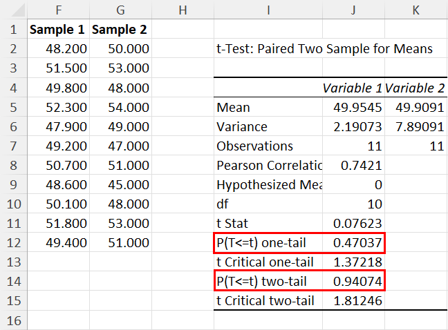
I’ve highlighted the cells in the above screenshot where you should find the p-values .

Find P-Value Using Excel VBA

Suppose, you find it challenging to remember various formula syntaxes and arguments of Excel functions. Or, you’d like to automate the task of finding the p-value using a programmatic method. In both scenarios, you can use Excel VBA.

You can create a VBA macro using the following script:

To learn the steps to create a VBA macro using a VBA script, read this Excel article now:

📒 Read More : How To Use The VBA Code You Find Online

The above script visually guides you to calculate p-values using the Z.TEST function.

You shall see the following prompts if you ruin the macro:

• Input box for the sample dataset

• Prompt for the population mean

• Input box for the population standard deviation

• Prompt for destination cell range

When you go through the above steps, Excel calculates the p-value in the selected cell.

If you wish to calculate the p-value with the t-Test, use the following script:

You just need to create a VBA macro using the above script.

Then, the VBA script input boxes shall visually guide you through the process.

⚠️ Warning : Excel VBA doesn’t allow the use of Excel undo features to revert back to the original workbook structure. So, create a backup copy of the workbook before running any VBA macros.

Conclusions

Before going through this Excel tutorial, if you thought calculating p-value in statistical analysis was a complex tax, your perception should have changed by now. So far, you must have learned that it’s pretty easy to find the p-value of a statistical experiment to disprove or establish a null hypothesis. All you need to do is follow the manual and automatic methods mentioned above.

Did the article help you to clear your doubts about p-value or probability value calculation in Excel? Comment below!

About the Author

Bipasha Nath

Subscribe for awesome Microsoft Excel videos 😃

John MacDougall

I’m John , and my goal is to help you Excel!

You’ll find a ton of awesome tips , tricks , tutorials , and templates here to help you save time and effort in your work.

• Pivot Table Tips and Tricks You Need to Know
• Everything You Need to Know About Excel Tables
• The Complete Guide to Power Query
• Introduction To Power Query M Code
• The Complete List of Keyboard Shortcuts in Microsoft Excel
• The Complete List of VBA Keyboard Shortcuts in Microsoft Excel

Related Posts

How To Find Z-Score in Excel

May 14, 2024

Learn how to find Z-score in Excel in this quick and easy-to-remember...

4 Ways to Calculate Weighted Average in Excel

Aug 14, 2023

You must be precise if you're analyzing data for actionable insights. Enter...

3 Ways to Calculate a Pearson’s Correlation Coefficient in Excel

Aug 23, 2020

Learn 3 easy ways to calculate the Pearson’s Correlation Coefficient statistic in Excel.

Submit a Comment Cancel reply

Your email address will not be published. Required fields are marked *

Save my name, email, and website in this browser for the next time I comment.

Submit Comment

This site uses Akismet to reduce spam. Learn how your comment data is processed .

Get the Latest Microsoft Excel Tips

Follow us to stay up to date with the latest in Microsoft Excel!

Machine Learning

Artificial Intelligence

Control System

Supervised Learning

Classification, miscellaneous, related tutorials.

Interview Questions

• Send your Feedback to [email protected]

Help Others, Please Share

Learn Latest Tutorials

Transact-SQL

Reinforcement Learning

R Programming

React Native

Python Design Patterns

Python Pillow

Python Turtle

Preparation

Verbal Ability

Company Questions

Trending Technologies

Cloud Computing

Data Science

B.Tech / MCA

Data Structures

Operating System

Computer Network

Compiler Design

Computer Organization

Discrete Mathematics

Ethical Hacking

Computer Graphics

Software Engineering

Web Technology

Cyber Security

C Programming

Data Mining

Data Warehouse

Thank you for visiting nature.com. You are using a browser version with limited support for CSS. To obtain the best experience, we recommend you use a more up to date browser (or turn off compatibility mode in Internet Explorer). In the meantime, to ensure continued support, we are displaying the site without styles and JavaScript.

• View all journals
• My Account Login
• Explore content
• About the journal
• Publish with us
• Sign up for alerts
• Open access
• Published: 16 May 2024

Geologically younger ecosystems are more dependent on soil biodiversity for supporting function

• Jiao Feng   ORCID: orcid.org/0000-0003-2879-3498 1 , 2 ,
• Yu-Rong Liu   ORCID: orcid.org/0000-0003-1112-4255 1 , 2 , 3 ,
• David Eldridge   ORCID: orcid.org/0000-0002-2191-486X 4 ,
• Qiaoyun Huang   ORCID: orcid.org/0000-0002-2733-8066 1 , 2 ,
• Wenfeng Tan   ORCID: orcid.org/0000-0002-3098-2928 2 , 3 &
• Manuel Delgado-Baquerizo   ORCID: orcid.org/0000-0002-6499-576X 5  

Nature Communications volume  15 , Article number:  4141 ( 2024 ) Cite this article

368 Accesses

4 Altmetric

Metrics details

• Biodiversity

Soil biodiversity contains the metabolic toolbox supporting organic matter decomposition and nutrient cycling in the soil. However, as soil develops over millions of years, the buildup of plant cover, soil carbon and microbial biomass may relax the dependence of soil functions on soil biodiversity. To test this hypothesis, we evaluate the within-site soil biodiversity and function relationships across 87 globally distributed ecosystems ranging in soil age from centuries to millennia. We found that within-site soil biodiversity and function relationship is negatively correlated with soil age, suggesting a stronger dependence of ecosystem functioning on soil biodiversity in geologically younger than older ecosystems. We further show that increases in plant cover, soil carbon and microbial biomass as ecosystems develop, particularly in wetter conditions, lessen the critical need of soil biodiversity to sustain function. Our work highlights the importance of soil biodiversity for supporting function in drier and geologically younger ecosystems with low microbial biomass.

Similar content being viewed by others

Severe decline in large farmland trees in India over the past decade

Land conversion to agriculture induces taxonomic homogenization of soil microbial communities globally

A climate-induced tree species bottleneck for forest management in Europe

Introduction.

Soil biodiversity is critical for the sustainability of multiple ecosystem functions such as nutrient cycling, organic matter decomposition, and plant production 1 , 2 , 3 . Thus, a growing number of studies have highlighted the pivotal role of soil biodiversity in supporting ecosystem functions from local to global scales and across ecosystems 3 , 4 , 5 . The mechanisms behind the biodiversity-ecosystem function (BEF) relationship are relatively intuitive: diverse soil biota can provide a broad array of functions that enable the complex depolymerization of organic matter, ultimately regulating the ingress of nutrients and energy into the soil ecosystem 3 , 4 . This may be particularly important in less productive (e.g., drylands) or early successional ecosystems wherein plant cover, soil organic carbon (C), microbial biomass and nutrient availability are low 6 , 7 , and ecosystem maintenance depends on the biodiversity-driven processes, including biological nitrogen (N) fixation, litter and organic matter decomposition and associated inputs of key soil resources 5 , 8 , 9 . However, the extent to which soil biodiversity supports critical ecosystem functions (i.e., soil BEF) might diminish with increasing ecosystem development, as a result of greater plant biomass production and larger pools of C and nutrients 7 , 10 . Moreover, changes in dominant soil taxa during ecosystem development 11 , 12 , which are known to influence essential soil functions 7 , 12 , 13 , could further suppress the positive soil BEF relationships. Thus, following millions of years of soil development (i.e., pedogenesis) or under conditions experienced in more productive ecosystems, soil function may become less dependent upon, and therefore decoupled from, soil biodiversity. Yet, how and why the contribution of soil biodiversity to ecosystem function changes as ecosystem develops remains virtually unknown.

Herein, we hypothesize that the fundamental role of soil biodiversity to support ecosystem functions (soil BEF) will be less important in older and more productive ecosystems versus younger and less productive ecosystems. The reason is that as ecosystems get old, they naturally accumulate organic matter having an important legacy of nutrients and C that can be recycled within the ecosystem. However, in low productive and in young ecosystems lacking biologically fixed elements such as nitrogen and C, biodiversity is essential to ensure the entrance of resources into the soil system. Assessing the contribution of soil biodiversity to regulating multiple ecosystem functions (multifunctionality) as ecosystem develops across wide environmental gradients is critical to better incorporate knowledge of soil microbial processes into Earth system models, and to identify areas for soil biodiversity conservation under future environmental changes.

To address these knowledge gaps, we investigated the changes in soil BEF relationships across 87 globally distributed sites along 16 soil chronosequences, ranging in age from centuries to millennia (Fig.  1A ; Supplementary Table  1 ). The datasets used in this study was retrieved from refs. 13 , 14 , 15 . This data has been previously used to understand the changes in soil biodiversity 13 , antibiotic resistance genes (ARGs) 15 , 16 and ecosystem properties 14 during ecosystem development. These soils come from different chronosequences with known soil ages 13 , offering a unique opportunity to evaluate the influence of pedogenesis on soil BEF relationships. For each study site, five composite soil samples containing information on soil biodiversity and functions were available. These samples were used to estimate the local correlation coefficients (Spearman) between soil biodiversity and function (local soil BEF relationships determined within each ecosystem) (Methods). In particular, we investigated the relationships between the diversity (richness) of four typical soil organisms (invertebrates, protists, fungi and bacteria) and multiple ecosystem functions related to water regulation, organic matter decomposition, mutualism, nutrient cycling, plant pathogen control, and ARGs control (Methods). Overall, the within-site chronosequences encompass a wide range of origins (volcanic, sedimentary, dunes, and glaciers), climatic conditions (tropical, temperate, continental, polar, and arid) and vegetation types (forests, shrublands, grasslands, and croplands). Various environmental factors, including spatial, climatic, plant, edaphic, and microbial factors, may also influence the linkages between soil biodiversity and ecosystem functions 12 , 13 . Our study simultaneously considered all of these factors using structural equation modeling (SEM) and mixed-effects meta-regression models to test hypotheses on the mechanistic relationships for soil BEF as ecosystem develops.

A Locations of the 16 soil chronosequences (from 87 globally distributed sites) included in this study (see refs. 13 , 14 , 15 for original details); B Patterns of within-site BEF relationships between multidiversity and multifunctionality; and C Values of BEF between multidiversity and ecosystem individual functions for soils of different age groups. The free continental data of the world map in ( A ) was sourced from Natural Earth, supported by the North American Cartographic Information Society ( https://www.naturalearthdata.com/ ). ArcGIS Desktop 10.8 (Esri, West Redlands, CA, USA) was employed for mapping the distribution of the study sites. Detailed information for the 16 chronossequences was shown in Supplementary Table  1 . The values (mean ± standard error (SE)) of BEF relationships were calculated using the Spearman rank correlations (Methods). Multidiversity represents averaging biodiversity of invertebrates, protists, fungi and bacteria. Averaged, T10, T25, T50, T75 and T90, represents within-site BEF relationship between multidiversity and multifunctionality quantified using averaged method and at threshold of 10%, 25%, 75% and 90%, respectively (Methods). The error bands surrounding the regression lines represent the 95% confidence interval of the correlation. The color of lines in ( B ) represents within-site soil BEF relationships between multidiversity and multifunctionality quantified using both averaged and threshold approaches. In ( C ), soils were classified into 6 groups ranging of age from hundreds (10 2 ) to millions (10 7 ) of years in a power series: Group 2, < 10 2 years, n  = 8 independent samples; Group 3, 10 2  ~ 10 3 years, n  = 18 independent samples; Group 4, 10 3  ~ 10 4 years, n  = 20 independent samples; Group 5, 10 4  ~ 10 5 years, n  = 15 independent samples; Group 6, 10 5  ~ 10 6 years, n  = 18 independent samples; Group 7, 10 6  ~ 10 7 years, n  = 8 independent samples. Ky, 1000 years; AMF Arbuscular Mycorrhizal fungi, ARGs antibiotic resistance genes. A two-sided test was used to assess the significance of the correlation analysis, with a threshold of P value < 0.05 (*) and < 0.01 (**), respectively. Exact P  value and source data are provided as a Source Data file.

Results and discussion

Our work provides valuable evidence that soil biodiversity is more important for supporting function in younger and less productive ecosystems. However, we also found a negative correlation between soil BEF and substrate age indicating that older ecosystems are less dependent on biodiversity to support function, probably as a consequence of the organic matter and microbial biomass reservoir built over millions of years of soil development. Our results are important to understand the natural history of soil BEF relationships, and better forecast under what environmental conditions soil biodiversity is especially important when supporting function.

Reduced within-site BEF relationships as soil develops

We first explored the distribution of our soil BEF data, and found that within-site soil BEF relationships generally follow a normal shape distribution according to Skewness, kurtosis, and Shapiro-Wilk analyses ( p  > 0.05; Supplementary Fig.  1 ; Supplementary Table  2 ). Results of linear mixed-effects model showed that within-site BEF relationship between multidiversity (the averaged richness of invertebrates, protists, fungi and bacteria) and averaging ecosystem multifunctionality 6 is negatively correlated with soil age (Fig.  1B ). This result accords with our hypothesis and suggests that the contribution of soil biodiversity to support functions wanes after millions of years of soil development. Similar reductions in soil BEF relationship were observed even when considering a range of independent multifunctionality indexes with multiple thresholds (multi-threshold multifunctionality, including >25%, >50%, >75% and >90% thresholds). Specifically, the steepest decline was observed at the threshold of 50% and 75% ( p  < 0.01), indicating that greater biodiversity tends to support a lower number of functions working at high levels. This multi-threshold approach effectively captures the number of functions while accounting for trade-offs and correlations among functions 17 , providing robust evidence for the importance of soil biodiversity in sustaining fundamental functions in younger soils, such as soil respiration, decomposition, and nutrient cycling working at high level of function. This aligns with the Odum’s ecological successional theory that species in the early stages of development exhibit broader niches. Consequently, in younger soils with lower soil biodiversity (Supplementary Fig.  2 ), the increase in species diversity contributes to more efficient resource utilization and facilitates the enhancement of multiple ecosystem functions. In well-established older soils, however, the contribution of soil biodiversity to support function may be less noticeable given the legacy of millions of years of organic matter and microbial biomass accumulation which can now feed the ecosystem with resources. Additionally, the higher soil biodiversity following organic matter accumulation may lead to functional redundancy of essential functions measured in this study, further contributing to the diminished soil BEF relationships in older soils 5 .

Moreover, the weakened soil BEF relationship with increasing soil age holds true when considering multiple individual functions supported by soil biodiversity, including soil respiration, Arbuscular Mycorrhizal fungi (AMF) mutualism, and water holding capacity (WHC) (Fig.  1C ). Collectively, these declines in within-site soil BEF relationships suggest that soil biodiversity plays a crucial role in maintaining measured fundamental functions in geographically younger ecosystems, regardless of multifunctionality operating at low or high levels. We acknowledge that, in our study, the choice of functions may influence the evaluation of soil BEF relationships. Therefore, we emphasize the necessity of incorporating variables targeting broader dimensions of ecosystem functions, such as biological N fixation, food production or policy (among many others), into the multifunctionality frameworks to reinforce the robustness of conclusions in this study. Nevertheless, this study provides an important case illustrating the relationship between soil biodiversity and multifunctionality during soil development by incorporating multiple fundamental ecosystem functions, including soil respiration, decomposition, nutrient cycling, water and climate regulation etc.

Ecological context as a driver of within-site soil BEF relationships

We then employed combined analyses of SEM and mixed-effects meta-regression model to gain a system-level understanding on the influence of multiple environmental factors including climate, soil age, plant, edaphic and microbial factors in driving local soil BEF relationship (Fig.  2A ; Supplementary Figs.  3 and 4 ). Of the multiple environmental variables assessed, our results revealed microbial biomass to be the most important driver, exhibiting negative correlations with soil BEF relationships, regardless of whether function was considered as an average or as independent multi-threshold multifunctionality (Fig.  2B ). Increased plant cover and litter inputs over millions of years of soil development promote soil organic C and nutrient availability, thereby fueling the production of microbial biomass 7 , 14 . Earth system models have consistently highlighted the role of microbial biomass in decomposition and organic matter mineralization through the regulation of extracellular enzyme production 18 . Consequently, as soil age increases, the necessity of soil biodiversity for supporting ecosystem function is speculated to diminish, indirectly through the promotion of plant cover, soil organic C, and ultimately microbial biomass (Fig.  2A ; Supplementary Fig.  5 ). According to the Odum’s theory on ecosystem succession, there is a shift from ecosystems where soil is constrained by the accumulation of soil C and nutrients to those with sufficient resources. We posit that this shift from the less productive (oligotrophic) to the more productive (eutrophic) establishes a resource buffer and releases the dependency of fundamental ecosystem functions, such as decomposition and nutrient cycling, on soil biodiversity in the older and well-developed soils 19 . Support for this proposition comes from the negative associations between soil organic C and soil BEF relationships (Fig.  2B ). Overall, our findings suggest that geographically younger soils exhibit a greater dependence on soil biodiversity to sustain ecosystem functions due to lower plant cover, soil organic C accumulation and microbial biomass production.

A Relative importance of soil age and different environmental factors (including microbial biomass, spatial, climatic, edaphic and plant attributes) regulating BEF relationships between multidiversity and multifunctionality using Structural equation model; and B Relationships of essential environmental factors with soil BEF relationships. Multidiversity represents averaging biodiversity of four groups of soil organisms, including invertebrates, protists, fungi and bacteria. Averaged, T10, T25, T50, T75 and T90, represents within-site BEF relationship between multidiversity and multifunctionality quantified using averaged method and at threshold of 10%, 25%, 75% and 90%, respectively (Methods). The color of lines in ( B ) represents within-site soil BEF relationships between multidiversity and multifunctionality quantified using both averaged and threshold approaches. MB, microbial biomass, the sum of phospholipid fatty acid (PLFA) of bacteria and fungi. SOC, soil organic C; MAT, mean annual temperature; MAP, mean annual precipitation. Structural equation model was constructed using the maximum likelihood analysis to estimate the direct and mediating effect. A two-sided test was used to assess the significance of the correlation analysis, with a threshold of P value < 0.05 (*) and < 0.01 (**), respectively. Exact P value and source data are provided as a Source Data file.

We further revealed that local soil BEF relationships are influenced by changes in climatic factors, with significant reductions in the relationship as mean annual precipitation (MAP) increases (Fig.  2B ). By shaping the spatial patterns of plant cover and organic resources accumulation 5 , 20 , MAP could indirectly influence the production of microbial biomass and thus the maintenance of ecosystem functions by soil biodiversity (Fig.  2A ; Supplementary Fig.  5 ). Specifically, the decline in local soil BEF relationship with increasing MAP suggests that drier ecosystems are more dependent on the complementary utilization of resources by diverse taxa than more mesic regions. Consistently, our results show that local soil BEF relationships remain relatively constant across chronosequences in drylands, but declined significantly with soil development in non-drylands (Supplementary Fig.  6 ). Specifically, local soil BEF relationships remain constant or even became increasingly tight along local chronosequences such as in Jornada Desert and Cojiri. Conversely, more negative soil BEF relationships are observed at later stages of chronosequences in non-drylands, such as in Alps, Taiwan and Hawaii (Supplementary Fig.  7 ). In drylands, soils may be weakly developed even when aged due to water restrictions on soil weathering, soil organic C accumulation and biomass production 20 , 21 . Therefore, the negative influence of soil age on BEF may be limited in these ecosystems with reduced soil development. In other words, these ecosystems rarely accumulate enough organic matter and soil microbial biomass to be independent from soil biodiversity. Other factors influencing soil development, such as parent material may also exerting confounding effects on the patterns of within-site soil BEF along chronosequences. However, results of linear mixed-effects model showed that the observed declining pattern of within-site soil BEF with increasing soil age still held true after accounting for the influence of the parent material (Fig.  1B ). These results collectively underscore the pronounced reliance of multiple ecosystem functions on soil biodiversity in drylands, despite extensive soil maturation over millions of years. The revelation of this dependency amidst anticipated climatic shifts is especially pertinent, considering the increasing aridity of dryland ecosystems worldwide 21 , 22 .

The BEF relationships between separate soil groups and multifunctionality with soil development is also likely linked to changes in plant cover, soil organic C and microbial biomass (Supplementary Figs.  8 – 12 ). For example, the BEF relationship between the richness of smaller prokaryotic bacteria and multifunctionality was negatively associated with microbial biomass (Supplementary Fig.  12 ), suggesting that the bacterial community may play a crucial role in sustaining multifunctionality in infertile, younger soils with low microbial biomass. This finding accords with previous studies highlighting the effectiveness of bacteria and bacterial-based energy channels in nutrient cycling and turnover, accounting for their relative dominance in the early stages of soil development 7 , 12 . Conversely, similar negative associations were absent when considering the local BEF relationships between larger eukaryotic soil groups, such as invertebrates and fungi, and multifunctionality (Supplementary Figs.  9 and 11 ). According to the Odum’s theory, the body size of species increased during ecosystem development, accompanied by a gradual shift in life-history from an R-strategy (characterized by fast growth) to the K-strategy, which have higher competitiveness in a stable environment. Invertebrates and fungal communities that consume complex phenolic macromolecules and detritus (e.g., plant litter), have been found to be increasingly favored in long-term chronosequences 11 , 12 , which could play essential roles in regulating the potential rates of multiple ecosystem processes. Accordingly, our study suggests a shift in the functional role of single soil groups in supporting ecosystem multifunctionality during long-term pedogenesis, highlighting the need for a multitrophic perspective when unravelling the drivers of soil BEF relationships under changing environmental conditions.

Effects of soil community composition shifts on within-site soil BEF

To gain further insights into the potential mechanisms underpinning changes in soil BEF relationships along soil chronosequences, we analyzed how shifts in the proportion of dominant taxa were associated with soil BEF relationships (Fig.  3 ). We found significant shifts in the community composition of soil organisms, including bacteria, fungi, protists and invertebrates, across chronosequences and in response to changes in plant cover, soil organic C and microbial biomass (Fig.  3A ). For instance, the proportion of larger soil invertebrates (e.g., Annelida, Nematoda, Platyhelminthes, and Tardigrada) increased significantly with increasing soil organic C and microbial biomass. These taxa are often winners under benign conditions 12 , 23 , and may control the rates of multiple ecosystem processes by comminuting large amounts of plant residues and regulating resource flows within the brown food web 4 . Supporting this notion, we found positive correlations between the proportion of these dominant invertebrates and multiple ecosystem individual functions, including organic matter decomposition, soil respiration, phosphorus (P) mineralization, nutrient availability, and water regulation (Fig.  3C ). Therefore, the promotion of these soil invertebrate taxa as soil ages may support multiple dimensions of individual functions, subsequently reducing the dependence of multifunctionality on biodiversity in older soils. In contrast, the proportion of Actinobacteria declined with increasing levels of soil organic C and microbial biomass, which showed positive correlations with local soil BEF relationships (Fig.  3B ). In well-established soils with high microbial biomass, the dominance and performance of Actinobacteria in driving local soil BEF may therefore diminish. These findings align with previous studies suggesting that the abundance of Actinobacteria has significant positive effects on multifunctionality under infertile conditions 10 , 24 . Thus, a high level of overall biodiversity may not necessarily contribute equally to all measured functions in older and more complex ecosystems. Instead, certain functions may become more dependent on specific compositions within the community. These results underscore the pivotal role of soil community composition in driving fundamental ecosystem functions in older soils. In particular, we highlight the importance of conserving micro-faunal taxa for the maintenance of ecosystem functioning within these well-established soils.

A Relationships between the proportions of dominant bacterial, fungal, protistan and invertebrate taxa and essential environmental factors along chronosequences; B Correlations of the proportion of dominant soil organisms on BEF between multidiversity and multifunctionality; and C Relationships between the proportion of dominant soil organisms and multiple dimensions of ecosystem functions. Averaged, T10, T25, T50, T75 and T90, represents within-site BEF relationship between multidiversity and multifunctionality quantified using averaged method and at threshold of 10%, 25%, 75% and 90%, respectively (Methods). The color of lines in ( B ) represents within-site soil BEF relationships between multidiversity and multifunctionality quantified using averaged and threshold methods. A two-sided test was used to assess the significance of the correlation analysis, with a threshold of P value < 0.05 (*) and < 0.01 (**), respectively. Exact P  value and source data are provided as a Source Data file.

Implications of within-site soil BEF shifts along chronosequences

Our work provides important insights into the dynamics of within-site soil BEF relationships during long-term soil development, and stresses that climate, plant cover, soil C and microbial biomass play dominant roles in driving the long-term trajectories of ecosystem functions provided by multidiversity across biomes (Fig.  4 ). Changes in other factors such as soil pH, soil texture, and microbial network traits may also contribute to the reductions in soil BEF relationships as soil develops (Supplementary Figs.  13 – 15 ). For example, long-term pedogenesis frequently results in increases of finer soil particles and soil acidification 7 , 25 . These processes could act as environmental filters, leading to the selection of microbes and invertebrates with similar niches and, subsequently, niche overlap among soil taxa 12 , 13 . Furthermore, these factors can influence the relationships between the biodiversity of individual microbial groups and specific functions, resulting in both synergistic and trade-off effects on BEF between multidiversity and multifunctionality (Supplementary Figs.  8 – 12 ).

Multidiversity represents averaging biodiversity of four groups of soil organisms, including invertebrates, protists, fungi and bacteria. Figure 4 Created with Biorender.com released under a Creative Commons Attribution-NonCommercial-NoDerivs 4.0 International license ( https://creativecommons.org/licenses/by-nc-nd/4.0/ ).

Additionally, it is essential to acknowledge that other undocumented factors operate at a local scale such as human activities (e.g., agriculture, deforestation), may also influence ecosystem succession and result in changes in soil BEF relationships. Importantly, disturbances of ecosystems can set back the development, causing a regression to early successional changes and leading to reductions in soil organic C and microbial biomass. Consequently, disturbances reducing soil organic matter and microbial biomass may rejuvenate the importance of soil biodiversity to support function. In our study, all locations were relatively undisturbed (with the exception of Taiwan) so future work is needed to delve further into this hypothesis. We further emphasize that for a more comprehensive understanding of the mechanisms driving soil BEF relationships during ecosystem development, it is crucial to simultaneously consider the successional trajectories of multiple factors, including disturbances in the local site and covariations in biotic and abiotic factors.

Collectively, our findings demonstrate the significant role of multidiversity in sustaining multifunctionality across various threshold demands and multiple individual functions in geographical younger and drier ecosystems. Additionally, we identified potential mechanisms underlying these findings. Specifically, plant cover, soil organic C, and microbial biomass, which increase as ecosystem age, appear to reduce the reliance of functions on soil biodiversity. Such findings are crucial as they enhance our understandings of how microbial processes regulate terrestrial ecosystem functioning under new climate regimes. Additionally, a deeper understanding of soil BEF relationships during soil development is relevant for improving model projections of Earth system models involved in biogeochemical cycles. Current models often lack explicit resolution of microbial processes over timescales, and only track the flows and mass balance of C and nutrients between different compartments of soil organic matter and microbial biomass 19 , 26 . Together, our work emphasizes the importance of multidiversity in sustaining ecosystem functioning, particularly in an increasingly drier and perturbed world.

Site information and sampling protocol

Data used in this study was mainly retrieved from refs. 13 , 14 , 15 , all associated with the same survey. In these references, a global standardized field survey was conducted along 16 soil chronosequences between 2016 and 2017, which spanning nine countries from six continents (Fig.  1 and Supplementary Table  1 ). Soil ages along the selected chronosequences ranged from centuries to millennia according to geological surveys, isotopic dating techniques or models. In each chronosequence, soils differ only in the time since soil formation, with other soil-forming factors (including climate, vegetation, parent material and topography) remaining relatively constant (Supplementary Table  1 ). Overall, these chronosequences covered a wide range of chronosequence origins (volcanic, sedimentary, dunes, and glaciers), climatic conditions (tropical, temperate, continental, polar, and arid) and vegetation types (forests, shrublands, grasslands, and croplands).

Soil samplings were carried out following a standardized protocol as described in Ref. 14 . In brief, a 50 m × 50 m plot was selected within each chronosequence stage, and then five composite surface (0-10 cm) soil samples were collected under the dominant vegetation types. Plot size was chosen to fully account for the spatial heterogeneity of different ecosystems (e.g., grasslands, shrublands and forests etc.). Plant cover and the number of perennial plant species (plant diversity) were surveyed and calculated. Following field surveys, soils were sieved in fields ( < 2 mm) and separated into two subsamples. One soil subsample was air-dried to analyze soil physical and chemical properties. The other subsample of the soil was frozen immediately at −20 °C for molecular biology analysis. Taken together, a total of 435 soil samples from 87 plots, 16 chronosequences were analyzed.

Methods of soil physical and biochemical analysis

Methodological information for these analyses is described in Ref. 14 . In brief, for all soil samples, soil pH, soil salinity, soil texture (% of clay+silt), soil organic C, total N, total P and soil available P were measured. These soil variables were selected, because they have been found to change along chronosequences 7 , 14 , and were associated with changes in soil community 25 , 27 , 28 . Soil pH was determined with a pH meter, in a 1:2.5 mass:volume soil and water suspension. Soil salinity was measured in an aqueous extract of saturated paste by a conductivity meter. Soil texture was analyzed using a hydrometer procedure. Soil organic C was determined by a colorimetric method after oxidation with potassium dichromate and sulfuric acid. Soil total N was analyzed using a CN analyzer (LECO CHN628 Series, LECO Corporation, St Joseph, MI, USA). Soil total P was measured using a digestion method with sulfuric acid (3h at 415 °C). Soil available P was determined using a colorimetric method after extraction with bicarbonate. The microbial biomass was expressed as the phospholipid fatty acids (PLFAs) extracted from freeze-dried soil samples 14 .

Methods of soil molecular analysis

Soil DNA extractions and sequencing was done as described in ref. 13 . Soil DNA was extracted from soil samples using the Powersoil® DNA Isolation Kit (MoBio Laboratories, Carlsbad, CA, USA) following the manufacturer’s instructions. To characterize the richness (number of phylotypes) of invertebrates, protists, fungi and bacteria, eukaryotic 18S rRNA and prokaryotic 16S rRNA genes were sequenced using Euk1391f/EukBr and 515F/806R pair sets 29 , 30 . Bioinformatic processing was performed using a combination of QIIME 31 , USEARCH 32 and UNOISE3 33 . Phylotypes (i.e., Operational Taxonomic Units; OTUs) were identified at the 100% identity level. The OTU abundance tables were rarefied at 300 (invertebrates via 18S rRNA gene), 800 (protists via 18S rRNA gene), 2000 (fungi via 18S rRNA gene) and 5000 (bacteria via 16S rRNA gene), respectively, to ensure even sampling depth within each group of soil organisms. Protists were defined as all eukaryotic taxa, except for fungi, invertebrates (Metazoa), and vascular plants (Streptophyta).

Soil biodiversity index calculation

The diversity (richness, i.e., number of phylotypes) of soil invertebrates, protists, fungi and bacteria was determined from rarefied OTU abundance tables. To obtain a quantitative index of soil biodiversity for each sample, the biodiversity traits of four groups of soil organisms (invertebrates, protists, fungi and bacteria) were combined by averaging the standardized scores (0-1 normalization) of diversity of all groups. This approach is commonly used to calculate multiple biodiversity indices (multidiversity) for soil and plant communities 6 , 34 .

Assessments of multiple ecosystem functions

This data was available from refs. 13 , 14 and 15 . In each plot, 13 proxies reflecting ecosystem functions, processes, or properties regulated by soil organisms and belonging to a wide range of potential ecosystem functions were included: water regulation (potential infiltration, water holding capacity), organic matter decomposition (soil respiration and extracellular enzyme activities related to lignin, chitin, sugar degradation and P mineralization), nutrient cycling (available N, available P), mutualism (Ectomycorrhizal fungi (EMF) and Arbuscular Mycorrhizal fungi (AMF) fungi), plant pathogens control (reduced relative abundance of fungal plant pathogens in soil) and ARGs control (reduced abundance of ARGs in soils).

Data methods are described in refs. 13 , 14 and 15 . In brief, the potential infiltration rate was measured by monitoring the time takes for a set amount of water to infiltrate through soil columns in the laboratory 35 . Soil water holding capacity was determined according to a saturation-drainage method 36 . The methods for available P were as described above. The availability of N (ammonium and nitrate) in soil was obtained by colorimetric assays after extracted using K 2 SO 4 extracts. The activities of extracellular enzymes, including β-glucosidase (sugar degradation), N-acetylglucosaminidase (chitin degradation) and phosphatase (P mineralization) were measured using fluorescence method 37 . Moreover, a MicroResp approach was used to measure lignin-induced respiration 38 . Soil respiration (the basal flux of CO 2 ) was estimated using an isotope approach by adding 13 C-glucose (99 atom% U-13C, Cambridge Isotope Laboratories) 39 . The relative abundances of EMF, AMF and potential fungal plant pathogens in soils were obtained from the amplicon sequencing analyses and were inferred by parsing the soil phylotypes using FUNguild 40 . ARGs were retrieved from ref. 15 , 16 . The total abundance of 285 unique ARGs encoding resistance to all of the major categories of antibiotics was obtained by the high throughput qPCR 41 . The inverse abundance of potential fungal plant pathogens and ARGs were obtained by calculating the inverse of the variables, respectively (×−1).

To obtain a quantitative index for multiple ecosystem functions, multifunctionality was calculated by two of the most commonly methods used: “averaging approach” and the “multiple threshold approach” 17 . The averaging approach was evaluated by calculating the mean values of all 13 standardized (0-1 normalization) ecosystem functional proxies. Threshold-based approach evaluates the total number of functions that exceed or equal to a predefined percentage of the maximum observed value of each individual function. Threshold-based multifunctionality (MF t ) was calculated using Eq. ( 1 ) 42 :

where F is the number of functions measured, f i represents the value for function i in a specific plot, r i represents a mathematical function that sets f i to be positive and t i is the threshold value corresponding to the predefined proportion of the maximum observed value for each function. Multiple threshold approach is commonly recommended, as the selection of a given threshold is arbitrary 17 , 34 . We used a set of threshold: 10%, 25%, 50%, 75% and 90% to represent multifunctionality that at low, medium, and high threshold of the observed maximum functioning.

Microbial co-occurrence network traits

Microbial co-occurrence network including soil invertebrates, protists, fungi and bacteria was constructed for each plot, respectively, in order to assess the effects of pedogenesis on the overall architecture and potential biotic linkages of soil biota. A total of 87 co-occurrence networks were obtained to represent each chronosequence stages. The networks were constructed based on Spearman’s correlation algorithm of the proportions of different phylotypes (OTUs). Specifically, networks were built and analyzed using the “WGCNA” and “igraph” R package. The nodes in the networks represent the taxonomic phylotypes of soil organisms, and the edges correspond to significant linkage between two nodes. A set of topological parameters were calculated to describe the biotic linkages of the networks, including the numbers of nodes and edges, positive and negative correlation numbers, average degree, graph density, degree centralization and modularity 43 .

Statistical analyses

The local soil BEF relationships were analyzed from multiple aspects: multidiversity vs. multifunctionality (both averaging approach and multiple threshold approach), biodiversity of separate groups of organisms (including invertebrates, protists, fungi and bacteria) vs. multifunctionality, and biodiversity of separate groups of organisms vs. individual ecosystem functions. In each plot, the spearman’s correlation coefficients were calculated to represent the local soil BEF relationships 44 , 45 . Specifically, the correlation analyses were conducted using “corrplo” R package. The resulting P  values were adjusted for multiple comparisons using the “fdr” method to control for the chance of false positives. Stronger positive correlation suggests higher capacity of soil biodiversity to promote ecosystem functions. The Skewness, kurtosis, and Shapiro-Wilk analyses were conducted to test the normality of local soil BEF relationships (Supplementary Fig.  1 ; Supplementary Table  2 ).

Linear mixed-effects model was employed to analyze the relationship of within-site soil BEF relationships between multidiversity and averaging ecosystem multifunctionality with soil age. In this model, the parent material, climatic conditions, vegetation type, and location were introduced as random factors using “nlme” R package. Moreover, soils were classified into 6 groups ranging of age from hundreds (10 2 ) to millions (10 7 ) of years, utilizing a power series based on soil ages provided in Supplementary Table  1 . For instance, age group 2 represents soils with age lower than 10 2 years, and age group 7 represents soils with age ranging between 10 6 and 10 7 years. Both linear and polynomial regression model were conducted to analyze the association between soil age groups and within-site soil BEF relationships. Furthermore, the association between soil age and BEF relationships were analyzed for drylands and non-dryland ecosystems, respectively. Drylands and non-drylands were classified according to Aridity Index (AI): drylands (AI < 0.50) and non-drylands (AI > 0.5) 13 .

We aimed to identify the best environmental variables as predictors of changes in BEF relationships during long-term pedogenesis. These environmental variables include multiple spatial (Distance equator), climatic (mean annual temperature, MAT; mean annual precipitation, MAP; mean diurnal range; precipitation seasonality, temperature seasonality), edaphic (soil texture, soil organic C, soil C:N ratio, soil pH, soil N:P, soil salinity), microbial biomass, plant (plant cover and plant richness) and microbial network traits (Node numbers, total edge numbers, positive edge numbers, negative edge numbers, average degree, degree centralization, graph density and modularity). Climatic data were obtained from WorldClim ( http://www.worldclim.org ) at a resolution of 1 km.

To achieve a system-level understanding of the potential major drivers for the local soil BEF relationships across spatial, time, edaphic and climatic gradients, a conceptual model was developed that could be further tested by SEM. The conceptual model was constructed according to previous knowledges (See Priori Model in Supplementary Fig.  3 ). We hypothesized that soil age, together with other important factors affecting pedogenesis such as climatic and biotic (including plant and microbial) attributes, may influence BEF relationships directly or indirectly by influencing edaphic variables and microbial biomass production 7 , 25 , 46 . The chi-squared test (χ 2 , the model has a good fit when χ 2 was low and the P -value > 0.05) and the root-mean-square error of approximation (RSMEA, the model has a good fit when 0 ≤ RMSEA ≤ 0.05) were conducted to test the overall goodness of SEM 47 , 48 . The SEM analysis was conducted by Amos 18.0 (IBM, SPSS, New York, USA).

Additionally, meta-analytic models were conducted to evaluate the combined effects of multiple environmental factors on within-site soil BEF relationships across chronosequences (Supplementary Fig.  4 ). Briefly, the mixed-effects meta-regression model was constructed by ‘glmulti’ package in R 49 . The importance of different factors was estimated according to the sum of Akaike weights. The weight was considered as the overall support for each variable in all potential models. A cutoff of 0.8 was set to identify the significant predictors for each model. Further, Pearson’s correlation analysis was used to analyze the relationships of different environmental factors with local BEF relationships along chronosequences. A two-sided test was used to assess the significance of the correlation, with a threshold of P  value < 0.05 and < 0.01, respectively.

Reporting summary

Further information on research design is available in the  Nature Portfolio Reporting Summary linked to this article.

Data availability

The raw data and processes data for all figures and supplementary materials in this study have been deposited in the figshare under accession code: https://figshare.com/s/7999a7433ec52638a05b . Additional figures and tables can be found in the Supporting Information. Original data was retrieved from refs. 13 , 14 and 15 .

Code availability

All code associated with our analyses in this study is available at https://figshare.com/s/746673e2b49ba9374273 .

van Elsas, J. D. et al. Microbial diversity determines the invasion of soil by a bacterial pathogen. Proc. Natl Acad. Sci. 109 , 1159–1164 (2012).

Article   ADS   PubMed   PubMed Central   Google Scholar  

Bardgett, R. D. & van der Putten, W. H. Belowground biodiversity and ecosystem functioning. Nature 515 , 505–511 (2014).

Article   ADS   CAS   PubMed   Google Scholar  

Wagg, C., Bender, S. F., Widmer, F. & van der Heijden, M. G. A. Soil biodiversity and soil community composition determine ecosystem multifunctionality. Proc. Natl Acad. Sci. 111 , 5266–5270 (2014).

Article   ADS   CAS   PubMed   PubMed Central   Google Scholar  

Delgado-Baquerizo, M. et al. Multiple elements of soil biodiversity drive ecosystem functions across biomes. Nat. Ecol. Evol. 4 , 210–220 (2020).

Article   PubMed   Google Scholar  

Hu, W. et al. Aridity-driven shift in biodiversity–soil multifunctionality relationships. Nat. Commun. 12 , 5350 (2021).

Maestre, F. T. et al. Plant species richness and ecosystem multifunctionality in global drylands. Science 335 , 214–218 (2012).

Turner, B. L. et al. Contrasting patterns of plant and microbial diversity during long-term ecosystem development. J. Ecol. 107 , 606–621 (2019).

Article   CAS   Google Scholar  

Grime, J. P. Biodiversity and ecosystem function: the debate deepens. Science 277 , 1260–1261 (1997).

Grime, J. P. Benefits of plant diversity to ecosystems: immediate, filter and founder effects. J. Ecol. 86 , 902–910 (1998).

Article   Google Scholar  

Trivedi, P., Anderson, I. C. & Singh, B. K. Microbial modulators of soil carbon storage: integrating genomic and metabolic knowledge for global prediction. Trends Microbiol . 21 , 641–651 (2013).

Article   CAS   PubMed   Google Scholar  

Bastian, F., Bouziri, L., Nicolardot, B. & Ranjard, L. Impact of wheat straw decomposition on successional patterns of soil microbial community structure. Soil Biol. Biochem. 41 , 262–275 (2009).

Williamson, W. M., Wardle, D. A. & Yeates, G. W. Changes in soil microbial and nematode communities during ecosystem decline across a long-term chronosequence. Soil Biol. Biochem. 37 , 1289–1301 (2005).

Delgado-Baquerizo, M. et al. Changes in belowground biodiversity during ecosystem development. Proc. Natl Acad. Sci. 116 , 6891–6896 (2019).

Delgado-Baquerizo, M. et al. The influence of soil age on ecosystem structure and function across biomes. Nat. Commun. 11 , 4721 (2020).

Chen, Q.-L. et al. Cross-biome antibiotic resistance decays after millions of years of soil development. ISME J. 16 , 1864–1867 (2022).

Article   PubMed   PubMed Central   Google Scholar  

Delgado-Baquerizo, M. et al. The global distribution and environmental drivers of the soil antibiotic resistome. Microbiome 10 , 219 (2022).

Byrnes, J. E. K. et al. Investigating the relationship between biodiversity and ecosystem multifunctionality: challenges and solutions. Methods Ecol. Evol . 5 , 111124 (2014).

Wang, G., Post, W. M. & Mayes, M. A. Development of microbial-enzyme-mediated decomposition model parameters through steady-state and dynamic analyses. Ecol. Appl. 23 , 255–272 (2013).

Sokol, N. W. et al. Life and death in the soil microbiome: how ecological processes influence biogeochemistry. Nat. Rev. Microbiol. 20 , 415–430 (2022).

Feng, J. et al. Phosphorus transformations along a large‐scale climosequence in arid and semi‐arid grasslands of northern China. Glob. Biogeochem. Cy. 30 , 1264–1275 (2016).

Article   ADS   CAS   Google Scholar  

Wang, L. et al. Dryland productivity under a changing climate. Nat. Clim. Change 12 , 981–994 (2022).

Article   ADS   Google Scholar  

Delgado-Baquerizo, M. et al. Decoupling of soil nutrient cycles as a function of aridity in global drylands. Nature 502 , 672–676 (2013).

Doblas-Miranda, E., Wardle, D. A., Peltzer, D. A. & Yeates, G. W. Changes in the community structure and diversity of soil invertebrates across the Franz Josef Glacier chronosequence. Soil Biol. Biochem. 40 , 1069–1081 (2008).

Delgado-Baquerizo, M. et al. Microbial richness and composition independently drive soil multifunctionality. Funct. Ecol. 31 , 2330–2343 (2017).

Laliberté, E. et al. Experimental assessment of nutrient limitation along a 2-million-year dune chronosequence in the south-western Australia biodiversity hotspot. J. Ecol. 100 , 631–642 (2012).

Sierra, C. A. & Müller, M. A general mathematical framework for representing soil organic matter dynamics. Ecol. Monogr. 85 , 505–524 (2015).

Fierer, N. & Jackson, R. B. The diversity and biogeography of soil bacterial communities. Proc. Natl Acad. Sci. 103 , 626–631 (2006).

Fierer, N. Embracing the unknown: disentangling the complexities of the soil microbiome. Nat. Rev. Microbiol. 15 , 579–590 (2017).

Ramirez, K. S. et al. Biogeographic patterns in below-ground diversity in New York City’s Central Park are similar to those observed globally. Proc. Biol. Sci. 281 , 20141988 (2014).

PubMed   PubMed Central   Google Scholar  

Hirakata, Y. et al. Temporal variation of eukaryotic community structures in UASB reactor treating domestic sewage as revealed by 18S rRNA gene sequencing. Sci. Rep. 9 , 12783 (2019).

Caporaso, J. G. et al. QIIME allows analysis of high-throughput community sequencing data. Nat. Methods 7 , 335–336 (2010).

Article   CAS   PubMed   PubMed Central   Google Scholar  

Edgar, R. C. UPARSE: highly accurate OTU sequences from microbial amplicon reads. Nat. Methods 10 , 996–998 (2013).

Fitzpatrick, A. H. et al. Benchmarking bioinformatic tools for amplicon-based sequencing of norovirus. Appl. Environ. Microbiol . 89 , e0152222 (2023).

Schuldt, A. et al. Biodiversity across trophic levels drives multifunctionality in highly diverse forests. Nat. Commun. 9 , 2989 (2018).

Peter, K. D. & Ries, J. B. Infiltration rates affected by land levelling measures in the Souss valley, South Morocco. Z. Geomorphol. 57 , 59–72 (2013).

Verheijen, F. G. A. et al. The influence of biochar particle size and concentration on bulk density and maximum water holding capacity of sandy vs sandy loam soil in a column experiment. Geoderma 347 , 194–202 (2019).

Marx, M.-C., Wood, M. & Jarvis, S. A microplate fluorimetric assay for the study of enzyme diversity in soils. Soil Biol. Biochem. 33 , 1633–1640 (2001).

Campbell, C. D., Chapman, S. J., Cameron, C. M., Davidson, M. S. & Potts, J. M. A rapid microtiter plate method to measure carbon dioxide evolved from carbon substrate amendments so as to determine the physiological profiles of soil microbial communities by using whole soil. Appl. Environ. Microbiol. 69 , 3593–3599 (2003).

Derrien, D. et al. Does the addition of labile substrate destabilise old soil organic matter? Soil Biol. Biochem. 76 , 149–160 (2014).

Nguyen, N. H. et al. FUNGuild: An open annotation tool for parsing fungal community datasets by ecological guild. Fungal Ecol. 20 , 241–248 (2016).

Hu, H.-W. et al. Diversity of herbaceous plants and bacterial communities regulates soil resistome across forest biomes. Environ. Microbiol. 20 , 3186–3200 (2018).

Fanin, N. et al. Consistent effects of biodiversity loss on multifunctionality across contrasting ecosystems. Nat. Ecol. Evol. 2 , 269–278 (2018).

Assenov, Y., Ramírez, F., Schelhorn, S. E., Lengauer, T. & Albrecht, M. Computing topological parameters of biological networks. Bioinformatics 24 , 282–284 (2008).

van der Plas, F. et al. Biotic homogenization can decrease landscape-scale forest multifunctionality. Proc. Natl Acad. Sci. 113 , 3557–3562 (2016).

Ochoa-Hueso, R., Plaza, C., Moreno-Jiménez, E. & Delgado-Baquerizo, M. Soil element coupling is driven by ecological context and atomic mass. Ecol. Lett. 24 , 319–326 (2021).

Pichon N. A. et al. Nitrogen availability and plant functional composition modify biodiversity-multifunctionality relationships. Ecol. Lett. 27 , e14361 (2024).

Grace J. B. Structural equation modeling and natural systems . (Cambridge University Press, 2006).

Schermelleh-engel, K., Moosbrugger, H. & Müller, H. Evaluating the fit of structural equation models: tests of significance and descriptive goodness-of-fit measures. Method Psychol. Res. 8 , 23–74 (2003).

Google Scholar  

Calcagno, V. & de Mazancourt, C. glmulti: An R package for easy automated model selection with (Generalized) Linear Models. J. Stat. Softw. 34 , 1–29 (2010).

Download references

Acknowledgements

Wenfeng Tan was supported by the National Key Research and Development Program of China (2021YFD1901205). Jiao Feng was supported by the National Natural Science Foundation of China (32071595) and the Fundamental Research Funds for the Central Universities (2662023PY010). Yu-Rong Liu was supported by the National Natural Science Foundation of China (42177022). Manuel Delgado-Baquerizo acknowledges support from the Spanish Ministry of Science and Innovation (PID2020-115813RA-I00), and a project of the Fondo Europeo de Desarrollo Regional (FEDER) and the Consejería de Transformación Económica, Industria, Conocimiento y Universidades of the Junta de Andalucía (FEDER Andalucía 2014-2020 Objetivo temático “01 - Refuerzo de la investigación, el desarrollo tecnológico y la innovación”) associated with the research project P20_00879 (ANDABIOMA).

Author information

Authors and affiliations.

National Key Laboratory of Agricultural Microbiology, Huazhong Agricultural University, Wuhan, 430070, China

Jiao Feng, Yu-Rong Liu & Qiaoyun Huang

College of Resources and Environment, Huazhong Agricultural University, Wuhan, 430070, China

Jiao Feng, Yu-Rong Liu, Qiaoyun Huang & Wenfeng Tan

State Environmental Protection Key Laboratory of Soil Health and Green Remediation and Hubei Key Laboratory of Soil Environment and Pollution Remediation, Huazhong Agricultural University, Wuhan, 430070, China

Yu-Rong Liu & Wenfeng Tan

Centre for Ecosystem Science, School of Biological, Earth and Environmental Sciences, University of New South Wales, Sydney, NSW 2052, Australia

David Eldridge

Laboratorio de Biodiversidad y Funcionamiento Ecosistémico. Instituto de Recursos Naturales y Agrobiología de Sevilla (IRNAS), CSIC, Av. Reina Mercedes 10, E-41012, Sevilla, Spain

Manuel Delgado-Baquerizo

You can also search for this author in PubMed   Google Scholar

Contributions

M.D-B. and Y-R.L. developed the original ideas presented in the manuscript. J.F. and Y-R.L. analyzed the data. J.F. wrote the first draft of the paper. M.D-B., Y-R.L., D.E., Q.H. and W.T. edited the paper. All authors reviewed the paper and approved the final version of the manuscript.

Corresponding authors

Correspondence to Yu-Rong Liu or Manuel Delgado-Baquerizo .

Ethics declarations

Competing interests.

The authors declare no competing interests.

Peer review

Peer review information.

Nature Communications thanks Mirjam Pulleman, Weiming Yan and the other, anonymous, reviewer for their contribution to the peer review of this work. A peer review file is available.

Additional information

Publisher’s note Springer Nature remains neutral with regard to jurisdictional claims in published maps and institutional affiliations.

Supplementary information

Supplementary information, peer review file, reporting summary, rights and permissions.

Open Access This article is licensed under a Creative Commons Attribution 4.0 International License, which permits use, sharing, adaptation, distribution and reproduction in any medium or format, as long as you give appropriate credit to the original author(s) and the source, provide a link to the Creative Commons licence, and indicate if changes were made. The images or other third party material in this article are included in the article’s Creative Commons licence, unless indicated otherwise in a credit line to the material. If material is not included in the article’s Creative Commons licence and your intended use is not permitted by statutory regulation or exceeds the permitted use, you will need to obtain permission directly from the copyright holder. To view a copy of this licence, visit http://creativecommons.org/licenses/by/4.0/ .

Reprints and permissions

About this article

Cite this article.

Feng, J., Liu, YR., Eldridge, D. et al. Geologically younger ecosystems are more dependent on soil biodiversity for supporting function. Nat Commun 15 , 4141 (2024). https://doi.org/10.1038/s41467-024-48289-y

Download citation

Received : 14 October 2023

Accepted : 26 April 2024

Published : 16 May 2024

DOI : https://doi.org/10.1038/s41467-024-48289-y

Share this article

Anyone you share the following link with will be able to read this content:

Sorry, a shareable link is not currently available for this article.

Provided by the Springer Nature SharedIt content-sharing initiative

By submitting a comment you agree to abide by our Terms and Community Guidelines . If you find something abusive or that does not comply with our terms or guidelines please flag it as inappropriate.

Quick links

• Explore articles by subject
• Guide to authors
• Editorial policies

Sign up for the Nature Briefing newsletter — what matters in science, free to your inbox daily.