expression vector assignment

• school Campus Bookshelves
• menu_book Bookshelves
• perm_media Learning Objects
• login Login
• how_to_reg Request Instructor Account
• hub Instructor Commons

Margin Size

• Download Page (PDF)
• Download Full Book (PDF)
• Periodic Table
• Physics Constants
• Scientific Calculator
• Reference & Cite
• Tools expand_more
• Readability

selected template will load here

This action is not available.

7.14D: Shuttle Vectors and Expression Vectors

• Last updated
• Save as PDF
• Page ID 9321

\( \newcommand{\vecs}[1]{\overset { \scriptstyle \rightharpoonup} {\mathbf{#1}} } \)

\( \newcommand{\vecd}[1]{\overset{-\!-\!\rightharpoonup}{\vphantom{a}\smash {#1}}} \)

\( \newcommand{\id}{\mathrm{id}}\) \( \newcommand{\Span}{\mathrm{span}}\)

( \newcommand{\kernel}{\mathrm{null}\,}\) \( \newcommand{\range}{\mathrm{range}\,}\)

\( \newcommand{\RealPart}{\mathrm{Re}}\) \( \newcommand{\ImaginaryPart}{\mathrm{Im}}\)

\( \newcommand{\Argument}{\mathrm{Arg}}\) \( \newcommand{\norm}[1]{\| #1 \|}\)

\( \newcommand{\inner}[2]{\langle #1, #2 \rangle}\)

\( \newcommand{\Span}{\mathrm{span}}\)

\( \newcommand{\id}{\mathrm{id}}\)

\( \newcommand{\kernel}{\mathrm{null}\,}\)

\( \newcommand{\range}{\mathrm{range}\,}\)

\( \newcommand{\RealPart}{\mathrm{Re}}\)

\( \newcommand{\ImaginaryPart}{\mathrm{Im}}\)

\( \newcommand{\Argument}{\mathrm{Arg}}\)

\( \newcommand{\norm}[1]{\| #1 \|}\)

\( \newcommand{\Span}{\mathrm{span}}\) \( \newcommand{\AA}{\unicode[.8,0]{x212B}}\)

\( \newcommand{\vectorA}[1]{\vec{#1}}      % arrow\)

\( \newcommand{\vectorAt}[1]{\vec{\text{#1}}}      % arrow\)

\( \newcommand{\vectorB}[1]{\overset { \scriptstyle \rightharpoonup} {\mathbf{#1}} } \)

\( \newcommand{\vectorC}[1]{\textbf{#1}} \)

\( \newcommand{\vectorD}[1]{\overrightarrow{#1}} \)

\( \newcommand{\vectorDt}[1]{\overrightarrow{\text{#1}}} \)

\( \newcommand{\vectE}[1]{\overset{-\!-\!\rightharpoonup}{\vphantom{a}\smash{\mathbf {#1}}}} \)

An expression vector is generally a plasmid that is used to introduce a specific gene into a target cell.

LEARNING OBJECTIVES

Explain the structure and function of shuttle and expression vectors

Key Takeaways

• The plasmid is frequently engineered to contain regulatory sequences that act as enhancer and promoter regions and lead to efficient transcription of the gene carried on the expression vector.
• Expression vectors must have expression signals such as a strong promoter, a strong termination codon, adjustment of the distance between the promoter and the cloned gene, and the insertion of a transcription termination sequence and a portable translation initiation sequence.
• Expression vectors are used for molecular biology techniques such as site-directed mutagenesis.
• plasmid : A circle of double-stranded DNA that is separate from the chromosomes, which is found in bacteria and protozoa.
• expression vector : An expression vector, otherwise known as an expression construct, is generally a plasmid that is used to introduce a specific gene into a target cell.
• transcription : The synthesis of RNA under the direction of DNA.

An expression vector, otherwise known as an expression construct, is generally a plasmid that is used to introduce a specific gene into a target cell. Once the expression vector is inside the cell, the protein that is encoded by the gene is produced by the cellular-transcription and translation machinery ribosomal complexes. The plasmid is frequently engineered to contain regulatory sequences that act as enhancer and promoter regions and lead to efficient transcription of the gene carried on the expression vector. The goal of a well-designed expression vector is the production of large amounts of stable messenger RNA, and in extension, proteins. Expression vectors are basic tools for biotechnology and the production of proteins such as insulin, which is important for the treatment of diabetes.

After expression of the gene product, the purification of the protein is required; but since the vector is introduced to a host cell, the protein of interest should be purified from the proteins of the host cell. Therefore, to make the purification process easy, the cloned gene should have a tag. This tag could be histidine (His) tag or any other marker peptide.

Expression vectors are used for molecular biology techniques such as site-directed mutagenesis. Cloning vectors, which are very similar to expression vectors, involve the same process of introducing a new gene into a plasmid, but the plasmid is then added into bacteria for replication purposes. In general, DNA vectors that are used in many molecular-biology gene-cloning experiments need not result in the expression of a protein.

Expression vectors must have expression signals such as a strong promoter, a strong termination codon, adjustment of the distance between the promoter and the cloned gene, and the insertion of a transcription termination sequence and a PTIS (portable translation initiation sequence).

A shuttle vector is a vector that can propagate in two different host species, hence, inserted DNA can be tested or manipulated in two different cell types. The main advantage of these vectors is that they can be manipulated in E. coli and then used in a system which is more difficult or slower to use.

Shuttle vectors can be used in both eukaryotes and prokaryotes. Shuttle vectors are frequently used to quickly make multiple copies of the gene in E. coli (amplification). They can also be used for in vitro experiments and modifications such as mutagenesis and PCR. One of the most common types of shuttle vectors is the yeast shuttle vector that contains components allowing for the replication and selection in both E. coli cells and yeast cells. The E. coli component of a yeast shuttle vector includes an origin of replication and a selectable marker, such as an antibiotic resistance like beta lactamase. The yeast component of a yeast shuttle vector includes an autonomously replicating sequence (ARS), a yeast centromere (CEN), and a yeast selectable marker.

PRDV420: Introduction to R Programming

Vectors and Simple Manipulations

This section introduces the basic operations on vectors, most of which are done element-wise. Please pay attention to the recycling of vectors (usually, recycling doesn't generate an error or a warning, so it is easy to miss if it was unintended), missing values (NA), and logical vectors often used for data subsetting.

Vectors and assignment

R operates on named data structures . The simplest such structure is the numeric vector , which is a single entity consisting of an ordered collection of numbers. To set up a vector named x , say, consisting of five numbers, namely 10.4, 5.6, 3.1, 6.4 and 21.7, use the R command

This is an assignment statement using the function c() which in this context can take an arbitrary number of vector arguments and whose value is a vector got by concatenating its arguments end to end.

A number occurring by itself in an expression is taken as a vector of length one.

Notice that the assignment operator (' <- '), which consists of the two characters ' < ' ("less than") and ' - ' ("minus") occurring strictly side-by-side and it 'points' to the object receiving the value of the expression. In most contexts the ' = ' operator can be used as an alternative.

Assignment can also be made using the function assign() . An equivalent way of making the same assignment as above is with:

The usual operator, <- , can be thought of as a syntactic short-cut to this.

Assignments can also be made in the other direction, using the obvious change in the assignment operator. So the same assignment could be made using

If an expression is used as a complete command, the value is printed and lost . So now if we were to use the command

the reciprocals of the five values would be printed at the terminal (and the value of x , of course, unchanged).

The further assignment

would create a vector y with 11 entries consisting of two copies of x with a zero in the middle place.

Description

The templated class vector<T, A> is the base container adaptor for dense vectors. For a n -dimensional vector and 0 <= i < n every element v i is mapped to the i- th element of the container.

Defined in the header vector.hpp.

Template parameters

Type requirements.

None, except for those imposed by the requirements of Vector .

Public base classes

vector_expression<vector<T, A> >

[1] Supported parameters for the adapted array are unbounded_array<T> , bounded_array<T> and std::vector<T> .

Unit Vector

The templated class unit_vector<T> represents canonical unit vectors. For the k -th n -dimensional canonical unit vector and 0 <= i < n holds u k i = 0 , if i <> k , and u k i = 1 .

Vector Expression .

None, except for those imposed by the requirements of Vector Expression .

vector_expression<unit_vector<T> >

Zero Vector

The templated class zero_vector<T> represents zero vectors. For a n -dimensional zero vector and 0 <= i < n holds z i = 0 .

vector_expression<zero_vector<T> >

Scalar Vector

The templated class scalar_vector<T> represents scalar vectors. For a n -dimensional scalar vector and 0 <= i < n holds z i = s .

vector_expression<scalar_vector<T> >

Copyright (©) 2000-2002 Joerg Walter, Mathias Koch Permission to copy, use, modify, sell and distribute this document is granted provided this copyright notice appears in all copies. This document is provided ``as is'' without express or implied warranty, and with no claim as to its suitability for any purpose.

Last revised: 1/15/2003

Expression vector

Definition noun, plural: expression vectors A plasmid containing the required regulatory sequences specifically used for the expression of a particular gene into proteins within the target cell . Supplement The expression vector is a plasmid engineered to introduce a particular gene into the target cell . The plasmid contains the regulatory sequences that serve as enhancer and promoter regions needed for the expression of a specific gene using the transcription and translation machinery of the target cell . An example of expression vector is the plasmid used to produce insulin important for treating diseases such as diabetes . Another example is the expression vector that introduces specific genes necessary for the synthesis of beta-carotene into the cells of rice plants , giving rise to a new variety called golden rice. Synonym(s):

• expression construct

Related term(s):

• Mammalian expression vector

Last updated on July 21st, 2021

You will also like...

Genetics – Lesson Outline & Worksheets

  Topics Modules Quizzes/Worksheets Description Introduction to Genetics Genetics – Definition: Heredity and ..

Human Reproduction

Humans are capable of only one mode of reproduction, i.e. sexual reproduction. Haploid sex cells (gametes) are produced ..

Chemical Composition of the Body

The body is comprised of different elements with hydrogen, oxygen, carbon, and nitrogen as the major four. This tutorial..

Cell Structure

A typical eukaryotic cell is comprised of cytoplasm with different organelles, such as nucleus, endoplasmic reticulum, G..

Genetics and Evolution

Humans are diploid creatures. This means that for every chromosome in the body, there is another one to match it. Howeve..

Human Neurology

Human Neurology deals essentially with the nervous system of humans. It also features the various theories put forward b..

Related Articles...

No related articles found

2   Simple manipulations; numbers and vectors

2.1 vectors and assignment.

R operates on named data structures . The simplest such structure is the numeric vector , which is a single entity consisting of an ordered collection of numbers. To set up a vector named x , say, consisting of five numbers, namely 10.4, 5.6, 3.1, 6.4 and 21.7, use the R command

This is an assignment statement using the function c() which in this context can take an arbitrary number of vector arguments and whose value is a vector got by concatenating its arguments end to end. 1

1  With other than vector types of argument, such as list mode arguments, the action of c() is rather different. See Concatenating lists .

A number occurring by itself in an expression is taken as a vector of length one.

Notice that the assignment operator ( <- ), which consists of the two characters < (“less than”) and - (“minus”) occurring strictly side-by-side and it ‘points’ to the object receiving the value of the expression. In most contexts the = operator can be used as an alternative.

Assignment can also be made using the function assign() . An equivalent way of making the same assignment as above is with:

The usual operator, <- , can be thought of as a syntactic short-cut to this.

Assignments can also be made in the other direction, using the obvious change in the assignment operator. So the same assignment could be made using

If an expression is used as a complete command, the value is printed and lost 2 . So now if we were to use the command

2  Actually, it is still available as .Last.value before any other statements are executed.

the reciprocals of the five values would be printed at the terminal (and the value of x , of course, unchanged).

The further assignment

would create a vector y with 11 entries consisting of two copies of x with a zero in the middle place.

2.2 Vector arithmetic

Vectors can be used in arithmetic expressions, in which case the operations are performed element by element. Vectors occurring in the same expression need not all be of the same length. If they are not, the value of the expression is a vector with the same length as the longest vector which occurs in the expression. Shorter vectors in the expression are recycled as often as need be (perhaps fractionally) until they match the length of the longest vector. In particular a constant is simply repeated. So with the above assignments the command

generates a new vector v of length 11 constructed by adding together, element by element, 2*x repeated 2.2 times, y repeated just once, and 1 repeated 11 times.

The elementary arithmetic operators are the usual + , - , * , / and ^ for raising to a power. In addition all of the common arithmetic functions are available. log , exp , sin , cos , tan , sqrt , and so on, all have their usual meaning. max and min select the largest and smallest elements of a vector respectively. range is a function whose value is a vector of length two, namely c(min(x), max(x)) . length(x) is the number of elements in x , sum(x) gives the total of the elements in x , and prod(x) their product.

Two statistical functions are mean(x) which calculates the sample mean, which is the same as sum(x)/length(x) , and var(x) which gives

or sample variance. If the argument to var() is an n -by- p matrix the value is a p -by- p sample covariance matrix got by regarding the rows as independent p -variate sample vectors.

sort(x) returns a vector of the same size as x with the elements arranged in increasing order; however there are other more flexible sorting facilities available (see order() or sort.list() which produce a permutation to do the sorting).

Note that max and min select the largest and smallest values in their arguments, even if they are given several vectors. The parallel maximum and minimum functions pmax and pmin return a vector (of length equal to their longest argument) that contains in each element the largest (smallest) element in that position in any of the input vectors.

For most purposes the user will not be concerned if the “numbers” in a numeric vector are integers, reals or even complex. Internally calculations are done as double precision real numbers, or double precision complex numbers if the input data are complex.

To work with complex numbers, supply an explicit complex part. Thus

will give NaN and a warning, but

will do the computations as complex numbers.

2.3 Generating regular sequences

R has a number of facilities for generating commonly used sequences of numbers. For example 1:30 is the vector c(1, 2, ..., 29, 30) . The colon operator has high priority within an expression, so, for example 2*1:15 is the vector c(2, 4, ..., 28, 30) . Put n <- 10 and compare the sequences 1:n-1 and 1:(n-1) .

The construction 30:1 may be used to generate a sequence backwards.

The function seq() is a more general facility for generating sequences. It has five arguments, only some of which may be specified in any one call. The first two arguments, if given, specify the beginning and end of the sequence, and if these are the only two arguments given the result is the same as the colon operator. That is seq(2,10) is the same vector as 2:10 .

Arguments to seq() , and to many other R functions, can also be given in named form, in which case the order in which they appear is irrelevant. The first two arguments may be named from=value and to=value ; thus seq(1,30) , seq(from=1, to=30) and seq(to=30, from=1) are all the same as 1:30 . The next two arguments to seq() may be named by=value and length=value , which specify a step size and a length for the sequence respectively. If neither of these is given, the default by=1 is assumed.

For example

generates in s3 the vector c(-5.0, -4.8, -4.6, ..., 4.6, 4.8, 5.0) . Similarly

generates the same vector in s4 .

The fifth argument may be named along=vector , which is normally used as the only argument to create the sequence 1, 2, ..., length(vector) , or the empty sequence if the vector is empty (as it can be).

A related function is rep() which can be used for replicating an object in various complicated ways. The simplest form is

which will put five copies of x end-to-end in s5 . Another useful version is

which repeats each element of x five times before moving on to the next.

2.4 Logical vectors

As well as numerical vectors, R allows manipulation of logical quantities. The elements of a logical vector can have the values TRUE , FALSE , and NA (for “not available”, see below). The first two are often abbreviated as T and F , respectively. Note however that T and F are just variables which are set to TRUE and FALSE by default, but are not reserved words and hence can be overwritten by the user. Hence, you should always use TRUE and FALSE .

Logical vectors are generated by conditions . For example

sets temp as a vector of the same length as x with values FALSE corresponding to elements of x where the condition is not met and TRUE where it is.

The logical operators are < , <= , > , >= , == for exact equality and != for inequality. In addition if c1 and c2 are logical expressions, then c1 & c2 is their intersection ( “and” ), c1 | c2 is their union ( “or” ), and !c1 is the negation of c1 .

Logical vectors may be used in ordinary arithmetic, in which case they are coerced into numeric vectors, FALSE becoming 0 and TRUE becoming 1 . However there are situations where logical vectors and their coerced numeric counterparts are not equivalent, for example see the next subsection.

2.5 Missing values

In some cases the components of a vector may not be completely known. When an element or value is “not available” or a “missing value” in the statistical sense, a place within a vector may be reserved for it by assigning it the special value NA . In general any operation on an NA becomes an NA . The motivation for this rule is simply that if the specification of an operation is incomplete, the result cannot be known and hence is not available.

The function is.na(x) gives a logical vector of the same size as x with value TRUE if and only if the corresponding element in x is NA .

Notice that the logical expression x == NA is quite different from is.na(x) since NA is not really a value but a marker for a quantity that is not available. Thus x == NA is a vector of the same length as x all of whose values are NA as the logical expression itself is incomplete and hence undecidable.

Note that there is a second kind of “missing” values which are produced by numerical computation, the so-called Not a Number , NaN , values. Examples are

which both give NaN since the result cannot be defined sensibly.

In summary, is.na(xx) is TRUE both for NA and NaN values. To differentiate these, is.nan(xx) is only TRUE for NaN s.

Missing values are sometimes printed as <NA> when character vectors are printed without quotes.

2.6 Character vectors

Character quantities and character vectors are used frequently in R, for example as plot labels. Where needed they are denoted by a sequence of characters delimited by the double quote character, e.g., "x-values" , "New iteration results" .

Character strings are entered using either matching double ( " ) or single () quotes, but are printed using double quotes (or sometimes without quotes). They use C-style escape sequences, using \ as the escape character, so \ is entered and printed as \\ , and inside double quotes " is entered as \" . Other useful escape sequences are \n , newline, \t , tab and \b , backspace—see ?Quotes for a full list.

Character vectors may be concatenated into a vector by the c() function; examples of their use will emerge frequently.

The paste() function takes an arbitrary number of arguments and concatenates them one by one into character strings. Any numbers given among the arguments are coerced into character strings in the evident way, that is, in the same way they would be if they were printed. The arguments are by default separated in the result by a single blank character, but this can be changed by the named argument, sep=string , which changes it to string , possibly empty.

makes labs into the character vector

Note particularly that recycling of short lists takes place here too; thus c("X", "Y") is repeated 5 times to match the sequence 1:10 . 3 :

3   paste(..., collapse=ss) joins the arguments into a single character string putting ss in between, e.g., ss <- "|" . There are more tools for character manipulation, see the help for sub and substring .

2.7 Index vectors; selecting and modifying subsets of a data set

Subsets of the elements of a vector may be selected by appending to the name of the vector an index vector in square brackets. More generally any expression that evaluates to a vector may have subsets of its elements similarly selected by appending an index vector in square brackets immediately after the expression.

Such index vectors can be any of four distinct types.

A logical vector . In this case the index vector is recycled to the same length as the vector from which elements are to be selected. Values corresponding to TRUE in the index vector are selected and those corresponding to FALSE are omitted. For example

creates (or re-creates) an object y which will contain the non-missing values of x , in the same order. Note that if x has missing values, y will be shorter than x . Also

creates an object z and places in it the values of the vector x+1 for which the corresponding value in x was both non-missing and positive.

A vector of positive integral quantities . In this case the values in the index vector must lie in the set {1, 2, …, length(x) }. The corresponding elements of the vector are selected and concatenated, in that order , in the result. The index vector can be of any length and the result is of the same length as the index vector. For example x[6] is the sixth component of x and

selects the first 10 elements of x (assuming length(x) is not less than 10). Also

(an admittedly unlikely thing to do) produces a character vector of length 16 consisting of "x", "y", "y", "x" repeated four times.

A vector of negative integral quantities . Such an index vector specifies the values to be excluded rather than included. Thus

gives y all but the first five elements of x .

A vector of character strings . This possibility only applies where an object has a names attribute to identify its components. In this case a sub-vector of the names vector may be used in the same way as the positive integral labels in item 2 further above.

The advantage is that alphanumeric names are often easier to remember than numeric indices . This option is particularly useful in connection with data frames, as we shall see later.

An indexed expression can also appear on the receiving end of an assignment, in which case the assignment operation is performed only on those elements of the vector . The expression must be of the form vector[index_vector] as having an arbitrary expression in place of the vector name does not make much sense here.

replaces any missing values in x by zeros and

has the same effect as

2.8 Other types of objects

Vectors are the most important type of object in R, but there are several others which we will meet more formally in later sections.

• matrices or more generally arrays are multi-dimensional generalizations of vectors. In fact, they are vectors that can be indexed by two or more indices and will be printed in special ways. See Arrays and matrices .
• factors provide compact ways to handle categorical data. See Ordered and unordered factors .
• lists are a general form of vector in which the various elements need not be of the same type, and are often themselves vectors or lists. Lists provide a convenient way to return the results of a statistical computation. See Lists .
• data frames are matrix-like structures, in which the columns can be of different types. Think of data frames as ‘data matrices’ with one row per observational unit but with (possibly) both numerical and categorical variables. Many experiments are best described by data frames: the treatments are categorical but the response is numeric. See Data frames .
• functions are themselves objects in R which can be stored in the project’s workspace. This provides a simple and convenient way to extend R. See Writing your own functions .

An official website of the United States government

The .gov means it’s official. Federal government websites often end in .gov or .mil. Before sharing sensitive information, make sure you’re on a federal government site.

The site is secure. The https:// ensures that you are connecting to the official website and that any information you provide is encrypted and transmitted securely.

• Publications
• Account settings

Preview improvements coming to the PMC website in October 2024. Learn More or Try it out now .

• Advanced Search
• Journal List
• Springer Nature - PMC COVID-19 Collection

Structural Elements of DNA and RNA Eukaryotic Expression Vectors for In Vitro and In Vivo Genome Editor Delivery

A. a. zagoskin.

1 Institute of Biochemistry and Physiology of Microorganisms, Russian Academy of Sciences, 142290 Pushchino, Russia

M. V. Zakharova

M. o. nagornykh.

2 Sirius University of Science and Technology, Sirius, 354349 Sochi, Russia

Gene editing with programmable nucleases opens new perspectives in important practice areas, such as healthcare and agriculture. The most challenging problem for the safe and effective therapeutic use of gene editing technologies is the proper delivery and expression of gene editors in cells and tissues of different organisms. Virus-based and nonviral systems can be used for the successful delivery of gene editors. Here we have reviewed structural elements of nonviral DNA- and RNA-based expression vectors for gene editing and delivery methods in vitro and in vivo.

INTRODUCTION

Currently there are three main variants of genetic editors, i.e., ZFN, TALEN, and CRISPR/Cas systems. The use of these systems involves the creation of vectors for the expression of the above proteins. Currently, viral and nonviral expression vectors are widely used. Nonviral vectors include DNA-based vectors and synthetic mRNAs. In general, the structure of DNA-based vectors for genome editing differs little from the expression vectors of other therapeutic recombinant proteins. In both, there are structural elements, such as promoters, enhancers, poly(A) sequences, selective markers, replication initiation sites, etc. Differences in structure relate to specific elements necessary for the functioning of genome editors, and each editing system has its characteristics. In most cases, a nuclear localization signal is merged with the sequence of the genome editor, and the CRISPR-Cas-carrying vectors contain promoters for RNA polymerases II and III because it is necessary to obtain guide RNA in addition to proteins.

RNA molecules can also be used as expression vectors for the synthesis of therapeutic proteins and genetic editing of cellular DNA. This delivery method has several significant advantages over DNA vectors. When using RNA, the probability of integration of the vector or its parts into the genome is extremely small, which almost totally excludes mutagenic events. Another significant advantage is that RNA in combination with lipid nanoparticles is a biodegradable carrier. In addition, there is no need for RNA to penetrate the cell nucleus because the translation of the transgene occurs immediately after entering the cytoplasm. Finally, the transient nature of transgene expression with RNA is better controlled, which avoids excessive production of transgenes, such as gene editor molecules, and reduces the risk of non-specific editing of the cell genome. It is necessary to note the main disadvantages of using artificial RNA carriers, which are primarily caused by the instability of RNA and the high immunogenicity of foreign RNA, which is associated with the mechanisms of antiviral immunity formed by the evolution of eukaryotes.

The potential for biomedical use of synthetic mRNAs was demonstrated in 1990 in an experiment on the expression of various proteins in skeletal muscle cells of mice. However, problems with extracellular and intracellular stability, RNA immunogenicity, and the complexity of large-scale production have slowed down the spread of the use of synthetic mRNAs for therapeutic purposes. Currently, the synthesis of single-stranded RNA molecules in vitro is a widespread laboratory procedure, which is actively used for both the study of RNA and the preparation of RNA-based drugs. This method is applicable for the biochemical and molecular analysis of RNA, the study of RNA-protein interactions, the structural analysis of complexes, the creation of RNA aptamers, the synthesis of functional mRNAs for expression, and the production of small RNAs that affect gene expression (e.g., guide RNAs for gene editors). In addition, in vitro synthesized RNAs have played an important role in the development of RNA vaccines, the CRISPR/Cas9, ZFN, and TALEN genome editing tools, pluripotent stem cells, and diagnostic methods based on RNA amplification.

In this review, we will consider the main structural elements of DNA- and RNA-based expression vectors including those used in gene editing and the methods for in vitro and in vivo delivery of these vectors.

STRUCTURAL ELEMENTS OF DNA- AND RNA-BASED EXPRESSION VECTORS FOR DELIVERY OF GENOME EDITORS

A promoter is a nucleotide sequence that is recognized by an RNA polymerase complex and specifically binds this complex, thus leading to the initiation of transcription of the nucleotide sequence located below the promoter. Mammalian cells contain several types of RNA polymerases, each of which interacts with specific promoters. Most often, researchers are interested in promoters that can interact with RNA polymerase II. This enzyme is responsible for the synthesis of mRNAs, which are templates for the synthesis of polypeptides [ 1 ]. The functioning of any promoter is due to the interaction of proteins that are part of RNA polymerase with certain nucleotide motifs in the promoter. The structure of mammalian promoters, which interact with RNA polymerase II, contains about ten different motifs, i.e., MTE, BREu, BREd, XCPE1 and others, and the most well-known motifs are the initiator and TATA box [ 2 ]. Most motifs have a fixed position on the promoter relative to the transcription start point. However, CpG islands, for example, can be located at different positions.

Both the position of motifs and their composition are important for the structure of promoters. Based on these two parameters, promoters are divided into two types: scattered and focused promoters. The scattered type most often includes promoters that ensure the expression of housekeeping genes. They often lack an initiator and the TATA box but contain a large number of CpG islands. These promoters provide stable moderate expression of the gene under control. As an example, we can consider the promoter of the human phosphoglycerate kinase (hPGK) gene, which contains a large number of CpG islands but lacks the TATA box and the initiator sequence. In contrast, focused promoters often have few CpG islands but there are motifs, for example, an initiator and a TATA box, which provide strong interaction with RNA polymerase complexes [ 3 ]. These promoters usually provide intracellular expression at a high level in a short time. Promoters of this type are often found in the genomes of viruses. The promoters of the focused type include the promoter of the SV40 virus or the promoter of the human EF1a gene. Since researchers want to achieve a high level of expression of recombinant proteins when creating vectors, they use promoters of the focused type.

In practice, it turns out that many promoters of this type have a viral nature, for example, the SV40 or cytomegalovirus (CMV) promoters. Sometimes, there is a need for an RNA product whose structure differs from that of mRNA. In particular, this product is necessary for obtaining a guide RNA for the CRISPR/Cas genome editing system. For this purpose, a promoter that interacts with RNA polymerase III is used, e.g., the U6 promoter [ 4 ]. In addition to promoters that provide stable expression, there are also induced promoters, which can be both scattered and focused types and include a regulatory element to control expression [ 5 ]. Examples are the Tet-On inducible system or the thermoinducible Hsp70 promoter. These promoters can be advantageous when the synthesized protein is cytotoxic or it is necessary to give time to the cell culture to grow before expressing the target gene.

Another type of promoter, which have much in common with inducible promoters, are tissue-specific promoters. They can belong to both the scattered and focused types but contain a motif or motifs, which specifically interact with some protein. In most cases, the protein is a tissue-specific transcription factor. Since gene expression under the control of these promoters occurs strictly in a certain type of tissue, they are used for genetic editing in vivo [ 6 ]. For example, the SLPI promoter, which is active in some types of carcinomas, ensures a low level of expression of the gene encoding the inhibitor of leukoprotease secreted in the liver. Promoters come in different ‘strengths’, i.e., they provide different levels of gene expression. They can promote both stable gene expression and expression in a certain type of tissue under the action of a certain inductor. They can have different sizes ranging from hundreds to thousands of nucleotides. It is necessary to select these parameters based on the needs of the experiment.

Enhancers increase the level of gene expression by increasing the local concentration of transcription factors. Like promoters, enhancers perform their function using a variety of motifs that attract transcription factors [ 7 ]. Enhancers are most often located in the genome far from the controlled promoter; the promoter and enhancer may even be located on different chromosomes [ 8 ]. At the same time, due to the DNA architecture, the enhancers are located near the controlled promoter that is a prerequisite for enhancer function. In vectors, however, enhancers are located before the promoter. Eukaryotic enhancers most often have a fairly large size; therefore, viral variants of these elements with a small size have found wide application. For example, the CMV enhancer [ 9 ] is widely used, which is merged with both viral and eukaryotic promoters. Most of the currently used vectors contain an enhancer for increasing the level of expression of the target gene.

Untranslated Sequences

Translation of the polypeptide begins with the AUG initiator codon (start codon). For successful initiation, the start codon must be in a certain nucleotide surrounding, i.e., the Kozak sequence. This motif is quite conservative; in higher eukaryotes, it is represented by the GCC(A/G)CC ATG G sequence, which contains especially important nucleotides at positions –3 and +4 [ 10 ]. The Kozak sequence functions through interaction with the 40S subunit of the ribosome and translation initiation factors. During mRNA scanning, the ribosome is delayed on the secondary structure formed by the Kozak sequence, thus increasing the probability of translation initiation [ 11 ]. When creating a vector, the Kozak sequence is embedded directly before the gene because the absence of this sequence significantly reduces the translation efficiency. The poly(A) tail on the 3' end of mRNA significantly increases both the stability of mRNA and the efficiency of translation. To attach the poly(A) tail in the mRNA structure, the plasmid should include the polyadenylation signal, i.e., the conservative sequence with the AATAAA motif followed by a GT-rich region. mRNA without the poly(A) tail undergoes rapid degradation by cellular nucleases, which negatively affects the overall efficiency of transgene expression [ 12 ]. Therefore, the inclusion of the polyadenylation signal in the expression cassette after each protein-coding sequence is also a mandatory step in creating a vector that expresses a recombinant protein.

Selective Marker

A selective marker helps to successfully select transformed cells. Often, antibiotic resistance genes are used because this allows one to quickly select transfected cells by their survival after adding the appropriate antibiotic to the nutrient medium. Moreover, the presence of the antibiotic resistance gene makes it possible to be sure that the plasmid will not be eliminated by the cell over time because the cell needs to express the antibiotic resistance gene for survival under constant antibiotic pressure. To save space, the selective marker can be expressed along with the transgene in the same reading frame using the 2A peptide or IRES element [ 13 ]. However, it should be taken into account that the expression level under the control of the IRES element is significantly lower than under the control of the promoter. In addition to resistance genes, fluorescent proteins, such as GFP, are also used as a marker of selection in eukaryotic cells. In this case, transformants are selected using cellular sorters. This approach is appropriate when it is necessary to temporarily express a transgene, followed by elimination (preferably) of the plasmid from the cell to prevent load on the translational apparatus [ 14 ]. In particular, this approach is used when creating plasmids that carry gene editors. The fluorescence proteins make it possible to select transformants; genetic editors work for a short time, followed by degradation of the plasmid. There is also a ‘bacterial’ part in the plasmids, which is necessary to obtain a large amount of the plasmid before transfection of eukaryotic cells. A prokaryotic selective marker is present in the bacterial part; most often it is the ampicillin resistance gene. This gene allows Escherichia coli cells to be cultured on an ampicillin-containing medium and, more importantly, to retain the plasmid in the cell.

Signal Peptide

It is often not enough to express the target gene; it is also necessary to ensure the secretion of a protein from the cell or its entry into the appropriate compartment for functioning. For this purpose, there are signal peptides encoded by the 5'-terminal region of the nucleotide transgene sequence. As a result, the synthesized protein is delivered to the cellular compartment, determined by the signal peptide. Genetic editors are usually merged with nuclear localization signals, which leads to the delivery of the synthesized editor to the cell nucleus, where it exhibits its activity [ 15 ].

Replication Start Point

Another important component of the bacterial part of the vector is the replication start point (origin) of replication. This is the start point of the synthesis of plasmid copies in a bacterial cell. In fact, this is a regulatory site that influences the number of copies of the plasmid in the cell. There are low-copy and high-copy replication origins. Researchers most often need to obtain a large number of copies of the plasmid; therefore, the high-copy ColE1 origin of replication has become widespread [ 16 ].

DNA-Based Expression Vectors to Deliver Genome Editors

Summarizing the above, the map of the base vector for the expression of recombinant therapeutic proteins can be schematically represented as follows. The base vector must have a bacterial part, which should consist of a replication origin to obtain a large number of copies of the plasmid in E. coli and a prokaryotic selective marker of the vector resistance in E. coli cells. The ‘eukaryotic’ part of the vector should contain a fused enhancer and promoter to control the expression of a certain target protein, the Kozak sequence at the 5' end of the sequence encoding the protein, and the polyadenylation signal with a terminator on the 3' end. If the vector is to be used in vitro, it is necessary to have a eukaryotic selective marker (such as an antibiotic resistance gene) controlled by a second promoter because this marker is also a protein. The Kozak and poly(A) sequences are also needed ( Fig. 1 ).

The structure of the base vector for eukaryotic expression of therapeutic proteins. (1) Replication origin; (2) prokaryotic selective marker; (3) prokaryotic promoter; (4) eukaryotic enhancer; (5 and 9) the eukaryotic promoters specifically interacting with RNA polymerase II; (6 and 10) Kozak sequences; (7) target protein gene; (8 and 12) polyadenylation signals; (11) eukaryotic selective marker.

The vectors presented in the work of Zou J. et al. can be considered as examples of the structure of vectors that carry the ZFN-based gene editor [ 17 ]. The authors proposed a vector that contains a target gene, i.e., a sequence encoding a chimeric protein that consists of the FokI nuclease domain and zinc fingers that direct the nuclease to the desired part of the genome. In addition, there is a nuclear localization signal, which is located on the 5' end of the protein-coding sequence. As a marker of selection, the vector contains the gene for resistance to blasticidin, which provides rapid selection of transfected cells. In other respects, it is a typical vector for the synthesis of recombinant proteins ( Fig. 2a ). Editors can be directed not only to the cell nucleus but also to the mitochondria [ 18 ]. Since the compartment in which the editing should take place was not the nucleus, the transport signal into the mitochondria was placed at the N-end of the protein. The synthesized protein entered the mitochondria, where FokI endonuclease activity was manifested.

The structure of vectors for the expression of gene editors in eukaryotic cells. (a) The expression vectors for genome editing using ZFN and TALEN are very similar, only element 8 differs. Targeting is carried out by zinc fingers in the first case and the effector DNA-binding domain in the second case. (1) Replication origin; (2) prokaryotic selective marker; (3) prokaryotic promoter; (4) eukaryotic enhancer; (5 and 11) eukaryotic promoters which specifically interact with RNA polymerase II; (6 and 12) Kozak sequences; (7) nuclear localization signal peptide; (8) zinc fingers/effector DNA-binding domain; (9) FokI endonuclease; (10, 14) polyadenylation signal; (13) eukaryotic selective marker; (b) Genome editing using CRISPR/Cfs. (1) Replication origin; (2) prokaryotic selective marker; (3) prokaryotic promoter; (4) eukaryotic enhancer; (5 and 10) eukaryotic promoters, which specifically interact with RNA polymerase II; (6 and 11) Kozak sequences; (7) signal peptide of nuclear localization; (8) Cas protein with endonuclease activity; (9 and 13) polyadenylation signals; (12) eukaryotic selective marker; (14) U6 promoter, which specifically interacts with RNA polymerase III; (15) guide RNA sequence.

The targeting to the target site in the TALEN-based technology is provided by effector DNA-binding domains, and the cleavage is performed by the FokI nuclease domain. Effector DNA-binding domains are rather conservative small regions that consist of 33–34 amino acid residues with variable residues at positions 12 and 13 that promote interaction with DNA. The sequential arrangement of these domains makes it possible to recognize different motifs in DNA. In this case, a chimeric protein is synthesized that consists of the TALEN domain and FokI nuclease connected by a spacer. Consequently, the vector for the expression of the TALEN-based gene editor will also not differ from the base vector that provides the synthesis of recombinant proteins because the entire editor is one large protein [ 19 ] ( Fig. 2a ). As an example, we can consider the work of Kim Y.H. et al., who tried using the TALEN-based gene editor to change the set of antigens on the surface of erythroid progenitor cells, thus obtaining universal group I blood from the blood of any other group [ 20 ]. A nuclear localization signal was attached to the TALEN-encoding nucleotide sequence; on the whole, however, this vector can be called standard, except for one feature, i.e., it lacks a eukaryotic selective marker but this is due to the specificity and requirements of the experiment. The disadvantages of ZFN- and TALEN-based systems include the complexity of creating recognition domains and, sometimes, the inability to choose modules for recognizing the nucleotide sequence. The advantage of these systems is the relatively small size of the expression vector.

Unlike ZFN and TALEN, the CRISPR/Cas-based genetic editor is a complex consisting of a Cas endonuclease and a guide RNA, which is the main feature of the expression vector of the CRISPR/Cas editor [ 21 ]. The structure of synthesized guide RNA significantly differs from RNAs synthesized by RNA polymerase II. The guide RNA lacks the cap and poly(A) tail, characteristic components of mRNA. The synthesis of guide RNA is provided by RNA polymerase III; therefore, the vector must include a promoter that can interact with this polymerase. The human U6 promoter is most often used for this purpose [ 22 ]. As to the rest, the composition of the vector should be the same as that of a typical vector for the synthesis of recombinant proteins ( Fig. 2b ). As an example, we can consider a vector from Gabriel C.H et al. [ 23 ]. The authors used a CRISPR/Cas-based editor to knock out genes. They used GFP as a selective marker, which was expressed from the same reading frame as the Cas9 protein. To obtain two proteins, the 2A peptide was placed between Cas9 and GFP. Another difference was that the promoter, which controlled the expression of Cas9, was not merged with the enhancer, and, instead of that, an intron was placed next to the promoter. This element can also enhance the expression of the target product.

Thus, it can be stated that the expression vector may include various functional elements in addition to the standard elements. If it is necessary to place the plasmid DNA into viral particles, the vector must contain sites that specifically interact with the viral capsid. Transgene expression can also be modulated by certain regulatory elements. Ultimately, the choice of elements depends on either the requirements of the experiment or the therapeutic application.

STRUCTURAL ELEMENTS OF SYNTHETIC mRNAs FOR DELIVERY OF GENOME EDITORS

Structure of natural mrnas.

mRNA is synthesized in the nucleus and undergoes various modifications, followed by translation in the cytoplasm. After modification of the 5' and 3' termini, mRNA becomes functionally active. The transcribed mRNA undergoes splicing and two significant modifications. 7-Methylguanosine is attached to 5'-triphosphate in pre-mRNA through a 5'–5' bond with the formation of a so-called cap structure. This structure protects mature mRNA from degradation and promotes nuclear transport and efficient translation. The second modification is the post-transcriptional addition of the poly(A) tail (100–250 adenosine residues) to the 3' end of the RNA molecule. The addition of the poly(A) tail imparts stability to the mRNA molecule, promotes the export of mRNA to the cytosol, and participates in the formation of a translationally competent ribonucleoprotein complex along with the 5'-cap structure. Mature mRNA forms a ring structure (closed loop) and connects the cap to the poly(A)tail through the cap-binding eIF4E protein (eukaryotic translation initiation factor 4E) and poly(A)-binding protein (PABP), which interact with eIF4G (eukaryotic translation initiation factor 4G). Thus, the main requirements for functional mRNA are the presence of the cap (7-methylguanosine) at the 5' end and the poly(A) tail at the 3' end [ 24 ].

Transcription and Capping of Synthetic mRNAs

Transcription is one of the main biological processes underlying the central dogma of molecular biology. DNA-dependent RNA polymerases, which perform this stage of transmission of genetic information, are common in all forms of life. As a rule, these enzymes are intricate multisubunit complexes, which transcribe prokaryotic and eukaryotic genes in vivo. mRNA is synthesized in vitro by bacteriophage polymerases (T7, T3, and SP6), one-unit enzymes whose activity requires only Mg 2+ ions. The DNA molecule (PCR fragment or linearized plasmid), which contains the sequence of the corresponding promoter, acts as a template for in vitro transcription. The enzyme promotes the synthesis of a complementary RNA molecule, followed by dissociation of the transcription complex at the end of the process. The DNA template and the enzyme can be reused in the following reactions. The yield of synthesized mRNA can reach milligram quantities in this process. After transcription, RNA is treated with DNase I to remove the DNA template and is purified before capping. This method makes it possible to obtain RNA with 5'-triphosphate termini in a high yield. The resulting RNAs need to be supplied with the cap structures [ 25 ].

For effective translation of synthetic mRNA, it must transformed into mature mRNA by attaching the cap and poly(A) tail during or after the RNA synthesis in separate reactions catalyzed by capping enzymes and poly(A)-polymerase, respectively ( Fig. 3 ). Additionally, modified internal bases or modified cap structures can be included in artificial RNA molecules, which can increase the stability and translational activity of the final molecule. Depending on the chosen copying strategy, two variants of in vitro transcription are used. The standard synthesis with enzymatic capping after the transcription reaction (post-transcriptional capping) or the inclusion of a cap analog during transcription (co-transcriptional capping). The strategies of the in vitro mRNA synthesis depend on the desired scale of synthesis.

The structure of synthetic mRNA. (1) Cap structure; (2) 5'-untranslated regions; (3) open reading frame encoding the transgene; (4) 3'-untranslated area; (5) poly(A) tail.

Post-transcriptional mRNA capping is often performed using enzymes of the smallpox vaccine virus. This enzyme complex converts the 5'-triphosphate ends of transcripts in vitro into m7G-cap structures. The cap system of the smallpox vaccine virus includes three active parts (RNA triphosphatase, guanylyl transferase, and guanine-N7 methyltransferase), which are necessary for the formation of the complete cap structure (m7Gppp5'N) using GTP and S -adenosyl methionine, the donor of the methyl group. Additionally, 2'- O -methyltransferase can be included in the same enzymatic reaction, which leads to the formation of the cap 1 structure by methylation of the 2'‑ O -position of the nucleotide following the cap. This reaction is a natural modification of many eukaryotic mRNAs [ 26 ].

During transcriptional copying, the cap analog is embedded in RNA as the first nucleotide of the synthesized molecule. The cap analog is introduced into the transcription reaction along with four standard nucleoside triphosphates in a 4 : 1 ratio of optimized cap to GTP. This makes it possible to initiate the formation of a significant number of cap-containing transcripts among the synthesized RNA molecules. As a result, a mixture of transcripts is formed, of which ~80% are capped and the rest have the 5'-triphosphate termini. The decrease in the total yield of RNA products is caused by a lower concentration of GTP in the reaction. In the case of co-transcriptional capping, several synthetic cap analogs are used. The most common analogs are the standard cap, 7-methylguanosine (m7G), and the symmetric cap analog (ARCA), also known as 3'- O -me-7-meGpppG. The standard m7G cap analog can be embedded in the RNA molecule in both the forward and reverse orientation, which significantly reduces the overall level of translation of mRNA. ARCA is methylated at the 3'-position of m7G, which makes it possible to embed this cap analog only in the direct orientation and obtain a pool of capped mRNAs with a translational activity of 100%. The yield of the products in this reaction is lower than in the transcription reaction without synthetic cap analogs. The ARCA cap structure can be converted to the cap 1 structure using cap-dependent 2'- O -methyl transferase and S -adenosylmethionine in the subsequent enzymatic reaction [ 27 ]. It should also be noted that several other synthetic cap analogs with improved properties have been synthesized including the cap 1 analog from Trilink Biotechnologies (United States).

Modified Nucleotides and Optimization of the Nucleotide Composition of Synthetic mRNAs

Natural RNAs, as a rule, tend to mature not only from the 5' and 3' ends but also by modifying certain nucleotides inside the molecule. The use of modified nucleotide analogs in synthetic mRNAs is considered the most effective way to avoid activation of cellular sensors (TLR3, TLR7, TLR8, PKR), which trigger an immune response to foreign (usually viral) RNAs. This means that RNA can be synthesized in vitro using a mixture of modified nucleoside triphosphates instead of natural triphosphates of A, G, C, and U. Modified nucleotides, such as naturally occurring 5‑methylcytosine and/or pseudouridine (including N1-methylpseudouridine) are most often used instead of C and U, respectively [ 28 ]. It has been shown that the use of modified nucleoside triphosphates for mRNA synthesis significantly increases the stability of mRNAs in the cell, the efficiency of their translation, and reduces the cellular immune response to these mRNAs. This is especially important in some therapeutic applications of mRNA, e.g., in gene editing, protein replacement therapy, or differentiation of stem cells using mRNA-encoded transcription factors. For example, the expression of the ZFN gene editor in mouse lung tissues was significantly higher when using synthetic mRNAs that contain modified nucleotides than when using unmodified mRNA [ 29 ]. It is important to note that the choice of nucleotides can affect the overall yield of the mRNA synthesis in vitro. It is possible to obtain mRNA with the desired modification. Transcripts with the replacement of one or more nucleotides can be capped post-transcriptionally or co-transcriptionally by including ARCA or another cap analog. It should also be noted the importance of chromatographic purification of the final mRNAs to minimize the nonspecific immune response [ 30 ]. Another factor affecting the efficiency of synthetic RNA translation is the optimization of the composition of the transgene codons taking into account both the organism and the type of tissues and cells. During optimization, some rare codons are replaced by synonymous ones, which are translated more efficiently. Most often, this leads to increased translation and enhances the stability of RNA. However, this approach is not always suitable for therapeutic proteins. In some cases, for the correct folding of proteins encoded by synthetic mRNAs, it is necessary to reduce the translation rate at certain regions of the sequence; therefore, the value of codon optimization in such situations is ambiguous [ 31 ].

5'- and 3'-Untranslated Regions in Synthetic mRNAs

The stability and translational activity of mRNA in the cell are largely determined by the 5'- and 3'-untranslated regions (UTR). These regulatory regions flank the coding sequence of the transgene mRNA. They contain various motifs and form secondary structures that determine the stability of mRNA, recognition of mRNA by ribosomes, and interaction with components of the translational apparatus [ 32 ]. The inclusion of these sequences in synthetic mRNA can improve the translation and stability of mRNA. Many UTRs, which enhance mRNA translation, are natural. For example, UTR in mRNAs of alpha and beta globins are widely used to create synthetic mRNAs. Moreover, the stabilizing effect can be enhanced by sequentially placing two copies of 3'-UTR of beta-globin. UTRs of human heat shock protein 70, albumin, and alphavirus proteins have similar effects on synthetic mRNAs [ 33 ].

Synthetic UTRs developed in the laboratory can be used as an alternative to natural UTRs. For example, the de novo constructed 5'-UTR sequence with a length of only 14 nucleotides provides an expression level comparable to that characteristic for 5'-UTR of human alpha-globin [ 34 ]. Modern screening technologies allow experimental selection of UTRs with improved properties [ 35 ].

Poly(A) Tail of Synthetic mRNAs

The polyadenylated 3'-terminal region of mRNA, the so-called poly(A) tail, is an important structural element that determines the lifespan of mRNA molecules. With some exceptions, the poly(A) tails of most natural mRNA molecules in mammalian cells are up to 250 nucleotides long, and they gradually shorten during the lifetime of mRNA in the cell. In addition, the poly(A) tail plays an important role in translation, specifically in the formation of a translationally active mRNA complex with translation factors [ 36 ]. The size of the tail affects the stability of mRNA, thus preventing 3'-exonuclease degradation. Therefore, it is desirable to include poly(A) tails of approximately 100–120 nucleotides in length in synthetic mRNAs. It has been experimentally shown that a length of the poly(A) tail of more than 120 nucleotides significantly increases recombination events in bacterial cells involving this sequence. As a result, this affects the stability of the plasmid, which is used as a template for the mRNA synthesis in vitro and reduces the yield of the plasmid during its development in bacterial culture. Polyadenylation of mRNA in vitro can be carried out by either the enzymatic attachment of a poly(A) tail to the capped mRNA using recombinant poly(A) polymerase or the encoding of this sequence in a plasmid vector [ 25 ]. Polyadenylation by a separate enzyme adds an extra stage to the process of the mRNA synthesis and does not allow accurate control of the number of nucleotides included in all molecules during the reaction. Therefore, the second approach, which involves the use of a plasmid for encoding poly(A) tail, is more suitable for the industrial production of therapeutic mRNAs.

Synthetic mRNAs to Deliver Genome Editors

The safe nonviral delivery of genome editors opens new prospects for the therapeutic application of gene editing of therapeutic mRNAs. This approach worked well during the COVID-19 pandemic. The combination of mRNA and lipid nanoparticles ensures the safe expression of antigenic or therapeutic proteins in vivo, which has been confirmed by the results of clinical and preclinical trials. In recent years, successful experiments on genomic editing have been carried out with the use of synthetic mRNAs. The transtiretin ( Ttr ) gene was edited in the liver of mice, which led to a decrease in the level of the TTR serum protein by more than 97% [ 37 ]. The authors used an original delivery system based on lipid nanoparticles, which made it possible to simultaneously pack Cas9-encoding mRNAs along with guide RNAs [ 37 ]. Intravenous co-delivery of Cas9 mRNA and guide RNA led to DNA editing in liver, kidney, and lung tissues in mice [ 38 ]. The use of nanoparticles of a different composition ensured the effective release of RNA inside the cells in the reducing medium. The authors of [ 39 ] have shown effective knockout of the reporter gene in embryonic kidney cells, accumulation of intravenously injected mRNA-bearing nanoparticles in liver tissues, and successful knockout of the target gene (up to 20% of the serum level). Recently, the possibilities of gene editing using the RNA delivery platform have been shown by the example of correction of muscular dystrophy in muscle cells obtained from a wide range of donors. The safe delivery of gene editors using the synthetic RNA platform in terms of embedding the transgene into the genome has been confirmed, and the high efficiency of the editing with the possibility of dosing SpCas9 activity has also been shown [ 40 ]. The therapeutic potential of delivering gene editors using lipid nanoparticles that contain synthetic RNAs has been shown. In this case, knockdown of the Angptl3 gene in the mouse liver, which was performed to reduce the level of the ANGPTL3 protein, led to a decrease in blood lipid levels and correction of hypercholesterolemia. Researchers noted a significant duration of the therapeutic effect (up to 100 days after a single injection), the absence of nonspecific editing in several of the most possible places, and a lack of hepatotoxicity [ 41 ].

METHODS OF DELIVERY OF DNA- AND RNA-BASED EXPRESSION VECTORS IN VITRO AND IN VIVO

The successful application of genome editing tools requires not only correctly designed expression vectors, but also effective and safe delivery methods for carriers of genetic information to cells in vitro or to certain tissues in vivo. These methods are divided into three main types (Table 1). The first is biological transfection with the use of viral vectors or virus-like particles. The second and the third methods are the use of physical and chemical transfection. In this review, we do not consider viral transgene delivery vectors; we will focus only on physical and chemical transfection methods for the delivery of nucleic acid-based expression vectors.

Physical Transfection Methods

Electroporation. Electroporation, or electrotransfection, is the most common physical transfection method. Traditionally, electrotransfection is carried out in vitro in a cuvette with suspended cells; however, this method is also applicable in vivo. A cellular suspension that contains the DNA plasmid or mRNA of interest is placed between two electrodes. A medium with cells is subjected to a series of short electrical pulses, which leads to a sharp change in the voltage on the cell membrane (reaching a critical threshold between 250 and 500 mV) and the appearance of pores in the cell membrane for penetration of nucleic acid into the cytosol. DNA and RNA move in an electric field from the anode to the cathode [ 42 ]. Interestingly, larger pores in the cell membrane are formed from the side of the anode, which also contributes to the penetration of fairly large nucleic acid molecules into the cell. When the electrical impulses are terminated, the pores gradually relax and close. Electrotransfection is a very effective method for DNA and RNA delivery; unfortunately, a large number of cells die during this procedure.

It should also be noted that there are differences in the efficiency of transfection of different cell lines. The classical version of transfection can be used only for suspensions of cells; adhered cells cannot be modified. However, Maschietto et al. recently proposed an electrotransfection method that circumvents this limitation [ 43 ]. The authors proposed the use of plates for cell cultivation, the bottom of which is covered with microelectrodes. The plates are chips for electroporation, which are supplied with arrays of thin-film capacitive microelectrodes. Each individual microelectrode is an octagonal structure formed by highly conductive p -type silicon, which is covered with a layer of silicon oxide 15 nm thick. Cells grow on the surface of these electrodes, which makes it possible to use significantly lower currents without losing the efficiency of transfection. It is claimed that, in this case, the efficiency of transfection of CHO-K1 cells, reaches 60–80% without a high mortality rate of cell culture after the procedure. It was also possible to transfect differentiated neurons after six days of cultivation, although with low efficiency of ~10%. To apply this approach in vivo, it was necessary to develop several electrodes suitable for use in various organs and tissues [ 44 ]. In general, this method is well accepted for use in clinical practice due to its simplicity and relatively few side effects. Kawasaki et al. proposed electroporation for the successful delivery of the CRISPR/Cas genetic editor in utero [ 45 ]. Thus, transfection by electroporation is at the moment a very effective and cheap approach to the delivery of nucleic acids to cells both in vitro and in vivo, which is limited only by the availability of equipment.

Gene gun: the principle of operation and application . Like electroporation, this approach is applicable to the delivery of both plasmid DNA and mRNA. Initially, this method was used to modify plant cells; however, its potential is much wider. Using a gene gun, various cell types can be modified both in vitro and in vivo. The method is based on the high-speed bombardment of cells with complexes of heavy metal particles of about 1 µm in size coated with nucleic acids. At first, tungsten particles were used; however, this metal is toxic to cells, so it is often replaced with biologically inert gold particles [ 46 ]. Particles can be accelerated in different ways. Currently, the most common acceleration method is the use of a short pulse of an inert gas, e.g., helium. The dispersed particles penetrate the cell membrane and deliver genetic material to various cellular compartments. Nucleic acids can enter either the cytosol, nuclei, or other organelles. Plastids and mitochondria can be modified using this approach. The main limitations when using biolistics for in vivo transfection are the size of the equipment and the depth of penetration of particles into the body. This approach is used mainly for the transfection of epithelial and subcutaneous muscle tissues because of their accessibility [ 47 ].

The main advantages of this method include its high efficiency, the possibility of delivering several plasmids or mRNAs simultaneously, a wide range of modification objects, and the possibility of modifying differentiated cells and cells growing in adhesive culture. But there are also a number of disadvantages. The first is the high cost of the gene gun with relatively cheap further operation of the device. The second significant drawback is the high cellular mortality during the transfection procedure. However, as reported by O’Brien and Lummis, the use of lower pulse pressure (about 345 kPa) significantly reduces the degree of cell damage [ 48 ]. The gene gun delivery method continues to evolve. The important advantages of this method include versatility and applicability to cells of different types, while its use is constrained by the high cost of equipment. It is likely that reduction in cost will attract more attention to this method.

Sonoporation for DNA and RNA delivery in vitro and in vivo. The sonoporation method promotes the transfer of nucleic acids by exposing cells to ultrasound waves, which results in effects such as cavitation, radiation pressure, and micro-flows. Cavitation, i.e. the appearance and collapse of micro-bubbles of air, provides a very high local pressure and an increase in temperature, thus leading to a violation of the integrity of the cell membrane if the bubble collapses at the cell surface. Nucleic acid penetrates through these pores under the influence of other effects that occur during low-frequency ultrasound treatment [ 49 ]. There is also the method of plasmid DNA delivery using a combination of sonoporation and microfluidic technologies, hereinafter referred to as the method of acoustofluidic sonoporation. Belling et al., the authors of this method, state that it is possible to transfect a large number of cells at a high speed. In this method, a mixture of cells and plasmid DNA is treated with ultrasound while passing through a capillary. Researchers report that they managed to achieve a transfection rate of about 200 000 cells/min in the case of the Jurkat cell line, with cell viability after the procedure being about 80% [ 50 ]. This method is an effective and affordable analog of physical transfection methods, although it is necessary to study the effects of ultrasound on cells, especially on cell nuclei, which are also susceptible to local damage as a result of cavitation. Sonoporation is also used for transfection in vivo but its effectiveness, in this case, is significantly lower than in vitro. Nevertheless, the use of this approach made it possible to successfully deliver a CRISPR/Cas-based genetic editor for the treatment of male pattern baldness. The researchers directed the genetic editor to the SRD5A2 gene using a combination of nanoliposomal particles as a vehicle and sonoporation as an ‘activator’ of particles, for delivery. Under the action of cavitation, the particles burst and delivered plasmid vectors directly to the cells of the hair follicles [ 51 ].

Phototransfection. Laser transfection works by the local destruction of the cell membrane. The laser beam is focused under a microscope on the cell membrane in a 1–2 µm area, followed by a series of gentle high-intensity pulses, which leads to local destruction of the membrane. In this case, plasmid DNA from the nutrient medium penetrates into the cell [ 52 ]. The duration of radiation is femtoseconds, the used wavelength can vary significantly and depends, as a rule, on the available equipment, and power in the range of 50–100 mW is recommended [ 53 ]. However, the method has a low transfection efficiency (~25%) and a significantly lower throughput compared to the previously considered methods. Therefore, it is more suitable for point transfection. One of the advantages of phototransfection is the applicability of the method to cells that grow in both suspension and adhesive culture. The low cytotoxicity of this approach is also noted, which may be important for the transfection of single cells [ 54 ].

Chemical Transfection Methods

Transfection with calcium phosphate. Transfection with calcium phosphate was one of the first methods of cell transfection in vitro [ 55 ]. The method is based on the cellular absorption of complexes that consist of plasmid DNA and calcium phosphate. These complexes are prepared by mixing CaCl 2 with DNA, followed by the addition of a buffer that contains phosphorus compounds, for example, HEPES [ 56 ], which leads to precipitation of the desired complexes. The resulting complexes are adsorbed on the cells from the nutrient medium. The main advantages of this method are its simplicity and low cost. The disadvantages include the relatively low efficiency of transfection, especially of differentiated cells, the relatively high level of cytotoxicity, and applicability only in vitro [ 57 ]. The method was proposed in the 1970s but is still widely used, and attempts are being made to optimize it to increase its effectiveness [ 58 ].

Transfection with poly- L -lysine. This method is also based on the creation of complexes of nucleic acids and a carrier, which are absorbed by the cell. The carrier is a polymer consisting of lysine amino acid residues. A molecule that contains ~10 lysine residues has a positive charge, which makes it possible to form complexes with negatively charged nucleic acid molecules. The complex of poly- L -lysine with nucleic acid also has a total positive charge, which provides its interaction with the cell membrane. In such the ‘classic’ version, this method of DNA delivery has a number of disadvantages. First, the microparticles are absorbed by lysosomes, followed by degradation, which negatively affects the overall transfection efficacy. Second, the poly- L -lysine complex itself has pronounced cytotoxicity [ 59 ]. However, these disadvantages can be compensated for by using additional agents. Thus, the addition of an endosomolytic agent, e.g., glycerin, to the cellular medium before transfection solves the problem of the release of poly- L -lysine complexes from endosomes. Modification of poly- L -lysine with PLGA (polylactide-co-glycolide) reduces cytotoxicity and increases the overall efficiency of transfection. If necessary, poly- L -lysine complexes can be targeted to certain cell types by attaching signal sequences to the polymer for binding to surface cell receptors. Similarly, some studies solve the problem of absorption of the poly- L -lysine complex by endosomes [ 60 ]. One of the main advantages of this method is its easy modification for the needs of the experiment and application both in vivo and in vitro. However, this method does not provide the highest level of transfection. In addition, the resulting complexes have different sizes, which can also affect the effectiveness of transfection.

Transfection with polyethylenimine. Polyethylenimine (PEI) is a polymer with high cationic potential due to its large number of amino groups. It is possible to synthesize linear or branched PEI molecules [ 61 ] of a given size and with various modifications. PEI interacts with negatively charged nucleic acids, thus forming complexes that are ready for transfection. The interaction with a negatively charged cell membrane is caused by the total positive charge of the complex. Unlike poly- L -lysine complexes, PEI complexes leave endosomes quite easily due to the ‘proton sponge’ or buffering effects [ 62 ]. All this leads to a high efficiency of transfection, which is the main advantage of this method. The main disadvantage of PEI is its cytotoxicity, which is directly proportional to the particle size and the efficiency of transfection. Neutral hydrophilic copolymers, such as polyethylene glycol, are added to the complexes to reduce their cytotoxicity [ 63 ]. Transfection with PEI has found wide application in vitro as an effective approach to transgene delivery. However, this approach is of little use for the delivery of genetic material in vivo.

Transfection with chitosan. Chitosan is a polysaccharide that consists of repeating units of D -glucosamine and N -acetyl- D -glucosamine. At pH 6.5, chitosan is protonated and becomes soluble in water. After processing, it acquires a high positive charge. Like other cationic polymers, chitosan forms complexes with negatively charged nucleic acids. This polymer contains two hydroxyl groups, which are easily modified for the tasks of the researcher [ 64 ]. The mechanism of chitosan penetration into cells is the same as that of PEI or poly- L -lysine complexes. Unlike other polymers, chitosan has low cytotoxicity. However, the efficiency of transfection with this polysaccharide is significantly lower than in other transfection methods. Transfection with chitosan is considered a promising alternative to the use of PEI. Its low cytotoxicity and the possibility of modification make chitosan a fairly convenient platform. Although studies are being performed to improve the efficiency of transfection using this polymer, an acceptable level of efficiency of PEI has not yet been achieved [ 65 ].

Lipofection. Lipofection is based on the delivery of DNA and RNA in lipid complexes. Positively charged lipids and negatively charged nucleic acids are used to create complexes. As an example, we can consider the first commercially available drug Lipofectin®, which consists of the positively charged DOTMA lipid and the neutral DOPE lipid. To date, transfection is performed using various lipids, which differ in properties and degree of impact on cells. In particular, lipids, such as DOTAP and DODAP for the preparation of the YSK05 liposomes are significantly less cytotoxic than Lipofectin® components, and the MVLBG2 lipid dendrimer has a high positive charge, which promotes its effective interaction with DNA [ 66 ]. Lipid vesicles that contain DNA or RNA are formed when mixing nucleic acid and cationic lipids. The total charge of the vesicle should be positive to provide interaction with the cell membrane due to electrostatic forces. Vesicles are absorbed by cells by endocytosis.

Lipofection provides a high level of cell transfection in vitro, but lipid vesicles have high cytotoxicity, especially if we consider a classic variant, such as Lipofectin® [ 67 ]. Another disadvantage is the high heterogeneity of the size of the vesicles. It is believed that this heterogeneity negatively affects the transfection efficacy. However, the simplicity of the chemical synthesis and modification of cationic lipids make this approach very flexible. For example, it is possible to obtain lipid nanoparticles (LNP), which are ‘dissolved’ in the lysosomes at a decreased pH value, thus increasing the efficiency of transfection. These LNPs are produced using ionizable lipid, polyethylene glycol, auxiliary phospholipid, and cholesterol. The key component is an ionizable lipid that is neutral at physiological pH values, but after penetration into the endosome with internal acidic pH, acquires a positive charge. A change in the particle charge leads to the destruction of endosomes and the release of nucleic acids [ 68 ]. This approach was used in vivo for the knockdown of the Angptl3 gene in the liver of mice [ 41 ]. Lipofection, despite its pronounced cytotoxicity, allows transfection to be performed with high efficiency. In addition, the possibility of modifying each unit of the cationic lipid and the complex as a whole makes this method very flexible.

Table 1.  

Methods of delivery of DNA- and RNA-based expression vectors in vitro and in vivo

CONCLUSIONS

In this paper, we have considered the structural elements of expression vectors based on DNA and synthetic mRNAs and the methods for their delivery both in vitro and in vivo. Optimization of the structural components of these vectors makes it possible to effectively express therapeutic proteins and gene editing tools both in cells and in tissues for successful implementation of gene therapy. The choice of appropriate vector platforms, their structural elements, and transgene delivery methods make it possible to solve a wide range of experimental biomedical and therapeutic tasks, which is confirmed by a growing amount of scientific data and the results of preclinical and clinical trials on the use of gene editors for the correction of hereditary and acquired pathologies.

The work was supported by the program of Ministry of Higher Education and Science of the Russian Federation (agreement no. 075-10-2021-113, ID of the project RF-193021X0001).

COMPLIANCE WITH ETHICAL STANDARDS

The authors state that there is no conflicts of interest. This article does not contain any studies involving humans or animals as objects of research.

Translated by A. Levina

cppreference.com

Assignment operators.

Assignment operators modify the value of the object.

[ edit ] Definitions

Copy assignment replaces the contents of the object a with a copy of the contents of b ( b is not modified). For class types, this is performed in a special member function, described in copy assignment operator .

For non-class types, copy and move assignment are indistinguishable and are referred to as direct assignment .

Compound assignment replace the contents of the object a with the result of a binary operation between the previous value of a and the value of b .

[ edit ] Assignment operator syntax

The assignment expressions have the form

• ↑ target-expr must have higher precedence than an assignment expression.
• ↑ new-value cannot be a comma expression, because its precedence is lower.

[ edit ] Built-in simple assignment operator

For the built-in simple assignment, the object referred to by target-expr is modified by replacing its value with the result of new-value . target-expr must be a modifiable lvalue.

The result of a built-in simple assignment is an lvalue of the type of target-expr , referring to target-expr . If target-expr is a bit-field , the result is also a bit-field.

[ edit ] Assignment from an expression

If new-value is an expression, it is implicitly converted to the cv-unqualified type of target-expr . When target-expr is a bit-field that cannot represent the value of the expression, the resulting value of the bit-field is implementation-defined.

If target-expr and new-value identify overlapping objects, the behavior is undefined (unless the overlap is exact and the type is the same).

In overload resolution against user-defined operators , for every type T , the following function signatures participate in overload resolution:

For every enumeration or pointer to member type T , optionally volatile-qualified, the following function signature participates in overload resolution:

For every pair A1 and A2 , where A1 is an arithmetic type (optionally volatile-qualified) and A2 is a promoted arithmetic type, the following function signature participates in overload resolution:

[ edit ] Built-in compound assignment operator

The behavior of every built-in compound-assignment expression target-expr   op   =   new-value is exactly the same as the behavior of the expression target-expr   =   target-expr   op   new-value , except that target-expr is evaluated only once.

The requirements on target-expr and new-value of built-in simple assignment operators also apply. Furthermore:

• For + = and - = , the type of target-expr must be an arithmetic type or a pointer to a (possibly cv-qualified) completely-defined object type .
• For all other compound assignment operators, the type of target-expr must be an arithmetic type.

In overload resolution against user-defined operators , for every pair A1 and A2 , where A1 is an arithmetic type (optionally volatile-qualified) and A2 is a promoted arithmetic type, the following function signatures participate in overload resolution:

For every pair I1 and I2 , where I1 is an integral type (optionally volatile-qualified) and I2 is a promoted integral type, the following function signatures participate in overload resolution:

For every optionally cv-qualified object type T , the following function signatures participate in overload resolution:

[ edit ] Example

Possible output:

[ edit ] Defect reports

The following behavior-changing defect reports were applied retroactively to previously published C++ standards.

[ edit ] See also

Operator precedence

Operator overloading

• Recent changes
• Offline version
• What links here
• Related changes
• Upload file
• Special pages
• Printable version
• Permanent link
• Page information
• In other languages
• This page was last modified on 25 January 2024, at 23:41.
• This page has been accessed 426,618 times.
• Privacy policy
• About cppreference.com
• Disclaimers

Houdini 20.0 VEX

Using VEX expressions

These VEX expressions run on each element (point, particle, primitive, voxel, depending on the node type) passing through the node. The code can read the values of node parameters and geometry attributes, and set special variables to change values in the input geometry.

Why VEX for ad-hoc modifications? ¶

For performance reasons, Houdini is moving toward doing ad-hoc geometry modifications with VEX operating on attributes, rather than HScript expressions operating on local variables and external channel references.

Using VEX and attributes has major performance benefits over HScript expressions and local variables. It runs faster and automatically supports threading and parallel computation.

Working directly on attributes instead of local variables actually has some ease-of-use advantages, since the naming of local variables could be inconsistent with the underlying attribute’s name, and inconsistent from node to node.

In HScript expressions, getting the value of an attribute that didn’t already have a local variable mapping set up in the node was a chore (for example, point(opinputpath(".",0), $PT, "my_var", 0) ). In VEX this is much easier: v@my_var . Since technical work in Houdini often revolves around attributes, this can actually make VEX expressions a lot simpler than the equivalent HScript expressions.

Passing information down the network on attributes is inherently friendlier to parallel processing than using external references on later nodes to data on earlier nodes.

Currently, VEX operations are supported inside compiled SOP blocks , but HScript expressions using local variables cannot be compiled.

VEX has gained equivalents of most HScript expression functions, and is easier to use for things like array and string processing, with conveniences such as Python-like array/string slicing and Python like dictionaries.

As users work on ever-larger and more complex geometry, threading and parallel processing become more and more important to get acceptable performance. This simple fact is the reason why VEX will only become more widely used to replace HScript expressions for ad-hoc geometry manipulation.

HScript will probably always be available for certain jobs where it’s handier than VEX. For geometry manipulation, however, wrangling and VEX/VOPs is the way forward, and it’s worthwhile to learn the new workflow.

A VEX snippet parameter lets you enter a snippet of VEX code . See the list of VEX functions .

VEX has a concept of “contexts”. Some functions are only available in certain contexts (for example, functions for accessing geometry information in the SOP context). A VEX snippet runs in the CVEX context.

Each statement must end with a semicolon ( ; )!

// and /* ... */ can be used for comments.

In VEX, trigonometry functions such as sin and cos use radians, not degrees.

Vector attributes are handled as @v.x rather than $VX . That is, you get one @v vector value of which you access the x , y , or z component using dot notation, rather than getting three separate variable $VX , $VY , and $VZ .

rand produces vector noise when applied to a vector variable. This can be unexpected, like in the force example, where you may have expected all components of the force to be randomized equally by @id . Use a float() cast to force it scalar.

Setting geometry attributes in different ways has different effects that can be confusing if you don’t know what’s going on. See the explanation of how setting geometry attributes works for more information.

Accessing parameter values ¶

In the snippet, you can read/write the value of a parameter on the node using the internal name of a parameter as a variable name.

To get the internal ID of a parameter, hover over the parameter name in the parameter editor. The tooltip will show Parameter: id .

Multi-component parameters are accessed as vectors. For example, the Position parameter has the internal name t :

You can use the dot operator to access individual components of the parameter:

To access the value of a user created parameter, use the chv vex function.

Accessing geometry attributes and info ¶

In the snippet, you can read/write the value of an attribute using @ attribute_name . For example, to read or write to the P (position) attribute, use @P in the VEX code.

Particle DOPs can access particle attributes but can’t modify them . Instead they affect the particles by varying the parameter values per-particle. See writing particle VEX expressions .

In the Volume Wrangle node, you can use @ volume_name to read or write to a volume.

If you write to a @attribute in the VEX code and the attribute does not exist, Houdini will create it. (The Volume Wrangle node will not create new volumes this way.)

Houdini provides some attribute-like variables you can use in the snippet. @elemnum contains the number of the current element being processed. @numelem contains the total number of elements in the geometry/list. See indexing variables below.

Houdini knows to cast some commonly used attributes using the appropriate VEX datatype. The table of known attributes below lists attributes that Houdini can automatically cast.

Houdini assumes all other @ references are float unless you manually specify a different type. To manually specify the VEX datatype for an attribute, add a character representing the type before the @ sign. For example, to cast the foo attribute as a string, you would use s@foo .

Automatic casting does not work if you use @opinput n _ name to access a different input . In that case, you must always specify the type.

The following table lists the available datatypes and the corresponding characters.

Non-float attributes with known types ¶

As a convenience, you don’t need to specify the type of the following commonly used attributes (Houdini knows what type they should be). Other attributes are assumed to be float unless you specify a type (see above).

For example, in a VEX snippet you can just type @Cd instead of having to type v@Cd to specify that it’s a vector.

See the attributes page for information on commonly used attributes.

Accessing attributes on other inputs ¶

If the node has more than one input, you can get an attribute from a different input by prefixing the name with opinput inputnum _ , for example v@opinput1_P . This reads the named attribute from the same element (point/primitive/vertex) on the numbered input (where the first input is input 0, the second input is 1, and so on).

The “same element” may be the element with the same index in the other input (for example, when you're processing point number 10, @opinput1_P would give you the P attribute on point number 10 in the second input).

However, nodes can have an “Attribute to Match” parameter that lets you match up “same” elements based on the value of an attribute. For example, if you used id as the “attribute to match”, and you were processing a polygon with attribute id set to 12 , then @opinput1_P would give you the P attribute on the polygon in the second input that also has id set to 12 . Check the parameters of the node in which you're writing the snippet.

Setting geometry attributes ¶

You can set geometry attributes using @ syntax, for example @foo = 12.5 . This is the preferred method for setting geometry attributes in a VEX snippet.

There are logically three different geometries available during a VEX function:

The input geometry . This is what you read with point(0, …) , for example.

The current geometry . This is the current point/prim of the points/prims the VEX function is running over. This is what read/modify using the @foo syntax.

The output geometry . This is what you write to with setpointattrib(0, …) , for example.

This is why reads from point() will not show any changes you write with @foo or setpointattrib() . And it is also why any changes you make with setpointattrib override any changes using the @foo = syntax.

Using these separate copies of the geometry allows us to re-order the operations. Otherwise we would need either a lot of locking (hurting performance), or there would be race conditions in your code. This approach allows us to stay lock-free and also have changes be deterministic.

Indexing variables ¶

Most snippets involve looping over all the points/primitives in a geometry. You can also loop over a list of numbers from zero to some limit. It is often useful to know the number of the current element in the list you are looping over, and the total number of elements in the list.

The number of the current element.

You can use @elemnum to be generic (or when you are iterating over numbers). If you know you are operating on points (for example), you could use @ptnum instead to be clearer, but at the risk that the code won’t work if you change to operating on primitives or vertices.

The total number of elements in the current geometry/list.

You can use @numelem to be generic (or when you are iterating over numbers). If you know you are operating on points (for example), you could use @numpt instead to be clearer, but at the risk that the code won’t work if you change to operating on primitives or vertices.

The point number of the current point, when the snippet is looping over points. If looping over vertices, this is the point that the vertex is wired to. If looping over primitives, this is the point of the 0th vertex on the primitive.

The primitive number of the current primitive , when the snippet is looping over primitives. If looping over vertices, this is the primitive that owns the vertex. If looping over points, this is a primitive that contains the point, -1 if no primitive does. Note that if a point is in more than one primitive, it is arbitrary which one is returned.

The vertex number of the current vertex, when the snippet is looping over vertices. If looping over points, this is a vertex that wires to this point, -1 if no vertex does. If more than one vertex wires to this point, it is arbitrary which vertex is returned. If looping over primitives, it it is the 0th vertex of the primitive.

The linear vertex number . This counts over all vertices in the geometry , from 0 to the total number of vertices in the geometry - 1). It is different from the vertex’s primitive index , which is the vertex’s number within the primitive it is a part of.

The primitive number of the primitive this vertex is on is in @primnum . To get the primitive number an arbitrary linear vertex index is on, use vertexprim . To convert the linear vertex index into a vertex index within the primitive it is a part of, use vertexprimindex . When looping over vertices, the number of vertices in the current primitive is in @numvtx . To get the number of vertices on an arbitrary primitive, call primvertexcount with the primitive number.

For example, if you wanted to set a vertex attribute on the vertices of a polycurve to the proportional value along the curve, you would say:

The total number of points in the current geometry, when the snippet is looping over points.

The total number of primitives in the current geometry, when the snippet is looping over primitives.

The number of vertices in the current primitive, when looping over vertices, primitives, or points. When in detail mode, the total number of vertices.

This means @vtxnum is not in the range of 0 - @numvtx-1

for most iteration types!

The element number of the last element is @numelem - 1 , because the first item is numbered 0 .

For example, to get a list of the points near the current point in a snippet:

To read an attribute from the point opposite the current point on a curve:

You can bind arrays by appending [] , as in

For example, the following code loads the foo attribute as a vector and copies it to the P (position) attribute. You don’t need to specify the type of the P attribute because it’s one of the known attributes Houdini casts automatically.

The following code sets the x component of the Cd attribute to the value of the whitewater attribute. You don’t need to specify the type of the Cd attribute because it’s one of the known attributes. You don’t need to specify the type of the whitewater attribute because it’s a float and unknown attributes are cast as float automatically.

You only have to specify the type character the first time you refer to the attribute in the code.

You can also explicitly prototype attribute bindings. This allows you to also specify the default value of the attribute which will be used if the attribute isn’t bound. If an attribute is created, it will be also set to this default value.

String attributes do not currently set their defaults properly when created.

This is done by declaring them as a variable. The declaration must start at the start of the line. Only one variable can be declared in a line. The default value must be a constant value, computed values like 3*5 will fail as they are not valid initializers in the parameter list.

The following will create a foo attribute of type vector. If it doesn’t exist on the input, the default value will be set to { 1, 3, 5 } .

After declaring it in this manner it is not necessary to use the v@foo syntax, @foo will suffice as the type has been specified.

Attributes prototyped in this fashion will take precedence over any inline definitions (such as v@foo ). In the future mismatched types or mismatched defaults may be considered an error.

For more information, see the POP Attributes page.

Declaring attributes ¶

You can specify the type and default value of attributes before you use them like this:

This can be useful in two ways:

It gives a default value to the variable: if the attribute (for example, @mass ) exists, the assignment is ignored. If the attribute doesn’t exist, it uses the assignment.

It specifies the data type of the attribute. After declaring the type of the @up attribute like this, you could just use @up instead of v@up .

You cannot do any computation on the right side of the equals sign ( = ). The following are syntax errors:

Accessing globals ¶

Unlike in HScript expressions, you cannot use global variables such as $F .

In a VOP, you can wire variables such as Time and Frame from the Globals node to use them in a VEX snippet.

You can use the following implicit variables:

Float time ( $T )

Float frame ( $FF )

Float simulation time ( $ST ), only present in DOP contexts.

Float simulation frame ( $SF ), only present in DOP contexts.

Float time step ( 1/$FPS )

Creating geometry ¶

The addpoint , addprim , and addvertex functions let you create points, primitives, and vertices. You can alter geometry using setattrib and setprimvertex . You can remove geometry using removepoint and removeprim . To set group membership use setpointgroup and setprimgroup . Use setprimintrinsic to modify things like the transform of sphere primitives.

It’s faster to set attributes on the current element using bound variables (for example @name = val ) rather than setattrib . Only use setattrib if you need to do set an attribute on other elements. If you are using setattrib and are modifying a point from different source points, set the mode argument to "add" to composite the results.

The geometry creation functions can run in parallel. All changes are queued and applied after your VEX code has iterated over all existing geometry. This means setattrib will overwrite changes you make through bound variables (for example @name = val ).

The first argument to the geometry creation functions is a “geometry handle”, which specifies a destination for the created (this is intended to support writing to a file as an alternative to writing to the current geometry). Use geoself() as the first argument to specify the current geometry.

The addprim function can currently generate a polygon ( "poly" ) or polyline ( "polyline" ). If you create a polygon, you must add vertices to the points using addvertex . Houdini will likely crash on a polygon that has points but not vertices.

You can inspect the topology of the geometry using vertexpoint , pointvertex , vertexprim , vertexnext , vertexprev , and primvertexcount .

You can read from point cloud files using the pc* functions ( pcopen , pcnumfound , pciterate , pcimport , and so on).

Geometry traversal functions ¶

See VEX geometry functions .

Accessing group membership ¶

A special virtual attribute of the form @group_ groupname lets you get or set group membership for the current element.

You can check if the current point/primitive/particle is in a named group by checking if @group_ name == 1 .

You can add or remove the current point/primitive to a group by setting the virtual @group_ name attribute. Setting the attribute to 1 (or any non-zero value) puts the current element in that group. Setting the attribute to 0 removes the current element from that group.

User-defined functions ¶

You can define your own functions as part of a VEX snippet using the VEX function syntax . For example:

Any #include directives found in the code snippet will be automatically moved outside of the generated VEX function, so will behave as expected.

Determining if a parameter is present for attribute binding is done by a simple scan of the code after pre-processing is done. This pre-processing is done only on the code snippet; however, and does not process any #include files. It can therefore be confused by #ifdef directives that depend on #includes .

When you're editing in the multi-line editor you can press ⌃ Ctrl + Enter to “commit” the changes and update Houdini.

The VEX snippet is run at every frame (or in a simulation network, every time step).

You can exit the snippet early using the return statement. For example, the following VEX will only set windresist to 0 on brand new particles:

Troubleshooting error messages ¶

VEX language reference

Details of VEX syntax, data types, and so on.

Loops and flow control

Dictionaries

Vex compiler (vcc)

Overview of how to use the VEX language compiler vcc and its pre-processor and pragma statements.

VEX compiler pragmas

Shader Calls

Next steps ¶

Working with geometry groups in VEX

You can read the contents of primitive/point/vertex groups in VEX as if they were attributes.

Geometry functions

Writing PBR shaders in VEX

VEX cookbook

Examples and suggestions for programming in VEX.

VEX has functions that let you treat edges as unshared per-face half-edges.

Noise and randomness

Creating a surface or particle node using VOPs/VEX

VOP structs

Using assertions in VEX

You can use the assert() macro to print information while you are debugging VEX code.

Reference ¶

VEX contexts

Guide to the different contexts in which you can write VEX programs.

VEX Functions

• Ada Advantages
• ARA Community

Help Center Help Center

• Help Center
• Trial Software
• Product Updates
• Documentation

Comma-Separated Lists

What is a comma-separated list.

When you type in a series of numbers separated by commas, MATLAB ® creates a comma-separated list and returns each value individually.

When used with large and more complex data structures like MATLAB structures and cell arrays, comma-separated lists can help simplify your code.

Generating a Comma-Separated List

You can generate a comma-separated list from either a cell array or a MATLAB structure.

Generating a List from a Cell Array

When you extract multiple elements from a cell array, the result is a comma-separated list. Define a 4-by-6 cell array.

Extract the fifth column to generate a comma-separated list.

This is the same as explicitly typing the list.

Generating a List from a Structure

When you extract a field of a structure array across one of its dimensions, the result is a comma-separated list.

Start by converting the cell array used above into a 4-by-1 MATLAB structure with six fields: f1 through f6 . Read field f5 for all rows, and MATLAB returns a comma-separated list.

Assigning Output from a Comma-Separated List

You can assign any or all consecutive elements of a comma-separated list to variables with a simple assignment statement. Define the cell array C and assign the first row to variables c1 through c6 . C = cell(4,6); for k = 1:24 C{k} = k*2; end [c1,c2,c3,c4,c5,c6] = C{1,1:6}; c5 c5 = 34 When you specify fewer output variables than the number of outputs returned by the expression, MATLAB assigns the first N outputs to those N variables and ignores any remaining outputs. In this example, MATLAB assigns C{1,1:3} to the variables c1 , c2 , and c3 and ignores C{1,4:6} . [c1,c2,c3] = C{1,1:6}; You can assign structure outputs in the same manner. S = cell2struct(C,{ 'f1' , 'f2' , 'f3' , 'f4' , 'f5' , 'f6' },2); [sf1,sf2,sf3] = S.f5; sf3 sf3 = 38 You also can use the deal function for this purpose.

Assigning to a Comma-Separated List

The simplest way to assign multiple values to a comma-separated list is to use the deal function. This function distributes its input arguments to the elements of a comma-separated list.

This example uses deal to overwrite each element in a comma-separated list. First initialize a two-element list. This step is necessary because you cannot use comma-separated list assignment with an undefined variable when using : as an index. See Comma-Separated List Assignment to an Undefined Variable for more information. c{1} = []; c{2} = []; c{:} ans = [] ans = []

Use deal to overwrite each element in the list. [c{:}] = deal([10 20],[14 12]); c{:} ans = 10 20 ans = 14 12

This example works in the same way, but with a comma-separated list of vectors in a structure field. s(1).field1 = [[]]; s(2).field1 = [[]]; s.field1 ans = [] ans = []

Use deal to overwrite the structure fields. [s.field1] = deal([10 20],[14 12]); s.field1 ans = 10 20 ans = 14 12

How to Use Comma-Separated Lists

Common uses for comma-separated lists are:

Constructing Arrays

Displaying arrays, concatenation, function call arguments, function return values.

These sections provide examples of using comma-separated lists with cell arrays. Each of these examples applies to structures as well.

You can use a comma-separated list to enter a series of elements when constructing a matrix or array. When you specify a list of elements with C{:,5} , MATLAB inserts the four individual elements.

When you specify the C cell itself, MATLAB inserts the entire cell array.

Use a list to display all or part of a structure or cell array.

Putting a comma-separated list inside square brackets extracts the specified elements from the list and concatenates them.

When writing the code for a function call, you enter the input arguments as a list with each argument separated by a comma. If you have these arguments stored in a structure or cell array, then you can generate all or part of the argument list from the structure or cell array instead. This can be especially useful when passing in variable numbers of arguments.

This example passes several name-value arguments to the plot function.

MATLAB functions can also return more than one value to the caller. These values are returned in a list with each value separated by a comma. Instead of listing each return value, you can use a comma-separated list with a structure or cell array. This becomes more useful for functions that have variable numbers of return values.

This example returns three values to a cell array.

Fast Fourier Transform Example

The fftshift function swaps the left and right halves of each dimension of an array. For the vector [0 2 4 6 8 10] , the output is [6 8 10 0 2 4] . For a multidimensional array, fftshift performs this swap along each dimension.

fftshift uses vectors of indices to perform the swap. For the vector shown above, the index [1 2 3 4 5 6] is rearranged to form a new index [4 5 6 1 2 3] . The function then uses this index vector to reposition the elements. For a multidimensional array, fftshift constructs an index vector for each dimension. A comma-separated list makes this task much simpler.

Here is the fftshift function.

The function stores the index vectors in cell array idx . Building this cell array is relatively simple. For each of the N dimensions, determine the size of that dimension and find the integer index nearest the midpoint. Then, construct a vector that swaps the two halves of that dimension.

By using a cell array to store the index vectors and a comma-separated list for the indexing operation, fftshift shifts arrays of any dimension using just a single operation: y = x(idx{:}) . If you use explicit indexing, you need to write one if statement for each dimension you want the function to handle.

Another way to handle this without a comma-separated list is to loop over each dimension, converting one dimension at a time and moving data each time. With a comma-separated list, you move the data just once. A comma-separated list makes it easy to generalize the swapping operation to any number of dimensions.

Troubleshooting Operations with Comma-Separated Lists

Some common MATLAB operations and indexing techniques do not work directly on comma-separated lists. This section details several errors you can encounter when working with comma-separated lists and explains how to resolve the underlying issues.

Intermediate Indexing Produced a Comma-Separated List

Compound indexing expressions with braces or dots can produce comma-separated lists. You must index into the individual elements of the list to access them.

For example, create a 1-by-2 cell array that contains two 3-by-3 matrices of doubles.

Use brace indexing to display both elements.

Indexing into A this way produces a comma-separated list that includes both matrices contained by the cell array. You cannot use parentheses indexing to retrieve the entries at (1,2) in both matrices in the list.

To retrieve the entries at (1,2) in both of the matrices in the cell array, index into the cells individually.

Expression Produced a Comma-Separated List Instead of a Single Value

Arguments for conditional statements, logical operators, loops, and switch statements cannot be comma-separated lists. For example, you cannot directly loop through the contents of a comma-separated list using a for loop.

Create a cell array of the first three prime numbers.

A{:} produces a comma-separated list of the three values.

Using for to loop through the comma-separated list generated by A{:} errors.

To loop over the contents of A , enclose A{:} in square brackets to concatenate the values into a vector.

Assigning Multiple Elements Using Simple Assignment

Unlike with arrays, using simple assignment to assign values to multiple elements of a comma-separated list errors. For example, define a 2-by-3 cell array.

Assigning a value of 5 to all cells of the array using : as an index for B errors.

One way to accomplish this assignment is to enclose B{:} in square brackets and use the deal function.

Comma-Separated List Assignment to an Undefined Variable

You cannot assign a comma-separated list to an undefined variable using : as an index. In the example in Assigning to a Comma-Separated List , the variable x is defined as a comma-separated list with explicit indices before assigning new values to it using : as an index.

Performing the same assignment with a variable that has not been initialized errors.

To solve this problem, initialize y in the same way as x , or create y using enough explicit indices to accommodate the number of values produced by the deal function.

cell | deal | struct

MATLAB Command

You clicked a link that corresponds to this MATLAB command:

Run the command by entering it in the MATLAB Command Window. Web browsers do not support MATLAB commands.

Select a Web Site

Choose a web site to get translated content where available and see local events and offers. Based on your location, we recommend that you select: .

• Switzerland (English)
• Switzerland (Deutsch)
• Switzerland (Français)
• 中国 (English)

You can also select a web site from the following list:

How to Get Best Site Performance

Select the China site (in Chinese or English) for best site performance. Other MathWorks country sites are not optimized for visits from your location.

• América Latina (Español)
• Canada (English)
• United States (English)
• Belgium (English)
• Denmark (English)
• Deutschland (Deutsch)
• España (Español)
• Finland (English)
• France (Français)
• Ireland (English)
• Italia (Italiano)
• Luxembourg (English)
• Netherlands (English)
• Norway (English)
• Österreich (Deutsch)
• Portugal (English)
• Sweden (English)
• United Kingdom (English)

Asia Pacific

• Australia (English)
• India (English)
• New Zealand (English)

Contact your local office

Python Enhancement Proposals

• Python »
• PEP Index »

PEP 572 – Assignment Expressions

The importance of real code, exceptional cases, scope of the target, relative precedence of :=, change to evaluation order, differences between assignment expressions and assignment statements, specification changes during implementation, _pydecimal.py, datetime.py, sysconfig.py, simplifying list comprehensions, capturing condition values, changing the scope rules for comprehensions, alternative spellings, special-casing conditional statements, special-casing comprehensions, lowering operator precedence, allowing commas to the right, always requiring parentheses, why not just turn existing assignment into an expression, with assignment expressions, why bother with assignment statements, why not use a sublocal scope and prevent namespace pollution, style guide recommendations, acknowledgements, a numeric example, appendix b: rough code translations for comprehensions, appendix c: no changes to scope semantics.

This is a proposal for creating a way to assign to variables within an expression using the notation NAME := expr .

As part of this change, there is also an update to dictionary comprehension evaluation order to ensure key expressions are executed before value expressions (allowing the key to be bound to a name and then re-used as part of calculating the corresponding value).

During discussion of this PEP, the operator became informally known as “the walrus operator”. The construct’s formal name is “Assignment Expressions” (as per the PEP title), but they may also be referred to as “Named Expressions” (e.g. the CPython reference implementation uses that name internally).

Naming the result of an expression is an important part of programming, allowing a descriptive name to be used in place of a longer expression, and permitting reuse. Currently, this feature is available only in statement form, making it unavailable in list comprehensions and other expression contexts.

Additionally, naming sub-parts of a large expression can assist an interactive debugger, providing useful display hooks and partial results. Without a way to capture sub-expressions inline, this would require refactoring of the original code; with assignment expressions, this merely requires the insertion of a few name := markers. Removing the need to refactor reduces the likelihood that the code be inadvertently changed as part of debugging (a common cause of Heisenbugs), and is easier to dictate to another programmer.

During the development of this PEP many people (supporters and critics both) have had a tendency to focus on toy examples on the one hand, and on overly complex examples on the other.

The danger of toy examples is twofold: they are often too abstract to make anyone go “ooh, that’s compelling”, and they are easily refuted with “I would never write it that way anyway”.

The danger of overly complex examples is that they provide a convenient strawman for critics of the proposal to shoot down (“that’s obfuscated”).

Yet there is some use for both extremely simple and extremely complex examples: they are helpful to clarify the intended semantics. Therefore, there will be some of each below.

However, in order to be compelling , examples should be rooted in real code, i.e. code that was written without any thought of this PEP, as part of a useful application, however large or small. Tim Peters has been extremely helpful by going over his own personal code repository and picking examples of code he had written that (in his view) would have been clearer if rewritten with (sparing) use of assignment expressions. His conclusion: the current proposal would have allowed a modest but clear improvement in quite a few bits of code.

Another use of real code is to observe indirectly how much value programmers place on compactness. Guido van Rossum searched through a Dropbox code base and discovered some evidence that programmers value writing fewer lines over shorter lines.

Case in point: Guido found several examples where a programmer repeated a subexpression, slowing down the program, in order to save one line of code, e.g. instead of writing:

they would write:

Another example illustrates that programmers sometimes do more work to save an extra level of indentation:

This code tries to match pattern2 even if pattern1 has a match (in which case the match on pattern2 is never used). The more efficient rewrite would have been:

Syntax and semantics

In most contexts where arbitrary Python expressions can be used, a named expression can appear. This is of the form NAME := expr where expr is any valid Python expression other than an unparenthesized tuple, and NAME is an identifier.

The value of such a named expression is the same as the incorporated expression, with the additional side-effect that the target is assigned that value:

There are a few places where assignment expressions are not allowed, in order to avoid ambiguities or user confusion:

This rule is included to simplify the choice for the user between an assignment statement and an assignment expression – there is no syntactic position where both are valid.

Again, this rule is included to avoid two visually similar ways of saying the same thing.

This rule is included to disallow excessively confusing code, and because parsing keyword arguments is complex enough already.

This rule is included to discourage side effects in a position whose exact semantics are already confusing to many users (cf. the common style recommendation against mutable default values), and also to echo the similar prohibition in calls (the previous bullet).

The reasoning here is similar to the two previous cases; this ungrouped assortment of symbols and operators composed of : and = is hard to read correctly.

This allows lambda to always bind less tightly than := ; having a name binding at the top level inside a lambda function is unlikely to be of value, as there is no way to make use of it. In cases where the name will be used more than once, the expression is likely to need parenthesizing anyway, so this prohibition will rarely affect code.

This shows that what looks like an assignment operator in an f-string is not always an assignment operator. The f-string parser uses : to indicate formatting options. To preserve backwards compatibility, assignment operator usage inside of f-strings must be parenthesized. As noted above, this usage of the assignment operator is not recommended.

An assignment expression does not introduce a new scope. In most cases the scope in which the target will be bound is self-explanatory: it is the current scope. If this scope contains a nonlocal or global declaration for the target, the assignment expression honors that. A lambda (being an explicit, if anonymous, function definition) counts as a scope for this purpose.

There is one special case: an assignment expression occurring in a list, set or dict comprehension or in a generator expression (below collectively referred to as “comprehensions”) binds the target in the containing scope, honoring a nonlocal or global declaration for the target in that scope, if one exists. For the purpose of this rule the containing scope of a nested comprehension is the scope that contains the outermost comprehension. A lambda counts as a containing scope.

The motivation for this special case is twofold. First, it allows us to conveniently capture a “witness” for an any() expression, or a counterexample for all() , for example:

Second, it allows a compact way of updating mutable state from a comprehension, for example:

However, an assignment expression target name cannot be the same as a for -target name appearing in any comprehension containing the assignment expression. The latter names are local to the comprehension in which they appear, so it would be contradictory for a contained use of the same name to refer to the scope containing the outermost comprehension instead.

For example, [i := i+1 for i in range(5)] is invalid: the for i part establishes that i is local to the comprehension, but the i := part insists that i is not local to the comprehension. The same reason makes these examples invalid too:

While it’s technically possible to assign consistent semantics to these cases, it’s difficult to determine whether those semantics actually make sense in the absence of real use cases. Accordingly, the reference implementation [1] will ensure that such cases raise SyntaxError , rather than executing with implementation defined behaviour.

This restriction applies even if the assignment expression is never executed:

For the comprehension body (the part before the first “for” keyword) and the filter expression (the part after “if” and before any nested “for”), this restriction applies solely to target names that are also used as iteration variables in the comprehension. Lambda expressions appearing in these positions introduce a new explicit function scope, and hence may use assignment expressions with no additional restrictions.

Due to design constraints in the reference implementation (the symbol table analyser cannot easily detect when names are re-used between the leftmost comprehension iterable expression and the rest of the comprehension), named expressions are disallowed entirely as part of comprehension iterable expressions (the part after each “in”, and before any subsequent “if” or “for” keyword):

A further exception applies when an assignment expression occurs in a comprehension whose containing scope is a class scope. If the rules above were to result in the target being assigned in that class’s scope, the assignment expression is expressly invalid. This case also raises SyntaxError :

(The reason for the latter exception is the implicit function scope created for comprehensions – there is currently no runtime mechanism for a function to refer to a variable in the containing class scope, and we do not want to add such a mechanism. If this issue ever gets resolved this special case may be removed from the specification of assignment expressions. Note that the problem already exists for using a variable defined in the class scope from a comprehension.)

See Appendix B for some examples of how the rules for targets in comprehensions translate to equivalent code.

The := operator groups more tightly than a comma in all syntactic positions where it is legal, but less tightly than all other operators, including or , and , not , and conditional expressions ( A if C else B ). As follows from section “Exceptional cases” above, it is never allowed at the same level as = . In case a different grouping is desired, parentheses should be used.

The := operator may be used directly in a positional function call argument; however it is invalid directly in a keyword argument.

Some examples to clarify what’s technically valid or invalid:

Most of the “valid” examples above are not recommended, since human readers of Python source code who are quickly glancing at some code may miss the distinction. But simple cases are not objectionable:

This PEP recommends always putting spaces around := , similar to PEP 8 ’s recommendation for = when used for assignment, whereas the latter disallows spaces around = used for keyword arguments.)

In order to have precisely defined semantics, the proposal requires evaluation order to be well-defined. This is technically not a new requirement, as function calls may already have side effects. Python already has a rule that subexpressions are generally evaluated from left to right. However, assignment expressions make these side effects more visible, and we propose a single change to the current evaluation order:

• In a dict comprehension {X: Y for ...} , Y is currently evaluated before X . We propose to change this so that X is evaluated before Y . (In a dict display like {X: Y} this is already the case, and also in dict((X, Y) for ...) which should clearly be equivalent to the dict comprehension.)

Most importantly, since := is an expression, it can be used in contexts where statements are illegal, including lambda functions and comprehensions.

Conversely, assignment expressions don’t support the advanced features found in assignment statements:

• Multiple targets are not directly supported: x = y = z = 0 # Equivalent: (z := (y := (x := 0)))
• Single assignment targets other than a single NAME are not supported: # No equivalent a [ i ] = x self . rest = []
• Priority around commas is different: x = 1 , 2 # Sets x to (1, 2) ( x := 1 , 2 ) # Sets x to 1
• Iterable packing and unpacking (both regular or extended forms) are not supported: # Equivalent needs extra parentheses loc = x , y # Use (loc := (x, y)) info = name , phone , * rest # Use (info := (name, phone, *rest)) # No equivalent px , py , pz = position name , phone , email , * other_info = contact
• Inline type annotations are not supported: # Closest equivalent is "p: Optional[int]" as a separate declaration p : Optional [ int ] = None
• Augmented assignment is not supported: total += tax # Equivalent: (total := total + tax)

The following changes have been made based on implementation experience and additional review after the PEP was first accepted and before Python 3.8 was released:

• for consistency with other similar exceptions, and to avoid locking in an exception name that is not necessarily going to improve clarity for end users, the originally proposed TargetScopeError subclass of SyntaxError was dropped in favour of just raising SyntaxError directly. [3]
• due to a limitation in CPython’s symbol table analysis process, the reference implementation raises SyntaxError for all uses of named expressions inside comprehension iterable expressions, rather than only raising them when the named expression target conflicts with one of the iteration variables in the comprehension. This could be revisited given sufficiently compelling examples, but the extra complexity needed to implement the more selective restriction doesn’t seem worthwhile for purely hypothetical use cases.

Examples from the Python standard library

env_base is only used on these lines, putting its assignment on the if moves it as the “header” of the block.

• Current: env_base = os . environ . get ( "PYTHONUSERBASE" , None ) if env_base : return env_base
• Improved: if env_base := os . environ . get ( "PYTHONUSERBASE" , None ): return env_base

Avoid nested if and remove one indentation level.

• Current: if self . _is_special : ans = self . _check_nans ( context = context ) if ans : return ans
• Improved: if self . _is_special and ( ans := self . _check_nans ( context = context )): return ans

Code looks more regular and avoid multiple nested if. (See Appendix A for the origin of this example.)

• Current: reductor = dispatch_table . get ( cls ) if reductor : rv = reductor ( x ) else : reductor = getattr ( x , "__reduce_ex__" , None ) if reductor : rv = reductor ( 4 ) else : reductor = getattr ( x , "__reduce__" , None ) if reductor : rv = reductor () else : raise Error ( "un(deep)copyable object of type %s " % cls )
• Improved: if reductor := dispatch_table . get ( cls ): rv = reductor ( x ) elif reductor := getattr ( x , "__reduce_ex__" , None ): rv = reductor ( 4 ) elif reductor := getattr ( x , "__reduce__" , None ): rv = reductor () else : raise Error ( "un(deep)copyable object of type %s " % cls )

tz is only used for s += tz , moving its assignment inside the if helps to show its scope.

• Current: s = _format_time ( self . _hour , self . _minute , self . _second , self . _microsecond , timespec ) tz = self . _tzstr () if tz : s += tz return s
• Improved: s = _format_time ( self . _hour , self . _minute , self . _second , self . _microsecond , timespec ) if tz := self . _tzstr (): s += tz return s

Calling fp.readline() in the while condition and calling .match() on the if lines make the code more compact without making it harder to understand.

• Current: while True : line = fp . readline () if not line : break m = define_rx . match ( line ) if m : n , v = m . group ( 1 , 2 ) try : v = int ( v ) except ValueError : pass vars [ n ] = v else : m = undef_rx . match ( line ) if m : vars [ m . group ( 1 )] = 0
• Improved: while line := fp . readline (): if m := define_rx . match ( line ): n , v = m . group ( 1 , 2 ) try : v = int ( v ) except ValueError : pass vars [ n ] = v elif m := undef_rx . match ( line ): vars [ m . group ( 1 )] = 0

A list comprehension can map and filter efficiently by capturing the condition:

Similarly, a subexpression can be reused within the main expression, by giving it a name on first use:

Note that in both cases the variable y is bound in the containing scope (i.e. at the same level as results or stuff ).

Assignment expressions can be used to good effect in the header of an if or while statement:

Particularly with the while loop, this can remove the need to have an infinite loop, an assignment, and a condition. It also creates a smooth parallel between a loop which simply uses a function call as its condition, and one which uses that as its condition but also uses the actual value.

An example from the low-level UNIX world:

Rejected alternative proposals

Proposals broadly similar to this one have come up frequently on python-ideas. Below are a number of alternative syntaxes, some of them specific to comprehensions, which have been rejected in favour of the one given above.

A previous version of this PEP proposed subtle changes to the scope rules for comprehensions, to make them more usable in class scope and to unify the scope of the “outermost iterable” and the rest of the comprehension. However, this part of the proposal would have caused backwards incompatibilities, and has been withdrawn so the PEP can focus on assignment expressions.

Broadly the same semantics as the current proposal, but spelled differently.

Since EXPR as NAME already has meaning in import , except and with statements (with different semantics), this would create unnecessary confusion or require special-casing (e.g. to forbid assignment within the headers of these statements).

(Note that with EXPR as VAR does not simply assign the value of EXPR to VAR – it calls EXPR.__enter__() and assigns the result of that to VAR .)

Additional reasons to prefer := over this spelling include:

• In if f(x) as y the assignment target doesn’t jump out at you – it just reads like if f x blah blah and it is too similar visually to if f(x) and y .
• import foo as bar
• except Exc as var
• with ctxmgr() as var

To the contrary, the assignment expression does not belong to the if or while that starts the line, and we intentionally allow assignment expressions in other contexts as well.

• NAME = EXPR
• if NAME := EXPR

reinforces the visual recognition of assignment expressions.

This syntax is inspired by languages such as R and Haskell, and some programmable calculators. (Note that a left-facing arrow y <- f(x) is not possible in Python, as it would be interpreted as less-than and unary minus.) This syntax has a slight advantage over ‘as’ in that it does not conflict with with , except and import , but otherwise is equivalent. But it is entirely unrelated to Python’s other use of -> (function return type annotations), and compared to := (which dates back to Algol-58) it has a much weaker tradition.

This has the advantage that leaked usage can be readily detected, removing some forms of syntactic ambiguity. However, this would be the only place in Python where a variable’s scope is encoded into its name, making refactoring harder.

Execution order is inverted (the indented body is performed first, followed by the “header”). This requires a new keyword, unless an existing keyword is repurposed (most likely with: ). See PEP 3150 for prior discussion on this subject (with the proposed keyword being given: ).

This syntax has fewer conflicts than as does (conflicting only with the raise Exc from Exc notation), but is otherwise comparable to it. Instead of paralleling with expr as target: (which can be useful but can also be confusing), this has no parallels, but is evocative.

One of the most popular use-cases is if and while statements. Instead of a more general solution, this proposal enhances the syntax of these two statements to add a means of capturing the compared value:

This works beautifully if and ONLY if the desired condition is based on the truthiness of the captured value. It is thus effective for specific use-cases (regex matches, socket reads that return '' when done), and completely useless in more complicated cases (e.g. where the condition is f(x) < 0 and you want to capture the value of f(x) ). It also has no benefit to list comprehensions.

Advantages: No syntactic ambiguities. Disadvantages: Answers only a fraction of possible use-cases, even in if / while statements.

Another common use-case is comprehensions (list/set/dict, and genexps). As above, proposals have been made for comprehension-specific solutions.

This brings the subexpression to a location in between the ‘for’ loop and the expression. It introduces an additional language keyword, which creates conflicts. Of the three, where reads the most cleanly, but also has the greatest potential for conflict (e.g. SQLAlchemy and numpy have where methods, as does tkinter.dnd.Icon in the standard library).

As above, but reusing the with keyword. Doesn’t read too badly, and needs no additional language keyword. Is restricted to comprehensions, though, and cannot as easily be transformed into “longhand” for-loop syntax. Has the C problem that an equals sign in an expression can now create a name binding, rather than performing a comparison. Would raise the question of why “with NAME = EXPR:” cannot be used as a statement on its own.

As per option 2, but using as rather than an equals sign. Aligns syntactically with other uses of as for name binding, but a simple transformation to for-loop longhand would create drastically different semantics; the meaning of with inside a comprehension would be completely different from the meaning as a stand-alone statement, while retaining identical syntax.

Regardless of the spelling chosen, this introduces a stark difference between comprehensions and the equivalent unrolled long-hand form of the loop. It is no longer possible to unwrap the loop into statement form without reworking any name bindings. The only keyword that can be repurposed to this task is with , thus giving it sneakily different semantics in a comprehension than in a statement; alternatively, a new keyword is needed, with all the costs therein.

There are two logical precedences for the := operator. Either it should bind as loosely as possible, as does statement-assignment; or it should bind more tightly than comparison operators. Placing its precedence between the comparison and arithmetic operators (to be precise: just lower than bitwise OR) allows most uses inside while and if conditions to be spelled without parentheses, as it is most likely that you wish to capture the value of something, then perform a comparison on it:

Once find() returns -1, the loop terminates. If := binds as loosely as = does, this would capture the result of the comparison (generally either True or False ), which is less useful.

While this behaviour would be convenient in many situations, it is also harder to explain than “the := operator behaves just like the assignment statement”, and as such, the precedence for := has been made as close as possible to that of = (with the exception that it binds tighter than comma).

Some critics have claimed that the assignment expressions should allow unparenthesized tuples on the right, so that these two would be equivalent:

(With the current version of the proposal, the latter would be equivalent to ((point := x), y) .)

However, adopting this stance would logically lead to the conclusion that when used in a function call, assignment expressions also bind less tight than comma, so we’d have the following confusing equivalence:

The less confusing option is to make := bind more tightly than comma.

It’s been proposed to just always require parentheses around an assignment expression. This would resolve many ambiguities, and indeed parentheses will frequently be needed to extract the desired subexpression. But in the following cases the extra parentheses feel redundant:

Frequently Raised Objections

C and its derivatives define the = operator as an expression, rather than a statement as is Python’s way. This allows assignments in more contexts, including contexts where comparisons are more common. The syntactic similarity between if (x == y) and if (x = y) belies their drastically different semantics. Thus this proposal uses := to clarify the distinction.

The two forms have different flexibilities. The := operator can be used inside a larger expression; the = statement can be augmented to += and its friends, can be chained, and can assign to attributes and subscripts.

Previous revisions of this proposal involved sublocal scope (restricted to a single statement), preventing name leakage and namespace pollution. While a definite advantage in a number of situations, this increases complexity in many others, and the costs are not justified by the benefits. In the interests of language simplicity, the name bindings created here are exactly equivalent to any other name bindings, including that usage at class or module scope will create externally-visible names. This is no different from for loops or other constructs, and can be solved the same way: del the name once it is no longer needed, or prefix it with an underscore.

(The author wishes to thank Guido van Rossum and Christoph Groth for their suggestions to move the proposal in this direction. [2] )

As expression assignments can sometimes be used equivalently to statement assignments, the question of which should be preferred will arise. For the benefit of style guides such as PEP 8 , two recommendations are suggested.

• If either assignment statements or assignment expressions can be used, prefer statements; they are a clear declaration of intent.
• If using assignment expressions would lead to ambiguity about execution order, restructure it to use statements instead.

The authors wish to thank Alyssa Coghlan and Steven D’Aprano for their considerable contributions to this proposal, and members of the core-mentorship mailing list for assistance with implementation.

Appendix A: Tim Peters’s findings

Here’s a brief essay Tim Peters wrote on the topic.

I dislike “busy” lines of code, and also dislike putting conceptually unrelated logic on a single line. So, for example, instead of:

instead. So I suspected I’d find few places I’d want to use assignment expressions. I didn’t even consider them for lines already stretching halfway across the screen. In other cases, “unrelated” ruled:

is a vast improvement over the briefer:

The original two statements are doing entirely different conceptual things, and slamming them together is conceptually insane.

In other cases, combining related logic made it harder to understand, such as rewriting:

as the briefer:

The while test there is too subtle, crucially relying on strict left-to-right evaluation in a non-short-circuiting or method-chaining context. My brain isn’t wired that way.

But cases like that were rare. Name binding is very frequent, and “sparse is better than dense” does not mean “almost empty is better than sparse”. For example, I have many functions that return None or 0 to communicate “I have nothing useful to return in this case, but since that’s expected often I’m not going to annoy you with an exception”. This is essentially the same as regular expression search functions returning None when there is no match. So there was lots of code of the form:

I find that clearer, and certainly a bit less typing and pattern-matching reading, as:

It’s also nice to trade away a small amount of horizontal whitespace to get another _line_ of surrounding code on screen. I didn’t give much weight to this at first, but it was so very frequent it added up, and I soon enough became annoyed that I couldn’t actually run the briefer code. That surprised me!

There are other cases where assignment expressions really shine. Rather than pick another from my code, Kirill Balunov gave a lovely example from the standard library’s copy() function in copy.py :

The ever-increasing indentation is semantically misleading: the logic is conceptually flat, “the first test that succeeds wins”:

Using easy assignment expressions allows the visual structure of the code to emphasize the conceptual flatness of the logic; ever-increasing indentation obscured it.

A smaller example from my code delighted me, both allowing to put inherently related logic in a single line, and allowing to remove an annoying “artificial” indentation level:

That if is about as long as I want my lines to get, but remains easy to follow.

So, in all, in most lines binding a name, I wouldn’t use assignment expressions, but because that construct is so very frequent, that leaves many places I would. In most of the latter, I found a small win that adds up due to how often it occurs, and in the rest I found a moderate to major win. I’d certainly use it more often than ternary if , but significantly less often than augmented assignment.

I have another example that quite impressed me at the time.

Where all variables are positive integers, and a is at least as large as the n’th root of x, this algorithm returns the floor of the n’th root of x (and roughly doubling the number of accurate bits per iteration):

It’s not obvious why that works, but is no more obvious in the “loop and a half” form. It’s hard to prove correctness without building on the right insight (the “arithmetic mean - geometric mean inequality”), and knowing some non-trivial things about how nested floor functions behave. That is, the challenges are in the math, not really in the coding.

If you do know all that, then the assignment-expression form is easily read as “while the current guess is too large, get a smaller guess”, where the “too large?” test and the new guess share an expensive sub-expression.

To my eyes, the original form is harder to understand:

This appendix attempts to clarify (though not specify) the rules when a target occurs in a comprehension or in a generator expression. For a number of illustrative examples we show the original code, containing a comprehension, and the translation, where the comprehension has been replaced by an equivalent generator function plus some scaffolding.

Since [x for ...] is equivalent to list(x for ...) these examples all use list comprehensions without loss of generality. And since these examples are meant to clarify edge cases of the rules, they aren’t trying to look like real code.

Note: comprehensions are already implemented via synthesizing nested generator functions like those in this appendix. The new part is adding appropriate declarations to establish the intended scope of assignment expression targets (the same scope they resolve to as if the assignment were performed in the block containing the outermost comprehension). For type inference purposes, these illustrative expansions do not imply that assignment expression targets are always Optional (but they do indicate the target binding scope).

Let’s start with a reminder of what code is generated for a generator expression without assignment expression.

• Original code (EXPR usually references VAR): def f (): a = [ EXPR for VAR in ITERABLE ]
• Translation (let’s not worry about name conflicts): def f (): def genexpr ( iterator ): for VAR in iterator : yield EXPR a = list ( genexpr ( iter ( ITERABLE )))

Let’s add a simple assignment expression.

• Original code: def f (): a = [ TARGET := EXPR for VAR in ITERABLE ]
• Translation: def f (): if False : TARGET = None # Dead code to ensure TARGET is a local variable def genexpr ( iterator ): nonlocal TARGET for VAR in iterator : TARGET = EXPR yield TARGET a = list ( genexpr ( iter ( ITERABLE )))

Let’s add a global TARGET declaration in f() .

• Original code: def f (): global TARGET a = [ TARGET := EXPR for VAR in ITERABLE ]
• Translation: def f (): global TARGET def genexpr ( iterator ): global TARGET for VAR in iterator : TARGET = EXPR yield TARGET a = list ( genexpr ( iter ( ITERABLE )))

Or instead let’s add a nonlocal TARGET declaration in f() .

• Original code: def g (): TARGET = ... def f (): nonlocal TARGET a = [ TARGET := EXPR for VAR in ITERABLE ]
• Translation: def g (): TARGET = ... def f (): nonlocal TARGET def genexpr ( iterator ): nonlocal TARGET for VAR in iterator : TARGET = EXPR yield TARGET a = list ( genexpr ( iter ( ITERABLE )))

Finally, let’s nest two comprehensions.

• Original code: def f (): a = [[ TARGET := i for i in range ( 3 )] for j in range ( 2 )] # I.e., a = [[0, 1, 2], [0, 1, 2]] print ( TARGET ) # prints 2
• Translation: def f (): if False : TARGET = None def outer_genexpr ( outer_iterator ): nonlocal TARGET def inner_generator ( inner_iterator ): nonlocal TARGET for i in inner_iterator : TARGET = i yield i for j in outer_iterator : yield list ( inner_generator ( range ( 3 ))) a = list ( outer_genexpr ( range ( 2 ))) print ( TARGET )

Because it has been a point of confusion, note that nothing about Python’s scoping semantics is changed. Function-local scopes continue to be resolved at compile time, and to have indefinite temporal extent at run time (“full closures”). Example:

This document has been placed in the public domain.

Source: https://github.com/python/peps/blob/main/peps/pep-0572.rst

Last modified: 2023-10-11 12:05:51 GMT

• Open access
• Published: 24 May 2024

Effect of genomic and cellular environments on gene expression noise

• Clarice K. Y. Hong 1 , 2   na1 ,
• Avinash Ramu 1 , 2   na1 ,
• Siqi Zhao 1 , 2   na1 &
• Barak A. Cohen   ORCID: orcid.org/0000-0002-3350-2715 1 , 2  

Genome Biology volume  25 , Article number:  137 ( 2024 ) Cite this article

440 Accesses

Metrics details

Individual cells from isogenic populations often display large cell-to-cell differences in gene expression. This “noise” in expression derives from several sources, including the genomic and cellular environment in which a gene resides. Large-scale maps of genomic environments have revealed the effects of epigenetic modifications and transcription factor occupancy on mean expression levels, but leveraging such maps to explain expression noise will require new methods to assay how expression noise changes at locations across the genome.

To address this gap, we present Single-cell Analysis of Reporter Gene Expression Noise and Transcriptome (SARGENT), a method that simultaneously measures the noisiness of reporter genes integrated throughout the genome and the global mRNA profiles of individual reporter-gene-containing cells. Using SARGENT, we perform the first comprehensive genome-wide survey of how genomic locations impact gene expression noise. We find that the mean and noise of expression correlate with different histone modifications. We quantify the intrinsic and extrinsic components of reporter gene noise and, using the associated mRNA profiles, assign the extrinsic component to differences between the CD24+ “stem-like” substate and the more “differentiated” substate. SARGENT also reveals the effects of transgene integrations on endogenous gene expression, which will help guide the search for “safe-harbor” loci.

Conclusions

Taken together, we show that SARGENT is a powerful tool to measure both the mean and noise of gene expression at locations across the genome and that the data generatd by SARGENT reveals important insights into the regulation of gene expression noise genome-wide.

Gene expression is noisy, even among individual cells from an isogenic population [ 1 ]. Noisy gene expression leads to variable cellular outcomes in differentiation [ 2 , 3 , 4 , 5 ], the response to environmental stimuli [ 6 , 7 ], viral latency [ 8 ], and chemotherapeutic drug resistance [ 9 , 10 , 11 ]. Explaining the causes of noisy expression remains an important challenge.

A gene’s genomic environment, defined here as the composition of nearby cis -regulatory elements and local epigenetic marks, can influence its expression noise. Some features of genomic environments that can affect noise include enhancers, histone modifications, and transcription factor (TF) occupancy [ 12 , 13 , 14 , 15 , 16 , 17 , 18 ]. These observations raise the possibility that genome-wide patterns of expression noise could be explained using the large-scale epigenetic maps that have proved useful in explaining mean expression levels [ 19 , 20 , 21 ]. Leveraging these resources to explain expression noise will require maps of the genome that show the influence of diverse genomic environments on this noise. Producing these maps will require new experimental approaches because the existing studies demonstrating the effects of epigenetic marks on expression noise have either been performed on endogenous genes, where the effects of different chromosomal locations are confounded with the effects of the different endogenous promoters, or rely on low-throughput imaging methods. Dar et al. assayed the noisiness of large numbers of genomic integrations, but was unable to assign genomic locations to the measured reporter genes [ 15 ]. Two other studies have assayed integrations in a high-throughput manner but measured protein levels by flow cytometry rather than mRNA levels [ 22 , 23 ]. Even for the same reporter gene, noise in translational mechanisms can confound the measurements [ 24 ], especially when trying to understand the impact of features that regulate transcription. Thus, we still lack a high-throughput, systematic way of quantifying the impact of genomic environments on expression noise.

In addition to intrinsic features such as the local genomic environment, extrinsic features, such as the global cellular state of a cell, can also influence gene expression noise [ 25 , 26 , 27 , 28 , 29 ]. For example, variation in the cell cycle, cell size, or signaling pathways can all impact gene expression noise [ 1 , 30 , 31 ]. However, the relative contributions of intrinsic vs extrinsic features on gene expression noise in mammalian cells remains unclear.

Here we report Single-cell Analysis of Reporter Gene Expression Noise and Transcriptome (SARGENT), a highly parallel method to measure the mean and noise of a common reporter gene that has been integrated at locations across the genome. Analysis of SARGENT data showed that different histone modifications explain the mean and noise produced across the genome. In SARGENT, multiple reporters are integrated in each cell, allowing us to separate the intrinsic and extrinsic contributions to noise. A key advantage of SARGENT is that we can also sequence the associated single-cell mRNA transcriptomes, further enabling us to attribute the extrinsic noise to differences in the cellular substates between isogenic cells. To our knowledge, this is the largest genome-wide survey of the impact of intrinsic and extrinsic noise in gene expression. Taken together, our results show that SARGENT is a powerful tool to study how genomic environments and cellular context control expression noise.

A high-throughput method to measure mean and noise across the genome

We developed a high-throughput method to test the effects of genomic environments on the mean and noise of gene expression. Our goal was to integrate a common transgene across the genome and then, for individual cells, measure both the transcripts produced from the transgene and the global mRNA profile. This allows us to compute the mean and noise of reporter gene expression at each location and correlate reporter gene expression with the cellular mRNA state of each cell. Because every unique integration contains the same transgene, the measured differences in the mean and noise of reporter gene expression are directly attributable to the influence of genomic environments or cellular states.

We first generated a reporter gene with a library of 16 bp random barcodes (location barcode, locBC) in its 3’UTR (Fig. 1 ). Due to the diversity of the locBCs, each locBC is only associated with a single location in the genome [ 20 ]. The reporter gene consists of a cytomegalovirus (CMV) promoter driving the expression of a fluorescent protein and contains a capture sequence from the 10× Genomics Single Cell Gene Expression 3' v3.1 with Feature Barcoding Kit. We chose to use the CMV promoter because it is a general promoter that should respond to different enhancers and chromatin environments. The 10× gel beads contain both the complementary capture sequence and polyT sequences, allowing us to isolate the transcripts produced from the reporter gene and the cellular transcriptome.

Overview of the SARGENT workflow. In step 1, a reporter gene driven by the CMV promoter is randomly barcoded with a diverse library of location barcodes (locBC) upstream of the 10× capture sequence (CS). The reporter genes are randomly integrated into K562 cells and sorted for cells with successful integrations (step 2), then sorted again after a week into pools to ensure that each barcode is only represented once per pool (step 3). We then performed scRNA-seq to capture the transcriptome and amplify the expressed barcodes from integrated reporter genes (step 4). The number of expressed barcodes per cell were then tabulated (step 5). To identify the genomic locations of the integrations, we also mapped the location of each locBC with inverse PCR (step 6). ITR: inverted terminal repeat, prom: promoter

To generate chromosomal integrations across the genome, we cloned the reporter gene library onto a piggyBac transposon vector. We selected the piggyBac transposon system because it has a bias towards active chromatin regions where transcription is more likely to occur so that we are likely to detect the IRs by scRNA-seq. The library was transfected into cells along with piggyBac transposase to allow random integrations of the reporter into the genome. We performed SARGENT in K562 cells because of the abundance of public epigenetic data available for this cell line. After sorting the transfected cells for integrations, we mapped the locations of each integrated reporter (IR) and assigned each locBC to a specific genomic location. We then captured the reporter gene transcripts from single cells and amplified the barcodes (10× cell barcode, UMI, and locBC) using primers specific to our reporter gene (Fig. 1 , “  Methods ”). After sequencing and tabulating the mRNA counts for each IR, we computed the expression level of the reporter gene at each genomic location in each single cell. For a subset of cells, we also sequenced the mRNA profiles to simultaneously reveal the cell state of each individual cell.

SARGENT measurements are accurate and reproducible

We first assessed the reproducibility of the SARGENT method. Because replicate infections result in pools of cells with insertions at different genomic locations, we could not assess the reproducibility of independently transfected pools of cells. Instead, we assessed the reproducibility of SARGENT by growing the same pool of insertions (Pool 4) in separate flasks and performing the SARGENT workflow independently on each sample. We detected 589 identical IR locations in both replicates, which represented 96% of the total IRs observed in both replicates. After quality control, we obtained data from 7680 single cells across replicates, and a total of 2,940,912 unique molecular identifiers (UMIs) representing expressed barcodes from the IRs in these cells. The replicates were well correlated for measurements of both mean and noise measured at each IR location (Fig. 2 A, B, mean Pearson’s r = 0.76, noise Pearson’s r = 0.72) indicating that measurements obtained by SARGENT are reproducible. We combined the two technical replicates from Pool 4 for downstream analysis.

SARGENT measurements are accurate and reproducible. A Correlation of mean levels between technical replicates. B Correlation of variance measurements between replicates. C Mean and variance are correlated within each experiment. D Mean-independent noise corrects for mean effects on variance. Correlations shown are Pearson’s correlation coefficients (Pearson’s r )

To validate the single-cell measurements made by SARGENT, we also performed single-molecule fluorescence in situ hybridization (smFISH) on two known locations. At least for these two locations, the measurements of mean and variance made by smFISH qualitatively agree with the SARGENT measurements for those locations (Additional file 1 : Fig. S1) suggesting that our method is accurate and reproducible for measuring the mean and noise of expression.

Measurements of mean-independent noise across different chromosomal environments

In total, we performed four experiments and generated mean and noise measurements for 939 integrations (Additional file 2 : Table S1). The integrations were spread across the genome and found in regions with different chromHMM annotations [ 32 ] (Additional file 1 : Fig. S2A, S2B), allowing us to study the effects of diverse chromosomal environments on expression noise.The mean and variance of expression are often highly correlated [ 33 , 34 ]. Similarly, we found a strong correlation between the mean and variance in SARGENT data, indicating that a large proportion of an IR’s noise is explained by its mean level of expression (Fig. 2 C). To identify chromosomal features that control expression noise independent of mean levels we regressed out the effect of mean levels on noise, leaving us with a metric we refer to as mean-independent noise (MIN) [ 33 ]. By design, MIN levels of IRs are uncorrelated with their mean expression levels (Fig. 2 D) whereas other measures of noise, such as the coefficient of variation or the Fano factor, retain residual correlation with mean levels in our data (Additional file 1 : Fig. S2C, S2D). Thus, we used MIN as a measure of expression noise for all following analyses.

Expression mean and noise are associated with different chromosomal features

We sought to identify chromatin features that would explain differences in MIN levels between genomic locations. Studies of genome-wide chromatin features in many cell lines and tissues have shown that the mean expression of a gene is correlated with its surrounding chromatin marks [ 20 , 35 ]. Thus, we asked whether chromatin features might also explain patterns of MIN across the genome. We split the IRs into bins of high or low mean levels, or high or low MIN levels, and identified chromatin features that were correlated with each bin. As expected, IRs with high mean expression had higher levels of active chromatin marks such as H3K27ac, H3K4 methylation, H3K79me2, and H3K9ac (Fig. 3 A). Conversely, IRs with high MIN did not exhibit differences between H3K27ac or H3K4me1 levels, and low MIN locations showed slightly elevated levels of H3K4me2/3, H3K79me2, and H3K9ac (Fig. 3 B). To ensure that these results are not due to the presence of outlier IR locations, we also plotted the mean levels of each chromatin mark for each IR and showed that there are no individual IR locations that appear to be skewing the distribution (Additional file 1 : Fig. S3A, S3B). We also randomly permuted the mean/MIN labels to determine the significance of the differences we observed. For high/low mean levels, the differences observed for all chromatin modifications are significant, while for MIN levels, only H3K4me2/3 and H3K9ac are significant (Additional file 1 : Fig. S3C), suggesting that the differences observed above are robust. These results suggest that different chromatin modifications influence the mean and noisiness of expression and that more active genomic locations might also reduce MIN. This observation is consistent with previous studies showing that repressed chromatin is associated with high MIN [ 18 , 22 ].

Expression mean and noise are associated with different chromosomal features. A Active histone modifications associated with high or low mean IRs. Start indicates the location of the IR, and each location was extended 5 kb on either side. IRs that map to the minus strand were reverse complemented so the orientation with respect to the IR is consistent. B Active histone modifications associated with high or low MIN IRs are different from those associated with mean. C Motifs enriched in high or low MIN IRs respectively (STREME [ 36 ] P -value < 0.05), and potential TFs that match these discovered motifs. D Logistic regression weights of various intrinsic features associated with high or low MIN IRs. Red bars: p -value < 0.05; pink bars: 0.05 < p -value < 0.1 from the logistic regression model

The binding of TFs also impacts noise in gene expression. To identify TFs that might affect noise, we identified motifs whose occupancy is enriched near either high or low MIN IRs. Sequences at low MIN IRs are enriched for motifs that are bound by transcriptional activators such as SP1 and E2F4, while sequences at high MIN IRs are enriched for motifs that are bound by other TFs including TFs containing basic helix-loop-helix (bHLH) domains (Fig. 3 C), suggesting that the cofactors recruited by different TFs have separable effects on expression mean and noise. To further understand whether the identified motifs are functioning across multiple regions or are only enriched in a few regions, we plotted the distribution of occurrences of each motif in each region. Depending on the motif, each motif can occur ~0–5 times. Motifs enriched in high MIN regions occur in more high MIN regions and at slightly higher frequency in high MIN regions, while low MIN motifs are present in more low MIN regions (Additional file 1 : Fig. S3D, 3E). These results suggest that the TFs binding to these motifs act across many high/low MIN regions to modulate gene expression noise.

To assess the power of genomic features to predict the MIN of IR locations, we trained a logistic regression model using various chromatin modifications, sequence features, and genomic annotations to classify high and low MIN locations (total 37 features, full list of features in Additional file 3 : Table S2). The model achieved 59% accuracy using leave-one-out cross-validation (LOOCV). The features with significant weights are the H3K4me3 mark, TF motifs (RARG, FOXO4, HIF1A, TFAP4, CREM, ATF1, NFIC, and NFIA), and whether the IR location was inside a gene (Fig. 3 D, Additional file 3 : Table S2). Being inside a gene reduced the probability of being a high noise lR location, which could be due to local regulatory elements that might dampen gene expression noise for robust expression. Similar to our results above, lower H3K4me3 increased the probability of being a high noise IR location. H3K4me3 is associated with active chromatin and supports the hypothesis that higher activity reduces IR MIN. Our observation is consistent with a previous study showing that H3K4me3 correlates with reduced noise at endogenous genes [ 18 ]. With respect to the effects of TFs on noise, the presence of some TF motifs increases the probability of being a high noise IR location (NFIC, CREM, TFAP4, CLOCK), whereas other TFs reduce the probability of being a high noise location (RARG, NFIA, ATF1, FOXO4, HIF1A).

We used a similar logistic regression framework to identify features that separate IR locations with high or low mean levels of expression. The model accuracy is 66% using LOOCV. The chromatin features that increase the probability of being a high mean IR location are lower levels of H3K27me3, lower levels of H3K4me2, and a higher number of ATAC-seq peaks, which agrees with the known effects of these features in bulk mean expression. The motifs that increased the probability of being a high mean IR location are higher numbers of motifs of the ZNF76, BACH1, and E2F3 TFs and fewer instances of the E2F7, SMAD3, and SOX5 motifs. (Additional file 1 : Fig. S3F, Additional file 4 : Table S3). Comparisons of the models explaining either mean or noise again show that different genomic features are correlated with gene expression mean and noise.

Intrinsic and extrinsic factors have similar effects on gene expression noise

Expression noise caused by fluctuations in global factors affects all genes and is referred to as extrinsic noise, whereas intrinsic sources of noise are specific to individual genes [ 22 , 28 , 29 , 30 , 31 , 33 ]. The correlation between identical reporter genes in the same cell measures the balance between extrinsic and intrinsic noise, with extrinsic factors increasing the correlation [ 25 ]. In SARGENT, the correlation between IRs in the same cells is a measure of extrinsic factors that affect noise across IR locations.

For our analysis of extrinsic noise, we first identified IRs in the same clonal cells using the co-occurrence of locBCs between single cells. We identified 192 clones, with a mean of three integrations per clone (Additional file 1 : Fig. S4A, Additional file 5 : Table S4). Of these 192 clones, 45 contain more than one integration (Fig. 4 B), making them suitable for an analysis of extrinsic noise. To validate the identified clones, we individually mapped IR barcodes in 16 clones and found that 94% of the individually mapped IR locations could be uniquely assigned to an identified clone (Fig. 4 B).

SARGENT quantifies the extrinsic portion of expression noise. A Schematic for identifying different initial clones. B A network representation of the different clones identified; red nodes indicate IR locations that were independently validated by sequencing individual clones. C Expression of pairs of IR locations from the same cell. Correlation between pairs of IR locations suggests that they are co-fluctuating and indicate the presence of extrinsic noise, while the anti-correlation suggests that the IRs are fluctuating independently and indicate the presence of intrinsic noise. D Quantification of intrinsic and extrinsic proportion of noise. Error bars from two technical replicates

We next asked if extrinsic factors also contribute to the observed gene expression noise. For each cell in a clone, we calculated the coefficient of variation (CV) which is the standard deviation relative to the mean of all IRs in that cell. Lower fluctuation indices indicate that the IRs in a clone fluctuate in sync (high extrinsic noise), while higher CVs indicate that each IR varies independently (high intrinsic noise). To simulate intrinsic noise, we first shuffled the cell labels of all the IRs within a clone and computed a distribution of CVs for the shuffled population. If all the measured noise was intrinsic, then the measured distribution would perfectly overlap the shuffled distribution. If all the measured noise was extrinsic, then all the cells would have CVs of 0 (Additional file 1 : Fig. S4B). We found that all clones show a distribution of CVs that is lower than that of the shuffled distribution and above zero (Additional file 1 : Fig. S4C). This suggests that some portion of the expression noise can be explained by extrinsic factors that impact all IRs within a cell in different genomic environments.

To quantify the contribution of intrinsic and extrinsic noise in each clone we employed an established statistical framework [ 37 ]. Using the pairwise IR single cell expressions for all clones that contain more than one IR as input, we found that intrinsic noise comprises approximately 54% of the total noise (Fig. 4 C, D). This analysis suggests that both the intrinsic chromatin and extrinsic cellular context explains about half of the total noise in each clone. These results show that SARGENT can quantify both intrinsic and extrinsic contributions to expression noise.

Cell substates are a source of expression noise

What cellular mechanisms control expression noise? We hypothesized that differences between cellular substates within isogenic populations are an important source of noise. Isogenic K562 cells transition between “stem-like” and “more differentiated” substates [ 38 , 39 ]. The stem-like substate is marked by high CD24 expression and proliferates at a higher rate, which we hypothesized would contribute to extrinsic noise. This hypothesis predicts that the same IRs will have higher MIN in stem-like cells compared to more differentiated cells. To test this prediction, we sequenced the single-cell transcriptomes associated with 356 of the 939 genomic locations in parallel with the IRs. Using the transcriptomes, we identified clusters of cells with high CD24 expression and confirmed that these clusters had the signatures of high-proliferating cells (Additional file 1 : Fig. S5A, S5B). We then calculated the expression mean and MIN for each IR location separately in the two substates. Contrary to our prediction, IR locations in the stem-like substate have higher mean and lower MIN (Fig. 5 A, B). This suggests that the global differences between the two substates are a source of MIN, but this is not due to differences in proliferation rates.

Cellular information improves classification of low vs high MIN IR locations. A , B Violin plots of expression mean and MIN at two substates (Student t -test, **** p < 0.0001), each dot is an IR location. C , D Scatterplots of proportion of cells in the “stem-like” substate against mean and MIN; each dot is the average mean expression or MIN from a clone. Line: linear fit with 95% CI. Spearman correlation between mean and proportion of cells in the “stem-like” substate: 0.22, p -value = 0.008. Spearman correlation between MIN and proportion of cells in the “stem-like” substate: −0.27, p -value = 0.0015. E Barplot of the fraction of cells in different cell cycle phases for cells in the “stem-like” substate and the “differentiated” substate (Binomial test: S phase p < 2.2e-16, G1 phase p <5.9e-5, G2M phase p <2.2e-16). The error bars are derived from the two replicates. F Weights of logistic regression model using extrinsic (cellular) features alone. G Addition of extrinsic features helps to improve the accuracy of the model. H Weights of logistic regression model using both intrinsic and extrinsic features. The most significant features are still the proportion of cells in the G2 phase and CD24 + phase. Red bars: p -value < 0.05; pink bars: 0.05 < p -value < 0.1 from the logistic regression model

Given the differences in mean and MIN between the substates, the MIN of the IR locations in a given clone should be partly explained by the proportion of its cells in each substate. Consistent with this prediction, we found that clones with a higher proportion of cells in the stem-like substate have slightly higher average mean expression (Spearman’s ρ = 0.22, p -value = 0.008), and lower average MIN (Spearman’s ρ = −0.27, p -value = 0.0015) across all IRs in the clone (Fig. 5 C, D). We hypothesized that this was due to the slightly higher proliferation rates of cells in the stem-like phase. As expected, there are more cells in the S phase in the stem-like substate compared to the more differentiated state (Fig. 5 E). We then examined the differences of mean and MIN in different cell cycle phases and found that expression mean is higher and MIN is lower in the S phase compared to other phases (Additional file 1 : Fig. S5C, 5D). These results suggest that differences in proliferation rates is an important source of extrinsic noise, and that SARGENT is a powerful tool to dissect the extrinsic sources of expression noise.

Cellular information improves classification of low vs high MIN IR locations

Since extrinsic factors play an important role in determining expression noise, we trained a logistic regression model to predict MIN using three extrinsic features (proportion of cells in S, proportion of cells in G2, and proportion of CD24 + cells). Using only the global features, the model achieved 75% accuracy using LOOCV. This result implies that these cellular features explain a significant portion of the variance in MIN between high and low IR locations. The proportion of cells in G2 and the proportion of cells in the CD24 + state were significant predictors in this model (Additional file 3 : Table S2). Being in G2 increases the probability of a high MIN IR location [ 40 ] whereas having a higher proportion of CD24 cells reduces the probability of being a high MIN IR location (Fig. 5 F). When we combined the significant intrinsic features from the previous model with these extrinsic features, the model accuracy dropped slightly to 73% (using LOOCV) suggesting that the extrinsic features are sufficient to capture the effects of the intrinsic features on MIN (Fig. 5 G). In the combined model, the extrinsic features have higher weights than the intrinsic genomic environment features (Fig. 5 H), suggesting that the cell-state information may play a larger role in regulating MIN compared to genomic environments.

We observed a similar role for extrinsic features in classifying IR locations with high mean levels from IR locations with low mean levels. Using LOOCV, the model accuracy for just the extrinsic feature model is 76% and increases to 80% for the combined model with both intrinsic and extrinsic features (Additional file 1 : Fig. S5E). In the combined model, the proportion of cells in the CD24 cell-state is the most highly weighted feature (Additional file 1 : Fig. S5F, Additional file 4 : Table S3). In contrast to the MIN model, the proportion of cells in the CD24 state increases the probability of being a high-mean IR location (Fig. 5 H, Additional file 1 : Fig. S5F), which is consistent with our observations in Fig. 5 B and D. Thus, while cellular information plays an important role in gene expression regulation, these features have orthogonal impacts on expression mean and single-cell variability.

Effects of transgenes integration on endogenous genes

Finally, SARGENT can be used for purposes beyond studying gene expression noise. One such application is screening for “safe harbor” loci in the genome. To achieve safe and effective gene therapy, we need to identify genomic locations that have stable expression of the transgene of interest (high mean expression and low noise) and have minimal effects on endogenous gene expression. Historically, transgenes are often integrated into several known “safe harbor” loci [ 41 ]. Those loci are mainly located in the introns of stably expressed genes to prevent silencing. Because SARGENT can be used to measure gene expression mean, noise and endogenous gene expression simultaneously, we can leverage SARGENT to screen for potential safe harbors in a high-throughput manner.

We examined how our reporter gene integrations altered the expression of the gene into which it integrated. We focused on the 65 IR locations that are integrated into gene bodies (Additional file 6 : Table S5). These integrations were distributed across different clones (Additional file 1 : Fig. S6A) and should not be confounded by clonal effects. We calculated pseudo-bulk expression for each gene from clones that contain the integration and compared that to the expression from other clones that do not have the IR integration (Fig. 6 A). We found that in most cases (61/65), transgene integration does not alter the endogenous gene expression (Fig. 6 B). We also randomly shuffled the gene labels to compute the background differential expression and found that there were no significantly differentially expressed genes once the labels were shuffled (Additional file 1 : Fig. S6B). Among the locations with significantly differentially expressed genes, three out of four IR integrations increase gene expression (Fig. 6 C), consistent with previous studies showing that the integration of a transgene often increases endogenous gene expression [ 42 ]. Taken together, our results suggest that most endogenous genes are not impacted by the integration of exogenous genes. This result illustrates that SARGENT could be a powerful tool to screen for “safe harbor” loci for transgene integration.

SARGENT measures the insertion effect of a transgene. A Schematic for expression change detection in the transcriptome data. B Volcano plot of log2 fold change and -log10( p -value) from a Fisher’s exact test. Red dotted line: cutoff for fold change (0.5), cutoff for p -value: 0.05. Four genes (labelled) pass both thresholds. C Barplots of difference of expression between genes without IRs (control) and genes with IRs (insert). The clone where the IR is integrated is indicated. Error bars are derived from two technical replicates

Since the early single-cell studies showing the variability of gene expression in isogenic populations [ 25 ], many individual chromatin and sequence features have been suggested to modulate expression noise [ 1 , 5 , 43 , 44 ]. However, there has yet to be a systematic study of the impact of different genomic features on large numbers of identical genes.

We developed SARGENT, a high throughput method to measure the expression mean and noise at different genomic locations in parallel. One key advantage of SARGENT is that the reporter gene used in all locations is identical, which allows us to isolate the effects of the genomic environments without being confounded by the effects of different promoters. We measured the expression mean and noise of >900 reporter genes at known locations, which is substantially more than previous studies [ 23 ]. We identified different chromatin marks that are associated with high or low MIN and used a logistic regression model to identify features of the genomic environments that might control MIN. Our observations indicate that the features that control expression noise are independent of the features controlling expression mean. Several recent studies have developed tools for the orthogonal control of mean and gene expression noise [ 43 , 45 , 46 ]. To this end, our results suggest potential mechanisms that can be targeted for independent modulation of expression mean and single-cell variability.

We also quantified the extrinsic portion of expression noise and identified that the oscillation between a “stem-like” substate and a “differentiated” substate in K562 cells is an important source of extrinsic noise. Our data suggests that extrinsic noise might be more important in regulating MIN than genomic environments. This indicates that the regulation of noise of individual genes might be at the level of the promoter, rather than through its chromatin or genomic environment.

We envision that SARGENT will be a useful tool for other synthetic biology applications. While advances in genome engineering technologies now allow researchers to integrate transgenes at most desired genomic locations, the selection of appropriate sites for transgene overexpression remains non-trivial, with no location in human cells validated as a safe harbor locus [ 42 , 47 ]. This is mainly due to the lack of methods to systematically screen for loci that have high expression, low variability, and do not impact cellular function. Here we showed that SARGENT can be used to read out a transgene’s impact on global expression as well as the endogenous gene that it is integrated into. With SARGENT, we can quickly screen genomic locations to find the best locations for human transgene integration which will prove useful in gene therapy applications.

We envision that SARGENT will be a useful technology for many different applications including mechanistic studies of gene expression noise and synthetic biology applications. The 10× Genomics platform used in this study is limited by throughput, but improvements to scRNA-seq technologies will increase the scope of SARGENT. For example, coupling sci-RNA-seq [ 48 ] or SPLiT-seq [ 49 ] to SARGENT would allow for many more locations to be assayed in parallel. A larger goal will be to construct a detailed map of the MIN landscape across the genome.

SARGENT library cloning

All primers and oligonucleotides used in this study are listed in Additional file 7 : Table S6. To clone the reporter gene for SARGENT, we first cloned a CMV-BFP reporter gene containing the 10× capture sequence 1 (CS1) into a piggyBac vector containing two parts of a split-GFP reporter gene [ 50 ]. When the reporter gene construct is integrated into the genome, the split-GFP combines to produce functional GFP, allowing us to sort for cells that have successful reporter gene integrations. We next added a library of random barcodes to the plasmid by digesting the plasmid with XbaI followed by HiFi assembly (New England Biolabs) with a single-stranded oligo containing 16 random N’s (location barcodes; locBC) and homology arms to the plasmid (CAS P57).

Generation of cell lines for SARGENT

K562 cells were maintained in Iscove's modified Dulbecco′s medium (IMDM) + 10% FBS + 1% non-essential amino acids + 1% penicillin/streptomycin. The cell line was obtained from the Genome Engineering and Stem Cell Center at Washington University in St. Louis, which performs cell line authentication by STR testing, and is routinely tested for mycoplasma. We selected two K562 cell lines previously used in our lab that each contain a “landing pad” at a unique location with a pair of asymmetric Lox sites for recombination (loc1 - chr8:144,796,786, loc2 - chr11: 16,237,204; hg38 coordinates). Using these “landing pad” cell lines allows us to perform smFISH on the landing pad to directly compare SARGENT and smFISH results. For each cell line, we replaced the original landing pad cassette with the same reporter gene in the SARGENT library so that we can capture the reporters from the landing pad and reporters from other genomic locations in SARGENT using the same primers. Pool 1 was derived from the loc2 cell line, while Pools 2, 3, and 4 were derived from the loc1 cell line.

The SARGENT library and a plasmid expressing piggyBac transposase (gift from Robi Mitra lab) were co-transfected into K562 (LP cell lines) cells at a 3:1 ratio using the Neon Transfection System (Life Technologies). For each experiment, we transfected 2.4 million cells with 9 μg of SARGENT library and 3 μg of transposase plasmid. If the reporter gene successfully integrates into the genome, the two parts of the GFP reporter on the plasmid recombines produce GFP. The cells were sorted after 24 h for GFP+ cells to enrich for cells that have integrated SARGENT reporters. We reasoned that ~100 single cells for each Integrated Reporter (IR) location would be required to obtain a good estimate of mean and variance. Each SARGENT experiment contains many single-cell clone expansions: all the cells from the same clone share the same genomic integrations. Since we targeted approximately 20,000 cells per 10× run, the upper limit of the numbers of clones we can test in one experiment is 200. Because 10× also has a high dropout rate, we targeted 100 clones per experiment in order to ensure that we obtained high quality data. Each clone has an average of five integrations, which theoretically allows us to assay 500 IR locations in one experiment. Since the clones did not all grow at the same rate, practically, we obtained fewer than 500 IRs per experiment.

For Pools 1 and 2, cells were sorted into pools of 100 cells each and allowed to grow until there were sufficient cells for RNA/DNA extraction and SARGENT experiments. Pool 3 contained the same cells as Pool 2, except that single cells were allowed to grow individually in 96-well plates and pooled by hand just before the SARGENT experiments. This allowed for a more even representation of each individual clone (which contains unique integrations) in the final pool. For Pool 4, transfected cells were first sorted into 96-well plates with 2 cells/well and allowed to grow individually and 100 wells were manually pooled for SARGENT experiments. We used cells from Pool 4 to compute technical reproducibility.

SARGENT integration mapping

We harvested DNA from SARGENT pools using the TRIzol reagent (Life Technologies). To map the locations of SARGENT integrations, we digested gDNA for each pool with a combination of AvrII, NheI, SpeI, and XbaI for 16 h. The digestions were purified and self-ligated at 16°C for another 16 h. After purifying the ligations, we performed inverse PCR to amplify the barcodes with the associated genomic DNA region (CAS P59 and P64). For each pool, we performed two technical replicates with eight PCRs per replicate and pooled the PCRs of each replicate for purification. We then used 8 ng of each replicate for further amplification with two rounds of PCR to add Illumina sequencing adapters (CAS P55 and P65). The sequencing library was sequenced on the Illumina NextSeq platform.

The barcodes of each read were matched with the sequence of its integration site. The integration site sequences were then aligned to hg38 using BWA [ 51 ] with default parameters. Only barcodes that mapped to a unique location were kept for downstream analyses. All barcodes and IR locations can be found in Additional file 2 : Table S1.

Single-molecule FISH was performed on the two “landing pad” locations that were in the original cell lines used for SARGENT (see “Generation of cell lines for SARGENT” above). ClampFISH probes for the reporter genes were designed using the Raj Lab Probe Design Tool (rajlab.seas.upenn.edu, Additional file 8 : Table S7). Each probe was broken into three arms to be synthesized by IDT. The 5’ of the left arm is labeled by a hexynyl group, and the 3’ of the right arm is labeled by NHS-azide. The right arm fragment was purified by HPLC. All three components were resuspended in nuclease-free H2O to a concentration of 400 uM. The three arms were ligated by T7 ligase (NEB, Cat# M0318L) at 25 °C overnight, then purified using the Monarch PCR and DNA cleanup Kit (NEB, Cat# T1030S), and eluted with 40 µl of nuclease-free water. After the ligation, each probe is stored at −20 C. ClampFISH was performed according to the suspension cell line protocol of clampFISH [ 52 ]. 0.7 million cells were collected and fixed in 2 mL of fixing buffer containing 4% formaldehyde for 10 min, then permeabilized in 70% EtOH at 4 °C for 24 h. The primary ClampFISH probes were then hybridized for 4 h at 37 °C in the hybridization buffer (10% Dextran Sulfate, 10% Formamide, 2× SSC, 0.25% Triton X). After hybridization, cells were spun down gently at 1000 rcf for 2 min. Cells were washed twice with the washing buffer (20% formamide, 2× SSC, 0.25% Triton X) for 30 min at 37 °C. The secondary probes were then hybridized to cells at 37 °C for 2 h and the cells were then washed twice with washing buffer for 30 min at 37 °C. The primary and secondary probes are “clamped” in place through a click reaction (CuSO4 75 uM, BTTAA 150 uM, Sodium Ascorbate 2.5 mM in 2X SSC) for 20 min at 37 °C. The cells were then washed twice in the washing buffer at 37°C for 30 min each wash. Then, the cells were hybridized with the hybridization buffer with tertiary probes for 2 h at 37°C. We complete 6 cycles of hybridization for all our experiments. After the final washes, cells were incubated at 37 °C with 100mM DAPI for 20 min, washed twice with PBS, resuspended in the anti-fade buffer, and spun onto a #1.5 coverslip (part number) using a cytospin cytocentrifuge (Thermo Scientific), mounted onto a glass slide, sealed with a sealant, and stored at 4°C.

SARGENT library using the 10× genomics platform

Cell preparation.

We used the Chromium Single Cell 3’ Kit (v3.1) from 10× Genomics for SARGENT. We followed the manufacturer’s instructions for preparing single-cell suspensions. We used a cell counter to measure the number of cells and viability and used cell preparations with greater than 95% cell viability.

Cell barcoding and reverse transcription

We followed the manufacturer’s instructions with the following modifications in Pools 1–3: no 10× template switching oligo (PN3000228) was added to the Master Mix (Step 1.1). To correct for the missing volume, 2.4 μl of H 2 O was added to the master mix per reaction. For Pool 4, the template switching oligo was included as written. For the cDNA amplification (Step 2.2), no 10× provided reagents were used. Instead, a custom primer (CAS P20) was used with 14 cycles of amplification with the provided 10× protocol (Step 2.2 d). For the pool where we also sequenced transcriptomes (Pool 4), we followed the 10x protocol as written for cDNA amplification.

Barcode PCR and library preparation

We performed nested PCRs to amplify barcodes from 10× cDNA. For Pools 1–2, PCR library construction was split into two pools for amplification of transcripts captured by capture sequence 1 and poly(A), respectively. Both PCR reactions were done with 2 μl purified cDNA, 2.5 μl 10 μM reporter-specific forward primer (CAS P45), 2.5 μl 10 uM poly(A) (CAS P20) or capture sequence adapter-specific primers (CAS P32), and 25 μl Q5 High Fidelity 2× Master Mix (M0492, New England Biolabs) in 50 μl total volume with 10 cycles amplification. The PCRs were then purified with Monarch PCR and DNA Cleanup Kit (New England Biolabs, T1030) and Illumina adapters were added in another 2 rounds of PCR, with a PCR purification step with the Monarch kit between PCRs. For poly(A) amplicons, we used CAS P42 and CAS PP2, followed by CAS P48 and CAS PP4. For capture sequence amplicons, we used CAS P41 and CAS CS2, followed by CAS P48 and CAS CS4. The reactions were then pooled and purified with SPRIselect Beads (Beckman Coulter) at 0.65× volume. For Pool 4, we performed the PCRs for the poly(A) fraction using 2 μl purified cDNA as described above, but not the capture sequence transcripts.

SARGENT data processing

Read parsing.

We first identified the reads that match the constant sequence in our reporter gene. We used two versions of constant sequence to match against, depending on if the read was captured using the poly(A) sequence on the mRNA or the capture sequence specific to the 10× beads. We used a fuzzy match algorithm fuzzysearch ( https://github.com/taleinat/fuzzysearch ) with a Levenshtein distance cutoff of 2 to capture reads that have a mismatch at these positions due to sequencing error. From each read, we parsed out the cell barcode, 10× UMI and locBC by absolute position in the read. The 16-bp-long cell barcode and the 12-bp-long UMI are obtained from the first 28 positions in Read1; the locBC is obtained from the appropriate position after the end of the reporter gene in Read2. We then collapsed reads with identical cell barcodes, UMI and locBCs into one “trio” and kept track of the number of reads supporting each trio. For downstream analysis, we filtered out trios with only one supporting read since these are likely to be enriched for PCR artifacts (mean trio read depth across all pools is 9.5). We next processed the trios to error correct the cell barcodes and locBCs before estimating the mean and variance.

Barcode error correction

To correct for PCR artifact and sequencing errors, a custom script was used to error-correct for 10× cell barcodes. Briefly, we first acquired the empirical distribution of the Hamming distances among observed 10× cell barcodes. We found that more than 99% of 10× cell barcode pairs have a Hamming distance greater than 6, making error correction a feasible approach to denoise the data. We first identify cell barcodes that match perfectly to the 10× cell barcode whitelist, then we order them based on their abundance of number of reads. The cell barcodes that are not in the whitelist are then compared to the ordered whitelisted cell barcodes, if the Hamming distance between the non-whitelisted cell barcodes is within 2 Hamming distances of a whitelisted cell barcodes, we correct the non-whitelisted cell barcode. With cell barcode correction, we recovered ~12% of reads that would have been discarded.

Due to the random synthesis of the locBC, a slightly different approach was taken for error correction for the locBCs. Briefly, all the locBCs are ranked based on abundance of number of reads. Starting from the most abundant barcode, we look for locBCs that are within 4 Hamming distance to that barcode and correct them. We then remove that barcode and any corrected barcodes and repeat this process until we have iterated through all locBCs.

Calculating mean and variance of each IR

For cells from Pool 4 with single-cell transcriptome data, we used CellRanger 6.0.1 to identify a list of valid cell-barcodes before applying the additional filtering steps listed here. For cells from the other pools without single-cell transcriptome data, the filters were directly applied. We filtered out cells that had less than five IR integrations (locBCs) and less than ten UMIs in order to remove cell barcodes that are not associated with intact cells captured in the droplets similar to the standard 10× single-cell transcriptome analysis. We also filtered out locBCs that were seen in less than five cells and UMIs that had less than two supporting reads. Using these filters, we are potentially removing some lowly expressed locations that are expressed in very few cells. However, this ensures that the locations we retain and use for downstream modeling are better powered to measure mean and variance. These filters were chosen to maximize reproducibility between replicates. We then computed the number of UMIs per locBC in each cell to calculate the expression level of each locBC. We normalize the UMI count by the total number of UMIs per cell to adjust for variable capture efficiency between cells—cells with more UMIs per cell have higher capture efficiency and hence better chance of detecting a UMI. We also normalize by the UMI counts by total number of locBCs in a cell—cells with more locBCs have a slightly lower chance of being detected in our assay so we correct for this.

For each locBC, mean expression was calculated as the average normalized UMI count across all cells that expressed that locBC. Expression variance was calculated as the variance in normalized UMI counts across all cells that expressed that locBC.

Mean-independent noise (MIN) metric

In order to remove the effect of the mean on the variance, we first fit a linear model: log2(variance of IR location) ~ log2(mean of IR location) for each experimental pool and used the residuals of the model as the mean-independent noise metric. For each IR location, the MIN is the residual variance after removing the effect of the mean.

Analyses of genomic environment effects on mean-independent noise

Chromatin environment association with mean/min.

We downloaded the Core 15-state chromHMM annotations for K562 cells from the Roadmap Epigenomics Project [ 21 ]. We then collapsed similar annotations and overlapped the IR locations with the corresponding annotation using the GenomicRanges R package [ 53 ].

We split the IRs into locations with high (top 50%) vs low (bottom 50%) mean/MIN, respectively. We then downloaded histone ChIP-seq datasets from ENCODE [ 35 ] (Additional file 9 : Table S8) and plotted the signals 10 kb surrounding each class of IRs using the ComplexHeatmap package in R [ 54 ].

To look for enriched TF motifs, we first downloaded all human motifs from the HOCOMOCO v11 database. We then filtered the motifs for TFs that are expressed (FPKM ≥1) in the K562 cell line using whole-cell long poly(A) RNA-seq data generated by ENCODE (downloaded from the EMBL-EBI Expression Atlas, Additional file 9 : Table S8). We then used the STREME package [ 36 ] (MEME suite 5.4.1) with sequences of 1 kb surrounding each IR to identify enriched de novo motifs in high or low MIN regions, using the other class as the control set of sequences (sequences enriched in high MIN vs low MIN and vice versa). We then took the top 2 motifs for each bin and matched it against a list of TFs expressed in K562s using TOMTOM [ 55 ] (MEME suite 5.4.1). We reported the top 6 TOMTOM matches.

We performed Hi-C on wild-type K562 cells with the Arima Hi-C kit (A510008) according to the manufacturer’s protocols (3 replicates, 870 million reads total). The reads were then processed with the Juicer pipeline [ 56 ] to generate HiC contact files for each replicate. We then used the peakHiC tool [ 57 ] to call loops from each IR with the following parameters: window size = 80, alphaFDR = 0.5, minimum distance = 10kb, qWr = 1. Using these parameters, each IR was looped to a median of 3 regions (range 0–7).

Logistic regression model for intrinsic and extrinsic features associated with MIN

We used chromatin modifications, TF motifs, GC content, whether or not the IR is in a gene, the number of enhancers looped to each IR, and number of ATAC-seq peaks surrounding each IR as features to train the model (full list of features in Additional file 3 : Table S2). We used histone ChIP-seq and ATAC-seq datasets from ENCODE [ 35 ] (Additional file 9 : Table S8) and overlapped their signals with each IR using used bedtools v2.27.1 [ 58 ]. For all features, we considered the 20-kb upstream and downstream of each IR, respectively. For each histone modification, we computed the mean ChIP signal around the IRs. For ATAC-seq, we calculated the total number of peaks with the bedtools map count option. To look for TF motifs, we counted the numbers of each motif for TFs expressed in K562s (see above) in each surrounding IR sequence using FIMO [ 59 ] (MEME suite 5.0.4). Because this resulted in a long list of TFs, we further filtered the TFs to include only those with a significant correlation with MIN levels in the regression model. To determine the numbers of enhancers interacting with each IR, we annotated the loops called from peakHiC above with chromHMM enhancer annotations using the GenomicInteractions R package [ 60 ] and counted the number of enhancers.

For the extrinsic features, we calculated the proportion of cells in the “stem-like” substate and “differentiated” substate and different cell cycle phases based on the barcodes that appeared in those substates. We removed IR locations that have less than 30 cells in any of the substates.

We used the glm function in R (version 3.6.3) to fit logistic regression models. We separated the IR locations into top 20% MIN and bottom 20% MIN and used logistic regression to classify locations. We first fit a model with just local sequence features (chromatin modifications, number of TF motifs, number of loops, whether the IR location is in a gene, GC content, and the number of ATAC-seq peaks). We next fit a model with cellular information for each IR location: proportion of cells with data for the IR location in S phase of the cell cycle, in G2 phase, and the proportion of cells that are in the “stem-like” substate of K562 cells [ 38 ]. Lastly, we fit a model that incorporated the extrinsic features and the significant predictors from the intrinsic features model. We used LOOCV to estimate model performance. We applied a similar approach to classify the top 20% mean locations from the bottom 20% mean locations.

Transcriptome analyses associated with SARGENT

Processing the single-cell transcriptome data.

The single-cell RNAseq data was processed with CellRanger 6.0.1 and Scanpy 1.9.1 [ 61 ]. Briefly, the raw reads were processed with the standard single-cell expression cell line pipeline line. The resulting expression matrix was then imported into Scanpy for further visualization and clustering.

Identifying single-cell clones

We identified the individual clones for Pool 4 which contained cells that grew out of 100 two-cell clones. Since most of the clones will have unique integrations into unique genomic locations, the cells that grew out from the same clone will have identical unique sets of locBCs. Due to the dropout rates associated with scRNAseq methods, not all barcodes will be present in all cells, nor will the cell barcodes be uniquely linked to correct sets of locBCs. To identify the barcodes belonging to the same clone, we first recorded locBCs that are linked by a given cell barcode. We then filtered the locBC list associated with a given cellBC based on the number of UMIs associated with these locBC. At this step, we used a knee point detection algorithm [ 62 ] that automatically detects the inflection point of the ordered UMI counts histogram. After filtering for locBCs that appear in more than five cells, we constructed a clonal graph by linking locBCs that co-occur in the same cells.

Validation of individual clones

We extracted gDNA from 16 clones that were grown out from Pool 4. We then amplified the barcodes from each clone using Q5 High Fidelity 2× Master Mix (M0492, New England Biolabs) with primers specific to our reporter gene (CAS P58-59). For each clone, we performed four PCRs and pooled the PCRs for purification; 4 ng from each clone was then further amplified with 2 rounds of PCR to add Illumina sequencing adapters (CAS P60-63). The barcodes were sequenced on the Illumina NextSeq platform.

Estimating intrinsic vs extrinsic noise

To understand how cellular environments affect IR expression, we first computed the mean and standard deviation from all IR locations in the same cell. Since standard deviation is expected to increase with mean, we calculated the coefficient of variation (CV, standard deviation of all IRs and divided it by the mean of all IRs for each cell) (Additional file 10 : Table S9). To establish the null distributions, we randomly shuffled the cell labels for each clone and computed CVs for the shuffled cells.

Intrinsic and extrinsic noise were estimated using the statistical framework developed for the dual-reporter experiment [ 37 ]. In our experiment, single-cell expression differences among IR locations are treated as the intrinsic portion of the noise. We first extracted the pairwise expression level for IR locations in every single cell. We then applied the statistical framework developed by Fu and Pachter [ 37 ]. The derivation is abbreviated and can be found in the original publication. Briefly, let C denote the expression for the first locBC in the cell, Y denote the expression for the second locBC in the cell, and n denote the number of cells.

Let ŋ ext denote the extrinsic noise, and it can be calculated as:

Similarly, let ŋ int denote the intrinsic noise, and it can be calculated as:

Cell substate impact on expression mean and noise

To compute cell substate specific expression mean and noise at different genomic locations, individual cells were assigned a cell cycle phase of G1, S, or G2/M using a previously reported set of cell-cycle-specific marker genes with Scanpy 1.9.1 [ 61 ]. For the stem-like substate analysis, we clustered cells based on their transcriptomes and assigned cells in the CD24 high cluster as CD24+ cells [ 38 ]. To ensure an accurate measurement of expression mean and noise, genomic locations with less than 15 cells in any phase were excluded from the cell cycle analysis. Based on this filtering criterion, 345 out of 939 genomic locations were used for this analysis. To determine the impact of cellular substates on gene expression noise, we calculated the proportion of cells in different cellular substates for each clone. For each clone, we also calculated the average mean and variance of all the IRs in that clone.

Transgene integration analysis

To examine whether the integration of a trans-gene alters endogenous gene expression, we first identified IR locations that were integrated into a gene body. Since the IR insertion only occurs in a single clone, we computed pseudobulk expression from cells in the clone using decouplerR 1.1.0 [ 63 ]. We then randomly sampled the same number of cells from all the other clones and used the pseudobulk expression from these cells as wild-type expression. To determine whether the expression in the IR clone is significantly different from wild-type expression, we computed the p -value of differential expression using Fisher’s exact test.

Availability of data and materials

The raw single-cell and bulk RNA sequencing data from this publication are available from GEO under the accession number GSE223371 [ 64 ] and GSE266730 [ 65 ]. Analysis code used for the analysis of trio data are available with the MIT license on Github [ 66 ] and on Zenodo [ 67 ].

Raj A, van Oudenaarden A. Nature, nurture, or chance: stochastic gene expression and its consequences. Cell. 2008;135:216–26.

Article   CAS   PubMed   PubMed Central   Google Scholar  

Chang HH, Hemberg M, Barahona M, Ingber DE, Huang S. Transcriptome-wide noise controls lineage choice in mammalian progenitor cells. Nature. 2008;453:544–7.

Kalmar T, et al. Regulated fluctuations in nanog expression mediate cell fate decisions in embryonic stem cells. PLoS Biol. 2009;7:e1000149.

Article   PubMed   PubMed Central   Google Scholar  

Abranches E, et al. Stochastic NANOG fluctuations allow mouse embryonic stem cells to explore pluripotency. Development. 2014;141:2770–9.

Desai RV, et al. A DNA repair pathway can regulate transcriptional noise to promote cell fate transitions. Science. 2021;373(6557):eabc6506.

Spencer SL, Gaudet S, Albeck JG, Burke JM, Sorger PK. Non-genetic origins of cell-to-cell variability in TRAIL-induced apoptosis. Nature. 2009;459:428–32.

Topolewski P, et al. Phenotypic variability, not noise, accounts for most of the cell-to-cell heterogeneity in IFN-γ and oncostatin M signaling responses. Sci Signal. 2022;15:eabd9303.

Article   CAS   PubMed   Google Scholar  

Weinberger LS, Burnett JC, Toettcher JE, Arkin AP, Schaffer DV. Stochastic gene expression in a lentiviral positive-feedback loop: HIV-1 Tat fluctuations drive phenotypic diversity. Cell. 2005;122:169–82.

Shaffer SM, et al. Rare cell variability and drug-induced reprogramming as a mode of cancer drug resistance. Nature. 2017;546:431–5.

Emert BL, et al. Variability within rare cell states enables multiple paths toward drug resistance. Nat Biotechnol. 2021;39:865–76.

Yang C, Tian C, Hoffman TE, Jacobsen NK, Spencer SL. Melanoma subpopulations that rapidly escape MAPK pathway inhibition incur DNA damage and rely on stress signalling. Nat Commun. 2021;12:1747.

Wu S, et al. Independent regulation of gene expression level and noise by histone modifications. PLoS Comput Biol. 2017;13:e1005585.

Weinberger L, et al. Expression noise and acetylation profiles distinguish HDAC functions. Mol Cell. 2012;47:193–202.

Walters MC, et al. Enhancers increase the probability but not the level of gene expression. Proc Natl Acad Sci. 1995;92:7125–9.

Dar RD, et al. Transcriptional burst frequency and burst size are equally modulated across the human genome. Proc Natl Acad Sci USA. 2012;109:17454–9.

Larson DR, et al. Direct observation of frequency modulated transcription in single cells using light activation. Elife. 2013;2:e00750.

Senecal A, et al. Transcription factors modulate c-Fos transcriptional bursts. Cell Rep. 2014;8:75–83.

Faure AJ, Schmiedel JM, Lehner B. Systematic analysis of the determinants of gene expression noise in embryonic stem cells. Cell Systems. 2017;5:471–484.e4.

Karlić R, Chung H-R, Lasserre J, Vlahovicek K, Vingron M. Histone modification levels are predictive for gene expression. Proc Natl Acad Sci USA. 2010;107:2926–31.

Akhtar W, et al. Chromatin position effects assayed by thousands of reporters integrated in parallel. Cell. 2013;154:914–27.

Kundaje A, et al. Integrative analysis of 111 reference human epigenomes. Nature. 2015;518:317–30.

Dey SS, Foley JE, Limsirichai P, Schaffer DV, Arkin AP. Orthogonal control of expression mean and variance by epigenetic features at different genomic loci. Mol Syst Biol. 2015;11:806.

Zhang T, Foreman R, Wollman R. Identifying chromatin features that regulate gene expression distribution. Sci Rep. 2020;10:20566.

Eling N, Morgan MD, Marioni JC. Challenges in measuring and understanding biological noise. Nat Rev Genet. 2019;20:536–48.

Elowitz MB, Levine AJ, Siggia ED, Swain PS. Stochastic gene expression in a single cell. Science. 2002;297:1183–6.

Ozbudak EM, Thattai M, Kurtser I, Grossman AD, van Oudenaarden A. Regulation of noise in the expression of a single gene. Nat Genet. 2002;31:69–73.

das Neves RP, et al. Connecting variability in global transcription rate to mitochondrial variability. PLoS Biol. 2010;8:e1000560.

Stewart-Ornstein J, Weissman JS, El-Samad H. Cellular noise regulons underlie fluctuations in Saccharomyces cerevisiae. Mol Cell. 2012;45:483–93.

Sanchez A, Golding I. Genetic determinants and cellular constraints in noisy gene expression. Science. 2013;342:1188–93.

Raser JM, O’Shea EK. Noise in gene expression: origins, consequences, and control. Science. 2005;309:2010–3.

Zopf CJ, Quinn K, Zeidman J, Maheshri N. Cell-cycle dependence of transcription dominates noise in gene expression. PLoS Comput Biol. 2013;9:e1003161.

Hoffman MM, et al. Integrative annotation of chromatin elements from ENCODE data. Nucleic Acids Res. 2013;41:827–41.

Vallania FLM, et al. Origin and consequences of the relationship between protein mean and variance. PLoS One. 2014;9:e102202.

Bar-Even A, et al. Noise in protein expression scales with natural protein abundance. Nat Genet. 2006;38:636–43.

ENCODE Project Consortium. An integrated encyclopedia of DNA elements in the human genome. Nature. 2012;489:57–74.

Article   Google Scholar  

Bailey TL. STREME: aAccurate and versatile sequence motif discovery. Bioinformatics. 2021. https://doi.org/10.1093/bioinformatics/btab203 .

Fu AQ, Pachter L. Estimating intrinsic and extrinsic noise from single-cell gene expression measurements. Stat Appl Genet Mol Biol. 2016;15:447–71.

Litzenburger UM, et al. Single-cell epigenomic variability reveals functional cancer heterogeneity. Genome Biol. 2017;18:15.

Moudgil A, et al. Self-reporting transposons enable simultaneous readout of gene expression and transcription factor binding in single cells. Cell. 2020;182:992–1008.e21.

Wang, Q. et al. The mean and noise of stochastic gene transcription with cell division. Math Biosci Eng. 2018; 15: 1255–1270. Preprint at https://doi.org/10.3934/mbe.2018058 .

Aznauryan, E. et al. Discovery and validation of human genomic safe harbor sites for gene and cell therapies. Cell Rep Methods. 2022; 2: 100154 Preprint at https://doi.org/10.1016/j.crmeth.2021.100154 .

Papapetrou EP, Schambach A. Gene insertion into genomic safe harbors for human gene therapy. Mol Ther. 2016;24:678–84.

Bonny AR, Fonseca JP, Park JE, El-Samad H. Orthogonal control of mean and variability of endogenous genes in a human cell line. Nat Commun. 2021;12:292.

Raj A, Peskin CS, Tranchina D, Vargas DY, Tyagi S. Stochastic mRNA synthesis in mammalian cells. PLoS Biol. 2006;4:e309.

Benzinger D, Khammash M. Pulsatile inputs achieve tunable attenuation of gene expression variability and graded multi-gene regulation. Nat Commun. 2018;9:3521.

Michaels YS, et al. Precise tuning of gene expression levels in mammalian cells. Nat Commun. 2019;10:818.

Pavani G, Amendola M. Targeted gene delivery: where to land. Front Genome Ed. 2020;2:609650.

Article   PubMed   Google Scholar  

Cao J, et al. Comprehensive single-cell transcriptional profiling of a multicellular organism. Science. 2017;357:661–7.

Rosenberg AB, et al. Single-cell profiling of the developing mouse brain and spinal cord with split-pool barcoding. Science. 2018;360:176–82.

Qi Z, et al. An optimized, broadly applicable piggyBac transposon induction system. Nucleic Acids Res. 2017;45:e55.

PubMed   PubMed Central   Google Scholar  

Li H, Durbin R. Fast and accurate short read alignment with Burrows-Wheeler transform. Bioinformatics. 2009;25:1754–60.

Rouhanifard SH, et al. ClampFISH detects individual nucleic acid molecules using click chemistry-based amplification. Nat Biotechnol. 2018. https://doi.org/10.1038/nbt.4286 .

Lawrence M, et al. Software for computing and annotating genomic ranges. PLoS Comput Biol. 2013;9:e1003118.

Gu Z, Eils R, Schlesner M, Ishaque N. EnrichedHeatmap: an R/Bioconductor package for comprehensive visualization of genomic signal associations. BMC Genomics. 2018;19:234.

Gupta S, Stamatoyannopoulos JA, Bailey TL, Noble WS. Quantifying similarity between motifs. Genome Biol. 2007;8:R24.

Durand NC, et al. Juicer provides a one-click system for analyzing loop-resolution Hi-C experiments. cels. 2016;3:95–8.

CAS   Google Scholar  

Bianchi, V. et al. Detailed regulatory interaction map of the human heart facilitates gene discovery for cardiovascular disease. bioRxiv.2019; 705715. https://doi.org/10.1101/705715 .

Quinlan AR, Hall IM. BEDTools: a flexible suite of utilities for comparing genomic features. Bioinformatics. 2010;26:841–2.

Grant CE, Bailey TL, Noble WS. FIMO: scanning for occurrences of a given motif. Bioinformatics. 2011;27:1017–8.

Harmston N, Ing-Simmons E, Perry M, Barešić A, Lenhard B. GenomicInteractions: an R/Bioconductor package for manipulating and investigating chromatin interaction data. BMC Genomics. 2015;16:963.

Wolf FA, Angerer P, Theis FJ. SCANPY: large-scale single-cell gene expression data analysis. Genome Biol. 2018;19:15.

Satopaa V, Albrecht J, Irwin D, Raghavan B. Finding a ‘Kneedle’ in a haystack: detecting knee points in system behavior. 2011 31st International Conference on Distributed Computing Systems Workshops. 2011: 166–171.

Badia-i-Mompel P, et al. decoupleR: ensemble of computational methods to infer biological activities from omics data. Bioinformatics Adv. 2022;2:vbac016.

Clarice KY Hong, Avinash Ramu, Siqi Zhao, Barak A Cohen. Effect of genomic and cellular environments on gene expression noise. Expression profiling data. 2023. https://www.ncbi.nlm.nih.gov/geo/query/acc.cgi?acc=GSE223371 .

Clarice KY Hong, Avinash Ramu, Siqi Zhao, Barak A Cohen. Effect of genomic and cellular environments on gene expression noise. Expression profiling data. 2024. https://www.ncbi.nlm.nih.gov/geo/query/acc.cgi?acc=GSE266730 .

Hong Clarice, Ramu Avinash, Zhao Siqi. castools: Command line tools and analysis code for the SARGENT project. GitHub. 2024. https://github.com/barakcohenlab/castools .

Clarice KY Hong, Avinash Ramu, Siqi Zhao, Barak A Cohen. Effect of genomic and cellular environments on gene expression noise (v1.0.2). Zenodo. 2024. https://doi.org/10.5281/zenodo.10616403 .

Download references

Acknowledgements

We thank the members of the Cohen Lab for their helpful comments and critical feedback on the manuscript. We are also grateful to Jessica Hoisington-Lopez and MariaLynn Crosby in the DNA Sequencing Innovation Lab for assistance with high-throughput sequencing, the Genome Engineering and iPSC Center for kindly allowing us to use their flow cytometer for cell sorting, and the Hope Center DNA/RNA Purification Core at Washington University School of Medicine for helping with gDNA extractions.

Peer review information

Wenjing She was the primary editor of this article and managed its editorial process and peer review in collaboration with the rest of the editorial team.

Review history

The review history is available as Additional file  11 .

Institute: R01HG012304 (Dr. Barak Cohen) and National Institute of General Medical Sciences: R01GM092910 (Dr. Barak Cohen).

Author information

Clarice KY Hong, Avinash Ramu, and Siqi Zhao contributed equally to the manuscript.

Authors and Affiliations

The Edison Family Center for Genome Sciences and Systems Biology, School of Medicine, Washington University in St. Louis, Saint Louis, MO, 63110, USA

Clarice K. Y. Hong, Avinash Ramu, Siqi Zhao & Barak A. Cohen

Department of Genetics, School of Medicine, Washington University in St. Louis, Saint Louis, MO, 63110, USA

You can also search for this author in PubMed   Google Scholar

Contributions

A.R, S.Z, C.K.Y.H, and B.A.C conceived and designed the project. S.Z, A.R, and C.K.Y.H designed and conducted all experiments and analyses. All authors wrote and edited the manuscript. C.K.Y.H, A.R, and S.Z contributed equally to this project.

Corresponding author

Correspondence to Barak A. Cohen .

Ethics declarations

Ethics approval and consent to participate.

Not applicable.

Consent for publication

Competing interests.

B.A.C is on the scientific advisory board of Patch Biosciences.

Additional information

Publisher’s note.

Springer Nature remains neutral with regard to jurisdictional claims in published maps and institutional affiliations.

Supplementary Information

Additional file 1: supplementary figures., additional file 2: table s1. list of all ir locations., additional file 3: table s2. logistic regression results for min., additional file 4: table s3. logistic regression results for mean., additional file 5: table s4. mapping file of barcodes to clones., additional file 6: table s5. effect of insertion on endogenous gene., additional file 7: table s6. primers used in this study., additional file 8: table s7. probes used for clampfish., additional file 9: table s8. list of datasets from encode., additional file 10: table s9. flux indices of clones., additional file 11: review history., rights and permissions.

Open Access This article is licensed under a Creative Commons Attribution 4.0 International License, which permits use, sharing, adaptation, distribution and reproduction in any medium or format, as long as you give appropriate credit to the original author(s) and the source, provide a link to the Creative Commons licence, and indicate if changes were made. The images or other third party material in this article are included in the article's Creative Commons licence, unless indicated otherwise in a credit line to the material. If material is not included in the article's Creative Commons licence and your intended use is not permitted by statutory regulation or exceeds the permitted use, you will need to obtain permission directly from the copyright holder. To view a copy of this licence, visit http://creativecommons.org/licenses/by/4.0/ . The Creative Commons Public Domain Dedication waiver ( http://creativecommons.org/publicdomain/zero/1.0/ ) applies to the data made available in this article, unless otherwise stated in a credit line to the data.

Reprints and permissions

About this article

Cite this article.

Hong, C.K., Ramu, A., Zhao, S. et al. Effect of genomic and cellular environments on gene expression noise. Genome Biol 25 , 137 (2024). https://doi.org/10.1186/s13059-024-03277-9

Download citation

Received : 07 December 2022

Accepted : 13 May 2024

Published : 24 May 2024

DOI : https://doi.org/10.1186/s13059-024-03277-9

Share this article

Anyone you share the following link with will be able to read this content:

Sorry, a shareable link is not currently available for this article.

Provided by the Springer Nature SharedIt content-sharing initiative

Genome Biology

ISSN: 1474-760X

• Submission enquiries: [email protected]
• General enquiries: [email protected]

Thank you for visiting nature.com. You are using a browser version with limited support for CSS. To obtain the best experience, we recommend you use a more up to date browser (or turn off compatibility mode in Internet Explorer). In the meantime, to ensure continued support, we are displaying the site without styles and JavaScript.

• View all journals
• Explore content
• About the journal
• Publish with us
• Sign up for alerts
• Technical Report
• Published: 27 May 2024

A single-vector intersectional AAV strategy for interrogating cellular diversity and brain function

• Alex C. Hughes   ORCID: orcid.org/0000-0001-6083-5884 1 , 2 ,
• Brittany G. Pittman   ORCID: orcid.org/0009-0009-9092-084X 1 ,
• Beisi Xu   ORCID: orcid.org/0000-0003-0099-858X 3 ,
• Jesse W. Gammons 1 ,
• Charis M. Webb 1 ,
• Hunter G. Nolen 1 ,
• Phillip Chapman 1 ,
• Jay B. Bikoff 1 &
• Lindsay A. Schwarz   ORCID: orcid.org/0000-0002-0613-5518 1  

Nature Neuroscience ( 2024 ) Cite this article

1046 Accesses

107 Altmetric

Metrics details

• Molecular engineering
• Neural circuits

As discovery of cellular diversity in the brain accelerates, so does the need for tools that target cells based on multiple features. Here we developed Conditional Viral Expression by Ribozyme Guided Degradation (ConVERGD), an adeno-associated virus-based, single-construct, intersectional targeting strategy that combines a self-cleaving ribozyme with traditional FLEx switches to deliver molecular cargo to specific neuronal subtypes. ConVERGD offers benefits over existing intersectional expression platforms, such as expanded intersectional targeting with up to five recombinase-based features, accommodation of larger and more complex payloads and a vector that is easy to modify for rapid toolkit expansion. In the present report we employed ConVERGD to characterize an unexplored subpopulation of norepinephrine (NE)-producing neurons within the rodent locus coeruleus that co-express the endogenous opioid gene prodynorphin ( Pdyn ). These studies showcase ConVERGD as a versatile tool for targeting diverse cell types and reveal Pdyn -expressing NE + locus coeruleus neurons as a small neuronal subpopulation capable of driving anxiogenic behavioral responses in rodents.

This is a preview of subscription content, access via your institution

Access options

Access Nature and 54 other Nature Portfolio journals

Get Nature+, our best-value online-access subscription

24,99 € / 30 days

cancel any time

Subscribe to this journal

Receive 12 print issues and online access

195,33 € per year

only 16,28 € per issue

Buy this article

• Purchase on Springer Link
• Instant access to full article PDF

Prices may be subject to local taxes which are calculated during checkout

Similar content being viewed by others

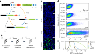
Human OPRM1 and murine Oprm1 promoter driven viral constructs for genetic access to μ-opioidergic cell types

Viral strategies for targeting spinal neuronal subtypes in adult wild-type rodents

Viral manipulation of functionally distinct interneurons in mice, non-human primates and humans

Data availability.

RNA-seq data are deposited in the NCBI Gene Expression Omnibus database with accession no. GSE224285 . Source data are provided with this paper.

Poulin, J.-F., Tasic, B., Hjerling-Leffler, J., Trimarchi, J. M. & Awatramani, R. Disentangling neural cell diversity using single-cell transcriptomics. Nat. Neurosci. 19 , 1131–1141 (2016).

Article   PubMed   Google Scholar  

Daigle, T. L. et al. A suite of transgenic driver and reporter mouse lines with enhanced brain-cell-type targeting and functionality. Cell 174 , 465–480.e22 (2018).

Article   CAS   PubMed   PubMed Central   Google Scholar  

Plummer, N. W. et al. Expanding the power of recombinase-based labeling to uncover cellular diversity. Development 142 , 4385–4393 (2015).

CAS   PubMed   PubMed Central   Google Scholar  

Fenno, L. E. et al. Targeting cells with single vectors using multiple-feature Boolean logic. Nat. Methods 11 , 763–772 (2014).

Fenno, L. E. et al. Comprehensive dual- and triple-feature intersectional single-vector delivery of diverse functional payloads to cells of behaving mammals. Neuron 107 , 836–853.e11 (2020).

Ren, J. et al. Single-cell transcriptomes and whole-brain projections of serotonin neurons in the mouse dorsal and median raphe nuclei. eLife 8 , e49424 (2019).

Pouchelon, G. et al. A versatile viral toolkit for functional discovery in the nervous system. Cell Rep. Methods 2 , 100225 (2022).

Chen, H.-S. et al. An intein-split transactivator for intersectional neural imaging and optogenetic manipulation. Nat. Commun. 13 , 3605 (2022).

Sabatini, P. V. et al. tTARGIT AAVs mediate the sensitive and flexible manipulation of intersectional neuronal populations in mice. eLife 10 , e66835 (2021).

Jeong, M. et al. Viral vector-mediated transgene delivery with novel recombinase systems for targeting neuronal populations defined by multiple features. Neuron 112 , 56–72.e4 (2024).

Article   CAS   PubMed   Google Scholar  

Han, H. J. et al. Strain background influences neurotoxicity and behavioral abnormalities in mice expressing the tetracycline transactivator. J. Neurosci. 32 , 10574–10586 (2012).

Zhu, P. et al. Silencing and un-silencing of tetracycline-controlled genes in neurons. PLoS ONE 2 , e533 (2007).

Article   PubMed   PubMed Central   Google Scholar  

Scott, W. G., Horan, L. H. & Martick, M. The hammerhead ribozyme: structure, catalysis, and gene regulation. Prog. Mol. Biol. Transl. Sci. 120 , 1–23 (2013).

Zhong, G. et al. A reversible RNA on-switch that controls gene expression of AAV-delivered therapeutics in vivo. Nat. Biotechnol. 38 , 169–175 (2020).

Strobel, B. et al. A small-molecule-responsive riboswitch enables conditional induction of viral vector-mediated gene expression in mice. ACS Synth. Biol. 9 , 1292–1305 (2020).

Poe, G. R. et al. Locus coeruleus: a new look at the blue spot. Nat. Rev. Neurosci. 21 , 644–659 (2020).

Knoll, A. T. & Carlezon, W. A. Jr. Dynorphin, stress, and depression. Brain Res. 1314 , 56–73 (2010).

Schnütgen, F. et al. A directional strategy for monitoring Cre-mediated recombination at the cellular level in the mouse. Nat. Biotechnol. 21 , 562–565 (2003).

Choi, J.-H. et al. Optimization of AAV expression cassettes to improve packaging capacity and transgene expression in neurons. Mol. Brain 7 , 17 (2014).

Fischer, K. B., Collins, H. K. & Callaway, E. M. Sources of off-target expression from recombinase-dependent AAV vectors and mitigation with cross-over insensitive ATG-out vectors. Proc. Natl Acad. Sci. USA 116 , 27001–27010 (2019).

Ringrose, L. et al. Comparative kinetic analysis of FLP and cre recombinases: mathematical models for DNA binding and recombination. J. Mol. Biol. 284 , 363–384 (1998).

Skofitsch, G. & Jacobowitz, D. M. Immunohistochemical mapping of galanin-like neurons in the rat central nervous system. Peptides 6 , 509–546 (1985).

Luskin, A. T. et al. A diverse network of pericoerulear neurons control arousal states. Preprint at bioRxiv https://doi.org/10.1101/2022.06.30.498327 (2022).

Tillage, R. P. et al. Co-released norepinephrine and galanin act on different timescales to promote stress-induced anxiety-like behavior. Neuropsychopharmacology 46 , 1535–1543 (2021).

Caramia, M. et al. Neuronal diversity of neuropeptide signaling, including galanin, in the mouse locus coeruleus. Proc. Natl Acad. Sci. USA 120 , e2222095120 (2023).

Borodovitsyna, O., Duffy, B. C., Pickering, A. E. & Chandler, D. J. Anatomically and functionally distinct locus coeruleus efferents mediate opposing effects on anxiety-like behavior. Neurobiol. Stress 13 , 100284 (2020).

Hirschberg, S., Li, Y., Randall, A., Kremer, E. J. & Pickering, A. E. Functional dichotomy in spinal- vs prefrontal-projecting locus coeruleus modules splits descending noradrenergic analgesia from ascending aversion and anxiety in rats. eLife 6 , e29808 (2017).

Uematsu, A. et al. Modular organization of the brainstem noradrenaline system coordinates opposing learning states. Nat. Neurosci. 20 , 1602–1611 (2017).

McCall, J. G. et al. Locus coeruleus to basolateral amygdala noradrenergic projections promote anxiety-like behavior. eLife 6 , e18247 (2017).

Pfeiffer, A., Brantl, V., Herz, A. & Emrich, H. M. Psychotomimesis mediated by kappa opiate receptors. Science 233 , 774–776 (1986).

Bilkei-Gorzo, A. et al. Dynorphins regulate fear memory: from mice to men. J. Neurosci. 32 , 9335–9343 (2012).

Wittmann, W. et al. Prodynorphin-derived peptides are critical modulators of anxiety and regulate neurochemistry and corticosterone. Neuropsychopharmacology 34 , 775–785 (2009).

Chandler, D. J., Gao, W.-J. & Waterhouse, B. D. Heterogeneous organization of the locus coeruleus projections to prefrontal and motor cortices. Proc. Natl Acad. Sci. USA 111 , 6816–6821 (2014).

Lein, E. S. et al. Genome-wide atlas of gene expression in the adult mouse brain. Nature 445 , 168–176 (2007).

Schwarz, L. A. et al. Viral-genetic tracing of the input–output organization of a central noradrenaline circuit. Nature 524 , 88–92 (2015).

Kebschull, J. M. et al. High-throughput mapping of single-neuron projections by sequencing of barcoded RNA. Neuron 91 , 975–987 (2016).

Reardon, T. R. et al. Rabies virus CVS-N2c(ΔG) strain enhances retrograde synaptic transfer and neuronal viability. Neuron 89 , 711–724 (2016).

Hang, A., Wang, Y.-J., He, L. & Liu, J.-G. The role of the dynorphin/κ opioid receptor system in anxiety. Acta Pharmacol. Sin. 36 , 783–790 (2015).

McCall, J. G. et al. CRH engagement of the locus coeruleus noradrenergic system mediates stress-induced anxiety. Neuron 87 , 605–620 (2015).

Zerbi, V. et al. Rapid reconfiguration of the functional connectome after chemogenetic locus coeruleus activation. Neuron 103 , 702–718.e5 (2019).

Sciolino, N. R. et al. Recombinase-dependent mouse lines for chemogenetic activation of genetically defined cell types. Cell Rep. 15 , 2563–2573 (2016).

Angenent-Mari, N. M., Garruss, A. S., Soenksen, L. R., Church, G. & Collins, J. J. A deep learning approach to programmable RNA switches. Nat. Commun. 11 , 5057 (2020).

Jang, S., Jang, S., Yang, J., Seo, S. W. & Jung, G. Y. RNA-based dynamic genetic controllers: development strategies and applications. Curr. Opin. Biotechnol. 53 , 1–11 (2018).

Peng, H., Latifi, B., Müller, S., Lupták, A. & Chen, I. A. Self-cleaving ribozymes: substrate specificity and synthetic biology applications. RSC Chem. Biol. 2 , 1370–1383 (2021).

Stage, T. K., Hertel, K. J. & Uhlenbeck, O. C. Inhibition of the hammerhead ribozyme by neomycin. RNA 1 , 95–101 (1995).

Wurmthaler, L. A., Sack, M., Gense, K., Hartig, J. S. & Gamerdinger, M. A tetracycline-dependent ribozyme switch allows conditional induction of gene expression in Caenorhabditis elegans . Nat. Commun. 10 , 491 (2019).

Zhong, G., Wang, H., Bailey, C. C., Gao, G. & Farzan, M. Rational design of aptazyme riboswitches for efficient control of gene expression in mammalian cells. eLife 5 , e18858 (2016).

DeNardo, L. & Luo, L. Genetic strategies to access activated neurons. Curr. Opin. Neurobiol. 45 , 121–129 (2017).

Vaaga, C. E., Borisovska, M. & Westbrook, G. L. Dual-transmitter neurons: functional implications of co-release and co-transmission. Curr. Opin. Neurobiol. 29 , 25–32 (2014).

Mulvey, B. et al. Molecular and functional sex differences of noradrenergic neurons in the mouse locus coeruleus. Cell Rep. 23 , 2225–2235 (2018).

Download references

Acknowledgements

We thank H. Sanders and K. Lowe for technical support, the St. Jude Vector Core Lab for generating ConVERGD AAVs, G. Neale and S. Olsen in the St. Jude Hartwell Center for Biotechnology for guidance with sequencing and members of the L.A.S. laboratory for helpful feedback. We also thank H. Zeng, A. Cetin, S. Yao, T. Zhou and M. T. Mortrud of the Allen Institute for sharing the N2c ΔG -H2B-eGFP virus for trans-synaptic tracing experiments and G. Zhong of Scripps Research, Florida for providing the initial sequence information for the T3H48 ribozyme. This work was supported by a NARSAD Young Investigator Grant from the Brain & Behavior Research Foundation (to L.A.S.), the NIH (grant no. 1DP2NS115764 to L.A.S.), institutional funds from St. Jude Children’s Research Hospital (to B.G.P., B.X., J.W.G. and L.A.S.) and funding from the St. Jude Graduate School of Biomedical Sciences (to A.C.H.). Single-cell sequencing was performed at the Hartwell Center at St. Jude, which is supported in part by the National Cancer Institute of the NIH under award no. P30 CA021765.

Author information

Authors and affiliations.

Department of Developmental Neurobiology, St. Jude Children’s Research Hospital, Memphis, TN, USA

Alex C. Hughes, Brittany G. Pittman, Jesse W. Gammons, Charis M. Webb, Hunter G. Nolen, Phillip Chapman, Jay B. Bikoff & Lindsay A. Schwarz

Human Cell Types, Allen Institute for Brain Science, Seattle, WA, USA

Alex C. Hughes

Center for Applied Bioinformatics, St. Jude Children’s Research Hospital, Memphis, TN, USA

You can also search for this author in PubMed   Google Scholar

Contributions

A.C.H. and L.A.S. conceived the project. A.C.H. designed ConVERGD, generated and tested viral constructs in vitro and in vivo and performed rabies tracing and behavioral studies. B.G.P. assisted with the cloning of viral constructs and in vitro testing. B.X. performed sequencing analysis. J.W.G. piloted manual sequencing methods and collected cells for sequencing. C.M.W. assisted with in vitro testing. H.G.N. assisted with behavioral testing. P.C. and J.B.B. provided the protocol and starter virus for generating N2c-rabies. L.A.S. generated viruses, performed in situ hybridization experiments, in vitro assessment of leak expression and in vivo testing and rabies-tracing experiments, and supervised the project. A.C.H. and L.A.S. wrote and edited the paper with feedback from the other authors.

Corresponding author

Correspondence to Lindsay A. Schwarz .

Ethics declarations

Competing interests.

The authors declare no competing interests.

Peer review

Peer review information.

Nature Neuroscience thanks Ryoji Amamoto, Els Henckaerts, Bernardo Sabatini and the other, anonymous, reviewer(s) for their contribution to the peer review of this work.

Additional information

Publisher’s note Springer Nature remains neutral with regard to jurisdictional claims in published maps and institutional affiliations.

Extended data

Extended data fig. 1 comparison of convergd-based constructs with varying promoter and posttranscriptional elements..

a , FACS quantification of N2a cells co-transfected with an EYFP- or eGFP-expressing plasmid alone (Control, grey bars) or with recombinase plasmids expressing Cre (yellow bars), Flp (blue bars), or Cre and Flp (pDIRE, green bars). ConVERGD was tested in pAAV backbones containing different promoters and 3′ posttranscriptional regulatory elements. b , FACS quantification as in a but represented as percent of live, single cells that were counted positive for fluorescence. Bars represent the mean of all experiments. Error bars are SEM. CV - ConVERGD. Data points represent independent transfections with the following constructs: 56 (FLEx(FRT)eGFP alone or +pDIRE), 6 (CV-eGFP-W3SL +Flp, +pDIRE; CV-eGFP-WPRE, +Flp, +pDire; Ef1a-CV-eGFP-WPRE, +pDIRE) 5 (INTRSECT-EYFP, +Cre, +Flp, +pDIRE; CV-eGFP-W3SL, +Cre; CV-eGFP-WPRE+Cre; nEF-CV-eGFP-WPRE, +pDIRE) 4 (CV-EYFP, +Flp; CAG-CV-eGFP-W3SL, +Cre, +Flp, +pDIRE; CAG-CV-eGFP-WPRE; Ef1a-CV-eGFP-W3SL, +Cre, +Flp, +pDIRE; Ef1a-CV-eGFP-WPRE+Cre, +Flp; nEF-CV-eGFP-W3SL, +Cre, +Flp, +pDIRE; nEF-CV-eGFP-WPRE+Cre, +Flp) 3 (CV-EYFP+Cre, +pDIRE; CAG-CV-eGFP-WPRE+Cre, +Flp, +pDIRE).

Extended Data Fig. 2 Assessment of leaky expression from ConVERGD and INTRSECT constructs.

a , Schematics for ConVERGD and INTRSECT constructs where no recombination has occurred, or upon Cre, Flp, or Cre and Flp-mediated recombination. Expected band sizes via PCR with specified primers are listed below. b , PCR of pAAV-hSyn-ConVERGD-eGFP-W3SL and pAAV-hSyn-INTRSECT-eYFP plasmids using the primer pairs described in a . c , Schematics for ConVERGD vectors where no recombination has occurred, or upon Cre, Flp, or Cre and Flp-mediated recombination. Schematics for vectors undergoing partial Flp-mediated recombination are also included. Expected band sizes via PCR with specified primers are listed below. d , Amplified PCR product from N2a cells transfected with hSyn-ConVERGD-eGFP-W3SL alone or with Cre, Flp, or Cre and Flp (pDIRE) expressing plasmids. mRNA extracted from these samples underwent a reverse transcriptase (RT) reaction to generate cDNA, or a no reverse transcriptase (no RT) reaction as a control. Each gel displays PCR products from template arising from the RT and no RT reactions. The gels are representative of results obtained across four independent sets of transfections. CV - ConVERGD; INTR – INTRSECT.

Source data

Extended data fig. 3 different recombination sites did not improve convergd performance..

a , FACS quantification of N2a cells co-transfected with ConVERGD-eGFP construct variants containing different recombinase recognition sites alone (Control, grey bars) or with recombinase plasmids expressing Cre (yellow bars), Flp (blue bars), or Cre and Flp (pDIRE, green bars). Data represented as the fold change of median fluorescence intensity (MFI) of transfection condition compared to the average control MFI for each construct. b , The same FACS quantification as in a but represented as percent of live, single cells that were counted positive for eGFP fluorescence. Data points represent individual transfection experiments. In a and b , results represent data from 7 (FRT5/FRT;loxP), 3 (FRT5/FRT;lox43/44), 6 (FRT5/FRT(min);loxP), 6 (FRT5/FRT(min);lox43/44) separate transfection experiments. Bars represent the mean of all experiments. Error bars are SEM.

Extended Data Fig. 4 Assessment of ConVERGD expression as percent of live N2a cells.

a , FACS quantification of N2a cells co-transfected with ConVERGD-ConFoff-eGFP (left) or ConVERGD-CoffFon-eGFP (right) either alone or with recombinase-expressing plasmid. b , FACS quantification of N2a cells co-transfected with ConVERGD-ConFonvCon-eGFP either alone or with recombinase-expressing plasmid. c , FACS quantification of N2a cells co-transfected with ConVERGD-ConFonvConNon-eGFP either alone or with recombinase-expressing plasmid. Data points in all panels represent the percent of live cells that contain eGFP from individual transfections. Data points represent independent transfections with the following constructs: 3 (CV-ConFoff-eGFP control; CV-ConFonvConNon-eGFP +Flp/Nigri, +vCre/Nigri, +vCre/Flp/Nigri, +Cre/Flp/vCre/Nigri), 4 (CV-ConFoff-eGFP +Cre, +Flp, +pDire; all conditions for ConFonvCon; CV-ConFonvConNon-eGFP +Cre/Flp/Nigri), 5 (CV-CoffFon-eGFP all conditions; CV-ConFonvConNon-eGFP +Cre/vCre, +Cre/Nigri, +Cre/Flp/vCre), 6 (CV-ConFonvConNon-eGFP, +Cre, +Flp, +vCre, +Cre/vCre/Nigri), 7 (CV-ConFonvConNon-eGFP +Nigri, +Flp/vCre), and 9 CV-ConFonvConNon-eGFP +Cre/Flp. Bars represent the mean of all experiments. Error bars are SEM.

Extended Data Fig. 5 ConVERGD-based constructs are easily amenable and allow specific expression of diverse transgenes.

a , ConVERGD-based toolkit for modulating neuronal activity. b , ConVERGD-based toolkit for trans-synaptic rabies tracing. c , ConVERGD-based construct for in vivo calcium imaging (GCaMP8m; GC8m). d , ConVERGD-based construct for a dual-expressing transgene that labels pre-synaptic sites and axons (synaptophysin-GreenLantern and GAP43-mScarlet). All images show transfected N2a cells counterstained with DAPI (blue) and are representative of results observed across at least two separate transfections. FR - FusionRed; mChr - mCherry; GL - GreenLantern; mSc - mScarlet. Scale bar in a is 100μm and applies to all images.

Extended Data Fig. 6 ConVERGD shows specific, intersectional expression in the hippocampus of Calb1 Cre ; Slc17a7 Flp mice.

a , Representative images of labeled cells in the hippocampus upon injection of Cre-dependent eGFP AAV in Calb1 Cre mice (left) or Flp-dependent mCherry AAV in Slc17a7 Flp mice (right). b , Representative images of AAV-hSyn-ConVERGD-eGFP or AAV-hSyn-INTRSECT-Con/Fon-EYFP injected into the hippocampus of Calb1 Cre , Slc17a7 Flp , and Calb1 Cre ; Slc17a7 Flp mice. Tissue sections in the top two rows reflect endogenous fluorescence while tissue sections in the bottom two rows were immunostained with GFP antibody. c , Representative images of AAV-hSyn-ConVERGD-ConFonvCon-eGFP injected into the hippocampus of Calb1 Cre ; Slc17a7 Flp mice in the absence (left) or presence (right) of vCre-expressing AAV. Tissue sections were immunostained with GFP antibody. d , Representative images of AAV-hSyn-ConVERGD-ConFoff-eGFP injected into the hippocampus of Calb1 Cre (left) or Calb1 Cre ; Slc17a7 Flp (right) mice. Tissue sections were immunostained with GFP antibody. e , Representative images of AAV-hSyn-ConVERGD-CoffFon-eGFP injected into the hippocampus of Slc17a7 Flp (left) or Calb1 Cre ; Slc17a7 Flp (right) mice. Tissue sections were immunostained with GFP antibody. Images in a , c, d , and e are representative of results across 2 mice for each genotype; images in b are representative of results across 3 mice for each genotype. Scale bars are 100μm. WT - wild-type; Calb1 - calbindin 1; Slc17a7 - solute carrier family 17 member 7; INTR - INTRSECT; CV - ConVERGD.

Extended Data Fig. 7 Top 100 most frequently detected genes in LC neurons using a Smart-seq2-based sequencing platform.

a , Heatmap of scaled (by cell) transcript abundance (transcripts per million, TPM) for the top 100 genes most frequently detected in 201 LC neurons by single-cell transcriptomic sequencing.

Extended Data Fig. 8 Increased single-recombinase induced expression observed with INTRSECT.

a , Representative images showing the LC (TH, white) of mice injected with AAV-hSyn-INTRSECT-Con/Fon-EYFP. All genotypes showed some level of YFP (green) expression. b , Quantification of INTRSECT-EYFP labeled cells in and around (~200μm radius) the LC across different genotypes. Points represent cell counts across 6 50μm LC brain sections. Bars represent the mean of the data. Error bars are SEM. All sections were immunostained against GFP. Images in a are representative of results observed across 4 ( Pdyn Cre ), 4 ( Dbh Flp ), and 5 ( Pdyn Cre ;Dbh Flp ) animals. Scale bars are 100μm. TH - tyrosine hydroxylase; LC - locus coeruleus; Pdyn - prodynorphin; Dbh - dopamine-β-hydroxylase.

Supplementary information

Supplementary information.

Supplementary Fig. 1.

Reporting Summary

Supplementary table 1.

Genetic space needed for intersectional machinery.

Supplementary Table 2

Key resource table.

Supplementary Code 1

Customized code used to analyze EZM experiments.

Supplemenatry Code 2

Source data fig. 7.

Source data for rabies-tracing experiments.

Source Data Fig. 8

Source data for behavior experiments.

Source Data Extended Data Fig. 2

Source gels for Extended Data Fig. 2.

Rights and permissions

Springer Nature or its licensor (e.g. a society or other partner) holds exclusive rights to this article under a publishing agreement with the author(s) or other rightsholder(s); author self-archiving of the accepted manuscript version of this article is solely governed by the terms of such publishing agreement and applicable law.

Reprints and permissions

About this article

Cite this article.

Hughes, A.C., Pittman, B.G., Xu, B. et al. A single-vector intersectional AAV strategy for interrogating cellular diversity and brain function. Nat Neurosci (2024). https://doi.org/10.1038/s41593-024-01659-7

Download citation

Received : 27 January 2023

Accepted : 22 April 2024

Published : 27 May 2024

DOI : https://doi.org/10.1038/s41593-024-01659-7

Share this article

Anyone you share the following link with will be able to read this content:

Sorry, a shareable link is not currently available for this article.

Provided by the Springer Nature SharedIt content-sharing initiative

Quick links

• Explore articles by subject
• Guide to authors
• Editorial policies

Sign up for the Nature Briefing: Translational Research newsletter — top stories in biotechnology, drug discovery and pharma.