excel random assignment to groups

Randomly assign data to groups

Related functions .

To randomly assign rows of data to arbitrary groups, you can use the RANDBETWEEN function with the CHOOSE function . In the example shown, the formula in F5 is:

As the formula is copied down the column, it will return a random group ("A", "B", or "C") at each new row.

Note: this approach will create groups of different sizes. If you need to assign random groups with a fixed size, see  this formula .

Generic formula

Explanation .

In this example, the goal is to return a random group ("A", "B", or "C") at each new row. The simplest way to do this is to use the RANDBETWEEN function with the CHOOSE function. In the current version of Excel, it is also possible to generate all random groups in one step with the RANDARRAY function. Both approaches are explained below.

The CHOOSE function

The CHOOSE function returns a value from a list of values using an index number. The index number is provided as the first argument, and the values to be selected follow. For example, if we have a list of three colors ("red", "blue", and "green"), we can configure CHOOSE to return each color in turn with the following formulas:

Notice that CHOOSE uses the index number to select the "nth" value from the list of values. The values can be customized in any way you like and the only requirement is that the index number be valid for the number of values provided. Of course, in this example, we don't want to hardcode an index number into CHOOSE, we want a random index number. For this, we can use the RANDBETWEEN function.

The RANDBETWEEN function

The RANDBETWEEN function generates a random number between two integers, provided as the bottom and the top . For example, to generate a random number between 1 and 10, you can use RANDBETWEEN like this:

When Excel's calculation engine updates a worksheet, RANDBETWEEN will generate a random number between 1 and 10.

CHOOSE with RANDBETWEEN

The behavior of RANDBETWEEN will work perfectly for this problem. We have three possible groups ("A","B","C") so we need a random number between 1 and 3, which we can get like this:

The final step is to embed RANDBETWEEN into the CHOOSE function as the index number like this:

This is the formula that appears in cell F5 in the example shown. When the formula is copied down the column, RANDBETWEEN returns a random number between 1 and 3. This number is delivered directly to the CHOOSE function as the index number, and CHOOSE returns the corresponding color as a final result. You can use this approach whenever you need to assign random text values to each row in a data set. Just be sure to adjust the second argument in RANDBETWEEN, top , to match the number of values provided.

Stopping automatic recalculation

Be aware that RANDBETWEEN is a volatile function and will recalculate whenever there is any change to a workbook, or even when a workbook is opened. To force a recalculation, you can press the F9 key. Once you have a set of random assignments, you may want to stop the formula from returning new results. The classic way to do this is to use Paste Special:

• Select all cells that contain the CHOOSE and RANDBETWEEN formula.
• Copy to the clipboard with Control + C.
• Open the Paste Special window with the shortcut Control + Alt + V.
• Select "Values" and click OK:

After you press OK, all formulas will be replaced with static values.

Dynamic array formula

In the current version of Excel (Excel 2021 or later) you can use a single dynamic array formula to generate all random values at once. One option is to use the RANDARRAY function with CHOOSE like this:

The core idea of this formula is the same as the original formula above. However, instead of RANDBETWEEN, we use RANDARRAY, which can generate an array of random numbers in one step. To figure out how many random numbers to generate, we use the ROWS function on a range corresponding to the first column of the data. This saves us the step of telling RANDARRAY how many rows we need. In this case, ROWS returns 100, because there are 100 rows in the range B5:B104. Simplifying, we now have:

Next, RANDARRAY generates an array of 100 random numbers between 1 and 3. The result is returned to CHOOSE as the index_num argument, and CHOOSE uses the random numbers to return an array that contains 100 random groups. This array lands in cell F5 and spills into the range F5:F104.

INDEX alternative

It is also possible to use the INDEX function instead of CHOOSE in a formula like this:

Like CHOOSE, INDEX retrieves a value based on an index number. INDEX however accepts the values all at once in the first argument, called array . In the formula above, the values "A", "B", and "C" are provided as an array constant to INDEX as the array , and RANDBETWEEN is used as before to generate a random number between 1 and 3.  The RANDARRAY version of the formula with INDEX looks like this:

One advantage of INDEX is that the array constant can be replaced with a range on the worksheet. In other words, you can enter group names into a range and provide that range to INDEX. The CHOOSE function will not accept a range of values; it requires that values be provided separately.

Note: the formulas on this page will create completely random groups. One result is that the total number of rows assigned to each group will vary. If you need to assign random groups with a fixed size (i.e. randomly assign people to teams of 6), see the example on  this page .

Related formulas

• Randomly assign people to groups

• Random number between two numbers

• Random date between two dates

• Random text values

• Random value from list or table

• Random number from fixed set of options

Related functions

• RANDBETWEEN Function

The Excel RANDBETWEEN function returns a random integer between two given numbers. RANDBETWEEN recalculates each time a worksheet is opened or changed.

• CHOOSE Function

The Excel CHOOSE function returns a value from a list using a given position or index. For example, =CHOOSE(2,"red","blue","green") returns "blue", since blue is the 2nd value listed after the index number. The values provided to CHOOSE can include references.

• RANDARRAY Function

The Excel RANDARRAY function generates an array of random numbers between two values. The size or the array is specified by rows and columns arguments. The generated values can be either decimals or whole numbers.

• ROWS Function

The Excel ROWS function returns the count of rows in a given reference. For example, ROWS(A1:A3) returns 3, since the range A1:A3 contains 3 rows.

Related videos

• How to pick names out of a hat with Excel

• How to randomly assign people to teams

Hi - I'm Dave Bruns, and I run Exceljet with my wife, Lisa. Our goal is to help you work faster in Excel. We create short videos, and clear examples of formulas, functions, pivot tables, conditional formatting, and charts.

Related Information

Get training, quick, clean, and to the point training.

Learn Excel with high quality video training. Our videos are quick, clean, and to the point, so you can learn Excel in less time, and easily review key topics when needed. Each video comes with its own practice worksheet.

Help us improve Exceljet

Your email address is private and not shared.

How to Randomize a List in Excel Into Groups (5 Suitable Ways)

In this article, I will show you how to randomize a list in Excel into groups. While working on an Excel worksheet, you need to do a massive type of work. Sometimes you may need to rank any dataset randomly. In this article, I will show you how to randomize a list   in Excel properly. I hope this article will increase your Excel skills. However, follow the procedures step-by-step. I have added pictures for your better understanding.

How to Randomize a List in Excel Into Groups: 5 Suitable Ways

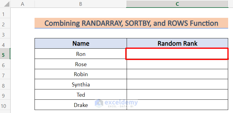
You can see the dataset I have used in this article in the following picture. The dataset has two columns called B and C . The dataset has the values called Student Id, and Name of students of a certain school. I will use this dataset to show how to randomize a list in Excel into groups. Follow the steps of every method one by one.

1. Randomize a List in Excel Into Groups Using RAND Function

In this method, you will know the randomization method of a list using the RAND function . The process is simple. Follow the procedures one by one. Hopefully, you will find interest in this method. I have made a slight change in the dataset. I am considering only the name column and added a new column called Random Rank here. However, follow the steps carefully.

• First, select the C5 cell and copy the following formula into it.

• After pressing Enter, you will find the following number.

• Then, Fill Handle the formula to copy down from C5 to C10 .

• Then, go to the Formula tab in your toolbar.
• After that, select the Calculation  option.
• Hence, select the manual option.

• Then, select the Home tab and go to the Editing  option.

• Then, select the Sort and Filter  option.

• Meanwhile, a pop-up window will appear. Select the Sort Largest to Smallest  option.

• Then, like the following window, select the Expand the Selection option and select the Sort  button.

• As a result, Excel will sort the Names like the following picture.

This is how the randomization of a list can happen.

Read More: List of Names for Practice in Excel

2. Implementing Excel RANDBETWEEN Function to Randomize a List

In this portion of this article, I will implement the RANDBETWEEN function to randomize a list in Excel. This is another short method. I hope this will increase your Excel skills. Follow the procedure step by step.

• First, select the C5  cell.

• Then, copy down the following formula in the selected cell.

• After pressing Enter , Excel will show the following result.

• Then, copy down the formula to the C10  cell.
• Hence, you will get random numbers like the picture given below.

• Moreover, to stop the automatic changing of the numbers, go to the Formulas tab and select the Calculation Options .
• Then, select the Manual  option.

• Then, go to the Home tab and select the Editing  option.

• After that, select the Sort & Filter  option.

• Hence, select the Sort Largest to Smallest  option.

• Meanwhile, the following window will appear. Select the Expand the selection option and then press the Sort  button.

• As a result, Excel will show the following sorted result.

This is how you can use the RANDBETWEEN function to randomize a list in Excel.

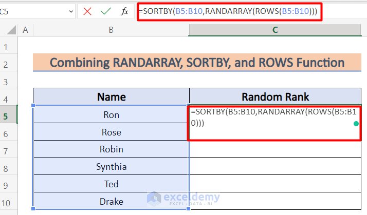
3. Combine RANDARRAY, SORTBY, and ROWS Functions

In this part of this article, I will Combine RANDARRAY, SORTBY, and ROWS Functions. This method is not as easy as the former two methods. Follow the method step by step given below.

• Then, copy the following formula in the selected cell.
• ROWS(B5:B10): Returns the row numbers of the array.
• RANDARRAY(ROWS(B5:B10): Returns an Array according to the ROWS
• SORTBY(B5:B10, RANDARRAY(ROWS(B5:B10))) : Returns the newly sorted names and spills the names throughout the whole column.

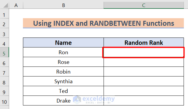
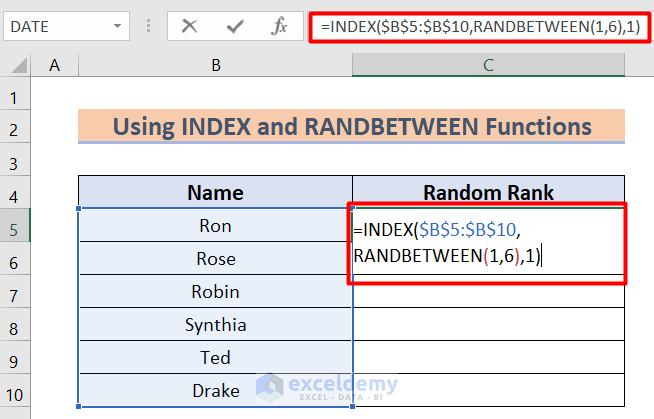
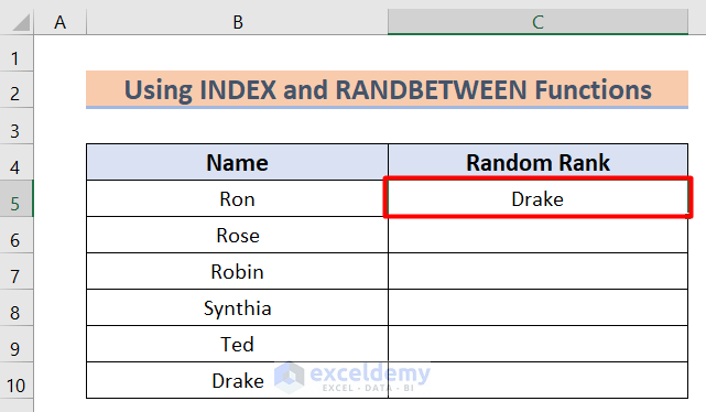
4. Using INDEX and RANDBETWEEN Functions

In this part of this article, I will use INDEX and RANDBETWEEN functions to randomize a list in Excel into groups. Follow the following steps to randomize the list.

• Select the C5 cell first.

• Then, write down the following formula in the selected cell.
• RANDBETWEEN(1,6): Returns a random number in a cell between 1 to 6.
• INDEX($B$5:$B$10, RANDBETWEEN(1,6),1): Returns randomly sorted names in a certain cell.

• After pressing Enter , the following result will be shown.

• After copying down the formula, Excel will show the following result.

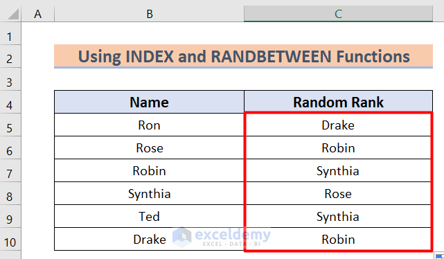
We can randomize a list in Excel using the INDEX and RANDBETWEEN Functions.

5. Applying CHOOSE and RANDBETWEEN Functions

In this method, I will apply CHOOSE and RANDBETWEEN functions to randomize a list in Excel into groups. Follow the following steps.

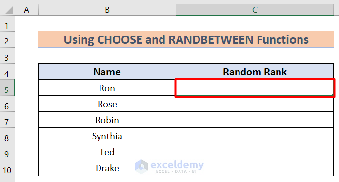
• Write down the following formula in the selected cell.
• CHOOSE(RANDBETWEEN(1,6),$B$5,$B$6,$B$7,$B$8,$B$9,$B$10): Returns the shuffled names in the C  column.

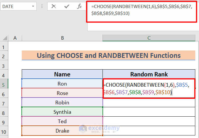
• Then, Copy down the formula from C5 to C10

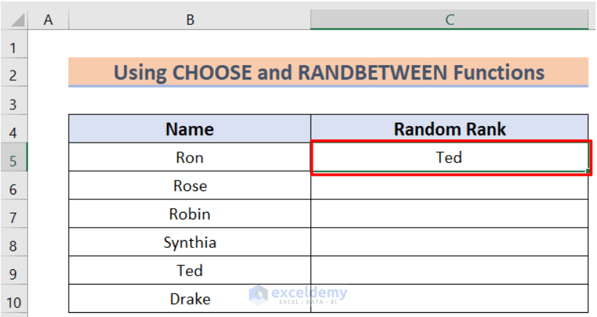
• Hence, the following result will be found.

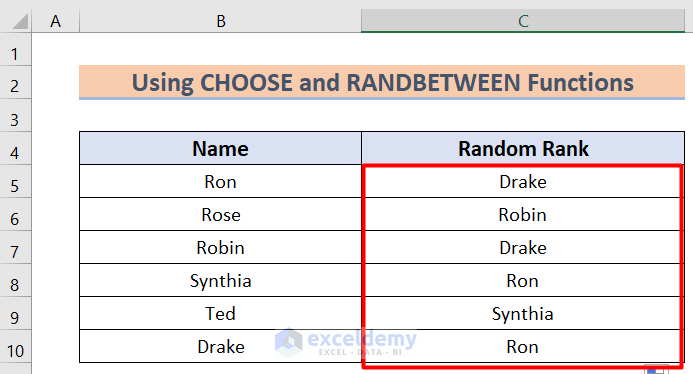
This is the procedure how to randomize a list in Excel into groups.

Read More: Excel Practice Exercises PDF with Answers

Things to Remember

• You should bear in mind that the SORTBY function can only be found in Excel 365.

Download Practice Workbook

In this article, I have tried to explain how to randomize a list in Excel into groups. I hope you have learned something new from this article. Now, extend your skill by following the steps of these methods. I hope you have enjoyed the whole tutorial. If you have any queries, feel free to ask me in the comment section. Don’t forget to give us your feedback.

<< Go Back to Randomize in Excel   |  Learn Excel

What is ExcelDemy?

Tags: Randomize in Excel

Souptik Roy, a BSc graduate in Naval Architecture and Marine Engineering from Bangladesh University of Engineering and Technology, dedicated 1.5 years to the ExcelDemy project. During this time, he authored 50+ articles and reviewed 20+ for ExcelDemy. Presently, he is a designer and content developer at YouHaveGotThisMath and Brainor, sister concerns of ExcelDemy. His educational content spans science, mathematics, and grammar. Roy's interests include developing creative ideas, visualizing concepts with tools like Adobe Illustrator, and problem-solving within Microsoft... Read Full Bio

Leave a reply Cancel reply

ExcelDemy is a place where you can learn Excel, and get solutions to your Excel & Excel VBA-related problems, Data Analysis with Excel, etc. We provide tips, how to guide, provide online training, and also provide Excel solutions to your business problems.

Contact  |  Privacy Policy  |  TOS

• User Reviews
• List of Services
• Service Pricing

• Create Basic Excel Pivot Tables
• Excel Formulas and Functions
• Excel Charts and SmartArt Graphics
• Advanced Excel Training
• Data Analysis Excel for Beginners

Advanced Excel Exercises with Solutions PDF

Statistics Made Easy

How to Create Random Groups in Excel (With Example)

Often you may want to create random groups in Excel.

For example, you might want to assign 12 basketball players to one of three random teams:

Fortunately this is easy to do and the following step-by-step example shows how to do so.

Step 1: Enter Original Data

First, let’s enter the names of 12 basketball players that we’d like to assign to random teams:

Step 2: Generate Random Values

Next, we will generate a random number between 0 and 1 for each player by typing the following formula into cell B2 :

We can then click and drag this formula down to each remaining cell in column B:

Each player now has a random value associated with them between 0 and 1.

Step 3: Generate Random Groups

Next, we will assign each player to a random group.

To do so, we will type the following formula into cell C2 :

We can then click and drag this formula down to each remaining cell in column C:

Column C now assigns each player to one of three random teams.

For example:

• Andy has been assigned to Team 2.
• Bob has been assigned to Team 2.
• Chad has been assigned to Team 1.

Note that the value after the division symbol in the formula specifies the number of players to include in each group.

For example, we could change this number from 4 to 6 to instead include 6 players on each team:

We can type this formula into cell C2 and then click and drag it down to each remaining cell in column C:

Notice that six players are now assigned to Team 1 and six players are assigned to Team 2.

Feel free to change the number after the division symbol in the formula to assign a different number of players to each team.

Additional Resources

The following tutorials explain how to perform other common operations in Excel:

How to Generate Random Number Between Range in Excel How to Randomly Select Cells Based on Criteria in Excel How to Select a Random Sample in Excel

Featured Posts

Hey there. My name is Zach Bobbitt. I have a Masters of Science degree in Applied Statistics and I’ve worked on machine learning algorithms for professional businesses in both healthcare and retail. I’m passionate about statistics, machine learning, and data visualization and I created Statology to be a resource for both students and teachers alike.  My goal with this site is to help you learn statistics through using simple terms, plenty of real-world examples, and helpful illustrations.

Leave a Reply Cancel reply

Your email address will not be published. Required fields are marked *

Join the Statology Community

Sign up to receive Statology's exclusive study resource: 100 practice problems with step-by-step solutions. Plus, get our latest insights, tutorials, and data analysis tips straight to your inbox!

By subscribing you accept Statology's Privacy Policy.

How to Generate Random Groups in Excel (Formula)

- Written by Puneet

• Random Groups with Random Size (CHOOSE + RANDBETWEEN)
• Random Groups with Same Size (RAND + ROUND + RANK)

In both methods, we need to write a formula. And in this tutorial, we will learn both ways and understand them in detail.

In this example, you have a list of students with their names, and now you need to assign them a random group from north, south, east, and west.

Generating Random Groups in Excel

To write this formula, you can use the below steps:

• First, in a cell, enter the CHOOSE function.
• And in the first argument of the CHOOSE, which is index_num enter the RANDBETWEEN function.
• Now, in the RANDBETWEEN, enter “1” as the bottom and “4” as the top. So you have four groups to get the result; that’s why you need to use 1 and 4 to create a range of random numbers.
• Next, in the second argument of CHOOSE, enter the name of all four groups by using double quotation marks (“North”,”South”,”East”,”West”).
• In the end, hit enter to get the result. And drag the formula up to the last name.

Note: RANBBETWEEN is a volatile function that updates itself when you change your worksheet.

How this Formula Works

To understand this formula, you need to split it into two parts: In the first part, we have RANDBETWEEN, which returns a random number between 1 to 4 (as we have four groups).

In the second part, we have CHOOSE function, which returns a value from the list you define using the index_number. When RANDBETWEEN returns a random number, CHOOSE returns the value from the list using that number.

When you have 3 in the index number, CHOOSE returns “East” in the result.

But there’s a Problem.

When you use this formula, there’s no same-size grouping. So you can see in the result that the groups assigned to the students are not of the same size.

This method is only proper when you don’t want to consider the group size; otherwise, you need to use the formula we will discuss next.

Generating Random Groups (Same Size)

To use this formula, you need to create a helper column with the RAND function to get the random number between 0 and 1, just like the following.

Note: RAND is also a volatile function that changes its value. And here, I’m going to convert the formula into values .

After that , enter a new column and the RANK function. Then, in the number argument, specify the random number from the B2; in the ref argument, use the entire range of random numbers.

It creates a unique ranking for all the 12 students you have on the list. Now , you need to divide this ranking by three, as you need to have three students in a single group.

Next , you need to use the ROUNDUP to round these rankings upwards.

After using ROUNDUP, you get an even size group where each group has the same number of students (12 students in the four groups with three students in each group). Then, again, use the CHOOSE to convert these number groups into group names.

Get the Excel File

Related formulas.

• Create a Horizontal Filter in Excel
• Create a Star Rating Template in Excel
• Get File Name in Excel
• Get Sheet Name in Excel
• Quickly Generate Random Letters in Excel
• Randomize a List (Random Sort) in Excel
• Count Characters in Excel (Cell and Range)
• Get File Path (Excel Formula)
• Get the Value from a Cell
• Compare Two Strings (Text)
• Get the Domain from the Email ID
• Extract Only Numbers from a Text (String)
• Extract Text After and Before a Character in Excel
• Back to the List of Excel Formulas

Schedule a Demo

How to randomly assign participants to groups in excel.

Too many steps?

Try sourcetable..

Randomly assigning participants to groups is a critical step in ensuring the validity of experimental research. Excel, with its built-in functions, allows for a variety of methods to perform this task.

However, Excel's procedures can be intricate and time-consuming. This guide will offer step-by-step instructions to simplify the process.

Additionally, we'll explore how Sourcetable provides a more streamlined and user-friendly approach for random assignment compared to Excel.

Randomly Assign Participants to Groups in Excel

Using randbetween and choose functions.

Utilize the RANDBETWEEN function to generate random numbers within a specific range, which can be used to assign participants to groups. Combine RANDBETWEEN with the CHOOSE function to allocate individuals to pre-defined groups.

Employing RAND Function for Randomization

Implement the RAND function to create a random number between 0 and 1 in a helper column. This function is essential for assigning a unique set of random values to participants in one step.

Using RAND and RANK Functions Together

Deploy the RAND function alongside RANK and ROUNDUP functions to distribute participants into groups. The ROUNDUP function is valuable for rounding numbers up to the nearest integer, facilitating group assignment.

Alternative Methods with CEILING Function

For an alternative to ROUNDUP, consider the CEILING function to assign random values more flexibly. This approach provides additional control over the assignment process.

Recalculation of Random Functions

Note that RANDBETWEEN and RAND functions recalculate every time the worksheet is opened or edited. Ensure that you finalize group assignments to prevent changes.

Common Use Cases

Excel vs. sourcetable: streamlined data integration and ai assistance.

Excel, a longstanding leader in spreadsheet software, is renowned for its comprehensive toolset that caters to various data manipulation needs. However, Sourcetable specializes in aggregating data from multiple sources into a single interface, simplifying data management.

Sourcetable's AI copilot differentiates it from Excel by offering users an innovative chat interface. This feature assists in generating formulas and templates, enhancing productivity and reducing the learning curve associated with complex spreadsheet functions.

While Excel requires manual setup for data integration, Sourcetable automates the process, enabling real-time data queries across platforms. This serves businesses that rely on up-to-date information from diverse data ecosystems.

The AI-enhanced capabilities of Sourcetable provide a user-friendly alternative to Excel's traditional formula creation. Users can leverage AI to streamline workflows and improve data analysis efficiency.

No guides needed. Ask Sourcetable AI

Recommended How To Guides

• How to... Randomly Select Rows In Excel
• How to... Use Randarray In Excel
• How to... Do A Frequency Distribution In Excel
• How to... Make A Seating Chart In Excel
• How to... Calculate Sample Proportion In Excel
• How to... Make A Population Pyramid In Excel

Start working with Live Data

Analyze data, automate reports and create live dashboards for all your business applications, without code. get unlimited access free for 14 days..

• Kutools for Excel
• Kutools for Outlook
• Kutools for Word
• Setup Made Simple
• End User License Agreement
• Get 4 Software Bundle
• 60-Day Refund
• Tips & Tricks for Excel (3000+)
• Tips & Tricks for Outlook (1200+)
• Tips & Tricks for Word (300+)
• Excel Functions (498)
• Excel Formulas (350)
• Excel Charts
• Outlook Tutorials
• About Us Our Team

Feature Tutorials

• Search Search more
• Retrieve License Lost License?
• Report a Bug Bug Report
• Forum Post in Forum

Quickly generate random groups for list of data in Excel

Sometimes, you may want to randomly assign data to groups as screenshot 1 shown, or generate groups for a list of names as below screenshot 2 shown, but how can handle these jobs quickly? Actually, in Excel, you can use formulas to solve them easily.

Randomly assign data to groups

Generate random groups in a specified data size, download sample file.

If you want to randomly assign data to a specified number of groups, each group is allowed with different numbers of data, you can use the CHOOSE and RANDBETWEEN functions.

Select a blank cell next to the list you want to assign to random groups, copy or type this formula

=CHOOSE(RANDBETWEEN(1,3),"Group A","Group B","Group C ")

In the formula, (1, 3) indicates to group data into 3 groups, Group A, Group B and Group C are the texts will be displayed in formula cells which used to distinguish different groups.

Then the list of data has been randomly assigned to groups, and each group may have different numbers of data.

The calculated results will not be fixed, they will be recalculated if there is any change to the workbook.

If you want to generate random groups for a list of data, and each group has a specified data size, you can use the ROUNDUP and RANK functions.

1. Firstly, you need a helper column to list some random data next to your data. Supposing in cell E2, type this formula

Then drag fill handle down to fill this formula to cells you use.

2. In the next column, supposing in cell F2, copy or type this formula

=ROUNDUP(RANK(E2,$E$2:$E$13)/4,0)

E2:E13 is the range that contains formula =RAND(), 4 is the number of data that you want each group contains.

Click to download sample file

Other Popular Articles

Remove first or last n characters from a cell or string in Excel

Extract part of text string from cell in Excel?

Two Easy Ways to convert or import Word document contents to Excel worksheet

Calculate the absolute difference between two values/times in Excel

More articles

Excel Productivity Tools

The best office productivity tools, kutools for excel solves most of your problems, and increases your productivity by 80%.

• Super Formula Bar (easily edit multiple lines of text and formula); Reading Layout (easily read and edit large numbers of cells); Paste to Filtered Range ...
• Merge Cells/Rows/Columns and Keeping Data; Split Cells Content; Combine Duplicate Rows and Sum/Average ... Prevent Duplicate Cells; Compare Ranges ...
• Select Duplicate or Unique Rows; Select Blank Rows (all cells are empty); Super Find and Fuzzy Find in Many Workbooks; Random Select...
• Exact Copy Multiple Cells without changing formula reference; Auto Create References to Multiple Sheets; Insert Bullets , Check Boxes and more...
• Favorite and Quickly Insert Formulas , Ranges, Charts and Pictures; Encrypt Cells with password; Create Mailing List and send emails...
• Extract Text , Add Text, Remove by Position, Remove Space ; Create and Print Paging Subtotals; Convert Between Cells Content and Comments ...
• Super Filter (save and apply filter schemes to other sheets); Advanced Sort by month/week/day, frequency and more; Special Filter by bold, italic...
• Combine Workbooks and WorkSheets ; Merge Tables based on key columns; Split Data into Multiple Sheets ; Batch Convert xls, xlsx and PDF ...
• Pivot Table Grouping by week number, day of week and more... Show Unlocked, Locked Cells by different colors; Highlight Cells That Have Formula/Name ...

Office Tab - brings tabbed interface to Office, and make your work much easier

• Enable tabbed editing and reading in Word, Excel, PowerPoint , Publisher, Access, Visio and Project.
• Open and create multiple documents in new tabs of the same window, rather than in new windows.
• Increases your productivity by 50%, and reduces hundreds of mouse clicks for you every day!

• Ablebits blog
• Random data

RANDARRAY function - quick way to generate random numbers in Excel

The tutorial shows how to generate random numbers, randomly sort a list, get random selection and randomly assign data to groups. All with a new dynamic array function - RANDARRAY.

As you probably know, Microsoft Excel already has a couple of randomizing functions - RAND and RANDBETWEEN . What is the sense in introducing another one? In a nutshell, because it's far more powerful and can replace both older functions. Apart from setting up your own maximum and minimum values, it lets you specify how many rows and columns to fill and whether to produce random decimals or integers. Used together with other functions, RANDARRAY can even shuffle data and pick a random sample.

Excel RANDARRAY function

• Basic RANDARRAY formula

Generate random numbers between two numbers

Generate random date between two dates.

• Create random workdays in Excel
• Generate random numbers without duplicates
• Random sort in Excel
• Get a random sample
• Select random rows
• Random assignment in Excel
• Randomly assign data to groups

Excel RANDARRAY function not working

The RANDARRAY function in Excel returns an array of random numbers between any two numbers that you specify.

It is one of six new dynamic array functions introduced in Microsoft Excel 365. The result is a dynamic array that spills into the specified number of rows and columns automatically.

The function has the following syntax. Please notice that all the arguments are optional:

Rows (optional) - defines how many rows to fill. If omitted, defaults to 1 row.

Columns (optional) - defines how many columns to fill. If omitted, defaults to 1 column.

Min (optional) - the smallest random number to produce. If not specified, the default 0 value is used.

Max (optional) - the largest random number to create. If not specified, the default 1 value is used.

Whole_number (optional) - determines what kind of values to return:

• TRUE - whole numbers
• FALSE or omitted (default) - decimal numbers

RANDARRAY function - things to remember

To efficiently generate random numbers in your Excel worksheets, there are 6 important points to take notice of:

• The RANDARRAY function is only available in Excel for Microsoft 365 and Excel 2021. In Excel 2019, Excel 2016 and earlier versions the RANDARRAY function is not available.
• If the array returned by RANDARRAY is the final result (output in a cell and not passed to another function), Excel automatically creates a dynamic spill range and populates it with the random numbers. So, be sure you have enough empty cells down and/or to the right of the cell where you enter the formula, otherwise a #SPILL error will occur.
• If none of the arguments is specified, a RANDARRAY() formula returns a single decimal number between 0 and 1.
• If the rows or/and columns arguments are represented by decimal numbers, they will be truncated to the whole integer before the decimal point (e.g. 5.9 will be treated as 5).
• If the min or max argument is not defined, RANDARRAY defaults to 0 and 1, respectively.
• Like other random functions, Excel RANDARRAY is volatile , meaning it generates a new list of random values every time the worksheet is calculated. To prevent this from happening, you can replace formulas with values by using Excel's Paste Special > Values feature.

Basic Excel RANDARRAY formula

And now, let me show you a random Excel formula in its simplest form.

Supposing you want to fill a range consisting of 5 rows and 3 columns with any random numbers. To have it done, set up the first two arguments this way:

• Rows is 5 since we want the results in 5 rows.
• Columns is 3 as we want the results in 3 columns.

All of the other arguments we leave to their default values and get the following formula:

=RANDARRAY(5, 3)

How to randomize in Excel - RANDARRAY formula examples

Below you will find a few advanced formulas that cover typical randomizing scenarios in Excel.

To create a list of random numbers within a specific range, supply the minimum value in the 3 rd argument and the maximum number in the 4 th argument. Depending on whether you need integers or decimals, set the 5 th argument to TRUE or FALSE, respectively.

As an example, let's populate a range of 6 rows and 4 columns with random integers from 1 to 100. For this, we set up the following arguments of the RANDARRAY function:

• Rows is 6 since we want the results in 6 rows.
• Columns is 4 as we want the results in 4 columns.
• Min is 1, which is the minimum value we wish to have.
• Max is 100, which is the maximum value to be generated.
• Whole_number is TRUE because we need integers.

Putting the arguments together, we get this formula:

=RANDARRAY(6, 4, 1, 100, TRUE)

Looking for a random date generator in Excel? The RANDARRAY function is an easy solution! All you have to do is input the earlier date (date 1) and later date (date 2) in predefined cells, and then reference those cells in your formula:

For this example, we have created a list of random dates between the dates in D1 and D2 with this formula:

Of course, nothing prevents you from supplying the min and max dates directly in the formula if you wish to. Just be sure you enter them in the format that Excel can understand:

=RANDARRAY(10, 1, "1/1/2020", "12/31/2020", TRUE)

To prevent mistakes, you can use the DATE function for entering dates:

=RANDARRAY(10, 1, DATE(2020,1,1), DATE(2020,12,31), TRUE)

Generate random workdays in Excel

To produce random working days, embed the RANDARRAY function in the first argument of WORKDAY like this:

RANDARRAY will create an array of random start dates, to which the WORKDAY function will add 1 workday and ensure that all the returned dates are working days.

With date 1 in D1 and date 2 in D2, here's the formula to produce a list of 10 weekdays:

How to generate random numbers without duplicates

Though modern Excel offers 6 new dynamic array functions, unfortunately, there is still no inbuilt function to return random numbers without duplicates.

To build your own unique random number generator in Excel, you will need to chain several functions together like shown below.

Random integers :

Random decimals :

• N is how many values you wish to generate.
• Min is the lowest value.
• Max is the highest value.

For example, to produce 10 random whole numbers with no duplicates, use this formula:

To create a list of 10 unique random decimal numbers , change TRUE to FALSE in the last argument of the RANDARRAY function or simply omit this argument:

Tips and notes:

• The detailed explanation of the formula can be found in How to generate random numbers in Excel without duplicates .
• In Excel 2019 and earlier, the RANDARRAY function is not available. Instead, please check out this solution .

How to randomly sort in Excel

To shuffle data in Excel, use RANDARRAY for the "sort by" array ( by_array argument) of the SORTBY function . The ROWS function will count the number of rows in your data set, indicating how many random numbers to generate:

With this approach, you can randomly sort a list in Excel, whether it contains numbers, dates or text entries:

Also, you can also shuffle rows without mixing your data:

How to get a random selection in Excel

To extract a random sample from a list, here's a generic formula to use:

Where n is the number of random entries you wish to extract.

For example, to randomly select 3 names from the list in A2:A10, use this formula:

=INDEX(A2:A10, RANDARRAY(3, 1, 1, ROWS(A2:A10), TRUE))

Or input the desired sample size in some cell, say C2, and reference that cell:

How this formula works:

At the core of this formula is the RANDARRAY function that creates a random array of integers, with the value in C2 defining how many values to generate. The minimal number is hardcoded (1) and the maximum number corresponds to the number of rows in your data set, which is returned by the ROWS function.

The array of random integers goes directly to the row_num argument of the INDEX function, specifying the positions of the items to return. For the sample in the screenshot above, it is:

=INDEX(A2:A10, {8;7;4})

How to select random rows in Excel

If your data set contains more than one column, then specify which columns to include in the sample. For this, supply an array constant for the last argument ( column_num ) of the INDEX function, like this:

=INDEX(A2:B10, RANDARRAY(D2, 1, 1, ROWS(A2:A10), TRUE), {1,2})

Where A2:B10 is the source data and D2 is the sample size.

How to randomly assign numbers and text in Excel

To do random assignment in Excel, use RANDBETWEEN together with the CHOOSE function in this way:

• Data is a range of your source data to which you want to assign random values.
• N is the total number of values to assign.
• Value1 , value2 , value3 , etc. are the values to be assigned randomly.

For example, to assign numbers from 1 to 3 to participants in A2:A13, use this formula:

For convenience, you can enter the values to assign in separate cells, say from D2 to D4, and reference those cells in your formula (individually, not as a range):

=CHOOSE(RANDARRAY(ROWS(A2:A13), 1, 1, 3, TRUE), D2, D3, D4)

How this formula works

At the heart of this solution is again the RANDARRAY function that produces an array of random integers based on the min and max numbers that you specify (from 1 to 3 in our case). The ROWS function tells RANDARRAY how many random numbers to generate. This array goes to the index_num argument of the CHOOSE function . For example:

=CHOOSE({1;2;1;2;3;2;3;3;1;3;1;2}, D2, D3, D4)

How to randomly assign data to groups

When your task is to randomly assign participants to groups, the above formula may not be suitable because it does not control how many times a given group is chosen. For example, 5 persons could be assigned to group A while only 2 persons to group C. To do random assignment evenly , so that each group has the same number of participants, you need a different solution.

First, you generate a list of random numbers by using this formula:

=RANDARRAY(ROWS(A2:A13))

And then, you assign groups (or anything else) by using this generic formula:

Where n is the group size, i.e. the number of times each value should be assigned.

For example, to randomly assign people to the groups listed in E2:E5, so that each group has 3 participants, use this formula:

=INDEX($E$2:$E$5, ROUNDUP(RANK(B2,$B$2:$B$13)/3,0))

Please notice that it's a regular formula (not a dynamic array formula!), so you need to lock the ranges with absolute references like in the above formula.

Please remember that the RANDARRAY function is volatile. To prevent generating new random values every time you change something in the worksheet, replace formulas with their values by using the Paste Special feature.

The RANDARRAY formula in the helper column is very simple and hardly requires explanation, so let us focus on the formula in column C.

The RANK function ranks the value in B2 against the array of random numbers in B2:B13. The result is a number between 1 and the total number of participants (12 in our case).

The rank is divided by the group size, (3 in our example), and the ROUNDUP function rounds it up to the nearest integer. The result of this operation is a number between 1 and the total number of groups (4 in this example).

When your RANDARRAY formula returns an error, these are the most obvious reasons to check:

#SPILL error

#value error.

A #VALUE! error may occur in these circumstances:

• If a max value is less than a min value.
• If any of the arguments is non-numeric.

#NAME error

In most cases, a #NAME! error indicates one of the following:

• The function's name is misspelled.
• The function is not available in your Excel version.

#CALC! error

That's how to build a random number generator in Excel with the new RANDARRAY function. I thank you for reading and hope to see you on our blog next week!

Practice workbook for download

You may also be interested in.

• How to select random sample in Excel
• How to sort randomly in Excel
• How to generate random numbers in Excel with no repeats
• Flash Fill in Excel with examples

Table of contents

S. No Date Time Shift Day Subject Session Group

S.No Date Time Shift Day Subject Session Group

Formula in excel

Hi! We have a special tutorial that can help to solve your problem: How to convert rows to columns in Excel (transpose data) .

how to random array with the total of each row is 100?

I think you can try to use the custom functions and macros described in this article to create a random array with a specific sum in a row: How to find all combinations of numbers that equal given sum in Excel .

I always get a #name error

Hi, This error most often appears if you specified the function name incorrectly.

Post a comment

404 Not found

• CELL REFERENCE

Post your problem and you'll get expert help in seconds

• All articles

How to Set Up a Random Team Generator in Excel

Excel allows us to create a random team generator using the RAND, RANK and CEILING functions. This step by step tutorial will assist all levels of Excel users to learn how to set up a random team generator in Excel.

Syntax of the RAND Formula

The generic formula for the RAND function is:

The function returns a random decimal number between 0 and 1 and has no parameters.

Syntax of the RANK Formula

The generic formula for the RANK function is:

=RANK(number, ref, [order])

The parameters of the RANK function are:

• number – a number which we want to rank
• ref – a list of numbers for ranking
• [order] – 1 for ascending or 0 for descending order. This parameter is optional, if it’s omitted, the default order is descending.

Syntax of the CEILING Formula

The generic formula for the CEILING function is:

=CEILING(number, significance)

• number – a number which we want to round up to the nearest significance
• significance – a significance for rounding a number up.

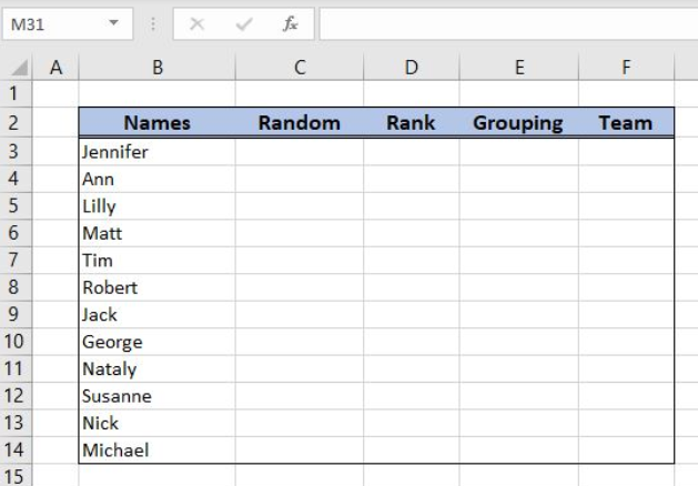
Setting up Our Data for the Formula

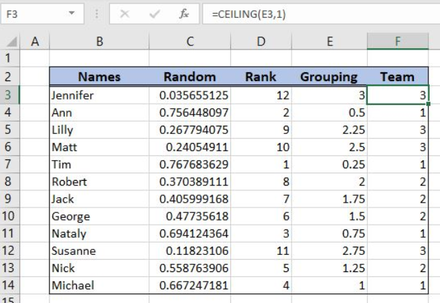
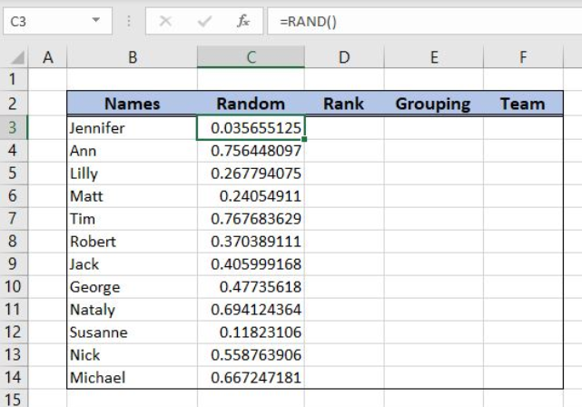
Let’s look at the data that we will use in the example. To group names into teams, we will need to have several helper columns. In column B (“Names”), we have names of team members. In column C (“Random”), we will have a random number 0-1 for every name. In column D (“Rank”), we will get a rank for every random number. In column E (“Grouping”), we’ll divide the rank with 3, as we have 3 teams. Finally, in column F (“Team”), we’ll get the team (1, 2 or 3) for each name

Set up a Random Team Generator

First, we need to get a random number in column C for each name.

The formula for RAND in C3 looks like:

To apply the formula, we need to follow these steps:

• Select cell C3 and click on it
• Insert the formula: =RAND()
• Press enter
• Drag the formula down to the other cells in the column by clicking and dragging the little “+” icon at the bottom-right of the cell.

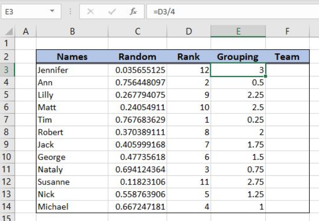
When we get a random number for each name we can rank them in column D.

The formula for RANK in C3 looks like:

=RANK(C3, $C$3:$C$14)

The number parameter is the cell C3. The ref parameter is the range $C$3:$C$14. We must fix the range, as it’s not changing when the formula is copied down the cells.

• Select cell D3 and click on it
• Insert the formula: =RANK(C3,$C$3:$C$14)

Now we have the rank for every random number in column D and can divide them by 3.

The formula in E3 looks like:

• Select cell E3 and click on it
• Insert the formula: =RANK/D3

Finally, we can use the CEILING formula, to assign team 1, 2 or 3 to each name.

The formula for CEILING in F3 looks like:

=CEILING(E3, 1)

The parameter number is the cell E3, while the significance is 1.

• Select cell F3 and click on it
• Insert the formula: =CEILING(E3,1)

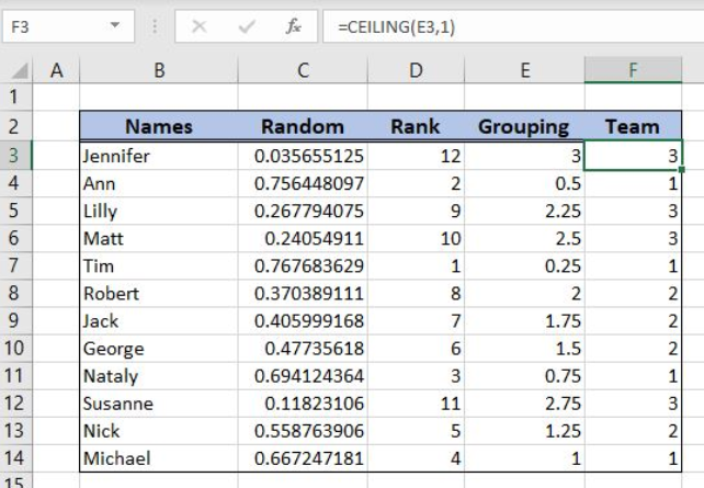
As you can see in Figure 6, in “Team” column we have assigned a team for each name from column B.

Most of the time, the problem you will need to solve will be more complex than a simple application of a formula or function. If you want to save hours of research and frustration, try our live Excelchat service! Our Excel Experts are available 24/7 to answer any Excel question you may have. We guarantee a connection within 30 seconds and a customized solution within 20 minutes.

Leave a Comment

Subscribe to Excelchat.co

Get updates on helpful Excel topics

Privacy & Cookies: This site uses cookies. By continuing to use this website, you agree to their use.

Save time by asking instead! Most questions solved and answered in 10 minutes.

Random Group Generator Template [FREE Download]

If you’re a teacher or a trainer, creating groups of students/participants is a common task. For example, you may want to create groups to conduct a quiz or a team building activity.

And in most of the cases, you need these groups to be random.

Today, I am sharing a random group generator template that will make it super easy for you to create a group of students/participants.

All you need is the list of students or participants and specify how many groups you want to create.

Random Group Generator Template

Here is a demo of how this random group generator (or random team generator) template works:

The list of students/participants is in A2:A17. If you have a longer list, simply add the names in it.

Cell E2 has the number of groups that you want to create. Based on the number you enter, you would get the groups and the names in each group in columns G to P. As of now, I have created it this template for a maximum of 10 groups.

Once you have entered the number of groups you want in cell E2, click on the ‘Create Teams’ button to randomly generate the groups of names.

Download the Random Group Generator Template

How this Excel Template Works

There are a couple of cool Excel features and a few helper columns that make this random group generator template in Excel.

Here is how it is made:

• In cell G2, this formula will pick up the rank from C2 and return the name at that position in the list.
• In cell G3, it will pick the rank from C6 (which is 1 + 1*4, where 4 is the number of groups to be formed).
• In cell G4, it will pick the rank from C10 (which is 1 + 2*4, where 4 is the number of groups to be formed).

Since RANDBETWEEN function is volatile , it will automatically refresh every time you make a change in the worksheet. This may be undesirable as it will change the grouping every time.

To avoid this:

• Go to File Options.
• In the Excel Options dialog box, select formulas in the pane on the left.

Now the worksheet would not refresh until you force a refresh by hitting the F9 key.

But to make it look better, there is an orange button that does the refresh when you click it. There is a one-line VBA code at play here that gets executed whenever you click the button.

Here is how to insert this button:

• Close the VB Editor.

• Format the button the way you want.

Now when you click on the button, the worksheet would recalculate and you would get a new grouping based on the number of groups you have specified.

Other Excel Templates You May Like:

• Employee Leave/Vacation Tracker Template .
• Employee Timesheet Calculator .
• Excel To Do Lists Templates .
• A collection of FREE Excel Templates .

You may also like the following Excel tutorials:

• How to Generate Unique Random Numbers in Excel .
• How to Run a Macro in Excel .
• How to Create an Excel Dashboard .
• How to Rank within Groups in Excel
• How to Shuffle a List of Items/Names in Excel? 2 Easy Formulas!

FREE EXCEL BOOK

Get 51 Excel Tips Ebook to skyrocket your productivity and get work done faster

25 thoughts on “Random Group Generator Template [FREE Download]”

I need to add columns like, Last name, email address, Gender, City, and two more columns. Can you please guide me on how to work on the VBA so that I can use your template?

Is there any way to increase the max number of groups? I really need 15 groups! Please help… would be so great to use in my classroom.

I am sorry but the random team generator isn’t working correctly. It will pull duplicates about every 8th run. Conditional format for dups and you will see. Can it be fixed? I have trying but to no avail. Please advise. M

Thank you …i almost got here myself but couldn’t figure put how to add the names to the teams…awesome!

Thanks for the template! Is there a way to specify that I would want to have my samples distributed randomly across three groups (A,B,C) but have e.g. 80% of them in group-A, 10% in group-B and 10% in group-C?

Doesnt work, can anyone help. Why does the formual reference cell F if there is nothing in it?

You can help me to create a specific random match, is for a sport team, 6 teams with 3 members i need matching with rival teams and similar weight for the member or very close weight , please i pay you

This is a great tool. However I tried modifying it. But could’nt.

I just need 1 Team where I need to mention the no of members in cell E2 and it creates a team with Random Names. I am confident its a piece of cake for you.

Absolutely perfect but I need the absent function to work. I would love to this to randomly select 3 or 4 ball groups of golfers whilst we are on the tee. However we are never sure who is going to turn up hence the need to mark golfers absent from the master list and randomise the selection of the players who are there. Can anyone help???

Sorry this does not work very well. I have 40 teams and they have to be paired this goes no where needed for this program to work.

Hey there, Loved this! i ended up making a few alterations of my own, namely, put the generating function into VBA so that it stopped updating all the time, I added some arrows to increase/decrease the number of groups with a single click and also made a ‘secret’ tab where you could specify two people you didn’t want in the same group. I’d be happy to share it if you’re interested.

Hi Steve, Please do share how you worked on “secret” tab.

Is there a way to set group 1 to have 10 members, and the others to have like 7 ?

Cool trick, but i have one scenario. let’s say i have names(2 or more) that cannot be teamed together,is there any way to solve it?

Hi Sumit! This is amazing for my classroom thanks so much! Is there any way to increase the max number of groups? I really need 12 groups!

Dear Sumit,

I really enjoy using your random group generator for my classes (I created a tab for each class. It’s swift and easy to use.

Sometimes, however someone in a class is absent (visit to the dentist, etc.). If so, I have to alter the table, to remove the absent student.

It would be nice if there could be a column next to the student names where I could mark the absent student(s) (for example with a zero) , so he/she won’t be displayed in the generated groups.

Unfortunately I don’t have the programming skills to make that happen.

Someone else perhaps?

Greetings, Willem (Netherlands)

Thanks Willem.. Glad you liked it.

Here is a link to a new template that will allow you to mark a student as absent: https://www.dropbox.com/s/ys1mmwmbdy7eeb5/Random-Team-Generator-Template%20Absent.xlsm?dl=0

Hello… there is something wrong with the absent function in the worksheet…Even if I indicate that the student is absent, his name will still show in the generated teams list… Also, is there anyway to group 40 people into 2 groups… it seems that the template doesn’t support such a function… thanks and keep up the good work! 🙂

Hello, I was searching for an excel template to create random 4 man teams when I happened upon your template. I downloaded it and tested what I am trying to accomplish, but was having trouble when I found the above link. It gets me a step closer to what I am wanting to do, however, I am trying to accomplish the opposite. I have a list of 71, but I only want to include those I identify as opposed to excluding those that are identified. And I want the teams to be in multiples of 4, but I think if I identify the total number of teams, the template will provide me with teams of 3 or 4. So, I am wondering if a template is available that would provide the capability to include vs exclude? Thanks in advance for your help. Andy.

Thanks to both of you, Sumit and Rudra! Sumit, I enjoy your formulabased random generator. I have my ovn VBA-generator that I will continue using,but I learned a lot from your reallønn Nice formulas.

Rudra! I’ve never notised the easy way of changing calculation mode. I still miss a warning light when ExCeL is in manual mode. Forgetting to return to aut. Mode has caised me lot f extra work.

From the Custom Quick Access Toolbaar, add “Manual” to the Quick Access Toolbaar and it will show when in Manual mode.

Thanks Hennie, I’ve already adferd it to QAT.

Cool trick Sumit. Thanks for sharing. However there is a short cut to change calculation from ribbon itself. Just go to formula ribbon and click on Calculation Option.

Thanks for sharing Rudra.. That’s definitely the faster way to do this.

Leave a Comment Cancel reply

BEST EXCEL TUTORIALS

Best Excel Shortcuts

Conditional Formatting

Excel Skills

Creating a Pivot Table

Excel Tables

INDEX- MATCH Combo

Creating a Drop Down List

Recording a Macro

© TrumpExcel.com – Free Online Excel Training

Privacy Policy  | Sitemap

Twitter | Facebook | YouTube | Pinterest | Linkedin

FREE EXCEL E-BOOK

• [email protected]
• +14372198199

How to Make Random Groups in Excel?

Random Groups in Excel can be a powerful tool for various applications, from statistical sampling to team assignments in a workplace setting. Creating these groups manually can be time-consuming and prone to bias, making Excel’s randomization functions a valuable asset. Whether you’re a researcher conducting a randomized control trial, a teacher assigning project groups, or a manager distributing tasks among teams, this guide will navigate you through the steps to efficiently generate random groups in Excel. By harnessing the power of Excel’s randomization features, you can ensure fairness and objectivity in your group assignments, while saving time and enhancing the overall efficiency of your organizational processes.

This Content Covers:

• Use of RANDBETWEEN Function
• Use of CHOOSE Function
• Use of combining RANDBETWEEN and CHOOSE Functions
• Explanation of formula
• CEILING Function
• Explanation of CEILING function
• Explanation with example

1. Make Random Groups in Excel

In certain situations, it may be desirable to generate groups for a list of names or randomly allocate data to groups. You can quickly create random groups for a set of data in Microsoft Excel by using a formula.

The RANDBETWEEN and CHOOSE Functions can be used to randomly allocate items (data, people, etc.) to groups.

Procedure of using RANDBETWEEN Function

Step 1: Next to the list you want to divide into random groups, choose a blank cell, then enter the RANDBETWEEN function, outlined in Red below.

After applying the function or formula, the result looks like below.

Step 2: After that, to fill all the cells, pull the “Fill Handle” further. The result is outlined in Red below.

• Use of CHOOSE Function:

Procedure of using CHOOSE Function:

Step 1: Next to the list you want to divide into random groups, choose a blank cell, then enter the CHOOSE function, outlined in Red below.

• Use of combination of RANDBETWEEN and CHOOSE Functions

Combining the two allows us to assign teams to groups by randomly “choosing” one item from a list.

Procedure of combining RANDBETWEEN and CHOOSE Functions:

Step 1: Next to the list you want to divide into random groups, choose a blank cell, then enter the function or formula, outlined in Red below.

2.Randomly assign people in the groups in Excel

Sometimes we have to pick groups at random. Although it could appear like a difficult undertaking, Excel makes it incredibly simple to complete by using formula.

Here, we may make use of a formula produced by combining the Excel RANK and ROUNDUP tools. Additionally, we employ a helper column where the RAND function is utilized to produce values at random.

We use the formula to assign individuals into groups at random.

=ROUNDUP(RANK(A1,randoms)/size,0)

For each element, the aforementioned formula returns a group number.

“size” and “randoms” are called range.

The Excel RAND function creates the helper column “Random”.

• Explanation of formula:

The Excel RANK function is a built-in feature that provides the position of a given number in an array or huge collection of numbers. In Excel, this function falls under the category of built-in statistical function.

Another built-in function in Excel is the ROUNDUP function, which returns a value that has been rounded to a predetermined number of digits. This function deviates from zero. It can be used effectively as an Excel worksheet function and is categorized as a Trig or Math function.

Procedure of assigning people in the groups randomly in Excel

Step 1: Let’s use a case where we have to assign teams to random groups. We apply the formula shown in D2 to build groups.

3. Alternative solution

The CEILING function, another built-in Excel function, can be used as an alternate method of assigning random values.

• CEILING Function:

We can use CEILING function or formula to assign individuals into groups at random.

=CEILING(RANK(C5,random)/size,1)

• Explanation of CEILING function:

In place of the ROUNDUP function, you can use this function. The ceiling function rounds up, but it does so to a specific multiple rather than to a specific number of decimal places.

• Explanation with example:

Procedure of assigning people in the groups randomly in Excel using CEILING function:

Here, “random” is the name of the range [C2:C13] and “size” is the named range[G5].

You may be interested:

• Financial Dashboards
• Sales Dashboards
• HR Dashboards
• Data Visualization Charts

Leave a Comment Cancel Reply

Your email address will not be published. Required fields are marked *

Save my name, email, and website in this browser for the next time I comment.

• Count Characters
• Count if method in Excel
• Print in Excel
• Bar Chart with Bubble in Top
• Dual Axis Chart
• Dumbbell DNA Chart
• Give Axis in Chart
• Half circle KPI chart
• Line Chart in Excel
• Mirror Bar Chart
• Progress Chart In Excel
• Side by Side Bar Chart
• Speedometer Chart
• Stacked Column Chart
• Timeline Chart
• ABS Function
• ACCRINT function in Excel
• ACOS Function in Excel
• Add Column in Excel
• Add Plus Sign Before Numbers
• Alphabetize by last name
• Amortization Schedule in Excel
• AREAS Function in Excel
• ASIN Function in Excel
• ATAN and ATAN2 Function
• AutoFit Column Width
• Automatic Formatting
• AVEDEV Function in Excel
• Bell Curve in Excel
• BETADIST Function in Excel
• BETAINV Function in Excel
• BIN2DEC Function in Excel
• Box and Whisker Plot in Excel
• Bullet Points in Excel
• Calculate Age in Excel
• Calculate Confidence Interval
• Calculate Correlation Coefficient
• Calculate Discounted Price
• Calculate Percentage Change
• Calculate Quarter from date
• Calculate Square Root
• Calculate the Area
• Calculate the week ending date
• Calculate Workdays in Excel
• Calculate Years of Service
• Calculated Field in Pivot Table
• Calculating BMI in Excel
• Calculating Simple Interest
• Capitalize First Letter in Excel
• Cell Reference in Excel
• Change Row Height
• Change the Negative Numbers to Zero
• Check Mark Symbol
• Check Not Equal To in Excel
• Check Text or Number
• Circular Reference
• Clean Data in Excel
• CLEAN Function in Excel
• Clear Formatting in Cell
• Clear Table Formatting
• CODE Function in Excel
• Color Scales in Excel
• COLUMN Function
• Combine Date and Time in Excel
• Combine Names in Excel
• Compare Columns in Excel
• Compare Text in Excel
• Compare Texts of Two Cells
• Compare Two Dates
• Compound Annual Growth Rate
• Compound Interest Formula
• CONCAT function in Excel
• CONCATENATE Excel
• Conditional Formatting in Excel
• Conditional Formatting to Pivot Table
• Confidence Interval in Excel
• Convert Date to Text
• Convert Date to Text in Excel
• Convert Excel to PDF
• Convert Formulas to Values
• Convert KG to LBS in Excel
• Convert Serial Number to Date
• Convert Text to Number
• Convert XML files to Excel
• Copy and Paste Multiple Cells
• Copy Conditional Formatting to Another Cell
• Copy Excel Formula
• Copy formula in Excel
• CORREL function in Excel
• COS Function in Excel
• COSH function in Excel
• Count Cells with Text
• Count Characters in Excel
• Count Colored Cells
• COUNT Function
• Count Unique Values
• COUNTBLANK Function
• COUNTIF – COUNTIFS Function
• COUPDAYBS Function
• Create a Custom List
• Create and Install Excel Add In
• Create and Use Scroll Bar
• Create and Use Workbooks
• Create budget in Excel
• CRITBINOM function in Excel
• Criteria Validity in Excel
• CUMPRINC Function in Excel
• Dashboard in Excel
• Data Entry Form
• Data Formatting in Excel
• Data Validation in Excel
• DATEDIF Function in Excel
• DATEVALUE Function
• DAVERAGE Function in Excel
• DAYS360 Function in Excel
• DEGREES function in excel
• Delete Blank Rows
• Delete Hidden Rows
• Delete Pivot Table
• Delete Rows Based on Cell Value
• Delta symbol in Excel
• Developer Tab in Excel
• DMIN function in Excel
• Drop-Down List in Excel
• DSUM Function in Excel
• DURATION function in Excel
• DVAR function in excel
• Dynamic Named Range
• Email from Excel Sheet
• Enable Macro
• EOMONTH Function in Excel
• Excel Camera Tool
• Excel File Not Open
• Excel IFERROR Function
• Excel Interview Question
• Excel MAX Function
• Excel RAND and RANDBETWEEN Function
• Excel RANK Function
• Excel REPLACE and SUBSTITUTE
• Excel SUMPRODUCT Function
• Excel Templates
• Excel VBA ASC Function
• Excel VBA TRIM Function
• Exponents in Excel
• Extract Dates in Excel
• Extract Numbers from Cell
• F-Test in Excel
• File Names list
• Fill Handle in Excel
• Fill Sequential Data
• Filter in Excel
• Find and Remove Outliers
• Find and Replace in Excel
• FIND and SEARCH Function
• Find Merged Cells
• Find Range in Excel
• Fix Excel Formula
• Fix Slow Excel Spreadsheets
• Flip Data in Excel
• Format Painter in Excel
• Formatting Shortcuts in Excel
• Freeze Rows and Columns
• Function Keys in Excel
• Future value of the annuity
• Generate Random Number
• Get Month name from date in Excel
• Greater Than or Equal to
• Gridlines in Excel
• Group in pivot table
• Heat Map in Excel
• Hide Formulas in Excel
• Hide Sheets in Excel
• Highlight Active Row Column
• Highlight Blank Cells and Fill Down Blank Cells
• HLOOKUP Function in Excel
• Hyperlink in Excel
• IF – AND Function
• IF – OR Function
• IF -AND-OR Function
• IFERROR with VLOOKUP to Replace #N/A Error
• Income tax bracket in excel
• Indent in Excel
• INDEX and MATCH Functions
• Index Match Formula in Excel
• INDIRECT – OFFSET Function
• Insert (Embed) PDF in Excel
• Insert and Delete Comments
• Insert Data and Timestamps
• Insert Degree Symbol in Excel
• Insert Line Break
• Integral or In-Built Themes
• Internal Rate of Return in Excel
• Intersect Operator
• Intersect Operator in Excel
• IRR in Excel
• ISNA Function
• Keyboard shortcuts
• Leading Zeros in Excel
• Linear Regression Analysis
• LINEST function in Excel
• lock and hide cells and protect worksheet
• Logical Functions in Excel
• Lookup and Reference Functions
• Make Scatter Plot
• Match Function in Excel
• Merge Cells in Excel
• Merge Two Columns
• Merge Two or More Tables
• MID Function in Excel
• MINIFS Function in Excel
• Mixed Reference
• MOD Function in Excel
• Month Name to Number
• Months to a date
• Mortgage Payment in Excel
• Move Row Column
• Multiple Columns in Excel
• Multiple option in a Drop Down
• Multiple Selections in Drop Down
• Multiplication in excel
• Multiply Column in Excel
• Named Range in Excel
• Negative Number to Positive
• New Excel Formulas
• NPER for Excel
• Number of Days Between Two Dates
• Offset Function in Excel
• Open and Use Visual Basic Editor
• Outline (group) Data
• Paste special in Excel
• Paste Special Shortcuts in Excel
• Picture Lookup
• Pivot Chart in Excel
• Chart from Pivot Table
• Filter in Pivot Table
• Number Formatting in Pivot Table
• Slicer in Pivot Table
• PMT function
• Print Title in Excel
• Print top rows
• PROPER Function
• Protect Excel File
• PV function in Excel
• Quadratic Equation
• Radio Button (Option Button)
• Radio Button Option
• Random Groups in Excel
• Record Macro in Excel
• Reduce Excel file size
• Reference Another Workbook
• Refresh Pivot Table
• Remove Dotted Lines
• Remove Duplicates
• Remove line breaks
• Remove Macro in Excel
• Remove Space in Excel
• Remove Time from Date
• Return Cell Address
• Rotate Text in Cells
• ROUND Function in Excel
• ROUNDUP and ROUNDDOWN
• Run Macro in Excel
• Scenario Manager in Excel
• Searchable Drop-Down List
• Select Multiple Cells
• Set Print Area in Excel
• Shade or Color Alternate Rows
• Show Formulas
• Shuffle Items in Excel
• Slicer in Excel
• Slicers in Pivot Table
• Slope in Excel
• Sort Data by Color in Excel
• Sort in Excel
• Sparklines in Excel
• Spell Check in Excel
• Standard Deviation in Excel
• Status Bar in Excel
• Stop numbers to dates
• Strikethrough Text in Excel
• Subtraction in Excel
• Sum Positive Numbers in Excel
• Superscript and Subscript
• T.TEST in Excel
• Text in Pivot Table
• Text to Column
• TODAY’s Date Function
• Top 10 Values in Excel
• Track Change
• Transpose in Excel
• Turn on AutoSave in Excel
• Two variable data table
• Unhide Columns
• Unhide Sheet in Excel
• Unmerge Cells in Excel
• Usage of 103 functions
• UserForm Excel
• VBA Message Box in Excel
• Weekdays in Excel
• Weighted Average Formula
• What-If Analysis in Excel
• Wrap Text in Excel
• XLOOKUP Function
• Zoom in and Zoom out

Contact Info

Find us on Social Media

Our Address

273 Pharmacy Avenue Toronto, ON M1L3E9

© 2023 All rights reserved | Biz Infograph

Excel Tutorial: How To Randomly Pair Names In Excel

Introduction.

Randomly pairing names in Excel can be a useful tool for organizing groups, creating pairs for projects or events, or conducting experiments . In this tutorial, we will walk through the step-by-step process of how to randomly pair names in Excel using a simple formula, making it easier for you to efficiently and fairly assign partners or groups.

Key Takeaways

• Randomly pairing names in Excel is a useful tool for organizing groups, creating pairs for projects or events, or conducting experiments.
• Properly formatting and ensuring uniqueness of names is crucial for the random pairing process.
• The RAND function can be used to generate random numbers for each name in Excel.
• Sorting the data based on the random numbers is essential for creating unique and fair pairings.
• Additional tips such as using the RANDBETWEEN function and creating a macro can enhance the random pairing process in Excel.

Understanding the Data

Before you can randomly pair names in Excel, it's important to ensure that the data is properly formatted and free of any duplicates.

Begin by checking that all the names are entered into a single column in your Excel spreadsheet. If the names are currently scattered across multiple columns, you can easily consolidate them into one by using the CONCATENATE function or simply copy and paste them into a single column.

It's crucial to eliminate any duplicate names from your list before proceeding with the random pairing. To achieve this, select the column containing the names, go to the 'Data' tab, and click on 'Remove Duplicates.' This will ensure that each name is unique and that there are no repetitions in your data set.

Using the RAND Function

When it comes to randomly pairing names in Excel, the RAND function is an essential tool. By using this function, you can generate random numbers that will allow you to pair up names in a fair and unbiased manner.

The RAND function in Excel is used to generate a random number between 0 and 1. This function is recalculated every time a worksheet is modified, which means the random numbers will change every time the worksheet is opened or modified. This makes it perfect for creating random pairings without any bias.

To start pairing names randomly, you will first need to create a list of names in your Excel worksheet. Once your list is ready, you can apply the RAND function to generate a random number for each name. This can be achieved by using the formula =RAND() in a separate column next to the list of names. By dragging the fill handle down, you can apply the formula to generate a random number for each name.

Sorting the Data

When it comes to randomly pairing names in Excel, sorting the data is an important step to ensure that the pairings are truly random and unique. Here's how you can go about it:

First, you'll need to generate a column of random numbers next to the list of names. You can do this by using the RAND() function in Excel. Simply enter =RAND() in the first cell next to the list of names, and then drag the fill handle down to generate random numbers for each name.

Once you have the list of names and their corresponding random numbers, you can use the SORT function to sort the list based on the random numbers. This will effectively randomize the order of the names, preparing them for pairing.

To ensure that the pairings are unique and not repeated, you can use conditional formatting to highlight any duplicate pairings. This will allow you to easily identify and rectify any repeated pairings, ensuring fairness and randomness in the process.

Finalizing the Pairings

After generating the random numbers and sorting the names accordingly, the next step is to finalize the pairings for your project or event. This involves creating a second column to pair the names based on the sorted random numbers and double-checking the pairings to ensure accuracy.

Once you have sorted the names based on the random numbers generated in the previous steps, you can create a second column to pair the names together. This can be done by simply listing the names in pairs next to the sorted list of names. For example, if the first two names in the sorted list are "John" and "Sarah", you would pair them together in the second column. Continue this process until all names are paired up.

B. Double-checking the pairings to ensure accuracy

Before finalizing the pairings, it's crucial to double-check the list to ensure accuracy. This can be done by reviewing the pairings and comparing them to the original list of names. Make sure that each name is paired with a different name and that no names are repeated within the pairings. This step is essential to avoid any errors in the pairings and ensure fairness in the random pairing process.

Additional Tips and Tricks

Once you've mastered the basics of randomly pairing names in Excel, you can take your skills to the next level with these additional tips and tricks.

If you want to generate random numbers within a specific range, you can use the RANDBETWEEN function. This function allows you to specify the minimum and maximum values for the range of random numbers that you want to generate. This can be useful if you have a predefined list of names and you want to pair them with a set of unique random numbers.

• 1. Open your Excel workbook and select the cell where you want the random number to appear.
• 2. Enter the formula =RANDBETWEEN(min,max) , replacing min with the minimum value of the range and max with the maximum value of the range.
• 3. Press Enter to generate a random number within the specified range.

If you find yourself frequently needing to randomly pair names in Excel, you can save time by creating a macro to automate the process. A macro is a series of commands and functions that can be recorded and then executed with a single click. By creating a macro for random pairing, you can quickly generate random pairs of names without having to manually input the formulas each time.

• 1. Go to the "Developer" tab and click on "Record Macro".
• 2. Name your macro and assign a shortcut key if desired.
• 3. Perform the actions of randomly pairing names in Excel while the macro is being recorded.
• 4. Click on "Stop Recording" once you have completed the pairing process.

Now, whenever you need to randomly pair names in Excel, you can simply run the macro to automate the entire process.

Recap: Randomly pairing names in Excel can be a useful tool for creating fair groups for activities or assignments, as well as for conducting random selections for surveys or research purposes. It can also help in maintaining confidentiality and fairness in certain situations.

Encouragement: As you practice pairing names in Excel, don't hesitate to explore additional functions and features for data manipulation. Excel offers a wide range of tools that can enhance your data management and analysis skills, making you more efficient and effective in your work.

Immediate Download

MAC & PC Compatible

Free Email Support

Related aticles

The Benefits of Excel Dashboards for Data Analysts

Unlock the Power of Real-Time Data Visualization with Excel Dashboards

Unlocking the Potential of Excel's Data Dashboard

Unleashing the Benefits of a Dashboard with Maximum Impact in Excel

Exploring Data Easily and Securely: Essential Features for Excel Dashboards

Unlock the Benefits of Real-Time Dashboard Updates in Excel

Unleashing the Power of Excel Dashboards

Understanding the Benefits and Challenges of Excel Dashboard Design and Development

Leverage Your Data with Excel Dashboards

Crafting the Perfect Dashboard for Excel

An Introduction to Excel Dashboards

How to Create an Effective Excel Dashboard

• Choosing a selection results in a full page refresh.