null hypothesis test regression

Statistics Made Easy

Understanding the Null Hypothesis for Linear Regression

Linear regression is a technique we can use to understand the relationship between one or more predictor variables and a response variable .

If we only have one predictor variable and one response variable, we can use simple linear regression , which uses the following formula to estimate the relationship between the variables:

ŷ = β 0 + β 1 x

ŷ: The estimated response value.
β 0 : The average value of y when x is zero.
β 1 : The average change in y associated with a one unit increase in x.
x: The value of the predictor variable.

Simple linear regression uses the following null and alternative hypotheses:

H 0 : β 1 = 0
H A : β 1 ≠ 0

The null hypothesis states that the coefficient β 1 is equal to zero. In other words, there is no statistically significant relationship between the predictor variable, x, and the response variable, y.

The alternative hypothesis states that β 1 is not equal to zero. In other words, there is a statistically significant relationship between x and y.

If we have multiple predictor variables and one response variable, we can use multiple linear regression , which uses the following formula to estimate the relationship between the variables:

ŷ = β 0 + β 1 x 1 + β 2 x 2 + … + β k x k

β 0 : The average value of y when all predictor variables are equal to zero.
β i : The average change in y associated with a one unit increase in x i .
x i : The value of the predictor variable x i .

Multiple linear regression uses the following null and alternative hypotheses:

H 0 : β 1 = β 2 = … = β k = 0
H A : β 1 = β 2 = … = β k ≠ 0

The null hypothesis states that all coefficients in the model are equal to zero. In other words, none of the predictor variables have a statistically significant relationship with the response variable, y.

The alternative hypothesis states that not every coefficient is simultaneously equal to zero.

The following examples show how to decide to reject or fail to reject the null hypothesis in both simple linear regression and multiple linear regression models.

Example 1: Simple Linear Regression

Suppose a professor would like to use the number of hours studied to predict the exam score that students will receive in his class. He collects data for 20 students and fits a simple linear regression model.

The following screenshot shows the output of the regression model:

Output of simple linear regression in Excel

The fitted simple linear regression model is:

Exam Score = 67.1617 + 5.2503*(hours studied)

To determine if there is a statistically significant relationship between hours studied and exam score, we need to analyze the overall F value of the model and the corresponding p-value:

Overall F-Value: 47.9952
P-value: 0.000

Since this p-value is less than .05, we can reject the null hypothesis. In other words, there is a statistically significant relationship between hours studied and exam score received.

Example 2: Multiple Linear Regression

Suppose a professor would like to use the number of hours studied and the number of prep exams taken to predict the exam score that students will receive in his class. He collects data for 20 students and fits a multiple linear regression model.

Multiple linear regression output in Excel

The fitted multiple linear regression model is:

Exam Score = 67.67 + 5.56*(hours studied) – 0.60*(prep exams taken)

To determine if there is a jointly statistically significant relationship between the two predictor variables and the response variable, we need to analyze the overall F value of the model and the corresponding p-value:

Overall F-Value: 23.46
P-value: 0.00

Since this p-value is less than .05, we can reject the null hypothesis. In other words, hours studied and prep exams taken have a jointly statistically significant relationship with exam score.

Note: Although the p-value for prep exams taken (p = 0.52) is not significant, prep exams combined with hours studied has a significant relationship with exam score.

Additional Resources

Understanding the F-Test of Overall Significance in Regression How to Read and Interpret a Regression Table How to Report Regression Results How to Perform Simple Linear Regression in Excel How to Perform Multiple Linear Regression in Excel

Featured Posts

7 Best YouTube Channels to Learn Statistics for Free

Hey there. My name is Zach Bobbitt. I have a Masters of Science degree in Applied Statistics and I’ve worked on machine learning algorithms for professional businesses in both healthcare and retail. I’m passionate about statistics, machine learning, and data visualization and I created Statology to be a resource for both students and teachers alike. My goal with this site is to help you learn statistics through using simple terms, plenty of real-world examples, and helpful illustrations.

2 Replies to “Understanding the Null Hypothesis for Linear Regression”

Thank you Zach, this helped me on homework!

Great articles, Zach.

I would like to cite your work in a research paper.

Could you provide me with your last name and initials.

Join the Statology Community

Sign up to receive Statology's exclusive study resource: 100 practice problems with step-by-step solutions. Plus, get our latest insights, tutorials, and data analysis tips straight to your inbox!

By subscribing you accept Statology's Privacy Policy.

Want to create or adapt books like this? Learn more about how Pressbooks supports open publishing practices.

13.6 Testing the Regression Coefficients

Learning objectives.

Conduct and interpret a hypothesis test on individual regression coefficients.

Previously, we learned that the population model for the multiple regression equation is

[latex]\begin{eqnarray*} y & = & \beta_0+\beta_1x_1+\beta_2x_2+\cdots+\beta_kx_k +\epsilon \end{eqnarray*}[/latex]

where [latex]x_1,x_2,\ldots,x_k[/latex] are the independent variables, [latex]\beta_0,\beta_1,\ldots,\beta_k[/latex] are the population parameters of the regression coefficients, and [latex]\epsilon[/latex] is the error variable. In multiple regression, we estimate each population regression coefficient [latex]\beta_i[/latex] with the sample regression coefficient [latex]b_i[/latex].

In the previous section, we learned how to conduct an overall model test to determine if the regression model is valid. If the outcome of the overall model test is that the model is valid, then at least one of the independent variables is related to the dependent variable—in other words, at least one of the regression coefficients [latex]\beta_i[/latex] is not zero. However, the overall model test does not tell us which independent variables are related to the dependent variable. To determine which independent variables are related to the dependent variable, we must test each of the regression coefficients.

Testing the Regression Coefficients

For an individual regression coefficient, we want to test if there is a relationship between the dependent variable [latex]y[/latex] and the independent variable [latex]x_i[/latex].

No Relationship . There is no relationship between the dependent variable [latex]y[/latex] and the independent variable [latex]x_i[/latex]. In this case, the regression coefficient [latex]\beta_i[/latex] is zero. This is the claim for the null hypothesis in an individual regression coefficient test: [latex]H_0: \beta_i=0[/latex].
Relationship. There is a relationship between the dependent variable [latex]y[/latex] and the independent variable [latex]x_i[/latex]. In this case, the regression coefficients [latex]\beta_i[/latex] is not zero. This is the claim for the alternative hypothesis in an individual regression coefficient test: [latex]H_a: \beta_i \neq 0[/latex]. We are not interested if the regression coefficient [latex]\beta_i[/latex] is positive or negative, only that it is not zero. We only need to find out if the regression coefficient is not zero to demonstrate that there is a relationship between the dependent variable and the independent variable. This makes the test on a regression coefficient a two-tailed test.

In order to conduct a hypothesis test on an individual regression coefficient [latex]\beta_i[/latex], we need to use the distribution of the sample regression coefficient [latex]b_i[/latex]:

The mean of the distribution of the sample regression coefficient is the population regression coefficient [latex]\beta_i[/latex].
The standard deviation of the distribution of the sample regression coefficient is [latex]\sigma_{b_i}[/latex]. Because we do not know the population standard deviation we must estimate [latex]\sigma_{b_i}[/latex] with the sample standard deviation [latex]s_{b_i}[/latex].
The distribution of the sample regression coefficient follows a normal distribution.

Steps to Conduct a Hypothesis Test on a Regression Coefficient

[latex]\begin{eqnarray*} H_0: & & \beta_i=0 \\ \\ \end{eqnarray*}[/latex]

[latex]\begin{eqnarray*} H_a: & & \beta_i \neq 0 \\ \\ \end{eqnarray*}[/latex]

Collect the sample information for the test and identify the significance level [latex]\alpha[/latex].

[latex]\begin{eqnarray*}t & = & \frac{b_i-\beta_i}{s_{b_i}} \\ \\ df & = & n-k-1 \\ \\ \end{eqnarray*}[/latex]

The results of the sample data are significant. There is sufficient evidence to conclude that the null hypothesis [latex]H_0[/latex] is an incorrect belief and that the alternative hypothesis [latex]H_a[/latex] is most likely correct.
The results of the sample data are not significant. There is not sufficient evidence to conclude that the alternative hypothesis [latex]H_a[/latex] may be correct.
Write down a concluding sentence specific to the context of the question.

The required [latex]t[/latex]-score and p -value for the test can be found on the regression summary table, which we learned how to generate in Excel in a previous section.

The human resources department at a large company wants to develop a model to predict an employee’s job satisfaction from the number of hours of unpaid work per week the employee does, the employee’s age, and the employee’s income. A sample of 25 employees at the company is taken and the data is recorded in the table below. The employee’s income is recorded in $1000s and the job satisfaction score is out of 10, with higher values indicating greater job satisfaction.

Previously, we found the multiple regression equation to predict the job satisfaction score from the other variables:

[latex]\begin{eqnarray*} \hat{y} & = & 4.7993-0.3818x_1+0.0046x_2+0.0233x_3 \\ \\ \hat{y} & = & \mbox{predicted job satisfaction score} \\ x_1 & = & \mbox{hours of unpaid work per week} \\ x_2 & = & \mbox{age} \\ x_3 & = & \mbox{income (\$1000s)}\end{eqnarray*}[/latex]

At the 5% significance level, test the relationship between the dependent variable “job satisfaction” and the independent variable “hours of unpaid work per week”.

Hypotheses:

[latex]\begin{eqnarray*} H_0: & & \beta_1=0 \\ H_a: & & \beta_1 \neq 0 \end{eqnarray*}[/latex]

The regression summary table generated by Excel is shown below:

The p -value for the test on the hours of unpaid work per week regression coefficient is in the bottom part of the table under the P-value column of the Hours of Unpaid Work per Week row . So the p -value=[latex]0.0082[/latex].

Conclusion:

Because p -value[latex]=0.0082 \lt 0.05=\alpha[/latex], we reject the null hypothesis in favour of the alternative hypothesis. At the 5% significance level there is enough evidence to suggest that there is a relationship between the dependent variable “job satisfaction” and the independent variable “hours of unpaid work per week.”

The null hypothesis [latex]\beta_1=0[/latex] is the claim that the regression coefficient for the independent variable [latex]x_1[/latex] is zero. That is, the null hypothesis is the claim that there is no relationship between the dependent variable and the independent variable “hours of unpaid work per week.”
The alternative hypothesis is the claim that the regression coefficient for the independent variable [latex]x_1[/latex] is not zero. The alternative hypothesis is the claim that there is a relationship between the dependent variable and the independent variable “hours of unpaid work per week.”
When conducting a test on a regression coefficient, make sure to use the correct subscript on [latex]\beta[/latex] to correspond to how the independent variables were defined in the regression model and which independent variable is being tested. Here the subscript on [latex]\beta[/latex] is 1 because the “hours of unpaid work per week” is defined as [latex]x_1[/latex] in the regression model.
The p -value for the tests on the regression coefficients are located in the bottom part of the table under the P-value column heading in the corresponding independent variable row.
Because the alternative hypothesis is a [latex]\neq[/latex], the p -value is the sum of the area in the tails of the [latex]t[/latex]-distribution. This is the value calculated out by Excel in the regression summary table.
The p -value of 0.0082 is a small probability compared to the significance level, and so is unlikely to happen assuming the null hypothesis is true. This suggests that the assumption that the null hypothesis is true is most likely incorrect, and so the conclusion of the test is to reject the null hypothesis in favour of the alternative hypothesis. In other words, the regression coefficient [latex]\beta_1[/latex] is not zero, and so there is a relationship between the dependent variable “job satisfaction” and the independent variable “hours of unpaid work per week.” This means that the independent variable “hours of unpaid work per week” is useful in predicting the dependent variable.

At the 5% significance level, test the relationship between the dependent variable “job satisfaction” and the independent variable “age”.

[latex]\begin{eqnarray*} H_0: & & \beta_2=0 \\ H_a: & & \beta_2 \neq 0 \end{eqnarray*}[/latex]

The p -value for the test on the age regression coefficient is in the bottom part of the table under the P-value column of the Age row . So the p -value=[latex]0.8439[/latex].

Because p -value[latex]=0.8439 \gt 0.05=\alpha[/latex], we do not reject the null hypothesis. At the 5% significance level there is not enough evidence to suggest that there is a relationship between the dependent variable “job satisfaction” and the independent variable “age.”

The null hypothesis [latex]\beta_2=0[/latex] is the claim that the regression coefficient for the independent variable [latex]x_2[/latex] is zero. That is, the null hypothesis is the claim that there is no relationship between the dependent variable and the independent variable “age.”
The alternative hypothesis is the claim that the regression coefficient for the independent variable [latex]x_2[/latex] is not zero. The alternative hypothesis is the claim that there is a relationship between the dependent variable and the independent variable “age.”
When conducting a test on a regression coefficient, make sure to use the correct subscript on [latex]\beta[/latex] to correspond to how the independent variables were defined in the regression model and which independent variable is being tested. Here the subscript on [latex]\beta[/latex] is 2 because “age” is defined as [latex]x_2[/latex] in the regression model.
The p -value of 0.8439 is a large probability compared to the significance level, and so is likely to happen assuming the null hypothesis is true. This suggests that the assumption that the null hypothesis is true is most likely correct, and so the conclusion of the test is to not reject the null hypothesis. In other words, the regression coefficient [latex]\beta_2[/latex] is zero, and so there is no relationship between the dependent variable “job satisfaction” and the independent variable “age.” This means that the independent variable “age” is not particularly useful in predicting the dependent variable.

At the 5% significance level, test the relationship between the dependent variable “job satisfaction” and the independent variable “income”.

[latex]\begin{eqnarray*} H_0: & & \beta_3=0 \\ H_a: & & \beta_3 \neq 0 \end{eqnarray*}[/latex]

The p -value for the test on the income regression coefficient is in the bottom part of the table under the P-value column of the Income row . So the p -value=[latex]0.0060[/latex].

Because p -value[latex]=0.0060 \lt 0.05=\alpha[/latex], we reject the null hypothesis in favour of the alternative hypothesis. At the 5% significance level there is enough evidence to suggest that there is a relationship between the dependent variable “job satisfaction” and the independent variable “income.”

The null hypothesis [latex]\beta_3=0[/latex] is the claim that the regression coefficient for the independent variable [latex]x_3[/latex] is zero. That is, the null hypothesis is the claim that there is no relationship between the dependent variable and the independent variable “income.”
The alternative hypothesis is the claim that the regression coefficient for the independent variable [latex]x_3[/latex] is not zero. The alternative hypothesis is the claim that there is a relationship between the dependent variable and the independent variable “income.”
When conducting a test on a regression coefficient, make sure to use the correct subscript on [latex]\beta[/latex] to correspond to how the independent variables were defined in the regression model and which independent variable is being tested. Here the subscript on [latex]\beta[/latex] is 3 because “income” is defined as [latex]x_3[/latex] in the regression model.
The p -value of 0.0060 is a small probability compared to the significance level, and so is unlikely to happen assuming the null hypothesis is true. This suggests that the assumption that the null hypothesis is true is most likely incorrect, and so the conclusion of the test is to reject the null hypothesis in favour of the alternative hypothesis. In other words, the regression coefficient [latex]\beta_3[/latex] is not zero, and so there is a relationship between the dependent variable “job satisfaction” and the independent variable “income.” This means that the independent variable “income” is useful in predicting the dependent variable.

Concept Review

The test on a regression coefficient determines if there is a relationship between the dependent variable and the corresponding independent variable. The p -value for the test is the sum of the area in tails of the [latex]t[/latex]-distribution. The p -value can be found on the regression summary table generated by Excel.

The hypothesis test for a regression coefficient is a well established process:

Write down the null and alternative hypotheses in terms of the regression coefficient being tested. The null hypothesis is the claim that there is no relationship between the dependent variable and independent variable. The alternative hypothesis is the claim that there is a relationship between the dependent variable and independent variable.
Collect the sample information for the test and identify the significance level.
The p -value is the sum of the area in the tails of the [latex]t[/latex]-distribution. Use the regression summary table generated by Excel to find the p -value.
Compare the p -value to the significance level and state the outcome of the test.

Understanding the Null Hypothesis for Linear Regression

Linear regression is a technique we can use to understand the relationship between one or more predictor variables and a response variable .

If we only have one predictor variable and one response variable, we can use simple linear regression , which uses the following formula to estimate the relationship between the variables:

ŷ = β 0 + β 1 x

ŷ: The estimated response value.
β 0 : The average value of y when x is zero.
β 1 : The average change in y associated with a one unit increase in x.
x: The value of the predictor variable.

Simple linear regression uses the following null and alternative hypotheses:

H 0 : β 1 = 0
H A : β 1 ≠ 0

The alternative hypothesis states that β 1 is not equal to zero. In other words, there is a statistically significant relationship between x and y.

If we have multiple predictor variables and one response variable, we can use multiple linear regression , which uses the following formula to estimate the relationship between the variables:

ŷ = β 0 + β 1 x 1 + β 2 x 2 + … + β k x k

β 0 : The average value of y when all predictor variables are equal to zero.
β i : The average change in y associated with a one unit increase in x i .
x i : The value of the predictor variable x i .

Multiple linear regression uses the following null and alternative hypotheses:

H 0 : β 1 = β 2 = … = β k = 0
H A : β 1 = β 2 = … = β k ≠ 0

The alternative hypothesis states that not every coefficient is simultaneously equal to zero.

The following examples show how to decide to reject or fail to reject the null hypothesis in both simple linear regression and multiple linear regression models.

Example 1: Simple Linear Regression

The following screenshot shows the output of the regression model:

The fitted simple linear regression model is:

Exam Score = 67.1617 + 5.2503*(hours studied)

To determine if there is a statistically significant relationship between hours studied and exam score, we need to analyze the overall F value of the model and the corresponding p-value:

Overall F-Value: 47.9952
P-value: 0.000

Since this p-value is less than .05, we can reject the null hypothesis. In other words, there is a statistically significant relationship between hours studied and exam score received.

Example 2: Multiple Linear Regression

The fitted multiple linear regression model is:

Exam Score = 67.67 + 5.56*(hours studied) – 0.60*(prep exams taken)

Overall F-Value: 23.46
P-value: 0.00

Since this p-value is less than .05, we can reject the null hypothesis. In other words, hours studied and prep exams taken have a jointly statistically significant relationship with exam score.

Note: Although the p-value for prep exams taken (p = 0.52) is not significant, prep exams combined with hours studied has a significant relationship with exam score.

Additional Resources

The Complete Guide: How to Report Regression Results

R vs. r-squared: what’s the difference, related posts, how to normalize data between -1 and 1, vba: how to check if string contains another..., how to interpret f-values in a two-way anova, how to create a vector of ones in..., how to find the mode of a histogram..., how to find quartiles in even and odd..., how to determine if a probability distribution is..., what is a symmetric histogram (definition & examples), how to calculate sxy in statistics (with example), how to calculate sxx in statistics (with example).

Linear regression - Hypothesis testing

by Marco Taboga , PhD

This lecture discusses how to perform tests of hypotheses about the coefficients of a linear regression model estimated by ordinary least squares (OLS).

Table of contents

Normal vs non-normal model

The linear regression model, matrix notation, tests of hypothesis in the normal linear regression model, test of a restriction on a single coefficient (t test), test of a set of linear restrictions (f test), tests based on maximum likelihood procedures (wald, lagrange multiplier, likelihood ratio), tests of hypothesis when the ols estimator is asymptotically normal, test of a restriction on a single coefficient (z test), test of a set of linear restrictions (chi-square test), learn more about regression analysis.

The lecture is divided in two parts:

in the first part, we discuss hypothesis testing in the normal linear regression model , in which the OLS estimator of the coefficients has a normal distribution conditional on the matrix of regressors;

in the second part, we show how to carry out hypothesis tests in linear regression analyses where the hypothesis of normality holds only in large samples (i.e., the OLS estimator can be proved to be asymptotically normal).

How to choose which test to carry out after estimating a linear regression model.

We also denote:

We now explain how to derive tests about the coefficients of the normal linear regression model.

It can be proved (see the lecture about the normal linear regression model ) that the assumption of conditional normality implies that:

How the acceptance region is determined depends not only on the desired size of the test , but also on whether the test is:

one-tailed (only one of the two things, i.e., either smaller or larger, is possible).

For more details on how to determine the acceptance region, see the glossary entry on critical values .

The F test is one-tailed .

A critical value in the right tail of the F distribution is chosen so as to achieve the desired size of the test.

Then, the null hypothesis is rejected if the F statistics is larger than the critical value.

In this section we explain how to perform hypothesis tests about the coefficients of a linear regression model when the OLS estimator is asymptotically normal.

As we have shown in the lecture on the properties of the OLS estimator , in several cases (i.e., under different sets of assumptions) it can be proved that:

These two properties are used to derive the asymptotic distribution of the test statistics used in hypothesis testing.

The test can be either one-tailed or two-tailed . The same comments made for the t-test apply here.

Like the F test, also the Chi-square test is usually one-tailed .

The desired size of the test is achieved by appropriately choosing a critical value in the right tail of the Chi-square distribution.

The null is rejected if the Chi-square statistics is larger than the critical value.

Want to learn more about regression analysis? Here are some suggestions:

R squared of a linear regression ;

Gauss-Markov theorem ;

Generalized Least Squares ;

Multicollinearity ;

Dummy variables ;

Selection of linear regression models

Partitioned regression ;

Ridge regression .

How to cite

Please cite as:

Taboga, Marco (2021). "Linear regression - Hypothesis testing", Lectures on probability theory and mathematical statistics. Kindle Direct Publishing. Online appendix. https://www.statlect.com/fundamentals-of-statistics/linear-regression-hypothesis-testing.

Most of the learning materials found on this website are now available in a traditional textbook format.

F distribution
Beta distribution
Conditional probability
Central Limit Theorem
Binomial distribution
Mean square convergence
Delta method
Almost sure convergence
Mathematical tools
Fundamentals of probability
Probability distributions
Asymptotic theory
Fundamentals of statistics
About Statlect
Cookies, privacy and terms of use
Loss function
Almost sure
Type I error
Precision matrix
Integrable variable
To enhance your privacy,
we removed the social buttons,
but don't forget to share .

Prompt Library
DS/AI Trends
Stats Tools
Interview Questions
Generative AI
Machine Learning
Deep Learning

Linear regression hypothesis testing: Concepts, Examples

In relation to machine learning , linear regression is defined as a predictive modeling technique that allows us to build a model which can help predict continuous response variables as a function of a linear combination of explanatory or predictor variables. While training linear regression models, we need to rely on hypothesis testing in relation to determining the relationship between the response and predictor variables. In the case of the linear regression model, two types of hypothesis testing are done. They are T-tests and F-tests . In other words, there are two types of statistics that are used to assess whether linear regression models exist representing response and predictor variables. They are t-statistics and f-statistics. As data scientists , it is of utmost importance to determine if linear regression is the correct choice of model for our particular problem and this can be done by performing hypothesis testing related to linear regression response and predictor variables. Many times, it is found that these concepts are not very clear with a lot many data scientists. In this blog post, we will discuss linear regression and hypothesis testing related to t-statistics and f-statistics . We will also provide an example to help illustrate how these concepts work.

Table of Contents

What are linear regression models?

A linear regression model can be defined as the function approximation that represents a continuous response variable as a function of one or more predictor variables. While building a linear regression model, the goal is to identify a linear equation that best predicts or models the relationship between the response or dependent variable and one or more predictor or independent variables.

There are two different kinds of linear regression models. They are as follows:

Simple or Univariate linear regression models : These are linear regression models that are used to build a linear relationship between one response or dependent variable and one predictor or independent variable. The form of the equation that represents a simple linear regression model is Y=mX+b, where m is the coefficients of the predictor variable and b is bias. When considering the linear regression line, m represents the slope and b represents the intercept.
Multiple or Multi-variate linear regression models : These are linear regression models that are used to build a linear relationship between one response or dependent variable and more than one predictor or independent variable. The form of the equation that represents a multiple linear regression model is Y=b0+b1X1+ b2X2 + … + bnXn, where bi represents the coefficients of the ith predictor variable. In this type of linear regression model, each predictor variable has its own coefficient that is used to calculate the predicted value of the response variable.

While training linear regression models, the requirement is to determine the coefficients which can result in the best-fitted linear regression line. The learning algorithm used to find the most appropriate coefficients is known as least squares regression . In the least-squares regression method, the coefficients are calculated using the least-squares error function. The main objective of this method is to minimize or reduce the sum of squared residuals between actual and predicted response values. The sum of squared residuals is also called the residual sum of squares (RSS). The outcome of executing the least-squares regression method is coefficients that minimize the linear regression cost function .

The residual e of the ith observation is represented as the following where [latex]Y_i[/latex] is the ith observation and [latex]\hat{Y_i}[/latex] is the prediction for ith observation or the value of response variable for ith observation.

[latex]e_i = Y_i – \hat{Y_i}[/latex]

The residual sum of squares can be represented as the following:

[latex]RSS = e_1^2 + e_2^2 + e_3^2 + … + e_n^2[/latex]

The least-squares method represents the algorithm that minimizes the above term, RSS.

Once the coefficients are determined, can it be claimed that these coefficients are the most appropriate ones for linear regression? The answer is no. After all, the coefficients are only the estimates and thus, there will be standard errors associated with each of the coefficients. Recall that the standard error is used to calculate the confidence interval in which the mean value of the population parameter would exist. In other words, it represents the error of estimating a population parameter based on the sample data. The value of the standard error is calculated as the standard deviation of the sample divided by the square root of the sample size. The formula below represents the standard error of a mean.

[latex]SE(\mu) = \frac{\sigma}{\sqrt(N)}[/latex]

Thus, without analyzing aspects such as the standard error associated with the coefficients, it cannot be claimed that the linear regression coefficients are the most suitable ones without performing hypothesis testing. This is where hypothesis testing is needed . Before we get into why we need hypothesis testing with the linear regression model, let’s briefly learn about what is hypothesis testing?

Train a Multiple Linear Regression Model using R

Before getting into understanding the hypothesis testing concepts in relation to the linear regression model, let’s train a multi-variate or multiple linear regression model and print the summary output of the model which will be referred to, in the next section.

The data used for creating a multi-linear regression model is BostonHousing which can be loaded in RStudioby installing mlbench package. The code is shown below:

install.packages(“mlbench”) library(mlbench) data(“BostonHousing”)

Once the data is loaded, the code shown below can be used to create the linear regression model.

attach(BostonHousing) BostonHousing.lm <- lm(log(medv) ~ crim + chas + rad + lstat) summary(BostonHousing.lm)

Executing the above command will result in the creation of a linear regression model with the response variable as medv and predictor variables as crim, chas, rad, and lstat. The following represents the details related to the response and predictor variables:

log(medv) : Log of the median value of owner-occupied homes in USD 1000’s
crim : Per capita crime rate by town
chas : Charles River dummy variable (= 1 if tract bounds river; 0 otherwise)
rad : Index of accessibility to radial highways
lstat : Percentage of the lower status of the population

The following will be the output of the summary command that prints the details relating to the model including hypothesis testing details for coefficients (t-statistics) and the model as a whole (f-statistics)

linear regression model summary table r.png

Hypothesis tests & Linear Regression Models

Hypothesis tests are the statistical procedure that is used to test a claim or assumption about the underlying distribution of a population based on the sample data. Here are key steps of doing hypothesis tests with linear regression models:

Hypothesis formulation for T-tests: In the case of linear regression, the claim is made that there exists a relationship between response and predictor variables, and the claim is represented using the non-zero value of coefficients of predictor variables in the linear equation or regression model. This is formulated as an alternate hypothesis. Thus, the null hypothesis is set that there is no relationship between response and the predictor variables . Hence, the coefficients related to each of the predictor variables is equal to zero (0). So, if the linear regression model is Y = a0 + a1x1 + a2x2 + a3x3, then the null hypothesis for each test states that a1 = 0, a2 = 0, a3 = 0 etc. For all the predictor variables, individual hypothesis testing is done to determine whether the relationship between response and that particular predictor variable is statistically significant based on the sample data used for training the model. Thus, if there are, say, 5 features, there will be five hypothesis tests and each will have an associated null and alternate hypothesis.
Hypothesis formulation for F-test : In addition, there is a hypothesis test done around the claim that there is a linear regression model representing the response variable and all the predictor variables. The null hypothesis is that the linear regression model does not exist . This essentially means that the value of all the coefficients is equal to zero. So, if the linear regression model is Y = a0 + a1x1 + a2x2 + a3x3, then the null hypothesis states that a1 = a2 = a3 = 0.
F-statistics for testing hypothesis for linear regression model : F-test is used to test the null hypothesis that a linear regression model does not exist, representing the relationship between the response variable y and the predictor variables x1, x2, x3, x4 and x5. The null hypothesis can also be represented as x1 = x2 = x3 = x4 = x5 = 0. F-statistics is calculated as a function of sum of squares residuals for restricted regression (representing linear regression model with only intercept or bias and all the values of coefficients as zero) and sum of squares residuals for unrestricted regression (representing linear regression model). In the above diagram, note the value of f-statistics as 15.66 against the degrees of freedom as 5 and 194.
Evaluate t-statistics against the critical value/region : After calculating the value of t-statistics for each coefficient, it is now time to make a decision about whether to accept or reject the null hypothesis. In order for this decision to be made, one needs to set a significance level, which is also known as the alpha level. The significance level of 0.05 is usually set for rejecting the null hypothesis or otherwise. If the value of t-statistics fall in the critical region, the null hypothesis is rejected. Or, if the p-value comes out to be less than 0.05, the null hypothesis is rejected.
Evaluate f-statistics against the critical value/region : The value of F-statistics and the p-value is evaluated for testing the null hypothesis that the linear regression model representing response and predictor variables does not exist. If the value of f-statistics is more than the critical value at the level of significance as 0.05, the null hypothesis is rejected. This means that the linear model exists with at least one valid coefficients.
Draw conclusions : The final step of hypothesis testing is to draw a conclusion by interpreting the results in terms of the original claim or hypothesis. If the null hypothesis of one or more predictor variables is rejected, it represents the fact that the relationship between the response and the predictor variable is not statistically significant based on the evidence or the sample data we used for training the model. Similarly, if the f-statistics value lies in the critical region and the value of the p-value is less than the alpha value usually set as 0.05, one can say that there exists a linear regression model.

Why hypothesis tests for linear regression models?

The reasons why we need to do hypothesis tests in case of a linear regression model are following:

By creating the model, we are establishing a new truth (claims) about the relationship between response or dependent variable with one or more predictor or independent variables. In order to justify the truth, there are needed one or more tests. These tests can be termed as an act of testing the claim (or new truth) or in other words, hypothesis tests.
One kind of test is required to test the relationship between response and each of the predictor variables (hence, T-tests)
Another kind of test is required to test the linear regression model representation as a whole. This is called F-test.

While training linear regression models, hypothesis testing is done to determine whether the relationship between the response and each of the predictor variables is statistically significant or otherwise. The coefficients related to each of the predictor variables is determined. Then, individual hypothesis tests are done to determine whether the relationship between response and that particular predictor variable is statistically significant based on the sample data used for training the model. If at least one of the null hypotheses is rejected, it represents the fact that there exists no relationship between response and that particular predictor variable. T-statistics is used for performing the hypothesis testing because the standard deviation of the sampling distribution is unknown. The value of t-statistics is compared with the critical value from the t-distribution table in order to make a decision about whether to accept or reject the null hypothesis regarding the relationship between the response and predictor variables. If the value falls in the critical region, then the null hypothesis is rejected which means that there is no relationship between response and that predictor variable. In addition to T-tests, F-test is performed to test the null hypothesis that the linear regression model does not exist and that the value of all the coefficients is zero (0). Learn more about the linear regression and t-test in this blog – Linear regression t-test: formula, example .

Ajitesh Kumar

One response.

Very informative

ChatGPT Prompts (250+)

Generate Design Ideas for App
Expand Feature Set of App
Create a User Journey Map for App
Generate Visual Design Ideas for App
Generate a List of Competitors for App
Pricing Analytics in Banking: Strategies, Examples
How to Learn Effectively: A Holistic Approach
How to Choose Right Statistical Tests: Examples
Data Lakehouses Fundamentals & Examples
Machine Learning Lifecycle: Data to Deployment Example

Data Science / AI Trends

• Prepend any arxiv.org link with talk2 to load the paper into a responsive chat application
• Custom LLM and AI Agents (RAG) On Structured + Unstructured Data - AI Brain For Your Organization
• Guides, papers, lecture, notebooks and resources for prompt engineering
• Common tricks to make LLMs efficient and stable
• Machine learning in finance

Free Online Tools

Create Scatter Plots Online for your Excel Data
Histogram / Frequency Distribution Creation Tool
Online Pie Chart Maker Tool
Z-test vs T-test Decision Tool
Independent samples t-test calculator

User Preferences

Content preview.

Arcu felis bibendum ut tristique et egestas quis:

Ut enim ad minim veniam, quis nostrud exercitation ullamco laboris
Duis aute irure dolor in reprehenderit in voluptate
Excepteur sint occaecat cupidatat non proident

Keyboard Shortcuts

6.2.3 - more on model-fitting.

Suppose two models are under consideration, where one model is a special case or "reduced" form of the other obtained by setting $k$ of the regression coefficients (parameters) equal to zero. The larger model is considered the "full" model, and the hypotheses would be

$H_0$: reduced model versus $H_A$: full model

Equivalently, the null hypothesis can be stated as the $k$ predictor terms associated with the omitted coefficients have no relationship with the response, given the remaining predictor terms are already in the model. If we fit both models, we can compute the likelihood-ratio test (LRT) statistic:

$G^2 = −2 (\log L_0 - \log L_1)$

where $L_0$ and $L_1$ are the max likelihood values for the reduced and full models, respectively. The degrees of freedom would be $k$, the number of coefficients in question. The p-value is the area under the $\chi^2_k$ curve to the right of $ G^2)$.

To perform the test in SAS, we can look at the "Model Fit Statistics" section and examine the value of "−2 Log L" for "Intercept and Covariates." Here, the reduced model is the "intercept-only" model (i.e., no predictors), and "intercept and covariates" is the full model. For our running example, this would be equivalent to testing "intercept-only" model vs. full (saturated) model (since we have only one predictor).

Larger differences in the "-2 Log L" values lead to smaller p-values more evidence against the reduced model in favor of the full model. For our example, $ G^2 = 5176.510 − 5147.390 = 29.1207$ with $2 − 1 = 1$ degree of freedom. Notice that this matches the deviance we got in the earlier text above.

Also, notice that the $G^2$ we calculated for this example is equal to 29.1207 with 1df and p-value <.0001 from "Testing Global Hypothesis: BETA=0" section (the next part of the output, see below).

Testing the Joint Significance of All Predictors Section

Testing the null hypothesis that the set of coefficients is simultaneously zero. For example, consider the full model

$\log\left(\dfrac{\pi}{1-\pi}\right)=\beta_0+\beta_1 x_1+\cdots+\beta_k x_k$

and the null hypothesis $H_0\colon \beta_1=\beta_2=\cdots=\beta_k=0$ versus the alternative that at least one of the coefficients is not zero. This is like the overall F−test in linear regression. In other words, this is testing the null hypothesis of the intercept-only model:

$\log\left(\dfrac{\pi}{1-\pi}\right)=\beta_0$

versus the alternative that the current (full) model is correct. This corresponds to the test in our example because we have only a single predictor term, and the reduced model that removes the coefficient for that predictor is the intercept-only model.

In the SAS output, three different chi-square statistics for this test are displayed in the section "Testing Global Null Hypothesis: Beta=0," corresponding to the likelihood ratio, score, and Wald tests. Recall our brief encounter with them in our discussion of binomial inference in Lesson 2.

Large chi-square statistics lead to small p-values and provide evidence against the intercept-only model in favor of the current model. The Wald test is based on asymptotic normality of ML estimates of $\beta$s. Rather than using the Wald, most statisticians would prefer the LR test. If these three tests agree, that is evidence that the large-sample approximations are working well and the results are trustworthy. If the results from the three tests disagree, most statisticians would tend to trust the likelihood-ratio test more than the other two.

In our example, the "intercept only" model or the null model says that student's smoking is unrelated to parents' smoking habits. Thus the test of the global null hypothesis $\beta_1=0$ is equivalent to the usual test for independence in the $2\times2$ table. We will see that the estimated coefficients and standard errors are as we predicted before, as well as the estimated odds and odds ratios.

Residual deviance is the difference between −2 logL for the saturated model and −2 logL for the currently fit model. The high residual deviance shows that the model cannot be accepted. The null deviance is the difference between −2 logL for the saturated model and −2 logL for the intercept-only model. The high residual deviance shows that the intercept-only model does not fit.

In our $2\times2$ table smoking example, the residual deviance is almost 0 because the model we built is the saturated model. And notice that the degree of freedom is 0 too. Regarding the null deviance, we could see it equivalent to the section "Testing Global Null Hypothesis: Beta=0," by likelihood ratio in SAS output.

For our example, Null deviance = 29.1207 with df = 1. Notice that this matches the deviance we got in the earlier text above.

The Homer-Lemeshow Statistic Section

An alternative statistic for measuring overall goodness-of-fit is the Hosmer-Lemeshow statistic .

This is a Pearson-like chi-square statistic that is computed after the data are grouped by having similar predicted probabilities. It is more useful when there is more than one predictor and/or continuous predictors in the model too. We will see more on this later.

$H_0$: the current model fits well $H_A$: the current model does not fit well

To calculate this statistic:

Group the observations according to model-predicted probabilities ( $\hat{\pi}_i$)
The number of groups is typically determined such that there is roughly an equal number of observations per group
The Hosmer-Lemeshow (HL) statistic, a Pearson-like chi-square statistic, is computed on the grouped data but does NOT have a limiting chi-square distribution because the observations in groups are not from identical trials. Simulations have shown that this statistic can be approximated by a chi-squared distribution with $g − 2$ degrees of freedom, where $g$ is the number of groups.

Warning about the Hosmer-Lemeshow goodness-of-fit test:

It is a conservative statistic, i.e., its value is smaller than what it should be, and therefore the rejection probability of the null hypothesis is smaller.
It has low power in predicting certain types of lack of fit such as nonlinearity in explanatory variables.
It is highly dependent on how the observations are grouped.
If too few groups are used (e.g., 5 or less), it almost always fails to reject the current model fit. This means that it's usually not a good measure if only one or two categorical predictor variables are involved, and it's best used for continuous predictors.

In the model statement, the option lackfit tells SAS to compute the HL statistic and print the partitioning. For our example, because we have a small number of groups (i.e., 2), this statistic gives a perfect fit (HL = 0, p-value = 1). Instead of deriving the diagnostics, we will look at them from a purely applied viewpoint. Recall the definitions and introductions to the regression residuals and Pearson and Deviance residuals.

Residuals Section

The Pearson residuals are defined as

$r_i=\dfrac{y_i-\hat{\mu}_i}{\sqrt{\hat{V}(\hat{\mu}_i)}}=\dfrac{y_i-n_i\hat{\pi}_i}{\sqrt{n_i\hat{\pi}_i(1-\hat{\pi}_i)}}$

The contribution of the $i$th row to the Pearson statistic is

$\dfrac{(y_i-\hat{\mu}_i)^2}{\hat{\mu}_i}+\dfrac{((n_i-y_i)-(n_i-\hat{\mu}_i))^2}{n_i-\hat{\mu}_i}=r^2_i$

and the Pearson goodness-of fit statistic is

$X^2=\sum\limits_{i=1}^N r^2_i$

which we would compare to a $\chi^2_{N-p}$ distribution. The deviance test statistic is

$G^2=2\sum\limits_{i=1}^N \left\{ y_i\text{log}\left(\dfrac{y_i}{\hat{\mu}_i}\right)+(n_i-y_i)\text{log}\left(\dfrac{n_i-y_i}{n_i-\hat{\mu}_i}\right)\right\}$

which we would again compare to $\chi^2_{N-p}$, and the contribution of the $i$th row to the deviance is

$2\left\{ y_i\log\left(\dfrac{y_i}{\hat{\mu}_i}\right)+(n_i-y_i)\log\left(\dfrac{n_i-y_i}{n_i-\hat{\mu}_i}\right)\right\}$

We will note how these quantities are derived through appropriate software and how they provide useful information to understand and interpret the models.

Teach yourself statistics

Hypothesis Test for Regression Slope

This lesson describes how to conduct a hypothesis test to determine whether there is a significant linear relationship between an independent variable X and a dependent variable Y .

The test focuses on the slope of the regression line

Y = Β 0 + Β 1 X

where Β 0 is a constant, Β 1 is the slope (also called the regression coefficient), X is the value of the independent variable, and Y is the value of the dependent variable.

If we find that the slope of the regression line is significantly different from zero, we will conclude that there is a significant relationship between the independent and dependent variables.

Test Requirements

The approach described in this lesson is valid whenever the standard requirements for simple linear regression are met.

The dependent variable Y has a linear relationship to the independent variable X .
For each value of X, the probability distribution of Y has the same standard deviation σ.
The Y values are independent.
The Y values are roughly normally distributed (i.e., symmetric and unimodal ). A little skewness is ok if the sample size is large.

The test procedure consists of four steps: (1) state the hypotheses, (2) formulate an analysis plan, (3) analyze sample data, and (4) interpret results.

State the Hypotheses

If there is a significant linear relationship between the independent variable X and the dependent variable Y , the slope will not equal zero.

H o : Β 1 = 0

H a : Β 1 ≠ 0

The null hypothesis states that the slope is equal to zero, and the alternative hypothesis states that the slope is not equal to zero.

Formulate an Analysis Plan

The analysis plan describes how to use sample data to accept or reject the null hypothesis. The plan should specify the following elements.

Significance level. Often, researchers choose significance levels equal to 0.01, 0.05, or 0.10; but any value between 0 and 1 can be used.
Test method. Use a linear regression t-test (described in the next section) to determine whether the slope of the regression line differs significantly from zero.

Analyze Sample Data

Using sample data, find the standard error of the slope, the slope of the regression line, the degrees of freedom, the test statistic, and the P-value associated with the test statistic. The approach described in this section is illustrated in the sample problem at the end of this lesson.

SE = s b 1 = sqrt [ Σ(y i - ŷ i ) 2 / (n - 2) ] / sqrt [ Σ(x i - x ) 2 ]

Slope. Like the standard error, the slope of the regression line will be provided by most statistics software packages. In the hypothetical output above, the slope is equal to 35.

t = b 1 / SE

P-value. The P-value is the probability of observing a sample statistic as extreme as the test statistic. Since the test statistic is a t statistic, use the t Distribution Calculator to assess the probability associated with the test statistic. Use the degrees of freedom computed above.

Interpret Results

If the sample findings are unlikely, given the null hypothesis, the researcher rejects the null hypothesis. Typically, this involves comparing the P-value to the significance level , and rejecting the null hypothesis when the P-value is less than the significance level.

Test Your Understanding

The local utility company surveys 101 randomly selected customers. For each survey participant, the company collects the following: annual electric bill (in dollars) and home size (in square feet). Output from a regression analysis appears below.

Is there a significant linear relationship between annual bill and home size? Use a 0.05 level of significance.

The solution to this problem takes four steps: (1) state the hypotheses, (2) formulate an analysis plan, (3) analyze sample data, and (4) interpret results. We work through those steps below:

H o : The slope of the regression line is equal to zero.

H a : The slope of the regression line is not equal to zero.

Formulate an analysis plan . For this analysis, the significance level is 0.05. Using sample data, we will conduct a linear regression t-test to determine whether the slope of the regression line differs significantly from zero.

We get the slope (b 1 ) and the standard error (SE) from the regression output.

b 1 = 0.55 SE = 0.24

We compute the degrees of freedom and the t statistic, using the following equations.

DF = n - 2 = 101 - 2 = 99

t = b 1 /SE = 0.55/0.24 = 2.29

where DF is the degrees of freedom, n is the number of observations in the sample, b 1 is the slope of the regression line, and SE is the standard error of the slope.

Interpret results . Since the P-value (0.0242) is less than the significance level (0.05), we cannot accept the null hypothesis.

Save 10% on All AnalystPrep 2024 Study Packages with Coupon Code BLOG10 .

Payment Plans
Product List
Partnerships

Try Free Trial
Study Packages
Levels I, II & III Lifetime Package
Video Lessons
Study Notes
Practice Questions
Levels II & III Lifetime Package
About the Exam
About your Instructor
Part I Study Packages
Part I & Part II Lifetime Package
Part II Study Packages
Exams P & FM Lifetime Package
Quantitative Questions
Verbal Questions
Data Insight Questions
Live Tutoring
About your Instructors
EA Practice Questions
Data Sufficiency Questions
Integrated Reasoning Questions

Hypothesis Testing in Regression Analysis

Hypothesis testing is used to confirm if the estimated regression coefficients bear any statistical significance. Either the confidence interval approach or the t-test approach can be used in hypothesis testing. In this section, we will explore the t-test approach.

The t-test Approach

The following are the steps followed in the performance of the t-test:

Set the significance level for the test.
Formulate the null and the alternative hypotheses.

$$t=\frac{\widehat{b_1}-b_1}{s_{\widehat{b_1}}}$$

$b_1$ = True slope coefficient.

$\widehat{b_1}$ = Point estimate for $b_1$

$b_1 s_{\widehat{b_1\ }}$ = Standard error of the regression coefficient.

Compare the absolute value of the t-statistic to the critical t-value (t_c). Reject the null hypothesis if the absolute value of the t-statistic is greater than the critical t-value i.e., $t\ >\ +\ t_{critical}\ or\ t\ <\ –t_{\text{critical}}$.

Example: Hypothesis Testing of the Significance of Regression Coefficients

An analyst generates the following output from the regression analysis of inflation on unemployment:

$$\small{\begin{array}{llll}\hline{}& \textbf{Regression Statistics} &{}&{}\\ \hline{}& \text{Multiple R} & 0.8766 &{} \\ {}& \text{R Square} & 0.7684 &{} \\ {}& \text{Adjusted R Square} & 0.7394 & {}\\ {}& \text{Standard Error} & 0.0063 &{}\\ {}& \text{Observations} & 10 &{}\\ \hline {}& & & \\ \hline{} & \textbf{Coefficients} & \textbf{Standard Error} & \textbf{t-Stat}\\ \hline \text{Intercept} & 0.0710 & 0.0094 & 7.5160 \\\text{Forecast (Slope)} & -0.9041 & 0.1755 & -5.1516\\ \hline\end{array}}$$

At the 5% significant level, test the null hypothesis that the slope coefficient is significantly different from one, that is,

$$ H_{0}: b_{1} = 1\ vs. \ H_{a}: b_{1}≠1 $$

The calculated t-statistic, $\text{t}=\frac{\widehat{b_{1}}-b_1}{\widehat{S_{b_{1}}}}$ is equal to:

$$\begin{align*}\text{t}& = \frac{-0.9041-1}{0.1755}\\& = -10.85\end{align*}$$

The critical two-tail t-values from the table with $n-2=8$ degrees of freedom are:

$$\text{t}_{c}=±2.306$$

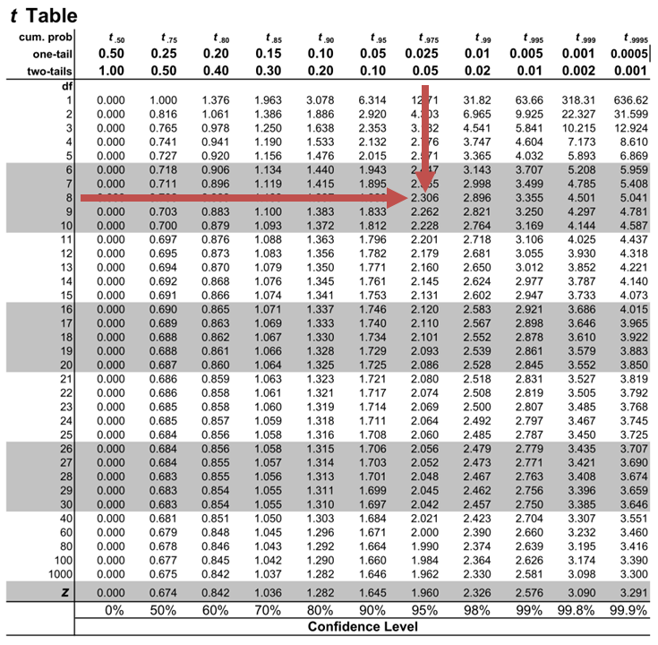
Notice that $|t|>t_{c}$ i.e., ($10.85>2.306$)

Therefore, we reject the null hypothesis and conclude that the estimated slope coefficient is statistically different from one.

Note that we used the confidence interval approach and arrived at the same conclusion.

Question Neeth Shinu, CFA, is forecasting price elasticity of supply for a certain product. Shinu uses the quantity of the product supplied for the past 5months as the dependent variable and the price per unit of the product as the independent variable. The regression results are shown below. $$\small{\begin{array}{lccccc}\hline \textbf{Regression Statistics} & & & & & \\ \hline \text{Multiple R} & 0.9971 & {}& {}&{}\\ \text{R Square} & 0.9941 & & & \\ \text{Adjusted R Square} & 0.9922 & & & & \\ \text{Standard Error} & 3.6515 & & & \\ \text{Observations} & 5 & & & \\ \hline {}& \textbf{Coefficients} & \textbf{Standard Error} & \textbf{t Stat} & \textbf{P-value}\\ \hline\text{Intercept} & -159 & 10.520 & (15.114) & 0.001\\ \text{Slope} & 0.26 & 0.012 & 22.517 & 0.000\\ \hline\end{array}}$$ Which of the following most likely reports the correct value of the t-statistic for the slope and most accurately evaluates its statistical significance with 95% confidence? A. $t=21.67$; slope is significantly different from zero. B. $t= 3.18$; slope is significantly different from zero. C. $t=22.57$; slope is not significantly different from zero. Solution The correct answer is A . The t-statistic is calculated using the formula: $$\text{t}=\frac{\widehat{b_{1}}-b_1}{\widehat{S_{b_{1}}}}$$ Where: $b_{1}$ = True slope coefficient $\widehat{b_{1}}$ = Point estimator for $b_{1}$ $\widehat{S_{b_{1}}}$ = Standard error of the regression coefficient $$\begin{align*}\text{t}&=\frac{0.26-0}{0.012}\\&=21.67\end{align*}$$ The critical two-tail t-values from the t-table with $n-2 = 3$ degrees of freedom are: $$t_{c}=±3.18$$ Notice that $|t|>t_{c}$ (i.e $21.67>3.18$). Therefore, the null hypothesis can be rejected. Further, we can conclude that the estimated slope coefficient is statistically different from zero.

Offered by AnalystPrep

Analysis of Variance (ANOVA)

Predicted value of a dependent variable, annualized returns.

To compare returns over different timeframes, we need to annualize them. This means... Read More

Point Estimate vs. Confidence Interval ...

Point Estimate A point estimate gives statisticians a single value as the estimate... Read More

Data Organization for Quantitative Ana ...

Typically, raw data can be organized into the following two formats for quantitative... Read More

Correlation

Covariance Covariance is a measure of how two variables move together. The sample... Read More

school Campus Bookshelves
menu_book Bookshelves
perm_media Learning Objects
login Login
how_to_reg Request Instructor Account
hub Instructor Commons

Margin Size

Download Page (PDF)
Download Full Book (PDF)
Periodic Table
Physics Constants
Scientific Calculator
Reference & Cite
Tools expand_more
Readability

selected template will load here

This action is not available.

16.3: The Process of Null Hypothesis Testing

Last updated
Save as PDF
Page ID 8804

Russell A. Poldrack
Stanford University

$ \newcommand{\vecs}[1]{\overset { \scriptstyle \rightharpoonup} {\mathbf{#1}} } $

$ \newcommand{\vecd}[1]{\overset{-\!-\!\rightharpoonup}{\vphantom{a}\smash {#1}}} $

$ \newcommand{\id}{\mathrm{id}}$ $ \newcommand{\Span}{\mathrm{span}}$

( \newcommand{\kernel}{\mathrm{null}\,}\) $ \newcommand{\range}{\mathrm{range}\,}$

$ \newcommand{\RealPart}{\mathrm{Re}}$ $ \newcommand{\ImaginaryPart}{\mathrm{Im}}$

$ \newcommand{\Argument}{\mathrm{Arg}}$ $ \newcommand{\norm}[1]{\| #1 \|}$

$ \newcommand{\inner}[2]{\langle #1, #2 \rangle}$

$ \newcommand{\Span}{\mathrm{span}}$

$ \newcommand{\id}{\mathrm{id}}$

$ \newcommand{\kernel}{\mathrm{null}\,}$

$ \newcommand{\range}{\mathrm{range}\,}$

$ \newcommand{\RealPart}{\mathrm{Re}}$

$ \newcommand{\ImaginaryPart}{\mathrm{Im}}$

$ \newcommand{\Argument}{\mathrm{Arg}}$

$ \newcommand{\norm}[1]{\| #1 \|}$

$ \newcommand{\Span}{\mathrm{span}}$ $ \newcommand{\AA}{\unicode[.8,0]{x212B}}$

$ \newcommand{\vectorA}[1]{\vec{#1}} % arrow$

$ \newcommand{\vectorAt}[1]{\vec{\text{#1}}} % arrow$

$ \newcommand{\vectorB}[1]{\overset { \scriptstyle \rightharpoonup} {\mathbf{#1}} } $

$ \newcommand{\vectorC}[1]{\textbf{#1}} $

$ \newcommand{\vectorD}[1]{\overrightarrow{#1}} $

$ \newcommand{\vectorDt}[1]{\overrightarrow{\text{#1}}} $

$ \newcommand{\vectE}[1]{\overset{-\!-\!\rightharpoonup}{\vphantom{a}\smash{\mathbf {#1}}}} $

We can break the process of null hypothesis testing down into a number of steps:

Formulate a hypothesis that embodies our prediction ( before seeing the data )
Collect some data relevant to the hypothesis
Specify null and alternative hypotheses
Fit a model to the data that represents the alternative hypothesis and compute a test statistic
Compute the probability of the observed value of that statistic assuming that the null hypothesis is true
Assess the “statistical significance” of the result

For a hands-on example, let’s use the NHANES data to ask the following question: Is physical activity related to body mass index? In the NHANES dataset, participants were asked whether they engage regularly in moderate or vigorous-intensity sports, fitness or recreational activities (stored in the variable P h y s A c t i v e PhysActive ). The researchers also measured height and weight and used them to compute the Body Mass Index (BMI):

B M I = w e i g h t ( k g ) h e i g h t ( m ) 2 BMI = \frac{weight(kg)}{height(m)^2}

16.3.1 Step 1: Formulate a hypothesis of interest

For step 1, we hypothesize that BMI is greater for people who do not engage in physical activity, compared to those who do.

16.3.2 Step 2: Collect some data

For step 2, we collect some data. In this case, we will sample 250 individuals from the NHANES dataset. Figure 16.1 shows an example of such a sample, with BMI shown separately for active and inactive individuals.

Box plot of BMI data from a sample of adults from the NHANES dataset, split by whether they reported engaging in regular physical activity.

16.3.3 Step 3: Specify the null and alternative hypotheses

For step 3, we need to specify our null hypothesis (which we call H 0 H _0 ) and our alternative hypothesis (which we call H A H_A ). H 0 H _0 is the baseline against which we test our hypothesis of interest: that is, what would we expect the data to look like if there was no effect? The null hypothesis always involves some kind of equality (=, ≤ \le , or ≥ \ge ). H A H_A describes what we expect if there actually is an effect. The alternative hypothesis always involves some kind of inequality ( ≠ \ne , >, or <). Importantly, null hypothesis testing operates under the assumption that the null hypothesis is true unless the evidence shows otherwise.

We also have to decide whether to use directional or non-directional hypotheses. A non-directional hypothesis simply predicts that there will be a difference, without predicting which direction it will go. For the BMI/activity example, a non-directional null hypothesis would be:

H 0 : B M I a c t i v e = B M I i n a c t i v e H0 : BMI_{active} = BMI_{inactive}

and the corresponding non-directional alternative hypothesis would be:

H A : B M I a c t i v e ≠ B M I i n a c t i v e HA: BMI_{active} \neq BMI_{inactive}

A directional hypothesis, on the other hand, predicts which direction the difference would go. For example, we have strong prior knowledge to predict that people who engage in physical activity should weigh less than those who do not, so we would propose the following directional null hypothesis:

H 0 : B M I a c t i v e ≥ B M I i n a c t i v e H0: BMI_{active} \ge BMI_{inactive}

and directional alternative:

H A : B M I a c t i v e < B M I i n a c t i v e HA : BMI_{active} < BMI_{inactive}

As we will see later, testing a non-directional hypothesis is more conservative, so this is generally to be preferred unless there is a strong a priori reason to hypothesize an effect in a particular direction. Any direction hypotheses should be specified prior to looking at the data!

16.3.4 Step 4: Fit a model to the data and compute a test statistic

For step 4, we want to use the data to compute a statistic that will ultimately let us decide whether the null hypothesis is rejected or not. To do this, the model needs to quantify the amount of evidence in favor of the alternative hypothesis, relative to the variability in the data. Thus we can think of the test statistic as providing a measure of the size of the effect compared to the variability in the data. In general, this test statistic will have a probability distribution associated with it, because that allows us to determine how likely our observed value of the statistic is under the null hypothesis.

For the BMI example, we need a test statistic that allows us to test for a difference between two means, since the hypotheses are stated in terms of mean BMI for each group. One statistic that is often used to compare two means is the t-statistic , first developed by the statistician William Sealy Gossett, who worked for the Guiness Brewery in Dublin and wrote under the pen name “Student” - hence, it is often called “Student’s t-statistic”. The t-statistic is appropriate for comparing the means of two groups when the sample sizes are relatively small and the population standard deviation is unknown. The t-statistic for comparison of two independent groups is computed as:

t = X 1 ‾ − X 2 ‾ S 1 2 n 1 + S 2 2 n 2 t = \frac{\bar{X_1} - \bar{X_2}}{\sqrt{\frac{S_1^2}{n_1} + \frac{S_2^2}{n_2}}}

where X ‾ 1 \bar{X}_1 and X ‾ 2 \bar{X}_2 are the means of the two groups, S 1 2 S ^2_1 and S 2 2 S ^2_2 are the estimated variances of the groups, and n 1 n _1 and n 2 n _2 are the sizes of the two groups. Note that the denominator is basically an average of the standard error of the mean for the two samples. Thus, one can view the the t-statistic as a way of quantifying how large the difference between groups is in relation to the sampling variability of the means that are being compared.

The t-statistic is distributed according to a probability distribution known as a t distribution. The t distribution looks quite similar to a normal distribution, but it differs depending on the number of degrees of freedom, which for this example is the number of observations minus 2, since we have computed two means and thus given up two degrees of freedom. When the degrees of freedom are large (say 1000), then the t distribution looks essentialy like the normal distribution, but when they are small then the t distribution has longer tails than the normal (see Figure 16.2).

Each panel shows the t distribution (in blue dashed line) overlaid on the normal distribution (in solid red line). The left panel shows a t distribution with 4 degrees of freedom, in which case the distribution is similar but has slightly wider tails. The right panel shows a t distribution with 1000 degrees of freedom, in which case it is virtually identical to the normal.

16.3.5 Step 5: Determine the probability of the data under the null hypothesis

This is the step where NHST starts to violate our intuition – rather than determining the likelihood that the null hypothesis is true given the data, we instead determine the likelihood of the data under the null hypothesis - because we started out by assuming that the null hypothesis is true! To do this, we need to know the probability distribution for the statistic under the null hypothesis, so that we can ask how likely the data are under that distribution. Before we move to our BMI data, let’s start with some simpler examples.

16.3.5.1 Randomization: A very simple example

Let’s say that we wish to determine whether a coin is fair. To collect data, we flip the coin 100 times, and we count 70 heads. In this example, H 0 : P ( h e a d s ) = 0.5 H_0: P(heads)=0.5 and H A : P ( h e a d s ) ≠ 0.5 H_A: P(heads) \neq 0.5 , and our test statistic is simply the number of heads that we counted. The question that we then want to ask is: How likely is it that we would observe 70 heads if the true probability of heads is 0.5. We can imagine that this might happen very occasionally just by chance, but doesn’t seem very likely. To quantify this probability, we can use the binomial distribution :

P ( X < k ) = ∑ i = 0 k ( N k ) p i ( 1 − p ) ( n − i ) P(X < k) = \sum_{i=0}^k \binom{N}{k} p^i (1-p)^{(n-i)} This equation will tell us the likelihood of a certain number of heads or fewer, given a particular probability of heads. However, what we really want to know is the probability of a certain number or more, which we can obtain by subtracting from one, based on the rules of probability:

P ( X ≥ k ) = 1 − P ( X < k ) P(X \ge k) = 1 - P(X < k)

Distribution of numbers of heads (out of 100 flips) across 100,000 simulated runsl with the observed value of 70 flips represented by the vertical line.

We can compute the probability for our example using the pbinom() function. The probability of 69 or fewer heads given P(heads)=0.5 is 0.999961, so the probability of 70 or more heads is simply one minus that value (0.000039) This computation shows us that the likelihood of getting 70 heads if the coin is indeed fair is very small.

Now, what if we didn’t have the pbinom() function to tell us the probability of that number of heads? We could instead determine it by simulation – we repeatedly flip a coin 100 times using a true probability of 0.5, and then compute the distribution of the number of heads across those simulation runs. Figure 16.3 shows the result from this simulation. Here we can see that the probability computed via simulation (0.000030) is very close to the theoretical probability (.00004).

Let’s do the analogous computation for our BMI example. First we compute the t statistic using the values from our sample that we calculated above, where we find that (t = 3.86). The question that we then want to ask is: What is the likelihood that we would find a t statistic of this size, if the true difference between groups is zero or less (i.e. the directional null hypothesis)?

We can use the t distribution to determine this probability. Our sample size is 250, so the appropriate t distribution has 248 degrees of freedom because lose one for each of the two means that we computed. We can use the pt() function in R to determine the probability of finding a value of the t-statistic greater than or equal to our observed value. Note that we want to know the probability of a value greater than our observed value, but by default pt() gives us the probability of a value less than the one that we provide it, so we have to tell it explicitly to provide us with the “upper tail” probability (by setting lower.tail = FALSE ). We find that (p(t > 3.86, df = 248) = 0.000), which tells us that our observed t-statistic value of 3.86 is relatively unlikely if the null hypothesis really is true.

In this case, we used a directional hypothesis, so we only had to look at one end of the null distribution. If we wanted to test a non-directional hypothesis, then we would need to be able to identify how unexpected the size of the effect is, regardless of its direction. In the context of the t-test, this means that we need to know how likely it is that the statistic would be as extreme in either the positive or negative direction. To do this, we multiply the observed t value by -1, since the t distribution is centered around zero, and then add together the two tail probabilities to get a two-tailed p-value: (p(t > 3.86 or t< -3.86, df = 248) = 0.000). Here we see that the p value for the two-tailed test is twice as large as that for the one-tailed test, which reflects the fact that an extreme value is less surprising since it could have occurred in either direction.

How do you choose whether to use a one-tailed versus a two-tailed test? The two-tailed test is always going to be more conservative, so it’s always a good bet to use that one, unless you had a very strong prior reason for using a one-tailed test. In that case, you should have written down the hypothesis before you ever looked at the data. In Chapter 32 we will discuss the idea of pre-registration of hypotheses, which formalizes the idea of writing down your hypotheses before you ever see the actual data. You should never make a decision about how to perform a hypothesis test once you have looked at the data, as this can introduce serious bias into the results.

16.3.5.2 Computing p-values using randomization

So far we have seen how we can use the t-distribution to compute the probability of the data under the null hypothesis, but we can also do this using simulation. The basic idea is that we generate simulated data like those that we would expect under the null hypothesis, and then ask how extreme the observed data are in comparison to those simulated data. The key question is: How can we generate data for which the null hypothesis is true? The general answer is that we can randomly rearrange the data in a particular way that makes the data look like they would if the null was really true. This is similar to the idea of bootstrapping, in the sense that it uses our own data to come up with an answer, but it does it in a different way.

16.3.5.3 Randomization: a simple example

Let’s start with a simple example. Let’s say that we want to compare the mean squatting ability of football players with cross-country runners, with H 0 : μ F B ≤ μ X C H_0: \mu_{FB} \le \mu_{XC} and H A : μ F B > μ X C H _A: \mu_{FB} > \mu_{XC} . We measure the maximum squatting ability of 5 football players and 5 cross-country runners (which we will generate randomly, assuming that μ F B = 300 \mu_{FB} = 300 , μ X C = 140 \mu_{XC} = 140 , and σ = 30 \sigma = 30 ).

Left: Box plots of simulated squatting ability for football players and cross-country runners.Right: Box plots for subjects assigned to each group after scrambling group labels.

From the plot in Figure 16.4 it’s clear that there is a large difference between the two groups. We can do a standard t-test to test our hypothesis, using the t.test() command in R, which gives the following result:

If we look at the p-value reported here, we see that the likelihood of such a difference under the null hypothesis is very small, using the t distribution to define the null.

Now let’s see how we could answer the same question using randomization. The basic idea is that if the null hypothesis of no difference between groups is true, then it shouldn’t matter which group one comes from (football players versus cross-country runners) – thus, to create data that are like our actual data but also conform to the null hypothesis, we can randomly reorder the group labels for the individuals in the dataset, and then recompute the difference between the groups. The results of such a shuffle are shown in Figure ?? .

Histogram of t-values for the difference in means between the football and cross-country groups after randomly shuffling group membership. The vertical line denotes the actual difference observed between the two groups, and the dotted line shows the theoretical t distribution for this analysis.

After scrambling the labels, we see that the two groups are now much more similar, and in fact the cross-country group now has a slightly higher mean. Now let’s do that 10000 times and store the t statistic for each iteration; this may take a moment to complete. Figure 16.5 shows the histogram of the t-values across all of the random shuffles. As expected under the null hypothesis, this distribution is centered at zero (the mean of the distribution is -0.016. From the figure we can also see that the distribution of t values after shuffling roughly follows the theoretical t distribution under the null hypothesis (with mean=0), showing that randomization worked to generate null data. We can compute the p-value from the randomized data by measuring how many of the shuffled values are at least as extreme as the observed value: p(t > 5.14, df = 8) using randomization = 0.00380. This p-value is very similar to the p-value that we obtained using the t distribution, and both are quite extreme, suggesting that the observed data are very unlikely to have arisen if the null hypothesis is true - and in this case we know that it’s not true, because we generated the data.

16.3.5.3.1 Randomization: BMI/activity example

Now let’s use randomization to compute the p-value for the BMI/activity example. In this case, we will randomly shuffle the PhysActive variable and compute the difference between groups after each shuffle, and then compare our observed t statistic to the distribution of t statistics from the shuffled datasets. Figure 16.6 shows the distribution of t values from the shuffled samples, and we can also compute the probability of finding a value as large or larger than the observed value. The p-value obtained from randomization (0.0000) is very similar to the one obtained using the t distribution (0.0001). The advantage of the randomization test is that it doesn’t require that we assume that the data from each of the groups are normally distributed, though the t-test is generally quite robust to violations of that assumption. In addition, the randomization test can allow us to compute p-values for statistics when we don’t have a theoretical distribution like we do for the t-test.

Histogram of t statistics after shuffling of group labels, with the observed value of the t statistic shown in the vertical line, and values at least as extreme as the observed value shown in lighter gray

We do have to make one main assumption when we use the randomization test, which we refer to as exchangeability . This means that all of the observations are distributed in the same way, such that we can interchange them without changing the overall distribution. The main place where this can break down is when there are related observations in the data; for example, if we had data from individuals in 4 different families, then we couldn’t assume that individuals were exchangeable, because siblings would be closer to each other than they are to individuals from other families. In general, if the data were obtained by random sampling, then the assumption of exchangeability should hold.

16.3.6 Step 6: Assess the “statistical significance” of the result

The next step is to determine whether the p-value that results from the previous step is small enough that we are willing to reject the null hypothesis and conclude instead that the alternative is true. How much evidence do we require? This is one of the most controversial questions in statistics, in part because it requires a subjective judgment – there is no “correct” answer.

Historically, the most common answer to this question has been that we should reject the null hypothesis if the p-value is less than 0.05. This comes from the writings of Ronald Fisher, who has been referred to as “the single most important figure in 20th century statistics” (Efron 1998) :

“If P is between .1 and .9 there is certainly no reason to suspect the hypothesis tested. If it is below .02 it is strongly indicated that the hypothesis fails to account for the whole of the facts. We shall not often be astray if we draw a conventional line at .05 … it is convenient to draw the line at about the level at which we can say: Either there is something in the treatment, or a coincidence has occurred such as does not occur more than once in twenty trials” (Fisher 1925)

However, Fisher never intended p < 0.05 p < 0.05 to be a fixed rule:

“no scientific worker has a fixed level of significance at which from year to year, and in all circumstances, he rejects hypotheses; he rather gives his mind to each particular case in the light of his evidence and his ideas” [fish:1956]

Instead, it is likely that it became a ritual due to the reliance upon tables of p-values that were used before computing made it easy to compute p values for arbitrary values of a statistic. All of the tables had an entry for 0.05, making it easy to determine whether one’s statistic exceeded the value needed to reach that level of significance.

The choice of statistical thresholds remains deeply controversial, and recently (Benjamin et al., 2018) it has been proposed that the standard threshold be changed from .05 to .005, making it substantially more stringent and thus more difficult to reject the null hypothesis. In large part this move is due to growing concerns that the evidence obtained from a significant result at p < . 05 32.

16.3.6.1 Hypothesis testing as decision-making: The Neyman-Pearson approach

Whereas Fisher thought that the p-value could provide evidence regarding a specific hypothesis, the statisticians Jerzy Neyman and Egon Pearson disagreed vehemently. Instead, they proposed that we think of hypothesis testing in terms of its error rate in the long run:

“no test based upon a theory of probability can by itself provide any valuable evidence of the truth or falsehood of a hypothesis. But we may look at the purpose of tests from another viewpoint. Without hoping to know whether each separate hypothesis is true or false, we may search for rules to govern our behaviour with regard to them, in following which we insure that, in the long run of experience, we shall not often be wrong” (Neyman and Pearson 1933)

That is: We can’t know which specific decisions are right or wrong, but if we follow the rules, we can at least know how often our decisions will be wrong on average.

To understand the decision making framework that Neyman and Pearson developed, we first need to discuss statistical decision making in terms of the kinds of outcomes that can occur. There are two possible states of reality ( H 0 H _0 is true, or H 0 H _0 is false), and two possible decisions (reject H 0 H _0 , or fail to reject H 0 H _0 ). There are two ways in which we can make a correct decision:

We can decide to reject H 0 H _0 when it is false (in the language of decision theory, we call this a hit )
We can fail to reject H 0 H _0 when it is true (we call this a correct rejection )

There are also two kinds of errors we can make:

We can decide to reject H 0 H _0 when it is actually true (we call this a false alarm , or Type I error )
We can fail to reject H 0 H _0 when it is actually false (we call this a miss , or Type II error )

Neyman and Pearson coined two terms to describe the probability of these two types of errors in the long run:

P(Type I error) = α \alpha
P(Type II error) = β \beta

That is, if we set α 18.3, which is the complement of Type II error.

16.3.7 What does a significant result mean?

There is a great deal of confusion about what p-values actually mean (Gigerenzer, 2004). Let’s say that we do an experiment comparing the means between conditions, and we find a difference with a p-value of .01. There are a number of possible interpretations.

16.3.7.1 Does it mean that the probability of the null hypothesis being true is .01?

No. Remember that in null hypothesis testing, the p-value is the probability of the data given the null hypothesis ( P ( d a t a | H 0 ) P(data|H_0) ). It does not warrant conclusions about the probability of the null hypothesis given the data ( P ( H 0 | d a t a ) P(H_0|data) ). We will return to this question when we discuss Bayesian inference in a later chapter, as Bayes theorem lets us invert the conditional probability in a way that allows us to determine the latter probability.

16.3.7.2 Does it mean that the probability that you are making the wrong decision is .01?

No. This would be P ( H 0 | d a t a ) P(H_0|data) , but remember as above that p-values are probabilities of data under H 0 H _0 , not probabilities of hypotheses.

16.3.7.3 Does it mean that if you ran the study again, you would obtain the same result 99% of the time?

No. The p-value is a statement about the likelihood of a particular dataset under the null; it does not allow us to make inferences about the likelihood of future events such as replication.

16.3.7.4 Does it mean that you have found a meaningful effect?

No. There is an important distinction between statistical significance and practical significance . As an example, let’s say that we performed a randomized controlled trial to examine the effect of a particular diet on body weight, and we find a statistically significant effect at p<.05. What this doesn’t tell us is how much weight was actually lost, which we refer to as the effect size (to be discussed in more detail in Chapter 18). If we think about a study of weight loss, then we probably don’t think that the loss of ten ounces (i.e. the weight of a bag of potato chips) is practically significant. Let’s look at our ability to detect a significant difference of 1 ounce as the sample size increases.

Figure 16.7 shows how the proportion of significant results increases as the sample size increases, such that with a very large sample size (about 262,000 total subjects), we will find a significant result in more than 90% of studies when there is a 1 ounce weight loss. While these are statistically significant, most physicians would not consider a weight loss of one ounce to be practically or clinically significant. We will explore this relationship in more detail when we return to the concept of statistical power in Section 18.3, but it should already be clear from this example that statistical significance is not necessarily indicative of practical significance.

The proportion of signifcant results for a very small change (1 ounce, which is about .001 standard deviations) as a function of sample size.

IMAGES

PPT
Hypothesis Test for Simple Linear Regession
Mod-01 Lec-39 Hypothesis Testing in Linear Regression
Understanding the Null Hypothesis for Linear Regression
Null Hypothesis Significance Testing Overview
Explaining Linear Regression With Hypothesis Testing And

VIDEO

Null Hypothesis Test Examples
Hypothesis testing
Statistics and probability
Hypothesis Tests for One Sample Mean Using Excel Companion Workbook
SPSS-10: Hypothesis testing using regression (Urdu/Hindi)
Multiple Regression and Hypothesis Testing

COMMENTS

Understanding the Null Hypothesis for Linear Regression
xi: The value of the predictor variable xi. Multiple linear regression uses the following null and alternative hypotheses: H0: β1 = β2 = … = βk = 0. HA: β1 = β2 = … = βk ≠ 0. The null hypothesis states that all coefficients in the model are equal to zero. In other words, none of the predictor variables have a statistically ...
12.2.1: Hypothesis Test for Linear Regression
The null hypothesis of a two-tailed test states that there is not a linear relationship between $x$ and $y$. ... T-Test for Regression. If the regression equation has a slope of zero, then every $x$ value will give the same $y$ value and the regression equation would be useless for prediction. We should perform a t-test to see if the ...
15.5: Hypothesis Tests for Regression Models
Testing the model as a whole. Okay, suppose you've estimated your regression model. The first hypothesis test you might want to try is one in which the null hypothesis that there is no relationship between the predictors and the outcome, and the alternative hypothesis is that the data are distributed in exactly the way that the regression model predicts.
13.6 Testing the Regression Coefficients
The hypothesis test for a regression coefficient is a well established process: Write down the null and alternative hypotheses in terms of the regression coefficient being tested. The null hypothesis is the claim that there is no relationship between the dependent variable and independent variable.
3.3.4: Hypothesis Test for Simple Linear Regression
In simple linear regression, this is equivalent to saying "Are X an Y correlated?". In reviewing the model, Y = β0 +β1X + ε Y = β 0 + β 1 X + ε, as long as the slope ( β1 β 1) has any non‐zero value, X X will add value in helping predict the expected value of Y Y. However, if there is no correlation between X and Y, the value of ...
Null Hypothesis: Definition, Rejecting & Examples
Null Hypothesis H 0: The correlation in the population is zero: ρ = 0. Alternative Hypothesis H A: The correlation in the population is not zero: ρ ≠ 0. For all these cases, the analysts define the hypotheses before the study. After collecting the data, they perform a hypothesis test to determine whether they can reject the null hypothesis.
Understanding the Null Hypothesis for Linear Regression
Multiple linear regression uses the following null and alternative hypotheses: H 0: β 1 = β 2 = … = β k = 0; H A: β 1 = β 2 = … = β k ≠ 0; The null hypothesis states that all coefficients in the model are equal to zero. In other words, none of the predictor variables have a statistically significant relationship with the response ...
PDF Chapter 9 Simple Linear Regression
218 CHAPTER 9. SIMPLE LINEAR REGRESSION 9.2 Statistical hypotheses For simple linear regression, the chief null hypothesis is H 0: β 1 = 0, and the corresponding alternative hypothesis is H 1: β 1 6= 0. If this null hypothesis is true, then, from E(Y) = β 0 + β 1x we can see that the population mean of Y is β 0 for
Linear regression
The null hypothesis is rejected if falls outside the acceptance region. How the acceptance region is determined depends not only on the desired size of the test, but also on whether the test is: two-tailed (could be smaller or larger than ; we do not exclude either of the two possibilities) . one-tailed (only one of the two things, i.e., either smaller or larger, is possible).
6.4
The reduced model is the model that the null hypothesis describes. Because the null hypothesis sets each of the slope parameters in the full model equal to 0, the reduced model is: ... But, note that we've just learned something new about the meaning of the t-test in the multiple regression setting. It tests for the ("marginal") significance of ...
PDF Lecture 5 Hypothesis Testing in Multiple Linear Regression
As in simple linear regression, under the null hypothesis t 0 = βˆ j seˆ(βˆ j) ∼ t n−p−1. We reject H 0 if |t 0| > t n−p−1,1−α/2. This is a partial test because βˆ j depends on all of the other predictors x i, i 6= j that are in the model. Thus, this is a test of the contribution of x j given the other predictors in the model.
Null & Alternative Hypotheses
Research question: Null hypothesis (H 0): General: Test-specific: Does tooth flossing affect the number of cavities? Tooth flossing has no effect on the number of cavities.: t test:. The mean number of cavities per person does not differ between the flossing group (µ 1) and the non-flossing group (µ 2) in the population; µ 1 = µ 2.: Does the amount of text highlighted in the textbook ...
What is a null model in regression and how does it relate to the null
$\begingroup$ The null hypothesis is usually something specific about parameter values; I'd say the null model would be the null hypothesis plus all the accompanying assumptions under which the null distribution of the test statistic would be derived-- its the assumptions that contain most of the model.For example the null hypothesis doesn't mention independence, but I'd definitely say it's ...
Linear regression hypothesis testing: Concepts, Examples
Thus, the null hypothesis is set that there is no relationship between response and the predictor variables. Hence, the coefficients related to each of the predictor variables is equal to zero (0). So, if the linear regression model is Y = a0 + a1x1 + a2x2 + a3x3, then the null hypothesis for each test states that a1 = 0, a2 = 0, a3 = 0 etc.
11.1: Testing the Hypothesis that β = 0
METHOD 1: Using a p-value to make a decision. To calculate the p-value using LinRegTTEST: On the LinRegTTEST input screen, on the line prompt for β or ρ, highlight " ≠ 0 ". The output screen shows the p-value on the line that reads " p = ". (Most computer statistical software can calculate the p-value .)
6.2.3
This is like the overall F−test in linear regression. In other words, this is testing the null hypothesis of the intercept-only model: $\log\left(\dfrac{\pi}{1-\pi}\right)=\beta_0$ versus the alternative that the current (full) model is correct. This corresponds to the test in our example because we have only a single predictor term, and ...
Hypothesis Test for Regression Slope
Hypothesis Test for Regression Slope. This lesson describes how to conduct a hypothesis test to determine whether there is a significant linear relationship between an independent variable X and a dependent variable Y.. The test focuses on the slope of the regression line Y = Β 0 + Β 1 X. where Β 0 is a constant, Β 1 is the slope (also called the regression coefficient), X is the value of ...
Hypothesis Testing in Regression Analysis
Reject the null hypothesis if the absolute value of the t-statistic is greater than the critical t-value i.e., $t\ >\ +\ t_{critical}\ or\ t\ <\ -t_{\text{critical}}$. Example: Hypothesis Testing of the Significance of Regression Coefficients. An analyst generates the following output from the regression analysis of inflation on unemployment:
How to Interpret the F-test of Overall Significance in Regression
If a p-value equals one, then you know that the sample data exactly equal the null hypothesis condition. Your p-value is 0.99, so you know that the sample data almost exactly equals the null hypothesis value. For one-way ANOVA, the null hypothesis states that all group means are equal. So, your sample means must be almost exactly equal.
PDF Hypothesis Testing in the Multiple regression model
- The errors in the regression equaion are distributed normally. In this case we can show that under the null hypothesis H0 the F-statistic is distributed as an F distribution with degrees of freedom (q,N-k) . - The number of restrictions q are the degrees of freedom of the numerator. - N-K are the degrees of freedom of the denominator.
16.3: The Process of Null Hypothesis Testing
16.3.5 Step 5: Determine the probability of the data under the null hypothesis. This is the step where NHST starts to violate our intuition - rather than determining the likelihood that the null hypothesis is true given the data, we instead determine the likelihood of the data under the null hypothesis - because we started out by assuming that the null hypothesis is true!
PDF Lecture 13 Estimation and hypothesis testing for logistic regression
Score test If the MLE equals the hypothesized value, p 0, then p 0 would maximize the likelihood and U(p 0) = 0. The score statistic measures how far from zero the score function is when evaluated at the null hypothesis. The test statistic for the binary outcome example is S = U(p 0)2/I(p 0), and S ∼ χ2 with 1 degree of freedom. BIOST 515 ...
Unlocking Regression Analysis: Hypothesis Testing in BI
1 Hypothesis Basics. Hypothesis testing in regression analysis begins with two basic hypotheses: the null hypothesis (H0) and the alternative hypothesis (H1). The null hypothesis states that there ...
. You are testing the null hypothesis that there is no
Since the test is two-tailed, there will be two critical values the positive and negative. Given these, the answers are: The lower critical value is -2.1009. The upper critical value is 2.1009. To determine the decision, the rules are given below. If the t-stat is inside the critical values, do not reject the null hypothesis, the result is not ...

Understanding the Null Hypothesis for Linear Regression

Example 1: Simple Linear Regression

Example 2: Multiple Linear Regression

Additional Resources

Featured Posts

2 Replies to “Understanding the Null Hypothesis for Linear Regression”

Leave a Reply Cancel reply

Join the Statology Community

13.6 Testing the Regression Coefficients

Testing the Regression Coefficients

Steps to Conduct a Hypothesis Test on a Regression Coefficient

Concept Review

Understanding the Null Hypothesis for Linear Regression

Example 1: Simple Linear Regression

Example 2: Multiple Linear Regression

Additional Resources

The Complete Guide: How to Report Regression Results

Linear regression - Hypothesis testing

Normal vs non-normal model

How to cite

Linear regression hypothesis testing: Concepts, Examples

What are linear regression models?

Train a Multiple Linear Regression Model using R

Hypothesis tests & Linear Regression Models

Why hypothesis tests for linear regression models?

Recent Posts

Ajitesh Kumar

Leave a Reply Cancel reply

ChatGPT Prompts (250+)

Data Science / AI Trends

Free Online Tools

Recent Comments

User Preferences

Keyboard Shortcuts

Testing the Joint Significance of All Predictors Section

The Homer-Lemeshow Statistic Section

Residuals Section

Hypothesis Test for Regression Slope

Test Requirements

State the Hypotheses

Formulate an Analysis Plan

Analyze Sample Data

Interpret Results

Test Your Understanding

Hypothesis Testing in Regression Analysis

The t-test Approach

Example: Hypothesis Testing of the Significance of Regression Coefficients

Analysis of Variance (ANOVA)

Point Estimate vs. Confidence Interval ...

Data Organization for Quantitative Ana ...

Correlation

Margin Size

16.3: The Process of Null Hypothesis Testing

16.3.1 Step 1: Formulate a hypothesis of interest

16.3.2 Step 2: Collect some data

16.3.3 Step 3: Specify the null and alternative hypotheses

16.3.4 Step 4: Fit a model to the data and compute a test statistic

16.3.5 Step 5: Determine the probability of the data under the null hypothesis

16.3.5.1 Randomization: A very simple example

16.3.5.2 Computing p-values using randomization

16.3.5.3 Randomization: a simple example

16.3.5.3.1 Randomization: BMI/activity example

16.3.6 Step 6: Assess the “statistical significance” of the result

16.3.6.1 Hypothesis testing as decision-making: The Neyman-Pearson approach

16.3.7 What does a significant result mean?

16.3.7.1 Does it mean that the probability of the null hypothesis being true is .01?

16.3.7.2 Does it mean that the probability that you are making the wrong decision is .01?

16.3.7.3 Does it mean that if you ran the study again, you would obtain the same result 99% of the time?

16.3.7.4 Does it mean that you have found a meaningful effect?

IMAGES

VIDEO

COMMENTS