constancy hypothesis biology

Thank you for visiting nature.com. You are using a browser version with limited support for CSS. To obtain the best experience, we recommend you use a more up to date browser (or turn off compatibility mode in Internet Explorer). In the meantime, to ensure continued support, we are displaying the site without styles and JavaScript.

View all journals
Explore content
About the journal
Publish with us
Sign up for alerts
Review Article
Published: 01 March 2003

The modern molecular clock

Lindell Bromham 1 &
David Penny 2

Nature Reviews Genetics volume 4 , pages 216–224 ( 2003 ) Cite this article

10k Accesses

408 Citations

69 Altmetric

Metrics details

Rates of molecular evolution can be remarkably constant over time, producing a molecular clock.

The constancy of rates was explained by the neutral theory by assuming that most changes to DNA or protein sequences are neutral — that is, driven by drift not selection.

The neutral theory has been refined to allow for the effect of population size on the chance of mutations of small selective effect being fixed in a population (the nearly neutral theory).

The molecular clock is a 'sloppy' clock: theory predicts that the rate of molecular evolution will be influenced by mutation rate, patterns of selection and population size.

Stochastic fluctuations in substitution rate over time in lineages (residual effects) make molecular date estimates imprecise.

Variation in rate between lineages can cause substantial bias in molecular date estimates.

Attempts to use molecular clocks to date evolutionary divergences must account for these sources of imprecision and bias, and variation in rates must be expressed in confidence intervals around date estimates.

The discovery of the molecular clock — a relatively constant rate of molecular evolution — provided an insight into the mechanisms of molecular evolution, and created one of the most useful new tools in biology. The unexpected constancy of rate was explained by assuming that most changes to genes are effectively neutral. Theory predicts several sources of variation in the rate of molecular evolution. However, even an approximate clock allows time estimates of events in evolutionary history, which provides a method for testing a wide range of biological hypotheses ranging from the origins of the animal kingdom to the emergence of new viral epidemics.

This is a preview of subscription content, access via your institution

Access options

Subscribe to this journal

Receive 12 print issues and online access

176,64 € per year

only 14,72 € per issue

Buy this article

Purchase on Springer Link
Instant access to full article PDF

Prices may be subject to local taxes which are calculated during checkout

The developing toolkit of continuous directed evolution

A common root for coevolution and substitution rate variability in protein sequence evolution

Molecular and evolutionary processes generating variation in gene expression

Smith, A. B. & Peterson, K. J. Dating the time of origin of major clades: molecular clocks and the fossil record. Annu. Rev. Earth Planet. Sci. 30 , 65–88 (2002). A review of the controversy surrounding dates for the Cambrian explosion of animal phyla and the early Tertiary radiation of modern mammals and birds. Written by a palaeontologist and a molecular geneticist, this review takes a critical look at the reliability of both fossil and molecular dates.

Article CAS Google Scholar

Korber, B. et al.Timing the ancestor of the HIV-1 pandemic strains. Science 288 , 1789–1796 (2000).

Article CAS PubMed Google Scholar

Zuckerkandl, E. & Pauling, L. in Horizons in Biochemistry (eds Kasha, M. & Pullman, B.) 189–225 (Academic Press, New York, 1962).

Google Scholar

Kimura, M. & Ohta, T. On the rate of molecular evolution. J. Mol. Evol. 1 , 1–17 (1971).

Dickerson, R. E. The structure of cytochrome c and rates of molecular evolution. J. Mol. Evol. 1 , 26–45 (1971).

Penny, D., McComish, B. J., Charleston, M. A. & Hendy, M. D. Mathematical elegance with biochemical realism: the covarion model of molecular evolution. J. Mol. Evol. 53 , 711–723 (2001).

Smith, N. H. & Eyre-Walker, A. Adaptive protein evolution in Drosophila . Nature 415 , 1022–1024 (2002).

King, J. L. & Jukes, T. H. Non-Darwinian evolution. Science 164 , 788–798 (1969).

Darwin, C. The Origin of Species by Means of Natural Selection 6th edn Ch. 4 64 (John Murray, London, 1872). Remarkably prescient exposition of the processes of evolution, including a pre-genetic description of the neutral theory, pre-emptively rebutting rumours that neutral evolution is 'non–Darwinian'.

Fleischer, R. C., McIntosh, C. E. & Tarr, C. L. Evolution on a volcanic conveyor belt: using phylogeographic reconstructions and K-Ar based ages of the Hawaiian islands to estimate molecular evolutionary rates. Mol. Ecol. 7 , 533–545 (1998).

Gillespie, J. H. The Causes of Molecular Evolution (Oxford University Press, Oxford, UK, 1991).

Zheng, Q. On the dispersion index of a Markovian molecular clock. Math. Biosci. 172 , 115–128 (2001). This gives a statistical view of the expected variability in rates that occur when the simple probabilistic models of molecular evolution are allowed to increase in complexity.

Bickel, D. R. Implications of fluctuations in substitution rates: impact on the uncertainty of branch lengths and on relative-rate tests. J. Mol. Evol. 50 , 381–390 (2000).

Cutler, D. J. Estimating divergence times in the presence of an overdispersed molecular clock. Mol. Biol. Evol. 17 , 1647–1660 (2000).

Bastolla, U., Porto, M., Roman, H. E. & Vendruscolo, M. Lack of self-averaging in neutral evolution of proteins. Phys. Rev. Lett. 89 , article no. 208101 (2002). This original paper follows the evolution of protein sequences that are restricted in their predicted tertiary structure. It shows, using basic biochemical principles, that the variability in rates of a molecular clock is expected to be higher than for a simple Poisson process.

Fitch, W. M. Rate of change of concomitantly variable codons. J. Mol. Evol. 1 , 84–96 (1971).

Swanson, K. W., Irwin, D. M. & Wilson, A. C. Stomach lysozyme gene of the langur monkey: tests for convergence and positive selection. J. Mol. Evol. 33 , 418–425 (1991).

Zhang, J. Z., Zhang, Y. P. & Rosenberg, H. F. Adaptive evolution of a duplicated pancreatic ribonuclease gene in a leaf-eating monkey. Nature Genet. 30 , 411–415 (2002).

Papadopoulos, D. et al. Genomic evolution during a 10,000-generation experiment with bacteria. Proc. Natl Acad. Sci. USA 96 , 3807–3812 (1999). A laboratory experiment comparing rates of morphological and molecular evolution in bacterial populations. Although adaptive phenotypic evolution was fastest at the beginning, DNA substitutions accumulated steadily through the experiment, indicating that the molecular clock is decoupled from the pace of adaptive evolution.

Article CAS PubMed PubMed Central Google Scholar

Bromham, L., Woolfit, M., Lee, M. S. Y. & Rambaut, A. Testing the relationship between morphological and molecular rates of change along phylogenies. Evolution 56 , 1921–1930 (2002).

Article PubMed Google Scholar

Wyles, J. S., Kunkel, J. G. & Wilson, A. C. Birds, behavior, and anatomical evolution. Proc. Natl Acad. Sci. USA 80 , 4394–4397 (1983).

Ohta, T. & Kimura, M. On the constancy of the evolutionary rate of cistrons. J. Mol. Evol. 1 , 18–25 (1971).

Ohta, T. Very slightly deleterious mutations and the molecular clock. J. Mol. Evol. 26 , 1–6 (1987).

Ohta, T. Near-neutrality in evolution of genes and gene regulation. Proc. Natl Acad. Sci. USA 99 , 16134–16137 (2002). The most recent exposition of the nearly-neutral model, in which the effects of weak selection depend both on the selection coefficient of the mutation and the size of the population in which the mutant occurs.

Felsenstein, J. Evolutionary trees from DNA sequences: a maximum likelihood approach. J. Mol. Evol. 17 , 368–376 (1981).

Rambaut, A. & Bromham, L. Estimating divergence dates from molecular sequences. Mol. Biol. Evol. 15 , 442–448 (1998).

Bromham, L., Rambaut, A., Fortey, R., Cooper, A. & Penny, D. Testing the Cambrian explosion hypothesis by using a molecular dating technique. Proc. Natl Acad. Sci. USA 95 , 12386–12389 (1998).

Bromham, L. D., Rambaut, A., Hendy, M. D. & Penny, D. he power of relative rates tests depends on the data. J. Mol. Evol. 50 , 296–301 (2000).

Drake, J., Charlesworth, B., Charlesworth, D. & Crow, J. Rates of spontaneous mutation. Genetics 148 , 1667–1686 (1998). Observable mutation rates, when measured per genome per generation, are remarkably similar across widely divergent organisms, indicating that natural selection might shape optimum mutation rates.

CAS PubMed PubMed Central Google Scholar

Ota, R. & Penny, D. Estimating changes in mutational mechanisms of evolution. J. Mol. Evol. (in the press).

Hart, R. W. & Setlow, R. B. Correlation between deoxyribonucleic acid excision-repair and life-span in a number of mammal species. Proc. Natl Acad. Sci. USA 71 , 2169–2173 (1974).

Li, W. -H., Ellesworth, D. L., Krushkal, J., Chang, B. H. -J. & Hewett-Emmett, D. Rates of nucleotide substitution in primates and rodents and the generation-time effect hypothesis. Mol. Phylogenet. Evol. 5 , 182–187 (1996).

Chao, L. & Cox, E. C. Competition between high and low mutating strains of Escherichia coli . Evolution 37 , 125–134 (1983).

Rand, D. M. Thermal habit, metabolic rate and the evolution of mitochondrial DNA. Trends Ecol. Evol. 9 , 125–131 (1994).

Martin, A. P. & Palumbi, S. R. Body size, metabolic rate, generation time and the molecular clock. Proc. Natl Acad. Sci. USA 90 , 4087–4091 (1993). Showed a relationship between body size and the rate of molecular evolution for vertebrates using estimates of absolute substitution rates. This paper showed that the life history of a species must influence the rate of molecular evolution.

Martin, A. P. Metabolic rate and directional nucleotide substitution in animal mitochondrial DNA. Mol. Biol. Evol. 12 , 1124–1131 (1995).

CAS PubMed Google Scholar

Bromham, L., Rambaut, A. & Harvey, P. H. Determinants of rate variation in mammalian DNA sequence evolution. J. Mol. Evol. 43 , 610–621 (1996).

Bromham, L. Molecular clocks in reptiles: life history influences rate of molecular evolution. Mol. Biol. Evol. 19 , 302–309. (2002).

Mooers, A. Ø. & Harvey, P. H. Metabolic rate, generation time and the rate of molecular evolution in birds. Mol. Phylogenet. Evol. 3 , 344–350 (1994).

Bromham, L. & Cardillo, M. Testing the link between the latitudinal gradient in species richness and rates of molecular evolution. J. Evol. Biol. 16 , 200–207 (2003).

Held, C. No evidence for slow-down of molecular substitution rates at subzero temperatures in Antarctic serolid isopods (Crustacea, Isopoda, Serolidae). Polar Biol. 24 , 497–501 (2001).

Article Google Scholar

Bielas, J. H. & Heddle, J. A. Proliferation is necessary for both repair and mutation in transgenic mouse cells. Proc. Natl Acad. Sci. USA 97 , 11391–11396 (2000).

Johnson, K. P. & Seger, J. Elevated rates of nonsynonymous substitution in island birds. Mol. Biol. Evol. 18 , 874–881 (2001).

Schmitz, J. & Moritz, R. F. A. Sociality and the rate of rDNA sequence evolution in wasps (Vespidae) and honeybees Apis . J. Mol. Evol. 47 , 606–612 (1998).

Moran, N. A. Accelerated evolution and Muller's rachet in endosymbiotic bacteria. Proc. Natl Acad. Sci. USA 93 , 2873–2878 (1996).

Barraclough, T. G. & Savolainen, V. Evolutionary rates and species diversity in flowering plants. Evolution 55 , 677–683 (2001).

Doolittle, R. F., Feng, D. F., Tsang, S., Cho, G. & Little, E. Determining divergence times of the major kingdoms of living organisms with a protein clock. Science 271 , 470–477 (1996).

Bromham, L. D., Phillips, M. J. & Penny, D. Growing up with dinosaurs: molecular dates and the mammalian radiation. Trends Ecol. Evol. 14 , 113–118 (1999).

Bromham, L. Molecular clocks and explosive radiations. J. Mol. Evol. (in the press).

Wu, C. -I. & Li, W. -H. Evidence for higher rates of nucleotide substitutions in rodents than in man. Proc. Natl Acad. Sci. USA 82 , 1741–1745 (1985).

Tajima, F. Simple methods for testing the molecular evolutionary clock hypothesis. Genetics 135 , 599–607 (1993).

Kumar, S. & Hedges, S. B. A molecular timescale for vertebrate evolution. Nature 392 , 917–920 (1998).

Nei, M. & Glazko, G. V. Estimation of divergence times for a few mammalian and several primate species. J. Hered. 93 , 157–164 (2002).

Takezaki, N., Rzhetsky, A. & Nei, M. Phylogenetic test of the molecular clock and linearized trees. Mol. Biol. Evol. 12 , 823–833 (1995).

Bromham, L. D. & Hendy, M. D. Can fast early rates reconcile molecular dates to the Cambrian explosion? Proc. R. Soc. Lond. B 267 , 1041–1047 (2000).

Sanderson, M. J. A nonparametric approach to estimating divergence times in the absence of rate constancy. J. Mol. Evol. 14 , 1218–1231 (1997).

Kishino, H., Thorne, J. L. & Bruno, W. J. Performance of a divergence time estimation method under a probabilistic model of rate evolution. Mol. Biol. Evol. 18 , 352–361 (2001). This paper outlined new Bayesian methods for estimating dates of divergence if rates of molecular evolution vary between lineages, by allowing the mutation rate to vary with time, and averages its estimates over a range of alternatives.

Aris-Brosou, S. & Yang, Z. Effects of models of rate evolution on estimation of divergence dates with special reference to the metazoan 18S ribosomal RNA phylogeny. Syst. Biol. 51 , 703–714 (2002).

Rannala, B. Identifiability of parameters in MCMC Bayesian inference of phylogeny. Syst. Biol. 51 , 754–760 (2002).

Bromham, L. The human zoo: endogenous retroviruses in the human genome. Trends Ecol. Evol. 17 , 91–97 (2002).

Tristem, M. Identification and characterization of novel human endogenous retrovirus families by phylogenetic screening of the Human Genome Mapping Project database. J. Virol. 74 , 3715–3730 (2000).

Shankarappa, R. et al. Consistent viral evolutionary changes associated with the progression of human immunodeficiency virus type 1 infection. J. Virol. 73 , 10489–10502 (1999).

Twiddy, S. S., Holmes, E. C. & Rambaut, A. Inferring the rate and time-scale of dengue virus evolution. Mol. Biol. Evol. 20 , 122–129 (2003).

Drummond, A., Pybus, O. G. & Rambaut, A. Inference of viral evolutionary rates from molecular sequences. Adv. Parasitol. (in the press). A review of the methods used to estimate substitution rates in viruses, including estimating molecular dates when rates vary.

Fitch, W. M., Leiter, J. M., Li, X. Q. & Palese, P. Positive Darwinian evolution in human influenza A viruses. Proc. Natl Acad. Sci. USA 88 , 4270–4274 (1991).

Rambaut, A. Estimating the rate of molecular evolution: incorporating non-contemporaneous sequences into maximum likelihood phylogenies. Bioinformatics 16 , 395–399 (2000).

Page, R. D. M. & Holmes, E. C. Molecular Evolution: a Phylogenetic Approach (Blackwell Science, Oxford, UK, 1998).

Madsen, O. et al.Parallel adaptive radiations in two major clades of placental mammals. Nature 409 , 610–614 (2001). Used the quartet method which uses several calibration dates to allow for differences in substitution rate between lineages to support the hypothesis that modern mammals arose long before the final extinction of the dinosaurs.

Conway Morris, S. Early metazoan evolution: reconciling paleontology and molecular biology. Am. Zool. 38 , 867–877 (1998).

Valentine, J., Jablonski, D. & Erwin, D. Fossils, molecules and embryos: new perspectives on the Cambrian explosion. Development 126 , 851–859 (1999).

Carroll, R. C. Towards a new evolutionary synthesis. Trends Ecol. Evol. 15 , 27–32 (2000).

Kimura, M. The Neutral Theory of Molecular Evolution (Cambridge University Press, Cambridge, UK, 1983).

Book Google Scholar

Download references

Acknowledgements

We thank A. Rambaut and A. Eyre-Walker for helpful comments.

Author information

Authors and affiliations.

Centre for the Study of Evolution, School of Biological Sciences, University of Sussex, Falmer, BN1 9QG, Brighton, UK

Lindell Bromham

Allan Wilson Centre for Molecular Ecology and Evolution, Massey University, Palmerston North, New Zealand

David Penny

You can also search for this author in PubMed Google Scholar

Corresponding author

Correspondence to Lindell Bromham .

Rights and permissions

Reprints and permissions

About this article

Cite this article.

Bromham, L., Penny, D. The modern molecular clock . Nat Rev Genet 4 , 216–224 (2003). https://doi.org/10.1038/nrg1020

Download citation

Issue Date : 01 March 2003

DOI : https://doi.org/10.1038/nrg1020

Share this article

Anyone you share the following link with will be able to read this content:

Sorry, a shareable link is not currently available for this article.

Provided by the Springer Nature SharedIt content-sharing initiative

This article is cited by

Speciation and historical migration pattern interaction: examples from p. nigra and p. sylvestris phylogeography.

Krassimir D. Naydenov
Michel K. Naydenov
Faruk Bogunic

European Journal of Forest Research (2023)

Base-substitution mutation rate across the nuclear genome of Alpheus snapping shrimp and the timing of isolation by the Isthmus of Panama

Katherine Silliman
Jane L. Indorf

BMC Ecology and Evolution (2021)

REGγ regulates circadian clock by modulating BMAL1 protein stability

Syeda Kubra
Haiyang Zhang

Cell Death Discovery (2021)

The highly conserved rps12 gene in ferns provides strong evidence for decreased substitution rates in the inverted repeat region

Jingyao Ping

Plant Systematics and Evolution (2021)

Evolutionary Rates are Correlated Between Buchnera Endosymbionts and the Mitochondrial Genomes of Their Aphid Hosts

Daej A. Arab

Journal of Molecular Evolution (2021)

Quick links

Explore articles by subject
Guide to authors
Editorial policies

An official website of the United States government

The .gov means it's official. Federal government websites often end in .gov or .mil. Before sharing sensitive information, make sure you're on a federal government site.

The site is secure. The https:// ensures that you are connecting to the official website and that any information you provide is encrypted and transmitted securely.

Publications
Account settings
Browse Titles

NCBI Bookshelf. A service of the National Library of Medicine, National Institutes of Health.

Alberts B, Johnson A, Lewis J, et al. Molecular Biology of the Cell. 4th edition. New York: Garland Science; 2002.

By agreement with the publisher, this book is accessible by the search feature, but cannot be browsed.

Molecular Biology of the Cell. 4th edition.

How genomes evolve.

In this and the preceding three chapters, we discussed the structure of genes, the way they are arranged in chromosomes, the intricate cellular machinery that converts genetic information into functional protein and RNA molecules, and the many ways in which gene expression is regulated by the cell. In this section , we discuss some of the ways that genes and genomes have evolved over time to produce the vast diversity of modern-day life forms on our planet. Genome sequencing has revolutionized our view of this process of molecular evolution , uncovering an astonishing wealth of information about the family relationships among organisms and evolutionary mechanisms.

It is perhaps not surprising that genes with similar functions can be found in a diverse range of living things. But the great revelation of the past 20 years has been the discovery that the actual nucleotide sequences of many genes are sufficiently well conserved that homologous genes—that is, genes that are similar in their nucleotide sequence because of a common ancestry—can often be recognized across vast phylogenetic distances. For example, unmistakable homologs of many human genes are easy to detect in such organisms as nematode worms, fruit flies, yeasts, and even bacteria.

As discussed in Chapter 3 and again in Chapter 8, the recognition of sequence homology has become a major tool for inferring gene and protein function. Although finding such a homology does not guarantee similarity in function, it has proven to be an excellent clue. Thus, it is often possible to predict the function of a gene in humans for which no biochemical or genetic information is available simply by comparing its sequence to that of an intensively studied gene in another organism.

Gene sequences are often far more tightly conserved than is overall genome structure. As discussed in Chapter 4, features of genome organization such as genome size, number of chromosomes, order of genes along chromosomes, abundance and size of introns, and amount of repetitive DNA are found to differ greatly among organisms, as does the actual number of genes.

The number of genes is only very roughly correlated with the phenotypic complexity of an organism. Thus, for example, current estimates of gene number are 6,000 for the yeast Saccharomyces cerevisiae , 18,000 for the nematode Caenorhabditis elegans , 13,000 for Drosophila melanogaster , and 30,000 for humans (see Table 1-1 ). As we shall soon see, much of the increase in gene number with increasing biological complexity involves the expansion of families of closely related genes, an observation that establishes gene duplication and divergence as major evolutionary processes. Indeed, it is likely that all present-day genes are descendants—via the processes of duplication, divergence, and reassortment of gene segments—of a few ancestral genes that existed in early life forms.

Genome Alterations are Caused by Failures of the Normal Mechanisms for Copying and Maintaining DNA

With a few exceptions, cells do not have specialized mechanisms for creating changes in the structures of their genomes: evolution depends instead on accidents and mistakes. Most of the genetic changes that occur result simply from failures in the normal mechanisms by which genomes are copied or repaired when damaged, although the movement of transposable DNA elements also plays an important role. As we discussed in Chapter 5, the mechanisms that maintain DNA sequences are remarkably precise—but they are not perfect. For example, because of the elaborate DNA-replication and DNA-repair mechanisms that enable DNA sequences to be inherited with extraordinary fidelity, only about one nucleotide pair in a thousand is randomly changed every 200,000 years. Even so, in a population of 10,000 individuals, every possible nucleotide substitution will have been “tried out” on about 50 occasions in the course of a million years—a short span of time in relation to the evolution of species.

Errors in DNA replication, DNA recombination , or DNA repair can lead either to simple changes in DNA sequence—such as the substitution of one base pair for another—or to large-scale genome rearrangements such as deletions, duplications, inversions, and translocations of DNA from one chromosome to another. It has been argued that the rates of occurrence of these mistakes have themselves been shaped by evolutionary processes to provide an acceptable balance between genome stability and change.

In addition to failures of the replication and repair machinery, the various mobile DNA elements described in Chapter 5 are an important source of genomic change. In particular, transposable DNA elements (transposons) play a major part as parasitic DNA sequences that colonize a genome and can spread within it. In the process, they often disrupt the function or alter the regulation of existing genes; and sometimes they even create altogether novel genes through fusions between transposon sequences and segments of existing genes. Examples of the three major classes of transposons were presented in Table 5-3 , p. 287. Over long periods of evolutionary time, these transposons have profoundly affected the structure of genomes.

The Genome Sequences of Two Species Differ in Proportion to the Length of Time That They Have Separately Evolved

The differences between the genomes of species alive today have accumulated over more than 3 billion years. Lacking a direct record of changes over time, we can nevertheless reconstruct the process of genome evolution from detailed comparisons of the genomes of contemporary organisms.

The basic tool of comparative genomics is the phylogenetic tree. A simple example is the tree describing the divergence of humans from the great apes ( Figure 7-108 ). The primary support for this tree comes from comparisons of gene and protein sequences. For example, comparisons between the sequences of human genes or proteins and those of the great apes typically reveal the fewest differences between human and chimpanzee and the most between human and orangutan.

Figure 7-108

A phylogenetic tree showing the relationship between the human and the great apes based on nucleotide sequence data. As indicated, the sequences of the genomes of all four species are estimated to differ from the sequence of the genome of their last common (more...)

For closely related organisms such as humans and chimpanzees, it is possible to reconstruct the gene sequences of the extinct, last common ancestor of the two species ( Figure 7-109 ). The close similarity between human and chimpanzee genes is mainly due to the short time that has been available for the accumulation of mutations in the two diverging lineages, rather than to functional constraints that have kept the sequences the same. Evidence for this view comes from the observation that even DNA sequences whose nucleotide order is functionally unconstrained—such as the sequences that code for the fibrinopeptides (see p. 236) or the third position of “synonymous” codons (codons specifying the same amino acid —see Figure 7-109 )—are nearly identical.

Figure 7-109

Tracing the ancestor sequence from a sequence comparison of the coding regions of human and chimpanzee leptin genes. Leptin is a hormone that regulates food intake and energy utilization in response to the adequacy of fat reserves. As indicated by the (more...)

For less closely related organisms such as humans and mice, the sequence conservation found in genes is largely due to purifying selection (that is, selection that eliminates individuals carrying mutations that interfere with important genetic functions), rather than to an inadequate time for mutations to occur. As a result, protein -coding sequences and regulatory sequences in the DNA that are constrained to engage in highly specific interactions with conserved proteins are often remarkably conserved. In contrast, most DNA sequences in the human and mouse genomes have diverged so far that it is often impossible to align them with one another.

Integration of phylogenetic trees based on molecular sequence comparisons with the fossil record has led to the best available view of the evolution of modern life forms. The fossil record remains important as a source of absolute dates based on the decay of radioisotopes in the rock formations in which fossils are found. However, precise divergence times between species are difficult to establish from the fossil record even for species that leave good fossils with distinctive morphology. Populations may be small and geographically localized for long periods before a newly arisen species expands in numbers sufficiently to leave a fossil record that is detectable. Furthermore, even when a fossil closely resembles a contemporary species, it is not certain that it is ancestral to it—the fossil may come from an extinct lineage, while the true ancestors of the contemporary species may remain unknown.

The integrated phylogenetic trees support the basic idea that changes in the sequences of particular genes or proteins occur at a constant rate, at least in the lineages of organisms whose generation times and overall biological characteristics are quite similar to one another. This apparent constancy in the rates at which sequences change is referred to as the molecular-clock hypothesis. As described in Chapter 5, the molecular clock runs most rapidly in sequences that are not subject to purifying selection—such as intergenic regions, portions of introns that lack splicing or regulatory signals, and genes that have been irreversibly inactivated by mutation (the so-called pseudogenes). The clock runs most slowly for sequences that are subject to strong functional constraints—for example, the amino acid sequences of proteins such as actin that engage in specific interactions with large numbers of other proteins and whose structure, therefore, is highly constrained (see, for example, Figure 16-15 ).

Because molecular clocks run at rates that are determined both by mutation rates and by the amount of purifying selection on particular sequences, a different calibration is required for genes replicated and repaired by different systems within cells. Most notably, clocks based on functionally unconstrained mitochondrial DNA sequences run much faster than clocks based on functionally unconstrained nuclear sequences because of the high mutation rate in mitochondria.

Molecular clocks have a finer time resolution than the fossil record and are a more reliable guide to the detailed structure of phylogenetic trees than are classical methods of tree construction, which are based on comparisons of the morphology and development of different species. For example, the precise relationship among the great-ape and human lineages was not settled until sufficient molecular-sequence data accumulated in the 1980s to produce the tree that was shown in Figure 7-108 .

The Chromosomes of Humans and Chimpanzees Are Very Similar

We have just seen that the extent of sequence similarity between homologous genes in different species depends on the length of time that has elapsed since the two species last had a common ancestor. The same principle applies to the larger scale changes in genome structure.

The human and chimpanzee genomes—with their 5-million-year history of separate evolution—are still nearly identical in overall organization. Not only do humans and chimpanzees appear to have essentially the same set of 30,000 genes, but these genes are arranged in nearly the same way along the chromosomes of the two species (see Figure 4-57 ). The only substantial exception is that human chromosome 2 arose by a fusion of two chromosomes that are separate in the chimpanzee, the gorilla, and the orangutan.

Even the massive resculpting of genomes that can be produced by transposon activity has had only minor effects on the 5-million-year time scale of the human-chimpanzee divergence. For example, more than 99% of the one million copies of the Alu family of retrotransposons that are present in both genomes are in corresponding positions. This observation indicates that most of the Alu sequences in our genome underwent duplication and transposition before the divergence of the human and chimpanzee lineages. Nevertheless, the Alu family is still actively transposing. Thus, a small number of cases have been observed in which new Alu insertions have caused human genetic disease; these cases involve transposition of this DNA into sites unoccupied in the genomes of the patient's parents. More generally, there exists a class of “human-specific” Alu sequences that occupy sites in the human genome that are unoccupied in the chimpanzee genome. Since perfect-excision mechanisms for Alu sequences appear to be lacking, these human-specific Alu sequences most likely reflect new insertions in the human lineage, rather than deletions in the chimpanzee lineage. The close sequence similarity among all of the human-specific Alu sequences suggests that they have a recent common ancestor; it may even be that only a single “master” Alu sequence remains capable of spawning new copies of itself in humans.

A Comparison of Human and Mouse Chromosomes Shows How The Large-scale Structures of Genomes Diverge

The human and chimpanzee genomes are much more alike than are the human and mouse genomes. Although the size of the mouse genome is approximately the same and it contains nearly identical sets of genes, there has been a much longer time period over which changes have had a chance to accumulate—approximately 100 million years versus 5 million years. It may also be that rodents have significantly higher mutation rates than humans; in this case the great divergence of the human and mouse genomes would be dominated by a high rate of sequence change in the rodent lineage. Lineage-specific differences in mutation rates are, however, difficult to estimate reliably, and their contribution to the patterns of sequence divergence observed among contemporary organisms remains controversial.

As indicated by the DNA sequence comparison in Figure 7-110 , mutation has led to extensive sequence divergence between humans and mice at all sites that are not under selection—such as the nucleotide sequences of introns. Indeed, human-mouse-sequence comparisons are much more informative of the functional constraints on genes than are human-chimpanzee comparisons. In the latter case, nearly all sequence positions are the same simply because not enough time has elapsed since the last common ancestor for large numbers of changes to have occurred. In contrast, because of functional constraints in human-mouse comparisons the exons in genes stand out as small islands of conservation in a sea of introns.

Figure 7-110

Comparison of a portion of the mouse and human leptin genes. Positions where the sequences differ by a single nucleotide substitution are boxed in green , and positions that differ by the addition or deletion of nucleotides are boxed in yellow . Note that (more...)

As the number of sequenced genomes increases, comparative genome analysis is becoming an increasingly important method for identifying their functionally important sites. For example, conservation of open-reading frames between distantly related organisms provides much stronger evidence that these sequences are actually the exons of expressed genes than does a computational analysis of any one genome. In the future, detailed biological annotation of the sequences of complex genomes—such as those of the human and the mouse—will depend heavily on the identification of sequence features that are conserved across multiple, distantly related mammalian genomes.

In contrast to the situation for humans and chimpanzees, local gene order and overall chromosome organization have diverged greatly between humans and mice. According to rough estimates, a total of about 180 break-and-rejoin events have occurred in the human and mouse lineages since these two species last shared a common ancestor. In the process, although the number of chromosomes is similar in the two species (23 per haploid genome in the human versus 20 in the mouse), their overall structures differ greatly. For example, while the centromeres occupy relatively central positions on most human chromosomes, they lie next to an end of each chromosome in the mouse. Nonetheless, even after the extensive genomic shuffling, there are many large blocks of DNA in which the gene order is the same in the human and the mouse. These regions of conserved gene order in chromosomes are referred to as synteny blocks (see Figure 4-18 ).

Analysis of the transposon families in the human and the mouse provide additional evidence of the long divergence time separating the two species. Although the major retrotransposon families in the human have counterparts in the mouse—for example, human Alu repeats are similar in sequence and transposition mechanism to the mouse B1 family—the two families have undergone separate expansions in the two lineages. Even in regions where human and mouse sequences are sufficiently conserved to allow reliable alignment, there is no correlation between the positions of Alu elements in the human genome and the B1 elements in corresponding segments of the mouse genome ( Figure 7-111 ).

Figure 7-111

A comparison of the β-globin gene cluster in the human and mouse genomes, showing the location of transposable elements. This stretch of human genome contains five functional β-globin-like genes (orange); the comparable region from the (more...)

It Is Difficult to Reconstruct the Structure of Ancient Genomes

The genomes of ancestral organisms can be inferred, but never directly observed: there are no ancient organisms alive today. Although a modern organism such as the horseshoe crab looks remarkably similar to fossil ancestors that lived 200 million years ago, there is every reason to believe that the horseshoe-crab genome has been changing during all that time at a rate similar to that occurring in other evolutionary lineages. Selective constraints must have maintained key functional properties of the horseshoe-crab genome to account for the morphological stability of the lineage. However, genome sequences reveal that the fraction of the genome subject to purifying selection is small; hence the genome of the modern horseshoe crab must differ greatly from that of its extinct ancestors, known to us only through the fossil record.

It is difficult to infer even gross features of the genomes of long-extinct organisms. An important example is the so-called introns-early versus introns-late controversy. Soon after the discovery in 1977 that the coding regions of most genes in metazoan organisms are interrupted by introns, a debate arose about whether introns reflect a late acquisition during the evolution of life on earth or whether they were instead present in the earliest genes. According to the introns-early model, fast-growing organisms such as bacteria lost the introns present in their ancestors because they were under selection for a compact genome adapted for rapid replication. This view is contested by an introns-late model, in which introns are viewed as having been inserted into intronless genes long after the evolution of single-cell organisms, perhaps through the agency of certain types of transposons.

There is presently no reliable way of resolving this controversy. Comparative studies of existing genomes provide estimates of rates of intron gain and loss in various evolutionary lineages. However, these estimates bear only indirectly on the question of how genomes were organized billions of years ago. Bacteria and humans are equally “modern” organisms, both of whose genomes differ so greatly from that of their last common ancestor that we can only speculate about the properties of this very ancient, ancestral genome .

When two modern organisms share nearly identical patterns of intron positions in their genes, we can be confident that the introns were present in the last common ancestor of the two species. An illuminating comparison involves humans and the puffer fish, Fugu rubripes ( Figure 7-112 ). The Fugu genome is remarkable in having an unusually small size for a vertebrate (0.4 billion nucleotide pairs compared to 1 billion or more for many other fish and 3 billion for typical mammals). The small size of the Fugu genome is due almost entirely to the small size of its introns. Specifically, Fugu introns, as well as other non-coding segments of the Fugu genome, lack the repetitive DNA that makes up a large portion of the genomes of most well studied vertebrates. Nevertheless, the positions of Fugu introns are nearly perfectly conserved relative to their positions in mammalian genomes ( Figure 7-113 ).

Figure 7-112

The puffer fish, Fugu rubripes. (Courtesy of Byrappa Venkatesh.)

Figure 7-113

Comparison of the genomic sequences of the human and Fugu genes encoding the protein huntingtin. Both genes (indicated in red) contain 67 short exons that align in 1:1 correspondence to one another; these exons are connected by curved lines. The human (more...)

The question of why Fugu introns are so small is reminiscent of the introns-early versus introns-late debate. Obviously, either introns grew in many lineages while staying small in the Fugu lineage, or the Fugu lineage experienced massive loss of repetitive sequences from its introns. We have a clear understanding of how genomes can grow by active transposition since most transposition events are duplicative [ i.e. , the original copy stays where it was while a copy inserts at the new site (see Figures 5-72 and 5-76 )]. There is considerably less evidence in well-studied organisms for mutational processes that would efficiently delete transposons from immense numbers of sites without also deleting adjacent functionally critical sequences at rates that would threaten the survival of the lineage. Nonetheless, the origin of Fugu 's unusually small introns remains uncertain.

Gene Duplication and Divergence Provide a Critical Source of Genetic Novelty During Evolution

Much of our discussion of genome evolution so far has emphasized neutral change processes or the effects of purifying selection. However, the most important feature of genome evolution is the capacity for genomic change to create biological novelty that can be positively selected for during evolution, giving rise to new types of organisms.

Comparisons between organisms that seem very different illuminate some of the sources of genetic novelty. A striking feature of these comparisons is the relative scarcity of lineage-specific genes (for example, genes found in primates but not in rodents, or those found in mammals but not in other vertebrates). Much more prominent are selective expansions of preexisting gene families. The genes encoding nuclear hormone receptors in humans, a nematode worm, and a fruit fly, all of which have fully sequenced genomes, illustrate this point ( Figure 7-114 ). Many of the subtypes of these nuclear receptors (also called intracellular receptors) have close homologs in all three organisms that are more similar to each other than they are to other family subtypes present in the same species. Therefore, much of the functional divergence of this large gene family must have preceded the divergence of these three evolutionary lineages. Subsequently, one major branch of the gene family underwent an enormous expansion only in the worm lineage. Similar, but smaller lineage-specific expansions of particular subtypes are evident throughout the gene family tree, but they are particularly evident in the human—suggesting that such expansions offer a path toward increased biological complexity.

Figure 7-114

A phylogenetic tree based on the inferred protein sequences for all nuclear hormone receptors encoded in the genomes of human (H. sapiens), a nematode worm (C. elegans), and a fruit fly (D. melanogaster). Triangles represent protein subfamilies that (more...)

Gene duplication appears to occur at high rates in all evolutionary lineages. An examination of the abundance and rate of divergence of duplicated genes in many different eucaryotic genomes suggests that the probability that any particular gene will undergo a successful duplication event ( i.e. , one that spreads to most or all individuals in a species) is approximately 1% every million years. Little is known about the precise mechanism of gene duplication. However, because the two copies of the gene are often adjacent to one another immediately following duplication, it is thought that the duplication frequently results from inexact repair of double-strand chromosome breaks (see Figure 5-53 ).

Duplicated Genes Diverge

A major question in genome evolution concerns the fate of newly duplicated genes. In most cases, there is presumed to be little or no selection—at least initially—to maintain the duplicated state since either copy can provide an equivalent function. Hence, many duplication events are likely to be followed by loss-of-function mutations in one or the other gene . This cycle would functionally restore the one-gene state that preceded the duplication. Indeed, there are many examples in contemporary genomes where one copy of a duplicated gene can be seen to have become irreversibly inactivated by multiple mutations. Over time, the sequence similarity between such a pseudogene and the functional gene whose duplication produced it would be expected to be eroded by the accumulation of many mutational changes in the pseudogene —eventually becoming undetectable.

An alternative fate for gene duplications is for both copies to remain functional, while diverging in their sequence and pattern of expression and taking on different roles. This process of “duplication and divergence” almost certainly explains the presence of large families of genes with related functions in biologically complex organisms, and it is thought to play a critical role in the evolution of increased biological complexity.

Whole- genome duplications offer particularly dramatic examples of the duplication-divergence cycle. A whole-genome duplication can occur quite simply: all that is required is one round of genome replication in a germline cell lineage without a corresponding cell division . Initially, the chromosome number simply doubles. Such abrupt increases in the ploidy of an organism are common, particularly in fungi and plants. After a whole-genome duplication, all genes exist as duplicate copies. However, unless the duplication event occurred so recently that there has been little time for subsequent alterations in genome structure, the results of a series of segmental duplications—occurring at different times—are very hard to distinguish from the end product of a whole-genome duplication. In the case of mammals, for example, the role of whole genome duplications versus a series of piecemeal duplications of DNA segments is quite uncertain. Nevertheless, it is clear that a great deal of gene duplication has ocurred in the distant past.

Analysis of the genome of the zebrafish, in which either a whole-genome duplication or a series of more local duplications occurred hundreds of millions of years ago, has cast some light on the process of gene duplication and divergence. Although many duplicates of zebrafish genes appear to have been lost by mutation , a significant fraction—perhaps as many as 30–50%—have diverged functionally while both copies have remained active. In many cases, the most obvious functional difference between the duplicated genes is that they are expressed in different tissues or at different stages of development (see Figure 21-45 ). One attractive theory to explain such an end result imagines that different, mildly deleterious mutations quickly occur in both copies of a duplicated gene set. For example, one copy might lose expression in a particular tissue due to a regulatory mutation, while the other copy loses expression in a second tissue. Following such an occurrence, both gene copies would be required to provide the full range of functions that were once supplied by a single gene; hence, both copies would now be protected from loss through inactivating mutations. Over a longer period of time, each copy could then undergo further changes through which it could acquire new, specialized features.

The Evolution of the Globin Gene Family Shows How DNA Duplications Contribute to the Evolution of Organisms

The globin gene family provides a particularly good example of how DNA duplication generates new proteins, because its evolutionary history has been worked out particularly well. The unmistakable homologies in amino acid sequence and structure among the present-day globins indicate that they all must derive from a common ancestral gene, even though some are now encoded by widely separated genes in the mammalian genome .

We can reconstruct some of the past events that produced the various types of oxygen-carrying hemoglobin molecules by considering the different forms of the protein in organisms at different positions on the phylogenetic tree of life. A molecule like hemoglobin was necessary to allow multicellular animals to grow to a large size, since large animals could no longer rely on the simple diffusion of oxygen through the body surface to oxygenate their tissues adequately. Consequently, hemoglobin-like molecules are found in all vertebrates and in many invertebrates. The most primitive oxygen-carrying molecule in animals is a globin polypeptide chain of about 150 amino acids, which is found in many marine worms, insects, and primitive fish. The hemoglobin molecule in higher vertebrates, however, is composed of two kinds of globin chains. It appears that about 500 million years ago, during the evolution of higher fish, a series of gene mutations and duplications occurred. These events established two slightly different globin genes, coding for the α- and β-globin chains in the genome of each individual. In modern higher vertebrates each hemoglobin molecule is a complex of two α chains and two β chains ( Figure 7-115 ). The four oxygen-binding sites in the α 2 β 2 molecule interact, allowing a cooperative allosteric change in the molecule as it binds and releases oxygen, which enables hemoglobin to take up and to release oxygen more efficiently than the single-chain version.

Figure 7-115

A comparison of the structure of one-chain and four-chain globins. The four-chain globin shown is hemoglobin, which is a complex of two α- and β-globin chains. The one-chain globin in some primitive vertebrates forms a dimer that dissociates (more...)

Still later, during the evolution of mammals, the β-chain gene apparently underwent duplication and mutation to give rise to a second β-like chain that is synthesized specifically in the fetus. The resulting hemoglobin molecule has a higher affinity for oxygen than adult hemoglobin and thus helps in the transfer of oxygen from the mother to the fetus. The gene for the new β-like chain subsequently mutated and duplicated again to produce two new genes, ε and γ, the ε chain being produced earlier in development (to form α 2 ε 2 ) than the fetal γ chain, which forms α 2 γ 2 . A duplication of the adult β-chain gene occurred still later, during primate evolution, to give rise to a δ-globin gene and thus to a minor form of hemoglobin (α 2 δ 2 ) found only in adult primates ( Figure 7-116 ).

Figure 7-116

An evolutionary scheme for the globin chains that carry oxygen in the blood of animals. The scheme emphasizes the β-like globin gene family. A relatively recent gene duplication of the γ-chain gene produced γ G and γ A , which (more...)

Each of these duplicated genes has been modified by point mutations that affect the properties of the final hemoglobin molecule , as well as by changes in regulatory regions that determine the timing and level of expression of the gene . As a result, each globin is made in different amounts at different times of human development (see Figure 7-60B ).

The end result of the gene duplication processes that have given rise to the diversity of globin chains is seen clearly in the human genes that arose from the original β gene, which are arranged as a series of homologous DNA sequences located within 50,000 nucleotide pairs of one another. A similar cluster of α-globin genes is located on a separate human chromosome . Because the α- and β-globin gene clusters are on separate chromosomes in birds and mammals but are together in the frog Xenopus, it is believed that a chromosome translocation event separated the two gene clusters about 300 million years ago (see Figure 7-116 ).

There are several duplicated globin DNA sequences in the α- and β-globin gene clusters that are not functional genes, but pseudogenes. These have a close homology to the functional genes but have been disabled by mutations that prevent their expression . The existence of such pseudogenes make it clear that, as expected, not every DNA duplication leads to a new functional gene. We also know that nonfunctional DNA sequences are not rapidly discarded, as indicated by the large excess of noncoding DNA that is found in mammalian genomes.

Genes Encoding New Proteins Can Be Created by the Recombination of Exons

The role of DNA duplication in evolution is not confined to the expansion of gene families. It can also act on a smaller scale to create single genes by stringing together short, duplicated segments of DNA. The proteins encoded by genes generated in this way can be recognized by the presence of repeating, similar protein domains, which are covalently linked to one another in series. The immunoglobulins ( Figure 7-117 ) and albumins, for example, as well as most fibrous proteins (such as collagens) are encoded by genes that have evolved by repeated duplications of a primordial DNA sequence.

Figure 7-117

Schematic view of an antibody (immunoglobulin) molecule. This molecule is a complex of two identical heavy chains and two identical light chains. Each heavy chain contains four similar, covalently linked domains, while each light chain contains two such (more...)

In genes that have evolved in this way, as well as in many other genes, each separate exon often encodes an individual protein folding unit, or domain . It is believed that the organization of DNA coding sequences as a series of such exons separated by long introns has greatly facilitated the evolution of new proteins. The duplications necessary to form a single gene coding for a protein with repeating domains, for example, can occur by breaking and rejoining the DNA anywhere in the long introns on either side of an exon encoding a useful protein domain ; without introns there would be only a few sites in the original gene at which a recombinational exchange between DNA molecules could duplicate the domain. By enabling the duplication to occur by recombination at many potential sites rather than just a few, introns increase the probability of a favorable duplication event.

More generally, we know from genome sequences that component parts of genes—both their individual exons and their regulatory elements—have served as modular elements that have been duplicated and moved about the genome to create the present great diversity of living things. As a result, many present-day proteins are formed as a patchwork of domains from different domain families, reflecting their long evolutionary history ( Figure 7-118 ).

Figure 7-118

Domain structure of a group of evolutionary related proteins that are thought to have a similar function. In general, there is a tendency for the proteins in more complex organisms, such as ourselves, to contain additional domains—as is the case (more...)

Genome Sequences Have Left Scientists with Many Mysteries to Be Solved

Now that we know from genome sequences that a human and a mouse contain essentially the same genes, we are forced to confront one of the major problems that will challenge cell biologists throughout the next century. Given that a human and a mouse are formed from the same set of proteins, what has happened during the evolutionary process to make a mouse and a human so different? Although the answer is present somewhere among the three billion nucleotides in each sequenced genome, we do not yet know how to decipher this type of information—so that the answer to this critical, most fundamental question is not known.

Despite our ignorance, it is perhaps worth engaging in a bit of speculation, if only to help point the way forward to some of the hard problems ahead. In biology, timing is everything, as will become clear when we examine the elaborate mechanisms that allow a fertilized egg to develop into an embryo, and the embryo to develop into an adult (discussed in Chapter 21). The human body is formed as the result of many billions of decisions that are made during our development as to which RNA molecule and which protein are to be made where, as well as exactly when and in what amount each is to be produced. These decisions are different for a human than for a chimpanzee or a mouse. The coding sequences of genomes represent a more or less standard set of the 30,000 or so basic parts from which all three organisms are made. It is therefore the many different types of controls on gene expression described in this Chapter that must largely create the difference between a human and other mammals.

Given these assumptions, it would be reasonable to expect genomes to have evolved in a way that allows organisms to experiment with altered gene timing and expression patterns in selected cells. We have already seen some evidence that this is so, when we discussed alternative RNA splicing and RNA editing mechanisms. There also appear to be mechanisms—some based on the movements of transposable DNA elements—that allow modules to be readily added to and subtracted from the regulatory regions of genes, so as to produce changes in the pattern of their transcription as organisms evolve. In fact, an analysis of these regulatory regions provides evidence to support the claim that most gene regulatory regions have been formed by the evolutionary mixing and matching of the DNA-binding sites that are recognized by gene regulatory proteins ( Figure 7-119 ).

Figure 7-119

Gene control regions for mouse and chicken eye lens crystallins. Crystallins make up the bulk of the lens and are responsible for refracting and focusing light onto the retina. Many proteins in the cell have properties (high solubility, proper refractive (more...)

Genetic Variation within a Species Provides a Fine-Scale View of Genome Evolution

In comparisons between two species that have diverged from one another by millions of years, it makes little difference which individuals from each species are compared. For example, typical human and chimpanzee DNA sequences differ from one another by 1%. In contrast, when the same region of the genome is sampled from two different humans, the differences are typically less than 0.1%. For more distantly related organisms, the inter-species differences overshadow intra-species variation even more dramatically. However, each “fixed difference” between the human and the chimpanzee ( i.e. , each difference that is now characteristic of all or nearly all individuals of each species) started out as a new mutation in a single individual. If the size of the interbreeding population in which the mutation occurred is N, the initial allele frequency of a new mutation would be ½N for a diploid organism. How does such a rare mutation become fixed in the population, and hence become a characteristic of the species rather than of a particular individual genome?

The answer to this question depends on the functional consequences of the mutation . If the mutation has a significantly deleterious effect, it will simply be eliminated by purifying selection and will not become fixed. (In the most extreme case, the individual carrying the mutation will die without producing progeny.) Conversely, the rare mutations that confer a major reproductive advantage on individuals who inherit them will spread rapidly in the population. Because humans reproduce sexually and genetic recombination occurs each time a gamete is formed, the genome of each individual who has inherited the mutation will be a unique recombinational mosaic of segments inherited from a large number of ancestors. The selected mutation along with a modest amount of neighboring sequence—ultimately inherited from the individual in which the mutation occurred—will simply be one piece of this huge mosaic.

The great majority of mutations that are not harmful are not beneficial either. These selectively neutral mutations can also spread and become fixed in a population, and they make a large contribution to the evolutionary change in genomes. Their spread is not as rapid as the spread of the rare strongly advantageous mutations. The process by which such neutral genetic variation is passed down through an idealized interbreeding population can be described mathematically by equations that are surprisingly simple. The idealized model that has proven most useful for analyzing human genetic variation assumes a constant population size, and random mating, as well as selective neutrality for the mutations. While neither of these assumptions is a good description of human population history, they nonetheless provide a useful starting point for analyzing intra-species variation.

When a new neutral mutation occurs in a constant population of size N that is undergoing random mating, the probability that it will ultimately become fixed is approximately ½ N . For those mutations that do become fixed, the average time to fixation is approximately 4 N generations. A detailed analysis of data on human genetic variation suggests an ancestral population size of approximately 10,000 during the period when the current pattern of genetic variation was largely established. Under these conditions, the probability that a new, selectively neutral mutation would become fixed was small (5 × 10 –5 ), while the average time to fixation was on the order of 800,000 years. Thus, while we know that the human population has grown enormously since the development of agriculture approximately 15,000 years ago, most human genetic variation arose and became established in the human population much earlier than this, when the human population was still small.

Even though most of the variation among modern humans originates from variation present in a comparatively tiny group of ancestors, the number of variations encountered is very large. Most of the variations take the form of single- nucleotide polymorphisms (SNPs) . These are simply points in the genome sequence where one large fraction of the human population has one nucleotide, while another large fraction has another. Two human genomes sampled from the modern world population at random will differ at approximately 2.5 × 10 6 sites (1 per 1300 nucleotide pairs). Mapped sites in the human genome that are polymorphic —meaning that there is a reasonable probability that the genomes of two individuals will differ at that site—are extremely useful for genetic analyses, in which one attempts to associate specific traits (phenotypes) with specific DNA sequences for medical or scientific purposes (see p. 531).

Against the background of ordinary SNPs inherited from our prehistoric ancestors, certain sequences with exceptionally high mutation rates stand out. A dramatic example is provided by CA repeats, which are ubiquitous in the human genome and in the genomes of other eucaryotes. Sequences with the motif (CA) n are replicated with relatively low fidelity because of a slippage that occurs between the template and the newly synthesized strands during DNA replication; hence, the precise value of n can vary over a considerable range from one genome to the next. These repeats make ideal DNA-based genetic markers, since most humans are heterozygous—carrying two values of n at any particular CA repeat, having inherited one repeat length (n) from their mother and a different repeat length from their father. While the value of n changes sufficiently rarely that most parent-child transmissions propagate CA repeats faithfully, the changes are sufficiently frequent to maintain high levels of heterozygosity in the human population. These and other simple repeats that display exceptionally high variability provide the basis for identifying individuals by DNA analysis in crime investigations, paternity suits, and other forensic applications (see Figure 8-41 ).

While most of the SNPs and other common variations in the human genome sequence are thought to have no effect on phenotype , a subset of them must be responsible for nearly all of the heritable aspects of human individuality. A major challenge in human genetics is to learn to recognize those relatively few variations that are functionally important—against the large background of neutral variation that distinguishes the genomes of any two human beings.

Comparisons of the nucleotide sequences of present-day genomes have revolutionized our understanding of gene and genome evolution. Due to the extremely high fidelity of DNA replication and DNA repair processes, random errors in maintaining the nucleotide sequences in genomes occur so rarely that only about 5 nucleotides in 1000 are altered every million years. Not surprisingly, therefore, a comparison of human and chimpanzee chromosomes—which are separated by about 5 million years of evolution—reveals very few changes. Not only are our genes essentially the same, but their order on each chromosome is almost identical. In addition, the positions of the transposable elements that make up a major portion of our noncoding DNA are mostly unchanged.

When one compares the genomes of two more distantly related organisms—such as a human and a mouse, separated by about 100 million years—one finds many more changes. Now the effects of natural selection can be clearly seen: through purifying selection, essential nucleotide sequences—both in regulatory regions and coding sequences ( exon sequences)—have been highly conserved. In contrast, nonessential sequences (for example, intron sequences) have been altered to such an extent that an accurate alignment according to ancestry is often not possible.

Because of purifying selection, homologous genes can be recognized over large phylogenetic distances, and it is often possible to construct a detailed evolutionary history of a particular gene , tracing its history back to common ancestors of present-day species. We can thereby see that a great deal of the genetic complexity of present-day organisms is due to the expansion of ancient gene families. DNA duplication followed by sequence divergence has thus been a major source of genetic novelty during evolution.

Cite this Page Alberts B, Johnson A, Lewis J, et al. Molecular Biology of the Cell. 4th edition. New York: Garland Science; 2002. How Genomes Evolve.
Disable Glossary Links

In this Page

Recent Activity

How Genomes Evolve - Molecular Biology of the Cell How Genomes Evolve - Molecular Biology of the Cell

Your browsing activity is empty.

Activity recording is turned off.

Turn recording back on

Connect with NLM

National Library of Medicine 8600 Rockville Pike Bethesda, MD 20894

Web Policies FOIA HHS Vulnerability Disclosure

Help Accessibility Careers

school Campus Bookshelves
menu_book Bookshelves
perm_media Learning Objects
login Login
how_to_reg Request Instructor Account
hub Instructor Commons

Margin Size

Download Page (PDF)
Download Full Book (PDF)
Periodic Table
Physics Constants
Scientific Calculator
Reference & Cite
Tools expand_more
Readability

selected template will load here

This action is not available.

4.14: Experiments and Hypotheses

Last updated
Save as PDF
Page ID 43806

\( \newcommand{\vecs}[1]{\overset { \scriptstyle \rightharpoonup} {\mathbf{#1}} } \)

\( \newcommand{\vecd}[1]{\overset{-\!-\!\rightharpoonup}{\vphantom{a}\smash {#1}}} \)

\( \newcommand{\id}{\mathrm{id}}\) \( \newcommand{\Span}{\mathrm{span}}\)

( \newcommand{\kernel}{\mathrm{null}\,}\) \( \newcommand{\range}{\mathrm{range}\,}\)

\( \newcommand{\RealPart}{\mathrm{Re}}\) \( \newcommand{\ImaginaryPart}{\mathrm{Im}}\)

\( \newcommand{\Argument}{\mathrm{Arg}}\) \( \newcommand{\norm}[1]{\| #1 \|}\)

\( \newcommand{\inner}[2]{\langle #1, #2 \rangle}\)

\( \newcommand{\Span}{\mathrm{span}}\)

\( \newcommand{\id}{\mathrm{id}}\)

\( \newcommand{\kernel}{\mathrm{null}\,}\)

\( \newcommand{\range}{\mathrm{range}\,}\)

\( \newcommand{\RealPart}{\mathrm{Re}}\)

\( \newcommand{\ImaginaryPart}{\mathrm{Im}}\)

\( \newcommand{\Argument}{\mathrm{Arg}}\)

\( \newcommand{\norm}[1]{\| #1 \|}\)

\( \newcommand{\Span}{\mathrm{span}}\) \( \newcommand{\AA}{\unicode[.8,0]{x212B}}\)

\( \newcommand{\vectorA}[1]{\vec{#1}} % arrow\)

\( \newcommand{\vectorAt}[1]{\vec{\text{#1}}} % arrow\)

\( \newcommand{\vectorB}[1]{\overset { \scriptstyle \rightharpoonup} {\mathbf{#1}} } \)

\( \newcommand{\vectorC}[1]{\textbf{#1}} \)

\( \newcommand{\vectorD}[1]{\overrightarrow{#1}} \)

\( \newcommand{\vectorDt}[1]{\overrightarrow{\text{#1}}} \)

\( \newcommand{\vectE}[1]{\overset{-\!-\!\rightharpoonup}{\vphantom{a}\smash{\mathbf {#1}}}} \)

Now we’ll focus on the methods of scientific inquiry. Science often involves making observations and developing hypotheses. Experiments and further observations are often used to test the hypotheses.

A scientific experiment is a carefully organized procedure in which the scientist intervenes in a system to change something, then observes the result of the change. Scientific inquiry often involves doing experiments, though not always. For example, a scientist studying the mating behaviors of ladybugs might begin with detailed observations of ladybugs mating in their natural habitats. While this research may not be experimental, it is scientific: it involves careful and verifiable observation of the natural world. The same scientist might then treat some of the ladybugs with a hormone hypothesized to trigger mating and observe whether these ladybugs mated sooner or more often than untreated ones. This would qualify as an experiment because the scientist is now making a change in the system and observing the effects.

Forming a Hypothesis

When conducting scientific experiments, researchers develop hypotheses to guide experimental design. A hypothesis is a suggested explanation that is both testable and falsifiable. You must be able to test your hypothesis, and it must be possible to prove your hypothesis true or false.

For example, Michael observes that maple trees lose their leaves in the fall. He might then propose a possible explanation for this observation: “cold weather causes maple trees to lose their leaves in the fall.” This statement is testable. He could grow maple trees in a warm enclosed environment such as a greenhouse and see if their leaves still dropped in the fall. The hypothesis is also falsifiable. If the leaves still dropped in the warm environment, then clearly temperature was not the main factor in causing maple leaves to drop in autumn.

In the Try It below, you can practice recognizing scientific hypotheses. As you consider each statement, try to think as a scientist would: can I test this hypothesis with observations or experiments? Is the statement falsifiable? If the answer to either of these questions is “no,” the statement is not a valid scientific hypothesis.

Practice Questions

Determine whether each following statement is a scientific hypothesis.

No. This statement is not testable or falsifiable.
No. This statement is not testable.
No. This statement is not falsifiable.
Yes. This statement is testable and falsifiable.

[reveal-answer q=”429550″] Show Answers [/reveal-answer] [hidden-answer a=”429550″]

d: Yes. This statement is testable and falsifiable. This could be tested with a number of different kinds of observations and experiments, and it is possible to gather evidence that indicates that air pollution is not linked with asthma.
a: No. This statement is not testable or falsifiable. “Bad thoughts and behaviors” are excessively vague and subjective variables that would be impossible to measure or agree upon in a reliable way. The statement might be “falsifiable” if you came up with a counterexample: a “wicked” place that was not punished by a natural disaster. But some would question whether the people in that place were really wicked, and others would continue to predict that a natural disaster was bound to strike that place at some point. There is no reason to suspect that people’s immoral behavior affects the weather unless you bring up the intervention of a supernatural being, making this idea even harder to test.

[/hidden-answer]

Testing a Vaccine

Let’s examine the scientific process by discussing an actual scientific experiment conducted by researchers at the University of Washington. These researchers investigated whether a vaccine may reduce the incidence of the human papillomavirus (HPV). The experimental process and results were published in an article titled, “ A controlled trial of a human papillomavirus type 16 vaccine .”

Preliminary observations made by the researchers who conducted the HPV experiment are listed below:

Human papillomavirus (HPV) is the most common sexually transmitted virus in the United States.
There are about 40 different types of HPV. A significant number of people that have HPV are unaware of it because many of these viruses cause no symptoms.
Some types of HPV can cause cervical cancer.
About 4,000 women a year die of cervical cancer in the United States.

Practice Question

Researchers have developed a potential vaccine against HPV and want to test it. What is the first testable hypothesis that the researchers should study?

HPV causes cervical cancer.
People should not have unprotected sex with many partners.
People who get the vaccine will not get HPV.
The HPV vaccine will protect people against cancer.

[reveal-answer q=”20917″] Show Answer [/reveal-answer] [hidden-answer a=”20917″]Hypothesis A is not the best choice because this information is already known from previous studies. Hypothesis B is not testable because scientific hypotheses are not value statements; they do not include judgments like “should,” “better than,” etc. Scientific evidence certainly might support this value judgment, but a hypothesis would take a different form: “Having unprotected sex with many partners increases a person’s risk for cervical cancer.” Before the researchers can test if the vaccine protects against cancer (hypothesis D), they want to test if it protects against the virus. This statement will make an excellent hypothesis for the next study. The researchers should first test hypothesis C—whether or not the new vaccine can prevent HPV.[/hidden-answer]

Experimental Design

You’ve successfully identified a hypothesis for the University of Washington’s study on HPV: People who get the HPV vaccine will not get HPV.

The next step is to design an experiment that will test this hypothesis. There are several important factors to consider when designing a scientific experiment. First, scientific experiments must have an experimental group. This is the group that receives the experimental treatment necessary to address the hypothesis.

The experimental group receives the vaccine, but how can we know if the vaccine made a difference? Many things may change HPV infection rates in a group of people over time. To clearly show that the vaccine was effective in helping the experimental group, we need to include in our study an otherwise similar control group that does not get the treatment. We can then compare the two groups and determine if the vaccine made a difference. The control group shows us what happens in the absence of the factor under study.

However, the control group cannot get “nothing.” Instead, the control group often receives a placebo. A placebo is a procedure that has no expected therapeutic effect—such as giving a person a sugar pill or a shot containing only plain saline solution with no drug. Scientific studies have shown that the “placebo effect” can alter experimental results because when individuals are told that they are or are not being treated, this knowledge can alter their actions or their emotions, which can then alter the results of the experiment.

Moreover, if the doctor knows which group a patient is in, this can also influence the results of the experiment. Without saying so directly, the doctor may show—through body language or other subtle cues—his or her views about whether the patient is likely to get well. These errors can then alter the patient’s experience and change the results of the experiment. Therefore, many clinical studies are “double blind.” In these studies, neither the doctor nor the patient knows which group the patient is in until all experimental results have been collected.

Both placebo treatments and double-blind procedures are designed to prevent bias. Bias is any systematic error that makes a particular experimental outcome more or less likely. Errors can happen in any experiment: people make mistakes in measurement, instruments fail, computer glitches can alter data. But most such errors are random and don’t favor one outcome over another. Patients’ belief in a treatment can make it more likely to appear to “work.” Placebos and double-blind procedures are used to level the playing field so that both groups of study subjects are treated equally and share similar beliefs about their treatment.

The scientists who are researching the effectiveness of the HPV vaccine will test their hypothesis by separating 2,392 young women into two groups: the control group and the experimental group. Answer the following questions about these two groups.

This group is given a placebo.
This group is deliberately infected with HPV.
This group is given nothing.
This group is given the HPV vaccine.

[reveal-answer q=”918962″] Show Answers [/reveal-answer] [hidden-answer a=”918962″]

a: This group is given a placebo. A placebo will be a shot, just like the HPV vaccine, but it will have no active ingredient. It may change peoples’ thinking or behavior to have such a shot given to them, but it will not stimulate the immune systems of the subjects in the same way as predicted for the vaccine itself.
d: This group is given the HPV vaccine. The experimental group will receive the HPV vaccine and researchers will then be able to see if it works, when compared to the control group.

Experimental Variables

A variable is a characteristic of a subject (in this case, of a person in the study) that can vary over time or among individuals. Sometimes a variable takes the form of a category, such as male or female; often a variable can be measured precisely, such as body height. Ideally, only one variable is different between the control group and the experimental group in a scientific experiment. Otherwise, the researchers will not be able to determine which variable caused any differences seen in the results. For example, imagine that the people in the control group were, on average, much more sexually active than the people in the experimental group. If, at the end of the experiment, the control group had a higher rate of HPV infection, could you confidently determine why? Maybe the experimental subjects were protected by the vaccine, but maybe they were protected by their low level of sexual contact.

To avoid this situation, experimenters make sure that their subject groups are as similar as possible in all variables except for the variable that is being tested in the experiment. This variable, or factor, will be deliberately changed in the experimental group. The one variable that is different between the two groups is called the independent variable. An independent variable is known or hypothesized to cause some outcome. Imagine an educational researcher investigating the effectiveness of a new teaching strategy in a classroom. The experimental group receives the new teaching strategy, while the control group receives the traditional strategy. It is the teaching strategy that is the independent variable in this scenario. In an experiment, the independent variable is the variable that the scientist deliberately changes or imposes on the subjects.

Dependent variables are known or hypothesized consequences; they are the effects that result from changes or differences in an independent variable. In an experiment, the dependent variables are those that the scientist measures before, during, and particularly at the end of the experiment to see if they have changed as expected. The dependent variable must be stated so that it is clear how it will be observed or measured. Rather than comparing “learning” among students (which is a vague and difficult to measure concept), an educational researcher might choose to compare test scores, which are very specific and easy to measure.

In any real-world example, many, many variables MIGHT affect the outcome of an experiment, yet only one or a few independent variables can be tested. Other variables must be kept as similar as possible between the study groups and are called control variables . For our educational research example, if the control group consisted only of people between the ages of 18 and 20 and the experimental group contained people between the ages of 30 and 35, we would not know if it was the teaching strategy or the students’ ages that played a larger role in the results. To avoid this problem, a good study will be set up so that each group contains students with a similar age profile. In a well-designed educational research study, student age will be a controlled variable, along with other possibly important factors like gender, past educational achievement, and pre-existing knowledge of the subject area.

What is the independent variable in this experiment?

Sex (all of the subjects will be female)
Presence or absence of the HPV vaccine
Presence or absence of HPV (the virus)

[reveal-answer q=”68680″]Show Answer[/reveal-answer] [hidden-answer a=”68680″]Answer b. Presence or absence of the HPV vaccine. This is the variable that is different between the control and the experimental groups. All the subjects in this study are female, so this variable is the same in all groups. In a well-designed study, the two groups will be of similar age. The presence or absence of the virus is what the researchers will measure at the end of the experiment. Ideally the two groups will both be HPV-free at the start of the experiment.

List three control variables other than age.

[practice-area rows=”3″][/practice-area] [reveal-answer q=”903121″]Show Answer[/reveal-answer] [hidden-answer a=”903121″]Some possible control variables would be: general health of the women, sexual activity, lifestyle, diet, socioeconomic status, etc.

What is the dependent variable in this experiment?

Sex (male or female)
Rates of HPV infection
Age (years)

[reveal-answer q=”907103″]Show Answer[/reveal-answer] [hidden-answer a=”907103″]Answer b. Rates of HPV infection. The researchers will measure how many individuals got infected with HPV after a given period of time.[/hidden-answer]

Contributors and Attributions

Revision and adaptation. Authored by : Shelli Carter and Lumen Learning. Provided by : Lumen Learning. License : CC BY-NC-SA: Attribution-NonCommercial-ShareAlike
Scientific Inquiry. Provided by : Open Learning Initiative. Located at : https://oli.cmu.edu/jcourse/workbook/activity/page?context=434a5c2680020ca6017c03488572e0f8 . Project : Introduction to Biology (Open + Free). License : CC BY-NC-SA: Attribution-NonCommercial-ShareAlike

COP Climate Change
Coronavirus (COVID-19)
Cancer Research
Diseases & Conditions
Mental Health
Women’s Health
Circular Economy
Sustainable Development
Agriculture
Research & Innovation
Digital Transformation
Publications
Academic Articles
Health & Social Care
Environment
HR & Training
Health Research
North America Analysis
Asia Analysis
Our Audience
Marketing Information Pack
Prestige Contributors
Testimonials

North America
Open Access News
Research & Innovation News

Constancy & plasticity in biology – the central role of hierarchical causal models

Ute Deichmann of the Jacques Loeb Centre for the History and Philosophy of the Life Sciences at Ben-Gurion University, explores the role hierarchical causal models have on constancy and plasticity in biology

In natural history, notions of plasticity and change long antedated those of constancy and robustness. With his theory of the constancy of species, Linnaeus in the 18th century put an end to widespread notions of plasticity and transformation of species and thus laid the basis for a scientific understanding of species change.

Theories of the evolution of species as well as the germ theory of disease became scientifically meaningful only after the stability of organismic species sometime over long periods of time had been generally accepted. The idea of constancy became prevalent in many fields of biology in the late 19th century, especially in genetics, development and evolution, when constancy became inseparably linked with three basic biological principles:

The structural and organisational hierarchy in organisms,
Genetic causality of fundamental life processes,
Biological and genetic specificity or genetic information .

These three principles are highlighted in particular in developmental biology, where the notion of constancy is prevalent, and where, in the words of Greg Gibson, “despite the fact that it takes 20.000 genes to make a complex multicellular organism and these have to work in very diverse environments, development works and leads to a constant outcome” (Gibson 2002; see Fig. 1).

Hierarchical gene regulatory networks in development

The constancy of animal development has been explained by hierarchical gene regulatory networks (GRNs) in which specific regulatory proteins, in particular transcription factors, play a major role (e.g. Davidson 2006). GRNs consist of regulatory genes and signaling pathways that execute a cascade of molecular mechanisms to transform an egg cell into a complex organism (Fig. 2). Davidson’s model has also implications for the theory of evolution: The most central genetic circuits of a GRN controlling development are so constrained that their variations are rare. This hypothesis explains the remarkable degree of constancy in evolution, i.e. the phenotypic stability of animal body plans that in some cases has persisted since around 500 million years ago.

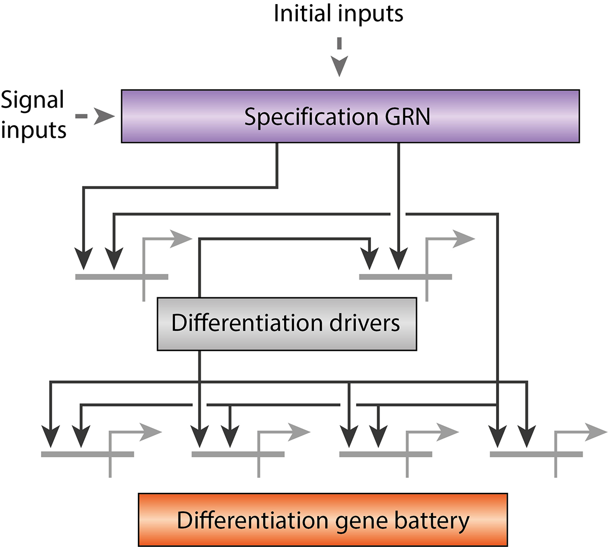
Plasticity and unpredictability

Development is not only characterised by constancy and predictability, but there is also plasticity and unpredictability. The chemistry of life is characterised by molecular fluctuations and stochastic events in cells that seem to contradict deterministic explanations of development. The examination of the complicated hierarchy of buffering in cells and organisms to maintain constancy, e.g. through GRN and other mechanisms, is a fascinating challenge for current and future research.

The phenomenon of phenotypic plasticity, i.e. the generation of alternative phenotypes from the same genome, shows that not every single developmental trait is fully determined by particular genes. The limited effect of the environment on phenotypes was proposed already in the early 20th century by the Danish botanist Wilhelm Johannsen who equated the genotype with the notion of reaction norm, which referred to the range of potential – reversible – phenotypic variations in different environments. An intriguing example is the transition between solitarious and gregarious locusts elicited by mechanosensory input (Fig. 3).

Throughout the history of modern biology, the ideas of genetic causality and biological specificity have been rejected or marginalised in various fields. Around 100 years ago, the movement of biocolloidy, focusing on unspecific physical mechanisms replaced the search for relations of specific structures and functions by theories related to surface actions, electric charges and adsorption. All biochemically relevant substances of the cell such as proteins, enzymes and nucleic acids were regarded as biologically active colloidal aggregates of undetermined composition. The success of macromolecular chemistry and, subsequently, molecular biology, brought forward approaches that were able to causally explain the phenomena of biological specificity, rendering biocolloidy obsolete.

Questioning genetic causality

More recently, some approaches of epigenetics try to call into question genetic causality by claiming that small, unspecific molecules such as methyl groups are able to regulate gene expression. Social scientists and some biologists believe that these epigenetic marks are environmentally caused and can be inherited over many generations, thus marginalising the causal role of the genome for development. However, these approaches ignore established scientific facts in genetics and cell biology, according to which gene regulation is brought about by specific regulatory proteins. Because the enzymes that transfer epigenetic marks to DNA or histones lack DNA-sequence specificity, they require sequence specific factors such as transcription factors to guide their activity on the genome. Thus, the factors that are involved in gene regulation are hierarchically organised.

Likewise, current attempts to explain animal development by non-hierarchical, multilevel, multifactorial mechanisms, deny the relevance or even existence of causal relationships between specific regulatory factors. They reject the explanatory power of hierarchical GRN on the grounds that transcription factors contain intrinsically disordered (ID) protein regions that render them unsuitable for regulatory purposes. However, it has been shown that these ID-regions occur predominantly in domains that are used e.g. for recruiting co-factors, and less in the DNA-binding domain. The fact that ID regions contribute to the instability of transcription factors is an important pre-requisite for their suitability for regulatory functions.

Non-hierarchical, multilevel, multifactorial network models may explain phenomena of plasticity. But they do not convincingly explain how:

Development can result in a functioning organisation,
The development of individuals of a species always results in the same body plan, largely independently of the environment,
How species can remain constant in different environments over long periods of time.

Historians and philosophers of science cannot predict scientific developments, as was formulated by biochemist and Nobel Laureate Otto Meyerhof some 90 years ago: “But one will only expect from scientific philosophy the consistent order of the system of scientific theories and no prediction of their contents.” However, historians and philosophers of science not only highlight the intellectual history of currently important concepts. They can also shed light on errors of reasoning and scientific dead ends, often due to neglect of basic biological principles that have been developed and revised since the late 19th century.

References:

Davidson, E.H. (2006). The Regulatory Genome. Gene Regulatory Networks in Development and Evolution. Burlington: Academic Press.

Gibson, G. (2002). Developmental Evolution: Getting Robust over Robustness. Current Biology 12, 347-349.

Deichmann, U. (2007). “Molecular” versus “Colloidal”: Controversies in Biology and Biochemistry, 1900–1940, Bulletin for the History of Chemistry 32, 105-118.

Deichmann, U. (2017). Hierarchy, Determinism, and Specificity in Theories of Development and Evolution. History and Philosophy of the Life Sciences 39 (4), 33. doi: 10.1007/s40656-017-0160-3

Deichmann, U. (2020). The Social Construction of the Social Epigenome and the Larger Biological Context. Epigenetics & Chromatin 13, 37. https://doi.org/10.1186/s13072-020-00360-w

Please note: This is a commercial profile

Contributor Details

Editor's Recommended Articles

Scientists witness the birth of early galaxies with James Webb Space Telescope

Amazing spike glowing lucky star and Milky Way Galaxy background - stock image

Investigating collapsing stars that mysteriously vanish

This artist concept shows a NASA-developed small-core jet engine installed in General Electric Aerospace’s CFM RISE jet engine design. The more fuel-efficient small core powers a large open turbofan, which also helps increase efficiency. The effort is part of NASA’s Sustainable Flight National Partnership to help inform the next generation of ultra-efficient airliners.

NASA collaborates with industry to design sustainable jet engine core

AI reveals differences in male and female brain structures

Quantum Computing - Quantum Supremacy - Supercomputers and Supercomputing - Innovation in Information and Computer Science - Conceptual Illustration on Technology Background

Supercomputing: UK boosts research access with EuroHPC £770 million membership

50000 Quaoar, dwarf planet, orbiting near Pluto planet. 3d render

Astrophysicist discovers fiery exoplanet with NASA’s TESS

Transfer RNA as a written molecular history of the life transition...

A very long oil train passing through a railyard in Havre, Montana, transporting fossil fuel from the oil fields of Williston, North Dakota. High resolution color photograph with copy space for your message. Horizontal composition.

Train derailment in East Palestine, Ohio: The toxic risks of transporting...

Thermodynamics of hadronization: The rotating lepton model explains key CERN experiments

Follow open access government, latest publication.

Open Access Government April 2024

Terms & Conditions
Privacy Policy
GDPR Privacy Policy
Marketing Info Pack
Fee Schedule

Explaining the Constancy of Species: Linneaus, Buffon, and Leibniz

February 15, 2014

Eric Voegelin

The Collected Works of Eric Voegelin

The transition from the transcendent to the immanent view can be traced in each aspect of the life problem . . . . We now turn to the transformation of the theory that is to explain the species characteristics of a life-form and their constancy through the generations.

The pure typical case of a transcendent explanation is Linnaeus’ theory, according to which God created at the beginning of the world the various animal species and endowed the individuals of each species with the ability to bring forth their own kind; in fact, the species was the quintessence of the individuals who have descended from each other through procreation; in theory the species was coined by God’s creative hand. When fixity of the species was understood in this way, there was hardly any reason to look for the inner causes of the individual’s character; the reference to God as the transcendent creator of the world in its thusness was sufficient.

Of all the theoreticians of biology of his day, Linnaeus was most deeply immersed in the Christian worldview. Linnaeus believed that the world actually had a definite beginning; there was a day and an hour when the world, in the organization of its existence, emerged from the chaos through God’s creating hand. When this belief died, the teaching of the species and its duration became questionable, leading to those transformations in the theory with which we must now concern ourselves.

When the world was no longer believed to be the creation of a higher being, the act of creation was no longer the real starting point in time of the world and its many species. The “world” was no longer a finite event that was on some level actually delimited in time by a transcendent being. And while the similarity of individuals had been understood as caused by a similar pressure of the divine hand, the theory of the fixity of the species was now also shaken. The succession of generations no longer had a finite beginning in the creation or an origin of its specific laws; instead, the succession could be traced from any individual back into infinity without this regression coming up against a point of origin for the law of the species.

The result was a peculiar, undecided state. The concept of creation was replaced by the idea of infinity. Preformist theory, which envisioned the germs of all individuals contained in the first progenitors of each species–for example, the human ones in the body of Eve–had to change, and replace this real definite beginning with the series of infinite encapsulations.

Now if the image of the created finite succession of generations is supplanted by the idea of an infinite succession without any real beginning, the idea that the law of this succession was created transcendentally at the beginning of the succession of generations becomes meaningless, and speculation forces us moreover to the formulation of that law in such a way that the law of the species can be directly discerned in each individual of the species.

A shift of the cause of the fixity of the species to infinitely distant specimens became pointless because according to the law of the infinite succession it must be assumed that each individual was descended from a predecessor. This led to the speculative leap to the lawfulness of the species as a real cause [ Realgrund ] that is at work in all individuals of a species, thus necessarily also in the one currently under observation, without having to be traced back to preceding ones.

This finitization of the law of the species in turn invalidates the idea of infinity that, for one speculative moment, served as the explanatory cause of the species–that is, for the moment when the act of creation had ceased to be the starting point of the succession of generations and it was still believed, in accord with the rationalistic encapsulation theory, that the regression to the preceding individual could explain the one descended from it. This open, undecided moment came to an end with the abolition of the idea of infinity and with the adaptation of the concept of law to the finite style of the new concept of the organism . . . .

Buffon Dissolves the Problem of Infinity

In his four propositions Linnaeus presented the species as created all at once and then subdivided into the generations of its individuals; the how of this process of individuation did not seem open to question. The succession became a problem only when biological inquiry starts with the individual and finds its attempt to explain the individual caught up in the infinite regress of encapsulations of preformed germs without coming any closer to an understanding of the concrete individual in its self-contained existence.

In this succession, in the continuous renewal and duration of the species, lies the mystery of nature, as Buffon argues when he attempts to fathom the nature of these succeeding generations and to elucidate the underlying problem. The ability to produce offspring of one’s kind, this curious lasting, apparently eternal unity–this to Buffon was the unfathomable mystery. The permanence of the species, which Linnaeus held to be the indisputable, God-created unitas of the series of individuals, becomes a problem for Buffon, who wants to understand the individual in its organic unity as a totality and as a totality of a specific kind.

He held those creatures to be individuals of a species who perpetuate themselves through copulation and thus preserve the image of the species. Individuals who do not produce offspring of their kind when they copulate must be regarded as belonging to different species. Thus, the chain of successive individual existences of the same species constitutes l’existence réelle de l’espèce. The infinite succession of generations with the same species characteristics is thus identical with the species itself, and Buffon then has to wonder whether seeing the individual as a part of this succession contributes anything to an understanding of the individual as a selfcontained being. Buffon answers in the negative and justifies his position by dissolving the problem of infinity.

He presents an excellent explanation of the genesis of the concept of infinity through the gradual addition of finite steps and demonstrates that the concept of infinity becomes meaningless if we keep in mind that the infinite regression is made up of finite steps. The infinite is nothing more than the finite realm with the boundaries removed; these boundaries are by nature a matter of quantity. As a result the infinite has become an intrinsically absurd concept. There is no actual infinite–that is, something infinite cannot be a subject of finite thinking. Regarding the problem of species this means that the inquiry has to start with the self-contained unity of the individual, which is determined by its species.

Several such unities of the same species form a finite series or succession, and from here theory (at any rate the preformation theory) makes the leap of attempting to explain the nature of the species on the basis of the infinite succession. However, according to Buffon, this infinity does not really exist; it is no existence actuelle but an abstraction. By nature extension is finite; to assume an actually infinite extension is a contradiction in terms. Those who nevertheless make such an assumption, according to Buffon, have to confine themselves to saying that the infini de successions et de multiplications is nothing more than an extension with an indefinite upper limit–not an infini but an indéfini.

Pointing out the infinite divisibility of matter also does not hold good; rather this argument must be countered with the point that the same illusions connected with the infinite divisibility are also associated with all other kinds of mathematical infinity: these infinities do not exist in actual fact but are merely intellectual abstractions. Therefore, dissolving the species into an infinite regression is not a sufficient answer to the question of how we are to understand the nature and reproduction of life-forms.

We can understand Buffon’s reasoning only if we assume a complete breakdown of the idea Linnaeus had still considered valid, namely, that of a finite, self-contained world created by God. In this self-contained worldview, the creation of the species unit by God is a completely adequate explanation of the species characteristics of the individual.

It is only when the rampartlike boundaries of this world are breached and the succession of generations extends into infinity that the problem of actual infinity becomes discernible in ameaningful way. It is only when the dogmatic framework breaks down and the empirical stance attempts to understand the isolated individual in its particularity that the problem Buffon presents arises.

Leibniz and Speculation on the Infinite

At the end of the chapter of Buffon’s Histoire naturelle (p.250) that contains the investigations of the problem of infinite we find the date February 6, 1746; the volume was published in 1750. For further details concerning his ideas, Buffon refers the reader to the foreword of his translation of Newton (not available to me), which appeared in 1740, and thus to the larger mathematical context of the problems associated with the analysis of infinity in his time.

The most significant and most concise fundamental formulations of the problem are found in some letters from Leibniz to Bernoulli (published in 1745). For our purposes the letter of July 29, 1698,is especially important because it contains a statement referring to the problem of preformation. There Leibniz speaks about the division of matter, arguing that no indivisible elements or smallest particles can ever be arrived at, only ever smaller ones that can be split into yet smaller ones.

By the same token, increasing a dimension will never lead to the largest one or to infinitely large ones or to ones whose dimensions cannot be increased further. Applying these principles to the problem of preformation, Leibniz concedes that the germs may be encapsulated but denies that it is possible to arrive at an infinitely small one, much less at an ultimate one.

The regression of encapsulation is thus extended into infinity, and the act of creation loses its significance as an absolute beginning. Another passage in a letter of August, 1698, shows even more clearly that in the infinite regression for each member we must necessarily envision another one, and thus the concept of an absolute infinity is a contradiction in terms. The passage is formulated with particular felicity because it distinctly shows the connection between the problem of the infinitely large with that of the infinitely small; from the vantage point of empirical finite facts, speculation on infinity leads to meaninglessness in both directions. 1

“Since I have denied arriving at minimal portions, it was easy to judge that I was not speaking of our divisions, but also about those actually occurring in nature. Therefore, although I certainly hold that any part of matter whatsoever is actually subdivided again, still I do not think it therefore follows from this that there exists an infinitely small portion of matter, and still less do I concede that it follows that there exists any altogether minimal portion. If anyone wishes to pursue the consequence formally, he will sense the difficulty.”

“But you will inquire: If nothing infinitely small exists, then single parts are finite (I concede); if singular parts are finite,therefore all taken together at once constitute an infinite magnitude. I do not concede this conclusion. I would concede, if there existed some finitude which would be smaller than all others or certainly not greater than any other; for then I confess that on such assumptions, by as many as any given number you like there arises a quantity as large as you like. But it holds true that by any part you like another smaller finite magnitude exists.”

The problem of the given fact of an actual infinite again plays an important role in the history of modern mathematics, especially in the construction of Cantor’s set theory and theory of transfinite cardinal numbers, sets of sets, and so forth. This development in mathematics is essentially based on the same false reasoning Leibniz discussed in his letters to Bernoulli and Buffon addressed in the context of his criticism of the theory of preformation. Lately Felix Kaufmann has tried in his works to resolve this false reasoning of set theory and the mathematical theory based on it. His argumentation is essentially the same as Buffon’s, cited earlier in the text.

I quote from Kaufmann’s book, Das Unendliche in der Mathematik und seine Ausschaltung (Vienna, 1930), 147:

“We have established that the natural numbers are logical abstracts of the counting process and that the concept of the ‘number series’ includes an ‘idealization’ in addition to this abstraction. It consists of the presupposition of the nonexistence of a fixed upper limit, so that ‘number series’ comes to mean the abstraction of an infinite counting process.”

He points out that we must avoid the error “of seeing a self-contained totality of natural numbers in the number series”(148). We must start with the counting process and determine its logical structure; the series of natural numbers must be defined by the law of their formation and not conversely the general form of the process by its product, assumed to be real.

In his “Bemerkungen zum Grundlagenstreit in Logik und Mathematik” ( Erkenntnis , II, 1931) Kaufmann summarized the problem most concisely in the sentence (285): “The circularity (namely, of the concept of the infinite series of natural numbers) lies in the fact that in general where no final limit exists for the number of the function values, the value trend [ Wertverlauf ] of a function can be defined only as a general form, and therefore it is not possible to define this general form by the value trend.”

This excerpt is from The History of the Race Idea: From Ray to Carus (Collected Works of Eric Voegelin 3) (Columbia, MO: University of Missouri Press, 1998)

Eric Voegelin (1901-85) was a German-born American Political Philosopher. He was born in Cologne and educated in Political Science at the University of Vienna, at which he became Associate Professor of Political Science. In 1938 he and his wife fled from the Nazi forces which had entered Vienna and emigrated to the United States, where they became citizens in 1944. He spent most of his academic career at the University of Notre Dame, Louisiana State University, the University of Munich and the Hoover Institution of Stanford University. More information about him can be found under the Eric Voegelin tab on this website.

Subscribe to VoegelinView via Email

Stay informed with the best in arts and humanities criticism, political analysis, reviews, and poetry. Just enter your email to receive every new publication delivered to your inbox.

Email Address

Help | Advanced Search

Quantitative Biology > Neurons and Cognition

Title: an investigation of conformal isometry hypothesis for grid cells.

Abstract: This paper investigates the conformal isometry hypothesis as a potential explanation for the emergence of hexagonal periodic patterns in the response maps of grid cells. The hypothesis posits that the activities of the population of grid cells form a high-dimensional vector in the neural space, representing the agent's self-position in 2D physical space. As the agent moves in the 2D physical space, the vector rotates in a 2D manifold in the neural space, driven by a recurrent neural network. The conformal isometry hypothesis proposes that this 2D manifold in the neural space is a conformally isometric embedding of the 2D physical space, in the sense that local displacements of the vector in neural space are proportional to local displacements of the agent in the physical space. Thus the 2D manifold forms an internal map of the 2D physical space, equipped with an internal metric. In this paper, we conduct numerical experiments to show that this hypothesis underlies the hexagon periodic patterns of grid cells. We also conduct theoretical analysis to further support this hypothesis. In addition, we propose a conformal modulation of the input velocity of the agent so that the recurrent neural network of grid cells satisfies the conformal isometry hypothesis automatically. To summarize, our work provides numerical and theoretical evidences for the conformal isometry hypothesis for grid cells and may serve as a foundation for further development of normative models of grid cells and beyond.

Submission history

Access paper:.

HTML (experimental)
Other Formats

References & Citations

Google Scholar
Semantic Scholar

BibTeX formatted citation

Bibliographic and Citation Tools

Code, data and media associated with this article, recommenders and search tools.

Institution

arXivLabs: experimental projects with community collaborators

arXivLabs is a framework that allows collaborators to develop and share new arXiv features directly on our website.

Both individuals and organizations that work with arXivLabs have embraced and accepted our values of openness, community, excellence, and user data privacy. arXiv is committed to these values and only works with partners that adhere to them.

Have an idea for a project that will add value for arXiv's community? Learn more about arXivLabs .

Short Report
Open access
Published: 23 May 2024

Identification of the RSX interactome in a marsupial shows functional coherence with the Xist interactome during X inactivation

Kim L. McIntyre 1 na1 ,
Shafagh A. Waters 2 na1 ,
Ling Zhong 3 ,
Gene Hart-Smith 4 ,
Mark Raftery 3 ,
Zahra A. Chew 5 ,
Hardip R. Patel 5 ,
Jennifer A. Marshall Graves 6 &
Paul D. Waters ORCID: orcid.org/0000-0002-4689-8747 1

Genome Biology volume 25 , Article number: 134 ( 2024 ) Cite this article

313 Accesses

8 Altmetric

Metrics details

The marsupial specific RSX lncRNA is the functional analogue of the eutherian specific XIST , which coordinates X chromosome inactivation. We characterized the RSX interactome in a marsupial representative (the opossum Monodelphis domestica ), identifying 135 proteins, of which 54 had orthologues in the XIST interactome. Both interactomes were enriched for biological pathways related to RNA processing, regulation of translation, and epigenetic transcriptional silencing. This represents a remarkable example showcasing the functional coherence of independently evolved lncRNAs in distantly related mammalian lineages.

The sex chromosomes of therian mammals (marsupials and eutherians) share a common ancestry [ 1 ], having evolved from a pair of autosomes [ 2 ] after the divergence of therian and monotreme mammals approximately 187 mya [ 3 ]. X chromosome inactivation (XCI) occurs in both groups of mammals, implying an ancient origin. However, XCI in eutherians and marsupials involve molecular mechanisms that are remarkably different.

XCI in therian mammals silences transcription of one of the two X chromosomes in female somatic cells [ 4 ]. It is established in the early embryo and maintained through subsequent cell divisions and serves as an important model for epigenetic silencing due to its unparalleled scale and stability. Long-noncoding RNAs (lncRNAs) have emerged as common regulators in therian XCI. Eutherian XCI is mediated by a lncRNA called XIST [ 5 ]. Its mouse orthologue, Xist [ 6 ], shares ~ 67% sequence conservation with human XIST. This includes a series of tandem repeats (A to F), of which only repeat A is well conserved across all eutheria [ 7 ].

The protein interactome of Xist has been investigated in mouse cell lines using techniques involving chromatin isolation by RNA precipitation with mass spectrometry (ChIRP-MS) and its variations [ 8 , 9 , 10 , 11 , 12 ]. These investigations have identified 494 proteins in total, with only 6 proteins (Hnrnpm, Hnrnpu, Myef2, Raly, RBM15, Spen) common to all studies [ 8 , 9 , 10 , 12 ]. An alternative technique, RNA immunoprecipitation (RIP) combined with deep sequencing, identified epigenetic regulators in the human XIST interactome that were not identified in the mouse studies: EZH2 and SUZ12, subunits of polycomb repressive complex 2 (PRC2), and CHD4, a subunit of the NuRD histone deacetylase complex [ 13 , 14 ].

Marsupials lack an XIST gene; instead, ancient protein-coding genes have been retained at the loci homologous to those from which XIST and neighbouring genes evolved in eutherians [ 15 , 16 , 17 ]. In marsupials, XCI is mediated by a lncRNA called RSX [ 18 ] that is derived from a non-homologous and physically distinct region of the X chromosome. RSX is 27 kb in Monodelphis domestica (grey short-tailed opossum) [ 18 ] and 30 kb in koala ( Phascolarctus cinereus ) [ 19 ], longer than the 15 kb mouse Xist [ 6 ] and the 17 kb human XIST [ 20 ]. Although lacking linear sequence homology, a k-mer analysis classified two major groupings of repeat domains that are shared between Xist and RSX ( RSX repeat 1 with Xist repeats B, C and XIST repeat D, and RSX repeats 2, 3 and 4 with Xist repeats A and E). Each of these domains is enriched for specific protein binding motifs [ 21 ]. Therefore, although RSX and Xist share no sequence homology they could be functional analogues.

Xist and RSX are both nuclear transcripts that are spliced, capped and polyadenylated in the manner of mRNAs, and are expressed only in female somatic cells, exclusively from the inactive X chromosome. In both cases, the clustered transcripts can be visualised using RNA fluorescence in-situ hybridisation (RNA FISH) as a distinctive cloud-like signal accumulated on the inactive X chromosome [ 18 , 20 ]. Induction of RSX expression from an autosomal transgene in mouse silences transcription in cis [ 18 ]. This indicates a silencing capacity similar to that of Xist [ 22 ], although marsupial XCI is ‘leakier’ or more incomplete than the XIST -driven process in eutherians [ 23 ], perhaps due to the evolution of two different lncRNAs in different ancestral genomic contexts.

Here, we investigate the protein interactome of RSX in a marsupial, Monodelphis , and compare it with the Xist protein interactome. We consider the molecular mechanisms underlying the convergent evolution of XCI in therian mammals to enhance understanding of the evolution of the adaptations for balancing gene expression between the sexes. Our findings show that RSX interactors significantly overlap with Xist interactors, falling within the same protein–protein association network related to RNA splicing and processing, translation regulation and ribosome biogenesis, and epigenetic transcriptional silencing. This highlights the remarkable functional coherence of these non-homologous and independently evolved lncRNAs. We identified overlap between the Xist and RSX protein interactomes, both of which are enriched for functions associated with post-transcriptional regulation of gene expression. Post-transcriptional regulation has been shown to contribute to the balancing of expression of X-borne genes between the sexes in eutherians [ 24 , 25 , 26 , 27 ], although the underlying mechanisms are unknown.

Identification and validation of RSX interactors and comparison with Xist interactome

To investigate the protein interactome of RSX we used ChIRP-MS to capture proteins associated with RSX using six biotinylated oligonucleotides complementary to different RSX regions (Additional file 1 ). Cell lysates were prepared from female Monodelphis fibroblast cells that were either UV crosslinked, formaldehyde crosslinked, or uncrosslinked. We identified 131 proteins that were associated with RSX using alternate criteria of presence/absence and greater than two-fold enrichment versus a control, either absence of oligonucleotides or scrambled oligonucleotides (Fig. 1 A, Additional file 2 ).

RSX and Xist interactomes share common orthologous proteins and protein–protein association networks with distinctive functional enrichments. A Overview of ChIRP-MS workflow. * Two proteins were identified by a single pulldown from a UV crosslinked sample. ** includes 4 additional proteins identified using RIP-qPCR. Graphic created using BioRender.com. B Protein–protein interactions of the RSX and Xist interactomes based on experimentally determined interactions, co-expression, and curated database annotations for human orthologs (STRING database v11.5) [ 28 ]. Each node represents an interactome protein, each edge represents an annotated protein–protein interaction of minimum confidence 0.4. Interaction networks were visualised using Cytoscape (v3.8.2) [ 29 ], omitting proteins with no annotated interactions. Nodes were clustered based on connectivity (number and weight of edges) using the GLay Cytoscape plugin [ 30 ] with default settings. Intercluster edges to minor clusters (4–10) omitted for clarity. # denotes mean intracluster node degree (21). C Key functional and structural enrichments of each major protein interaction cluster. GSEA was conducted using gProfiler2 [ 31 ] with multiple testing correction based on false discovery rate. D Enrichment of RSX (fold change relative to Igg controls) by immunoprecipitation of protein targets from female Monodelphis fibroblast cell lysates, followed by quantitative PCR using RSX -specific primers. Enrichment (30-fold) was also detected for HNRNPK, as previously published [ 21 ]

We validated two RSX interactors using RNA immunoprecipitation (RIP) followed by quantitative PCR (qPCR). The RIP targets were chosen for their potential role in XCI. In eutherian models, SUZ12/EZH2 (core components of PRC2), HDAC2, HNRNPK and CTCF have roles in eutherian XCI. MBD2 + 3, MBD4, and MECP2 bind methylated DNA and are involved in chromatin remodelling and gene regulation. The histone marks H3K9me3 and H3K27me3 are known to accumulate on the inactive X in marsupials [ 32 , 33 ]. PCAF is an acetyltransferase, so served as a negative control (Fig. 1 D). Target proteins were immunoprecipitated from female Monodelphis fibroblast cell lysates, followed by qPCR using RSX -specific primers [ 21 ]. Enrichment of RSX (relative to IgG controls) of greater than tenfold was detected for seven targets. These included HNRNPK [ 21 ] and SFPQ, which were identified by the ChIRP-MS. The RIP-qPCR also identified four additional RSX interactors not detected by ChIRP-MS: EZH2 (PRC2 catalytic subunit), HDAC2 (a histone deacetylase), MBD4 (a methyl-CpG binding domain protein), and MECP2 (a methyl-CpG-binding protein).

These proteins were included in the RSX interactome, bringing the total to 135 proteins. We considered whether proteins of the RSX interactome had orthologues in the Xist interactome. Of the 135 RSX -interactors, 81 did not have orthologues in the Xist interactome, so were specific to the RSX interactome. The remaining 54 RSX -interactors had orthologues that were identified in the Xist interactome (which comprises 497 proteins in total). Therefore, we identified a substantial cohort of proteins that interact with both RSX and Xist , despite the lack of homology in the primary sequence of these two lncRNAs. We also considered the extent to which the two interactomes might include different proteins from common functional pathways, potentially providing insights into how therian XCI evolved to be mediated by different lncRNAs in marsupials and eutherians.

Network analysis of the RSX and Xist interactomes reveals functional similarities

Gene set enrichment analysis (GSEA) [ 34 ] of each of the RSX and Xist interactomes identified that over 90% of the 136 ontology terms enriched for the RSX interactome were also enriched for the Xist interactome ( p < 1 × 10 −3 ) (Additional file 3 : Tab 5), suggesting functional similarities between the two interactomes.

We queried the protein–protein interactions within the combined RSX and Xist interactomes using the STRING database (v11.5), with experimental findings, co-expression data, and evidence from curated databases as interaction sources [ 28 ]. Of the 578 proteins in the combined interactomes, 516 proteins had at least one interaction (confidence score > 0.4) and formed a network with 8721 edges (a mean of 15.1 edges per node). This was significantly higher than the 3633 edges expected for a random set of 578 proteins selected from the same proteome ( p < 1 × 10 −16 ). Clustering of the interaction network partitioned it into three larger clusters and five small clusters (Fig. 1 B, Additional file 4 : Tab 1). The key functional enrichments of each of the three major clusters were determined using GSEA. The three large clusters were individually enriched for functions including mRNA binding, translation (and regulation of translation), and nitrogen compound catabolic process (Fig. 1 C, Additional file 3 : Tab 4). In addition to these common terms, the clusters had distinctive functional enrichments, including ribosomal biogenesis in cluster 1, RNA splicing and processing in cluster 2, and chromatin modification and epigenetic silencing in cluster 3 (Fig. 1 C, Additional file 3 : Tabs 1–3, with Column E in each case listing the interactome proteins underlying each enriched ontology term, Additional file 5 : Fig. S1).

Clustering and enrichment analyses were also conducted on the RSX and Xist interactomes separately using the same approach. Each interactome had four major clusters, with GSEA enrichments reflecting those of the combined interactome analysis, subject to division of cluster 2 in the RSX interactome, and division of cluster 1 in the Xist interactome (Additional file 5 : Fig. S2).

RSX -specific interactome proteins were of interest in unravelling the differences between eutherian and marsupial XCI. GSEA of the 81 RSX -specific proteins identified enrichments for spliceosomal complexes, ribosomal subunits, cytosolic translation, nucleosome binding and chromatin organisation (Additional file 3 : Tab 6) in proportions similar to those of the overall RSX interactome, other than perhaps for nucleosome binding which predominantly involves RSX -specific proteins. Apart from this, RSX -specific proteins did not appear to have gross unique function compared to the full RSX interactome.

Collectively, the clustering and GSEA enrichment analyses revealed an overlap between the RSX and Xist interactomes. This encompassed common proteins and also interactions with different proteins in common molecular pathways, providing insights into the functions modulated by RSX and Xist.

Functional analysis of HNRNPK in Monodelphis XCI

We focused on the functional role of HNRNPK, which was identified in our RSX interactome and is also an Xist -interacting protein. HNRNPK is important in recruiting polycomb repressive complex 1 (PRC1), a significant part of the epigenetic silencing machinery, during eutherian XCI [ 11 , 35 ]. In the combined RSX/Xist interactome network it was in cluster 2, which was enriched for functions in RNA splicing and processing (Fig. 1 B). We depleted HNRNPK expression in a female Monodelphis fibroblast cell line using RNA interference (RNAi), adapting eutherian-based construct design and delivery for our non-traditional model organism. We assessed the effect on XCI using RNA FISH, which allowed us to determine the transcriptional status of MSN, an X-borne gene that is usually silenced on the inactive X chromosome, which should have monoallelic expression. In control nuclei (transfected with an empty RNAi vector) biallelic expression of MSN (indicating transcription from both X chromosomes) was detected in only 18% of cells ( n = 286; Additional file 5 : Figs. S3 and S4). Knockdown efficiency was assayed by measuring transcript abundance using RT-qPCR. The knockdown effect on protein abundance may differ due to variations in post-transcriptional processing.

Following HNRNPK knockdown (by ~ 24–35%) biallelic expression of MSN increased from 18% in control cells to 39% in cells with depleted HNRNPK expression ( n = 159; p = 1.0 × 10 −11 chi-squared test goodness of fit test) (Additional file 5 : Figs. S3 and S4). Increased biallelic expression of MSN signified reactivation of transcription from the silenced allele on the inactive X chromosome. This outcome was observed across two independent experiments, and provides evidence that HNRNPK plays a role in maintenance of transcriptional silencing on the inactive X chromosome in Monodelphis .

Functional analysis of CKAP4 in Monodelphis XCI

CKAP4 has not been identified as an Xist interactor, and has no predicted interactions with any protein in either the Xist or RSX interactomes (Additional file 4 : Tab 3). In the RSX interactome, CKAP4 was unexpectedly the protein with the highest fold-change (20 ×) enrichment relative to controls in the native (uncrosslinked) ChIRP-MS (Additional file 2 : Tab 2). Therefore, we used RNAi to suppress CKAP4 in female Monodelphis fibroblasts by ~ 53–55%. We observed an increase in biallelic expression of MSN from 18 to 26% ( n = 165; p = 8.7 × 10 −3 Chi Squared Test Goodness of Fit Test). This suggests that CKAP4 plays a role in maintenance of Monodelphis XCI.

Interestingly, despite the absence of CKAP4 from the GSEA analysis of the combined interactome network, the rough endoplasmic reticulum (where CKAP4 is usually localised) was significantly enriched in cluster 1 ( p = 1.1 × 10 −6 ), along with three other associated terms ( p < 9.8 × 10 −4 ) (Additional file 3 : Tab 1). This finding aligns with the functional enrichment of ribosomal and translation-associated machinery observed in the same cluster.

The role of CKAP4 in marsupial XCI prompted a comparative analysis of its protein sequences across a broad phylogenetic spectrum, including eutherians (mouse, human, and hyrax — an afrotherian), monotremes (platypus and echidna), and eight marsupial species. This comparative sequence analysis (Fig. 2 A), unveiled a large expansion of a glutamine (Q)-rich repeat at the N-terminus in the Monodelphis CKAP4, which contrasted eutherians, monotremes and most other marsupials.

CKAP4 has a glutamine-rich repeat expansion in monodelphis. RSX and Xist interactomes are enriched for proteins with IDRs. A Protein sequence alignments of representative mammalian CKAP4. An expansion of a glutamine (Q) rich repeat was observed at the N-terminus in Monodelphis and yellow footed antechinus. Inset shows a subregion of the repeat expansion. B AlphaFold predicted structure of Monodelphis CKAP4, with the Q rich repeats highlighted in black. C Alignment of predicted CKAP4 structures for human (blue), mouse (red), hyrax (orange) and Monodelphis (green and black). Sequence independent RMSD values (for all atoms with outlier rejection) of Monodelphis CKAP4 to the eutherian orthologues were 24.5 Å (human), 24.5 Å (mouse), and 13.7 Å (hyrax). D Median protein IDR scores for the RSX and Xist interactomes represented as violin plots (depicting density distribution) overlayed with boxplots depicting the median for all proteins of the RSX and Xist interactomes (mouse orthologs), and randomly sampled proteins of a subset of the mouse proteome comprising only proteins within the gene ontology terms enriched in clusters 1, 2 and 3 (20 × sets of 200 proteins). Statistical significance assessed using Dunn’s test (with Holm adjustment) for pairwise comparisons, following Kruskal–Wallis test

We employed AlphaFold to predict the tertiary structures of CKAP4 in Monodelphis alongside three representative eutherian species: human, mouse, and hyrax (Fig. 2 B and C). The structural predictions highlight a distinctive helical conformation within the Poly Q-rich N-terminus of Monodelphis CKAP4 (2B). Such structural motifs are known for their stability and propensity to engage in functional interactions with RNA and proteins [ 36 ], and provides a molecular mechanism by which Monodelphis CKAP4 could interact with RSX .

Enrichment of proteins with intrinsically disordered regions (IDRs) in the RSX interactome

Recent studies have revealed that the Xist compartment is founded on an assembly of dynamic RNP complexes comprising Xist RNA in association with the intrinsically disordered regions (IDRs) of Xist -interacting proteins, such as SPEN, PTBP1, MATR3, CELF1, and CIZ1 [ 37 , 38 , 39 , 40 ]. Of these, only PTBP1 was identified in the RSX interactome, so we considered whether other proteins with IDRs might also be present in the RSX interactome.

We assessed the proportion of proteins enriched for IDRs in each interactome with IUPred2A [ 41 ], which calculates a disorder score for each residue using amino acid composition and energy estimation. Disorder scores above 0.5 (range 0 to 1) correspond to disordered residues. We calculated the IDR score for each protein as the median disorder score of its residues. We found that RSX interactome proteins had higher median IDR scores than the Xist interactome proteins ( p = 2.5 × 10 −9 ). Both interactomes had higher median IDR scores ( p = 1.4 × 10 −27 for RSX and p = 2.7 × 10 −16 for Xist ) than a randomly sampled group of 200 proteins from a subset of the reference proteome (Fig. 2 D). The background proteome subset comprised all proteins within the ontology terms (Additional file 3 , Tabs 1–3, column A) enriched ( p < 1 × 10 −3 ) in one or more of the combined interactome clusters 1, 2 and 3. Proteins common to both the RSX and Xist interactomes had higher median IDR scores than proteins that interact exclusively with either RSX or Xist ( p = 2.5 × 10 −2 cf RSX , p = 1.4 × 10 −10 cf Xist ) (Additional file 5 : Fig. S5A).

IDRs have important roles in supporting protein–protein interactions, protein-RNA interactions, and the formation of phase-separated condensates that form nuclear subcompartments [ 42 , 43 , 44 ]. Our finding suggests that an enrichment for proteins with IDRs may play a role in the formation of RSX -associated RNP complexes, aiding subcellular organisation, as has been identified for Xist -associated RNPs.

This research provides a novel insight into the complex protein interactions of RSX , a lncRNA in marsupials with a role similar to the eutherian Xist in epigenetically silencing the inactive X chromosome. We found that that the RSX interactome has functional enrichments analogous to Xist that underscore their functional similarities. We also showed that alleles on the inactive X chromosome were partially reactivated following the partial depletion of HNRNPK and CKAP4, two proteins in the RSX interactome, indicating a role for each in marsupial XCI maintenance.

Of note was the glutamine (Q)-rich repeat at the N-terminus of CKAP4. Poly-Q motifs play a pivotal role in modulating protein–protein interactions, often leading to the formation of aggregates with distinct biological consequences [ 36 ]. The structure of the Poly-Q rich repeat in Monodelphis CKAP4 suggest a novel change that might underpin its different function when compared to the eutherian counterpart. The helical conformation of Monodelphis CKAP4 N-terminus could enhance affinity for RNA and/or proteins, which could enable its binding with RSX . Interestingly, the Poly-Q motif expansion is not common to all marsupials, appearing to be specific to Monodelphis and a species of antechinus, suggesting linage specific adaptation.

LncRNAs provide an important organising mechanism in epigenetic regulation, including in the recruitment and sequestration of RNA splicing and processing factors. Many of these proteins are multifunctional, often with distinct nuclear and cytoplasmic functions. This interaction of lncRNAs with multifunctional proteins can provide an efficient mechanism by which lncRNAs can impact diverse molecular networks. Of the 54 proteins identified in common in the RSX and Xist interactomes, 43 form part of interactome network cluster 2, which features proteins involved in RNA splicing and processing.

The 54 proteins common to both interactomes were enriched for intrinsically disordered regions (IDRs), a characteristic identified in each interactome individually. These IDRs could potentially contribute to epigenetic silencing by facilitating protein–protein interactions, as proteins enriched in IDRs are characterised by their flexible and adaptable binding with multiple partners. This binding plasticity may contribute to the dynamic regulation of gene expression on the inactive X chromosome, potentially including alternate silencing and escape from silencing, depending on specific cellular contexts. Further, this plasticity might be important for the observed ‘leakiness’ of XCI observed in marsupials as partial or full expression from the inactive X chromosome [ 45 , 46 ].

Analysis of interactome network clusters 1 and 3 provided further insight into the mechanisms by which RSX and Xist might regulate gene expression. GSEA of each of these clusters indicated a functional coherence: despite a relatively small overlap in interactomes, they had different protein interactors involved in shared pathways. Cluster 1 was functionally enriched for ribosomal biogenesis, rRNA processing and regulation of translation. For RSX , this is consistent with the nucleolar association of the inactive X in marsupials. Cluster 3 contained proteins typically associated with XCI, including those involved in epigenetic regulation of transcriptional silencing, histone modifications and heterochromatin. These proteins include SPEN, which was identified in all of the Xist ChiRP-MS studies but was absent from the RSX interactome. SPEN is required for upregulation of Xist during XCI initiation [ 47 ], but becomes less important during the maintenance stage [ 48 ]. Therefore, it was not unexpected that SPEN was absent from the RSX interactome in our fibroblast model, which represents XCI maintenance.

Enrichment of functions associated with post-transcriptional regulation is a fascinating aspect of the Xist and RSX interactomes. Post-transcriptional regulation of X-borne gene expression has been identified in eutherians and Monodelphis by comparing gene expression in the transcriptome and translatome (based on ribosomal occupancy) [ 24 ]. Balancing of sex chromosome-borne gene expression between sexes in the proteome has also been identified in the more distantly related platypus ( Ornithorhynchus anatinus ) and chicken ( Gallus gallus ). This highlights the possibility of post-transcriptional regulation being an ancestral strategy for fine tuning the expression of sex chromosome genes in both sexes [ 49 ]. Our understanding of the evolution of the therian sex chromosomes suggests that silencing of X-borne genes would have evolved as the X and Y chromosomes diverged, perhaps initially involving other noncoding RNAs and only localised silencing before the Y chromosome was as degraded as it currently is. The emergence of independent chromosome wide regulation of XCI by XIST and RSX would then have coordinated presumably more efficient silencing, balancing the expression of X-borne genes between the sexes as degeneration of the Y chromosome progressed.

Conclusions

This work highlights a striking example of convergent evolution of lncRNA protein interactome evolution that achieves XCI in diverse mammalian clades. The independently evolved XIST and RSX recruit similar molecular pathways to repress the activity of almost an entire chromosome. These molecular pathways are associated with epigenetic transcriptional silencing, which typifies XCI, in addition to post-transcriptional regulation of gene expression, notably RNA splicing and processing, translation regulation and ribosome biogenesis. The functional coherence between the RSX and Xist interactomes, and the prevalence in both interactomes of proteins enriched for IDRs, adds a novel and critical dimension to our understanding of lncRNA mediated epigenetic regulation.

Cell culture

Female Monodelphis fibroblasts were cultured at 35 °C with 5% CO 2 in Dulbecco’s modified Eagle’s medium (DMEM), 10% v/v Newborn Calf Serum, 0–10% v/v AmnioMAX™-C100. Cells were passaged at 70–100% confluency using Trypsin–EDTA (0.25% w/v) (Thermo Fisher Scientific).

Cells were cultures on 15-cm plates to 70–80% confluence. Three plates (~ 6 µg total protein) were used for each pulldown. Cross-linking of samples occurred prior to cell harvest using either: (1) UV using Stratalinker UVP Crosslinker CL-1000 (200 mJ/cm 2 at 200 nm) on ice in 10 ml of phosphate buffered saline (PBS); or (2) 3% formaldehyde solution in PBS (30 min, RT) followed by quench in 0.125 M glycine for 5 min. ‘Native’ samples were not cross-linked. Cells were scraped from the plate into Eppendorf tubes and pelleted at 500 rcf for 5 min at 4 °C. Cell pellets were alternately flash-frozen and stored at – 80 °C, or proceeded directly. The cell pellet was resuspended (1 ml per plate of cells) in NP-40 buffer with Roche cOmplete™, EDTA-free Protease Inhibitor Cocktail (1 tablet per 7 ml of NP-40 buffer) and incubated for 15 min either: 1) at 4 °C on rotating platform; or) on ice, with vortexing for 5 s every 5 min. Cell lysates were sonicated using a Q700 sonicator (Qsonica) in a 4 °C water bath at amplitude 16 for 12 min pulsing 30 s on/off. Sonicated cell lysates were pelleted at 20,000 rcf for 5 min at 4 °C. Supernatant lysate was removed and assayed for total protein concentration using a Qubit™ fluorometer. Aliquots of 1.5 ml of supernatant (~ 3 µg total protein) were combined with 50 µl of prepared Dynabeads™ M-280 Streptavadin (beads). Beads were prepared in accordance with manufacturer’s guidelines with the following modifications: 100 µl of resuspended beads were used for each sample. After washing in 1 × Binding + Wash buffer (10 mM Tris–HCl (pH 7.5) 1 mM EDTA 2 M NaCl), beads were washed twice in Solution A (DEPC-treated 0.1 M NaOH DEPC-treated 0.05 M NaCl) followed by twice in Solution B (DEPC-treated 0.1 M NaCl), in each case vortexing for 5 s before magnetic capture for one min. Suspended beads were divided into 100 µl aliquots before final magnetic capture, followed by addition to each aliquot 200 µl of 2 × B + W buffer, 5 µl of 100 mM biotin-labelled oligonucleotide (omitted for control) and 195 µl of DNase-free H 2 O. Samples were incubated for 15 min at room temperature on slow rotating platform. Beads were magnetically captured for 3–5 min, before removal of clear supernatant. Beads were washed 3 times with a 1 × B + W buffer (200 µl) on rotation for 2 min with a one min magnetic capture. Beads were re-suspended in 100 µl of NP40 Buffer, before dividing between the two 1.5-ml aliquots of supernatant for each sample. Lysates were incubated with the pre-cleared beads on a rotating platform overnight at 4 °C. Beads were magnetically captured for one min at 4 °C, and supernatant removed. The beads for each sample were then washed with twice with 2 ml of NP40 Buffer (divided equally between the bead aliquots for the first wash before combining for the second wash), followed by twice for 15 min with 1 ml RIPA Buffer on rotating platform at 4 °C. After the final magnetic capture, the supernatant was removed. One hundred microliters of pre-warmed (65 °C) Elution Buffer (10 mM Tris–HCl, pH 6.0, 1 mM EDTA, 2.0M NaCl) was added to the supernatant before incubating for 20 at 65 °C with shaking. The supernatant was magnetically cleared of beads twice before assaying the protein concentration of the supernatant using a Qubit™ fluorometer, and submitting for LC/MS–MS. For validation, supernatant containing 20–60 μg of protein was dissolved in 1 × Laemmli Buffer (Bio-Rad), heated to 95 °C for 10 min to denature, and then size-separated on a 7.5% SDS-PAGE gel (Bio-Rad TGX) in 1 × Tris/Glycine/SDS (TGS) Buffer (Bio-Rad) at 160 V. Protein gels were washed in Milli-Q water three times for 5–10 min each before staining overnight in Commassie blue, washing in RO water three times and then excising protein bands.

Probe design

ChIRP-MS probes (Additional file 1 ) were designed using online tools [ 50 ]. Oligonucleotide probes were synthesised with 3′ Biotin-TEG, obtained from Integrated Data Technologies, Inc.

For each pull-down oligonucleotide probes were either pooled, or used individually. Probe 3 targeted the RSX Repeat 1. A probe with no homology to any sequence in the Monodelphis genome was used as an additional control to filter proteins identified in native (uncrosslinked) pull-downs.

Mass spectrometry

Samples were analysed at the Bioanalytical Mass Spectrometry Facility at the Mark Wainwright Analytical Centre (UNSW, Australia). Briefly, samples were firstly buffer exchanged to ammonium bicarbonate via 3 kDa spin cartridge. Samples were reduced (5 mM DTT, 37 °C, 30 min), alkylated (10 mM iodoacetamide, RT, 30 min), and incubated with trypsin at 37 °C for 18 h, at a 1:20 ratio (w/w). Samples were desalted with 200 µl C18 stage tip tips (Thermo Fisher Scientific). Eluted peptides from each clean-up were reconstituted in 10 µL 0.1% (v/v) formic acid and 0.05% (v/v) heptafluorobutyric acid in water. Digest peptides were separated by nano-LC using an Ultimate 3000 HPLC and autosampler system (Dionex, Amsterdam, Netherlands). Samples (2.5 µl) were concentrated and desalted onto a micro C18 precolumn (300 µm × 5 mm, Dionex) with H2O:CH3CN (98:2, 0.05% TFA) at 15 µl/min. After a 4 min wash the pre-column was switched (Valco 10 port valve, Dionex) into line with a fritless nano column (75µ × ~ 10 cm) containing C18 media (1.9 µ, 120 Å, Dr Maisch, Ammerbuch-Entringen Germany) manufactured according to Gatlin [ 51 ]. Peptides were eluted using a linear gradient of H2O:CH3CN (98:2, 0.1% formic acid) to H2O:CH3CN (64:36, 0.1% formic acid) at 200 nl/min over 30 min. High voltage 2000 V) was applied to low volume tee (Upchurch Scientific) and the column tip positioned ~ 0.5 cm from the heated capillary ( T = 275 °C) of an Orbitrap Velos ETD (Thermo Electron, Bremen, Germany) mass spectrometer. Positive ions were generated by electrospray and the Orbitrap operated in data dependent acquisition mode (DDA).

A survey scan m/z 350–1750 was acquired in the Orbitrap (resolution = 30,000 at m/z 400, with an accumulation target value of 1,000,000 ions) with lockmass enabled. Up to the 10 most abundant ions (> 4000 counts) with charge states > + 2 were sequentially isolated and fragmented within the linear ion trap using collisionally induced dissociation with an activation q = 0.25 and activation time of 10 ms at a target value of 30,000 ions. M/z ratios selected for MS/ MS were dynamically excluded for 30 s.

LC–MS/MS spectra were analysed using the MaxQuant software suite (version 1.6.2.10.43) [ 52 ]. Sequence database searches were performed using Andromeda [ 53 ]. Label-free protein quantification was performed using the MaxLFQ algorithm [ 54 ]. Delayed normalizations were performed following sequence database searching of all samples with tolerances set to ± 4.5 ppm for precursor ions and ± 0.5 Da for peptide fragments. Additional search parameters were: carbamidomethyl (C) as a fixed modification; oxidation (M) and N-terminal protein acetylation as variable modifications; and enzyme specificity was trypsin with up to two missed cleavages. Peaks were searched against the reference genome for Monodelphis (Ensembl release 97). MaxLFQ analyses were performed using default parameters with “fast LFQ” enabled. Protein and peptide false discovery rate (FDR) thresholds were set at 1% and only non-contaminant proteins identified from ≥ 2 unique peptides were subjected to downstream analysis.

Protein groups files were imported into R Studio for analysis. Proteins were identified using a combination of (i) presence/absence analysis, to identify proteins detected in two or more pulldowns for native samples and a single pulldown for UV crosslinked samples and formaldehyde crosslinked; and (ii) intensity-based analysis, to identify proteins enriched more than threefold (log 2 ratio > 1.584963) relative to a control. For the fold-change analysis for formaldehyde crosslinking and UV crosslinking, proteins were selected on this basis alone. For the fold-change analysis for native (no crosslinking), proteins were subject to additional filtering: (i) proteins detected by more than 4 of 6 different ChIRP probe combinations (comprising 5 RSX probes individually + all RSX probes together); and (ii) t -test (with Benjamini–Hochberg correction for multiple testing), p value < 0.05.

RNA immunoprecipitation (RIP)

The RIP was performed on female M.domestica cells as described in [ 21 ] using the antibodies set out in Additional file 1 . Quantitative RT-qPCR was performed using RSX -specific primers as described in [ 21 ].

RNAi knockdown

The shRNA-expressing constructs were designed using a combination of online tools [ 55 , 56 , 57 ], and nucleotide BLAST of candidate sequences against the MonDom5 genome assembly (Ensembl release 84). For each target mRNA, candidate constructs were trialled for different regions of the mRNA to accommodate the possibility that binding may be impeded at certain sites by secondary structure or sequence variants. Constructs were cloned into a pCDNA3-U6M2 plasmid vector using BglII and KnpI restriction sites as described previously [ 58 ]. In summary, 2 ug of vector DNA was digested with KpnI-HF in 1 × CutSmart® buffer, then with BglII in 1 × NEB buffer 3.1. Each digest was incubated in total volume of 50 μl (including BSA 5 μl, 1 mg/ml) at 37 °C for one hour. The vector DNA was purified after each digest using the QIAquick® PCR Purification Kit. The vector was then 5′ dephosphorylated using Antarctic Phosphatase. The shRNA construct was prepared by 5′ phosphorylation of the oligonucleotides with T4 Polynucleotide Kinase, followed by annealing of the complementary oligonucleotides at 95 °C for 5 min, cooled to 25 °C over 1 h. The cut vector and shRNA construct were ligated with T4 DNA Ligase and transformed into competent Escherichia coli DH5α cells. Five microliters of vector (10–15 ng) was added to 50 μl cells, incubated on ice for one hour, heat-shocked at 42 °C, for 45 s, then incubated in 350 μl SOC medium at 37 °C for one hour. Competent DH5α cells were prepared by culturing in Luria Broth at 37 °C to optical density A 600 , then incubating on ice for 10 min, pelleting by centrifugation at 1520 rcf for 10 min at 4 °C, resuspending in Transformation buffer (6 mL), before storing at − 80 °C. Transformed DH5α cells were plated on ampicillin selective Luria Both agar. Gel electrophoresis of colony PCR product was used to screen for colonies cloned with the shRNA template. PCR reactions were performed with primers p008 and p080 using Taq 2 × Mastermix according to manufacturer’s instructions. PCR products of candidate clones were then sequenced using BigDye v.3.1 by the Ramaciotti Centre for Genomics (UNSW Sydney, Australia) to confirm cloning accuracy. Successful clones were cultured overnight at 37 °C in selective Luria Broth (ampicillin 100 μg/ml), and then extracted using the QIAGEN® Plasmid Midi Kit according to manufacturer’s instructions.

Transfection

The shRNA vector plasmids were introduced into the Monodelphis fibroblasts by transfection with Lipofectamine 3000. First transfection was carried out when cells were at 70–80% confluency. For transfection of cells on coverslips in 6-well plate, vector DNA (2.5 μg), Lipofectamine® 3000 reagent (6.5 μl) and P3000® reagent (5 μl) diluted in 250 μl Opti-MEM medium, added to 1.5 ml of cell culture medium. For transfection of cells in T25 flask, vector DNA (7.5 μg), Lipofectamine® 3000 reagent (18 μl) and P3000® reagent (15 μl) diluted in 375 μl Opti-MEM medium, added to 4 ml of cell culture medium. A second transfection was carried out ~ 24 h after initial transfection. For each transfection, incubations were conducted as per manufacturer’s instructions and cell culture media was replaced 6 h after transfection. Cells were harvested for RNA extraction, or progressed to RNA FISH, ~ 24 h after the second transfection.

RNA extraction

RNA was extracted from transfected cells using TRIzol® reagent (Invitrogen), 1.5 ml for T25, 500 µl for per well of 6-well plate, with incubation at room temperature for 5 min with mild agitation. Chloroform was added (0.2 ml chloroform per 1 ml of TRIzol® reagent), vortexed and incubated for 10–15 min at room temperature, before centrifuging at 10,000 rcf for 15 min at 4°. The aqueous (upper) phase was aspirated, and 1.5 × volume of 100% ethanol was slowly added and mixed. RNA was purified from the sample using RNeasy spin column kit (according to manufacturer’s instructions and on-column DNAse digestion using the RNase-free DNase set according to the manufacturer’s instructions. Final elution of RNA was in Ultra-Pure™ DEPC-treated water. RNA concentration was assayed using Qubit™ RNA Assay.

shRNA knockdown RT-qPCR

cDNA was prepared using Superscript™ IV First-Strand Synthesis System according to the manufacturer’s instructions, with 70–300 ng of total RNA as template and using oligo dT primers. RT-qPCR was conducted using the Viia7 Real-Time PCR System (Applied Biosystems) in technical triplicate using the KAPA SYBR® FAST qPCR Kit Mastermix (2 ×) Universal, using 0.5 μl of cDNA template and gene-specific primers (10 μM) (Additional file 1 ) in a 10-μl reaction. PCR was conducted at 95 °C for 20 s for enzyme activation, followed by 40 cycles of: 95 °C (1 s), 60 °C (20 s), then 60 °C to 99 °C melt curve analysis. Target expression level was calculated using the ΔΔCt method relative to the control cells transfected with an empty pCDNA3-U6M2 plasmid vector, and with normalisation with reference to GAPDH.

RNA FISH probe preparation

RNA FISH probes were derived from BAC clones from the VMRC-18 BAC library (CHORI BACPAC Resources Centre (Oakland, CA)). Msn (BAC clone VM18-777F) was identified as a highly expressed X-linked gene based on RNA-seq transcriptome data (unpublished) from the same female Monodelphis fibroblasts, and mapping using Ensembl monDom5 assembly (release 84). The BAC clone containing RSX (VM18-839J22) was previously identified [ 18 ]. The BAC clones were acquired in E. coli DH10B, cultured in selective Luria Broth (chloramphenicol, 34 mg/ml) and extracted with the QIAGEN® Large Construct Kit. The BAC DNA was labelled by nick translation using DNase1, DNA Polymerase 1, fluorescent dUTP (0.03 mM Green 496 dUTP or Orange 552 dUTP) and nick translation buffer, with incubation at 15 °C for 1.5 h. Labelled probes were filtered through a sephadex column to remove unincorporated nucleotides. Probe size (~ 200–700 bp) was verified using gel electrophoresis (1% agarose). The labelled probes (100–200 ng per coverslip) were co-precipitated overnight at − 80 °C with Monodelphis C 0 t-1 DNA, and 100% ethanol v/v (3 × volume). After centrifugation (18,000 rcf, 4 °C, 30 min), the probe was washed twice in 70% ethanol, then air dried, dissolved in formamide (5 μl per coverslip, UNILAB), then denatured (75 °C, 7 min). The probe was then combined with hybridization buffer (5 μl per coverslip) and incubated on ice for 5 min, then at 37 °C for 20 min.

Sterilised coverslips were coated with gelatin before seeding in a 6-well plate with cells to density of ~ 70% confluence in overnight culture. Cells were washed with 1 × PBS before being permeabilized with Cytoskeletal buffer on ice for 5–7 min, then fixed in freshly made paraformaldehyde (3% w/v in 1 × PBS) for 10 min at room temperature, washed twice in 70% ethanol for 5 min, then dehydrated in an ethanol series (80%, 95%, 100% each for 3 min) before air drying. The prepared coverslip and probe (10 μl per coverslip) were hybridised on an RNase-free glass slide, sealed with vulcanised rubber, incubated overnight at 37 °C in a chamber, humidified with tissues soaked in 5 ml of 50% formamide/2 × SSC. Coverslips were then washed in a solution of formamide 50% v/v/2 × SSC (3 washes, each at 42 °C, 5 min), and then in 2 × SSC (3 washes, each at 42 °C, 5 min), air-dried and mounted. Coverslips were mounted with Prolong™ Diamond AntiFade Mountant with DAPI and sealed with clear nailpolish. Prepared slides were analysed using an Olympus BX53 microscope with proprietary cellSens software. Images were processed and compiled using Fiji (ImageJ) [ 59 ].

Interactome analysis

The Xist and RSX interactome analysis was conducted using the STRING database (v 11.5) [ 28 ] using human as the reference species. Human orthologues of Monodelphis genes were identified using Ensembl 97 BioMart [ 60 ]. For genes without a one-to-one orthologue, a human orthologue or equivalent was identified using reciprocal protein BLASTs [ 61 ]. There were two exceptions to this, where the MonDom5 gene did not have a human 1 to 1 orthologue (ENSMODG00000025105), or where the best reciprocal blast hit was already represented in the RSX interactome (ENSMODG00000013903). In these cases, the gene was excluded from downstream analysis. Evidence of interaction was based on experimentally determined interactions, curated database annotations, and experimentally determined co-expression. Minimum interaction confidence was set at 0.400 (calculated on a scale of 0 to 1). Interaction networks were visualised using Cytoscape (v 3.8.2) [ 29 ], omitting proteins with no interactions. Clusters were generated using the GLay Cytoscape plugin [ 30 ] with prefuse force directed layout. GSEA was conducted using gProfiler2 (v 0.2.2) [ 31 ] for annotations GO:MF, GO:CC, GO:BP (BioMart classes releases 2023–03-06) in R Studio with multiple testing correction based on false discovery rate and filtering for ontology term size < 1600.

Intrinsically disordered region analysis

The IDR content in interactome proteins was assessed using IUPred2A [ 41 ] using the idpr package (v 1.12.0) in R Studio using UniProt Accession ids (release 2023_02). This calculated a disorder propensity score for each residue based on parameters designed to detect long IDRs (at least 30 consecutive residues), with scores ranging from 0 to 1 and a score over 0.5 indicating a disordered residue. The median IDR score for each protein was calculated as the median of the per residue disorder scores.

Random sets (mouse and Monodelphis orthologs) were generated by randomly sampling (20 sets of 200 proteins each) from subsets of the UniProt (release 2023_02) proteomes UP000000589 (Mus musculus, Organism ID 10090) and UP000002280 (Monodelphis, Organism ID 13616), respectively, using the set.seed() function in R (version 4.1.3). The background proteome subset comprised all proteins within the ontology terms (Additional file 3 , Tabs 1–3, column A) enriched ( p < 1 × 10 −3 ) in one or more of the combined interactome clusters 1, 2 and 3. Gene sets were obtained for each species from the GMT files for each of GO:BP, GO:MF, GO:CC [ 62 ]. Mouse orthologues of proteins in the RSX interactome were identified using Ensembl 97 BioMart [ 60 ].

For genes without an identified one-to-one orthologue, a mouse orthologue was identified using reciprocal best hit protein BLAST [ 61 ]. Three RSX interactors were not represented in the mouse orthologue set, either because no 1 to 1 orthologue was identified (ENSMODG00000006291, ENSMODG00000024476), or where the best reciprocal BLAST hit was already in the RSX interactome (ENSMODG00000008362). The statistical difference between groups was determined using the Kruskal-Wallace test followed by Dunn’s test (with Holm adjustment) for pairwise comparisons.

CKAP4 protein sequence alignment and structure prediction

We retrieved CKAP4 orthologues sequences from the NCBI Gene database [ 63 ] and Ensembl (v 111) [ 64 ]. The selected orthologues included representatives from marsupials, monotremes and eutherians (human, mouse) model organisms and an Afrotheria species (rock hyrax), aiming to encompass a broad phylogenetic spectrum. The specific protein accession numbers selected for this analysis were ENSP00000367265 (human); ENSMUSP00000050336 (mouse); ENSPCAP00000004540 (rock hydra); XP_020838076.1 (koala); XP_027728405.1 (wombat); XP_031793680.1 (Tasmanian devil); XP_036617112.1 (common brushtail possum); XP_043823845.1 (monito del monte); XP_044535072.1 (agile gracile opossum); XP_051817421.1 (yellow-footed antechinus); ENSMODP00000002342 (monodelphis); XP_028935129.1 (platypus); XP_038612756.1 (short-beaked echidna). Alignment was performed using the NCBI Multiple Sequence Alignment Viewer (v 1.25.0, COBALT) [ 65 ] with default settings.

For structural predictions, we used Colabfold v1.4.0 running on the Gadi supercomputer system at the National Computational Infrastructure (NCI), Canberra, Australia. This approach leverages the predictive power of AlphaFold2, incorporating both template-based and template-free modelling to predict protein structures with high accuracy. The FASTA sequence files for CKAP4 from human, mouse, hyrax, and Monodelphis were inputted for structural prediction. Default parameters were used for the database search. To ensure robustness of predictions, a recycle count of 3 was used, enhancing the iterative refinement of the predicted structures. Furthermore, we employed the –amber flag to incorporate molecular dynamics simulations for refining the predicted structures, and the –templates flag to utilise available structural templates that could guide the folding prediction.

Availability of data and materials

Mass spectrometry protein files and custom R scripts used to filter them are available via github.com [ 66 ]. RNA FISH images additional to Figures S3 and S4 are available via Figshare [ 67 ]. All other data are available in the manuscript or the supplementary materials.

Graves JAM. The evolution of mammalian sex chromosomes and the origin of sex determining genes. Philos Trans R Soc Lond B Biol Sci. 1995;350:305–11.

Article CAS PubMed Google Scholar

Ohno S. Sex chromosome and sex-linked genes. Heidelberg, Berlin: Springer-Verlag, Berlin; 1967.

Book Google Scholar

Zhou Y, Shearwin-Whyatt L, Li J, Song Z, Hayakawa T, Stevens D, et al. Platypus and echidna genomes reveal mammalian biology and evolution. Nature. 2021;592:756–62.

Article CAS PubMed PubMed Central Google Scholar

Graves JAM, Gartler SM. Mammalian X chromosome inactivation: testing the hypothesis of transcriptional control. Somat Cell Mol Genet. 1986;12:275–80.

Brown CJ, Ballabio A, Rupert JL, Lafreniere RG, Grompe M, Tonlorenzi R, et al. A gene from the region of the human X inactivation centre is expressed exclusively from the inactive X chromosome. Nature. 1991;349:38–44.

Brockdorff N, Ashworth A, Kay GF, McCabe VM, Norris DP, Cooper PJ, et al. The product of the mouse Xist gene is a 15 kb inactive X-specific transcript containing no conserved ORF and located in the nucleus. Cell. 1992;71:515–26.

Dixon-McDougall T, Brown CJ. Independent domains for recruitment of PRC1 and PRC2 by human XIST. PLoS Genet. 2021;17:1–28.

Article Google Scholar

Chu C, Zhang QC, da Rocha ST, Flynn RA, Bharadwaj M, Calabrese JM, et al. Systematic discovery of Xist RNA binding proteins. Cell. 2015;161:404–16.

Minajigi A, Froberg JE, Wei C, Sunwoo H, Kesner B, Colognori D, et al. A comprehensive Xist interactome reveals cohesin repulsion and an RNA-directed chromosome conformation. Science. 1979;2015:349.

Google Scholar

McHugh CA, Chen CK, Chow A, Surka CF, Tran C, McDonel P, et al. The Xist lncRNA interacts directly with SHARP to silence transcription through HDAC3. Nature. 2015;521:232–6.

Pintacuda G, Wei G, Roustan C, Kirmizitas BA, Solcan N, Cerase A, et al. hnRNPK recruits PCGF3/5-PRC1 to the Xist RNA B-repeat to establish polycomb-mediated chromosomal silencing. Mol Cell. 2017;68:955–969.e10.

Bousard A, Raposo AC, Żylicz JJ, Picard C, Pires VB, Qi Y, et al. The role of Xist -mediated polycomb recruitment in the initiation of X-chromosome inactivation. EMBO Rep. 2019;20:1–18.

Hendrickson DG, Kelley DR, Tenen D, Bernstein B, Rinn JL. Widespread RNA binding by chromatin-associated proteins. Genome Biol. 2016;17:28.

Lu Z, Guo JK, Wei Y, Dou DR, Zarnegar B, Ma Q, et al. Structural modularity of the XIST ribonucleoprotein complex. Nat Commun. 2020;11:1–14.

Duret L, Chureau C, Samain S, Weissanbach J, Avner P. The Xist RNA gene evolved in eutherians by pseudogenization of a protein-coding gene. Science. 1979;2006(312):1653–5.

Hore TA, Koina E, Wakefield MJ, Graves JAM. The region homologous to the X-chromosome inactivation centre has been disrupted in marsupial and monotreme mammals. Chromosome Res. 2007;15:147–61.

Shevchenko AI, Zakharova IS, Elisaphenko EA, Kolesnikov NN, Whitehead S, Bird C, et al. Genes flanking Xist in mouse and human are separated on the X chromosome in American marsupials. Chromosome Res. 2007;15:127–36.

Grant J, Mahadevaiah SK, Khil P, Sangrithi MN, Royo H, Duckworth J, et al. Rsx is a metatherian RNA with Xist-like properties in X-chromosome inactivation. Nature. 2012;487:254–8. 2012/06/23.

Johnson RN, O’Meally D, Chen Z, Etherington GJ, Ho SYW, Nash WJ, et al. Adaptation and conservation insights from the koala genome. Nat Genet. 2018;50:1102–11.

Brown CJ, Hendrich BD, Rupert JL, Lafrenière RG, Xing Y, Lawrence J, et al. The human XIST gene: analysis of a 17 kb inactive X-specific RNA that contains conserved repeats and is highly localized within the nucleus. Cell. 1992;71:527–42.

Sprague D, Waters SA, Kirk JM, Wang JR, Samollow PB, Waters PD, et al. Nonlinear sequence similarity between the Xist and Rsx long noncoding RNAs suggests shared functions of tandem repeat domains. RNA. 2019;25:1004–19.

Naciri I, Lin B, Webb CH, Jiang S, Carmona S, Liu W, et al. Linking chromosomal silencing with xist expression from autosomal integrated transgenes. Front Cell Dev Biol. 2021;9:1–12.

Al Nadaf S, Deakin JE, Gilbert C, Robinson TJ, Graves JAM, Waters PD. A cross-species comparison of escape from X inactivation in Eutheria: implications for evolution of X chromosome inactivation. Chromosoma. 2012;121:71–8.

Wang ZY, Leushkin E, Liechti A, Ovchinnikova S, Mößinger K, Brüning T, et al. Transcriptome and translatome co-evolution in mammals. Nature. 2020;588:642–7.

Yin S, Deng W, Zheng H, Zhang Z, Hu L, Kong X. Evidence that the nonsense-mediated mRNA decay pathway participates in X chromosome dosage compensation in mammals. Biochem Biophys Res Commun. 2009;383:378–82.

Brenes AJ, Yoshikawa H, Bensaddek D, Mirauta B, Seaton D, Hukelmann JL, et al. Erosion of human X chromosome inactivation causes major remodeling of the iPSC proteome. Cell Rep. 2021;35: 109032.

Faucillion ML, Larsson J. Increased expression of X-linked genes in mammals is associated with a higher stability of transcripts and an increased ribosome density. Genome Biol Evol. 2015;7:1039–52.

Szklarczyk D, Gable AL, Lyon D, Junge A, Wyder S, Huerta-Cepas J, et al. STRING v11: protein-protein association networks with increased coverage, supporting functional discovery in genome-wide experimental datasets. Nucleic Acids Res. 2019;47:D607–13.

Shannon P, Markiel A, Ozier O, Baliga NS, Wang JT, Ramage D, et al. Cytoscape: a software environment for integrated models. Genome Res. 2003;13:2498–504.

Su G, Kuchinsky A, Morris JH, States DJ, Meng F. GLay: community structure analysis of biological networks. Bioinformatics. 2010;26:3135–7.

Peterson H, Kolberg L, Raudvere U, Kuzmin I, Vilo J. gprofiler2 – an R package for gene list functional enrichment analysis and namespace conversion toolset g: Profiler. F1000Res. 2020;9:1–27.

Chaumeil J, Waters PD, Koina E, Gilbert C, Robinson TJ, Graves JAM. Evolution from XIST-independent to XIST-controlled X-chromosome inactivation: epigenetic modifications in distantly related mammals. PLoS ONE. 2011;6:e19040.

Rens W, Wallduck MS, Lovell FL, Ferguson-Smith MA, Ferguson-Smith AC. Epigenetic modifications on X chromosomes in marsupial and monotreme mammals and implications for evolution of dosage compensation. Proc Natl Acad Sci U S A. 2010;107:17657–62.

Raudvere U, Kolberg L, Kuzmin I, Arak T, Adler P, Peterson H, et al. G:Profiler: a web server for functional enrichment analysis and conversions of gene lists (2019 update). Nucleic Acids Res. 2019;47:W191–8.

Colognori D, Sunwoo H, Kriz AJ, Wang CY, Lee JT. Xist deletional analysis reveals an interdependency between Xist RNA and polycomb complexes for spreading along the inactive X. Mol Cell. 2019;74:101–117.e10.

Mier P, Andrade-Navarro MA. Between interactions and aggregates: the PolyQ balance. Genome Biol Evol. 2021;13:1–7.

Markaki Y, Gan Chong J, Wang Y, Jacobson EC, Luong C, Tan SYX, et al. Xist nucleates local protein gradients to propagate silencing across the X chromosome. Cell. 2021;184:6174–6192.e32.

Cerase A, Armaos A, Neumayer C, Avner P, Guttman M, Tartaglia GG. Phase separation drives X-chromosome inactivation: a hypothesis. Nat Struct Mol Biol. 2019;26:331–4.

Pandya-Jones A, Markaki Y, Serizay J, Chitiashvili T, Mancia Leon WR, Damianov A, et al. A protein assembly mediates Xist localization and gene silencing. Nature. 2020;587:145–51.

Jachowicz JW, Strehle M, Banerjee AK, Blanco MR, Thai J, Guttman M. Xist spatially amplifies SHARP/SPEN recruitment to balance chromosome-wide silencing and specificity to the X chromosome. Nat Struct Mol Biol. 2022;29:239–49.

Mészáros B, Erdös G, Dosztányi Z. IUPred2A: context-dependent prediction of protein disorder as a function of redox state and protein binding. Nucleic Acids Res. 2018;46:W329–37.

Article PubMed PubMed Central Google Scholar

Belmont AS. Nuclear compartments: an incomplete primer to nuclear compartments, bodies, and genome organization relative to nuclear architecture. Cold Spring Harb Perspect Biol. 2021;14(7):a041268.

Zhao B, Katuwawala A, Oldfield CJ, Hu G, Wu Z, Uversky VN, et al. Intrinsic disorder in human RNA-binding proteins. J Mol Biol. 2021;433:167229.

Uversky VN. Recent developments in the field of intrinsically disordered proteins: intrinsic disorder-based emergence in cellular biology in light of the physiological and pathological liquid-liquid phase transitions. Annu Rev Biophys. 2021;50:135–56.

Al Nadaf S, Waters PD, Koina E, Deakin JE, Jordan KS, Graves JAM. Activity map of the tammar X chromosome shows that marsupial X inactivation is incomplete and escape is stochastic. Genome Biol. 2010;11:R122.

Rodríguez-Delgado CL, Waters SA, Waters DP. Paternal X inactivation does not correlate with X chromosome evolutionary strata in marsupials. BMC Evol Biol. 2014;14:4–11.

Robert-Finestra T, Tan BF, Mira-Bontenbal H, Timmers E, Gontan C, Merzouk S, et al. SPEN is required for Xist upregulation during initiation of X chromosome inactivation. Nat Commun. 2021;12:1–13.

Dossin F, Pinheiro I, Żylicz JJ, Roensch J, Collombet S, Le Saux A, et al. SPEN integrates transcriptional and epigenetic control of X-inactivation. Nature. 2020;578:455–60.

Lister NC, Milton AM, Patel HR, Waters SA, McIntyre KL, Livernois AM, et al. Incomplete transcriptional dosage compensation of vertebrate sex chromosomes is 1 balanced by post-transcriptional compensation. bioRxiv. 2023:312–20.

Stellaris Probe Designer | LGC Biosearch Technologies. https://www.biosearchtech.com/support/tools/design-software/stellaris-probe-designer . Accessed 1 Feb 2015.

Gatlin CL, Kleemann GR, Hays LG, Link AJ, Yates JR. Protein identification at the low femtomole level from silver-stained gels using a new fritless electrospray interface for liquid chromatography- microspray and nanospray mass spectrometry. Anal Biochem. 1998;263:93–101.

Cox J, Mann M. MaxQuant enables high peptide identification rates, individualized p.p.b.-range mass accuracies and proteome-wide protein quantification. Nat Biotechnol. 2008;26:1367–72.

Cox J, Neuhauser N, Michalski A, Scheltema RA, Olsen JV, Mann M. Andromeda: a peptide search engine integrated into the MaxQuant environment. J Proteome Res. 2011;10:1794–805.

Cox J, Hein MY, Luber CA, Paron I, Nagaraj N, Mann M. Accurate proteome-wide label-free quantification by delayed normalization and maximal peptide ratio extraction, termed MaxLFQ. Mol Cell Proteomics. 2014;13:2513–26.

BioSettia shRNA designer. https://biosettia.com/support/shrna-designer/ . Accessed 1 Sept 2015.

Invitrogen RNAi Designer. https://rnaidesigner.thermofisher.com/rnaiexpress/ . Accessed 1 Sept 2015.

IDT RNAi Design Tool. https://sg.idtdna.com/site/account?ReturnURL=/site/order/tool/index/DSIRNA_CUSTOM . Accessed 1 Sept 2015.

Amarzguioui M, Rossi JJ, Kim D. Approaches for chemically synthesized siRNA and vector-mediated RNAi. FEBS Lett. 2005;579:5974–81.

Schindelin J, Arganda-Carreras I, Frise E, Kaynig V, Longair M, Pietzsch T, et al. Fiji: an open-source platform for biological-image analysis. Nat Methods. 2012;9:676–82.

Ensembl 97 BioMart. [cited]. http://jul2019.archive.ensembl.org/index.html . Accessed 24 Feb 2024.

UniProt protein BLAST. https://www.uniprot.org/blast . Accessed 24 Feb 2024.

g:Profiler. https://biit.cs.ut.ee/gprofiler/gost . Accessed 24 Feb 2024.

NCBI Gene database. https://www.ncbi.nlm.nih.gov/gene/ . Accessed 24 Feb 2024.

Ensembl (v111). https://www.ensembl.org/ . Accessed 30 Jan 2024.

NCBI Multiple Sequence Alignment Viewer. https://www.ncbi.nlm.nih.gov/projects/msaviewer/ . Accessed 26 Feb 2024.

McIntyre KL, Waters SA, Zhong L, Hart-Smith G, Raftery M, Chew ZA, Patel HR, Marshall Graves JA, Waters PD. Identification of the RSX interactome in a marsupial shows functional coherence with the Xist interactome during X inactivation. github.com. https://github.com/kango2/Rsx_prot .

Download references

Acknowledgements

Not applicable.

Peer review information

Andrew Cosgrove was the primary editor of this article and managed its editorial process and peer review in collaboration with the rest of the editorial team.

Review history

The review history is available as Additional file 6 .

P.D.W. and J.A.M. are supported by Australian Research Council Discovery Projects (DP170101147, DP180100931, DP210103512 and DP220101429). P.D.W. is supported by NHMRC Ideas Grants (2021172, 2027730). H.R.P. is supported by an NHMRC Ideas Grant (2021172). S.A.W. is supported by the UNSW Scientia program and an NHMRC Ideas Grant (1188987).

Author information

Kim L. McIntyre and Shafagh A. Waters contributed equally to this work.

Authors and Affiliations

School of Biotechnology and Biomolecular Sciences, University of New South Wales, Sydney, NSW, 2052, Australia

Kim L. McIntyre & Paul D. Waters

School of Biomedical Sciences, Faculty of Medicine and Health, University of New South Wales, Sydney, NSW, 2052, Australia

Shafagh A. Waters

Bioanalytical Mass Spectrometry Facility, University of New South Wales, Sydney, NSW, 2052, Australia

Ling Zhong & Mark Raftery

Australian Proteome Analysis Facility, Macquarie University, Macquarie Park, NSW, Australia

Gene Hart-Smith

National Centre for Indigenous Genomics, Australian National University, Canberra, ACT, 2601, Australia

Zahra A. Chew & Hardip R. Patel

Department of Environment and Genetics, La Trobe University, Melbourne, VIC, 3086, Australia

Jennifer A. Marshall Graves

You can also search for this author in PubMed Google Scholar

Contributions

K.L.M. drafted the manuscript and figures, performed RNA FISH, and conceived and performed IDR and GSEA analysis. S.A.W. conceived and performed ChIRP and RIP-qPCR, and performed manuscript editing and figure preparation. L.Z. generated mass spectrometry data. G.H.S. performed mass spectrometry data analysis. M.R. was involved in mass spectrometry data collection and analysis. Z.A.C. was involved in protein structure prediction. H.R.H. was involved in protein structure prediction. J.A.M. commented on and edited the manuscript. P.D.W. conceived and oversaw the project, and assembly of the manuscript.

Corresponding author

Correspondence to Paul D. Waters .

Ethics declarations

Ethics approval and consent to participate, consent for publication, competing interests.

The authors declare no competing interests.

Additional information

Publisher’s note.

Springer Nature remains neutral with regard to jurisdictional claims in published maps and institutional affiliations.

Supplementary Information

Additional file 1: table of reagents, resources and oligonucleotides., additional file 2: tab 1. rsx and xist interactomes. tab 2. chirp-ms results., 13059_2024_3280_moesm3_esm.xls.

Additional file 3: Tabs 1 - 3. GSEA analysis of combined interactomes network clusters 1 – 3, respectively. Column E (‘Genes’) lists the proteins in each enriched gene ontology term for the interactomes. Tab 4. GSEA terms enriched in all of combined interactomes network clusters 1-3. Tab 5. GSEA analysis of all proteins in each of RSX and Xist interactomes analysed separately (i.e., not combined) and including proteins with no predicted protein-protein interactions). Columns G and J (‘Genes.Rsx’ and ‘Genes.Xist’) list the interactome proteins underlying each enriched gene ontology term in the RSX and Xist interactomes, respectively. Tab 6. GSEA analysis of all proteins present in RSX interactome and absent from Xist interactome. Column E (‘Genes’) lists the interactome proteins in each enriched gene ontology term.

13059_2024_3280_MOESM4_ESM.xls

Additional file 4: Tab 1. Numbers of proteins and edges in STRING networks and each cluster of combined interactomes. Tab 2. Proteins in each cluster of combined interactomes. Tab 3. Proteins of combined interactomes with no predicted protein-protein interactions.

13059_2024_3280_MOESM5_ESM.pdf

Additional file 5: Five additional supplementary figures and legends: Figure S1. Graphical abstract. Figure S2. Protein-protein association networks of Xist and RSX interactomes. Figure S3. RNA FISH images using probes for RSX and X-borne gene, MSN, following RNAi knockdown of HNRNPK and CKAP4. Figure S4. Additional RNA FISH images (control and HNRNPK RNAi knockdown). Figure S5. Median protein IDR scores for RSX and Xist interactomes.

Additional file 6: Review history.

Rights and permissions.

Open Access This article is licensed under a Creative Commons Attribution 4.0 International License, which permits use, sharing, adaptation, distribution and reproduction in any medium or format, as long as you give appropriate credit to the original author(s) and the source, provide a link to the Creative Commons licence, and indicate if changes were made. The images or other third party material in this article are included in the article's Creative Commons licence, unless indicated otherwise in a credit line to the material. If material is not included in the article's Creative Commons licence and your intended use is not permitted by statutory regulation or exceeds the permitted use, you will need to obtain permission directly from the copyright holder. To view a copy of this licence, visit http://creativecommons.org/licenses/by/4.0/ . The Creative Commons Public Domain Dedication waiver ( http://creativecommons.org/publicdomain/zero/1.0/ ) applies to the data made available in this article, unless otherwise stated in a credit line to the data.

Reprints and permissions

About this article

Cite this article.

McIntyre, K.L., Waters, S.A., Zhong, L. et al. Identification of the RSX interactome in a marsupial shows functional coherence with the Xist interactome during X inactivation. Genome Biol 25 , 134 (2024). https://doi.org/10.1186/s13059-024-03280-0

Download citation

Received : 02 November 2023

Accepted : 14 May 2024

Published : 23 May 2024

DOI : https://doi.org/10.1186/s13059-024-03280-0

Share this article

Anyone you share the following link with will be able to read this content:

Sorry, a shareable link is not currently available for this article.

Provided by the Springer Nature SharedIt content-sharing initiative

X chromosome inactivation
Convergent evolution
RSX protein interactome

Genome Biology

ISSN: 1474-760X

Submission enquiries: [email protected]
General enquiries: [email protected]

Search Menu
Sign in through your institution
Browse content in Arts and Humanities
Browse content in Archaeology
Anglo-Saxon and Medieval Archaeology
Archaeological Methodology and Techniques
Archaeology by Region
Archaeology of Religion
Archaeology of Trade and Exchange
Biblical Archaeology
Contemporary and Public Archaeology
Environmental Archaeology
Historical Archaeology
History and Theory of Archaeology
Industrial Archaeology
Landscape Archaeology
Mortuary Archaeology
Prehistoric Archaeology
Underwater Archaeology
Zooarchaeology
Browse content in Architecture
Architectural Structure and Design
History of Architecture
Residential and Domestic Buildings
Theory of Architecture
Browse content in Art
Art Subjects and Themes
History of Art
Industrial and Commercial Art
Theory of Art
Biographical Studies
Byzantine Studies
Browse content in Classical Studies
Classical Literature
Classical Reception
Classical History
Classical Philosophy
Classical Mythology
Classical Art and Architecture
Classical Oratory and Rhetoric
Greek and Roman Papyrology
Greek and Roman Archaeology
Greek and Roman Epigraphy
Greek and Roman Law
Late Antiquity
Religion in the Ancient World
Digital Humanities
Browse content in History
Colonialism and Imperialism
Diplomatic History
Environmental History
Genealogy, Heraldry, Names, and Honours
Genocide and Ethnic Cleansing
Historical Geography
History by Period
History of Emotions
History of Agriculture
History of Education
History of Gender and Sexuality
Industrial History
Intellectual History
International History
Labour History
Legal and Constitutional History
Local and Family History
Maritime History
Military History
National Liberation and Post-Colonialism
Oral History
Political History
Public History
Regional and National History
Revolutions and Rebellions
Slavery and Abolition of Slavery
Social and Cultural History
Theory, Methods, and Historiography
Urban History
World History
Browse content in Language Teaching and Learning
Language Learning (Specific Skills)
Language Teaching Theory and Methods
Browse content in Linguistics
Applied Linguistics
Cognitive Linguistics
Computational Linguistics
Forensic Linguistics
Grammar, Syntax and Morphology
Historical and Diachronic Linguistics
History of English
Language Evolution
Language Reference
Language Variation
Language Families
Language Acquisition
Lexicography
Linguistic Anthropology
Linguistic Theories
Linguistic Typology
Phonetics and Phonology
Psycholinguistics
Sociolinguistics
Translation and Interpretation
Writing Systems
Browse content in Literature
Bibliography
Children's Literature Studies
Literary Studies (Romanticism)
Literary Studies (American)
Literary Studies (Modernism)
Literary Studies (Asian)
Literary Studies (European)
Literary Studies (Eco-criticism)
Literary Studies - World
Literary Studies (1500 to 1800)
Literary Studies (19th Century)
Literary Studies (20th Century onwards)
Literary Studies (African American Literature)
Literary Studies (British and Irish)
Literary Studies (Early and Medieval)
Literary Studies (Fiction, Novelists, and Prose Writers)
Literary Studies (Gender Studies)
Literary Studies (Graphic Novels)
Literary Studies (History of the Book)
Literary Studies (Plays and Playwrights)
Literary Studies (Poetry and Poets)
Literary Studies (Postcolonial Literature)
Literary Studies (Queer Studies)
Literary Studies (Science Fiction)
Literary Studies (Travel Literature)
Literary Studies (War Literature)
Literary Studies (Women's Writing)
Literary Theory and Cultural Studies
Mythology and Folklore
Shakespeare Studies and Criticism
Browse content in Media Studies
Browse content in Music
Applied Music
Dance and Music
Ethics in Music
Ethnomusicology
Gender and Sexuality in Music
Medicine and Music
Music Cultures
Music and Media
Music and Culture
Music and Religion
Music Education and Pedagogy
Music Theory and Analysis
Musical Scores, Lyrics, and Libretti
Musical Structures, Styles, and Techniques
Musicology and Music History
Performance Practice and Studies
Race and Ethnicity in Music
Sound Studies
Browse content in Performing Arts
Browse content in Philosophy
Aesthetics and Philosophy of Art
Epistemology
Feminist Philosophy
History of Western Philosophy
Metaphysics
Moral Philosophy
Non-Western Philosophy
Philosophy of Language
Philosophy of Mind
Philosophy of Perception
Philosophy of Action
Philosophy of Law
Philosophy of Religion
Philosophy of Science
Philosophy of Mathematics and Logic
Practical Ethics
Social and Political Philosophy
Browse content in Religion
Biblical Studies
Christianity
East Asian Religions
History of Religion
Judaism and Jewish Studies
Qumran Studies
Religion and Education
Religion and Health
Religion and Politics
Religion and Science
Religion and Law
Religion and Art, Literature, and Music
Religious Studies
Browse content in Society and Culture
Cookery, Food, and Drink
Cultural Studies
Customs and Traditions
Ethical Issues and Debates
Hobbies, Games, Arts and Crafts
Natural world, Country Life, and Pets
Popular Beliefs and Controversial Knowledge
Sports and Outdoor Recreation
Technology and Society
Travel and Holiday
Visual Culture
Browse content in Law
Arbitration
Browse content in Company and Commercial Law
Commercial Law
Company Law
Browse content in Comparative Law
Systems of Law
Competition Law
Browse content in Constitutional and Administrative Law
Government Powers
Judicial Review
Local Government Law
Military and Defence Law
Parliamentary and Legislative Practice
Construction Law
Contract Law
Browse content in Criminal Law
Criminal Procedure
Criminal Evidence Law
Sentencing and Punishment
Employment and Labour Law
Environment and Energy Law
Browse content in Financial Law
Banking Law
Insolvency Law
History of Law
Human Rights and Immigration
Intellectual Property Law
Browse content in International Law
Private International Law and Conflict of Laws
Public International Law
IT and Communications Law
Jurisprudence and Philosophy of Law
Law and Society
Law and Politics
Browse content in Legal System and Practice
Courts and Procedure
Legal Skills and Practice
Primary Sources of Law
Regulation of Legal Profession
Medical and Healthcare Law
Browse content in Policing
Criminal Investigation and Detection
Police and Security Services
Police Procedure and Law
Police Regional Planning
Browse content in Property Law
Personal Property Law
Study and Revision
Terrorism and National Security Law
Browse content in Trusts Law
Wills and Probate or Succession
Browse content in Medicine and Health
Browse content in Allied Health Professions
Arts Therapies
Clinical Science
Dietetics and Nutrition
Occupational Therapy
Operating Department Practice
Physiotherapy
Radiography
Speech and Language Therapy
Browse content in Anaesthetics
General Anaesthesia
Neuroanaesthesia
Clinical Neuroscience
Browse content in Clinical Medicine
Acute Medicine
Cardiovascular Medicine
Clinical Genetics
Clinical Pharmacology and Therapeutics
Dermatology
Endocrinology and Diabetes
Gastroenterology
Genito-urinary Medicine
Geriatric Medicine
Infectious Diseases
Medical Toxicology
Medical Oncology
Pain Medicine
Palliative Medicine
Rehabilitation Medicine
Respiratory Medicine and Pulmonology
Rheumatology
Sleep Medicine
Sports and Exercise Medicine
Community Medical Services
Critical Care
Emergency Medicine
Forensic Medicine
Haematology
History of Medicine
Browse content in Medical Skills
Clinical Skills
Communication Skills
Nursing Skills
Surgical Skills
Medical Ethics
Browse content in Medical Dentistry
Oral and Maxillofacial Surgery
Paediatric Dentistry
Restorative Dentistry and Orthodontics
Surgical Dentistry
Medical Statistics and Methodology
Browse content in Neurology
Clinical Neurophysiology
Neuropathology
Nursing Studies
Browse content in Obstetrics and Gynaecology
Gynaecology
Occupational Medicine
Ophthalmology
Otolaryngology (ENT)
Browse content in Paediatrics
Neonatology
Browse content in Pathology
Chemical Pathology
Clinical Cytogenetics and Molecular Genetics
Histopathology
Medical Microbiology and Virology
Patient Education and Information
Browse content in Pharmacology
Psychopharmacology
Browse content in Popular Health
Caring for Others
Complementary and Alternative Medicine
Self-help and Personal Development
Browse content in Preclinical Medicine
Cell Biology
Molecular Biology and Genetics
Reproduction, Growth and Development
Primary Care
Professional Development in Medicine
Browse content in Psychiatry
Addiction Medicine
Child and Adolescent Psychiatry
Forensic Psychiatry
Learning Disabilities
Old Age Psychiatry
Psychotherapy
Browse content in Public Health and Epidemiology
Epidemiology
Public Health
Browse content in Radiology
Clinical Radiology
Interventional Radiology
Nuclear Medicine
Radiation Oncology
Reproductive Medicine
Browse content in Surgery
Cardiothoracic Surgery
Gastro-intestinal and Colorectal Surgery
General Surgery
Neurosurgery
Paediatric Surgery
Peri-operative Care
Plastic and Reconstructive Surgery
Surgical Oncology
Transplant Surgery
Trauma and Orthopaedic Surgery
Vascular Surgery
Browse content in Science and Mathematics
Browse content in Biological Sciences
Aquatic Biology
Biochemistry
Bioinformatics and Computational Biology
Developmental Biology
Ecology and Conservation
Evolutionary Biology
Genetics and Genomics
Microbiology
Molecular and Cell Biology
Natural History
Plant Sciences and Forestry
Research Methods in Life Sciences
Structural Biology
Systems Biology
Zoology and Animal Sciences
Browse content in Chemistry
Analytical Chemistry
Computational Chemistry
Crystallography
Environmental Chemistry
Industrial Chemistry
Inorganic Chemistry
Materials Chemistry
Medicinal Chemistry
Mineralogy and Gems
Organic Chemistry
Physical Chemistry
Polymer Chemistry
Study and Communication Skills in Chemistry
Theoretical Chemistry
Browse content in Computer Science
Artificial Intelligence
Computer Architecture and Logic Design
Game Studies
Human-Computer Interaction
Mathematical Theory of Computation
Programming Languages
Software Engineering
Systems Analysis and Design
Virtual Reality
Browse content in Computing
Business Applications
Computer Games
Computer Security
Computer Networking and Communications
Digital Lifestyle
Graphical and Digital Media Applications
Operating Systems
Browse content in Earth Sciences and Geography
Atmospheric Sciences
Environmental Geography
Geology and the Lithosphere
Maps and Map-making
Meteorology and Climatology
Oceanography and Hydrology
Palaeontology
Physical Geography and Topography
Regional Geography
Soil Science
Urban Geography
Browse content in Engineering and Technology
Agriculture and Farming
Biological Engineering
Civil Engineering, Surveying, and Building
Electronics and Communications Engineering
Energy Technology
Engineering (General)
Environmental Science, Engineering, and Technology
History of Engineering and Technology
Mechanical Engineering and Materials
Technology of Industrial Chemistry
Transport Technology and Trades
Browse content in Environmental Science
Applied Ecology (Environmental Science)
Conservation of the Environment (Environmental Science)
Environmental Sustainability
Environmentalist Thought and Ideology (Environmental Science)
Management of Land and Natural Resources (Environmental Science)
Natural Disasters (Environmental Science)
Nuclear Issues (Environmental Science)
Pollution and Threats to the Environment (Environmental Science)
Social Impact of Environmental Issues (Environmental Science)
History of Science and Technology
Browse content in Materials Science
Ceramics and Glasses
Composite Materials
Metals, Alloying, and Corrosion
Nanotechnology
Browse content in Mathematics
Applied Mathematics
Biomathematics and Statistics
History of Mathematics
Mathematical Education
Mathematical Finance
Mathematical Analysis
Numerical and Computational Mathematics
Probability and Statistics
Pure Mathematics
Browse content in Neuroscience
Cognition and Behavioural Neuroscience
Development of the Nervous System
Disorders of the Nervous System
History of Neuroscience
Invertebrate Neurobiology
Molecular and Cellular Systems
Neuroendocrinology and Autonomic Nervous System
Neuroscientific Techniques
Sensory and Motor Systems
Browse content in Physics
Astronomy and Astrophysics
Atomic, Molecular, and Optical Physics
Biological and Medical Physics
Classical Mechanics
Computational Physics
Condensed Matter Physics
Electromagnetism, Optics, and Acoustics
History of Physics
Mathematical and Statistical Physics
Measurement Science
Nuclear Physics
Particles and Fields
Plasma Physics
Quantum Physics
Relativity and Gravitation
Semiconductor and Mesoscopic Physics
Browse content in Psychology
Affective Sciences
Clinical Psychology
Cognitive Psychology
Cognitive Neuroscience
Criminal and Forensic Psychology
Developmental Psychology
Educational Psychology
Evolutionary Psychology
Health Psychology
History and Systems in Psychology
Music Psychology
Neuropsychology
Organizational Psychology
Psychological Assessment and Testing
Psychology of Human-Technology Interaction
Psychology Professional Development and Training
Research Methods in Psychology
Social Psychology
Browse content in Social Sciences
Browse content in Anthropology
Anthropology of Religion
Human Evolution
Medical Anthropology
Physical Anthropology
Regional Anthropology
Social and Cultural Anthropology
Theory and Practice of Anthropology
Browse content in Business and Management
Business Ethics
Business History
Business Strategy
Business and Technology
Business and Government
Business and the Environment
Comparative Management
Corporate Governance
Corporate Social Responsibility
Entrepreneurship
Health Management
Human Resource Management
Industrial and Employment Relations
Industry Studies
Information and Communication Technologies
International Business
Knowledge Management
Management and Management Techniques
Operations Management
Organizational Theory and Behaviour
Pensions and Pension Management
Public and Nonprofit Management
Strategic Management
Supply Chain Management
Browse content in Criminology and Criminal Justice
Criminal Justice
Criminology
Forms of Crime
International and Comparative Criminology
Youth Violence and Juvenile Justice
Development Studies
Browse content in Economics
Agricultural, Environmental, and Natural Resource Economics
Asian Economics
Behavioural Finance
Behavioural Economics and Neuroeconomics
Econometrics and Mathematical Economics
Economic History
Economic Methodology
Economic Systems
Economic Development and Growth
Financial Markets
Financial Institutions and Services
General Economics and Teaching
Health, Education, and Welfare
History of Economic Thought
International Economics
Labour and Demographic Economics
Law and Economics
Macroeconomics and Monetary Economics
Microeconomics
Public Economics
Urban, Rural, and Regional Economics
Welfare Economics
Browse content in Education
Adult Education and Continuous Learning
Care and Counselling of Students
Early Childhood and Elementary Education
Educational Equipment and Technology
Educational Strategies and Policy
Higher and Further Education
Organization and Management of Education
Philosophy and Theory of Education
Schools Studies
Secondary Education
Teaching of a Specific Subject
Teaching of Specific Groups and Special Educational Needs
Teaching Skills and Techniques
Browse content in Environment
Applied Ecology (Social Science)
Climate Change
Conservation of the Environment (Social Science)
Environmentalist Thought and Ideology (Social Science)
Natural Disasters (Environment)
Social Impact of Environmental Issues (Social Science)
Browse content in Human Geography
Cultural Geography
Economic Geography
Political Geography
Browse content in Interdisciplinary Studies
Communication Studies
Museums, Libraries, and Information Sciences
Browse content in Politics
African Politics
Asian Politics
Chinese Politics
Comparative Politics
Conflict Politics
Elections and Electoral Studies
Environmental Politics
European Union
Foreign Policy
Gender and Politics
Human Rights and Politics
Indian Politics
International Relations
International Organization (Politics)
International Political Economy
Irish Politics
Latin American Politics
Middle Eastern Politics
Political Behaviour
Political Economy
Political Institutions
Political Theory
Political Methodology
Political Communication
Political Philosophy
Political Sociology
Politics and Law
Politics of Development
Public Policy
Public Administration
Quantitative Political Methodology
Regional Political Studies
Russian Politics
Security Studies
State and Local Government
UK Politics
US Politics
Browse content in Regional and Area Studies
African Studies
Asian Studies
East Asian Studies
Japanese Studies
Latin American Studies
Middle Eastern Studies
Native American Studies
Scottish Studies
Browse content in Research and Information
Research Methods
Browse content in Social Work
Addictions and Substance Misuse
Adoption and Fostering
Care of the Elderly
Child and Adolescent Social Work
Couple and Family Social Work
Direct Practice and Clinical Social Work
Emergency Services
Human Behaviour and the Social Environment
International and Global Issues in Social Work
Mental and Behavioural Health
Social Justice and Human Rights
Social Policy and Advocacy
Social Work and Crime and Justice
Social Work Macro Practice
Social Work Practice Settings
Social Work Research and Evidence-based Practice
Welfare and Benefit Systems
Browse content in Sociology
Childhood Studies
Community Development
Comparative and Historical Sociology
Economic Sociology
Gender and Sexuality
Gerontology and Ageing
Health, Illness, and Medicine
Marriage and the Family
Migration Studies
Occupations, Professions, and Work
Organizations
Population and Demography
Race and Ethnicity
Social Theory
Social Movements and Social Change
Social Research and Statistics
Social Stratification, Inequality, and Mobility
Sociology of Religion
Sociology of Education
Sport and Leisure
Urban and Rural Studies
Browse content in Warfare and Defence
Defence Strategy, Planning, and Research
Land Forces and Warfare
Military Administration
Military Life and Institutions
Naval Forces and Warfare
Other Warfare and Defence Issues
Peace Studies and Conflict Resolution
Weapons and Equipment

The Oxford Handbook of Philosophy of Perception

< Previous chapter
Next chapter >

33 Perceptual Constancy

Jonathan Cohen, University of California, San Diego

Published: 13 January 2014
Cite Icon Cite
Permissions Icon Permissions

One of the central, fundamental, and general facts about perception—and one that crucially underpins our effective engagement with the world—is that (some aspects of) our perceptual responses remain stable even through dramatic changes in perceptual circumstances that result in dramatic changes in transduced perceptual signals. This chapter presents an overview of what is and is not known about this sort of perceptual constancy. It discusses disputes about the description of the phenomenon, the psychophysical methods for its assessment, and the relation between perceptual constancy and perceptual contrast.The chapter uses constancy in colour vision (i.e., colour constancy) as a central example, and surveys a number of proposals within the research tradition of computational colour constancy for understanding the computational strategies by which perception extracts stabilities, the mechanisms underlying their implementation, and the ways these distinct strategies and mechanisms are combined with one another in real-time perception. Finally, it considers whether perceptual constancy should be construed as perceptual or cognitive in character.

Our eyes deceive us when we look down railway tracks, but our brains do not. The rails appear to converge in the distance, but we know that the rails are parallel. We know that they are the same distance apart a mile down the track as they are where we are standing, so the brain says, ‘The tracks only appear to converge because they are distant.’ But how does the brain know that the tracks are distant? The brain answers, ‘They must be distant because they appear to converge.’ (The flow of this logic must shock computer programmers, but they are accustomed to the limitations of inferior hardware.) ( Hunter et al., 2007 : 82)

1 Introduction

Students of perception have long known that perceptual constancy is an important aspect of our perceptual interaction with the world. Here is a simple example of the phenomenon concerning colour perception: there is some ordinary sense in which an unpainted ceramic coffee cup made from a uniform material looks a uniform colour when it is viewed under uneven illumination, even though the light reflected by the shaded regions to our eyes is quite different from the light reflected by the unshaded regions to our eyes (see Figure 33.1 ). Or consider this example concerning size perception: there is some ordinary sense in which two telephone poles look the same size when the first is viewed from 100 metres and when the second is viewed from 1 metre, even though the visual angle subtended by the two poles on our retinae is very different (see Figure 33.2 ). Or consider this example concerning shape perception: there is some ordinary sense in which a penny looks round both when viewed head on and when viewed from an acute angle, even though the area projected by the penny onto our retinae under these two conditions is very different (see Figure 33.3 ). Or, finally, consider this example concerning auditory volume perception (which I cannot depict graphically): there is some ordinary sense in which a speaker’s voice sounds the same volume when heard from across the room and when heard from a distance of 1 metre, even though the energy striking our ears under these two conditions is very different.

There is some good sense in which the regions of the cup in shadow and the regions of the cup in direct sunlight look the same in colour.

The kind of perceptual constancy exemplified in these cases, and others like them, is ubiquitous, ordinary, and central to the way perception tells us about the world in which we live. Without this kind of constancy, we would experience the world as a Jamesian blooming, buzzing confusion—a constant flux of colours, shapes, and sounds with no apparent organization. For, unavoidably, the perceptual signals incident on our transducers are the results of not only the kinds of distal individuals there are and properties they exemplify, but also the constantly changing details of the circumstances under which we perceive (the angle and distance from the perceived object, the lighting conditions, the ambient noise, our own cognitive and perceptual histories and futures, our expectations, and so on). If perception were incapable of representing the world as in some ways constant despite various changes in our perceptual circumstances, it would radically misrepresent the distal world: it would fail to reveal ways in which the world is stable. And since these ways underpin our engagement with that world, this would (disastrously) undermine the possibility of effective action and empirical knowledge.

However, despite its recognized ubiquity and importance, there are several respects in which the phenomenon of perceptual constancy is poorly understood. Aside from the independent interest in getting clear on these matters, perceptual constancy has figured prominently in recent debates about the ontology of colours and other sensible qualities, knowledge, attention, mental modularity, the contents of mental representation, and the objectivity of our representations of the world. 1 Therefore, in this chapter I’ll review some of what is and is not known about perceptual constancy with an eye to drawing connections with ongoing controversies in the philosophy of perception and elsewhere. 2

There is some good sense in which the telephone poles seen from different distances look the same size.

There is some good sense in which the penny looks the same in shape when seen from two different angles.

2 Perceptual Constancy as Perceptual Stability

As both its name and the initial examples used to introduce the phenomenon above suggest, perceptual constancy is, in some sense yet to be explained, about the absence of change. Indeed, the textbook characterization has it that perceptual constancy is nothing more or less than a stability in perceptual response across a range of varying perceptual conditions. 3 Thus, in the case of the unevenly illuminated coffeecup (Figure 33.1 ), the idea is that the perceptual system represents the distinct regions of the cup as bearing the same colour even though there is variation in the illumination incident on them (and, therefore, in the total amount of light energy they reflect to our retinal transducers). Or, again, in the case of volume perception, the thought is that perception represents the speaker’s voice as having the same volume even though there is significant variation in the distance from which it is heard (and, therefore, in the total amount of auditory energy absorbed by our aural transducers).

While I will want to qualify the above characterization in what follows, one of the ways in which it is useful and interesting is that it presents perception as an active process of engagement with the world. It suggests that perception is not just a matter of passively registering the impinging energy array, but of somehow articulating or decomposing that array to arrive at a representation of a subset of the distal features that contribute to the configuration of the array.

Unfortunately, the textbook characterization of perceptual constancy just presented can’t be quite right by itself. (Or, alternatively, we can retain that characterization by itself, but only at the cost of emptying the phenomenon of all of its instances.) For it is not true that our perceptual responses are entirely constant in the kinds of cases at issue. Returning once again to the unevenly illuminated coffeecup, we know there must be a difference in a subject’s perceptual response to the shaded and unshaded regions of the cup, or else she would be unable to discriminate the luminance boundary between them. Likewise in canonical cases of size constancy (subjects’ perceptual responses can clearly distinguish in some size-related way between the perception of the telephone pole at 100m and the perception of the telephone pole at 1m), shape constancy (there is clearly a discriminable difference between the subject’s perception of the penny seen head on and her perception of the penny seen at an acute angle), auditory volume constancy (there is clearly a discriminable difference between the subject’s perception of the speaker’s voice from across the room and her perception of the speaker’s voice from a distance of 1 meter), and all of the other canonical instances of perceptual constancy.

An instance of simultaneous lightness contrast: the central patches are qualitatively identical, but perception represents them differently because of the contrast with surrounding items.

Indeed, the non-constancy of our perceptual responses across variations in the perceptual circumstances is not only immediately apparent, but underlies another much-observed and much-discussed aspect of perception—the phenomenon of perceptual contrast. 4 It is easy to find instances of perceptual contrast once one begins to look for them. For example, Figure 33.4 illustrates an instance of simultaneous lightness contrast: although the two central patches depicted here are qualitatively intrinsically identical, the perceptual system represents them as different in colour because of the different ways in which they contrast in lightness with surrounding items. Simultaneous lightness contrast plays a role in many classic visual illusions, such as the appearance of grey dots at the intersections of an achromatic grid (the Hermann grid illusion, Figure 33.5 ), the interpretation of a pair of opposed lightness gradients as two constant lightness regions separated by an edge (the Cornsweet illusion, Figure 33.6 ), and the appearance of light or dark bands next to the boundary between two different lightness gradients, even when the lightness on both sides of the boundary is the same (Mach bands, Figure 33.7 ). 5

Perceptual contrast is by no means restricted to the perception of lightness/brightness; within vision there are also simultaneous contrast effects for chromatic colour, size, spatial frequency, orientation, motion, and speed, inter alia . For example, Figure 33.8 illustrates an instance of simultaneous size contrast: although the central circles are the same geometric size, the perceptual system represents them as different in size because of the contrast with the different elements surrounding them. Moreover, in addition to simultaneous contrast—contrast between simultaneously perceived items, there are also ubiquitous instances of successive contrast—effects of contrast between successively perceived items for each of these dimensions. And, of course, contrast occurs in non-visual modalities as well (although there is much less systematic investigation of contrast outside vision). Thus, in gustation, we commonly observe that sweet wines strike us as markedly less sweet when consumed with dessert items (which contain much more sugar than the wines) than on their own. In audition, we find that it is much easier to detect variations in pitch (say, while tuning a guitar string) by contrasting the target against other (simultaneously or successively perceived) tones. Or, again, in kinaesthesia, Gibson (1933) reports that after blindfolded subjects run their fingers over a curved surface for three minutes, straight edges seem to them to be curved in the opposite direction.

The Hermann grid illusion.

The Cornsweet illusion.

Mach bands.

The Ebbinghaus illusion is an instance of perceptual simultaneous size contrast.

In each of these cases, the perceptual system reacts differently to objects depending on how they contrast with other perceived items. Perceptual contrast occurs because perceptual systems tend to be responsive to magnitude differences, as opposed to magnitudes themselves. 6 For our purposes, the phenomenon of contrast is important because it makes for a vivid demonstration of the observation made above: contrary to the textbook characterization, our perceptual responses to an object/property are not constant, but instead change in interesting and systematic ways across variations in the perceptual circumstances. 7

3 Psychophysics and Measurement

So far our discussion has been framed by questions of which qualitative discriminations are made by perceivers. However, for many purposes it is useful to have quantitative measures of similarity/dissimilarity in cases of perceptual constancy. The standard technique used for this purpose is to measure the dissimilarity between a subject’s reaction to two stimuli by measuring how much of a change she must make to one of them, holding the other fixed, before she regards the two as a perceptual match. 8

Thus, for example, the main quantitative measure by which contemporary psychophysicists assess colour constancy, known as asymmetric colour matching ( Wyszecki and Stiles, 1982 : 281–293), involves asking subjects to change the chromaticity (or lightness, in lightness constancy experiments) of a test patch under one illuminant until it perceptually matches a standard patch under a different illuminant. The size of the chromaticity (/lightness) difference between the test and the standard patches required to achieve a perceptual match, then, is a quantitative measure of the effect of the illumination difference between test and standard patches on the subject’s total perceptual response to them—it is an operational measure of the extent to which perceptual responses are unchanging across variations in perceptual conditions.

Such quantitative measures reinforce the assessment made above on the strength of qualitative reactions: in canonical instances of colour constancy, subjects’ perceptual responses are not simply unchanging—rather, they are in some respects similar or unchanging and in some other respects dissimilar or changing. Moreover, interestingly, (most) subjects can be made to switch between attending to the respects of similarity and the respects of dissimilarity in many canonical instances simply by changing the experimental instructions. For example, Arend and Reeves (1986) found that subjects in an asymmetric colour matching paradigm responded to instructions to ‘adjust the test patch to match its hue and saturation to those of the standard patch’ (1986: 1744) by making large chromaticity changes (suggesting that their perceptual systems initially represented the test and the standard patch as quite different), although the same subjects responded to instructions to ‘adjust the test patch to look as if it were “cut from the same piece of paper” as the standard, i.e. to match its surface color’ (1986: 1744) by making very small chromaticity changes (suggesting that their perceptual systems initially represented the test and the standard patch as quite similar). 9

4 Stability and Instability

It seems, then, that the right thing to say is not, or not just, that the perceptual system responds in a constant or unchanging way in the face of variations in the perceptual conditions—either as a general matter or even in the cases that have been put forward as parade instances of perceptual constancy. On the other hand, neither does it seem that the perceptual system responds by treating objects as merely approximately the same in different perceptual conditions—the similarities and dissimilarities that perception recognizes are not collapsed into a single scalar value somewhere between the extremes of perfect qualitative match and perfect qualitative mismatch. Rather, what we should say is that perception represents both some aspects of similarity and some aspects of dissimilarity in its responses to objects across changing perceptual circumstances. Moreover, we should recognize that both the respects of similarity and the respects of dissimilarity are in many cases available to the perceiving subject for the purpose of making perceptual discriminations. 10 This raises an important puzzle for the understanding of perceptual constancy. Given that there is clearly substantial variation in our perceptual responses to objects across changes in perceptual circumstances even in canonical cases of constancy (such as those used to introduce the topic in section 1 ), it won’t do to think of constancy simply in terms of stability of perceptual response. Rather, if we want to be able to say that there is perceptual constancy in such canonical cases, then we owe a characterization of just which kinds of perceptual similarity, in the context of just which kinds of variation in perceptual circumstances, are necessary for the exemplification of perceptual constancy. Moreover, we need a characterization that is applicable across the broad range of cases to which we want to apply the notion. Unfortunately, there is at present no adequate and fully general characterization of this sort, and therefore no general understanding of what perceptual constancy amounts to.

5 Computation and Constancy

While the problems just discussed should not be underplayed, neither should they make us lose sight of the initial observation that makes perceptual constancy so interesting: in canonical cases there is some interesting respect in which perception is unchanging in its treatment of an object despite differences in the conditions under which it is perceived, and despite the attendant differences in the total signals impinging on our sensory transducers, even if these must be characterized in a case by case way.

This observation naturally invites the important question about how perception pulls off the feats of constant representation in the face of inconstant perceptual circumstances that it does. That is, given the complex total signal striking the transducers—a signal that is determined jointly by the features of perceived objects and perceptual circumstances, and therefore that changes as circumstances vary—how does the perceptual system arrive at a verdict about whether the perceived objects change? How, for example, does the perceptual system start with the varying array of light intensities reflected by the cup in Figure 33.1 and end with the information that the entire cup is uniform in colour (or, more cautiously, in some colour-related respect)?

A burgeoning subfield of perceptual psychology has attempted to build empirically adequate computational models that would answer this question. Perhaps the dominant approach within this tradition is to think about perception as computing a solution to an ‘inverse problem’: the job is to find ways of factoring apart the complex resultant that is the impinging energy array to arrive at a representation of the distal features that contribute to the resultant. Thus, for example, consider colour constancy once again, since that is the area in which the most intense research on computational methods has been carried out. 11 In colour perception the perceptual system begins with an array of light intensities on the retina which is the joint product of two factors—the features of the illumination incident on surfaces and those of the surfaces that reflect light to our eyes. The leading approach to computational colour constancy has involved finding methods of estimating the properties of the illuminant so that the system can, as it were, subtract off this factor from the total signal (in Helmholtz’s phrase, ‘discounting the illuminant’), leaving an illumination-independent characterization of the reflecting surface ( Maloney and Wandell, 1986 ; Brainard et al., 1997 ; Brainard, 1998 ). Crucially, since this characterization is illumination-independent, the thought is that it will be shared by distinct regions of a uniform surface that happen to be illuminated differently (e.g. the regions of the cup in Figure 33.1 ). Therefore, a perceptual system that performed this sort of computation would be able to treat such regions as (in this one respect) perceptually similar, even though they are clearly discriminably different.

Modellers have pursued a wide variety of strategies for estimating the separate contributions to the retinal array made by illuminants and surfaces. For example, Maloney (1986) ; Maloney and Wandell (1986) show how a system with more classes of receptors than there are degrees of freedom in (the system’s linear models of) surface reflection profiles can exploit its multiple receptoral signals to recover representations of surfaces. Other approaches solve the inverse problem by adding as constraints assumptions about the kinds of scenes perceptual systems will encounter. Thus, Buchsbaum (1980) proposes a model that rests on the assumption that the median lightness value in a scene corresponds to a middle grey surface, and computes from this assumption what the incident illumination would have to be to result in the observed intensity array. A related but distinct strategy proceeds from the assumption that anchors some part of the visual image (rather than a mean) to an extremal lightness value—for example, by treating the lightest visible surface as white ( Land and McCann, 1971 ; Gilchrist et al., 1999 ). Others have proposed estimating illuminants from information about mutual reflections in the scene ( Funt et al., 1991 ), the boundaries of regions known to be specular reflections ( D’Zmura and Lennie, 1986 ; Lee, 1986 ), and shadows ( D’Zmura, 1992 ). Still others propose to solve the inverse problem by appeal to higher-order scene statistics, such as the correlation between redness and luminance within the scene ( Golz and MacLeod, 2002 ) or the statistical distribution of colours within the scene ( MacLeod, 2003 ; Brainard et al., 2006 ). In recent years, many theorists have advocated ‘Bayesian’ probabilistic models as solutions to the illuminant estimation problem. According to Bayesians, the visual system first selects as its estimate that hypothesis about the illuminant with the highest probability conditional on the data received by the transducers, constrained by the prior probability of that illuminant hypothesis; then it goes on to select as its estimate about distal surfaces that hypothesis with the highest probability conditional on the transducer data and the illuminant estimate obtained at the first step, again constrained by prior probabilities assigned to the various hypotheses about surfaces ( Brainard and Freeman, 1997 ). 12 It is possible, of course, that human colour constancy involves a combination of these methods, or others.

However, there is a different class of computational models for perceptual constancy—one that has received much less attention from philosophers—that rejects the assumption that constancy requires factoring out of the perceptual signal a representation of the distinctive contribution made by the perceived object and its features. Thus, Craven and Foster (1992) ; Foster and Nascimento (1994) ; Dannemiller (1993) ; Zaidi (1998 , 2001 ); Amano et al. (2005) suggest that perceptual systems compute colour constancy not by deriving an illumination-independent representation of object surfaces, but by comparing total perceptual signals in light of what is known about the illumination or other properties of the total scene. Crudely, the idea is that the system can ask whether the difference between the two perceptual signals it gets from two perceptual episodes (simultaneous or not) can be accounted for by the behaviour of the illumination (rather than by a difference in the surfaces perceived on the two occasions). If, say, the system represents that the illumination profile includes a shadow cast over the scene (say, by a partially occluded light source) then this would have predictable effects on the perceptual signal: there would be higher intensities in the (portion of the) signal corresponding to the directly illuminated regions and lower intensities corresponding to the (portion of the) signal corresponding to the region in shadow. Therefore, the system can treat the image regions as being relevantly alike although they cause different perceptual signals (i.e. it can display perceptual constancy) if it can conclude that the two different perceptual signals lie in the graph of a transformation consistent with illumination variations.

Here, as in more traditional computational models, the computation of colour constancy depends on deriving from the perceptual signal an estimate of the illumination. But unlike more traditional models, the suggestion is that the system can compute constancy directly from the perceptual signal and the illumination estimate, without going to the trouble of separately deriving a closed-form representation of object surfaces. Also unlike more traditional models, here there is no suggestion that the perceptual system discounts or discards the illuminant—on the contrary, the claim is that the system’s continuing to represent the illuminant is absolutely vital to the computation of constancy. 13 And, though these are proposals about colour constancy in particular, the general lessons they teach may well be applicable for other visual and non-visual instances of perceptual constancy as well.

6 Is Perceptual Constancy Perceptual?

Perceptual constancy shows that perceivers are not passive receivers of the array of energy falling on their receptors—for if they were, they could not react in similar ways (in some respects), as they sometimes do, when there are large differences in that array. Something more must be going on. But is that something more a perceptual process? Or is it a post-perceptual process that gets its start at the point where perception ends? It is clear that, for example, subjects will (under some experimental instructions) judge that the penny in Figure 33.3 is relevantly alike in shape when presented from two distinct viewpoints. But what is not clear is whether that judgement is informed by the output of perceptual systems by themselves, or by the integration of perceptual systems together with certain kinds of cognitive corrective factors (e.g. memories about the canonical colours, shapes, etc. of similar objects). 14

An early instance of a post-perceptual/cognitive view about perceptual constancy is the proposal, defended by von Helmholtz (1962) and Hering (1964) , that colour constancy is (at least in part) driven by our memory/knowledge about the colours of familiar objects. 15 This ‘memory theory’ of colour constancy faces several difficulties. First, Katz (1911) showed that there is colour constancy for random and presumably newly encountered objects (for which there could not be colour memory), and thereby demonstrated that the sort of memory/knowledge enlisted by the memory theory is not necessary for successful colour constancy. Second, it is doubtful that our memory for colour is sufficiently accurate to underwrite observed levels of constancy ( Hurvich, 1981 : 2; Halsey and Chapanis, 1951: 1058 ). A third line of concern for memory (and, more generally, cognitive) explanations of colour constancy is that one can dissociate the capacity for colour constancy from (what are generally taken to be) cognitive capacities in both directions. In one direction, there appears to be robust colour constancy in goldfish, honeybees, and several other non-human animals (see the review in Neumeyer (1998) ) and human infants somewhere between 9 and 20 weeks old ( Dannemiller and Hanko, 1987 ; Dannemiller, 1989 ), whose cognitive/conceptual resources are usually assumed to be pretty limited. In the other direction, there is (admittedly more limited) evidence from lesion studies where colour constancy is impaired but memory and other conceptual capacities are spared ( Rüttiger et al., 1999 ).

These reasons, among others, have led investigators to search for less obviously cognitive explanations of colour constancy. For example, contemporary explanations of colour constancy often cite several kinds of retinal adaptation (changes in the sensitivity of retinal receptors as a response to incident light) including adaptation over temporally and spatially local regions (so-called von Kries adaptation), adaptation to the spatial mean of the whole scene, and adaptation to the region of highest intensity in the scene ( McCann, 2004 ). However, there is evidence suggesting that these factors are not always sufficient for colour constancy by themselves ( Kraft and Brainard, 1999 ). Moreover, even if they are not by themselves sufficient for constancy, it appears that cognitive factors may make an important contribution to constancy after all: several investigators have found that familiarity for types of objects perceived (e.g. common fruits and vegetables) enhances colour constancy ( Hurlbert and Ling, 2005 ; Olkkonen et al., 2008 , 2012 ).

A similarly complicated mix of findings seems to be the pattern for shape and size constancy. On the one hand, there is evidence that the visual system can in some conditions (e.g. at short distance ranges) compute constant size and shape from relatively low-level perceptual cues such as vergence (information about the relative ocular positions of the two eyes in their sockets) and disparities in the retinal projections from the two eyes. And, once again, there is double dissociation between constancy for size/shape and cognitive sophistication. Thus, for example, there appears to be size constancy (at least at short distance ranges) in comparatively cognitively unsophisticated creatures such as newborn human beings ( Granrud, 2006 , 2012 ; Slater et al., 1990 ) non-human primates ( Fujita, 1997 ; Barbet and Fagot, 2002 ), goldfish ( Douglas et al., 1988 ), and amphibians ( Ingle, 1998 ). And, in the other direction, Cohen et al. (1994) give evidence of the selective impairment of certain kinds of size constancy that spare general cognitive abilities. All that said, it is also true that higher-level, cognitive cues—for example, memory for the canonical shape and size of recognized objects, comparison to other perceived items whose shape and form are established independently, the smoothed appearance of texture from a distance—enhance shape and size constancy substantially (for a useful overview, see Palmer, 1999 : ch. 5, ch. 7).

Cumulatively, these results strongly suggest that perceptual constancy is neither exclusively perceptual nor exclusively cognitive. Instead, it appears that ‘the’ phenomenon of perceptual constancy, even considered as constancy for a single dimension of a single quality within a single modality (e.g. just for lightness), is an interaction effect produced by several different mechanisms operating across different spatial and temporal scales—some possibly more and some possibly less cognitive than others, depending on how one chooses to mark the cognitive/non-cognitive distinction. 16 Whether any one of these mechanisms contributes to perceptual constancy on any particular occasion will depend on the details of many features of the perceptual circumstance.

7 Conclusion

While I have argued that the perceptual stabilities emphasized by traditional characterizations of perceptual constancy can only be part of the story, it remains true, indisputable, and important that some aspects of our perceptual responses are stable even through changes in perceptual circumstances that result in changes in transduced perceptual signals. It is no less indisputable that there are important lessons to be learned from the phenomenon of perceptual constancy, although many unresolved questions remain.

As we have seen, there is no completely general account of which dimensions of perceptual response must remain fixed, and which may vary, across which kinds of variation in perceptual conditions, for a perceptual episode to count as an instance of perceptual constancy. Moreover, there is no general understanding of the relation between perceptual constancy and perceptual contrast. And, partly because so much less is understood about both constancy and contrast in non-visual modalities, it is so far unclear what (if any) systematic cross-modal generalizations hold for each. Finally, the range of computational strategies that perception uses to extract stabilities, of the mechanisms underlying their implementation, and of the ways these distinct strategies and mechanisms are combined with one another in real-time perception remain incompletely understood.

Notwithstanding these substantial gaps in our knowledge, it seems clear that constancy is an absolutely fundamental aspect of perception, and therefore that it will figure centrally in our ultimate understanding of mind–world interaction. 17

Adelson, E. H. ( 2000 ). ‘Lightness perception and lightness illusions’. In M. Gazzaniga (ed.), The New Cognitive Neurosciences , 2nd edn (pp. 339–351). Cambridge, MA: MIT Press.

Google Scholar

Google Preview

Amano, K. D. , Foster, D. H. , and Nascimento, S. M. C. ( 2005 ). ‘ Minimalist surface-colour matching ’. Perception, 34, 1007–1011.

Arend, L. and Reeves, A. ( 1986 ). ‘ Simultaneous color constancy ’. Journal of the Optical Society of America A, 3(10), 1743–1751.

Arend, L. , Reeves, A. , Schirillo, J. , and Goldstein, R. ( 1991 ). ‘ Simultaneous color constancy: patterns with diverse Munsell values ’. Journal of the Optical Society of America A, 8, 661–672.

Barbet, I. and Fagot, J. ( 2002 ). ‘ Perception of the corridor illusion by baboons ’. Behavioural Brain Research, 132(1), 111–115.

Bäuml, K.-H. ( 1999 ). ‘Simultaneous colour constancy: How surface color perception varies with the illuminant’. Vision Research, 39(8), 1531–1550.

Beck, J. (ed.) ( 1972 ). Surface Color Perception . Ithaca, NY: Cornell University Press.

Blackwell, K. T. and Buchsbaum, G. ( 1988 ). ‘ Quantitative studies in color constancy ’. Journal of the Optical Society of America A, 5, 1772–1780.

Bradley, P. ( 2008 ). ‘ Constancy, categories and Bayes: A new approach to representational theories of color constancy ’. Philosophical Psychology, 21(5), 601–627.

Brainard, D. H. ( 1998 ). ‘ Color constancy in the nearly natural image 2. achromatic loci ’. Journal of the Optical Society of America A, 15(2), 307–325.

Brainard, D. H. and Freeman, W. T. ( 1997 ). ‘ Bayesian color constancy ’. Journal of the Optical Society of America A, 14(7), 1393–1411.

Brainard, D. H. , Brunt, W. A. , and Speigle, J. M. ( 1997 ). ‘ Color constancy in the nearly natural image I. asymmetric matches ’. Journal of the Optical Society of America, A, 14(9), 2091–2110.

Brainard, D. H. , Kraft, J. M. , and Longere, P. ( 2003 ). ‘Color constancy: Developing empirical tests of computational models’. In R. Mausfeld and D. Heyer (eds), Colour Perception: Mind and the Physical World (pp. 307–328). New York: Oxford University Press.

Brainard, D. H. , Delahunt, P. B. , Freeman, W. T. , Kraft, J. M. , and Xiao, B. ( 2006 ). ‘ Bayesian model of human color constancy ’. Journal of Vision, 6, 1267–1281.

Buchsbaum, G. A. ( 1980 ). ‘ A spatial processor model for object colour perception ’. Journal of the Franklin Institute, 310, 1–26.

Burge, T. ( 2010 ). Origins of Objectivity . Oxford: Oxford University Press.

Byrne, A. and Hilbert, D. R. (eds) ( 1997 ). Readings on Color, Volume 2: The Science of Color . Cambridge, MA: MIT Press.

Byrne, A. and Hilbert, D. R. ( 2003 ). ‘ Color realism and color science ’. Behavioral and Brain Sciences, 26(1), 3–64.

Cohen, J. ( 2008 ). ‘ Color constancy as counterfactual ’. Australasian Journal of Philosophy, 86(1), 61–92.

Cohen, L. , Gray, F. , Meyrignac, C. , Dehaene, S. , and Degos, J.-D. ( 1994 ). ‘Selective deficit of visual size perception: Two cases of hemimicropsia’. Journal of Neurology, Neurosurgery, and Psychiatry, 57, 73–78.

Cornelissen, F. W. and Brenner, E. ( 1995 ). ‘Simultaneous colour constancy revisited: An analysis of viewing strategies’. Vision Research, 35, 2431–2448.

Craven, B. J. and Foster, D. H. ( 1992 ). ‘ An operational approach to colour constancy ’. Vision Research, 32(7), 1359–1366.

Dannemiller, J. L. ( 1989 ). ‘ A test of color constancy in 9- and 20-week-old human infants following simulated illuminant changes ’. Developmental Psychology, 25, 171–184.

Dannemiller, J. L. ( 1993 ). ‘ Rank orderings of photoreceptor photon catches from natural objects are nearly illuminant-invariant ’. Vision Research, 33, 131–140.

Dannemiller, J. L. and Hanko, S. A. ( 1987 ). ‘ A test of color constancy in 4-month-old human infants ’. Journal of Experimental Child Psychology, 44, 255–267.

Delahunt, P. B. (2001). ‘An Evaluation of Color Constancy Across Illumination and Mutual Reflection Changes’. Ph.D. thesis, University of California, Santa Barbara.

Delahunt, P. B. and Brainard, D. H. ( 2004 ). ‘ Does human color constancy incorporate the statistical regularity of natural daylight? ’ Journal of Vision, 4, 57–81.

Douglas, R. H. , Eva, J. , and Guttridge, N. ( 1988 ). ‘ Size constancy in goldfish (carassius auratus). ’ Behavioural Brain Research, 30, 37–42.

‘ D’Zmura, M. ( 1992 ). Color constancy: surface color from changing illumination ’. Journal of the Optical Society of America A, 9, 490–493.

D’Zmura, M. and Lennie, P. ( 1986 ). ‘ Mechanisms of color constancy ’. Journal of the Optical Society of America A, 3, 1662–1672.

Evans, R. M. ( 1948 ). An Introduction to Color . New York: Wiley.

Foster, D. H. ( 2003 ). ‘ Does colour constancy exist? ’ Trends in Cognitive Science, 7(10), 439–443.

Foster, D. H. and Nascimento, S. M. C. ( 1994 ). Relational colour constancy from invariant cone-excitation ratios. Proceedings of the Royal Society of London B, 257, 115–121.

Fujita, K. ( 1997 ). Perception of the Ponzo illusion by rhesus monkeys, chimpanzees and humans: similarity and difference in the three primate species. Perception & Psychophysics, 59, 284–292.

Funt, B. , Drew, M. , and Ho, J. ( 1991 ). Color constancy from mutual reflection. International Journal of Computer Vision, 6, 5–24.

Gert, J. ( 2010 ). ‘ Color constancy, complexity, and counterfactual ’. Noûs, 44(4), 669–690.

Gibson, J. J. ( 1933 ). ‘ Adaptation, after-effect and contrast in the perception of curved lines ’. Journal of Experimental Psychology, XVI(1), 1–31.

Gilchrist, A. L. ( 1988 ). ‘ Lightness contrast and failures of constancy: A common explanation ’. Perception & Psychophysics, 43, 415–424.

Gilchrist, A. L. , Kossifydis, C. , Bonato, F. , Agostini, T. , Cataliotti, J. , Li, X. , Spehar, B. , Annan, V. , and Economou, E. ( 1999 ). ‘ An anchoring theory of lightness perception ’. Psychological Review, 106(4), 795–834.

Goldstein, E. B. ( 1999 ). Sensation & Perception 5th edn. Pacific Grove, CA: Brooks/Cole Publishing.

Golz, J. and MacLeod, D. I. A. ( 2002 ). ‘ Influence of scene statistics on colour constancy ’. Nature, 415, 637–640.

‘ Granrud, C. E. ( 2006 ). Size constancy in infants: 4-month-olds’ responses to physical versus retinal image size ’. Experimental Psychology: Human Perception and Performance, 32(6), 1398–1404.

Granrud, C. E. ( 2012 ). ‘Judging the size of a distant object: Strategy use by children and adults’. In G. Hatfield and S. Allred (eds), Visual Experience: Sensation, Cognition, and Constancy (ch. 1, pp. 13–34). Oxford: Oxford University Press.

Halsey, R. M. and Chapanis, A. ( 1951 ). ‘ Number of absolutely identifiable hues ’. Journal of the Optical Society of America, 41, 1057–1058.

Hatfield, G. ( 2009 ). On perceptual constancy. In G. Hatfield (ed.), Perception and Cognition: Essays in the Philosophy of Psychology (ch. 6, pp. 178–211). Oxford: Clarendon Press.

von Helmholtz, H. ( 1962 ). Helmholtz’s Treatise on Physiological Optics . New York: Dover. Originally published in 1867.

Hering, E. ( 1964 ). Outlines of a Theory of the Light Sense . Cambridge, MA: Harvard University Press. Originally published in 1878; translated by Leo M. Hurvich and Dorothea Jameson .

Hilbert, D. R. ( 1987 ). Color and Color Perception: A Study in Anthropocentric Realism . Stanford, CA: CSLI.

Hilbert, D. R. ( 2005 ). ‘ Color constancy and the complexity of color ’. Philosophical Topics, 33, 141–158.

Hunter, F. , Biver, S. , and Fuqua, P. ( 2007 ). Light Science and Magic: An Introduction to Photographic Lighting , 3rd edn. Oxford: Focal Press.

Hurlbert, A. C. (1989). ‘Cues to the color of the illuminant’. Ph.D. thesis, Massachusetts Institute of Technology, Cambridge, MA.

Hurlbert, A. C. and Ling, Y. ( 2005 ). ‘ If it’s a banana, it must be yellow: The role of memory colors in color constancy ’. Journal of Vision, 5(8), 787.

Hurvich, L. M. ( 1981 ). Color Vision . Sunderland, MA: Sinauer Associates.

Ingle, D. ( 1998 ). ‘Perceptual constancies in lower vertebrates’. In V. Walsh and J. J. Kulikowski (eds), Perceptual Constancy: Why Things Look as They Do (pp. 173–191). Cambridge: Cambridge University Press.

Jameson, D. and Hurvich, L. M. ( 1989 ). ‘ Essay concerning color constancy ’. Annual Review of Psychology, 40, 1–22. Reprinted in Byrne and Hilbert (1997), 177–198.

Katz, D. ( 1911 ). Die Erscheinungsweisen der Farben und ihre Beeinflussung durch die Individuele Erfahrung . Leipzig: Barth.

Katz, D. ( 1935 ). The world of Color . London: Kegan, Paul, Trench Truber & Co. translated by R. B. MacLeod and C. W. Fox .

Kraft, J. M. and Brainard, D. H. ( 1999 ). ‘ Mechanisms of color constancy under nearly natural viewing ’. Proceedings of the National Academy of Sciences, U. S. A., 96, 307–312.

Land, E. H. and McCann, J. J. ( 1971 ). ‘ Lightness and retinex theory ’. Journal of the Optical Society of America, 1, 61, 1–11.

Lee, H. C. ( 1986 ). ‘ Method for computing the scene-illuminant chromaticity from specular highlights ’. Journal of the Optical Society of America A, 3, 1694–1699.

Locke, J. ( 1975 ). An Essay Concerning Human Understanding (1689) . New York: Oxford University Press.

MacLeod, D. I. A. ( 2003 ). ‘Colour discrimination, colour constancy, and natural scene statistics’. In J. D. Mollon , J. Pokorny , and K. Knoblauch (eds), Normal and Defective Colour Vision (pp. 189–217). Oxford: Oxford University Press.

Maloney, L. T. ( 1986 ). ‘ Evaluation of linear models of surface spectral reflectance with small numbers of parameters ’. Journal of the Optical Society of America A, 3, 1673–1683.

Maloney, L. T. and Wandell, B. A. ( 1986 ). ‘ Color constancy: a method for recovering surface spectral reflectance ’. Journal of the Optical Society of America A, 3(1), 29–33.

Matthen, M. ( 2010 ). ‘How things look (and what things look that way)’. In B. Nanay (ed.), Perceiving the World (pp. 226–252). New York: Oxford University Press.

McCann, J. J. ( 2004 ). ‘Mechanisms of color constancy’. In Proceedings of the IS&T/SID Color Imaging Conference , vol. 12 (pp. 29–36). Scottsdale, Arizona.

Neumeyer, C. ( 1998 ). ‘Comparative aspects of color constancy’. In V. Walsh and J. Kulikowski , (eds), Perceptual Constancy: Why Things Look as They Do (pp. 323–351). Cambridge: Cambridge University Press.

Olkkonen, M. , Hansen, T. , and Gegenfurtner, K. R. ( 2008 ). ‘ Color appearance of familiar objects: Effects of object shape, texture, and illumination changes ’. Journal of Vision, 8(5), 1–16.

Olkkonen, M. , Hansen, T. , and Gegenfurtner, K. R. ( 2012 ). ‘High-level perceptual influences on color appearance’. In G. Hatfield and S. Allred (eds), Visual Experience: Sensation, Cognition, and Constancy (ch. 9, pp. 179–198). Oxford: Oxford University Press.

Palmer, S. E. ( 1999 ). Vision Science: Photons to Phenomenology . Cambridge, MA: MIT Press.

Rüttiger, L. , Braun, D. I. , Gegenfurtner, K. R. , Petersen, D. , Schönle, P. , and Sharpe, L. T. ( 1999 ). ‘ Selective color constancy deficits after circumscribed unilateral brain lesions ’. The Journal of Neuroscience, 19(8), 3094–3106.

Slater, A. , Mattok, A. , and Brown, E. ( 1990 ). ‘ Size constancy at birth: Newborn infants’ responses to retinal and real size ’. Journal of Experimental Child Psychology, 49, 314–322.

Smith, A. D. ( 2002 ). The Problem of Perception . Cambridge, MA: Harvard University Press.

Thompson, B. ( 2006 ). ‘ Colour constancy and Russellian representationalism ’. Australasian Journal of Philosophy, 84(1), 75–94.

Troost, J. M. and deWeert, C. M. M. ( 1991 ). ‘ Naming versus matching in color constancy ’. Perception & Psychophysics, 50, 591–602.

Tye, M. ( 2000 ). Consciousness, Color, and Content . Cambridge, MA: MIT Press.

Valberg, A. and Lange-Malecki, B. ( 1990 ). ‘ ‘Colour constancy’ in Mondrian patterns: A partial cancellation of physical chromaticity shifts by simultaneous contrast ’. Vision Research, 30(3), 371–380.

Whittle, P. ( 2003 ). ‘Contrast colours’. In R. Mausfeld and D. Heyer (eds), Colour Perception: Mind and the Physical World (pp. 115–138). New York: Oxford University Press.

Wright, W. ( 2013 ). ‘ Color constancy reconsidered ’. Acta Analytica, 28(4), 435–455.

Wyszecki, G. and Stiles, W. S. ( 1982 ). Color Science: Concepts and Methods, Quantitative Data and Formulae , 2nd edn. New York: Wiley.

Zaidi, Q. ( 1998 ). ‘ Identification of illuminany and object colors: Heuristic-based algorithms ’. Journal of the Optical Society of America A, 15, 1767–1776.

Zaidi, Q. ( 1999 ). ‘Color and brightness induction: From Mach bands to three-dimensional configurations’. In K. R. Gegenfurtner and L. T. Sharpe (eds), Color Vision: From Genes to Perception (pp. 317–343). Cambridge: Cambridge University Press.

Zaidi, Q. ( 2001 ). ‘ Color constancy in a rough world ’. Color Research and Application, 26, S192–S200.

Recently a number of philosophers have returned to issues about constancy anew; for example, see Hilbert (2005) ; Thompson (2006) ; Cohen (2008) ; Bradley (2008) ; Hatfield (2009) ; Gert (2010) ; Matthen (2010) ; Wright (2013) . Also see Burge (2010) , for whom perceptual constancy is used as a touchstone for the objectivity of intentional representation quite generally.

Because there is vastly more research, by both philosophers and psychologists, on perceptual constancy in vision than in other modalities (and, even more particularly, on colour constancy), this entry is, regrettably, unavoidably visuocentric in its choice of examples and theories discussed. There remains much work to be done in this area.

See, for example, Byrne and Hilbert (1997 : 445), Zaidi (1999 : 339), Palmer (1999 : 312–314, 723), Goldstein (1999 : 567), Brainard et al. (2003 : 308–309).

Whittle (2003) provides an excellent overview of the importance of perceptual contrast for colour vision.

For a discussion of the role of contrast in many lightness illusions, see Adelson (2000) .

The standard physiological explanation of this generalization turns on lateral inhibition between neurons carrying perceptual information (e.g. retinal ganglion cells, in the case of lightness perception). Lateral inhibition results in the suppression of all but the most stimulated/least inhibited neurons; consequently, the overall firing pattern is highest in cells corresponding to parts of the stimulus where there is a steep spatial/temporal gradient—where a small population of most active cells is left relatively uninhibited by the firing of their neighbours.

Objection: The cases I have used to highlight contrast (the Hermann grid illusion, the Ebbinghaus illusion, etc.) are often put forward as textbook cases of perceptual illusion. They give no reason to suppose there is substantial non-constancy in veridical cases of perception.

Response: Contrast is pretty clearly at work in ordinary perception; I have relied on textbook cases of perceptual illusion only because they make the results of perceptual contrast so vividly apparent. However, a theory of perception that set aside cases involving the operation of perceptual constancy would have little to say about the kinds of perceptual systems we happen to enjoy.

Note that perceptual matching is a statistical notion: two stimuli count as a perceptual match for a subject if the subject is unable to discriminate one from the other over several presentations at a rate higher than that attributable to chance.

That the perceptual system displays this sort of bimodal behaviour has been understood for a long time; see Evans (1948 ; 163–164); Beck (1972 : 66–67) for an overview of some of the earlier work. For more recent work (mostly on cases of simultaneous colour constancy), see Blackwell and Buchsbaum (1988) ; Valberg and Lange-Malecki (1990) ; Arend et al. (1991) ; Troost and deWeert (1991) ; Cornelissen and Brenner (1995) ; Bäuml (1999) . While there has been far less systematic investigation of this effect with respect to cases of successive colour constancy, investigators have found the same sort of bimodal pattern of results here too ( Delahunt (2001 : 114–117); Delahunt and Brainard (2004 : 71–74)).

Many philosophers and psychologists working in this area have tended to be so impressed by the constant aspects of our perceptual responses that they have played down, dismissed, or, more frequently, just ignored the inconstant aspects of our perceptual responses to the same scenarios. Thus, one sometimes sees assertions to the effect that the inconstant aspects of perception are ‘unnatural and sophisticated … [and] difficult to attain’ ( Smith, 2002 : 182, cf. 178). Whatever else we think of such claims, I suggest that an adequate theory of perception must account for all of the ways in which perceptual systems respond to the world rather than only some of them—whether these responses are natural or unnatural, naive or sophisticated, and easily attained or not.

Emphasis on constant aspects of our perceptual responses at the expense of inconstant aspects also shows up in a prominent line of argument for the view that colours are illumination-independent features of objects (I discuss these arguments critically in Cohen, 2008 ). For example, Tye (2000 : 147–148), Hilbert (1987 : 65), and Byrne and Hilbert (2003 : 9) explicitly appeal to constancy reactions in colour perception as cases where the very same feature can be extracted despite variation in the ambient illumination, and infer from this claim that colour (which they reasonably assume is indeed represented by colour perception) is itself illumination-independent. However, if it is reasonable to take constancy reactions to show that perception represents constant features, it is no less (and no more) reasonable to take inconstancy reactions to show that perception represents inconstant features. But if colour perception represents both constant and inconstant features, there is no sound inference from the premiss that colour is represented by perception to the conclusion that colour is a constant (here, illumination-independent) feature. (Nor, for that matter, is there a sound inference from that premiss to the conclusion that colour is an inconstant/illumination-dependent feature.) Consequently, the sort of appeal to perceptual constancy made by these authors does not successfully motivate the claim that colours are illumination-independent object features.

Much of the work in this tradition is restricted to the perception of surface colours (as opposed to the colours of lights, volumes, films, and so on). Moreover, many (but not all) of the models depend on the simplifying assumptions that surfaces are illuminated by constant or smoothly varying, and exclusively diffuse, illumination.

In such models, the kinds of substantive assumptions about the distal world that ground the deterministic models described above—e.g. about the way illuminants vary smoothly in ecological settings, about where the mean lightness values can be expected, and so on—show up as well, but here in the form of the prior probabilities about both illuminant and surfaces used to constrain the assignment of posterior probabilities.

There are several further pieces of evidence that confirm the prediction of such models that perceptual systems maintain representations of the illumination rather than simply discarding them. Perhaps the most direct is just that subjects can, when asked, make matches of ambient illumination as opposed to surface lightness ( Katz, 1935 ; Gilchrist, 1988 ; Hurlbert, 1989 ; Jameson and Hurvich, 1989 ; Zaidi, 1998 ).

It is worth noting that the possibility of computing constancy without deriving specific object/object-property representations undercuts the (oft-made) claim that object tracking and reidentification depend on representing condition-independent object properties.

Obviously, one’s approach to this last question will be shaped, in part, by how one understands the cognition/perception distinction. I won’t attempt to settle this vexed issue here, but will simply take for granted that, e.g., memory for the colours/shapes/sizes/etc. of objects and other apparent instances of concept deployment fall on the cognitive side of the divide, and that, e.g. receptoral adaptation effects are perceptual. What is at stake is (of course) not the labels, but instead what kinds of causal explanatory resources are invoked to explain observed instances of perceptual constancy.

An even earlier post-perceptual view of constancy emerges from Locke’s discussion of the role of judgement in sensation:

When we set before our eyes a round globe of any uniform colour … it is certain that the Idea thereby imprinted in our Mind, is of a flat Circle variously shadow’d, with several degrees of Light and Brightness coming to our Eyes. But we having by use been accustomed to perceive, what kind of appearance convex Bodies are wont to make in us; what alterations are made in the reflections of Light, by the difference of the sensible Figures of Bodies, the Judgment presently, by an habitual custom, alters the Appearances into their Causes: So that from that, which truly is variety of shadow or colour, collecting the Figure, it makes it pass for a mark of Figure, and frames to it self the perception of a convex Figure, and an uniform Colour; when the Idea we receive from thence, is only a Plain variously colour’d, as is evident in Painting. ( Locke, 1975 : II.ix.8)

Cf. Foster (2003) , who points to the heterogeneity of the factors in operation as a reason to be sceptical about the very existence of colour constancy.

Many thanks to Damon Crockett, Joshua Gert, Gary Hatfield, Don MacLeod, Mohan Matthen, and Sam Rickless for discussion and comments on earlier drafts.

About Oxford Academic
Publish journals with us
University press partners
What we publish
New features
Open access
Institutional account management
Rights and permissions
Get help with access
Accessibility
Advertising
Media enquiries
Oxford University Press
Oxford Languages
University of Oxford

Oxford University Press is a department of the University of Oxford. It furthers the University's objective of excellence in research, scholarship, and education by publishing worldwide

Cookie settings
Cookie policy
Privacy policy
Legal notice

This Feature Is Available To Subscribers Only

This PDF is available to Subscribers Only

For full access to this pdf, sign in to an existing account, or purchase an annual subscription.

IMAGES

Egograms and the “Constancy Hypothesis”
Constancy hypothesis (Transactional analysis / TA is an integrative a…
PPT
Constancy hypothesis (Transactional analysis / TA is an integrative
Hypothesis
What is Eutely

VIDEO

Constructing Hypothesis (A'level Biology)
Consistency
The Phloem and Pressure Mass Flow Hypothesis
Hypothesis explain biology book
#chemiosmotic_hypothesis #class11th #photosynthesis #atp_synthesis_mechanism #ncertbiology
chemiosmotic hypothesis

COMMENTS

The Molecular Clock and Estimating Species Divergence
The molecular clock hypothesis states that DNA and protein sequences evolve at a rate that is relatively constant over time and among different organisms. A direct consequence of this constancy is ...
The idea of constancy in development and evolution
I propose a parallel between modern biology and ancient Greek philosophy regarding the idea of change based on constancy. I will also show that unlike what is widely believed, the idea of species fixism was not part of the thinking of the Western world and that various notions of arbitrary species plasticity prevailed at least until the mid ...
The C-value Enigma in Plants and Animals: A Review of Parallels and an
The C-value enigma: a cross-kingdom puzzle. As part of a defence of the Vendrelys' 'DNA constancy hypothesis', Hewson Swift (1950a, b) studied DNA contents in different tissues of both animals (frog, mouse and grasshopper) and plants (Tradescantia and Zea) and developed the concept of the 'C-value' in reference to the haploid, or 1C, DNA amount.
The modern molecular clock
The unexpected constancy of rate was explained by assuming that most changes to genes are effectively neutral. Theory predicts several sources of variation in the rate of molecular evolution.
How Genomes Evolve
This apparent constancy in the rates at which sequences change is referred to as the molecular-clock hypothesis. As described in Chapter 5, the molecular clock runs most rapidly in sequences that are not subject to purifying selection—such as intergenic regions, portions of introns that lack splicing or regulatory signals, and genes that have ...
4.14: Experiments and Hypotheses
Biology for Majors II (Lumen) 4: Module 1- Introduction to Biology 4.14: Experiments and Hypotheses ... When conducting scientific experiments, researchers develop hypotheses to guide experimental design. A hypothesis is a suggested explanation that is both testable and falsifiable. You must be able to test your hypothesis, and it must be ...
Constancy & plasticity in biology
This hypothesis explains the remarkable degree of constancy in evolution, i.e. the phenotypic stability of animal body plans that in some cases has persisted since around 500 million years ago. Fig. 2 Features of a Gene Regulatory Network (GRN): The specification GRN causes expression in certain cells of a small set of regulatory proteins ...
Pollinator preferences and flower constancy: is it adaptive for plants
The biological interpretation of the General model would have to be sought in linking the traits of plant species to preference and constancy (e.g. by measuring the distances of plant species in phenotypic space and then testing these differences against detected pollinator's constancy following the hypothesis of Goulson, 2000).
Flower Constancy, Insect Psychology, and Plant Evolution
The way in which floral parameters, such as interplant distances, nectar rewards, flower morphology, and floral color affect constancy is considered, and the implications of pollinator constancy for plant evolution are discussed. Abstract Individuals of some species of pollinating insects tend to restrict their visits to only a few of the available plant species, in the process bypassing ...
Metabolic Rate in The Class Aves
While the DNA constancy hypothesis survived several challenges in the 1950s and 1960s, a deeper problem soon became exposed: Genome size bears no relationship to or-ganismal complexity. If C-values are constant because DNA is the stuff of genes, then how could they be unrelated to gene number? This initially surprising puzzle became known
Effect of flower visual angle on flower constancy: a test of the search
The first hypothesis is the interference hypothesis, which states that temporal specialization to 1 flower type, that is, flower constancy, leads to efficiency if a pollinator can hold the information of how to manipulate only one or a few flower types at any given time in its short-term memory (Lewis 1986; Waser 1986; Dukas 1995) and if ...
Explaining the Constancy of Species: Linneaus, Buffon, and Leibniz
the Constancy of Species: Linneaus, Buffon and Leibniz--Something infinite cannot be a subject of finite thinking. ... Of all the theoreticians of biology of his day, Linnaeus was most deeply immersed in the Christian worldview. Linnaeus believed that the world actually had a definite beginning; there was a day and an hour when the world, in ...
Notes: The Introduction to The Phenomenology of Perception
Merleau-Ponty sees the constancy hypothesis as implying that attention "illuminates and clarifies" basic given sensations rather than creating some new form or gestalt [p.26]. But on his account, the "normal function of attention" is "a process of composition, not copying" [mid p.9]. On the "intellectualist" view (a view which is close to a ...
Ecological stability
Ecological stability. In ecology, an ecosystem is said to possess ecological stability (or equilibrium) if it is capable of returning to its equilibrium state after a perturbation (a capacity known as resilience) or does not experience unexpected large changes in its characteristics across time. [1] Although the terms community stability and ...
Flower constancy in bumblebees: a test of the trait variability hypothesis
2023. TLDR. It is found that only 23% of the pollen foraging trips were flower constant, and the similarity of pollen composition in samples collected by the same individuals at different occasions dropped with time, suggesting that the flower preferences change in response to shifting floral resources. Expand. 1.
Flower constancy
Flower constancy or pollinator constancy is the tendency of individual pollinators to exclusively visit certain flower species or morphs within a species, ... The learning investment hypothesis relates to the ability of an insect to learn a motor skill to handle and obtain nectar from a flower type or species. Learning these motor skills could ...
Red Queen Hypothesis
1973 The red queen hypothesis. Laurence Mueller, in Conceptual Breakthroughs in Evolutionary Ecology, 2020. Abstract. Motivated by observations of extinction rates in the fossil record, Leigh Van Valen (1973) came up with a high-level theory of evolution he called the Red Queen hypothesis.This theory was designed to explain evolution of interacting species in a common environment.
Constancies in visual depth perception
Perceptual constancy refers to the ability to perceive a constant feature of the world when the proximal stimulus is not constant. For example, we can perceive the size of an object in spite of the fact that the size of its retinal image varies with distance. Size constancy breaks down in the moon illusion.
C-value Enigma in Plants and Animals: A Review of Parallels and an
As part of a defence of the Vendrelys' 'DNA constancy hypothesis', Hewson Swift (1950a, b) studied DNA contents in different tissues of both animals (frog, ... genome size and cell size and division rate, and in the influence of these on the organismal phenotype. The particular biology of the organisms in question is important, of course ...
Egograms and the "Constancy Hypothesis"
Alternatively, you can explore our Disciplines Hubs, including: Journal portfolios in each of our subject areas. Links to Books and Digital Library content from across Sage.
Sensations and the Constancy Hypothesis
Sensations and the Constancy Hypothesis. Helen M. Smith - 1930 - The Monist 40 (1):156-158. Reply to George: Thomas Reid and the constancy hypothesis. Nicholas Pastore - 1977 - Philosophy of Science 44 (June):297-302. Color Constancy Reconsidered.
An Investigation of Conformal Isometry Hypothesis for Grid Cells
This paper investigates the conformal isometry hypothesis as a potential explanation for the emergence of hexagonal periodic patterns in the response maps of grid cells. The hypothesis posits that the activities of the population of grid cells form a high-dimensional vector in the neural space, representing the agent's self-position in 2D physical space. As the agent moves in the 2D physical ...
Identification of the RSX interactome in a marsupial shows functional
The marsupial specific RSX lncRNA is the functional analogue of the eutherian specific XIST, which coordinates X chromosome inactivation. We characterized the RSX interactome in a marsupial representative (the opossum Monodelphis domestica), identifying 135 proteins, of which 54 had orthologues in the XIST interactome. Both interactomes were enriched for biological pathways related to RNA ...
Perceptual Constancy
Students of perception have long known that perceptual constancy is an important aspect of our perceptual interaction with the world. Here is a simple example of the phenomenon concerning colour perception: there is some ordinary sense in which an unpainted ceramic coffee cup made from a uniform material looks a uniform colour when it is viewed under uneven illumination, even though the light ...
in what way did both the constancy hypothesis and the blending
The constancy hypothesis and the blending hypothesis for the transmission of traits were once popular beliefs that departed from the actual observable patterns of inheritance. The constancy hypothesis suggested traits remained unchanged as they passed from parents to offspring, while the blending hypothesis posited that parental traits merged ...

The modern molecular clock

Access options

Similar content being viewed by others

The developing toolkit of continuous directed evolution

A common root for coevolution and substitution rate variability in protein sequence evolution

Molecular and evolutionary processes generating variation in gene expression

Acknowledgements

Author information

Corresponding author

Related links

Rights and permissions

About this article

Share this article

This article is cited by

Base-substitution mutation rate across the nuclear genome of Alpheus snapping shrimp and the timing of isolation by the Isthmus of Panama

REGγ regulates circadian clock by modulating BMAL1 protein stability

The highly conserved rps12 gene in ferns provides strong evidence for decreased substitution rates in the inverted repeat region

Evolutionary Rates are Correlated Between Buchnera Endosymbionts and the Mitochondrial Genomes of Their Aphid Hosts

Quick links

Molecular Biology of the Cell. 4th edition.

Figure 7-108

Figure 7-109

Figure 7-110

Figure 7-111

Figure 7-112

Figure 7-113

Figure 7-114

Figure 7-115

Figure 7-116

Figure 7-117

Figure 7-118

Figure 7-119

In this Page

Recent Activity

Margin Size

4.14: Experiments and Hypotheses

Forming a Hypothesis

Practice Questions

Testing a Vaccine

Practice Question

Experimental Design

Experimental Variables

Contributors and Attributions

Constancy & plasticity in biology – the central role of hierarchical causal models

Ute Deichmann of the Jacques Loeb Centre for the History and Philosophy of the Life Sciences at Ben-Gurion University, explores the role hierarchical causal models have on constancy and plasticity in biology

Hierarchical gene regulatory networks in development

Plasticity and unpredictability

Questioning genetic causality

Contributor Details

Editor's Recommended Articles

RELATED ARTICLES MORE FROM AUTHOR

Scientists witness the birth of early galaxies with James Webb Space Telescope

Investigating collapsing stars that mysteriously vanish

NASA collaborates with industry to design sustainable jet engine core

AI reveals differences in male and female brain structures

Supercomputing: UK boosts research access with EuroHPC £770 million membership

Astrophysicist discovers fiery exoplanet with NASA’s TESS

Related Academic Articles

Transfer RNA as a written molecular history of the life transition...

Train derailment in East Palestine, Ohio: The toxic risks of transporting...

Thermodynamics of hadronization: The rotating lepton model explains key CERN experiments

Open Access Government April 2024

Explaining the Constancy of Species: Linneaus, Buffon, and Leibniz

Eric Voegelin

Share this:

Related Posts

Subscribe to VoegelinView via Email

Quantitative Biology > Neurons and Cognition

Submission history

References & Citations

BibTeX formatted citation

Bibliographic and Citation Tools

arXivLabs: experimental projects with community collaborators

Identification of the RSX interactome in a marsupial shows functional coherence with the Xist interactome during X inactivation

Identification and validation of RSX interactors and comparison with Xist interactome

Network analysis of the RSX and Xist interactomes reveals functional similarities

Functional analysis of HNRNPK in Monodelphis XCI

Functional analysis of CKAP4 in Monodelphis XCI

Enrichment of proteins with intrinsically disordered regions (IDRs) in the RSX interactome

Conclusions