machine learning case study binary classification

Cookie Policy

We use cookies to operate this website, improve usability, personalize your experience, and improve our marketing. Privacy Policy .

By clicking "Accept" or further use of this website, you agree to allow cookies.

• Data Science
• Data Analytics
• Machine Learning

Binary Classification

What is binary classification.

In machine learning, binary classification is a supervised learning algorithm that categorizes new observations into one of two classes.

The following are a few binary classification applications, where the 0 and 1 columns are two possible classes for each observation:

Quick example

In a medical diagnosis, a binary classifier for a specific disease could take a patient's symptoms as input features and predict whether the patient is healthy or has the disease. The possible outcomes of the diagnosis are positive and negative .

Evaluation of binary classifiers

If the model successfully predicts the patients as positive, this case is called True Positive (TP) . If the model successfully predicts patients as negative, this is called True Negative (TN) . The binary classifier may misdiagnose some patients as well. If a diseased patient is classified as healthy by a negative test result, this error is called False Negative (FN) . Similarly, If a healthy patient is classified as diseased by a positive test result, this error is called False Positive(FP) .

We can evaluate a binary classifier based on the following parameters:

• True Positive (TP): The patient is diseased and the model predicts "diseased"
• False Positive (FP): The patient is healthy but the model predicts "diseased"
• True Negative (TN): The patient is healthy and the model predicts "healthy"
• False Negative (FN): The patient is diseased and the model predicts "healthy"

After obtaining these values, we can compute the accuracy score of the binary classifier as follows: $$ accuracy = \frac {TP + TN}{TP+FP+TN+FN} $$

The following is a confusion matrix , which represents the above parameters:

In machine learning, many methods utilize binary classification. The most common are:

• Support Vector Machines
• Naive Bayes
• Nearest Neighbor
• Decision Trees
• Logistic Regression
• Neural Networks

The following Python example will demonstrate using binary classification in a logistic regression problem.

A Python example for binary classification

For our data, we will use the breast cancer dataset from scikit-learn. This dataset contains tumor observations and corresponding labels for whether the tumor was malignant or benign.

First, we'll import a few libraries and then load the data. When loading the data, we'll specify as_frame=True so we can work with pandas objects (see our pandas tutorial for an introduction).

The dataset contains a DataFrame for the observation data and a Series for the target data.

Let's see what the first few rows of observations look like:

5 rows × 30 columns

The output shows five observations with a column for each feature we'll use to predict malignancy.

Now, for the targets:

The targets for the first five observations are all zero, meaning the tumors are benign. Here's how many malignant and benign tumors are in our dataset:

So we have 357 malignant tumors, denoted as 1, and 212 benign, denoted as 0. So, we have a binary classification problem.

To perform binary classification using logistic regression with sklearn, we must accomplish the following steps.

Step 1: Define explanatory and target variables

We'll store the rows of observations in a variable X and the corresponding class of those observations (0 or 1) in a variable y .

Step 2: Split the dataset into training and testing sets

We use 75% of data for training and 25% for testing. Setting random_state=0 will ensure your results are the same as ours.

Step 3: Normalize the data for numerical stability

Note that we normalize after splitting the data. It's good practice to apply any data transformations to training and testing data separately to prevent data leakage .

Step 4: Fit a logistic regression model to the training data

This step effectively trains the model to predict the targets from the data.

Step 5: Make predictions on the testing data

With the model trained, we now ask the model to predict targets based on the test data.

Step 6: Calculate the accuracy score by comparing the actual values and predicted values.

We can now calculate how well the model performed by comparing the model's predictions to the true target values, which we reserved in the y_test variable.

First, we'll calculate the confusion matrix to get the necessary parameters:

With these values, we can now calculate an accuracy score:

Other binary classifiers in the scikit-learn library

Logistic regression is just one of many classification algorithms defined in Scikit-learn. We'll compare several of the most common, but feel free to read more about these algorithms in the sklearn docs here .

We'll also use the sklearn Accuracy, Precision, and Recall metrics for performance evaluation. See the docs here if you'd like to read more about the available metrics.

Initializing each binary classifier

To quickly train each model in a loop, we'll initialize each model and store it by name in a dictionary:

Performance evaluation of each binary classifier

Now that we'veinitialized the models, we'll loop over each one, train it by calling .fit() , make predictions, calculate metrics, and store each result in a dictionary.

With all metrics stored, we can use pandas to view the data as a table:

Finally, here's a quick bar chart to compare the classifiers' performance:

Since we're only using the default model parameters, we won't know which classifier is better. We should optimize each algorithm's parameters first to know which one has the best performance.

Get updates in your inbox

Join over 7,500 data science learners.

Recent articles:

The 6 best python courses for 2024 – ranked by software engineer, best course deals for black friday and cyber monday 2024, sigmoid function, dot product, 7 best artificial intelligence (ai) courses.

Top courses you can take today to begin your journey into the Artificial Intelligence field.

Meet the Authors

Associate Professor of Computer Engineering. Author/co-author of over 30 journal publications. Instructor of graduate/undergraduate courses. Supervisor of Graduate thesis. Consultant to IT Companies.

Back to blog index

Binary Classification with TensorFlow Tutorial

Binary classification is a fundamental task in machine learning, where the goal is to categorize data into one of two classes or categories.

Binary classification is used in a wide range of applications, such as spam email detection, medical diagnosis, sentiment analysis, fraud detection, and many more.

In this article, we'll explore binary classification using TensorFlow, one of the most popular deep learning libraries.

Before getting into the Binary Classification, let's discuss a little about classification problem in Machine Learning.

What is Classification problem?

A Classification problem is a type of machine learning or statistical problem in which the goal is to assign a category or label to a set of input data based on their characteristics or features. The objective is to learn a mapping between input data and predefined classes or categories, and then use this mapping to predict the class labels of new, unseen data points.

The above diagram represents a multi-classification problem in which the data will be classified into more than two (three here) types of classes.

This diagram defines Binary Classification, where data is classified into two type of classes.

This simple concept is enough to understand classification problems. Let's explore this with a real-life example.

Heart Attack Analytics Prediction Using Binary Classification

In this article, we will embark on the journey of constructing a predictive model for heart attack analysis utilizing straightforward deep learning libraries.

The model that we'll be building, while being a relatively simple neural network, is capable of achieving an accuracy level of approximately 80%.

Solving real-world problems through the lens of machine learning entails a series of essential steps:

Data Collection and Analytics

Data preprocessing, building ml model.

• Train the Model

Prediction and Evaluation

It's worth noting that for this project, I obtained the dataset from Kaggle , a popular platform for data science competitions and datasets.

I encourage you to take a closer look at its contents. Understanding the dataset is crucial as it allows you to grasp the nuances and intricacies of the data, which can help you make informed decisions throughout the machine learning pipeline.

This dataset is well-structured, and there's no immediate need for further analysis. However, if you are collecting the dataset on your own, you will need to perform data analytics and visualization independently to achieve better accuracy.

Let's put on our coding shoes.

Here I am using Google Colab. You can use your own machine (in which case you will need to create a .ipynb file) or Google Colab on your account to run the notebook. You can find my source code here .

As the first step, let's import the required libraries.

I have the dataset in my drive and I'm reading it from my drive. You can download the same dataset here .

Remember the replace the path of your file in the read_csv method:

The dataset contains thirteen input columns (age, sex, cp, and so on) and one output column ( output ), which will contain the data as either 0 or 1 .

Considering the input readings, 0 in the output represents the person will not get heart attack, while the 1 represents the person will be affected by heart attack.

Let's split our input and output from the above dataset to train our model:

Since our objective is to predict the likelihood of a heart attack (0 or 1), represented by the target column, we split that into a separate dataset.

Data preprocessing is a crucial step in the machine learning pipeline, and binary classification is no exception. It involves the cleaning, transformation, and organization of raw data into a format that is suitable for training machine learning models.

A dataset will contain multiple type of data such as Numerical Data, Categorical Data, Timestamp Data, and so on.

But most of the Machine Learning algorithms are designed to work with numerical data. They require input data to be in a numeric format for mathematical operations, optimization, and model training.

In this dataset, all the columns contain numerical data, so we don't need to encode the data. We can proceed with simple normalization.

Remember if you have any non-numerical columns in your dataset, you may have to convert it into numerical by performing one-hot encoding or using other encoding algorithms.

There are lot of normalization strategies. Here I am using Min-Max Normalization:

Don't worry  – we don't need to apply this formula manually. We have some machine learning libraries to do this. Here I am using MinMaxScaler from sklearn:

scaler.fit(df)  computes the mean and standard deviation (or other scaling parameters) necessary to perform the scaling operation. The fit method essentially learns these parameters from the data.

t_df = scaler.transform(df) : After fitting the scaler, we need to transform the dataset. The transformation typically scales the features to have a mean of 0 and a standard deviation of 1 (standardization) or scales them to a specific range (for example, [0, 1] with Min-Max scaling) depending on the scaler used.

We have completed the preprocessing. The next crucial step is to split the dataset into training and testing sets.

To accomplish this, I will utilize the train_test_split function from scikit-learn .

X_train and X_test are the variables that hold the independent variables.

y_train and y_test are the variables that hold the dependent variable, which represents the output we are aiming to predict.

We split the dataset by 75% and 25%, where 75% goes for training our model and 25% goes for testing our model.

A machine learning model is a computational representation of a problem or a system that is designed to learn patterns, relationships, and associations from data. It serves as a mathematical and algorithmic framework capable of making predictions, classifications, or decisions based on input data.

In essence, a model encapsulates the knowledge extracted from data, allowing it to generalize and make informed responses to new, previously unseen data.

Here, I am building a simple sequential model with one input layer and one output layer. Being a simple model, I am not using any hidden layer as it might increase the complexity of the concept.

Initialize Sequential Model

Sequential is a type of model in Keras that allows you to create neural networks layer by layer in a sequential manner. Each layer is added on top of the previous one.

Input Layer

Dense is a type of layer in Keras, representing a fully connected layer. It has 16 units, which means it has 16 neurons.

activation='relu' specifies the Rectified Linear Unit (ReLU) activation function, which is commonly used in input or hidden layers of neural networks.

input_shape=(13,) indicates the shape of the input data for this layer. In this case, we are using 13 input features (columns).

Output Layer

This line adds the output layer to the model.

It's a single neuron (1 unit) because this appears to be a binary classification problem, where you're predicting one of two classes (0 or 1).

The activation function used here is 'sigmoid' , which is commonly used for binary classification tasks. It squashes the output to a range between 0 and 1, representing the probability of belonging to one of the classes.

This line initializes the Adam optimizer with a learning rate of 0.001. The optimizer is responsible for updating the model's weights during training to minimize the defined loss function.

Compile Model

Here, we'll compile the model.

loss='binary_crossentropy' is the loss function used for binary classification. It measures the difference between the predicted and actual values and is minimized during training.

metrics=["accuracy"] : During training, we want to monitor the accuracy metric, which tells you how well the model is performing in terms of correct predictions.

Train model with dataset

Hurray, we built the model. Now it's time to train the model with our training dataset.

X_train represents the training data, which consists of the independent variables (features). The model will learn from these features to make predictions or classifications.

y_train are the corresponding target labels or dependent variables for the training data. The model will use this information to learn the patterns and relationships between the features and the target variable.

epochs=100 : The epochs parameter specifies the number of times the model will iterate over the entire training dataset. Each pass through in the dataset is called an epoch. In this case, we have 100 epochs, meaning the model will see the entire training dataset 100 times during training.

The evaluate method is used to assess how well the trained model performs on the test dataset. It computes the loss (often the same loss function used during training) and any specified metrics (for example, accuracy) for the model's predictions on the test data.

Here we got around 82% accuracy.

The predict method is used to generate predictions from the model based on the input data ( X_test in this case). The output ( predicted ) will contain the model's predictions for each data point in the training dataset.

Since I have only minimum dataset I am using the test dataset for prediction. However, it is a  recommend practice to split a part of dataset (say 10%) to use as a validation dataset.

Evaluating predictions in machine learning is a crucial step to assess the performance of a model.

One commonly tool used for evaluating classification models is the confusion matrix. Let's explore what a confusion matrix is and how it's used for model evaluation:

In a binary classification problem (two classes, for example, "positive" and "negative"), a confusion matrix typically looks like this:

Here's the code to plot the confusion matrix from the predicted data of our model:

Bravo! We've made significant progress toward obtaining the required output, with approximately 84% of the data appearing to be correct.

It's worth noting that we can further optimize this model by leveraging a larger dataset and fine-tuning the hyper-parameters. However, for a foundational understanding, what we've accomplished so far is quite impressive.

Given that this dataset and the corresponding machine learning models are at a very basic level, it's important to acknowledge that real-world scenarios often involve much more complex datasets and machine learning tasks.

While this model may perform adequately for simple problems, it may not be suitable for tackling more intricate challenges.

In real-world applications, datasets can be vast and diverse, containing a multitude of features, intricate relationships, and hidden patterns. Consequently, addressing such complexities often demands a more sophisticated approach.

Here are some key factors to consider when working with complex datasets.

• Complex Data Preprocessing
• Advanced Data Encoding
• Understanding Data Correlation
• Multiple Neural Network Layers
• Feature Engineering
• Regularization

If you're already familiar with building a basic neural network, I highly recommend delving into these concepts to excel in the world of Machine Learning.

In this article, we embarked on a journey into the fascinating world of machine learning, starting with the basics.

We explored the fundamentals of binary classification—a fundamental machine learning task. From understanding the problem to building a simple model, we've gained insights into the foundational concepts that underpin this powerful field.

So, whether you're just starting or already well along the path, keep exploring, experimenting, and pushing the boundaries of what's possible with machine learning. I'll see you in another exciting article!

If you wish to learn more about artificial intelligence / machine learning / deep learning, subscribe to my article by visiting my site , which has a consolidated list of all my articles.

Project Manager by Profession. Software Developer by Passion. Curious to explore technologies. Live in Chennai

If this article was helpful, share it .

Learn to code for free. freeCodeCamp's open source curriculum has helped more than 40,000 people get jobs as developers. Get started

Help | Advanced Search

Statistics > Machine Learning

Title: handling imbalanced data: a case study for binary class problems.

Abstract: For several years till date, the major issues in terms of solving for classification problems are the issues of Imbalanced data. Because majority of the machine learning algorithms by default assumes all data are balanced, the algorithms do not take into consideration the distribution of the data sample class. The results tend to be unsatisfactory and skewed towards the majority sample class distribution. This implies that the consequences as a result of using a model built using an Imbalanced data without handling for the Imbalance in the data could be misleading both in practice and theory. Most researchers have focused on the application of Synthetic Minority Oversampling Technique (SMOTE) and Adaptive Synthetic (ADASYN) Sampling Approach in handling data Imbalance independently in their works and have failed to better explain the algorithms behind these techniques with computed examples. This paper focuses on both synthetic oversampling techniques and manually computes synthetic data points to enhance easy comprehension of the algorithms. We analyze the application of these synthetic oversampling techniques on binary classification problems with different Imbalanced ratios and sample sizes.

Submission history

Access paper:.

• Other Formats

References & Citations

• Google Scholar
• Semantic Scholar

BibTeX formatted citation

Bibliographic and Citation Tools

Code, data and media associated with this article, recommenders and search tools.

• Institution

arXivLabs: experimental projects with community collaborators

arXivLabs is a framework that allows collaborators to develop and share new arXiv features directly on our website.

Both individuals and organizations that work with arXivLabs have embraced and accepted our values of openness, community, excellence, and user data privacy. arXiv is committed to these values and only works with partners that adhere to them.

Have an idea for a project that will add value for arXiv's community? Learn more about arXivLabs .

Click through the PLOS taxonomy to find articles in your field.

For more information about PLOS Subject Areas, click here .

Loading metrics

Open Access

Peer-reviewed

Research Article

The Role of Balanced Training and Testing Data Sets for Binary Classifiers in Bioinformatics

Affiliation Institute for Cancer Research, Fox Chase Cancer Center, Philadelphia, Pennsylvania, United States of America

* E-mail: [email protected]

• Qiong Wei, 
• Roland L. Dunbrack Jr

• Published: July 9, 2013
• https://doi.org/10.1371/journal.pone.0067863
• Reader Comments

Training and testing of conventional machine learning models on binary classification problems depend on the proportions of the two outcomes in the relevant data sets. This may be especially important in practical terms when real-world applications of the classifier are either highly imbalanced or occur in unknown proportions. Intuitively, it may seem sensible to train machine learning models on data similar to the target data in terms of proportions of the two binary outcomes. However, we show that this is not the case using the example of prediction of deleterious and neutral phenotypes of human missense mutations in human genome data, for which the proportion of the binary outcome is unknown. Our results indicate that using balanced training data (50% neutral and 50% deleterious) results in the highest balanced accuracy (the average of True Positive Rate and True Negative Rate), Matthews correlation coefficient, and area under ROC curves, no matter what the proportions of the two phenotypes are in the testing data. Besides balancing the data by undersampling the majority class, other techniques in machine learning include oversampling the minority class, interpolating minority-class data points and various penalties for misclassifying the minority class. However, these techniques are not commonly used in either the missense phenotype prediction problem or in the prediction of disordered residues in proteins, where the imbalance problem is substantial. The appropriate approach depends on the amount of available data and the specific problem at hand.

Citation: Wei Q, Dunbrack RL Jr (2013) The Role of Balanced Training and Testing Data Sets for Binary Classifiers in Bioinformatics. PLoS ONE 8(7): e67863. https://doi.org/10.1371/journal.pone.0067863

Editor: Iddo Friedberg, Miami University, United States of America

Received: November 10, 2012; Accepted: May 23, 2013; Published: July 9, 2013

Copyright: © 2013 Wei, Dunbrack. This is an open-access article distributed under the terms of the Creative Commons Attribution License, which permits unrestricted use, distribution, and reproduction in any medium, provided the original author and source are credited.

Funding: Funding was provided by National Institutes of Health (NIH) Grant GM84453, NIH Grant GM73784, and the Pennsylvania Department of Health. The funders had no role in study design, data collection and analysis, decision to publish, or preparation of the manuscript.

Competing interests: I have read the journal’s policy and have the following conflicts. I (Roland Dunbrack) have previously served as a guest editor for PLOS ONE. This does not alter our adherence to all the PLOS ONE policies on sharing data and materials.

Introduction

In several areas of bioinformatics, binary classifiers are common tools that have been developed for applications in the biological community. Based on input or calculated feature data, the classifiers predict the probability of a positive (or negative) outcome with probability P (+) = 1– P (–). Examples of this kind of classifier in bioinformatics include the prediction of the phenotypes of missense mutations in the human genome [1] – [8] , the prediction of disordered residues in proteins [9] – [17] , and the presence/absence of beta turn, regular secondary structures, and transmembrane helices in proteins [18] – [21] .

While studying the nature of sequence and structure features for predicting the phenotypes of missense mutations [22] – [25] , we were confronted by the fact that we do not necessarily know the rate of actual deleterious phenotypes in human genome sequence data. Recently, very large amounts of such data have become available, especially from cancer genome projects comparing tumor and non-tumor samples [26] . This led us to question the nature of our training and testing data sets, and how the proportions of positive and negative data points would affect our results. If we trained a classifier with balanced data sets (50% deleterious, 50% neutral), but ultimately genomic data have much lower rates of deleterious mutations would we overpredict deleterious phenotypes? Or should we try to create training data that resembles the potential application data? Should we choose neutral data that closely resembles potential input, for example human missense mutations in SwissVar, or should we use more distinct, for example data from close orthologues of human sequences in other organisms, in particular primates?

Traditional learning methods are designed primarily for balanced data sets. The most commonly used classification algorithms such as Support Vector Machines (SVM), neural networks and decision trees aim to optimize their objective functions that usually lead to the maximum overall accuracy – the ratio of the number of true predictions out of all predictions made. When these methods are trained on very imbalanced data sets, they often tend to produce majority classifiers – over-predicting the presence of the majority class. For a majority positive training data set, these methods will have a high true positive rate (TPR) but a low true negative rate (TNR). Many studies have shown that for several base classifiers, a balanced data set provides improved overall classification performance compared to an imbalanced data set [27] – [29] .

There are several methods in machine learning for dealing with imbalanced data sets such as random undersampling and oversampling [29] , [30] , informed undersampling [31] , generating synthetic (interpolated) data [32] , [33] , sampling with data cleaning techniques [34] , cluster-based sampling [35] and cost-sensitive learning in which there is an additional cost to misclassifying a minority class member compared to a majority class member [36] , [37] . Provost has given a general overview of machine learning from imbalanced data sets [38] , and He and Garcia [39] show the major opportunities, challenges and potential important research directions for learning from imbalanced data.

Despite the significant literature in machine learning from imbalanced data sets, this issue is infrequently discussed in the bioinformatics literature. In the missense mutation prediction field, training and testing data are frequently not balanced and the methods developed in machine learning for dealing with imbalanced data are not utilized. Table 1 shows the number of mutations and the percentage of deleterious mutations in training data set and testing data set for 11 publicly available servers for missense phenotype prediction [1] – [3] , [6] , [7] , [40] – [42] . Most of them were trained on imbalanced data sets, especially, nsSNPAnalyzer [3] , PMut [2] , [43] , [44] , SeqProfCod [41] , [45] and MuStab [46] . With a few exceptions, the balanced or imbalanced nature of the training and testing set in phenotype prediction was not discussed in the relevant publications. In one exception, Dobson et al. [47] determined that measures of prediction performance are greatly affected by the level of imbalance in the training data set. They found that the use of balanced training data sets increases the phenotype prediction accuracy compared to imbalanced data sets as measured by the Matthews Correlation Coefficient (MCC). The developers of the web servers SNAP [5] , [6] and MuD [7] also employed balanced training data sets, citing the work of Dobson et al. [47] .

• PPT PowerPoint slide
• PNG larger image
• TIFF original image

https://doi.org/10.1371/journal.pone.0067863.t001

The sources of deleterious and neutral mutation data are also of some concern. These are also listed in Table 1 for several available programs. The largest publicly available data set of disease-associated (or deleterious) mutations is the SwissVar database [48] . Data in SwissVar are derived from annotations in the UniprotKB database [49] . Care et al. assessed the effect of choosing different sources for neutral data sets [50] , including SwissVar human polymorphisms for which phenotypes are unknown, sequence differences between human and mammalian orthologues, and the neutral variants in the Lac repressor [51] and lysozyme data sets [52] . They argue that the SwissVar human polymorphism data set is closer to what one would expect from random mutations under no selection pressure, and therefore represent the best “neutral” data set. They show convincingly that the possible accuracy one may achieve depends on the choice of neutral data set.

In this paper, we investigate two methodological aspects of the binary classification problem. First, we consider the general problem of what effect the proportion of positive and negative cases in the training and testing sets has on the performance as assessed by some commonly used metrics. The basic question is how to achieve the best results, especially in the case where the proportion in future applications of the classifier is unknown. We show that the best results are obtained when training on balanced data sets, regardless of the rate of proportions of positives and negatives in the testing set. This is true as long as the method of assessment on the testing set appropriately accounts for any imbalance in the testing set. Our results indicate that “balanced accuracy” (the mean of TPR and TNR) is quite flat with respect to testing proportions, but is quite sensitive to balance in the training set, reaching a maximum for balanced training sets. The Matthews’ correlation coefficient is sensitive to the proportions in both the testing set and the training set, while the area under the ROC curve is not very sensitive to the testing set proportions and also not to the training set proportions when the minority class is at least 30% of the training data. Thus, while the testing measures depend to greater or lesser extents on the balance of the training and/or testing sets, they all achieve the best results on the combined use of balanced training sets and balanced testing sets.

Second, for the specific case of missense mutations, we show data that mutations derived from human/non-human-primate sequence comparisons may provide a better data set compared to the human polymorphism data. This is precisely because the primate sequence differences with human proteins are more consistent with what we would expect on biophysical grounds than the human variants. The latter are of unknown phenotype and may be the result of recent mutations in the human genome, some of which may be at least mildly to moderately deleterious.

To compile a human mutation data set, we downloaded data on mutations from the SwissVar database (release 57.8 of 22–Sep-2009) [48] . After removing unclassified variants, variants in very long proteins to reduce computation time (sequences of more than 2000 amino acids), redundant variants, and variants that are not accessible by single-site nucleotide substitutions (just 150 mutation types are accessible by single-site nucleotide change), we compiled separate human disease mutation as the deleterious mutations and human polymorphism as the neutral mutations, these two data sets labeled HumanDisease and HumanPoly respectively.

Non-human primate sequences were obtained from UniprotKB [49] . We used PSI-BLAST [53] , [54] to identify likely primate orthologues of human proteins in the SwissVar data sets using a sequence identity cutoff of 90% between the human and primate sequences. More than 75% of the human-primate pairs we identified in this procedure have sequence identity greater than 95%, and are very probably orthologues. Mutations without insertions or deletions within 10 amino acids on either side of the mutation of amino acid differences in the PSI-BLAST alignments were compiled into a data set of human/primate sequence differences, PrimateMut . Only those single-site nucleotide substitutions were included in PrimateMut , although we did not directly check DNA sequences to see if this is how the sequence changes occurred. Finally, where possible, we mapped the human mutation sites in the HumanDisease , HumanPoly , and PrimateMut data sets to known structures of human proteins in the PDB using SIFTS [55] , which provides Uniprot sequence identifiers and sequence positions for residues in the PDB. This mapping produced three data sets, HumanDiseaseStr , HumanPolyStr , and PrimateMutStr.

To produce an independent test set, we compared the SwissVar release 2012_03 of March 21, 2012 with that of release 57.8 of Sep. 22, 2009 used in the previous calculations. We selected the human-disease mutations and human polymorphisms contained in the new release and searched all human proteins in Uniprot/SwissProt against primate sequences to get additional primate polymorphisms, and then compared these human disease mutations and primate polymorphisms with our training data set to get those human disease mutations and primate polymotphisms not contained in the training data set as our independent testing data set. The resulting independent testing data set contains 2316 primate polymorphisms, 1407 human polymorphisms and 1405 human disease mutations.

The data sets are available in Data S1 .

Calculation of Sequence and Structure Features

We used PSI-BLAST [53] , [54] to search human and primate protein sequences against the database UniRef90 [49] for two rounds with an E-value cutoff of 10 to calculate the PSSM score for the mutations. From the position-specific scoring matrices (PSSMs) output by PSI-BLAST, we obtained the dPSSM score which is the difference between the PSSM score of the wildtype residues and the PSSM scores of the mutant residues.

To calculate a conservation score, we parsed the PSI-BLAST output to select homologues with sequence identity greater than 20% for each human and primate protein. We used BLASTCLUST to cluster the homologues of each query using a threshold of 35%, so that the sequences in each cluster were all homologous to each other wither a sequence identity ≥35%. A multiple sequence alignment of the sequences in the cluster containing the query was created with the program Muscle [56] , [57] . Finally, the multiple sequence alignment was input to the program AL2CO [58] to calculate the conservation score for human and primate proteins.

For each human mutation position, we determined if the amino acid was present in the coordinates of the associated structures (according to SIFTS). Similarly, for each primate mutation, we determined whether the amino acid of the human query homologue was present in the PDB structures. For each protein in our human and primate data sets whose (human) structure was available in the PDB according to SIFTS, we obtained the symmetry operators for creating the biological assemblies from the PISA website and applied these symmetry operators to create coordinates for their predicted biological assemblies. We used the program Naccess [59] to calculate surface area for each wildtype position in the biological assemblies as well as in the monomer chains containing the mutation site (i.e., from coordinate files containing only a single protein with no biological assembly partners or ligands). For the human mutation position, if the amino acid can be presented in the coordinates of more than one associated structures, we calculated the surface area for those associated structures and get the minimal surface area as the surface area of that human mutation.

Contingency Tables for Mutations

Because the two sets of data are independent and being compared to their average, there are 2 k -1 degrees of freedom (299 for 150 mutations accessible by single-nucleotide mutations).

Accuracy Measures

The ROC curve is a plot of the true positive rate versus the false positive rate for a given predictor. A random predictor would give a value of 0.5 for the area under the ROC curve, and a perfect predictor would give 1.0. The area measures discrimination, that is, the ability of the prediction score to correctly sort positive and negative cases.

The Selection of Neutral Data Sets

From SwissVar, we obtained a set of human missense mutations associated with disease and a set of polymorphisms of unknown phenotype, often presumed to be neutral. From the same set of proteins in SwissVar, we identified single-site mutations between human proteins and orthologous primate sequences with PSI-BLAST (see Methods). Table 2 gives the number of proteins and mutations in each of six data sets: HumanPoly, HumanDisease, PrimateMut and those subsets observable in experimental three-dimensional structures of the human proteins, HumanPolyStr, HumanDiseaseStr, and PrimateMutStr .

https://doi.org/10.1371/journal.pone.0067863.t002

By contrast, the values of G when comparing two different data sets exhibit much larger values. Table 3 shows G for various pairs of data sets. According to the G values in Table 3 , the large data sets HumanPoly and PrimateMut are the most similar, while HumanDisease is quite different from either. However, HumanPoly is closer to HumanDisease than PrimateMut , which brings up the question of which is the better neutral data set. The values of G for the subsets with structure follow a similar pattern ( Table 3 ). P-values for the values of G in Table 3 are all less than 0.001.

https://doi.org/10.1371/journal.pone.0067863.t003

Care et al. [50] showed that the Swiss-Prot polymorphism data are closer to nucleotide changes in non-coding sequence regions than human/non-human mammal mutations are. However, the non-coding sequences are not under the same selection pressure as coding regions are. While positions with mutations leading to disease are likely to be under strong selective pressure (depending on the nature of the disease), it is still likely that positions of known neutral mutations are under some selection pressure to retain basic biophysical properties of the amino acids at those positions.

Only those 150 mutations accessible by single-nucleotide changes are shown in color; others are shown in gray. Wildtype residue types are given along the x-axis and mutant residue types are given along the y-axis. Blue squares indicate substitution types that are overrepresented in PrimateMut , while orange squares indicate substitution types that are overrepresented in HumanPoly .

https://doi.org/10.1371/journal.pone.0067863.g001

It is immediately obvious from Figure 1 that mutations we would consider on biophysical grounds to be largely neutral (R→K, F→Y, V→I and vice versa) are overrepresented in the PrimateMut data compared to the HumanPoly data. Conversely, mutations that on biophysical grounds we would expect to be deleterious (R→W, mutations of C, G, or P to other residue types, large aromatic to charged or polar residues) are overrepresented in the HumanPoly data compared to the PrimateMut data.

We calculated predicted disorder regions for the proteins in each of the data sets using the programs IUpred [10] , Espritz [65] , and VSL2 [66] . Residues were predicted to be disordered if two of the three programs predicted disorder. According to predicted disorder regions, we calculated whether the mutation positions in each data set were in regions predicted to be ordered or disordered. In the HumanPoly and PrimateMut data sets, 31% and 23.6% of the mutations were predicted to be in disordered regions respectively, while in the HumanDisease set only 14.3% of the mutations were in predicted disordered regions. Thus, the differences between HumanPoly and PrimateMut are not due to differences in one important factor that may lead to additional mutability of amino acids, in that disordered regions are more highly divergent in sequence than folded protein domains. This result does explain why the proportion of residues in HumanDisease that can be found in known structures ( HumanDiseaseStr ), 36.4%, is so much higher than that for HumanPoly and PrimateMut , 11.3% and 15.7% respectively.

Further, we checked if the proteins in the different sets had different numbers of homologues in Uniref100, considering that the disease-related proteins may occur in more conserved pathways in a variety of organisms. We calculated the average number of proteins in clusters of sequences related to each protein in the three sets using BLASTCLUST, as described in the Methods. Proteins in each cluster containing a query protein were at least 35% identical to each other and the query. Proteins in the HumanDisease, HumanPoly, and PrimateMut had 26.4, 25.8, and 28.5 proteins on average respectively (standard deviations of 89.6, 103.2, and 92.0 respectively). Thus the HumanDisease proteins are intermediate in nature between the PrimateMut and HumanPoly proteins in terms of the number of homologues, although the numbers are not substantially different.

It appears then that the PrimateMut data show higher selection pressure (due to longer divergence times) for conserving biophysical properties than the HumanPoly data. Since polymorphisms among individuals of a species, whether human or primate, are relatively rare, the majority of sequence differences between a single primate’s genome and the reference human genome are likely to be true species differences. Thus, they are likely to be either neutral or specifically selected for in each species. On the other hand, the SwissVar polymorphisms exist specifically because they are variations among individuals of a single species. They are of unknown phenotype, especially if they are not significantly represented in the population. We therefore argue that the PrimateMut data are a better representation of neutral mutations than the HumanPoly data. In what follows, we use the PrimateMut data as the neutral mutation data set, unless otherwise specified.

We calculated two sequence-based and two structure-based features for the mutations in data sets HumanPolyStr , HumanDiseaseStr and PrimateMutStr to compare the prediction of missense phenotypes when the neutral data consists of human polymorphisms or primate sequences. From HumanDiseaseStr, we selected a sufficient number of human disease mutations to combine with human polymorphisms (called Train_HumanPoly ) and primate polymorphisms (called Train_Primate ) to construct two balanced training data sets. From our independent testing data set (described in the Methods Section), we selected sufficient human disease mutations to combine with human polymorphisms (called Test_HumanPoly ) and primate polymorphisms (called test_primate ) to create two balanced independent testing data sets. Table 4 shows the results of SVM model trained by training data sets Train_humanPloy and Train_Primate , and tested by independent testing data sets Test_HumanPoly and Test_Primate .

https://doi.org/10.1371/journal.pone.0067863.t004

The results in Table 4 show that the primate polymorphisms achieve higher cross-validation accuracy than the human polymorphisms on all measures. This confirms that the primate polymorphisms are more distinct in their distribution from the human disease mutations than the human polymorphisms. In particular, the true negative rate for the primate cross-validation results are much higher than for the human polymorphism results. Further, we tested each model ( Train_Primate and Train_HumanPoly ) on independent data sets. The two testing data sets, Test_Primate and Test_HumanPoly contain the same disease mutations but different neutral mutations. The Train_Primate model achieves the same TPR for each of the independent testing set at 82.5%, since the disease mutations are the same in each of the testing sets. Similarly, Train_HumanPoly achieves the same TPR for each of the testing sets at a lower rate of 78.1% since the human disease mutations are easier to distinguish from the primate mutations than the human polymorphisms. As may be expected, the TNR of Train_HumanPoly is better with Test_HumanPoly (70.6%) than is Train_Primate (67.3%), since the negatives are from similar data sources (human polymorphisms).

It is interesting that regardless of the training data set, the balanced measures of accuracy are relatively similar for a given testing data set. For Test_Primate , the BACC is 82.1% and 80.1% for the primate and human training data sets respectively. For Test_HumanPoly , the BACC values are 74.9% and 74.4% respectively. The MCC and AUC measures in Table 4 show a similar phenomenon. Thus, the choice of neutral mutations in the testing set has a strong influence on the results, while the choice of the neutral mutations in the training data set less so.

The Importance of Balanced Training Sets

The more general question we ask is how predictors behave depending on the level of imbalance in either the training set or testing set or both. In the case of missense mutations, we do not a priori know what the deleterious mutation rate may be in human genome data. To examine this, we produced five training data sets ( train_10 , train_30 , train_50 , train_70 and train_90 ) using the same number of training examples, but with a different class distribution ranging from 10% deleterious ( train_10 ) to 90% deleterious ( train_90 ). We trained SVMs on these data sets using four-features: the difference in PSSM scores between wildtype and mutant residues, a conservation score, and the surface accessibility of residues in biological assemblies and protein monomers.

Figure 2a shows the performance of the five SVM models in 10-fold cross-validation calculations in terms of true positive rate (TPR), true negative rate (TNR), positive predictive value (PPV), and negative predictive value (NPV) as defined in Equation 5 . In cross validation, the training and testing sets contain the same frequency of positive and negative data points. Thus on train_10 , the TPR is very low while the TNR is very high. This is a majority classifier and most predictions are negative. Train_90 shows a similar pattern but with negatives and positives reversed. The PPV and NPV show a much less drastic variation as a function of the deleterious and neutral content of the data sets. For instance, PPV ranges from about 65% to 90% while TNR ranges from 35% to 100% for the five data sets.

(a) Values for TPR, TNR, PPV, and NPV. (b) Values for MCC, BACC, AUC, and ACC.

https://doi.org/10.1371/journal.pone.0067863.g002

In Figure 2b , we show four measures of accuracy: ACC, BACC, MCC, and AUC. Overall accuracy, ACC, reaches maximum values on the extreme data sets, train_10 and train_90. These data sets have highly divergent values of TPR and TNR as shown in Figure 2a and are essentially majority classifiers. By contrast, the other three measures are designed to account for imbalanced data in the testing data sets. BACC is the mean of TPR and TNR. It achieves the highest result in the balanced data set, train_50 , and the lowest results for the extreme data sets. The range of BACC is 59% to 81%, which is quite large. Similarly, the MCC and AUC measures also achieve cross-validation maximum values on train_50 and the lowest values on train_10 and train_90 . The balanced accuracy and Matthews Correlation Coefficient are highly correlated, although BACC is a more intuitive measure of accuracy.

To explore these results further, we created 9 independent testing data sets using the same number of testing examples, but with different class distribution (the percentage of deleterious mutations from 10%–90%) to test the five SVM models described above ( train_10 , train_30 , etc.). Figure 3 shows the performance of those five SVM models tested by the 9 different testing data sets.

https://doi.org/10.1371/journal.pone.0067863.g003

In Figure 3a and Figure 3b , we show that the true positive and true negative rates are highly dependent on the fraction of positives in the training data set but nearly independent of the fraction of positives in the testing data set. The true positive rate and true negative rate curves of the five SVM models are flat and indicate that the true positive rate and true negative rate are determined by the percentage of the deleterious mutations in the training data – a higher percentage of deleterious mutations in training data leads to a higher true positive rate and a lower true negative rate. Figure 3c shows the positive predictive value which is defined as the proportion of the true positives against all the positive predictions (both true positives and false positives). Figure 3d shows the negative predictive value, which is defined similarly for negative predictions. In both cases, the results are highly correlated with the percentages of positives and negatives in the training data. The curves in Figure 3c show that the positive predictive value of the five SVM models increases with increasing percentage of deleterious (positive) mutations in both the training and testing data sets. The SVM model trained by data set train_10 achieves the best PPV while Figure 3a shows that this model also has the lowest TPR (less than 30%) for all nine testing data sets, because its number of false positives is very low (it classifies nearly all data points as negative). The NPV results are similar but the order of training sets is reversed and the NPV numbers are positive correlated with the percentage of negative data points in the testing data.

In Figure 4 , we show four measures that assess the overall performance of each training set model on each testing data set – the overall accuracy (ACC) in Figure 4a , the balanced accuracy (BACC) in Figure 4b , the Matthews correlation coefficient (MCC) in Figure 4c , and the area under the ROC curve (AUC) in Figure 4d . The overall shapes of the curves for the different measures are different. The ACC curves, except for train_50 , are significantly slanted, especially the train_10 and train_90 curves. The BACC curves are all quite flat. The MCC curves are all concave down, showing diminished accuracy for imbalanced testing data sets on each end. The AUC curves are basically flat but bumpier than the BACC curves. The figures indicate that the various measures are not equivalent.

https://doi.org/10.1371/journal.pone.0067863.g004

The balanced accuracy, BACC, while nearly flat with respect to the testing data sets, is highly divergent with respect to the training data sets. The SVM model train_50 achieves the best balanced accuracy for all nine different testing data sets. The SVM models trained on data sets train_30 and train_70 are worse than train_50 by up to 8 points, which would be viewed as a significant effect in the missense mutation field, as shown in Table 1 . The train_ 10 and train_90 sets are much worse, although these are significantly more imbalanced than used in training missense mutation classifiers. In Figure 4c , the MCC of train_50 achieves the best results for most of the testing data sets; train_30 is just a big higher for testing at 0.2 and 0.3, and train_70 is a bit higher at 0.9. The MCC can be as much as 10 points higher when trained and tested on balanced data than when trained on imbalanced data ( train_70 ). Figure 4d shows the area under ROC cures (AUC) behaves similarly to BACC in Figure 4b . The AUC distinguishes train_50 from train_30 and train_70 to only a small extent, but the difference between these curves and train_10 and train_90 is fairly large.

A common objective in bioinformatics is to provide tools that make predictions of binary classifiers for use in many areas of biology. Many techniques in machine learning have been applied to such problems. All of them depend on the choice of features of the data that must differentiate the positive and negative data points as well as on the nature of the training and testing data sets. While computer scientists have studied the nature of training and testing data, particularly on whether such data sets are balanced or imbalanced [38] , the role of this aspect of the data is not necessarily well appreciated in bioinformatics.

In this article, we have examined two aspects of the binary classification problem: the source of the input data sets and whether the training and testing sets are balanced or not. On the first issue, we found that a negative data set that is more distinct from the positive data set results in higher prediction rates. This result makes sense of course, but in the context of predicting missense mutation phenotypes it is critical that the neutral data points are truly neutral. We compared the ability of primate/human sequence differences and human polymorphisms to predict disease phenotypes. The primate/human sequence differences come from a small number of animal samples and the reference human genome, which is also from a small number of donors. The majority of intraspecies differences are rare, and thus the majority of primate/human differences are likely to reflect true species differences rather than polymorphisms within each species. It seems likely that they should be mostly neutral mutations, or the result of selected adaptations of the different species.

On the other hand, the polymorphisms in the SwissVar database are differences among hundreds or thousands of human donors. Their phenotypes and prevalence in the population are unknown. It is more likely that they are recent sequence changes which may or may not have deleterious consequences and may or may not survive in the population. Some authors have tried to estimate the percentage of SNPs that are deleterious. For instance, Yue and Moult estimated by various feature sets that 33–40% of missense SNPs in dbSNP are deleterious [67] . However, the training set for their SVMs contained 38% deleterious mutations and it may be that these numbers are correlated. In our case, we predict that 40% of the SwissVar polymorphisms are deleterious, while only 20.6% of the primate mutations are predicted as deleterious. With a positive predictive value of 80.4%, then perhaps 32.4% of the SwissVar polymorphisms are deleterious.

In any case, the accuracy of missense mutation prediction that one may obtain is directly affected by the different sources of neutral data and deleterious data, separately from the choice of features used or machine learning method employed. Results from the published literature should be evaluated accordingly.

We have examined the role of balanced and imbalanced training and testing data sets in binary classifiers, using the example of missense phenotype prediction as our benchmark. We were interested in how we should train such a classifier, given that we do not know the rate of deleterious mutations in real-world data such as those being generated by high-throughput sequencing projects of human genomes. Our results indicate that regardless of the rates of positives and negatives in any future testing data set such as human genome data, support vector machines trained on balanced data sets rather than imbalanced data sets performed better on each of the measures of accuracy commonly used in binary classification, i.e. balanced accuracy (BACC), the Matthews correlation coefficient (MCC), and the area under ROC curves (AUC). Balanced training data sets result in high, steady values for both TPR and TNR ( Figure 3a and 3b ) and good tradeoffs in the values of PPV and NPV ( Figure 3c and 3d ).

Even at the mild levels of training imbalance shown in Table 1 (30–40% in the minority class), there would be what would be considered significant differences in balanced accuracy of about 8% and MCC of 10%. The AUC is considerably less sensitive to the imbalance in the training set from 30–70% deleterious mutation range, probably because it measures only the ordering of the predictions rather than a single cutoff to make one prediction or the other.

For the programs listed in Table 1 , it is interesting to examine their efforts in considering the consequences of potential imbalance in the training data sets. The authors of both SNAP [5] , [6] and MuD [7] used very nearly balanced training data sets and noted the effect of using imbalanced data sets in their papers. In MuD’s case, they eliminated one third of the deleterious mutations from their initial data set in order to balance the training data. SNSPs3D-stability [67] was derived with the program SVMLight [68] – [70] , which allows for a cost model to upweight the misclassification cost of the minority class, which the authors availed themselves of. MuStab [46] also used SVMLight but the authors did not use its cost model to account for the imbalance in their training data set (31% deleterious). The program LIBSVM [71] also allows users to use a cost factor for the minority class in training. Two of the programs in Table 1 , SeqProfCod [41] , [45] and PHD-SNP [40] used this program, but did not use this feature to deal with imbalance in their training data sets. Finally, programs using other methods such as a Random Forest (SeqSubPred [72] and nsSNPAnalyzer [3] ), a neural network (PMut [2] , [43] , [44] ), and empirical rules (PolyPhen2 [73] ) also did not address the issue of training set imbalance.

In any case, given that relatively large training and testing data sets can be obtained for the missense mutation classification problem (see Table 1 ), it is clear that balancing the data in the training set is the simplest way of dealing with the problem, rather than employing methods that treat the problem in other ways (oversampling the minority class, asymmetric cost functions, etc.).

In light of the analysis presented in this paper, it is useful to examine one other group of binary classifiers in bioinformatics – that of predicting disordered regions of proteins. These classifiers predict whether a residue is disordered or ordered based on features such as local amino acid composition and secondary structure prediction. However, the typical training and testing data sets come from structures in the Protein Data Bank, which typically consist of 90–95% ordered residues. Only 5–10% of residues in X-ray structures are disordered and therefore missing from the coordinates. We examined the top five predictors in the most recent CASP experiment [74] in terms of how the methods were trained and tested. These methods were Prdos2 [14] , Disopred3C [75] , Zhou-Spine-D [16] , CBRC_Poodle [17] , and Multicom-refine [76] . Some parameters of the data sets from the published papers and the prediction rates from the CASP9 results are shown in Table 5 . All five methods were trained on highly imbalanced data sets, ranging from just 2.5% disordered (DisoPred3C) to 10% disordered (Zhou-Spine-D). DisoPred3C also had the lowest TPR and highest TNR of these five methods, which is consistent with the results shown in Figure 3a and 3b . It was also the only method that specifically upweighted misclassified examples of the minority class (disordered residues) during the training of a support vector machine using SVMlight, although they did not specify the actual weights used. The developers of Zhou-Spine-D used a marginally imbalanced training set to predict regions of long disorder (45% disordered), arguing that this situation is easier than predicting disorder in protein structures, where the disorder rate is about 10%. In the latter case, they use oversampling of the minority class of disordered residues in order to train a neural network. The other three methods listed in Table 5 did not use available cost models in the machine learning methods they used, including LIBSVM (CBRC-Poodle) or SVMLight (Prdos2) or any form of weighting or oversampling in a neural network (Multicom-refine). Because the percentage of disordered residues in protein structures is relatively low, it may be appropriate to apply asymmetric costs and oversampling techniques in attempting to account for the skew in training data in the disorder prediction problem, but these techniques have not been widely applied for the disorder prediction problem.

https://doi.org/10.1371/journal.pone.0067863.t005

In summary, the problem of imbalanced training data occurs frequently in bioinformatics. Even mild levels of imbalance – at 30–40% of the data in the minority class – is sufficient to alter the values of the measures commonly used to assess performance in ways that authors of new studies would think of as notable differences. When large amounts of data in the minority class are easy to obtain, the simplest solution is to undersample the majority class and effectively balance the data sets. When these data are sparse, then bioinformatics researchers would do well to consider techniques such as oversampling and cost-sensitive learning developed in machine learning in recent years [30] [77] – [79] .

Supporting Information

https://doi.org/10.1371/journal.pone.0067863.s001

Acknowledgments

We thank Qifang Xu for providing PDB coordinate files for biological assemblies from PISA.

Author Contributions

Conceived and designed the experiments: QW RLD. Performed the experiments: QW. Analyzed the data: QW RLD. Contributed reagents/materials/analysis tools: QW. Wrote the paper: QW RLD.

• View Article
• Google Scholar
• 27. Weiss GM, Provost F (2001) The effect of class distribution on classifier learning: An empirical study. Department of Computer Science.
• 28. Laurikkala J (2001) Improving identification of difficult small classes by balancing class distribution. 63–66.
• 31. Liu XY, WU J, Zhou ZH (2006) Exploratory under sampling for class imbalanced learning. 965–969.
• 32. Han H, Wang WY, Mao BH (2005) Borderline-SMOTE: A new over-sampling method in imbalanced data sets learning. 878–887.
• 33. He H, Bai Y, Garcia EA, Li S (2008) ADASYN: Adaptive synthetic sampling approach for imbalanced learning. 1322–1328.
• 36. Elkan C (2001) The Foundations of cost-sensitive learning. 973–978.
• 38. Provost F (2000) Learning with imbalanced data sets 101. AAAI workshop on imbalamced data sets.
• 59. Hubbard SJ, Thornton JM (1993) NACCESS. London: Department of Biochemistry and Molecular Biology, University College London.
• 60. Sokal RR, Rohlf FJ (1995) Biometry : the principles and practice of statistics in biological research. New York: W.H. Freeman. xix, 887 p.
• 64. Hanley JA, McNeil BJ (1982) The meaning and use of the area under a receiver operating characteristic (ROC) curve. Radiology: 29–36.
• 68. Vapnik VN (1995) The nature of statistical learning theory. New York: Springer-Verlag New York, Inc.
• 69. Joachims T (1999) Making large-scale support vector machine learning practical. Cambridge: MIT Press.
• 70. Joachims T (2002) Learning to classify text using support vector machines: Springer.
• 72. Li S, Xi L, Li J, Wang C, Lei B, et al.. (2010) In silico prediction of deleterious single amino acid polymorphisms from amino acid sequence. J Comput Chem.
• 77. Zhou Z-H. Cost-sensitive learning; 2011; Berlin. Springer-Verlag. 17–18.
• 79. Thai-Nghe N, Gantner Z, Schmidt-Thieme L (2010) Cost-sensitive learning methods for imbalanced data. The 2010 International Joint Conference on Neural Network. 1–8.

The week's pick

Random Articles

• Stochastic Analysis of DSS Queries for a Distributed Database Design December 2013 Veins based Authentication System June 2015 Analysis of Dynamic Route Discovery Mechanism in Reactive Routing Protocols June 2014 Digital Image Alteration Detection using Advance Processing April 2015

Reseach Article

Machine learning: a review on binary classification.

Roshan Kumari, Saurabh Kr. Srivastava . Machine Learning: A Review on Binary Classification. International Journal of Computer Applications. 160, 7 ( Feb 2017), 11-15. DOI=10.5120/ijca2017913083

In the field of information extraction and retrieval, binary classification is the process of classifying given document/account on the basis of predefined classes. Sockpuppet detection is based on binary, in which given accounts are detected either sockpuppet or non-sockpuppet. Sockpuppets has become significant issues, in which one can have fake identity for some specific purpose or malicious use. Text categorization is also performed with binary classification. This research synthesizes binary classification in which various approaches for binary classification are discussed.

• Thamar Solorio, Ragib Hasan and Mainul Mizan, "A Case Study of Sockpuppet Detection in Wikipedia", Proceedings of the Workshop on Language in Social Media(LASM 2013),Pages 59-68,Atlanta,Georgia,June 13 2013.@2013 Association for Computational Linguistics.
• Michail Tsikerdekis and Sherali Zeadally, "Multiple Account Identity Deception Detection in Social Media Using Non Verbal Behavior", IEEE Transactions on Information Forensics and Security, Vol 9, No 8, August 2014.
• Thamar Solorio, Ragib Hasan and Mainul Mizan, "Sockpuppet Detection in Wikipedia :A Corpus of Real-World Deceptive Writing For Linking Writing", arXiv:1310.6772v1[cs.CL] 24 Oct 2013.
• Xueling Zheng, Yiu Ming Lai, K.P. Chow, Lucas C.K. Hui and S.M. Yiu, "Detection of Sockpuppets in Online Discussion Forums", HKU CS Tech Report TR-2011-03.
• Sadia Afroz, Michael Brennan and Rachel Greenstadt, "Detecting Hoaxes Frauds and Deception in Writing Style Online". 2011.
• Dhanyasree P*, Sajitha Krishnan and Ambikadevi Amma T, "Deception Detection in Social Media through Combined Verbal and Non-Verbal Behavior ", International Journal of Advanced Research in Computer Science and Software Engineering , Volume 5, Issue 4, 2015.
• M Balaanand,R Soumipriya,S Sivaranjani and S Sankari, "Identifying Fake Users in Social Networks Using Non-Verbal Behaviour". International Journal of Technology and Engineering System (IJTES)Vol 7. No.2 2015 Pp. 157-161©gopalax Journals, Singapore.
• Sheetal Antony, Prof. B. S. Umashankar, "Identity Deception Detection and Security in Social Medium, IJCSMC, Vol. 5, Issue 4, April 2016, pg.499-502.
• Zaher Yamak, Julien Saunier and Laurent Vercouter, " Detection of Multiple Identity Manipulation in Collaborative Projects", IW3C2, WWW'16 Companion, April 11-15, 2016, Montreal, Quebec, Canada. ACM 978-1-4503-4144-8/04.
• Asaf Shabtai, Robert Moskovitch, Yuval Elovici and Chanan Glezer, " Detection of malicious code by applying machine learning classifiers on static features: A state -of-the-art-survey ", INFORMATION SECURITY TECHNICAL REPORT 14 (2009) 16-29, ELSEVIER.
• Antu Mary Kuruvilla1 and Saira Varghese2, "A Survey on detecting Identity Deception in Social Media Applications", International Journal of Modern Trends in Engineering and Research (IJMTER) Volume 02, Issue 04, [April – 2015] ISSN (Online):2349–9745 ; ISSN (Print):2393-8161.
• Ashkan Sami, B. Yadegari, N. Peiravian, and S. Hashemi and A. Hamze, "Malware detection based on mining API calls", SAC '10: Proceedings of the ACM Symposium on Applied Computing, pp. 1020-1025, 2010.
• G.Ganesh Sundarkumar and Vadlamani Ravi, "Malware Detection by Text and Data Mining".IEEE2013..
• Prasha Shrestha,Suraj Maharajan,Gabriela Ramirez de la Rosa,Alan Sprague,Thamar Solorio and Gracy Warner, "Using String Information for Malware Family Identification" @Springer International Publishing Switzerland 2014,A.L.C.Bazzan and K.Pichara(Eds.):IBERAMIA 2014,LNAI 8864,pp.686-697,2014.DOI:10.1007/978-3-319-12027-0_55
• Michael Bailey, Jon Oberheide, Z. Morley Mao, Farnam Jahanian and Jose Nazario, " Automated Classification and Analysis of Internet Malware". April 26 2007
• Gaston L’Huillier, Alejandro Hevia, Richard Weber and Sebastian Rios, "Latent Semantic Analysis and Keyword Extraction for Phishing Classification".IEEE2010.
• Rafiqul Islam, Ronghua Tian , Lynn M. Batten and Steve Versteeg," Classification of malware based on integrated static and dynamic features". Journal of Network and Computer Applications 36 (2013) 646–656. ELSEVIER.
• Ali Danesh, Behzad Moshiri and Omid Fatemi, "Improve Text Classification Accuracy based on Classifier Fusion Methods".2007 IEEE Xplore.
• Aytuğ Onana, Serdar Korukoğlub and Hasan Bulutb, " Ensemble of keyword extraction methods and classifiers in text classification". A. Onan et al. / Expert Systems With Applications 57 (2016) 232–247.
• Baoxun Xu, Xiufeng Guo, Yumming Ye and Jiefeng Cheng, "An Improved Random Forest Classifier for Text Categorization", [JOURNAL OF COMPUTERS] VOL. 7, NO. 12, DECEMBER 2012.
• M. Sivakumar, C. Karthika and P. Renuga, "A Hybrid Text Classification Approach using KNN and SVM", [IJIRSET] Volume 3, Special Issue 3, March 2014.
• Sundus Hassan, Muhammad Rafi and Muhammad Shahid Shaikh, "Comparing SVM and Naive Classifiers for Text categorization with Wikitology as knowledge enrichment". IEEE Xplore 2012.

Index Terms

Computer Science Information Sciences

Sockpuppets Non sockpuppets multiple identity deception text categorization NB SVM Random Forest Ensemble methods and Binary Classification

Theory of Machine Learning

Chapter 4 binary classification.

(This chapter was scribed by Paul Barber. Proofread and polished by Baozhen Wang.)

In this chapter, we focus on analyzing a particular problem: binary classification. Focus on binary classification is justified because

• It encompasses much of what we have to do in practice
• \(Y\) is bounded.

In particular, there are some nasty surprises lurking in multicategory classification, so we avoid more complicated general classification here.

4.1 Bayes Classification (Rule)

Suppose \((X_{1},Y_{1}) , \ldots , (X_{n}, Y_{n})\) are iid \(P(X,Y)\) , where \(X\) is in some feature space, and \(Y=\left\{ 0,1\right\}\) . Denote the marginal distribution of \(X\) by \(P_{X}\) . The conditional distribution \(Y|X = x \sim \text{Ber}(\eta (x))\) , where \(\eta(x)\triangleq P(Y=1| X=x)=E(Y|X=x)\) . \(\eta\) is sometimes called the regression function.

Next, we consider an optimal classifier that knows \(\eta\) perfectly, that is as if we had perfect access to the distribution of \(Y|X\) .

Definition 4.1 (Bayes Classifier) \[h^{\ast}(x) = \begin{cases} 1 & \text{ if } \eta(x)> \frac{1}{2} \\ 0 & \text{ if } \eta(x) \le \frac{1}{2} \end{cases} .\]

In other words,

\[h^{\ast} (x)=1 \iff P(Y=1|X=x)>P(Y=0|X=x)\]

The performance metric of \(h\) is classification error: \(L(h)=P(h(x)\neq Y)\) , i.e., the risk function under \(0-1\) loss. Bayes Risk equals \(L^{\ast}=L(h^{\ast})\) , the latter denoting the classification error associated with \(h^{\ast}\)

Theorem 4.1 For any binary classifier \(h\) , the following identity holds:

\[L(h)-L(h^{\ast}) = \int_{\left\{ h \neq h^{\ast} \right\} } |2 \eta(x)-1| P_{x} dx = E_{X \sim P_{X}} \left( |2 \eta(x) -1| \mathbb{1}[h(x) \neq h^{\ast}(x)] \right)\]

where \(\left\{h\neq h^{\ast}\right\}\triangleq\left\{x\in X:\ h(x)\neq h^{\ast}(x)\right\}\) .

In particular, the integrand is non-negative, which implies \(L(h^{\ast}) \le L(h),\ \forall h\) . Moreover,

\[L(h^{\ast}) = E_{X}[\text{min}(\eta(x),1-\eta(x))] \le \frac{1}{2}\]

Proof . We begin by proving the last part for all \(h\) ,

\[\begin{align*} L(h) &= P(Y \neq h(x)) \\ &= P(Y=0, h(x)=1)+P(Y=1, h(x)=0) \\ &= E(\mathbb{1}[Y=0,h(x)=1])+E(\mathbb{1}[Y=1,h(x)=0]) \\ &= E_X\left\{E_{Y|X} \mathbb{1}[Y=0,h(x)=1]|X \right\}+ E_X\left\{E_{Y|X} \mathbb{1}[Y=1,h(x)=0]|X \right\} .\end{align*}\]

Now, \(h(x)\) is measurable, so

\[\mathbb{1}[1=0,h(x)=1]\eta(x) +\mathbb{1}[0=0,h(x)=1](1-\eta(x))=\mathbb{1}[h(x)=1](1-\eta(x))\]

Then \(\forall h\) ,

\[\begin{equation} L(h)= E_{X}\left[\mathbb{1}[h(x)=1] (1-\eta(x))\right]+ E_{X}\left[\mathbb{1}[h(x)=0] \eta(x)\right] \tag{4.1} \end{equation}\]

\[L(h^{\ast})=E[\mathbb{1}[h^{\ast}(x)=1](1-\eta(x))+\mathbb{1}[h^{\ast}(x)=0] \eta(x)] = E[\min(\eta(x),1-\eta(x))]\le \frac{1}{2}\]

Now apply (4.1) to both \(h\) and \(h^{\ast}\) ,

\[\begin{align*} L(h)-L(h^{\ast})&=E[\mathbb{1}[h(x)=1](1-\eta(x))+\mathbb{1}[h(x)=0]\eta(x)-\mathbb{1}[h^{\ast}(x)=1](1-\eta(x))-\mathbb{1}[h^{\ast}(x)=0] \eta(x)]\\ &=E\left\{[\mathbb{1}[h(x)=1]-\mathbb{1}[h^{\ast}(x)=1]](1-\eta(x)) + [\mathbb{1}[h^{\ast}(x)=0]-\mathbb{1}[h(x)=0]]\eta(x)\right\}\\ &=E\left\{[\mathbb{1}[h(x)=1]-\mathbb{1}[h^{\ast}(x)=1]]\cdot (1-2\eta(x)\right\}\\ &=\begin{cases} 1 & \text{ if } \eta<\frac{1}{2} \\ 0 & \text{ if } \eta =\frac{1}{2} \\ -1 & \text{ if } \eta>\frac{1}{2} \end{cases}\\ &=E[\mathbb{1}[h^{\ast}(x)\neq h(x)]\cdot sgn(1-2\eta(x))(1-2\eta(x))]\\ &=E[\mathbb{1}[h^{\ast}(x)\neq h(x)]\cdot |1-2\eta(x)|] \end{align*}\] This implies \(L(h) \ge L(h^{\ast})\square.\)

• \(L(h)-L(h^{\ast})\) is the excess risk.
• \(L(h^{\ast})=\frac{1}{2}\iff\eta(x)=\frac{1}{2}\text{ a.s. }\iff\) \(X\) contains no useful information about \(Y\) .
• Excess risk weights the discrepency between \(h\) and \(h^{\ast}\) according to how far \(h\) is from \(\frac{1}{2}\)

As noted earlier, LDA puts some model (dist’n) on data, e.g. 

\[X| Y=y \sim N(\mu_{Y}, \Sigma)\]

Generally, one can compute the Bayes rule by applying the Bayes theorem

\[\eta(x)=P(Y=1|X=x) = \frac{P(X|Y=1)P(Y=1)}{P(X|Y=1)P(Y=1)+P(X|Y=0)P(Y=0)}\]

where \(P(X|Y=y)\) is density or pmf. For \(\pi\triangleq P(Y=1)\) , \(P_j\triangleq P(X|Y=j)\) :

\[\eta(x) = \frac{P_{1}(x) \pi}{P_{1}(x) \pi + P_{0}(x) (1-\pi) }\]

The bayes rule is \(h^{\ast} (x) = \mathbb{1}[\eta (x) > \frac{1}{2}]\)

\[\frac{P_{1}(x) \pi}{P_{1}(x) \pi + P_{0}(X)(1-\pi)} > \frac{1}{2} \iff \frac{\pi P_{1}(x)}{(1-\pi)P_{0}(x)} >1 \implies \frac{P_{1}}{P_{0}}(x) > \frac{1-\pi}{\pi}\]

When \(\pi=\frac{1}{2}\) , Bayes rule amounts to comparing \(P_{1}(x)\) with \(P_{0}(x)\) .

Given data \(D_{n} = \left\{ (X_{1},Y_{1}) , \ldots, (X_{n},Y_{n}) \right\}\) we build a classifier \(\hat{h}_{n} (x)\) which is random in two ways:

• \(X\) is a random variable
• \(\hat{h}_{n}\) depends of the “random” data explicitly.

Our performance metric is still \(L(\hat{h}_{n}) =P(\hat{h}_{n}(x) \neq Y)\) . Although we have integrated our \((X,Y)\) , \(L(\hat{h_{n}})\) still depends on the data \(D_{n}\) . Since this is random, we will consider bounding both \(E(L(\hat{h}_{n})-L(h^{\ast}))\) and \(L(\hat{h}_{n})-L(h^{\ast})\) with high probability.

4.2.1 Plug-in rule

Earlier we discussed two approaches to classification: generative v.s. discriminative. The middle ground is the plug in rule.

Recall \(h^{\ast}(x) = \mathbb{1}[\eta(x) > \frac{1}{2}]\) . Bayes rule says we can estimate \(\eta(x)\) using \(\hat{\eta}(x)\) and then plug it into the bayes rule to produce \(\hat{h}(x)\triangleq\mathbb{1}[\hat{\eta}_{n} >\frac{1}{2}]\) .

Many possibilities:

• If \(\eta(x)\) is smooth, use non-paramtetric regression to estimated \(E(Y|X=x)\) .
• Nadaraya-watson kernel regression
• \(k\) -nearest neighbor.
• If \(\eta(x)\) has parametric form, logistic regression

\[\log\left( \frac{\eta(x)}{1-\eta(x)} \right) = x^{T} \beta\]

Widely used, performs well and easy to compute, but not our focus here.

4.3 Learning with finite hypothesis class \(\mathcal{H}\) .

Recall the following definition:

• \(L(h) = P(Y \neq h(X))\) .
• \(\hat{L}_{n}(h) = \frac{1}{n} \sum_{i=1}^{n} \mathbb{1}[Y_{i} \neq h(x_{i})]\) .
• \(\hat{h}_{n} = \text{argmin}_{h \in \mathcal{H}} \hat{L}_{n}(h)\) .
• \(\bar{h} = \text{argmin}_{h \in \mathcal{H}} L(h)\) .
• Excess risk wrt \(\mathcal{H}\) : \(L(\hat{h}_{n})-L(\bar{h})\) .
• Excess risk: \(L (\hat{h}_{n})-L(h^{\ast})\)

Ideally, we want to bound the excess risk \[\begin{align*} L(\hat{h}_{n}) -L(h^{\ast}) &= [L(\hat{h}_{n})-L(\bar{h})]+[L(\bar{h})-L(h^{\ast})] \\ .\end{align*}\]

Goal: \(P(L(\hat{h}_{n}-L(\bar{h})) \le \Delta_{n , \delta} (\mathcal{H}))\ge 1- \delta\) . How? Try to bound \(|\hat{L}_{n}(h)-L(h)| \ \forall h \in \mathcal{H}\) . But

\[\begin{align*} |\hat{L}_{n}(h)-L(h)| &= | \frac{1}{n} \sum_{i=1}^{n} \mathbb{1}[h(X_{i}) \neq Y_{i}] - E(\mathbb{1}[h(X_{i}) \neq Y_{i}]) | \\ &= | \bar{Z}-\mu| .\end{align*}\]

\(Z_{i} \in [0,1]\) a.s. by definition. Applying Hoeffding’s inequality, we have

\[P(|\bar{Z}-\mu \le \epsilon) \ge 1- 2 \text{exp}\left( - \frac{2n^2 \epsilon^2}{\sum(b_i-a_i)} \right) = 1- 2 \text{exp}\left( -2n \epsilon^2\right)\]

Let \(\delta=2\exp(-2n\epsilon^2)\) , then \(\epsilon=\sqrt{\frac{ \log\left( 2/\delta \right)}{2n}}\) so that \(\forall h,\) \[|\bar{Z}-\mu| \le \sqrt{\frac{ \log\left( 2/\delta \right)}{2n} }\] with high probability.

Theorem 4.2 If \(\mathcal{H} = \left\{ h_{1},h_{2},\ldots, h_{m} \right\}\) , then \[L(\hat{h}_{n})-L(\bar{h}) \le \sqrt{ \frac{2 \log \left( 2M/\delta \right)}{n} }\] with probability at least \(1-\delta\) , and \[E(L(\hat{h}_{n})-L(\bar{h})) \le \sqrt{ \frac{2 \log 2M}{n}}\] .

Proof . From the definition of \(\hat{h}_{n}\) , \(\hat{L}_{n}(\hat{h}_{n}) \le \hat{L}_{n}(\bar{h})\) which implies \(\hat{L}_{n}(\hat{h}_{n}-\hat{L}_{n}(\bar{ h})) <0\) .

\[\begin{align*} L(\hat{h}_n)-L(\bar{h}) &=\hat{L}_n (\hat{h}_n) - \hat{L}_n(\bar{h})\\ &+L(\hat{h}_n)-\hat{L}_n(\hat{h}_n)\\ &+\hat{L}_n(\bar{h})-L(\bar{h})\\ &\le |L(\hat{h}_n)-\hat{L}_n(\hat{h}_n)|+|L(\hat{h}_{n})-L(\bar{h})|\\ &\le 2 \max_{h \in \mathcal{H}} |\hat{L}(h)-\hat{L}_n(h)| \end{align*}\]

For each \(h_{j} \in \mathcal{H}\) , with probability at most \(\frac{\delta}{M}\) ,

\[\hat{L}_{n}(h_{j})-L(h_{j})| \ge \sqrt{\frac{\log\left( \frac{2 M}{\delta} \right) }{2n}}\]

Note that the event

\[\max_{j\in\left\{1, \dots, M\right\}} |\hat{L}_{n}(h_{j})-L(h_{j})| \ge \sqrt{ \frac{\log \left( \frac{2M}{\delta} \right) }{2n} }\]

is the union of the events

\[|\hat{L}_{n} (h_{j})-L( h_{j}) | \ge \sqrt{ \frac{\log \left( \frac{2M}{\delta} \right) }{2n}} \]

\[P( \bigcup_{j=1}^{M} E_{j}) \le \sum_{j =1 }^{m} P(E_{j})\]

whose probability is \(\le M\cdot\frac{\delta}{M}=\delta\) . Therefore

\[P\left( \max_{j\in\left\{1, \ldots, M\right\}} |\hat{L}_{n}(h_{j})-L(h_{j})| < \sqrt{ \frac{\log \left(2M/\delta \right) }{2n} }\right) \ge 1-\delta \implies P\left(L(\hat{h}_{n})-L( \bar{h}) \le 2 \sqrt{\frac{\log\left( 2M/\delta \right) }{2n}} \right)\ge 1- \delta\]

which completes part 1.

To bound \(L(\hat{h}_{n})\) in expectation, we use a trick from probability theory which bounds a max by its sum in a slightly more clever way. Here let \(\left\{ Z_{j} \right\}\) be centered r.v. Then

\[E\left( \max_{j\in\left\{1,\dots, M\right\}}|Z_{j}|\right)= \frac{1}{s} \log \exp s\cdot E(\max_{j}|Z_{j}|)\]

Recall Jensen’s Inequality:

\[f(E(X))\le E(f(X)) \text{ for } f \text{ convex}\]

\[\begin{align*} E\left(\max_{j\in\left\{1,\dots, M\right\}}|Z_{j}|\right) &\le \frac{1}{s} \log E( \exp (s \max_{j} |Z_{j}|)) \\ &= \frac{1}{s} \log E(\text{exp}(s \max_{j\in\left\{1,\dots, 2M\right\}} Z_{j})) \\ &\le \frac{1}{s} \log E \sum_{j=1}^{2m} \exp(s\cdot Z_j)\\ &\le \frac{1}{s} \log E \sum_{j=1}^{2m} \text{exp}\left( \frac{s^2}{8n} \right) \\ &= \frac{1}{s} \log (2M \text{exp} \frac{s^2}{8n}) \\ &= \frac{\log(2M)}{s} +\frac{s^2}{8ns} .\end{align*}\]

Let \(g(s) = \frac{\log(2M)}{s} +\frac{s}{8n}\) . Then \(0=g'(s) = -\frac{\log (2M)}{s^2}+\frac{1}{8}\) implies \(s = \sqrt{8n \log(2M)}\) . Plug in \(s\) we have \[E\left(\max_{j\in\left\{1,\dots, M\right\}}|Z_{j}|\right) \le \sqrt{\frac{\log(2M)}{2n}}\square.\]

Machine Learning With the Sugeno Integral: The Case of Binary Classification

Ieee account.

• Change Username/Password
• Update Address

Purchase Details

• Payment Options
• Order History
• View Purchased Documents

Profile Information

• Communications Preferences
• Profession and Education
• Technical Interests
• US & Canada: +1 800 678 4333
• Worldwide: +1 732 981 0060
• Contact & Support
• About IEEE Xplore
• Accessibility
• Terms of Use
• Nondiscrimination Policy
• Privacy & Opting Out of Cookies

A not-for-profit organization, IEEE is the world's largest technical professional organization dedicated to advancing technology for the benefit of humanity. © Copyright 2024 IEEE - All rights reserved. Use of this web site signifies your agreement to the terms and conditions.

• Open access
• Published: 11 May 2024

Leveraging machine learning for predicting acute graft-versus-host disease grades in allogeneic hematopoietic cell transplantation for T-cell prolymphocytic leukaemia

• Gunjan Chandra 1 ,
• Junfeng Wang 2 ,
• Pekka Siirtola 1 &
• Juha Röning 1  

BMC Medical Research Methodology volume  24 , Article number:  112 ( 2024 ) Cite this article

Metrics details

Orphan diseases, exemplified by T-cell prolymphocytic leukemia, present inherent challenges due to limited data availability and complexities in effective care. This study delves into harnessing the potential of machine learning to enhance care strategies for orphan diseases, specifically focusing on allogeneic hematopoietic cell transplantation (allo-HCT) in T-cell prolymphocytic leukemia. The investigation evaluates how varying numbers of variables impact model performance, considering the rarity of the disease. Utilizing data from the Center for International Blood and Marrow Transplant Research, the study scrutinizes outcomes following allo-HCT for T-cell prolymphocytic leukemia. Diverse machine learning models were developed to forecast acute graft-versus-host disease (aGvHD) occurrence and its distinct grades post-allo-HCT. Assessment of model performance relied on balanced accuracy, F1 score, and ROC AUC metrics. The findings highlight the Linear Discriminant Analysis (LDA) classifier achieving the highest testing balanced accuracy of 0.58 in predicting aGvHD. However, challenges arose in its performance during multi-class classification tasks. While affirming the potential of machine learning in enhancing care for orphan diseases, the study underscores the impact of limited data and disease rarity on model performance.

Peer Review reports

Introduction

T-cell prolymphocytic leukemia (T-PLL), constituting about 2% of mature lymphocytic leukemias in adults, exemplifies an orphan disease. These rare conditions, marked by their scarcity and a restricted patient population [ 2 ], present substantial challenges in research, diagnosis, and treatment [ 11 ]. The scarcity of data and resources for orphan diseases often hinders the development of effective care strategies. Hematopoietic stem cell transplantation (HSCT) is a commonly used therapeutic approach for treating various hematological disorders, including leukemia and lymphoma [ 6 ]. However, HSCT comes with a considerable risk of complications, and graft-versus-host disease (GvHD) is one of the most significant challenges faced by HSCT patients [ 10 ]. GvHD occurs when the donor’s immune cells recognize the recipient’s tissues as foreign and initiate an immune response against them [ 10 ]. The severity of GvHD can range from mild skin manifestations to life-threatening multiorgan dysfunction [ 10 ]. Therefore, accurate prediction of GvHD occurrence and severity is crucial for timely intervention and tailored treatment strategies [ 18 ].

In recent years, machine learning (ML) techniques have shown great promise in various healthcare domains, including disease prediction, diagnosis, and personalized treatment [ 7 , 11 , 14 ]. For instance, studies have demonstrated the effectiveness of ML models in predicting post-transplant complications and refining treatment approaches in hematopoietic cell transplantation [ 1 , 18 ]. Additionally, ML has been explored for predicting acute GvHD, a common complication post allogeneic HCT and organ transplant [ 5 , 18 ]. These studies have utilized various ML methods, such as decision trees, random forests, and neural networks, achieving significant advancements in patient care and treatment outcomes. However, despite these advancements, there remains a research gap in applying ML techniques to orphan diseases such as T-cell prolymphocytic leukemia [ 11 ]. While AI has shown promise in predicting and managing common diseases, limited research has been conducted in the context of orphan diseases.

This study aims to explore the potential of ML in improving orphan disease care, specifically focusing on allogeneic hematopoietic cell transplantation (allo-HCT) for T-cell prolymphocytic leukemia. By leveraging ML models, the study aims to enhance the prediction of acute GvHD grades following allo-HCT, which can aid in better patient management and treatment decisions [ 10 , 18 ].

Acute GvHD can be classified into four grades based on clinical and histopathological criteria, commonly referred to as grades 1 to 4, as described by [ 8 ]. These grades represent: grade 1 (skin involvement), grade 2 (gastrointestinal tract involvement), grade 3 (liver involvement), and grade 4 (multiorgan involvement) [ 16 ]. Each grade presents unique challenges and requires tailored management strategies. Accurately predicting acute GvHD grades can aid in early intervention and guide personalized treatment approaches, ultimately improving patient outcomes. Several studies have investigated biomarkers and predictive models for acute GvHD [ 1 , 12 , 18 ]. In the present study, which is a part of the HTx project (EU Horizon 2020 funded project 2019-2024), we applied artificial intelligence as a tool to examine individualized predictions by searching complex relationships from high-dimensional data. The primary aim of HTx is to create a framework for the Next Generation Health Technology Assessment (HTA) to support patient-centered, societally oriented, real-time decision-making on access to and reimbursement for health technologies throughout Europe. To achieve the goals, we apply application of machine learning in this context to potentially advance orphan disease care and contribute to the understanding and treatment of rare conditions.

Materials and methods

Study design.

This study was meticulously crafted to forecast the occurrence of aGvHD post-allo-HCT, focusing its predictive efforts on patients diagnosed with T-PLL.

The primary objective centered on developing robust predictive models tailored to anticipate and comprehend the onset of aGvHD in this specific cohort. By harnessing a nuanced understanding of this critical complication post-allo-HCT, the study aimed to contribute valuable insights into the prognosis and management of aGvHD in T-PLL patients.

Underpinning this endeavor was the utilization of advanced machine learning techniques, strategic curation of relevant features, and the adoption of a diverse range of classification algorithms. This methodological amalgamation aimed to not only forecast aGvHD onset but also delineate key contributing factors and patterns specific to T-PLL, fostering more informed clinical interventions and personalized patient care strategies.

Source of data

Data utilized in this study were obtained from the Center for International Blood and Marrow Transplant Research (CIBMTR) [ 4 ]. The dataset comprised clinical variables along with detailed information regarding acute GvHD grades [ 13 ].

Initially, the raw dataset comprised 241 instances and encompassed 37 features. Supplementary Table S1 provides a comprehensive breakdown of the feature details. This dataset spanned data collected from 2008 to 2018. At the initial stage, a deliberate selection process excluded specific variables from the dataset. Variables were either identified as response variables or deemed irrelevant to the core research inquiry. Detailed information about the all variables and their status of inclusion is presented in Supplementary Table S1. This meticulous curation resulted in the identification of 11 informative features essential for baseline predictions.

The main focus of this study was to predict the emergence of aGvHD (grades 2 to 4) within 100 days following allo-HCT, named ‘response_0to1_vs_2to4’, based on the 100 day marker ‘d100aGvHD24’. This condition, a notable complication post-transplant, presents considerable challenges in patient care and management. Predicting the timing and severity of aGvHD enables clinicians to anticipate and effectively manage potential complications, ultimately enhancing patient outcomes and their post-transplant quality of life.

In addition to predicting aGvHD occurrence (grades 2 to 4), two supplementary response variables, namely ‘response_0to2_vs_3to4’ and ‘response_0and1_vs_2_vs_3and4,’ were introduced in this study. These variables were carefully crafted based on 100-day marker variables, d100aGvHD24 and d100aGvHD34, with the explicit purpose of capturing the diverse patterns and varying grades of acute GvHD following allo-HCT.

The response variable, ‘response_0to2_vs_3to4’, was designed to discern and classify patients based on their likelihood of experiencing milder (grades 0 to 2) versus more severe (grades 3 to 4) acute GvHD. This distinction holds clinical significance as it aids in identifying patients at higher risk of developing severe complications post-transplantation, enabling tailored intervention strategies to mitigate potential adverse outcomes.

Similarly, the response variable, ‘response_0and1_vs_2_vs_3and4’, aimed to categorize patients into groups based on different combinations of acute GvHD grades (0, 1, 2, 3, or 4). This nuanced categorization allows for a more comprehensive understanding of the spectrum of acute GvHD severity and patterns, facilitating targeted therapeutic approaches and personalized patient care strategies.

By including these additional response variables, the study not only predicts the onset of aGvHD but also offers a more nuanced and granular assessment of the severity and patterns of this condition post-allo-HCT. This nuanced understanding is instrumental in tailoring patient care and interventions, thereby potentially improving clinical outcomes and patient well-being following transplantation.

Missing data and data splits

The dataset underwent further preprocessing, involving the removal of instances with missing responses, resulting in a refined dataset size of (216, 14) with 216 instances and 14 columns, consisting of 11 features and 3 response variables. To handle missing values within numeric features, mean imputations was adopted, wherein missing values were replaced with the respective means. Importantly, imputation was performed separately for the training and testing datasets to prevent any inadvertent data leakage. The division of data into training and testing subsets was accomplished through stratified k-fold cross-validation, employing a value of k set to 4. Where, in each iteration of 4-fold cross-validation:

Each fold comprises approximately \(216 / 4 = 54\) instances.

3 folds (approximately 162 instances) are used for training.

1 fold (approximately 54 instances) is used for testing.

Before training, only the training data was balanced using RandomOverSampler with a random state set to seed . The seed and code can be found in the supplementary document. This process ensures comprehensive and unbiased assessment of model performance across different subsets of the data.

Statistical methods

Prediction models.

The study embraced a diverse array of machine learning algorithms to comprehend and predict aGvHD following allo-HCT. The analysis and modeling were conducted using Python programming language. This included the utilization of three distinct models known for their efficacy in classification tasks from sklearn [ 15 ]:

Linear Discriminant Analysis (LDA): LDA is a statistical technique emphasizing the linear combination of features to differentiate between classes, particularly efficient when classes are well-separated or normally distributed.

k-Nearest Neighbors (KNN): KNN operates by classifying data points based on the majority class among their k-nearest neighbors in the feature space, making it a versatile and intuitive classification algorithm.

Multilayer Perceptron (MLP): MLP, a type of artificial neural network, is adept at learning complex relationships within data by utilizing multiple layers of nodes, making it highly effective in nonlinear classification tasks.

The selection of these models was strategic, each offering distinct advantages in capturing different facets of the complex interactions influencing aGvHD prediction. By leveraging these varied algorithms, the study aimed to comprehensively explore and assess the predictive capabilities concerning acute GvHD post-allo-HCT. The machine learning models used in this study for predicting GvHD were implemented based on the code available in the GitHub repository [ 3 ].

Feature selection

Subsequently, feature selection techniques were applied to the subset of 11 features to enhance the model’s predictive performance and interpretability. The SelectKBest method from [ 15 ], which uses mutual information as the score function to assess statistical dependence between each feature and the target variable (in this case, the acute GvHD grade), was leveraged to identify the most informative features. This process allowed for the selection of the top k features with the highest mutual information scores, clearly indicating their relevance in predicting the target variable. Additionally, SelectKBest was employed to determine the optimal number of features that resulted in the best model performance for each classification task. The models were then ranked based on their performance, and the top three models are presented, along with the respective number of features used in each.

Performance metrics

For model evaluation, several performance metrics were employed, including training and testing balanced accuracy, testing F1 score, and testing Receiver Operating Characteristic Area Under the Curve (ROC AUC).

The F1 score was used to evaluate model performance in both binary and multiclass classification scenarios. In binary classifications such as ‘response_0to1_vs_2to4’ or ‘response_0to2_vs_3to4’, a weighted average F1 score was computed, considering class imbalances within the dataset. Meanwhile, in multiclass classification scenarios like ‘response_0and1_vs_2_vs_3and4’, a macro-average F1 score was utilized to weigh each class equally in the evaluation.

ROC AUC, on the other hand, quantified the model’s ability to distinguish between classes, providing crucial insights, especially in scenarios with multiple classes or imbalanced distributions. This metric assessed the models’ performance across different class predictions, complementing the F1 score evaluations.

These diverse metrics collectively offered insights into the models’ performance, accounting for various aspects such as class imbalances, model generalization, and class-wise distinctions, enabling a comprehensive evaluation of the model’s predictive capabilities.

In summary, the study utilized a robust methodology to analyze the outcomes of allo-HCT in patients with T-cell prolymphocytic leukemia. The dataset underwent preprocessing steps to address missing data, handle categorical variables, balance class distribution, standardize features, detect and remove outliers, and perform feature selection. Two new response variables were created to capture different acute GvHD grades, and only 11 relevant features were selected for baseline prediction. Multiple machine learning models were constructed and evaluated using various metrics, focusing on the selected informative features, to predict acute GvHD grades.

This study presents the performance analysis of various models on three distinct response variables: ‘response_0to1_vs_2to4’ (class distribution: [0: 114, 1: 83]), ‘response_0to2_vs_3to4’ (class distribution: [0: 172, 1: 25]), and ‘response_0and1_vs_2_vs_3and4’ (class distribution: [0: 114, 1: 58, 2: 25]). Each model was subjected to training and testing using different numbers of features. The obtained results are depicted in Fig.  1 and Tables 1 , 2 , and 3 , along with Supplementary Figures S1, S2, and S3 illustrating the performance of various ML models with significant features corresponding to different feature quantities.

Performance of different machine learning models over different feature numbers for each response variable

For the response variable, ‘response_0to1_vs_2to4’, three feature sets (Supplementary Figure S1) and models were evaluated, namely KNN, LDA, and MLP. The results are shown in Table 1 . With a feature count of five, LDA achieved a balanced accuracy of 0.56, an F1 score of 0.57, and a ROC AUC of 0.59. Comparable performance metrics were observed for MLP and KNN.

When the feature count was increased to six, the models exhibited consistent performance for training, albeit with minor fluctuations in balanced accuracy, F1 score, and ROC AUC. However, MLP demonstrated a almost perfect balanced accuracy of 0.91 during training, suggesting potential overfitting as when the trained MLP model was tested using a test set, the best balanced accuracy it reached was 0.52 (see Table 1 ).

Similar patterns were observed for the response variable, ‘response_0to2_vs_3to4’; see Supplementary Figure S2 for selected variables and Table 2 for the results. LDA demonstrated a balanced accuracy of 0.69 during training with five feature values. This performance was sustained as the feature count increased to six and nine, with LDA maintaining robust performance across different feature counts. Moreover, MLP and KNN displayed comparable performance levels across various feature counts. Specifically, KNN and MLP demonstrating impressive balanced accuracy above 0.90 during training.

Regarding the response variable, ‘response_0and1_vs_2_vs_3and4’, the model’s performance noticeably diminished compared to the previous response variables; see Supplementary Figure S3 for selected variables and Table 3 for the results. All three models encountered challenges in attaining highly balanced accuracy, F1 score, and ROC AUC values. MLP demonstrated the highest performance among the models tested, achieving a balanced accuracy of 0.45, an F1 score of 0.42, and a ROC AUC of 0.56 with six features.

To summarize, selecting the response variable and the number of features substantially influence the model’s performance (Fig. 1 ). Generally, on average all models showcased superior performance. However, MLP exhibited signs of overfitting in certain instances showing that MLP could be too complex a model to be used with a small dataset. The findings underscore the criticality of feature selection and engineering in enhancing the predictive capabilities of the models.

While the model’s current performance might not be optimal, there’s room for improvement. Machine learning models possess the capacity to enhance their predictive capabilities, indicating their potential to directly assist in predicting acute GvHD. The ability to accurately identify the specific grade of acute GvHD following allo-HCT can have significant implications for treatment decisions and patient management. Different grades of acute GvHD may require tailored treatment approaches, such as immunosuppressive therapy or targeted interventions, to improve outcomes and reduce complications.

In conclusion, this study highlights the potential of machine learning models in predicting acute GvHD grades following allo-HCT for T-PLL. The results demonstrate that machine learning algorithms, such as KNN, LDA, and MLP classifiers, can achieve varying degrees of accuracies ranging from 0.32 to 0.58 in predicting the occurrence of acute GvHD and its grades. These models, trained using carefully selected features, provide valuable tools for clinicians to make informed treatment decisions and improve patient management.

The rarity of T-cell prolymphocytic leukemia poses challenges in gathering sufficient data for analysis and prediction modelling. However, applying machine learning techniques provides a valuable tool for leveraging the available data and extracting meaningful insights. Using feature engineering techniques and various machine learning algorithms, researchers can uncover patterns and relationships within the data that may not be readily apparent through traditional statistical approaches. Moreover, it should be noted that simpler machine learning methods often perform as well with small datasets than complex models, as seen from this study.

The need for such tools becomes evident when considering the complexity and heterogeneity of acute GvHD. This condition can manifest differently and affect multiple organs, making accurate prediction and classification crucial for appropriate management. Machine learning models hold the capability to amalgamate an array of clinical, treatment, socio-economic predictors, alongside donor specifics and transplant intricacies, offering a comprehensive evaluation of acute GvHD’s risk and severity. This personalized approach can enhance treatment strategies, improve patient outcomes, and reduce the burden on healthcare resources.

However, it is crucial to acknowledge the limitations of this study, including the small dataset size, lack of holistic data, and the need for validation on larger cohorts. The rarity of T-cell prolymphocytic leukemia poses challenges in obtaining extensive data for training and testing the models. Collaboration among research institutions and the establishment of data-sharing initiatives can address these limitations and facilitate the development of more robust and accurate machine-learning models.

Additionally, the insights from the study on steroid-refractory intestinal aGvHD contribute to our understanding of complex immune-related conditions [ 9 ]. Steroid-refractory aGvHD remains a frequently fatal condition with limited knowledge about the mechanisms driving resistance to steroid treatments in the gut mucosa. The study’s analysis of gene expression profiles in rectosigmoid biopsies provides valuable molecular insights. The decreased expression of inhibitory genes (PDL1, IDO1, TIGIT) in steroid-refractory aGvHD indicates a disruption in immune regulation, likely contributing to the resistance to steroid treatment. This emphasizes the need for innovative approaches to tackle immune-related challenges [ 17 ]. Incorporating the insights from both studies, it becomes evident that a comprehensive understanding of immune regulation, stress responses, and environmental factors of both the patient and the donor is essential for developing more effective therapeutic strategies and improving patient outcomes in complex immune-related conditions such as aGvHD.

Nonetheless, this research sheds light on the potential of machine learning to improve orphan disease care. With continued efforts to collect and share data on rare diseases, the availability of more extensive and comprehensive datasets could enhance the performance of machine learning models in this domain. Collaborative initiatives and data-sharing platforms are crucial for overcoming the limitations posed by data scarcity in orphan disease research.

Overall, this study serves as a steppingstone in exploring the application of machine learning in orphan disease care. Further research and advancements in data collection, feature engineering, and model development are necessary to unlock the full potential of machine learning in improving outcomes for patients with orphan diseases like T-cell prolymphocytic leukemia.

Availability of data and materials

No datasets were generated or analysed during the current study.

Code availability

Available at [ 3 ].

Arai Y, Kondo T, Fuse K, Shibasaki Y, Masuko M, Sugita J, et al. Using a machine learning algorithm to predict acute graft-versus-host disease following allogeneic transplantation. Blood Adv. 2019;3(22):3626–34.

Article   PubMed   PubMed Central   Google Scholar  

Aronson J. Rare diseases, orphan drugs, and orphan diseases. BMJ. 2006;333(7559):127.

Article   PubMed Central   Google Scholar  

Chandra G. ML_GvHD: Machine Learning Models for Predicting Graft-versus-Host Disease. https://github.com/gunjanchandra280395/ML_GvHD . Accessed 12 Apr 2024.

CIBMTR. CIBMTR - Center for International Blood and Marrow Transplant Research. 2023. https://cibmtr.org . Accessed 26 Sept 2023.

Cooper JP, Perkins JD, Warner PR, Shingina A, Biggins SW, Abkowitz JL, et al. Acute Graft-Versus-Host Disease After Orthotopic Liver Transplantation: Predicting This Rare Complication Using Machine Learning. Liver Transplant. 2022;28(3):407–21.

Article   Google Scholar  

Copelan EA. Hematopoietic stem-cell transplantation. N Engl J Med. 2006;354(17):1813–26.

Article   CAS   PubMed   Google Scholar  

Esteva A, Kuprel B, Novoa RA, Ko J, Swetter SM, Blau HM, et al. Dermatologist-level classification of skin cancer with deep neural networks. Nature. 2017;542(7639):115–8.

Article   CAS   PubMed   PubMed Central   Google Scholar  

Glucksberg H, Storb R, Fefer A, Buckner C, Neiman P, Clift R, et al. Clinical manifestations of graft-versus-host disease in human recipients of marrow from hl-a-matched sibling donor, s. Transplantation. 1974;18(4):295–304.

Holtan SG, Shabaneh A, Betts BC, Rashidi A, MacMillan ML, Ustun C, et al. Stress responses, M2 macrophages, and a distinct microbial signature in fatal intestinal acute graft-versus-host disease. JCI Insight. 2019;4(17):e129762.

Jagasia M, Arora M, Flowers ME, Chao NJ, McCarthy PL, Cutler CS, et al. Risk factors for acute GVHD and survival after hematopoietic cell transplantation. Blood J Am Soc Hematol. 2012;119(1):296–307.

CAS   Google Scholar  

Lee J, Liu C, Kim J, Chen Z, Sun Y, Rogers JR, et al. Deep learning for rare disease: A scoping review. J Biomed Inform. 2022;104227.

Levine JE, Logan BR, Wu J, Alousi AM, Bolaños-Meade J, Ferrara JL, et al. Acute graft-versus-host disease biomarkers measured during therapy can predict treatment outcomes: a Blood and Marrow Transplant Clinical Trials Network study. Blood J Am Soc Hematol. 2012;119(16):3854–60.

Murthy HS, Ahn KW, Estrada-Merly N, Alkhateeb HB, Bal S, Kharfan-Dabaja MA, et al. Outcomes of allogeneic hematopoietic cell transplantation in T cell prolymphocytic leukemia: a contemporary analysis from the center for international blood and marrow transplant research. Transplant Cell Ther. 2022;28(4):187-e1.

Obermeyer Z, Emanuel EJ. Predicting the future-big data, machine learning, and clinical medicine. N Engl J Med. 2016;375(13):1216.

Pedregosa F, Varoquaux G, Gramfort A, Michel V, Thirion B, Grisel O, et al. Scikit-learn: Machine Learning in Python. J Mach Learn Res. 2011;12:2825–30.

Google Scholar  

Pidala J, Vogelsang G, Martin P, Chai X, Storer B, Pavletic S, et al. Overlap subtype of chronic graft-versus-host disease is associated with an adverse prognosis, functional impairment, and inferior patient-reported outcomes: a Chronic Graft-versus-Host Disease Consortium study. Haematologica. 2012;97(3):451.

Scarola SJ, Perdomo Trejo JR, Granger ME, Gerecke KM, Bardi M. Immunomodulatory effects of stress and environmental enrichment in Long-Evans rats (Rattus norvegicus). Comp Med. 2019;69(1):35–47.

Tang S, Chappell GT, Mazzoli A, Tewari M, Choi SW, Wiens J. Predicting acute graft-versus-host disease using machine learning and longitudinal vital sign data from electronic health records. JCO Clin Cancer Inform. 2020;4:128–35.

Article   PubMed   Google Scholar  

Download references

Open Access funding provided by University of Oulu (including Oulu University Hospital). This study was partly supported by the HTx project, which has received funding from the European Union’s Horizon 2020 research and innovation programme under grant agreement N \(^{\circ }\) 825162.

Author information

Authors and affiliations.

Biomimetics and Intelligent Systems Group, University of Oulu, Pentti Kaiteran katu 1, 90570, Oulu, Finland

Gunjan Chandra, Pekka Siirtola & Juha Röning

Division of Pharmacoepidemiology and Clinical Pharmacology, Utrecht Institute for Pharmaceutical Sciences, Utrecht University, Utrecht, Netherlands

Junfeng Wang

You can also search for this author in PubMed   Google Scholar

Contributions

Gunjan Chandra: Conceptualization, methodology, investigation, data curation, writing - original draft, writing - review & editing. Junfeng Wang: Methodology, formal analysis, visualization, writing - review & editing. Pekka Siirtola: Methodology, formal analysis, visualization, writing - review & editing. Juha Röning: Conceptualization, funding acquisition, project administration, writing - review & editing.

Corresponding author

Correspondence to Gunjan Chandra .

Ethics declarations

Ethics approval and consent to participate.

The data utilized in this study was obtained from the CIBMTR [ 4 ]. Please refer to the support list available in the CIBMTR Manual of Operations ( http://www.cibmtr.org/About/AdminReports/Pages/index.aspx ) for further details.

Consent for publication

Not applicable.

Competing interests

The authors declare no competing interests.

Additional information

Publisher's note.

Springer Nature remains neutral with regard to jurisdictional claims in published maps and institutional affiliations.

Supplementary Information

Supplementary material 1., rights and permissions.

Open Access This article is licensed under a Creative Commons Attribution 4.0 International License, which permits use, sharing, adaptation, distribution and reproduction in any medium or format, as long as you give appropriate credit to the original author(s) and the source, provide a link to the Creative Commons licence, and indicate if changes were made. The images or other third party material in this article are included in the article's Creative Commons licence, unless indicated otherwise in a credit line to the material. If material is not included in the article's Creative Commons licence and your intended use is not permitted by statutory regulation or exceeds the permitted use, you will need to obtain permission directly from the copyright holder. To view a copy of this licence, visit http://creativecommons.org/licenses/by/4.0/ . The Creative Commons Public Domain Dedication waiver ( http://creativecommons.org/publicdomain/zero/1.0/ ) applies to the data made available in this article, unless otherwise stated in a credit line to the data.

Reprints and permissions

About this article

Cite this article.

Chandra, G., Wang, J., Siirtola, P. et al. Leveraging machine learning for predicting acute graft-versus-host disease grades in allogeneic hematopoietic cell transplantation for T-cell prolymphocytic leukaemia. BMC Med Res Methodol 24 , 112 (2024). https://doi.org/10.1186/s12874-024-02237-y

Download citation

Received : 14 January 2024

Accepted : 02 May 2024

Published : 11 May 2024

DOI : https://doi.org/10.1186/s12874-024-02237-y

Share this article

Anyone you share the following link with will be able to read this content:

Sorry, a shareable link is not currently available for this article.

Provided by the Springer Nature SharedIt content-sharing initiative

• Orphan diseases
• Machine learning
• Allogeneic hematopoietic cell transplantation
• T-cell prolymphocytic leukemia
• Acute graft-versus-host disease
• Model performance

BMC Medical Research Methodology

ISSN: 1471-2288

• General enquiries: [email protected]

File(s) under embargo

until file(s) become available

A Study on the Use of Unsupervised, Supervised, and Semi-supervised Modeling for Jamming Detection and Classification in Unmanned Aerial Vehicles

In this work, first, unsupervised machine learning is proposed as a study for detecting and classifying jamming attacks targeting unmanned aerial vehicles (UAV) operating at a 2.4 GHz band. Three scenarios are developed with a dataset of samples extracted from meticulous experimental routines using various unsupervised learning algorithms, namely K-means, density-based spatial clustering of applications with noise (DBSCAN), agglomerative clustering (AGG) and Gaussian mixture model (GMM). These routines characterize attack scenarios entailing barrage (BA), single- tone (ST), successive-pulse (SP), and protocol-aware (PA) jamming in three different settings. In the first setting, all extracted features from the original dataset are used (i.e., nine in total). In the second setting, Spearman correlation is implemented to reduce the number of these features. In the third setting, principal component analysis (PCA) is utilized to reduce the dimensionality of the dataset to minimize complexity. The metrics used to compare the algorithms are homogeneity, completeness, v-measure, adjusted mutual information (AMI) and adjusted rank index (ARI). The optimum model scored 1.00, 0.949, 0.791, 0.722, and 0.791, respectively, allowing the detection and classification of these four jamming types with an acceptable degree of confidence.

Second, following a different study, supervised learning (i.e., random forest modeling) is developed to achieve a binary classification to ensure accurate clustering of samples into two distinct classes: clean and jamming. Following this supervised-based classification, two-class and three-class unsupervised learning is implemented considering three of the four jamming types: BA, ST, and SP. In this initial step, the four aforementioned algorithms are used. This newly developed study is intended to facilitate the visualization of the performance of each algorithm, for example, AGG performs a homogeneity of 1.0, a completeness of 0.950, a V-measure of 0.713, an ARI of 0.557 and an AMI of 0.713, and GMM generates 1, 0.771, 0.645, 0.536 and 0.644, respectively. Lastly, to improve the classification of this study, semi-supervised learning is adopted instead of unsupervised learning considering the same algorithms and dataset. In this case, GMM achieves results of 1, 0.688, 0.688, 0.786 and 0.688 whereas DBSCAN achieves 0, 0.036, 0.028, 0.018, 0.028 for homogeneity, completeness, V-measure, ARI and AMI respectively. Overall, this unsupervised learning is approached as a method for jamming classification, addressing the challenge of identifying newly introduced samples.

Collaborative Research: SaTC: CORE: Small: UAV-NetSAFE.COM: UAV Network Security Assessment and Fidelity Enhancement through Cyber-Attack-Ready Optimized Machine-Learning Platforms

Directorate for Computer & Information Science & Engineering

Degree Type

• Master of Science
• Electrical and Computer Engineering

Campus location

Advisor/supervisor/committee chair, additional committee member 2, additional committee member 3, usage metrics.

• Other engineering not elsewhere classified
• Machine learning not elsewhere classified

Thank you for visiting nature.com. You are using a browser version with limited support for CSS. To obtain the best experience, we recommend you use a more up to date browser (or turn off compatibility mode in Internet Explorer). In the meantime, to ensure continued support, we are displaying the site without styles and JavaScript.

• View all journals
• My Account Login
• Explore content
• About the journal
• Publish with us
• Sign up for alerts
• Open access
• Published: 10 May 2024

Breast cancer diagnosis using support vector machine optimized by improved quantum inspired grey wolf optimization

• Anas Bilal 1 , 2 ,
• Azhar Imran 3 ,
• Talha Imtiaz Baig 4 ,
• Xiaowen Liu 1 ,
• Emad Abouel Nasr 5 &
• Haixia Long 1 , 2  

Scientific Reports volume  14 , Article number:  10714 ( 2024 ) Cite this article

2 Altmetric

Metrics details

• Biomedical engineering

A prompt diagnosis of breast cancer in its earliest phases is necessary for effective treatment. While Computer-Aided Diagnosis systems play a crucial role in automated mammography image processing, interpretation, grading, and early detection of breast cancer, existing approaches face limitations in achieving optimal accuracy. This study addresses these limitations by hybridizing the improved quantum-inspired binary Grey Wolf Optimizer with the Support Vector Machines Radial Basis Function Kernel. This hybrid approach aims to enhance the accuracy of breast cancer classification by determining the optimal Support Vector Machine parameters. The motivation for this hybridization lies in the need for improved classification performance compared to existing optimizers such as Particle Swarm Optimization and Genetic Algorithm. Evaluate the efficacy of the proposed IQI-BGWO-SVM approach on the MIAS dataset, considering various metric parameters, including accuracy, sensitivity, and specificity. Furthermore, the application of IQI-BGWO-SVM for feature selection will be explored, and the results will be compared. Experimental findings demonstrate that the suggested IQI-BGWO-SVM technique outperforms state-of-the-art classification methods on the MIAS dataset, with a resulting mean accuracy, sensitivity, and specificity of 99.25%, 98.96%, and 100%, respectively, using a tenfold cross-validation datasets partition.

Introduction

Breast Cancer (BC) is a deadly disease that caused 10 million deaths and 19.3 million diagnoses worldwide in 2020 1 . Genetic mutations cause abnormal cell growth, leading to benign or malignant tumors. BC is the 2nd most common cancer globally and the fifth leading cause of death in women. Breast tissues comprise various structures, including connective tissues, blood arteries, lymph nodes, and vessels. Figure  1 illustrates the female breast anatomy. BC can be invasive or non-invasive and is often diagnosed when abnormal breast cells grow uncontrollably, forming tumors. It can spread to other organs through blood vessels, but malignant cells typically remain separate from the cancer. BC has different sub-types based on morphology, form, and structure 2 . In the past decade, mammography-based breast screening has helped diagnose breast lesions and reduce mortality rates by detecting cancer early. Mammography involves imaging the same breast from two angles: the Medio lateral oblique (MLO) and the craniocaudally (CC). Breast density is classified into four categories: fatty, scattered, heterogeneously dense, and highly dense, using the recommended lexicon. Mammography can also classify BC as a mass based on its appearance, aiding in identifying BC 3 .

Breast images show benign masses (right) and malignant (left).

BC is generally classified as benign or malignant in mammography, as shown in Fig.  1 . On mammography, masses that appear as grey to white pixel intensity values are the primary clinical signs of cancer. Within breast regions, breast masses vary in intensity, distribution, shape (lobed, irregular, round, oval), and margins (auricular, obscure, circumscribed), increasing the potential for misdiagnosis. Malignant breast Masses are characterized by irregularly shaped tumors with vague and indistinct boundaries, whereas benign tumors are usually dense, well-defined, demarcated, and roughly spherical. Hidden features near aggregates are essential for BC research. On mammography, benign calcifications are classified as large rods, vascular rough, or popcorn. In contrast, malignant calcifications of the breast are classified as diffuse focal, linear, clustered, amorphous, and segmented 4 .

Breast lesion detection, localization, and grading are often performed manually in mammography, which is time-consuming and dependent on the radiologist's competence and fatigue level. The large number of mammography images produced daily increases the burden on radiologists and the misdiagnosis rate. As a result, the development of computer-aided diagnosis (CAD) systems can significantly reduce the workload of radiologists and improve diagnostic accuracy. CAD helps radiologists distinguish between normal and abnormal tissue and diagnose pathological conditions. Automated diagnostic systems for mammography images must extract regions of interest (ROI) and classify them as normal, benign, and malignant tissue. This is very difficult because the calcifications and masses vary in shape and texture, and the occurrence of blood vessels and muscle fibers compromises accurate detection. These factors make finding competent patterns very difficult.

Identifying a research gap, this study observes that the current diagnostic methods for BC, although improved by CAD systems, still fall short in accuracy and reliability, especially in distinguishing between benign and malignant tumors across varied breast tissue types. This limitation underscores the necessity for a novel computational model to enhance breast cancer classification with greater precision. The improved quantum-inspired binary Gray Wolf Optimizer (IQI-BGWO) combined with a Support Vector Machine (SVM) is proposed to bridge this gap, aiming to advance the classification accuracy beyond the capabilities of current methodologies.

To address this problem, this paper aims to develop a novel, improved quantum-inspired binary Gray Wolf algorithm (IQI-BGWO) and a support vector machine (SVM) to generate an accurate computational BC classification strategy. The binary grey wolf optimization (BGWO) algorithm improves classification accuracy. Many methods have been used to diagnose BC. These include Neural Networks (NN) 5 , Artificial Metaplasticity Neural Networks (AMMLP) 6 , Decision Tree (DT) 7 , deep belief networks 8 , hidden Markov model 9 , K-Nearest Neighbors (KNN), and SVM 10 , 11 are included. Hybridization of optimization algorithms and SVMs and Artificial Neural Networks (ANNs) has emerged as a valuable tool for solving today's complex problems such as medical image classification 12 , 13 , 14 and tumor diagnosis 15 , 16 . The effectiveness of a classification technique depends on the parameters used. Text, trees, and images are examples of high-dimensional, semi-structured, or unstructured data for which SVMs work particularly well. Its kernel technology is a potent property that allows complex problems to be solved using appropriate kernel functions. SVMs do not find local optima comparable neural networks, but they have less risk of overfitting and outperform ANN models. Although the SVM classification algorithm has proven advantageous, it has limitations in practical applications when choosing the optimal kernel value. This study uses an optimization strategy to determine the optimal SVM parameters to solve this problem. The best parameters for classification accuracy are chosen. SVM performance is affected by variables such as RBF kernel " σ " and error penalty "C." In this study, BGWO and IQI-BGWO are combined with her SVM to develop an automated BC classification approach that increases the accuracy of BC detection by choosing the optimal SVM parameters.

Recent studies have shown that the natural evolution and behavior of various organisms, including animals, insects, birds, and marine life, influence nature-inspired algorithms. These organisms face various search and optimization challenges, including foraging and finding food, and often relying on herd activity to accomplish specific tasks. Computer scientists can use nature-inspired algorithms to resolve complex optimization issues like the selection of features. This paper focuses on the Gray Wolf Optimizer (GWO) 17 , a new algorithm for optimization that simulates grey wolves' hunting and leadership techniques. Two forms of GWO algorithm are proposed binary and stochastic variants 18 .

Moreover, there have been substantial advancements in feature selection and biomarker identification in computational biology. One study introduces a unique algorithm that melds evolutionary computing with machine learning to identify biomarkers accurately. Another research effort showcases a method that combines mutual information with the Binary Grey Wolf algorithm, aiming to boost the efficiency of feature selection. An advanced ensemble model that integrates Grey Wolf Optimization with deep learning has also been developed, specifically designed to enhance the analysis of microarray cancer datasets. These studies collectively represent significant progress in refining computational techniques for biological data analysis 19 , 20 , 21 . This paper proposes an improved combination between binary and quantum-inspired GWOs to address the selection of feature problems and explore the potential of combining quantum computation with nature-inspired algorithms.

Quantum computing (QC) and nature-inspired algorithms have demonstrated the capacity to tackle complex problems with straightforward operations and procedures. QC typically utilizes parallel quantum processing and probabilistic ways to represent quantum data, including the Grover searching algorithm, which decreases the search time within an organized database with N items to \(O\sqrt{N}\) 22 . The brief factorization algorithm constitutes another quantum algorithm that utilizes quantum operations to tackle factorization problems more quickly. Some quantum operations, such as qubit representation and rotation operations, can also be approximated or implemented on classical hardware, leading to the rise of quantum (Q) inspired algorithms combining Q concepts with classical algorithms to enhance problem-solving performance. Quantum-inspired algorithms are present in numerous disciplines of computation. The positive aspects of randomness and the heuristic advantage of nature-inspired algorithms can be coupled with parallelism on the quantum side by combining them with quantum operations. However, the impact of quantum operations on selecting features utilizing nature-inspired algorithms is inadequately understood. While numerous quantum-inspired algorithms have been devised to address various engineering and computing problems 23 , 24 , 25 , 26 . Some have been used to select features 27 , 28 . Contributions of this study include:

Identified the challenges in breast cancer diagnosis, emphasizing the limitations of existing manual methods and the need for automated solutions.

Developed a novel computational strategy for breast cancer classification by hybridizing the improved quantum-inspired binary Gray Wolf Optimizer (IQI-BGWO) with a Support Vector Machine (SVM).

Addressed the limitations of traditional optimization algorithms such as Particle Swarm Optimization (PSO) and Genetic Algorithm (GA) in the context of breast cancer classification.

Demonstrated the efficacy of the proposed IQI-BGWO-SVM approach on the MIAS dataset, showcasing superior performance over state-of-the-art classification methods.

Investigated the use of IQI-BGWO-SVM for feature selection, providing insights into its potential applications beyond classification.

The organization of this paper is as follows: Section " Background " provides an introduction to quantum computing and nature-inspired algorithms, establishing the background for the subsequent discussion. Section " Related work " delves into the specific case study and outlines its findings. The proposed methodology and the corresponding experimental results are detailed in Sections " Material and methods " and " Experimental results ", respectively. Section " Conclusion " is dedicated to the discussion of the obtained results. Finally, the last section, serves as a conclusion, summarizing and concluding the key insights presented throughout the paper.=

• Quantum computing

In QC, a qubit is the basic unit of storage and information, analogous to a classical bit in classical computing. However, unlike classical bits that can only hold a 0 or 1 state, qubits can have a superposition of both states, with specific probabilities assigned to each state. Mathematically, a qubit | \(\varphi\) 〉 represents a linear combination of the |0〉 and |1〉 states, where |0〉 represents the ground state and |1〉 represents the excited state. The probabilities of measuring each state are given by the square of their corresponding coefficients in the linear combination, and the coefficients must satisfy the normalization condition, which requires the sum of their squares to equal 1. Qubits are the building blocks of quantum algorithms and allow for exponentially faster computation for specific tasks, such as factoring large numbers or searching unsorted databases 29

The coefficients a along with b are complex numbers that must satisfy the equation | \(x\) |2 +| \(y\) |2 = 1, where | \(x\) |2 represents the likelihood of locating the quantum-bit \(|\varphi \rangle\) in the state |0〉, and | \(y\) |2 represents the likelihood of locating the quantum-bit \(|\varphi \rangle\) in the state |1〉.

In quantum computing, operators or gates execute logical and mathematical computations on the qubits represented by vectors, using operators or gates. These operators can be comprehended through their matrices, illustrating how a quantum system can shift from one state to another. There are four fundamental quantum operators known as Pauli operators: P (the identity operator), X (also termed the NOT operator), Y (the scalar product operator), and Z (the quaternion product operator). Pauli operators and their associated matrices are summarized in Table 1 . Other quantum gates, including the Toffoli gate, Feynmann gate, Fredkin gate, Swap gate, and Peres gate, are more intricate. Another form of quantum gate, rotation gates, entails rotating a qubit around the X, Y, or Z axis. These rotations produce, respectively, the x-gate, y-gate, and z-gate. These rotation gates' matrices can also be represented mathematically 30 .

Integrating classical algorithms with quantum rotation matrices has led to the development of quantum-inspired algorithms. This study employed rotation gates, as shown in Eq. ( 3 ), which regulate the GWO update stages. A quantum-inspired algorithm is proposed to study the effect of quantum operations along with nature-inspired algorithms on feature selection.

Nature-inspired algorithms

In recent years, there has been a proliferation of nature-inspired proposals and implementations in various technological contexts. Derviş Karaboa's Artificial Bee Colony (ABC) Algorithm was motivated by the swarming behavior of honey bees and was developed to address problems in numerical optimization.

Seyed Mirjalili proposes that the Grey Wolf Optimizer (GWO) 17 is based on encircling the prey. Similarly, the Elephant Search Algorithm (ESA) is based on how elephants search for things. Male and female elephants are separated into groups, each searching specific areas. The evolution of microalgae served as the inspiration for the development of the Artificial Algae Algorithm (AAA), which was published in 31 . The Fish Swarm Algorithm (FSA) 32 is inspired by the method used by fish colonies to find food. The cases mentioned above and others constitute a new category of nature-inspired algorithms.

To elaborate on the choice of the Grey Wolf Optimizer (GWO), interest was drawn to its unique strategy of mimicking the pack behavior of grey wolves, effectively balancing exploration and exploitation in the search space. GWO's proven efficacy in diverse optimization contexts made it a compelling choice. Additionally, empirical tests were performed to validate the selection of GWO. A comprehensive comparative analysis was conducted, featuring the Quantum Grey Binary Grey Wolf Optimizer (Q-GBGWO) against well-established bio-inspired optimization algorithms like GWO, Particle Swarm Optimization (PSO), and Genetic Algorithm (GA). Through benchmark functions, the effectiveness of Q-GBGWO was assessed and compared, providing empirical evidence of its optimization capabilities relative to traditional bio-inspired techniques and enriching the understanding of its potential to address complex optimization challenges effectively.

GWO is a meta-heuristic optimization algorithm first introduced by Mirjalili et al. 17 in 2014. The social hierarchy and hunting behavior of grey wolves in the wild inspires it. In each of the GWO algorithm's iterations, the 3 best candidate solutions are designated as α, β, and δ. These three wolves act as leaders and guide the rest of the population toward the most prosperous regions of the search space. The remaining wolves are called omega and are tasked with supporting α, β, and δ in hunting and attacking prey. Working together in a hierarchical social structure, the wolves can efficiently explore the search space and find optimal solutions.

The empirical evaluation of GWO through comparative analysis underscores its suitability for specific optimization problems. However, it is crucial to acknowledge the No Free Lunch (NFL) theorem in this context, which states that no single optimization algorithm can solve all problems optimally. This theorem necessitates exploring and experimenting with various optimizers to ascertain their effectiveness in different scenarios.

GW encirclement behavior can be represented analytically with the help of the following eqs: \(\mathop{X}\limits^{\rightharpoonup}\)

whereas \(t\) specifies the present iteration, \(\mathop{A}\limits^{\rightharpoonup} = 2\mathop{a}\limits^{\rightharpoonup} .\mathop{r}\limits^{\rightharpoonup} _{1} - \mathop{a}\limits^{\rightharpoonup}\) , \(\mathop{C}\limits^{\rightharpoonup} = 2\mathop{r}\limits^{\rightharpoonup} _{2}\) , \(\mathop{X}\limits^{\rightharpoonup} _{p}\) Is the prey's positional vector, \(\mathop{X}\limits^{\rightharpoonup}\) Is the GW's positional vector, \(\mathop{a}\limits^{\rightharpoonup}\) is progressively reduced, coming from 2 to 0, and \(\mathop{r}\limits^{\rightharpoonup} _{1}\) , \(\mathop{r}\limits^{\rightharpoonup} _{2}\) are random vectors in the interval [0,1] . The subsequent equations are proposed to model the foraging behavior of grey wolves.

Figure  2 depicts the BGWO as a flowchart. Every GW in the BGWO algorithm has a flag vector that is identical in length to the data set. According to Eqs. ( 4 – 8 ), the position of a GW is updated.

where \({{\varvec{X}}}_{{\varvec{i}},{\varvec{j}}}\) Designates the \({\varvec{i}}{\varvec{t}}{\varvec{h}}\) GW's \({\varvec{j}}{\varvec{t}}{\varvec{h}}\) position.

Flowchart of BGWO.

Related work

Numerous studies have explored diverse machine learning (ML) algorithms for breast cancer (BC) diagnosis, revealing a trend toward integrating metaheuristic algorithms with convolutional neural networks (CNNs) to enhance medical image classification and analysis. Research by 33 utilized hybridized sine cosine algorithms with CNN dropout regularization. At the same time 34 , applied advanced meta-heuristics with CNNs for efficient COVID-19 X-ray chest image classification, illustrating the potential of these approaches to improve diagnostic accuracy. Further 35 , investigation into nature-inspired metaheuristic optimized CNN models for breast cancer image analysis, along with 36 study on glioma brain tumor grade classification using CNNs adjusted by modified firefly algorithms and 37 innovative lung cancer detection method combining CNN-based and feature-based classifiers with metaheuristics, all highlight the efficacy of these advanced computational techniques in enhancing medical image processing and disease diagnosis. Connecting these developments to breast cancer research 38 , presents a genetically optimized neural network (GONN) specifically for BC classification, employing a genetic algorithm (GA) to refine the neural network's architecture, achieving a noteworthy accuracy rate of 97.73 percent. In 39 , a genetic algorithm is utilized for feature selection, leading to an accuracy of 95.8 percent when supplying optimized features to a support vector machine (SVM) classifier. These instances underscore the significant impact of integrating metaheuristic algorithms with ML techniques on the accuracy and efficiency of cancer diagnosis.

The prognosis of BC can be enhanced through the use of GA. By introducing a tribe competition-based GA (TCb-GA) and GA for online gradient boosting (GAOGB)for feature selection, and a naïve Bayes approximation-rule-based fuzzy BC classifier achieved an accuracy of 98.32,94.28, and 95.75 percent, respectively 40 , 41 , 42 . Accuracy of 96.86 and 75.05 percent were afterward achieved using a multi-objective elitism-based differential-evolution and a graph-based skill acquisition method algorithm 33 , 37 . Effectively categorize BC datasets tainted by impulsive noise 45 , present a multilayer extreme learning machine method based on full correntropy. Moreover, a sparse pseudoinverse incremental-ELM, likelihood-fuzzy analysis, and a two-stage BC classification using association rules with SVM for classification and reducing the number of features are proposed and achieve an accuracy of 95.26, 97.28, and 98 percent, respectively 46 , 47 , 48 . Resampling, discretization, and the elimination of missing values are all part of the preprocessing method used in 46 , after which three classifiers, Sequential-Minimal-Optimization, Naive Bayes, along with J48, are used for the classification of BC with an average accuracy of 97.5,98.73 and 98 percent respectively.

An SVM-RBF kernel and AdaBoost algorithm classifiers hybridized with nature-inspired algorithms utilize the maximum likelihood principle to improve classification stability. The hybridization of SVM-RBF with Particle Swarm Optimization (PSO), GA, and Ant Colony Optimization (ACO) was applied to the BC dataset. It achieved an accuracy of 96 (AdaBoost), 97.37(PSO), 97.19(GA), 95.96(ACO) using 10-CV 49 , 50 . In addition, K-SVM, a system that combines support vector machines with K-means, successfully identifies malignant and benign tumors with 97.38 percent accuracy 51 . Using MIAS, WDBC, and WBCD, among others, PSO has been applied to these datasets 52 .To improve the feature subset and kernel bandwidth for BC diagnosis, a kernel density estimation-PSO (KDE) technique is proposed in 53 with an accuracy of 97.21 percent. An AISL and a select and test oncology diagnostic system (STONCODIAG) approach were proposed by  54 , 55 to improve the accuracy of 98.3, sensitivity of 94.3 and 81, and specificity of 99.6 and 100 percent, respectively.

Improving ANN performance while reducing misclassification costs is the goal of the LS-SOED method presented by 56 . Furthermore, LR for feature selection, along with the Data Handling Group Method and a smooth group L1/2 regularization technique for finding and eliminating redundant nodes in the input of feedforward NNs, is presented by 57 , 58 with accuracy achieved by GMDH-NN 99.4 and precision achieved by GLSGL½ was 92.94 and 91.04 percent respectively. BC detection using 59 offers a fuzzy interference system based on an adaptive network and a DT, ML, with average CAs of 96% and 93.7%, respectively. Hybrid ML models have been developed in recent years to address a wide range of problems using a wide range of meta-heuristic optimization approaches, such as Biogeography-Based Optimization (BBO), Grey Wolf Optimizer (GWO), Particle Swarm Optimization (PSO), Sine Cosine Algorithm (SCA), Cheetah Optimization Algorithm (ChOA), Salp Swarm Algorithm (SSA), Whale Optimization Algorithm (WOA), Adaptive Gradient Particle Swarm Optimization(AGPSO), as well as Dragonfly Algorithm (DA). Although the No Free Lunch (NFL) theorem claims that the no metaheuristic algorithm is commonly superior to any other approach, some algorithms based on metaheuristics are more effective than others when applied to specific optimization problems.

A CAD method is also introduced for splice site prediction, achieving impressive accuracies of 95.20% and 97.50% for donor and acceptor sites 60 . A hybrid convolutional neural network (CNN) and vision transformer-based framework excel in surveillance video anomaly detection, demonstrating high AUC values across benchmark datasets 61 . The Vision Transformer Anomaly Recognition (ViT-ARN) framework significantly advances intelligent city surveillance by proficiently detecting and interpreting anomalies, outperforming alternative approaches with substantial accuracy improvements 62 . This collective progress underscores the adaptability and effectiveness of customized machine-learning solutions in addressing diverse challenges.

Thus, this study intends to investigate the feasibility of using the IQI-BGWO-SVM framework to categorize mammographic images within the MIAS dataset. MIAS begins with basic image processing to eliminate background noise and improve quality. Then, regions of interest (ROI) from the benign and malignant are gathered, and ROIs are randomly extracted from the Normal class. Each anomalous region within the MIAS dataset is annotated with its center coordinates, making it possible to extract a single square area centered on this position as the ROI. Since the Normal class provides no location information, the ROI is drawn randomly from the entire image and is the size specified above 63 . In addition, the Normal and Abnormal (i.e., aberrant) classes can be somewhat differentiated. Still, benign and malignant ROIs show comparable patterns but lack distinguishability. After that, this study proposes designing BGWO and IQI-BGWO models to determine patterns that are discernable between the normal and abnormal categories. This work uses BGWO and IQI-BGWO as SVM to build an accurate classifier for BC classification as malignant or benign. This study attempts to classify BC automatically and reliably as either cancerous or benign. The SVM classifier and the BGWO or IQI-BGWO algorithms are integrated. Figure  3 illustrates the overall structure of this study.

The framework of the proposed methodology.

Material and methods

Datasets description.

The Mammographic Image Analysis Society (MIAS) database is integral to the United Kingdom's National Breast Screening Program (UK NBSP). This comprehensive collection encompasses 322 mammographic images, capturing both left and right breast views from 161 individuals 64 . The dataset consists of high-resolution grey-scale images, each with dimensions of 1024 by 1024 pixels, stored in Portable Gray Map (PGM) format. The MIAS database organizes these images into three primary categories based on the nature of the findings: there are 207 normal images, 63 benign images, and 52 malignant images. Moreover, the dataset provides a detailed classification of the images according to the type of background tissue present, which includes fatty, fatty-glandular, and dense-glandular. It also delineates the images by various etiological features. These features encompass calcifications (CALC), well-defined or circumscribed masses (CIRC), spiculated masses (SPIC), masses that are miscellaneous or ill-defined (MISC), architectural distortions (ARCH), and asymmetries (ASYM).

In an illustrative example from the MIAS dataset, Fig.  4 showcases two distinct cases. The first image presents a benign tumor set against a fatty tissue background, characterized by its smooth edges and regular form, indicative of a CIRC etiology. In stark contrast, the second image shows a malignant tumor, also against a fatty background, but marked by an ASYM etiology, distinguished by its blurred boundaries and irregular shape. These comparative visual representations are crucial for elucidating the differences in how benign and malignant tumors manifest in mammographic images.

MIAS breast mammogram images.

The MIAS dataset comprises standard mammographic images and includes a range of abnormal images categorized into benign and malignant types. Within this collection, there are 208 standard images and 114 abnormal images. The abnormal segment is further divided into 63 benign and 51 malignant cases. Each image in the dataset is detailed with a resolution of 1024 × 1024 pixels. For the abnormal images, specific details such as the center point of the abnormality and an estimated radius that delineates the affected area are provided, offering critical insights into the nature and extent of the abnormalities observed.

Data preprocessing

A significant amount of noise is present in the unprocessed images obtained from the MIAS dataset. Data preprocessing is required before model learning to eliminate noise and enhance image quality. Figure  5 illustrates the data preprocessing flowchart. The median filter eliminates noise, and the image is enhanced by contrast-limited adaptive histogram equalization. Following the extraction of the ROIs, a non-breast region is eliminated and rescaled to 120 × 120 pixels. After preprocessing the data, the finalized ROIs with 120 120-pixel borders encompassing 114 abnormal regions were acquired. The relevant ROIs are extracted at a randomized center inside the breast region for normal images, each measuring 120 × 120 pixels. A total of 207 normal and 119 abnormal ROIs (68 benign and 51 malignant). After obtaining ROIs from 207 normal and 119 abnormal images, indiscriminately extracted 72 × 72 pixels patches of each ROI.

Preprocessing, ROI extraction: ( a ) original image ( b ) median filter (2) CLAHE ( d ) ROIs Extraction ( e ) ROI cropped ( f ) Extracted ROI patches to 120 × 120 pixels.

Improved quantum-inspired binary grey wolf optimization

The original Grey Wolf Optimizer (GWO) uses continuous values in the range of 0,1 for the positions of all wolves. In contrast, the Binary-GWO (BGWO) represents the position of each wolf as a binary value, which is calculated using a sigmoid function applied to the GW positions. To solve the unit commitment problem, a quantum-inspired BGWO was introduced 18 , which proposed an IQI-BGWO to address the selection of feature problems. In IQI-BGWO, the position of each wolf is binary and updated based on a particular qubit vector along with a quantum rotational gate, each wolf having its qubit as well as rotation gate. The \(y\_gate\left( \theta \right)\) Eq. ( 3 ) is used for this purpose. While the original GWO updates each wolf position using equations A as well as C, in IQI-BGWO, the location update is dependent on the qubit corresponding to each wolf and the angle θ of each wolf, which is updated based on two probabilistic random γ, ζ values, as demonstrated in the subsequent equations.

where θ represents the angle for the quantum rotation gate used in updating the position of each wolf, α, β, and δ denotes the leading wolves in the hierarchy, guiding the search process. ζ and γ are probabilistic random values influencing the rotation angle θ for each wolf, reflecting the stochastic nature of the algorithm. \({\left(\uplambda \right)}_{1},{\left(\uplambda \right)}_{2}\) and \({\left(\uplambda \right)}_{3}\) ​ are random values assigned to each of the leading wolves, affecting the magnitude of ζ for each wolf.

In the context of FFEs, the IQI-BGWO modifies the computation by integrating quantum principles, potentially altering the number of FFEs compared to the baseline GWO. The complexity of FFEs is higher in IQI-BGWO due to the additional quantum computations. Specifically, the fitness evaluation in IQI-BGWO involves quantum state adjustments and rotation, which adds layers to the computational process. Compared to the baseline GWO, where FFEs are direct evaluations of the fitness function, IQI-BGWO requires more computational steps, including the quantum rotation and state update processes.

Random values λ1, λ2, and λ3 are assigned to α, β, as well as δ wolves, and ζα represents the theta magnitude for the α wolf. The corresponding rotation angle is used to rotate each wolf's qubit vector, denoted as Q, according to Eqs. ( 16 ), ( 17 ), and ( 18 ).

where Q is a quantum state vector that forms a single qubit. R denotes the rotation operation applied to the qubit vector Q of each wolf, with \({\left(Q\right)}_{\alpha },{\left(Q\right)}_{\beta },\) and \({\left(Q\right)}_{\delta }\) Representing the qubit states of the respective wolves.

where x and y are the coefficients in the superposition of the qubit states, indicating the probability amplitudes for the quantum states ∣ 0 ⟩ and ∣ 1 ⟩ .The initial values of \({\left(x\right)}_{\alpha }\) , \({\left(y\right)}_{\alpha }\) , \({\left(x\right)}_{\beta }\) , \({\left(y\right)}_{\beta }\) , \({\left(x\right)}_{\delta }\) , and \({\left(y\right)}_{\delta }\) Are set to 1/2. The wolves' locations are updated based on the probability of the qubit vector being in state |1〉, as follows:

Using a straightforward thresholding operation, the probabilistic values associated with wolves' positions are converted to binary values that are as follows:

The first step is to threshold the values of the wolves' positions to obtain binary values for each feature. As described previously, the threshold is determined based on the qubit probability of state |1〉 for each wolf. The second step is to perform a majority voting scheme for the binary values of each feature among the solutions provided by the α, β, and δ wolves. If most wolves have a binary value of 1 for a particular feature, the final binary value for that feature is set to 1; otherwise, it is set to 0. This procedure results in a binary feature vector \(\overset{\lower0.5em\hbox{$\smash{\scriptscriptstyle\rightharpoonup}$}}{\left( X \right)}\) That represents the selected features for the problem at hand.

1- Use an equation based on the sigmoid function (26) on \(\overset{\lower0.5em\hbox{$\smash{\scriptscriptstyle\rightharpoonup}$}}{\left( X \right)}\) for F \(\overset{\lower0.5em\hbox{$\smash{\scriptscriptstyle\rightharpoonup}$}}{\left( X \right)}\)

2- F \(\overset{\lower0.5em\hbox{$\smash{\scriptscriptstyle\rightharpoonup}$}}{\left( X \right)}\) is compared to a randomized value such that λ.

Where s takes on a value from 0 to 1, a sigmoid-function has the following form:

p indicates the value's position and takes values ranging from [0 to 1]. The pseudocode of the IQI-BGWO is presented in Table 2 :

Improved quantum-inspired binary grey wolf optimization for feature selection

Feature selection serves as a critical step in the realm of machine learning. Its primary role is to trim down the dimensionality of the dataset by selectively retaining features that contribute the most to learning accuracy. This becomes increasingly vital when working with large-scale datasets or tackling machine learning tasks, where computational efficiency and model performance are paramount. This study employs the IQI-BGWO to select features. This algorithm is designed to optimize the subset of features used for training the model, aiming to balance reducing dimensionality and improving classification accuracy. To validate the effectiveness of IQI-BGWO in feature selection, utilize the optimized ISVM classifier as a machine learning model. ISVM is a supervised learning algorithm that uses labeled data to generate a predictive model. It is well-suited for evaluating the quality of the selected features because it is sensitive to irrelevant or redundant features. The primary evaluation criterion focuses on achieving the most minor possible feature set while minimizing the error rate. This dual-objective assessment reduces computational complexity and sustains high model performance. The assessment criteria are encapsulated in a fitness function, framed as a minimization problem, and represented by Eq.  27 .

When reducing the number of features and improving classification accuracy, use the constants e = 1-q and q ϵ 0,1 to use e = 0.01 in this study. R is the length of the subset of features chosen for further analysis, and C is the total number of features in \(q{P}_{r}\left(M\right)\) .An in-depth analysis of ten individual experiments conducted using the IQI-BGWO. Each experiment is distinctly numbered for easy tracking, running from 1 to 10. On average, the algorithm achieved a fitness value of approximately 0.0558, though individual trials showed results ranging from as low as 0.0150 to as high as 0.1100. This suggests that while IQI-BGWO is generally effective, its efficiency can fluctuate depending on the specific dataset and initial conditions used in each experiment. In the context of feature elimination, the number of discarded features oscillates slightly between 7 and 9, with an average close to 7.9. This minor fluctuation underscores the algorithm's ability to adapt its feature selection based on the unique attributes of the dataset. Lastly, the iteration count needed to reach the optimal solution varies noticeably, spanning from a mere 8 iterations to an extensive 58, with the average hovering around 26. This variation hints at the algorithm's efficiency but suggests that more complex problems might require additional iterations to reach the optimum.

A meticulous account of the performance of the Improved Quantum-Inspired Binary Grey Wolf Optimizer (IQI-BGWO) algorithm over ten separate trials. Each trial is uniquely numbered under the "Trial No." column for straightforward reference. The general hyperparameters and those specific to the IQI-BGWO algorithm. General hyperparameters include CV, the cross-validation set consistently at 10 for all trials; I, the total number of iterations, fixed at 100; and P.S, the population size, set at 8 across all trials. The objective function to be minimized, denoted by F, is uniformly represented as n  ∗  , and its domain, D, is confined to the range 0,1 .

Additionally, two weighting parameters for the fitness function, α and β, are set at 0.99 and 0.01, respectively. The "Optimal Iteration" column specifies the iteration count at which each trial yielded its best fitness value, which is then reported under the "Best Fitness Value" column. Special to the IQI-BGWO are parameters like θα​, which indicates the θ value for the α wolf in each trial, and Qα​, the qubit vector specific to the α wolf. Finally, s represents the threshold the sigmoid function uses for converting probabilistic values to binary. This comprehensive table is a robust tool for evaluating the algorithm's efficacy and understanding its behavior across different trials.

Improved SVM-RBF

The improved SVM-RBF is a versatile aggregation technique suitable for regression and classification tasks. Unlike conventional statistical-based parametric classification methods, the ISVM-RBF is non-parametric. While SVM is one of the most widely used non-parametric ML algorithms, its performance deteriorates when dealing with large amounts of data. Therefore, the new ISVM-RBF is designed to enhance the efficiency and accuracy of change detection without any assumptions about the data distribution. To handle nonlinear data, the nonlinear ISVM-RBF leverages kernel functions to reduce computational complexity, a technique known as the kernel trick. Popular kernel functions include the polynomial kernel and Gaussian kernel.

In the case of non-linearly separable data, SVM-RBF uses a nonlinear mapping function to convert the input parameters to a higher dimensional space for features., where a hyperplane is constructed to achieve the best classification. This process is recognized as a kernel trick, allowing for efficient computation of the inner product between two vectors without actually computing the transformation. The SVM-RBF can use various kernel functions, but the polynomial and Gaussian kernels are the most commonly used. In this study, the authors focused on the radial basis function (RBF) kernel, a type of Gaussian kernel that has been enhanced for better performance.

The improved ISVM-RBF incorporates two parameters, λ and σ. The parameter σ is used in the execution of the function, and λ is crucial as it determines the compromise between the predicted function along with the minimum fitting error. Therefore, the improved SVM-RBF can be computed as follows:

The first condition for the non-linearity characteristics of SVM-RBF is that it must be symmetric, and the second condition is that it should be capable of ensuring space identification with the problems in the real world, which is the pairwise integrating potential. Equations  28 and 29 establish these two conditions, where ∀ ω*( \(a,{a}_{i}\) ) represents the improved SVM-RBF attributes, as well as the variant function, is represented by ∀ ω .

The one verses all technique can integrate binary classifiers with SVM-RBF. In the context of a K-classification issue, the one verses all approach generates a single binary classifier for each class. In this method, all samples of a particular class have y = 1, and all samples of the remaining (k-1) classes have y = 0. Therefore, there will be k-binary classifiers in total. All k binary classifiers will be executed to classify new data x, and it will be classified into the class of i, providing the most significant probability as well as classification result.

The choice of the SVM-RBF as the classifier in this research is grounded in its exceptional ability to manage nonlinear data through the kernel trick. This approach is crucial for datasets where the relationship between features is complex and not linearly separable. The kernel trick allows the SVM-RBF to project data into a higher-dimensional space, facilitating a more nuanced and effective classification boundary than linear models could achieve. This capability is particularly advantageous for complex classification tasks where the intricacies of data relationships need to be accurately captured.

The SVM-RBF framework is also valued for its robustness in handling high-dimensional data spaces. It maintains performance even when the dataset features are large compared to the number of samples, a scenario where many models tend to overfit. Overfitting compromises the model's ability to generalize to new data, but the SVM-RBF's structural design inherently avoids this pitfall, thus ensuring more reliable predictions.

Moreover, the improved version of SVM-RBF, or ISVM-RBF, introduces enhancements that address some of the conventional SVM limitations, such as scalability and computational efficiency. These improvements are particularly relevant when dealing with large datasets. By fine-tuning the model parameters, λ and σ, the ISVM-RBF achieves a balance that enhances the model's performance and computational efficiency. This balance is crucial for practical applications where accuracy and processing speed are essential.

While other classifiers like XGBoost, AdaBoost, and Random Forest are effective in various scenarios, their appropriateness depends heavily on the specific characteristics of the problem and the data at hand. For instance, while Random Forest is adept at handling datasets with many features and can deal with nonlinear relationships, it may not provide the same level of performance as SVM-RBF in situations where the separation margin between classes in the feature space is minimal. Therefore, the selection of ISVM-RBF for this study was strategic, aimed at leveraging its specific strengths in handling the unique challenges posed by the dataset. This included its proficiency in dealing with nonlinear separability and high-dimensional spaces and its ability to avoid overfitting, thus ensuring that the model remains effective and reliable when applied to new and unseen data.

ISVM-RBF optimization

The optimal values of parameters are crucial for achieving a superior classification rate while training the SVM classifier. Optimization algorithms such as IQI-BGWO and BGWO are employed with the SVM classifier to obtain these ideal values. This results in the optimal classification accuracy for the classifier. The proposed system is described in Fig.  6 . Once the optimal parameters of the SVM are obtained, the dataset is trained to obtain the learning model, which is subsequently utilized to anticipate the test data and obtain the highest possible classification accuracy. Instructions for implementing the recommended optimal SVM model are as follows:

First, generate a random population of GW's. Optimal ISVM performance depends on balancing two parameters; therefore, data on every individual is stored in a two-dimensional array. The next step is to determine the fundamental IQI-BGWO parameters. Train the ISVM and assess the fitness of each search agent.

The IQI-BGWO-SVM's fitness function is created following its classification accuracy throughout cross-validation. This study takes advantage of the K-fold CV method, which can assess ISVM's generalizability accurately. This work uses cross-validation at three different levels: 5, 10, and 15 CV, along with the fitness function developed based on the performance of the training set in the CV.

Flow chart of IQI-BGWO-SVM.

When reducing the number of features and improving classification accuracy, use the constants e = 1-q and q ϵ 0,1 to use e = 0.01 in this study. R is the length of the subset of features chosen for further analysis, and C is the total number of features in \(q{P}_{r}\left(M\right)\) .

In step 3, when an initial population has been generated using data set samples as input to the model, the fitness of every one of them is determined using the fitness function. Their fitness levels are ranked from highest to lowest to determine which three grey wolves have the greatest hunting skills. These wolves are then given the names α, β, and δ.

The location updates of all the grey wolves will be coordinated when the initial values of α, β, and δ have been chosen. This results in the formation of a new population of grey wolves in which the roles of the individuals have shifted. After that, an assessment and computation of every individual's fitness level is carried out. The population is broken up into α, β, δ, and ω accordingly. The preceding process will repeat indefinitely if the maximum possible number of iterations has not been attained.

After iteration, the model will output the optimal solution, substituting it into ISVM to create an optimal classifier. The effectiveness of the hybrid classification framework is evaluated next using test set samples drawn from the whole dataset.

Performance metrics

To assess the classification performance of the IQI-BGWO–SVM and BGWO–SVM models, this study employs a set of established performance metrics, which are pivotal in machine learning and statistical analysis for evaluating the efficacy of classification models 65 , 66 , 67 . The chosen metrics are Accuracy, Specificity, Sensitivity, Error Rate, and Matthew's Correlation Coefficient (MCC), each serving a distinct purpose in quantifying model performance.

Accuracy (ACC) represents the proportion of correctly classified samples (both true positives and true negatives) to the overall sample count. It is calculated as:

where (TP) is true positives, (TN) is true negatives, (FP) is false positives, and (FN) is false negatives.

Specificity (SPC) measures the proportion of actual negatives correctly identified as such (true negatives) and is vital for assessing the model's ability to identify negative cases. It is computed as:

Sensitivity (SEN)indicates the model's ability to identify positive cases correctly. It is the proportion of actual positive samples that are correctly classified as positive:

Error Rate (E.R) calculates the proportion of all incorrect predictions (both false positives and false negatives) to total predictions, giving an overall measure of the misclassification:

Matthew's Correlation Coefficient (MCC) provides a balanced measure that considers true and false positives and negatives, suitable for imbalanced datasets. It is defined as:

These metrics are selected based on their ability to view the model's performance comprehensively. Accuracy offers an overall effectiveness rate, while Specificity and Sensitivity give insights into the model's ability to identify each class correctly. The Error Rate provides a direct measure of the model's misclassification. MCC offers a balanced metric considering all aspects of the confusion matrix, making it particularly useful for evaluating models on imbalanced datasets.

In addition to Accuracy, this study includes Specificity, Sensitivity, Error Rate, and MCC to ensure a holistic evaluation of the classification models, accounting for various aspects of performance that single metrics like Accuracy cannot fully capture. These metrics collectively enable a detailed assessment of the models' ability to effectively classify and distinguish between different classes, considering both the positive and negative instances.

Experimental results

The proposed optimized classification techniques IQI-BGWO-ISVM and BGWO-ISVM) were implemented using MATLAB with GPU acceleration. The system configuration employed an Intel Core i7 8th generation processor with 32 GB RAM. The MIAS dataset is used to evaluate the performance of the proposed approaches. The performance of the IQI-BGWO algorithm was systematically evaluated through experiments, detailed in Table 3 . The evaluation framework involved ten-fold cross-validation, limiting the iterations to 200 and setting the population size to 10. Additionally, unique IQI-BGWO parameters were considered, such as θα (representing the rotational angle for the alpha wolf) and Qα (denoting the qubit vector for the alpha wolf). This analysis aimed to pinpoint the iteration achieving the best fitness alongside other critical performance metrics.

Evaluating IQI-GBGWO relative to bio-inspired optimization techniques

This study compares the effectiveness of the Improved Quantum-Inspired Binary Grey Wolf Optimizer (IQI-BGWO) with traditional bio-inspired optimization algorithms, including the Grey Wolf Optimizer (GWO), Binary GWO, Particle Swarm Optimization (PSO), and Genetic Algorithm (GA). The comparison is conducted through testing on ten benchmark functions, divided into five unimodal functions (Sphere (F1), Schwefel 2.22 (F2), Schwefel 1.2 (F3), Schwefel 2.21 (F4), Generalized Rosenbrock (F5)) and five multimodal functions (Generalized Schwefel (F6), Rastrigin (F7), Ackley (F8), Griewank (F9), Generalized Penalized (F10)). Each algorithm's configuration adhered to the specifications described in their respective foundational studies. This study's findings, summarized in Table 4 , reveal that the IQI-BGWO consistently delivers robust performances across various tests, often surpassing the conventional algorithms in numerous benchmarks. Although GWO, BGWO, PSO, and GA demonstrated proficiency in certain areas, the IQI-BGWO was frequently more efficient or on par across most functions evaluated. Furthermore, an analysis of convergence trends, illustrated in Fig.  7 , highlights the IQI-BGWO's capability to effectively balance exploration and exploitation throughout the optimization process, demonstrating its superior adaptability and efficiency from the initial to the final stages of optimization.

Analyzing the convergence patterns of IQI-BGWO on standard test functions.

Figure  8 compares five algorithms (IQI-BGWO, BGWO, GWO, PSO, GA) across different objective functions, visualized through line plots. The metrics "Best," "Worst," and "Mean" are direct measurements and represent specific points of data, which typically do not have associated variability. Hence, error bars are not used for these metrics. Error bars are typically employed to illustrate the potential range of variability or uncertainty, which is more applicable to the metrics "Std" and "Variance." These latter metrics indicate the spread and consistency of the algorithm's performance, with smaller values suggesting more stable and reliable results. In the plots, lower "Best" and "Mean" scores often correlate with better algorithm performance, with IQI-BGWO frequently outperforming others, suggesting its effectiveness in optimizing the functions.

A visual comparison of algorithmic efficiency across metrics.

Conversely, the "Worst" metric indicates the least desirable outcomes, providing an upper performance bound.The analysis aims to determine the most effective and stable algorithms, considering both central tendency and variability. Algorithms with consistently low "Best" and "Mean" values, combined with narrow "Std" and "Variance," are preferred for their predictability and reliability.

Cross-validation analysis of IQI-BGWO-ISVM

Applied multiple cross-validation (CV) approaches for optimal outcomes and robust validation. A tenfold cross-validation was conducted, as it consistently yielded the best results. The entire MIAS dataset was divided randomly into 10 equally sized subsets. The training phase incorporated the first nine subsets, while the tenth served for validation. This procedure was reiterated ten times, ensuring each subset underwent validation. In addition, fivefold and 15-fold cross-validation were performed to ensure proper validation, and their corresponding outcomes were listed in Tables 5 , 6 , 7 . The performance metrics for three distinct methods under a fivefold cross-validation setup. IQI-BGWO-ISVM is the superior method, reflecting the highest accuracy and specificity values. This suggests that the optimization and integration techniques in IQI-BGWO-ISVM are particularly effective when the dataset is segmented into 5 parts for validation. Within a tenfold cross-validation framework, the IQI-BGWO-ISVM method further showcases its robustness. A near-perfect specificity score of 100% indicates that the method's false positive rate is essentially zero. The substantial difference in accuracy between the proposed methods and the standard ISVM suggests the advantage of incorporating optimization techniques. Under the 15-fold CV, results confirm the consistent performance of IQI-BGWO-ISVM, although a slight dip in accuracy is observed compared to the tenfold CV. This suggests the model's adaptability across various validation splits but with optimal performance around the tenfold mark.

Results reveal that the IQI-BGWO-SVM method performed exceptionally well, achieving an accuracy of 99.25%, sensitivity of 98.96%, and specificity of 100% when evaluated using a tenfold CV. The Receiver Operating Characteristic (ROC) curves, presented in Fig.  9 , offer a graphical representation of the classification performance of various models across different cross-validation settings. Among these models, three are variants of the BGWO-SVM method, tested under 5-CV, 10-CV, and 15-CV, while the other three depict the performance of the IQI-BGWO-SVM method for the same CV configurations. The curves' approach towards the top-left corner signifies their efficacy in distinguishing between positive and negative classifications. In addition to the ROC curves, the Matthews correlation coefficient has also been graphically presented in Fig.  10 , serving as a balanced measure of binary classification effectiveness by considering both true and false positives and negatives. A side-by-side observation of the ROC and MCC plots provides a comprehensive evaluation of the performance of each method.

ROC Curves of the BGWO-SVM and IQI-BGWO-SVM methods across different cross-validation settings.

Comparison of the MCC values for the BGWO-SVM and IQI-BGWO-SVM methods across different cross-validation settings.

The presented Tables 2 , 3 , 4 offer a comprehensive insight into the performance of three machine learning models—IQI-BGWO-ISVM, BGWO-ISVM, and ISVM—across varying cross-validation scenarios (5-CV, 10-CV, 15-CV). These models were evaluated using key metrics, including accuracy, sensitivity, specificity, and error rate, providing a detailed overview of their generalization capabilities under different validation setups. In the 5-CV scenario, IQI-BGWO-ISVM emerges as the top performer, boasting the highest accuracy (99.25%), sensitivity (98.96%), and specificity (100%), with a remarkably low error rate of 0.0075. BGWO-ISVM also demonstrates commendable performance with high accuracy (98.3%) and sensitivity (97.48%), resulting in a relatively low error rate of 0.017. However, ISVM lags, exhibiting lower accuracy (92.11%) and sensitivity (94.12%), leading to a higher error rate of 0.0789. As the cross-validation folds increase to 10-CV, IQI-BGWO-ISVM maintains its superiority, showcasing high accuracy (98.18%), sensitivity (97.59%), and specificity (99%), accompanied by a low error rate of 0.0182. BGWO-ISVM remains consistent with accuracy (97.33%) and sensitivity (95.96%) but experiences a slight increase in the error rate to 0.0267. ISVM, however, exhibits a decline in performance, with lower accuracy (85.37%) and sensitivity (86.96%), resulting in a higher error rate of 0.1463. In the 15-CV scenario, IQI-BGWO-ISVM sustains its stability, maintaining accuracy (98.18%) and specificity (99%), with a relatively low error rate of 0.0182. BGWO-ISVM displays consistency with accuracy (97.33%) and specificity (98%), though with a slightly higher error rate of 0.0267. ISVM, unfortunately, continues to show lower performance with accuracy (85.37%) and specificity (83.33%), leading to a higher error rate of 0.1463.

The findings consistently demonstrate that IQI-BGWO-ISVM surpasses BGWO-ISVM and ISVM across cross-validation scenarios. This superiority is reflected in higher accuracy, sensitivity, and specificity, as well as lower error rates. These performance metrics collectively suggest that IQI-BGWO-ISVM exhibits robust generalization capabilities, showcasing superior performance compared to the other models. Notably, the traditional SVM parameter selection approach proved to be suboptimal, particularly in determining optimal values for parameters like σ and C. This conventional method required numerous iterations to achieve satisfactory outcomes. However, a notable improvement in accuracy was observed when employing optimized SVM parameters. It's worth noting that the introduction of feature selection slightly offset the gains in accuracy. This nuanced observation underscores the importance of refining parameter selection and considering the interplay of feature selection to strike the right balance in model performance.

The effectiveness of this proposed model was gauged against alternative breast cancer diagnostic methods like GONN, LFA, SPI-ELM KDE, GLSGL1/2, ANFIS, GNRBA, SOM, etc. For a more holistic comparison, the proposed models were juxtaposed with renowned optimizers like PSO and GA, which are conventionally associated with training SVM and ANN classifiers. Comparative insights are methodically detailed in Table 8 .

In a fivefold cross-validation setting, IQI-BGWO-SVM's remarkable 98.46% accuracy indicates its potent efficacy in the field. Further amplifying confidence in its robustness, in tenfold cross-validation, IQI-BGWO-SVM outshone by achieving a stellar accuracy of 99.25%. This exemplifies its premier position against contemporary models and underscores its potential for real-world applications. Additionally, under a 15-fold cross-validation framework, the model demonstrated a commendable accuracy of 98.18%, reiterating its consistent performance across diverse validation splits. Proposed hybrid models have set a new benchmark in the domain, displaying superiority over many state-of-the-art techniques.

Table 8 offers an expansive view of various methodologies applied across numerous studies over several years. It presents a spectrum of methods, from the more conventional to the sophisticated, along with their associated performance metrics. A close examination reveals a range of accuracy rates, with many methodologies surpassing the 95% threshold. Notably, the L-FA approach by Pota et al. in 2018 notched an accuracy of 97.28%, indicative of its robust predictive capability. When juxtaposed against existing literature, an overarching trend emerges—there's a consistent progression, with newer methods often addressing the knowledge gaps identified in earlier studies. Such evolutionary trajectories underscore the cumulative nature of scientific advancements. Yet, it's equally imperative to pay attention to the outliers. For instance, the GSL method by Shoeleh and Asadpour in 2017 registered a considerably lower accuracy of 75.05%. Such deviations, rather than being mere anomalies, offer unique learning opportunities. Interrogating these outliers within the backdrop of previous literature can shed light on specific challenges encountered or the datasets' intricacies. Beyond accuracy, the Sensitivity and Specificity metrics imbue the analysis with depth, offering a more nuanced understanding of a model's performance. Their occasional omission in some studies points to a potential area of enhancement. Comprehensive evaluation metrics ensure that the performance of methodologies is not just understood superficially but is also deeply contextualized, especially crucial in scenarios marked by class imbalances.The table concludes with proposed methodologies, BGWO-SVM and IQI-BGWO-SVM, signaling potential innovations. When assessed across varying cross-validation techniques, their commendable performance metrics hint at promising future research directions. Drawing parallels between these and existing methodologies can elucidate areas ripe for exploration or refinement.

Statistical validation of algorithmic performance

We executed a detailed statistical analysis to substantiate the efficacy of the proposed IQI-BGWO-ISVM and BGWO-ISVM methods. Initially, the Wilcoxon signed-rank test, suitable for comparing two related samples with non-normal distributions, was applied to examine the statistical significance of performance enhancements between our proposed methods and conventional algorithms. Results indicated p-values well below the 0.05 threshold, signifying that the performance improvements are statistically significant. Cohen's d was calculated as a measure of effect size to gauge the magnitude of these improvements. The results revealed large effect sizes, demonstrating substantial performance improvements beyond statistical significance to practical relevance. This indicates that the enhancements are statistically robust and of considerable magnitude in practical applications. Furthermore, an ANOVA test was conducted to simultaneously compare the performance across multiple algorithms. This analysis yielded significant F-statistics, confirming that the differences in performance among the algorithms are statistically significant. A post-hoc Tukey HSD test was performed to pinpoint where these differences lie, which identified the specific algorithms that IQI-BGWO-ISVM and BGWO-ISVM statistically outperformed. Through this rigorous statistical approach, we've validated the superior performance of the proposed methods and quantified the extent of their improvements over existing algorithms. These analyses provide a solid foundation for asserting the effectiveness and statistical reliability of the IQI-BGWO-ISVM and BGWO-ISVM techniques in optimizing classification accuracy.

This research proposed a novel, improved quantum-inspired binary Grey Wolf Optimizer with Support Vector Machines Radial Basis Function Kernel to increase the accuracy of breast cancer classification. From a theoretical standpoint, research introduces a two-phase approach. The initial phase emphasizes the meticulous extraction of specific regions from mammographic images, ensuring a better understanding of potential BC indicators, particularly calcifications or masses. The succeeding phase leverages the hybrid classification technique, homing in on the pivotal categorizations of BC as benign and malignant tumors. Achievement is based on applying IQI-BGWO with SVM to discover optimum parameters for improved BC classification accuracy.

Moreover, the MIAS dataset experiments ensure that the IQI-BGWO-SVM outperforms traditional techniques that employ BC datasets, such as GA-SVM, PSO, and ACO-SVM. Tests on the MIAS dataset validate that the IQI-BGWO-ISVM model stands superior to conventional methods like GA-SVM, PSO, and ACO-SVM. With the MIAS dataset, IQI-BGWO manifested commendable accuracy scores: 99.25% for 10-CV, 98.46% for 5-CV, and 94.18% for 15-CV. Simultaneously, the BGWO-SVM method also trialed on MIAS, produced accuracies of 98.3% for 10 CV, 97.7% for 5-CV, and 97.33% for 15-CV. The core advantage of this method is its pioneering blend, coupled with its evidenced high accuracy in BC classification. However, reflecting on the research's scope, acknowledge certain constraints. Expanding the method's validation to broader and more diverse datasets is imperative to ensure its broad-scale efficacy. While the model is a significant step forward, integrating it with emerging diagnostic tools or delving into deep learning avenues might further sharpen its diagnostic prowess. The foresight is that such enhancements can take BC diagnostic accuracy to unprecedented levels.

However, reflecting on the research's scope, we acknowledge certain constraints. Expanding the method's validation to broader and more diverse datasets is imperative to ensure its broad-scale efficacy. While the model is a significant step forward, integrating it with emerging diagnostic tools or delving into deep learning avenues might further sharpen its diagnostic prowess. The foresight is that such enhancements can take BC diagnostic accuracy to unprecedented levels.The proposed IQI-BGWO-SVM model, while advanced, has limitations worth noting. The primary constraint is its potential computational intensity due to the quantum-inspired nature of the algorithm, which may require significant processing power, particularly for larger datasets. Additionally, the model's current performance, though impressive, has been validated on a singular dataset (MIAS), limiting the assessment of its adaptability and effectiveness across diverse medical imaging contexts. Furthermore, the reliance on the specific characteristics of breast cancer imaging may constrain the direct applicability of the model to other cancer types or diseases without further modifications and testing.

While the current research has shown promising results using the IQI-BGWO-SVM approach for breast cancer classification, there are several avenues to explore in future work. Firstly, the application of the proposed method could be extended to other types of cancers or medical image datasets to ascertain its generalizability across varied health domains. Additionally, integrating deep learning techniques or newer optimization algorithms might enhance the model's accuracy and reduce computation time. There is also potential in exploring the combination of multiple feature extraction techniques to further refine the Regions of Interest (ROIs) for more intricate classifications. Lastly, real-world clinical validation with larger datasets and collaboration with medical experts will be crucial to translate these findings into practical diagnostic tools.

Data availability

The MIAS dataset is publicly available.

Sung, H. et al. Global cancer statistics 2020: GLOBOCAN estimates of incidence and mortality worldwide for 36 cancers in 185 countries. CA: A Cancer J. Clin. 71 (3), 209–249. https://doi.org/10.3322/caac.21660 (2021).

Article   CAS   Google Scholar  

Momenimovahed, Z. & Salehiniya, H. Epidemiological characteristics of and risk factors for breast cancer in the world. Breast Cancer: Targets Ther. 11 , 151. https://doi.org/10.2147/BCTT.S176070 (2019).

Article   Google Scholar  

Lopez, M. E., & Olutoye, O. O. Breast embryology, anatomy, and physiology. In: Endocrine Surgery in Children , (2017) doi: https://doi.org/10.1007/978-3-662-54256-9_27 .

Kretz, T., Mueller, K. R., Schaeffter, T. & Elster, C. Mammography image quality assurance using deep learning. IEEE Trans. Biomed. Eng. 67 (12), 3317. https://doi.org/10.1109/TBME.2020.2983539 (2020).

Article   PubMed   Google Scholar  

Murat Karabatak, M. & Ince, C. An expert system for detection of breast cancer based on association rules and neural network. Expert Syst. Appl. 36 (2), 3465–3469. https://doi.org/10.1016/j.eswa.2008.02.064 (2009).

Marcano-Cedeño, A., Quintanilla-Domínguez, J. & Andina, D. WBCD breast cancer database classification applying artificial metaplasticity neural network. Expert Syst. Appl. 38 (8), 9573–9579. https://doi.org/10.1016/j.eswa.2011.01.167 (2011).

Hayashi, Y. & Nakano, S. Use of a Recursive-Rule eXtraction algorithm with J48graft to achieve highly accurate and concise rule extraction from a large breast cancer dataset. Inform. Med. Unlocked 1 , 9–16. https://doi.org/10.1016/j.imu.2015.12.002 (2015).

Abdel-Zaher, A. M. & Eldeib, A. M. Breast cancer classification using deep belief networks. Expert Syst. Appl. 46 , 139–144. https://doi.org/10.1016/j.eswa.2015.10.015 (2016).

Zhang, H., Wu, Q. M. J. & Nguyen, T. M. Modified student’s t‐hidden Markov model for pattern recognition and classification. IET Signal Process. 7 (3), 219–227. https://doi.org/10.1049/iet-spr.2012.0315 (2013).

Article   MathSciNet   Google Scholar  

Ahmed, H. M. et al. Hybridized classification approach for magnetic resonance brain images using gray wolf optimizer and support vector machine. Multimed. Tools Appl. 78 (19), 27983–28002. https://doi.org/10.1007/s11042-019-07876-8 (2019).

Bilal, A., Sun, G., Li, Y., Mazhar, S. & Khan, A. Q. Diabetic retinopathy detection and classification using mixed models for a disease grading database. IEEE Access 9 , 23544–23553. https://doi.org/10.1109/ACCESS.2021.3056186 (2021).

Bilal, A., Sun, G., Mazhar, S. & Junjie, Z. Neuro-optimized numerical treatment of HIV infection model. Int. J. Biomath. 14 (05), 2150033. https://doi.org/10.1142/S1793524521500339 (2021).

Bilal, A., Sun, G., Mazhar, S. & Imran, A. Improved grey wolf optimization-based feature selection and classification using CNN for diabetic retinopathy detection. Lect. Notes Data Eng. Commun. Technol. 116 , 1–14. https://doi.org/10.1007/978-981-16-9605-3_1 (2022).

Bilal, A., Zhu, L., Deng, A., Huihui, L. & Ning, W. AI-based automatic detection and classification of diabetic retinopathy using U-Net and deep learning. Symmetry 14 (7), 1427. https://doi.org/10.3390/sym14071427 (2022).

Article   ADS   Google Scholar  

Bilal, A. et al. IGWO-IVNet3: DL-based automatic diagnosis of lung nodules using an improved gray wolf optimization and InceptionNet-V3. Sensors 22 (24), 9603. https://doi.org/10.3390/s22249603 (2022).

Article   ADS   PubMed   PubMed Central   Google Scholar  

Bilal, A., Guangmin Sun, Y., Li, S. M. & Latif, J. Lung nodules detection using grey wolf optimization by weighted filters and classification using CNN. J. Chin. Institute Eng. 45 (2), 175–186. https://doi.org/10.1080/02533839.2021.2012525 (2022).

Mirjalili, S., Mirjalili, S. M. & Lewis, A. Grey wolf optimizer. Adv. Eng. Softw. 69 , 46–61. https://doi.org/10.1016/j.advengsoft.2013.12.007 (2014).

Srikanth, K. et al. Meta-heuristic framework: Quantum inspired binary grey wolf optimizer for unit commitment problem. Comput. Electr. Eng. 70 , 243. https://doi.org/10.1016/j.compeleceng.2017.07.023 (2018).

Sahu, B., & Dash, S. BIBHU: Biomarker identification using bio-inspired evolutionary hybrid unique machine learning model. In: 2023 World Conference on Communication and Computing, WCONF 2023, (2023). doi: https://doi.org/10.1109/WCONF58270.2023.10235062 .

Sahu, B., & Dash, S. Feature selection with novel mutual information and binary grey wolf waterfall model. In: 2023 International Conference in Advances in Power, Signal, and Information Technology, APSIT 2023, (2023). doi: https://doi.org/10.1109/APSIT58554.2023.10201689

Sahu, B., & Dash, S. Hybrid multifilter ensemble based feature selection model from microarray cancer datasets using GWO with deep learning. In: 2023 3rd International Conference on Intelligent Technologies, CONIT 2023, (2023). doi: https://doi.org/10.1109/CONIT59222.2023.10205668 .

Grover, L. K. Quantum mechanics helps in searching for a needle in a haystack. Phys. Rev. Lett. 79 (2), 325–328. https://doi.org/10.1103/PhysRevLett.79.325 (1997).

Article   ADS   CAS   Google Scholar  

Zouache, D., Nouioua, F. & Moussaoui, A. Quantum-inspired firefly algorithm with particle swarm optimization for discrete optimization problems. Soft Comput. 20 (7), 2781–2799. https://doi.org/10.1007/s00500-015-1681-x (2016).

Layeb, A. A novel quantum inspired cuckoo search for knapsack problems. Int. J. Bio-Inspired Comput. 3 (5), 297. https://doi.org/10.1504/IJBIC.2011.042260 (2011).

Han, K.-H. & Kim, J.-H. Quantum-inspired evolutionary algorithm for a class of combinatorial optimization. IEEE Trans. Evolut. Comput. 6 (6), 580–593. https://doi.org/10.1109/TEVC.2002.804320 (2002).

Tang, E. A quantum-inspired classical algorithm for recommendation systems. In: Proceedings of the annual ACM symposium on theory of computing, (2019). doi: https://doi.org/10.1145/3313276.3316310 .

Hamed, H. Probabilistic evolving spiking neural network optimization using dynamic quantum-inspired particle swarm optimization. Aust. J. 11 (1), (2010)

Hamed, H. N. A., Nikola, K. & Mariyam, S. Quantum-inspired particle swarm optimization for feature selection and parameter optimization in evolving spiking neural networks for classification tasks. In Evolutionary Algorithms (ed. Kita, E.) (InTech, 2011). https://doi.org/10.5772/10545 .

Chapter   Google Scholar  

McMahon, D. Quantum Computing Explained (John Wiley & Sons, 2007).

Book   Google Scholar  

Ferry, D. An introduction to quantum computing. In: Quantum Mechanics , (2020). doi: https://doi.org/10.4324/9781003031949-11 .

Uymaz, S. A., Tezel, G. & Yel, E. Artificial algae algorithm (AAA) for nonlinear global optimization. Appl. Soft Comput. 31 , 153–171. https://doi.org/10.1016/j.asoc.2015.03.003 (2015).

Li, X. L., Shao, Z. J. & Qian, J. X. An optimizing method based on autonomous animats: Fish-swarm algorithm. Syst. Eng.-Theory Pract. 22 (11), 32–38 (2002).

Google Scholar  

Bacanin, N. et al. Hybridized sine cosine algorithm with convolutional neural networks dropout regularization application. Sci. Rep. https://doi.org/10.1038/s41598-022-09744-2 (2022).

Article   PubMed   PubMed Central   Google Scholar  

El-Kenawy, E.-S.M. et al. Advanced meta-heuristics, convolutional neural networks, and feature selectors for efficient COVID-19 X-ray chest image classification. IEEE Access 9 , 36019–36037. https://doi.org/10.1109/ACCESS.2021.3061058 (2021).

Oyelade, O. N. & Ezugwu, A. E. Characterization of abnormalities in breast cancer images using nature‐inspired metaheuristic optimized convolutional neural networks model. Concurr. Comput.: Pract. Exp. https://doi.org/10.1002/cpe.6629 (2022).

Bezdan, T. et al. Glioma brain tumor grade classification from MRI using convolutional neural networks designed by modified FA. In Intelligent and fuzzy techniques: smart and innovative solutions: proceedings of the INFUS 2020 conference, istanbul, Turkey, July 21-23, 2020 (eds Kahraman, C. et al. ) 955–963 (Springer International Publishing, 2021). https://doi.org/10.1007/978-3-030-51156-2_111 .

Guo, Z., Lina, X., Si, Y. & Razmjooy, N. Novel computer-aided lung cancer detection based on convolutional neural network-based and feature-based classifiers using metaheuristics. Int. J. Imaging Syst. Technol. 31 (4), 1954–1969. https://doi.org/10.1002/ima.22608 (2021).

Kumari, M. & Singh, V. Breast cancer prediction system. Proc. Comput. Sci. 132 , 371–376. https://doi.org/10.1016/j.procs.2018.05.197 (2018).

Kompalli, V. S. & Kuruba, U. R. Combined effect of soft computing methods in classification. In Proceedings of the first international conference on computational intelligence and informatics: ICCII 2016 (eds Satapathy, S. C. et al. ) 501–509 (Springer Singapore, 2017). https://doi.org/10.1007/978-981-10-2471-9_49 .

Hongya, L., Wang, H. & Yoon, S. W. A dynamic gradient boosting machine using genetic optimizer for practical breast cancer prognosis. Expert Syst. Appl. 116 , 340–350. https://doi.org/10.1016/j.eswa.2018.08.040 (2019).

Ma, B. & Xia, Y. A tribe competition-based genetic algorithm for feature selection in pattern classification. Appl. Soft Comput. 58 , 328–338. https://doi.org/10.1016/j.asoc.2017.04.042 (2017).

Pota, M., Esposito, M. & De Pietro, G. Designing rule-based fuzzy systems for classification in medicine. Knowled.-Based Syst. 124 , 105–132. https://doi.org/10.1016/j.knosys.2017.03.006 (2017).

Nayak, S. K., Rout, P. K., Jagadev, A. K. & Swarnkar, T. Elitism based Multi-Objective Differential Evolution for feature selection: A filter approach with an efficient redundancy measure. J. King Saud Univ. – Comput. Inform. Sci. 32 (2), 174–187. https://doi.org/10.1016/j.jksuci.2017.08.001 (2020).

Shoeleh, F. & Asadpour, M. Graph based skill acquisition and transfer Learning for continuous reinforcement learning domains. Pattern Recogn. Lett. 87 , 104–116. https://doi.org/10.1016/j.patrec.2016.08.009 (2017).

Liangjun, C., Paul Honeine, Q., Hua, Z. J. & Xia, S. Correntropy-based robust multilayer extreme learning machines. Pattern Recogn. 84 , 357–370. https://doi.org/10.1016/j.patcog.2018.07.011 (2018).

Kassani, P. H., Teoh, A. B. J. & Kim, E. Sparse pseudoinverse incremental extreme learning machine. Neurocomputing 287 , 128–142. https://doi.org/10.1016/j.neucom.2018.01.087 (2018).

Pota, M., Esposito, M. & De Pietro, G. Likelihood-fuzzy analysis: From data, through statistics, to interpretable fuzzy classifiers. Int. J. Approximate Reason. 93 , 88–102. https://doi.org/10.1016/j.ijar.2017.10.022 (2018).

Ed-daoudy, A. & Maalmi, K. Breast cancer classification with reduced feature set using association rules and support vector machine. Network Model. Anal. Health Inform. Bioinform. https://doi.org/10.1007/s13721-020-00237-8 (2020).

Fu, Z., Zhang, D., Zhao, X., Li, X. Adaboost algorithm with floating threshold. In: IET Conference Publications, vol. 2012 , no. 598 CP. (2012) doi: https://doi.org/10.1049/cp.2012.0989 .

Yamuna Prasad, K., Biswas, K. & Jain, C. K. SVM classifier based feature selection using GA, ACO and PSO for siRNA design. In Advances in Swarm Intelligence (eds Tan, Y. et al. ) 307–314 (Springer Berlin Heidelberg, 2010). https://doi.org/10.1007/978-3-642-13498-2_40 .

Zheng, B., Yoon, S. W. & Lam, S. S. Breast cancer diagnosis based on feature extraction using a hybrid of K-means and support vector machine algorithms. Expert Syst. Appl. 41 (4), 1476–1482. https://doi.org/10.1016/j.eswa.2013.08.044 (2014).

De Falco, I., Della Cioppa, A. & Tarantino, E. Facing classification problems with particle swarm optimization. Appl. Soft Comput. 7 (3), 652–658. https://doi.org/10.1016/j.asoc.2005.09.004 (2007).

Sheikhpour, R., Sarram, M. A. & Sheikhpour, R. Particle swarm optimization for bandwidth determination and feature selection of kernel density estimation based classifiers in diagnosis of breast cancer. Appl. Soft Comput. 40 , 113–131. https://doi.org/10.1016/j.asoc.2015.10.005 (2016).

Peng, L. et al. An immune-inspired semi-supervised algorithm for breast cancer diagnosis. Comput. Methods Programs Biomed. 134 , 259–265. https://doi.org/10.1016/j.cmpb.2016.07.020 (2016).

Oyelade, O. N., Obiniyi, A. A., Junaidu, S. B. & Adewuyi, S. A. ST-ONCODIAG: A semantic rule-base approach to diagnosing breast cancer base on Wisconsin datasets. Inform. Med. Unlocked 10 , 117–125. https://doi.org/10.1016/j.imu.2017.12.008 (2018).

Jafari-Marandi, R., Davarzani, S., Gharibdousti, M. S. & Smith, B. K. An optimum ANN-based breast cancer diagnosis: Bridging gaps between ANN learning and decision-making goals. Appl. Soft Comput. 72 , 108–120. https://doi.org/10.1016/j.asoc.2018.07.060 (2018).

Li, F., Zurada, J. M. & Wei, W. Smooth group L1/2 regularization for input layer of feedforward neural networks. Neurocomputing 314 , 109–119. https://doi.org/10.1016/j.neucom.2018.06.046 (2018).

Taghizadeh, E., Heydarheydari, S., Saberi, A., JafarpoorNesheli, S. & Rezaeijo, S. M. Breast cancer prediction with transcriptome profiling using feature selection and machine learning methods. BMC Bioinform. https://doi.org/10.1186/s12859-022-04965-8 (2022).

Chen, T. et al. A decision tree-initialised neuro-fuzzy approach for clinical decision support. AI Med. 111 , 101986. https://doi.org/10.1016/j.artmed.2020.101986 (2021).

Ullah, W. et al. Splicing sites prediction of human genome using machine learning techniques. Multimed. Tools Appl. 80 (20), 30439–30460. https://doi.org/10.1007/s11042-021-10619-3 (2021).

Ullah, W., Hussain, T., Ullah, F. U. M., Lee, M. Y. & Baik, S. W. TransCNN: Hybrid CNN and transformer mechanism for surveillance anomaly detection. Eng. Appl. AI 123 , 106173. https://doi.org/10.1016/j.engappai.2023.106173 (2023).

Ullah, W., Hussain, T. & Baik, S. W. Vision transformer attention with multi-reservoir echo state network for anomaly recognition. Inf. Process. Manag. 60 (3), 103289. https://doi.org/10.1016/j.ipm.2023.103289 (2023).

Van Der Maaten, L. & Hinton, G. Visualizing data using t-SNE. J. Mach. Learn. Res. 9 , 2579 (2008).

Suckling, J. et al. , The Mammographic Image Analysis Society Digital Mammogram Database, Expert. Medica, Int. Congr. Ser. , 1069 , no. JANUARY 1994, (1994).

Bilal, A., Sun, G. & Mazhar, S. Diabetic Retinopathy detection using Weighted Filters and Classification using CNN. In: 2021 Int. Conf. Intell. Technol. CONIT 2021, (2021), doi: https://doi.org/10.1109/CONIT51480.2021.9498466 .

Bilal, A., Sun, G., Mazhar, S., Imran, A. & Latif, J. A transfer learning and U-Net-based automatic detection of diabetic retinopathy from fundus images. Comput. Methods Biomech. Biomed. Eng. Imaging Vis https://doi.org/10.1080/21681163.2021.2021111 (2022).

Bilal, A., Sun, G. & Mazhar, S. Survey on recent developments in automatic detection of diabetic retinopathy. J. Fr. Ophtalmol. 44 (3), 420–440. https://doi.org/10.1016/j.jfo.2020.08.009 (2021).

Article   CAS   PubMed   Google Scholar  

Hajiabadi, H., Babaiyan, V., Zabihzadeh, D. & Hajiabadi, M. Combination of loss functions for robust breast cancer prediction. Comput. Electr. Eng. 84 , 106624. https://doi.org/10.1016/j.compeleceng.2020.106624 (2020).

Yu, X., Xia, K. & Zhang, Y. D. DisepNet for breast abnormality recognition. Comput. Electr. Eng. 90 , 106961. https://doi.org/10.1016/j.compeleceng.2020.106961 (2021).

Ur Rehman, K. et al. Computer vision-based microcalcification detection in digital mammograms using fully connected depthwise separable convolutional neural network. Sensors 21 (14), 4854. https://doi.org/10.3390/s21144854 (2021).

Chougrad, H., Zouaki, H. & Alheyane, O. Deep convolutional neural networks for breast cancer screening. Comput. Methods Programs Biomed. 157 , 19–30. https://doi.org/10.1016/j.cmpb.2018.01.011 (2018).

Gnanasekaran, V. S., Joypaul, S., Sundaram, P. M. & Chairman, D. D. Deep learning algorithm for breast masses classification in mammograms. IET Image Process. 14 (12), 2860–2868. https://doi.org/10.1049/iet-ipr.2020.0070 (2020).

Muduli, D., Dash, R. & Majhi, B. Automated breast cancer detection in digital mammograms: A moth flame optimization based ELM approach. Biomed. Signal Process. Control 59 , 101912. https://doi.org/10.1016/j.bspc.2020.101912 (2020).

Jiao, Z., Gao, X., Wang, Y. & Li, J. A parasitic metric learning net for breast mass classification based on mammography. Pattern Recogn. 75 , 292–301. https://doi.org/10.1016/j.patcog.2017.07.008 (2018).

Mohammed, S. A., Darrab, S., Noaman, S. A. & Saake, G. Analysis of breast cancer detection using different machine learning techniques. In Data Mining and Big Data: 5th International Conference, DMBD 2020, Belgrade, Serbia, July 14–20, 2020, Proceedings (eds Tan, Y. et al. ) 108–117 (Springer Singapore, 2020). https://doi.org/10.1007/978-981-15-7205-0_10 .

Shen, L. et al. Optimal breast tumor diagnosis using discrete wavelet transform and deep belief network based on improved sunflower optimization method. Biomed. Signal Process. Control 60 , 101953. https://doi.org/10.1016/j.bspc.2020.101953 (2020).

Download references

This research was funded by the National Natural Science Foundation of China (No.62262019), the Hainan Provincial Natural Science Foundation of China (No.621RC1059, 621MS038, 823RC488, 724RC510, 721QN0890), the Education Department of Hainan Province of China (No. Hnky2021-24) and the authors present their appreciation to King Saud University for funding this research through the Researchers Supporting Program number (RSP2024R164), King Saud University, Riyadh, Saudi Arabia.

Author information

Authors and affiliations.

College of Information Science and Technology, Hainan Normal University, Haikou, 571158, China

Anas Bilal, Xiaowen Liu & Haixia Long

Key Laboratory of Data Science and Smart Education, Ministry of Education, Hainan Normal University, Haikou, 571158, China

Anas Bilal & Haixia Long

Department of Creative Technologies, Air University, Islamabad, 44000, Pakistan

Azhar Imran

School of Life Science and Technology, University of Electronic Science and Technology of China UESTC, Chengdu, Sichuan, China

Talha Imtiaz Baig

Industrial Engineering Department, College of Engineering, King Saud University, 11421, Riyadh, Saudi Arabia

Emad Abouel Nasr

You can also search for this author in PubMed   Google Scholar

Contributions

Conceptualization, A.B. methodology, A.B, and X.L.; software, A.B.; validation, A.I, X.L, and H.L.; formal analysis, A.I, E.A.N, H.L, T.B; resources, X.L, E.A.N, and H.L.; writing—original draft preparation, A.B; writing—review and editing, A.I, E.A.N and T.B; funding acquisition, H.L.

Corresponding author

Correspondence to Haixia Long .

Ethics declarations

Competing interests.

The authors declare no competing interests.

Additional information

Publisher's note.

Springer Nature remains neutral with regard to jurisdictional claims in published maps and institutional affiliations.

Rights and permissions

Open Access This article is licensed under a Creative Commons Attribution 4.0 International License, which permits use, sharing, adaptation, distribution and reproduction in any medium or format, as long as you give appropriate credit to the original author(s) and the source, provide a link to the Creative Commons licence, and indicate if changes were made. The images or other third party material in this article are included in the article's Creative Commons licence, unless indicated otherwise in a credit line to the material. If material is not included in the article's Creative Commons licence and your intended use is not permitted by statutory regulation or exceeds the permitted use, you will need to obtain permission directly from the copyright holder. To view a copy of this licence, visit http://creativecommons.org/licenses/by/4.0/ .

Reprints and permissions

About this article

Cite this article.

Bilal, A., Imran, A., Baig, T.I. et al. Breast cancer diagnosis using support vector machine optimized by improved quantum inspired grey wolf optimization. Sci Rep 14 , 10714 (2024). https://doi.org/10.1038/s41598-024-61322-w

Download citation

Received : 03 January 2024

Accepted : 03 May 2024

Published : 10 May 2024

DOI : https://doi.org/10.1038/s41598-024-61322-w

Share this article

Anyone you share the following link with will be able to read this content:

Sorry, a shareable link is not currently available for this article.

Provided by the Springer Nature SharedIt content-sharing initiative

• Breast cancer
• Grey wolf optimization
• Support vector machine
• Medical image analysis

By submitting a comment you agree to abide by our Terms and Community Guidelines . If you find something abusive or that does not comply with our terms or guidelines please flag it as inappropriate.

Quick links

• Explore articles by subject
• Guide to authors
• Editorial policies

Sign up for the Nature Briefing: Cancer newsletter — what matters in cancer research, free to your inbox weekly.

Probabilistic classification of the severity classes of unhealthy air pollution events

• Published: 08 May 2024
• Volume 196 , article number  523 , ( 2024 )

Cite this article

• Nurulkamal Masseran 1 ,
• Muhammad Aslam Mohd Safari 2 &
• Razik Ridzuan Mohd Tajuddin 1  

32 Accesses

Explore all metrics

Air pollution events can be categorized as extreme or non-extreme on the basis of their magnitude of severity. High-risk extreme air pollution events will exert a disastrous effect on the environment. Therefore, public health and policy-making authorities must be able to determine the characteristics of these events. This study proposes a probabilistic machine learning technique for predicting the classification of extreme and non-extreme events on the basis of data features to address the above issue. The use of the naïve Bayes model in the prediction of air pollution classes is proposed to leverage its simplicity as well as high accuracy and efficiency. A case study was conducted on the air pollution index data of Klang, Malaysia, for the period of January 01, 1997, to August 31, 2020. The trained naïve Bayes model achieves high accuracy, sensitivity, and specificity on the training and test datasets. Therefore, the naïve Bayes model can be easily applied in air pollution analysis while providing a promising solution for the accurate and efficient prediction of extreme or non-extreme air pollution events. The findings of this study provide reliable information to public authorities for monitoring and managing sustainable air quality over time.

This is a preview of subscription content, log in via an institution to check access.

Access this article

Price includes VAT (Russian Federation)

Instant access to the full article PDF.

Rent this article via DeepDyve

Institutional subscriptions

Similar content being viewed by others

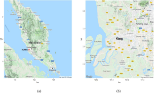
Bayesian network reasoning and machine learning with multiple data features: air pollution risk monitoring and early warning

Air pollution prediction with machine learning: a case study of Indian cities

Air Pollution Prediction Using Extreme Learning Machine: A Case Study on Delhi (India)

Data availability.

Due to confidentiality agreements, supporting data can only be made available to bona fide researcher’s subject to a non-disclosure agreement. Details of the data and how to request access are available from https://www.doe.gov.my/portalv1/en/ at Department of Environment Malaysia.

Code availability

All code for Bayes naïve classification associated with the current submission is available at. https://cran.r-project.org/web/packages/e1071/index.html

Berrar, D. (2018). Bayes’ theorem and naive Bayes classifier. In S. Ranganathan, K. Nakai, & C. Schonbach (Eds.), Encyclopedia of Bioinformatics and Computational Biology: ABC of Bioinformatics. Amsterdam: Elsevier.

Google Scholar  

Catal, C., Sevim, U., & Diri, B. (2011). Practical development of an Eclipse-based software fault prediction tool using Naive Bayes algorithm. Expert Systems with Applications, 38 (3), 2347–2353. https://doi.org/10.1016/j.eswa.2010.08.022

Article   Google Scholar  

Chandra, B., & Sharma, R. K. (2016). Fast learning in deep neural networks. Neurocomputing, 171 , 1205–1215. https://doi.org/10.1016/j.neucom.2015.07.093

Chen, J., Huang, H., Tian, S., & Qu, Y. (2009). Feature selection for text classification with Naïve Bayes. Expert Systems with Applications 36(3). Part, 1 , 5432–5435. https://doi.org/10.1016/j.eswa.2008.06.054

Chukwudum, Q. C., & Nadarajah, S. (2022). Bivariate extreme value analysis of rainfall and temperature in Nigeria. Environmental Modeling & Assessment, 27 , 343–362. https://doi.org/10.1007/s10666-021-09781-7

Corani, G., & Scanagatta, M. (2016). Air pollution prediction via multi-label classification. Environmental Modelling & Software, 80 , 259–264. https://doi.org/10.1016/j.envsoft.2016.02.030

Dai, H., Huang, G., & Zeng, H. (2023a). Multi-objective optimal dispatch strategy for power systems with spatio-temporal distribution of air pollutants. Sustainable Cities and Society, 98 , 104801. https://doi.org/10.1016/j.scs.2023.104801

Dai, H., Huang, G., Wang, J., & Zeng, H. (2023b). VAR-tree model based spatio-temporal characterization and prediction of O 3 concentration in China. Ecotoxicology and Environmental Safety, 257 , 114960. https://doi.org/10.1016/j.ecoenv.2023.114960

Article   CAS   Google Scholar  

Dedoussi, I. C., Eastham, S. D., Monier, E., & Barret, S. R. H. (2020). Premature mortality related to United States cross-state air pollution. Nature, 578 , 261–265. https://doi.org/10.1038/s41586-020-1983-8

Department of Environment. (1997). A guide to air pollutant index in Malaysia (API). Kuala Lumpur, Malaysia. Ministry of Science, Technology and the Environment. https://aqicn.org/images/aqi-scales/malaysia-api-guide.pdf . Accessed on 13 Feb 2023

Elgeldawi, E., Sayed, A., Galal, A. R., & Zaki, A. M. (2021). Hyperparameter tuning for machine learning algorithms used for arabic sentiment analysis. Informatics, 8 , 79. https://doi.org/10.3390/informatics8040079

Flach, P. A., & Lachiche, N. (2004). Naive Bayesian classification of structured data. Machine Learning, 57 , 233–269. https://doi.org/10.1023/B:MACH.0000039778.69032.ab

Glick, M., Klon, A. E., Acklin, P., & Davies, J. W. (2004). Enrichment of extremely noisy high-throughput screening data using a naïve Bayes classifier. JOurnal of Biomolecular Screening, 9 (1), 32–36. https://doi.org/10.1177/1087057103260590

Google. (2019) https://maps.googleapis.com/maps/api/geocode/json?address=Klang%2CSelangor&key=xxx . Accessed on 13 April 2022

Guo, Y., Liu, Y., Oerlemans, A., Lao, S., Wu, S., & Lew, M. S. (2016). Deep learning for visual understanding: A review. Neurocomputing, 187 , 27–48. https://doi.org/10.1016/j.neucom.2015.09.116

Hähnel, P., Mareček, J., Monteil, J., & O’Donncha, F. (2020). Using deep learning to extend the range of air pollution monitoring and forecasting. Journal of Computational Physics, 408 , 109278. https://doi.org/10.1016/j.jcp.2020.109278

Harzevili, N. S., & Alizadeh, S. H. (2018). Mixture of latent multinomial naive Bayes classifier. Applied Soft Computing, 69 , 516–527. https://doi.org/10.1016/j.asoc.2018.04.020

Heard, N. (2021). An introduction to Bayesian inference: Methods and computation . Springer.

Hoffmann, C., Maglakelidze, M., von Schneidemesser, E., Witt, C., Hoffmann, P., & Butler, T. (2022). Asthma and COPD exacerbation in relation to outdoor air pollution in the metropolitan area of Berlin. Germany. Respiratory Research, 23 , 64. https://doi.org/10.1186/s12931-022-01983-1

Humpherys, S. L., Moffitt, K. C., Burns, M. B., Burgoon, J. K., & Felix, W. F. (2011). Identification of fraudulent financial statements using linguistic credibility analysis. Decision Support Systems, 50 (3), 585–594. https://doi.org/10.1016/j.dss.2010.08.009

Jin, Y., O’Connor, D., Ok, Y. S., Tsang, D. C. W., Liu, A., & Hou, D. (2019). Assessment of sources of heavy metals in soil and dust at children’s playgrounds in Beijing using GIS and multivariate statistical analysis. Environment International, 124 , 320–328. https://doi.org/10.1016/j.envint.2019.01.024

Kahloot, K. M., & Ekler, P. (2021). Algorithmic splitting: A method for dataset preparation. IEEE Access, 9 , 125229–125237. https://doi.org/10.1109/ACCESS.2021.3110745

Kamińska, J. A. (2018). The use of random forests in modelling short-term air pollution effects based on traffic and meteorological conditions: A case study in Wrocław. Journal of Environmental Management, 217 , 164–174. https://doi.org/10.1016/j.jenvman.2018.03.094

Kazmierska, J., & Malicki, J. (2008). Application of the Naïve Bayesian Classifier to optimize treatment decisions. Radiotherapy and Oncology, 86 (2), 211–216. https://doi.org/10.1016/j.radonc.2007.10.019

Lantz, B. (2019). Machine learning with R: Expert techniques for predictive modeling (3rd ed.). Packt Publishing Ltd.

Lee, M., Lin, L., Chen, C. Y., Tsao, Y., Yao, T.-H., Fei, M.-H., & Fang, S.-H. (2020). Forecasting air quality in Taiwan by using machine learning. Scientific Reports, 10 , 4153. https://doi.org/10.1038/s41598-020-61151-7

Leong, W. C., Kelani, R. O., & Ahmad, Z. (2020). Prediction of air pollution index (API) using support vector machine (SVM). Journal of Environmental Chemical Engineering, 8 (3), 103208. https://doi.org/10.1016/j.jece.2019.103208

Liao, Q., Zhu, M., Wu, L., Pan, X., Tang, X., & Wang, Z. (2020). Deep learning for air quality forecasts: A review. Current Pollution Reports, 6 , 399–409. https://doi.org/10.1007/s40726-020-00159-z

Lin, C.-Y., Chang, Y.-S., & Abimannan, S. (2021). Ensemble multifeatured deep learning models for air quality forecasting. Atmospheric Pollution Research, 12 (5), 101045. https://doi.org/10.1016/j.apr.2021.03.008

Liu, B., Yang, Y., Webb, G. I., Boughton, J. (2009). A comparative study of bandwidth choice in kernel density estimation for naive Bayesian classification. In: Theeramunkong, T., Kijsirikul, B., Cercone, N., Ho, TB. (eds) Advances in Knowledge Discovery and Data Mining . PAKDD 2009. Lecture Notes in Computer Science, vol 5476. Springer, Berlin, Heidelberg. https://doi.org/10.1007/978-3-642-01307-2_29

Lu, W.-Z., & Wang, W.-J. (2005). Potential assessment of the “support vector machine” method in forecasting ambient air pollutant trends. Chemosphere, 59 (5), 693–701. https://doi.org/10.1016/j.chemosphere.2004.10.032

Lu, Y., Cheung, Y.-M., & Tang, Y. Y. (2020). Bayes imbalance impact index: A measure of class imbalanced data set for classification problem. IEEE Transactions on Neural Networks and Learning Systems, 31 (9), 3525–3539. https://doi.org/10.1109/TNNLS.2019.2944962

Masseran, N. (2017). Modeling fluctuation of PM 10 data with existence of volatility effect. Environmental Engineering Science, 34 (11), 816–827. https://doi.org/10.1089/ees.2016.0448

Masseran, N. (2021). Power-law behaviors of the duration size of unhealthy air pollution events. Stochastic Environmental Research and Risk Assessment, 35 , 1499–1508. https://doi.org/10.1007/s00477-021-01978-2

Masseran, N. (2022a). Power-law behaviors of the severity of unhealthy air pollution events. Natural Hazards, 112 , 1749–1766. https://doi.org/10.1007/s11069-022-05247-5

Masseran, N. (2022b). Multifractal characteristics on multiple pollution variables in Malaysia. Bulletin of the Malaysian Mathematical Sciences Society, 45 , 325–344. https://doi.org/10.1007/s40840-022-01304-1

Masseran, N., & Hussain, S. I. (2020). Copula modelling on the dynamic dependence structure of multiple air pollutant variables. Mathematics, 8 (11), 1910. https://doi.org/10.3390/math8111910

Masseran, N., & Mohd Safari, M. A. (2020). Intensity–duration–frequency approach for risk assessment of air pollution events. Journal of Environmental Management, 264 , 110429. https://doi.org/10.1016/j.jenvman.2020.110429

Masseran, N., & Safari, M. A. M. (2021). Mixed POT-BM approach for modeling unhealthy air pollution events. International Journal of Environmental Research and Public Health, 18 (13), 6754. https://doi.org/10.3390/ijerph18136754

Masseran, N., Razali, A. M., Ibrahim, K., & Latif, M. T. (2016). Modeling air quality in main cities of Peninsular Malaysia by using a generalized Pareto model. Environmental Monitoring and Assessment, 188 (1), 1–12. https://doi.org/10.1007/s10661-015-5070-9

Masseran, N., Tajuddin, R. R. M., & Latif, M. T. (2023). Classifying severity of unhealthy air pollution events in Malaysia: A decision tree model. Sains Malaysiana, 52 (10), 2971–2983. https://doi.org/10.17576/jsm-2023-5210-18

Méndez, M., Merayo, M. G., & Núñez, M. (2023). Machine learning algorithms to forecast air quality: A survey. Artificial Intelligence Review, 56 , 10031–10066. https://doi.org/10.1007/s10462-023-10424-4

Muralidharan, V., & Sugumaran, V. (2012). A comparative study of Naïve Bayes classifier and Bayes net classifier for fault diagnosis of monoblock centrifugal pump using wavelet analysis. Applied Soft Computing, 12 (8), 2023–2029. https://doi.org/10.1016/j.asoc.2012.03.021

Murphy, K. P. (2022). Probabilistic machine learning: An introduction . The MIT Press.

Ouyang, X., Shao, X., Zhu, X, He, Q., Xiang, C., Wei, G. (2019). Environmental regulation, economic growth and air pollution: Panel threshold analysis for OECD countries. Science of the total environment, 657 , 234–241. https://doi.org/10.1016/j.scitotenv.2018.12.056

Sakia, R. M. (1992). The Box-Cox transformation technique: A review. Journal of the Royal Statistical Society: Series D, 41 (2), 169–178. https://doi.org/10.2307/2348250

Soria, D., Garibaldi, J. M., Ambrogi, F., Biganzoli, E. M., & Ellis, I. O. (2011). A ‘non-parametric’ version of the naive Bayes classifier. Knowledge-Based Systems, 24 (6), 775–784. https://doi.org/10.1016/j.knosys.2011.02.014

Suhaimi, N. F., Jalaludin, J., & Juhari, M. A. M. (2020). The impact of traffic-related air pollution on lung function status and respiratory symptoms among children in Klang Valley, Malaysia. International Journal of Environmental Health Research, 32 (3), 535–546. https://doi.org/10.1080/09603123.2020.1784397

Vadrevu, K. P., Eaturu, A., Biswas, S., Lasko, K., Sahu, S., Garg, J. K., & Justice, C. (2020). Spatial and temporal variations of air pollution over 41 cities of India during the COVID-19 lockdown period. Scientific Reports, 10 , 16574. https://doi.org/10.1038/s41598-020-72271-5

Valle, M. A., Varas, S., & Ruz, G. A. (2012). Job performance prediction in a call center using a naive Bayes classifier. Expert Systems with Applications, 39 (11), 9939–9945. https://doi.org/10.1016/j.eswa.2011.11.126

van Oijen, M. (2020). Bayesian Compendium . Springer.

Book   Google Scholar  

Wang, Y., Ying, Q., Hu, J., & Zhang, H. (2014). Spatial and temporal variations of six criteria air pollutants in 31 provincial capital cities in China during 2013–2014. Environment International, 73 , 413–422. https://doi.org/10.1016/j.envint.2014.08.016

Webb, G. I. (2011). Naïve Bayes. In C. Sammut & G. I. Webb (Eds.), Encyclopedia of Machine Learning. Boston: Springer. https://doi.org/10.1007/978-0-387-30164-8_576

Chapter   Google Scholar  

Wickramasinghe, I., & Kalutarage, H. (2021). Naive Bayes: Applications, variations and vulnerabilities: A review of literature with code snippets for implementation. Soft Computing, 25 , 2277–2293. https://doi.org/10.1007/s00500-020-05297-6

Xu, S. (2018). Bayesian naive Bayes classifiers to text classification. Journal of Information Science, 44 (1), 48–59. https://doi.org/10.1177/0165551516677946

Xu, G., Ren, X., Xiong, K., Li, L., Bi, X., Wu, Q. (2020). Analysis of the driving factors of PM2.5 concentration in the air: A case study of the Yangtze River Delta, China. Ecological Indicators 110, 105889 https://doi.org/10.1016/j.ecolind.2019.105889

Yang, L., & Shami, A. (2020). On hyperparameter optimization of machine learning algorithms: Theory and practice. Neurocomputing, 415 , 295–316. https://doi.org/10.1016/j.neucom.2020.07.061

Yang, B.-Y., Fan, S., Thiering, E., Seissler, J., Nowak, D., Dong, G.-H., & Heinrich, J. (2020). Ambient air pollution and diabetes: A systematic review and meta-analysis. Environmental Research, 180 , 108817. https://doi.org/10.1016/j.envres.2019.108817

Yang, Q., Gu, Y., Wu, D. (2019). Survey of incremental learning. 2019 Chinese Control and Decision Conference (CCDC), Nanchang, China , pp. 399–404

Yi, H., Xiong, Q., Zou, Q., Xu, R., Wang, K., Gao, M. (2019). A novel random forest and its application on classification of air quality. In 2019 8th International Congress on Advanced Applied Informatics (IIAI-AAI) . Toyama, Japan, pp. 35–38

Zaki, M. J., & Meira, W., Jr. (2020). Data Mining and Machine Learning: Fundamental Concepts and Algorithms (2nd ed.). Cambridge University Press.

Zhang, H., Liu, R., Liu, J., & Zhang, Z. (2022a). Formal probabilistic risk analysis of accidental air pollution in a development zone using Bayesian networks. Journal of Cleaner Production, 372 , 133774. https://doi.org/10.1016/j.jclepro.2022.133774

Zhang, Z., Zhang, G., & Su, B. (2022b). The spatial impacts of air pollution and socio-economic status on public health: Empirical evidence from China. Socio-Economic Planning Sciences, 83 , 101167. https://doi.org/10.1016/j.seps.2021.101167

Download references

Acknowledgements

The author is indebted to the Malaysian Department of Environment for providing air pollution data. This research would not be possible without the sponsorship from the Universiti Kebangsaan Malaysia (grant number GP-K020446).

This work is supported by the Universiti Kebangsaan Malaysia [grant number GP-K020446].

Author information

Authors and affiliations.

Department of Mathematical Sciences, Faculty of Science and Technology, Universiti Kebangsaan Malaysia, UKM, 43600, Bangi, Selangor, Malaysia

Nurulkamal Masseran & Razik Ridzuan Mohd Tajuddin

Department of Mathematics and Statistics, Faculty of Science, Universiti Putra Malaysia, 43400 UPM, Serdang, Selangor, Malaysia

Muhammad Aslam Mohd Safari

You can also search for this author in PubMed   Google Scholar

Contributions

NKM conceived of the presented idea and performed the analysis. MAMS and RRMT have verified the analytical methods. All authors discussed the results and contributed to the final manuscript.‬‬‬‬‬

Corresponding author

Correspondence to Nurulkamal Masseran .

Ethics declarations

Competing interests.

The authors declare no competing interests.

Conflict of interest

Ethics approval.

Not applicable.

Consent to participate

Consent for publication, additional information, publisher's note.

Springer Nature remains neutral with regard to jurisdictional claims in published maps and institutional affiliations.

Rights and permissions

Springer Nature or its licensor (e.g. a society or other partner) holds exclusive rights to this article under a publishing agreement with the author(s) or other rightsholder(s); author self-archiving of the accepted manuscript version of this article is solely governed by the terms of such publishing agreement and applicable law.

Reprints and permissions

About this article

Masseran, N., Safari, M.A.M. & Tajuddin, R.R.M. Probabilistic classification of the severity classes of unhealthy air pollution events. Environ Monit Assess 196 , 523 (2024). https://doi.org/10.1007/s10661-024-12700-4

Download citation

Received : 05 October 2023

Accepted : 30 April 2024

Published : 08 May 2024

DOI : https://doi.org/10.1007/s10661-024-12700-4

Share this article

Anyone you share the following link with will be able to read this content:

Sorry, a shareable link is not currently available for this article.

Provided by the Springer Nature SharedIt content-sharing initiative

• Air pollution classification
• Extreme severity
• Pollution risk assessment
• Probabilistic predictive
• Find a journal
• Publish with us
• Track your research