different methods of data presentation pdf

An official website of the United States government

The .gov means it’s official. Federal government websites often end in .gov or .mil. Before sharing sensitive information, make sure you’re on a federal government site.

The site is secure. The https:// ensures that you are connecting to the official website and that any information you provide is encrypted and transmitted securely.

• Publications
• Account settings

Preview improvements coming to the PMC website in October 2024. Learn More or Try it out now .

• Advanced Search
• Journal List
• Korean J Anesthesiol
• v.70(3); 2017 Jun

Statistical data presentation

1 Department of Anesthesiology and Pain Medicine, Dongguk University Ilsan Hospital, Goyang, Korea.

Sangseok Lee

2 Department of Anesthesiology and Pain Medicine, Sanggye Paik Hospital, Inje University College of Medicine, Seoul, Korea.

Data are usually collected in a raw format and thus the inherent information is difficult to understand. Therefore, raw data need to be summarized, processed, and analyzed. However, no matter how well manipulated, the information derived from the raw data should be presented in an effective format, otherwise, it would be a great loss for both authors and readers. In this article, the techniques of data and information presentation in textual, tabular, and graphical forms are introduced. Text is the principal method for explaining findings, outlining trends, and providing contextual information. A table is best suited for representing individual information and represents both quantitative and qualitative information. A graph is a very effective visual tool as it displays data at a glance, facilitates comparison, and can reveal trends and relationships within the data such as changes over time, frequency distribution, and correlation or relative share of a whole. Text, tables, and graphs for data and information presentation are very powerful communication tools. They can make an article easy to understand, attract and sustain the interest of readers, and efficiently present large amounts of complex information. Moreover, as journal editors and reviewers glance at these presentations before reading the whole article, their importance cannot be ignored.

Introduction

Data are a set of facts, and provide a partial picture of reality. Whether data are being collected with a certain purpose or collected data are being utilized, questions regarding what information the data are conveying, how the data can be used, and what must be done to include more useful information must constantly be kept in mind.

Since most data are available to researchers in a raw format, they must be summarized, organized, and analyzed to usefully derive information from them. Furthermore, each data set needs to be presented in a certain way depending on what it is used for. Planning how the data will be presented is essential before appropriately processing raw data.

First, a question for which an answer is desired must be clearly defined. The more detailed the question is, the more detailed and clearer the results are. A broad question results in vague answers and results that are hard to interpret. In other words, a well-defined question is crucial for the data to be well-understood later. Once a detailed question is ready, the raw data must be prepared before processing. These days, data are often summarized, organized, and analyzed with statistical packages or graphics software. Data must be prepared in such a way they are properly recognized by the program being used. The present study does not discuss this data preparation process, which involves creating a data frame, creating/changing rows and columns, changing the level of a factor, categorical variable, coding, dummy variables, variable transformation, data transformation, missing value, outlier treatment, and noise removal.

We describe the roles and appropriate use of text, tables, and graphs (graphs, plots, or charts), all of which are commonly used in reports, articles, posters, and presentations. Furthermore, we discuss the issues that must be addressed when presenting various kinds of information, and effective methods of presenting data, which are the end products of research, and of emphasizing specific information.

Data Presentation

Data can be presented in one of the three ways:

–as text;

–in tabular form; or

–in graphical form.

Methods of presentation must be determined according to the data format, the method of analysis to be used, and the information to be emphasized. Inappropriately presented data fail to clearly convey information to readers and reviewers. Even when the same information is being conveyed, different methods of presentation must be employed depending on what specific information is going to be emphasized. A method of presentation must be chosen after carefully weighing the advantages and disadvantages of different methods of presentation. For easy comparison of different methods of presentation, let us look at a table ( Table 1 ) and a line graph ( Fig. 1 ) that present the same information [ 1 ]. If one wishes to compare or introduce two values at a certain time point, it is appropriate to use text or the written language. However, a table is the most appropriate when all information requires equal attention, and it allows readers to selectively look at information of their own interest. Graphs allow readers to understand the overall trend in data, and intuitively understand the comparison results between two groups. One thing to always bear in mind regardless of what method is used, however, is the simplicity of presentation.

Values are expressed as mean ± SD. Group C: normal saline, Group D: dexmedetomidine. SBP: systolic blood pressure, DBP: diastolic blood pressure, MBP: mean blood pressure, HR: heart rate. * P < 0.05 indicates a significant increase in each group, compared with the baseline values. † P < 0.05 indicates a significant decrease noted in Group D, compared with the baseline values. ‡ P < 0.05 indicates a significant difference between the groups.

Text presentation

Text is the main method of conveying information as it is used to explain results and trends, and provide contextual information. Data are fundamentally presented in paragraphs or sentences. Text can be used to provide interpretation or emphasize certain data. If quantitative information to be conveyed consists of one or two numbers, it is more appropriate to use written language than tables or graphs. For instance, information about the incidence rates of delirium following anesthesia in 2016–2017 can be presented with the use of a few numbers: “The incidence rate of delirium following anesthesia was 11% in 2016 and 15% in 2017; no significant difference of incidence rates was found between the two years.” If this information were to be presented in a graph or a table, it would occupy an unnecessarily large space on the page, without enhancing the readers' understanding of the data. If more data are to be presented, or other information such as that regarding data trends are to be conveyed, a table or a graph would be more appropriate. By nature, data take longer to read when presented as texts and when the main text includes a long list of information, readers and reviewers may have difficulties in understanding the information.

Table presentation

Tables, which convey information that has been converted into words or numbers in rows and columns, have been used for nearly 2,000 years. Anyone with a sufficient level of literacy can easily understand the information presented in a table. Tables are the most appropriate for presenting individual information, and can present both quantitative and qualitative information. Examples of qualitative information are the level of sedation [ 2 ], statistical methods/functions [ 3 , 4 ], and intubation conditions [ 5 ].

The strength of tables is that they can accurately present information that cannot be presented with a graph. A number such as “132.145852” can be accurately expressed in a table. Another strength is that information with different units can be presented together. For instance, blood pressure, heart rate, number of drugs administered, and anesthesia time can be presented together in one table. Finally, tables are useful for summarizing and comparing quantitative information of different variables. However, the interpretation of information takes longer in tables than in graphs, and tables are not appropriate for studying data trends. Furthermore, since all data are of equal importance in a table, it is not easy to identify and selectively choose the information required.

For a general guideline for creating tables, refer to the journal submission requirements 1) .

Heat maps for better visualization of information than tables

Heat maps help to further visualize the information presented in a table by applying colors to the background of cells. By adjusting the colors or color saturation, information is conveyed in a more visible manner, and readers can quickly identify the information of interest ( Table 2 ). Software such as Excel (in Microsoft Office, Microsoft, WA, USA) have features that enable easy creation of heat maps through the options available on the “conditional formatting” menu.

All numbers were created by the author. SBP: systolic blood pressure, DBP: diastolic blood pressure, MBP: mean blood pressure, HR: heart rate.

Graph presentation

Whereas tables can be used for presenting all the information, graphs simplify complex information by using images and emphasizing data patterns or trends, and are useful for summarizing, explaining, or exploring quantitative data. While graphs are effective for presenting large amounts of data, they can be used in place of tables to present small sets of data. A graph format that best presents information must be chosen so that readers and reviewers can easily understand the information. In the following, we describe frequently used graph formats and the types of data that are appropriately presented with each format with examples.

Scatter plot

Scatter plots present data on the x - and y -axes and are used to investigate an association between two variables. A point represents each individual or object, and an association between two variables can be studied by analyzing patterns across multiple points. A regression line is added to a graph to determine whether the association between two variables can be explained or not. Fig. 2 illustrates correlations between pain scoring systems that are currently used (PSQ, Pain Sensitivity Questionnaire; PASS, Pain Anxiety Symptoms Scale; PCS, Pain Catastrophizing Scale) and Geop-Pain Questionnaire (GPQ) with the correlation coefficient, R, and regression line indicated on the scatter plot [ 6 ]. If multiple points exist at an identical location as in this example ( Fig. 2 ), the correlation level may not be clear. In this case, a correlation coefficient or regression line can be added to further elucidate the correlation.

Bar graph and histogram

A bar graph is used to indicate and compare values in a discrete category or group, and the frequency or other measurement parameters (i.e. mean). Depending on the number of categories, and the size or complexity of each category, bars may be created vertically or horizontally. The height (or length) of a bar represents the amount of information in a category. Bar graphs are flexible, and can be used in a grouped or subdivided bar format in cases of two or more data sets in each category. Fig. 3 is a representative example of a vertical bar graph, with the x -axis representing the length of recovery room stay and drug-treated group, and the y -axis representing the visual analog scale (VAS) score. The mean and standard deviation of the VAS scores are expressed as whiskers on the bars ( Fig. 3 ) [ 7 ].

By comparing the endpoints of bars, one can identify the largest and the smallest categories, and understand gradual differences between each category. It is advised to start the x - and y -axes from 0. Illustration of comparison results in the x - and y -axes that do not start from 0 can deceive readers' eyes and lead to overrepresentation of the results.

One form of vertical bar graph is the stacked vertical bar graph. A stack vertical bar graph is used to compare the sum of each category, and analyze parts of a category. While stacked vertical bar graphs are excellent from the aspect of visualization, they do not have a reference line, making comparison of parts of various categories challenging ( Fig. 4 ) [ 8 ].

A pie chart, which is used to represent nominal data (in other words, data classified in different categories), visually represents a distribution of categories. It is generally the most appropriate format for representing information grouped into a small number of categories. It is also used for data that have no other way of being represented aside from a table (i.e. frequency table). Fig. 5 illustrates the distribution of regular waste from operation rooms by their weight [ 8 ]. A pie chart is also commonly used to illustrate the number of votes each candidate won in an election.

Line plot with whiskers

A line plot is useful for representing time-series data such as monthly precipitation and yearly unemployment rates; in other words, it is used to study variables that are observed over time. Line graphs are especially useful for studying patterns and trends across data that include climatic influence, large changes or turning points, and are also appropriate for representing not only time-series data, but also data measured over the progression of a continuous variable such as distance. As can be seen in Fig. 1 , mean and standard deviation of systolic blood pressure are indicated for each time point, which enables readers to easily understand changes of systolic pressure over time [ 1 ]. If data are collected at a regular interval, values in between the measurements can be estimated. In a line graph, the x-axis represents the continuous variable, while the y-axis represents the scale and measurement values. It is also useful to represent multiple data sets on a single line graph to compare and analyze patterns across different data sets.

Box and whisker chart

A box and whisker chart does not make any assumptions about the underlying statistical distribution, and represents variations in samples of a population; therefore, it is appropriate for representing nonparametric data. AA box and whisker chart consists of boxes that represent interquartile range (one to three), the median and the mean of the data, and whiskers presented as lines outside of the boxes. Whiskers can be used to present the largest and smallest values in a set of data or only a part of the data (i.e. 95% of all the data). Data that are excluded from the data set are presented as individual points and are called outliers. The spacing at both ends of the box indicates dispersion in the data. The relative location of the median demonstrated within the box indicates skewness ( Fig. 6 ). The box and whisker chart provided as an example represents calculated volumes of an anesthetic, desflurane, consumed over the course of the observation period ( Fig. 7 ) [ 9 ].

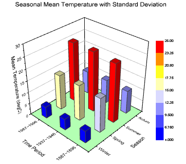
Three-dimensional effects

Most of the recently introduced statistical packages and graphics software have the three-dimensional (3D) effect feature. The 3D effects can add depth and perspective to a graph. However, since they may make reading and interpreting data more difficult, they must only be used after careful consideration. The application of 3D effects on a pie chart makes distinguishing the size of each slice difficult. Even if slices are of similar sizes, slices farther from the front of the pie chart may appear smaller than the slices closer to the front ( Fig. 8 ).

Drawing a graph: example

Finally, we explain how to create a graph by using a line graph as an example ( Fig. 9 ). In Fig. 9 , the mean values of arterial pressure were randomly produced and assumed to have been measured on an hourly basis. In many graphs, the x- and y-axes meet at the zero point ( Fig. 9A ). In this case, information regarding the mean and standard deviation of mean arterial pressure measurements corresponding to t = 0 cannot be conveyed as the values overlap with the y-axis. The data can be clearly exposed by separating the zero point ( Fig. 9B ). In Fig. 9B , the mean and standard deviation of different groups overlap and cannot be clearly distinguished from each other. Separating the data sets and presenting standard deviations in a single direction prevents overlapping and, therefore, reduces the visual inconvenience. Doing so also reduces the excessive number of ticks on the y-axis, increasing the legibility of the graph ( Fig. 9C ). In the last graph, different shapes were used for the lines connecting different time points to further allow the data to be distinguished, and the y-axis was shortened to get rid of the unnecessary empty space present in the previous graphs ( Fig. 9D ). A graph can be made easier to interpret by assigning each group to a different color, changing the shape of a point, or including graphs of different formats [ 10 ]. The use of random settings for the scale in a graph may lead to inappropriate presentation or presentation of data that can deceive readers' eyes ( Fig. 10 ).

Owing to the lack of space, we could not discuss all types of graphs, but have focused on describing graphs that are frequently used in scholarly articles. We have summarized the commonly used types of graphs according to the method of data analysis in Table 3 . For general guidelines on graph designs, please refer to the journal submission requirements 2) .

Conclusions

Text, tables, and graphs are effective communication media that present and convey data and information. They aid readers in understanding the content of research, sustain their interest, and effectively present large quantities of complex information. As journal editors and reviewers will scan through these presentations before reading the entire text, their importance cannot be disregarded. For this reason, authors must pay as close attention to selecting appropriate methods of data presentation as when they were collecting data of good quality and analyzing them. In addition, having a well-established understanding of different methods of data presentation and their appropriate use will enable one to develop the ability to recognize and interpret inappropriately presented data or data presented in such a way that it deceives readers' eyes [ 11 ].

<Appendix>

Output for presentation.

Discovery and communication are the two objectives of data visualization. In the discovery phase, various types of graphs must be tried to understand the rough and overall information the data are conveying. The communication phase is focused on presenting the discovered information in a summarized form. During this phase, it is necessary to polish images including graphs, pictures, and videos, and consider the fact that the images may look different when printed than how appear on a computer screen. In this appendix, we discuss important concepts that one must be familiar with to print graphs appropriately.

The KJA asks that pictures and images meet the following requirement before submission 3)

“Figures and photographs should be submitted as ‘TIFF’ files. Submit files of figures and photographs separately from the text of the paper. Width of figure should be 84 mm (one column). Contrast of photos or graphs should be at least 600 dpi. Contrast of line drawings should be at least 1,200 dpi. The Powerpoint file (ppt, pptx) is also acceptable.”

Unfortunately, without sufficient knowledge of computer graphics, it is not easy to understand the submission requirement above. Therefore, it is necessary to develop an understanding of image resolution, image format (bitmap and vector images), and the corresponding file specifications.

Resolution is often mentioned to describe the quality of images containing graphs or CT/MRI scans, and video files. The higher the resolution, the clearer and closer to reality the image is, while the opposite is true for low resolutions. The most representative unit used to describe a resolution is “dpi” (dots per inch): this literally translates to the number of dots required to constitute 1 inch. The greater the number of dots, the higher the resolution. The KJA submission requirements recommend 600 dpi for images, and 1,200 dpi 4) for graphs. In other words, resolutions in which 600 or 1,200 dots constitute one inch are required for submission.

There are requirements for the horizontal length of an image in addition to the resolution requirements. While there are no requirements for the vertical length of an image, it must not exceed the vertical length of a page. The width of a column on one side of a printed page is 84 mm, or 3.3 inches (84/25.4 mm ≒ 3.3 inches). Therefore, a graph must have a resolution in which 1,200 dots constitute 1 inch, and have a width of 3.3 inches.

Bitmap and Vector

Methods of image construction are important. Bitmap images can be considered as images drawn on section paper. Enlarging the image will enlarge the picture along with the grid, resulting in a lower resolution; in other words, aliasing occurs. On the other hand, reducing the size of the image will reduce the size of the picture, while increasing the resolution. In other words, resolution and the size of an image are inversely proportionate to one another in bitmap images, and it is a drawback of bitmap images that resolution must be considered when adjusting the size of an image. To enlarge an image while maintaining the same resolution, the size and resolution of the image must be determined before saving the image. An image that has already been created cannot avoid changes to its resolution according to changes in size. Enlarging an image while maintaining the same resolution will increase the number of horizontal and vertical dots, ultimately increasing the number of pixels 5) of the image, and the file size. In other words, the file size of a bitmap image is affected by the size and resolution of the image (file extensions include JPG [JPEG] 6) , PNG 7) , GIF 8) , and TIF [TIFF] 9) . To avoid this complexity, the width of an image can be set to 4 inches and its resolution to 900 dpi to satisfy the submission requirements of most journals [ 12 ].

Vector images overcome the shortcomings of bitmap images. Vector images are created based on mathematical operations of line segments and areas between different points, and are not affected by aliasing or pixelation. Furthermore, they result in a smaller file size that is not affected by the size of the image. They are commonly used for drawings and illustrations (file extensions include EPS 10) , CGM 11) , and SVG 12) ).

Finally, the PDF 13) is a file format developed by Adobe Systems (Adobe Systems, CA, USA) for electronic documents, and can contain general documents, text, drawings, images, and fonts. They can also contain bitmap and vector images. While vector images are used by researchers when working in Powerpoint, they are saved as 960 × 720 dots when saved in TIFF format in Powerpoint. This results in a resolution that is inappropriate for printing on a paper medium. To save high-resolution bitmap images, the image must be saved as a PDF file instead of a TIFF, and the saved PDF file must be imported into an imaging processing program such as Photoshop™(Adobe Systems, CA, USA) to be saved in TIFF format [ 12 ].

1) Instructions to authors in KJA; section 5-(9) Table; https://ekja.org/index.php?body=instruction

2) Instructions to Authors in KJA; section 6-1)-(10) Figures and illustrations in Manuscript preparation; https://ekja.org/index.php?body=instruction

3) Instructions to Authors in KJA; section 6-1)-(10) Figures and illustrations in Manuscript preparation; https://ekja.org/index.php?body=instruction

4) Resolution; in KJA, it is represented by “contrast.”

5) Pixel is a minimum unit of an image and contains information of a dot and color. It is derived by multiplying the number of vertical and horizontal dots regardless of image size. For example, Full High Definition (FHD) monitor has 1920 × 1080 dots ≒ 2.07 million pixel.

6) Joint Photographic Experts Group.

7) Portable Network Graphics.

8) Graphics Interchange Format

9) Tagged Image File Format; TIFF

10) Encapsulated PostScript.

11) Computer Graphics Metafile.

12) Scalable Vector Graphics.

13) Portable Document Format.

Data Presentation

Josée Dupuis, PhD, Professor of Biostatistics, Boston University School of Public Health

Wayne LaMorte, MD, PhD, MPH, Professor of Epidemiology, Boston University School of Public Health

Introduction

While graphical summaries of data can certainly be powerful ways of communicating results clearly and unambiguously in a way that facilitates our ability to think about the information, poorly designed graphical displays can be ambiguous, confusing, and downright misleading. The keys to excellence in graphical design and communication are much like the keys to good writing. Adhere to fundamental principles of style and communicate as logically, accurately, and clearly as possible. Excellence in writing is generally achieved by avoiding unnecessary words and paragraphs; it is efficient. In a similar fashion, excellence in graphical presentation is generally achieved by efficient designs that avoid unnecessary ink.

Excellence in graphical presentation depends on:

• Choosing the best medium for presenting the information
• Designing the components of the graph in a way that communicates the information as clearly and accurately as possible.

Table or Graph?

• Tables are generally best if you want to be able to look up specific information or if the values must be reported precisely.
• Graphics are best for illustrating trends and making comparisons

The side by side illustrations below show the same information, first in table form and then in graphical form. While the information in the table is precise, the real goal is to compare a series of clinical outcomes in subjects taking either a drug or a placebo. The graphical presentation on the right makes it possible to quickly see that for each of the outcomes evaluated, the drug produced relief in a great proportion of subjects. Moreover, the viewer gets a clear sense of the magnitude of improvement, and the error bars provided a sense of the uncertainty in the data.

Principles for Table Display

• Sort table rows in a meaningful way
• Avoid alphabetical listing!
• Use rates, proportions or ratios in addition (or instead of) totals
• Show more than two time points if available
• Multiple time points may be better presented in a Figure
• Similar data should go down columns
• Highlight important comparisons
• Show the source of the data

Consider the data in the table below from http://www.cancer.gov/cancertopics/types/commoncancers

Our ability to quickly understand the relative frequency of these cancers is hampered by presenting them in alphabetical order. It is much easier for the reader to grasp the relative frequency by listing them from most frequent to least frequent as in the next table.

However, the same information might be presented more effectively with a dot plot, as shown below.

Data from http://www.cancer.gov/cancertopics/types/commoncancers

Principles of Graphical Excellence from E.R. Tufte

Pattern perception.

Pattern perception is done by

• Detection: recognition of geometry encoding physical values
• Assembly: grouping of detected symbol elements; discerning overall patterns in data
• Estimation: assessment of relative magnitudes of two physical values

Geographic Variation in Cancer

As an example, Tufte offers a series of maps that summarize the age-adjusted mortality rates for various types of cancer in the 3,056 counties in the United States. The maps showing the geographic variation in stomach cancer are shown below.

These maps summarize an enormous amount of information and present it efficiently, coherently, and effectively.in a way that invites the viewer to make comparisons and to think about the substance of the findings. Consider, for example, that the region to the west of the Great Lakes was settled largely by immigrants from Germany and Scand anavia, where traditional methods of preserving food included pickling and curing of fish by smoking. Could these methods be associated with an increased risk of stomach cancer?

John Snow's Spot Map of Cholera Cases

Consider also the spot map that John Snow presented after the cholera outbreak in the Broad Street section of London in September 1854. Snow ascertained the place of residence or work of the victims and represented them on a map of the area using a small black disk to represent each victim and stacking them when more than one occurred at a particular location. Snow reasoned that cholera was probably caused by something that was ingested, because of the intense diarrhea and vomiting of the victims, and he noted that the vast majority of cholera deaths occurred in people who lived or worked in the immediate vicinity of the broad street pump (shown with a red dot that we added for clarity). He further ascertained that most of the victims drank water from the Broad Street pump, and it was this evidence that persuaded the authorities to remove the handle from the pump in order to prevent more deaths.

Humans can readily perceive differences like this when presented effectively as in the two previous examples. However, humans are not good at estimating differences without directly seeing them (especially for steep curves), and we are particularly bad at perceiving relative angles (the principal perception task used in a pie chart).

The use of pie charts is generally discouraged. Consider the pie chart on the left below. It is difficult to accurately assess the relative size of the components in the pie chart, because the human eye has difficulty judging angles. The dot plot on the right shows the same data, but it is much easier to quickly assess the relative size of the components and how they changed from Fiscal Year 2000 to Fiscal Year 2007.

Consider the information in the two pie charts below (showing the same information).The 3-dimensional pie chart on the left distorts the relative proportions. In contrast the 2-dimensional pie chart on the right makes it much easier to compare the relative size of the varies components..

More Principles of Graphical Excellence

Exclude unneeded dimensions.

These 3-dimensional techniques distort the data and actually interfere with our ability to make accurate comparisons. The distortion caused by 3-dimensional elements can be particularly severe when the graphic is slanted at an angle or when the viewer tends to compare ends up unwittingly comparing the areas of the ink rather than the heights of the bars.

It is much easier to make comparisons with a chart like the one below.

Source: Huang, C, Guo C, Nichols C, Chen S, Martorell R. Elevated levels of protein in urine in adulthood after exposure to

the Chinese famine of 1959–61 during gestation and the early postnatal period. Int. J. Epidemiol. (2014) 43 (6): 1806-1814 .

Omit "Chart Junk"

Consider these two examples.

Here is a simple enumeration of the number of pets in a neighborhood. There is absolutely no reason to connect these counts with lines. This is, in fact, confusing and inappropriate and nothing more than "chart junk."

Source: http://www.go-education.com/free-graph-maker.html

Moiré Vibration

Moiré effects are sometimes used in modern art to produce the appearance of vibration and movement. However, when these effects are applied to statistical presentations, they are distracting and add clutter because the visual noise interferes with the interpretation of the data.

Tufte presents the example shown below from Instituto de Expansao Commercial, Brasil, Graphicos Estatisticas (Rio de Janeiro, 1929, p. 15).

 While the intention is to present quantitative information about the textile industry, the moiré effects do not add anything, and they are distracting, if not visually annoying.

Present Data to Facilitate Comparisons

Here is an attempt to compare catches of cod fish and crab across regions and to relate the variation to changes in water temperature. The problem here is that the Y-axes are vastly different, making it hard to sort out what's really going on. Even the Y-axes for temperature are vastly different.

http://seananderson.ca/courses/11-multipanel/multipanel.pdf1

The ability to make comparisons is greatly facilitated by using the same scales for axes, as illustrated below.

Data source: Dawber TR, Meadors GF, Moore FE Jr. Epidemiological approaches to heart disease:

the Framingham Study. Am J Public Health Nations Health. 1951;41(3):279-81. PMID: 14819398

It is also important to avoid distorting the X-axis. Note in the example below that the space between 0.05 to 0.1 is the same as space between 0.1 and 0.2.

Source: Park JH, Gail MH, Weinberg CR, et al. Distribution of allele frequencies and effect sizes and

their interrelationships for common genetic susceptibility variants. Proc Natl Acad Sci U S A. 2011; 108:18026-31.

Consider the range of the Y-axis. In the examples below there is no relevant information below $40,000, so it is not necessary to begin the Y-axis at 0. The graph on the right makes more sense.

Also, consider using a log scale. this can be particularly useful when presenting ratios as in the example below.

Source: Broman KW, Murray JC, Sheffield VC, White RL, Weber JL (1998) Comprehensive human genetic maps:

Individual and sex-specific variation in recombination. American Journal of Human Genetics 63:861-869, Figure 1

We noted earlier that pie charts make it difficult to see differences within a single pie chart, but this is particularly difficult when data is presented with multiple pie charts, as in the example below.

Source: Bell ML, et al. (2007) Spatial and temporal variation in PM2.5 chemical composition in the United States

for health effects studies. Environmental Health Perspectives 115:989-995, Figure 3

When multiple comparisons are being made, it is essential to use colors and symbols in a consistent way, as in this example.

Source: Manning AK, LaValley M, Liu CT, et al.  Meta-Analysis of Gene-Environment Interaction:

Joint Estimation of SNP and SNP x Environment Regression Coefficients.  Genet Epidemiol 2011, 35(1):11-8.

Avoid putting too many lines on the same chart. In the example below, the only thing that is readily apparent is that 1980 was a very hot summer.

Data from National Weather Service Weather Forecast Office at

http://www.srh.noaa.gov/tsa/?n=climo_tulyeartemp

Make Efficient Use of Space

Reduce the ratio of ink to information.

This isn't efficient, because this graphic is totally uninformative.

Source: Mykland P, Tierney L, Yu B (1995) Regeneration in Markov chain samplers.  Journal of the American Statistical Association 90:233-241, Figure 1

Bar graphs add ink without conveying any additional information, and they are distracting. The graph below on the left inappropriately uses bars which clutter the graph without adding anything. The graph on the right displays the same data, by does so more clearly and with less clutter.

Multiple Types of Information on the Same Figure

Choosing the best graph type, bar charts, error bars and dot plots.

As noted previously, bar charts can be problematic. Here is another one presenting means and error bars, but the error bars are misleading because they only extend in one direction. A better alternative would have been to to use full error bars with a scatter plot, as illustrated previously (right).

Consider the four graphs below presenting the incidence of cancer by type. The upper left graph unnecessary uses bars, which take up a lot of ink. This layout also ends up making the fonts for the types of cancer too small. Small font is also a problem for the dot plot at the upper right, and this one also has unnecessary grid lines across the entire width.

The graph at the lower left has more readable labels and uses a simple dot plot, but the rank order is difficult to figure out.

The graph at the lower right is clearly the best, since the labels are readable, the magnitude of incidence is shown clearly by the dot plots, and the cancers are sorted by frequency.

Single Continuous Numeric Variable

In this situation a cumulative distribution function conveys the most information and requires no grouping of the variable. A box plot will show selected quantiles effectively, and box plots are especially useful when stratifying by multiple categories of another variable.

Histograms are also possible. Consider the examples below.

Two Variables

 The two graphs below summarize BMI (Body Mass Index) measurements in four categories, i.e., younger and older men and women. The graph on the left shows the means and 95% confidence interval for the mean in each of the four groups. This is easy to interpret, but the viewer cannot see that the data is actually quite skewed. The graph on the right shows the same information presented as a box plot. With this presentation method one gets a better understanding of the skewed distribution and how the groups compare.

The next example is a scatter plot with a superimposed smoothed line of prediction. The shaded region embracing the blue line is a representation of the 95% confidence limits for the estimated prediction. This was created using "ggplot" in the R programming language.

Source: Frank E. Harrell Jr. on graphics:  http://biostat.mc.vanderbilt.edu/twiki/pub/Main/StatGraphCourse/graphscourse.pdf (page 121)

Multivariate Data

The example below shows the use of multiple panels.

Source: Cleveland S. The Elements of Graphing Data. Hobart Press, Summit, NJ, 1994.

Displaying Uncertainty

• Error bars showing confidence limits
• Confidence bands drawn using two lines
• Shaded confidence bands
• Bayesian credible intervals
• Bayesian posterior densities

Confidence Limits

Shaded Confidence Bands

Source: Frank E. Harrell Jr. on graphics:  http://biostat.mc.vanderbilt.edu/twiki/pub/Main/StatGraphCourse/graphscourse.pdf

Source: Tweedie RL and Mengersen KL. (1992) Br. J. Cancer 66: 700-705

Forest Plot

This is a Forest plot summarizing 26 studies of cigarette smoke exposure on risk of lung cancer. The sizes of the black boxes indicating the estimated odds ratio are proportional to the sample size in each study.

Data from Tweedie RL and Mengersen KL. (1992) Br. J. Cancer 66: 700-705

Summary Recommendations

• In general, avoid bar plots
• Avoid chart junk and the use of too much ink relative to the information you are displaying. Keep it simple and clear.
• Avoid pie charts, because humans have difficulty perceiving relative angles.
• Pay attention to scale, and make scales consistent.
• Explore several ways to display the data!

12 Tips on How to Display Data Badly

Adapted from Wainer H.  How to Display Data Badly.  The American Statistician 1984; 38: 137-147. 

• Show as few data as possible
• Hide what data you do show; minimize the data-ink ratio
• Ignore the visual metaphor altogether
• Only order matters
• Graph data out of context
• Change scales in mid-axis
• Emphasize the trivial;  ignore the important
• Jiggle the baseline
• Alphabetize everything.
• Make your labels illegible, incomplete, incorrect, and ambiguous.
• More is murkier: use a lot of decimal places and make your graphs three dimensional whenever possible.
• If it has been done well in the past, think of another way to do it

Additional Resources

• Stephen Few: Designing Effective Tables and Graphs. http://www.perceptualedge.com/images/Effective_Chart_Design.pdf
• Gary Klaas: Presenting Data: Tabular and graphic display of social indicators. Illinois State University, 2002. http://lilt.ilstu.edu/gmklass/pos138/datadisplay/sections/goodcharts.htm (Note: The web site will be discontinued to be replaced by the Just Plain Data Analysis site).

10 Methods of Data Presentation with 5 Great Tips to Practice, Best in 2024

Leah Nguyen • 05 April, 2024 • 17 min read

There are different ways of presenting data, so which one is suited you the most? You can end deathly boring and ineffective data presentation right now with our 10 methods of data presentation . Check out the examples from each technique!

Have you ever presented a data report to your boss/coworkers/teachers thinking it was super dope like you’re some cyber hacker living in the Matrix, but all they saw was a pile of static numbers that seemed pointless and didn’t make sense to them?

Understanding digits is rigid . Making people from non-analytical backgrounds understand those digits is even more challenging.

How can you clear up those confusing numbers in the types of presentation that have the flawless clarity of a diamond? So, let’s check out best way to present data. 💎

Table of Contents

• What are Methods of Data Presentations?
• #1 – Tabular

#3 – Pie chart

#4 – bar chart, #5 – histogram, #6 – line graph, #7 – pictogram graph, #8 – radar chart, #9 – heat map, #10 – scatter plot.

• 5 Mistakes to Avoid
• Best Method of Data Presentation

Frequently Asked Questions

More tips with ahaslides.

• Marketing Presentation
• Survey Result Presentation
• Types of Presentation

Start in seconds.

Get any of the above examples as templates. Sign up for free and take what you want from the template library!

What are Methods of Data Presentation?

The term ’data presentation’ relates to the way you present data in a way that makes even the most clueless person in the room understand. 

Some say it’s witchcraft (you’re manipulating the numbers in some ways), but we’ll just say it’s the power of turning dry, hard numbers or digits into a visual showcase that is easy for people to digest.

Presenting data correctly can help your audience understand complicated processes, identify trends, and instantly pinpoint whatever is going on without exhausting their brains.

Good data presentation helps…

• Make informed decisions and arrive at positive outcomes . If you see the sales of your product steadily increase throughout the years, it’s best to keep milking it or start turning it into a bunch of spin-offs (shoutout to Star Wars👀).
• Reduce the time spent processing data . Humans can digest information graphically 60,000 times faster than in the form of text. Grant them the power of skimming through a decade of data in minutes with some extra spicy graphs and charts.
• Communicate the results clearly . Data does not lie. They’re based on factual evidence and therefore if anyone keeps whining that you might be wrong, slap them with some hard data to keep their mouths shut.
• Add to or expand the current research . You can see what areas need improvement, as well as what details often go unnoticed while surfing through those little lines, dots or icons that appear on the data board.

Methods of Data Presentation and Examples

Imagine you have a delicious pepperoni, extra-cheese pizza. You can decide to cut it into the classic 8 triangle slices, the party style 12 square slices, or get creative and abstract on those slices. 

There are various ways for cutting a pizza and you get the same variety with how you present your data. In this section, we will bring you the 10 ways to slice a pizza – we mean to present your data – that will make your company’s most important asset as clear as day. Let’s dive into 10 ways to present data efficiently.

#1 – Tabular 

Among various types of data presentation, tabular is the most fundamental method, with data presented in rows and columns. Excel or Google Sheets would qualify for the job. Nothing fancy.

This is an example of a tabular presentation of data on Google Sheets. Each row and column has an attribute (year, region, revenue, etc.), and you can do a custom format to see the change in revenue throughout the year.

When presenting data as text, all you do is write your findings down in paragraphs and bullet points, and that’s it. A piece of cake to you, a tough nut to crack for whoever has to go through all of the reading to get to the point.

• 65% of email users worldwide access their email via a mobile device.
• Emails that are optimised for mobile generate 15% higher click-through rates.
• 56% of brands using emojis in their email subject lines had a higher open rate.

(Source: CustomerThermometer )

All the above quotes present statistical information in textual form. Since not many people like going through a wall of texts, you’ll have to figure out another route when deciding to use this method, such as breaking the data down into short, clear statements, or even as catchy puns if you’ve got the time to think of them.

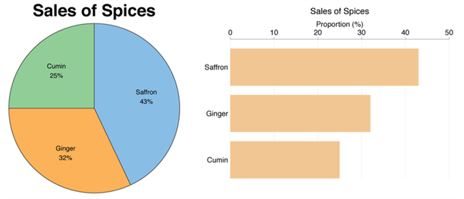
A pie chart (or a ‘donut chart’ if you stick a hole in the middle of it) is a circle divided into slices that show the relative sizes of data within a whole. If you’re using it to show percentages, make sure all the slices add up to 100%.

The pie chart is a familiar face at every party and is usually recognised by most people. However, one setback of using this method is our eyes sometimes can’t identify the differences in slices of a circle, and it’s nearly impossible to compare similar slices from two different pie charts, making them the villains in the eyes of data analysts.

Bonus example: A literal ‘pie’ chart! 🥧

The bar chart is a chart that presents a bunch of items from the same category, usually in the form of rectangular bars that are placed at an equal distance from each other. Their heights or lengths depict the values they represent.

They can be as simple as this:

Or more complex and detailed like this example of presentation of data. Contributing to an effective statistic presentation, this one is a grouped bar chart that not only allows you to compare categories but also the groups within them as well.

Similar in appearance to the bar chart but the rectangular bars in histograms don’t often have the gap like their counterparts.

Instead of measuring categories like weather preferences or favourite films as a bar chart does, a histogram only measures things that can be put into numbers.

Teachers can use presentation graphs like a histogram to see which score group most of the students fall into, like in this example above.

Recordings to ways of displaying data, we shouldn’t overlook the effectiveness of line graphs. Line graphs are represented by a group of data points joined together by a straight line. There can be one or more lines to compare how several related things change over time. 

On a line chart’s horizontal axis, you usually have text labels, dates or years, while the vertical axis usually represents the quantity (e.g.: budget, temperature or percentage).

A pictogram graph uses pictures or icons relating to the main topic to visualise a small dataset. The fun combination of colours and illustrations makes it a frequent use at schools.

Pictograms are a breath of fresh air if you want to stay away from the monotonous line chart or bar chart for a while. However, they can present a very limited amount of data and sometimes they are only there for displays and do not represent real statistics.

If presenting five or more variables in the form of a bar chart is too stuffy then you should try using a radar chart, which is one of the most creative ways to present data.

Radar charts show data in terms of how they compare to each other starting from the same point. Some also call them ‘spider charts’ because each aspect combined looks like a spider web.

Radar charts can be a great use for parents who’d like to compare their child’s grades with their peers to lower their self-esteem. You can see that each angular represents a subject with a score value ranging from 0 to 100. Each student’s score across 5 subjects is highlighted in a different colour.

If you think that this method of data presentation somehow feels familiar, then you’ve probably encountered one while playing Pokémon .

A heat map represents data density in colours. The bigger the number, the more colour intense that data will be represented.

Most U.S citizens would be familiar with this data presentation method in geography. For elections, many news outlets assign a specific colour code to a state, with blue representing one candidate and red representing the other. The shade of either blue or red in each state shows the strength of the overall vote in that state.

Another great thing you can use a heat map for is to map what visitors to your site click on. The more a particular section is clicked the ‘hotter’ the colour will turn, from blue to bright yellow to red.

If you present your data in dots instead of chunky bars, you’ll have a scatter plot. 

A scatter plot is a grid with several inputs showing the relationship between two variables. It’s good at collecting seemingly random data and revealing some telling trends.

For example, in this graph, each dot shows the average daily temperature versus the number of beach visitors across several days. You can see that the dots get higher as the temperature increases, so it’s likely that hotter weather leads to more visitors.

5 Data Presentation Mistakes to Avoid

#1 – assume your audience understands what the numbers represent.

You may know all the behind-the-scenes of your data since you’ve worked with them for weeks, but your audience doesn’t.

Showing without telling only invites more and more questions from your audience, as they have to constantly make sense of your data, wasting the time of both sides as a result.

While showing your data presentations, you should tell them what the data are about before hitting them with waves of numbers first. You can use interactive activities such as polls , word clouds , online quiz and Q&A sections , combined with icebreaker games , to assess their understanding of the data and address any confusion beforehand.

#2 – Use the wrong type of chart

Charts such as pie charts must have a total of 100% so if your numbers accumulate to 193% like this example below, you’re definitely doing it wrong.

Before making a chart, ask yourself: what do I want to accomplish with my data? Do you want to see the relationship between the data sets, show the up and down trends of your data, or see how segments of one thing make up a whole?

Remember, clarity always comes first. Some data visualisations may look cool, but if they don’t fit your data, steer clear of them. 

#3 – Make it 3D

3D is a fascinating graphical presentation example. The third dimension is cool, but full of risks.

Can you see what’s behind those red bars? Because we can’t either. You may think that 3D charts add more depth to the design, but they can create false perceptions as our eyes see 3D objects closer and bigger than they appear, not to mention they cannot be seen from multiple angles.

#4 – Use different types of charts to compare contents in the same category

This is like comparing a fish to a monkey. Your audience won’t be able to identify the differences and make an appropriate correlation between the two data sets. 

Next time, stick to one type of data presentation only. Avoid the temptation of trying various data visualisation methods in one go and make your data as accessible as possible.

#5 – Bombard the audience with too much information

The goal of data presentation is to make complex topics much easier to understand, and if you’re bringing too much information to the table, you’re missing the point.

The more information you give, the more time it will take for your audience to process it all. If you want to make your data understandable and give your audience a chance to remember it, keep the information within it to an absolute minimum. You should set your session with open-ended questions , to avoid dead-communication!

What are the Best Methods of Data Presentation?

Finally, which is the best way to present data?

The answer is…

There is none 😄 Each type of presentation has its own strengths and weaknesses and the one you choose greatly depends on what you’re trying to do. 

For example:

• Go for a scatter plot if you’re exploring the relationship between different data values, like seeing whether the sales of ice cream go up because of the temperature or because people are just getting more hungry and greedy each day?
• Go for a line graph if you want to mark a trend over time. 
• Go for a heat map if you like some fancy visualisation of the changes in a geographical location, or to see your visitors’ behaviour on your website.
• Go for a pie chart (especially in 3D) if you want to be shunned by others because it was never a good idea👇

What is chart presentation?

A chart presentation is a way of presenting data or information using visual aids such as charts, graphs, and diagrams. The purpose of a chart presentation is to make complex information more accessible and understandable for the audience.

When can I use charts for presentation?

Charts can be used to compare data, show trends over time, highlight patterns, and simplify complex information.

Why should use charts for presentation?

You should use charts to ensure your contents and visual look clean, as they are the visual representative, provide clarity, simplicity, comparison, contrast and super time-saving!

What are the 4 graphical methods of presenting data?

Histogram, Smoothed frequency graph, Pie diagram or Pie chart, Cumulative or ogive frequency graph, and Frequency Polygon.

Leah Nguyen

Words that convert, stories that stick. I turn complex ideas into engaging narratives - helping audiences learn, remember, and take action.

Tips to Engage with Polls & Trivia

More from AhaSlides

Data Collection, Presentation and Analysis

• First Online: 25 May 2023

Cite this chapter

• Uche M. Mbanaso 4 ,
• Lucienne Abrahams 5 &
• Kennedy Chinedu Okafor 6  

579 Accesses

This chapter covers the topics of data collection, data presentation and data analysis. It gives attention to data collection for studies based on experiments, on data derived from existing published or unpublished data sets, on observation, on simulation and digital twins, on surveys, on interviews and on focus group discussions. One of the interesting features of this chapter is the section dealing with using measurement scales in quantitative research, including nominal scales, ordinal scales, interval scales and ratio scales. It explains key facets of qualitative research including ethical clearance requirements. The chapter discusses the importance of data visualization as key to effective presentation of data, including tabular forms, graphical forms and visual charts such as those generated by Atlas.ti analytical software.

This is a preview of subscription content, log in via an institution to check access.

Access this chapter

• Available as EPUB and PDF
• Read on any device
• Instant download
• Own it forever
• Durable hardcover edition
• Dispatched in 3 to 5 business days
• Free shipping worldwide - see info

Tax calculation will be finalised at checkout

Purchases are for personal use only

Institutional subscriptions

Bibliography

Abdullah, M. F., & Ahmad, K. (2013). The mapping process of unstructured data to structured data. Proceedings of the 2013 International Conference on Research and Innovation in Information Systems (ICRIIS) , Malaysia , 151–155. https://doi.org/10.1109/ICRIIS.2013.6716700

Adnan, K., & Akbar, R. (2019). An analytical study of information extraction from unstructured and multidimensional big data. Journal of Big Data, 6 , 91. https://doi.org/10.1186/s40537-019-0254-8

Article   Google Scholar  

Alsheref, F. K., & Fattoh, I. E. (2020). Medical text annotation tool based on IBM Watson Platform. Proceedings of the 2020 6th international conference on advanced computing and communication systems (ICACCS) , India , 1312–1316. https://doi.org/10.1109/ICACCS48705.2020.9074309

Cinque, M., Cotroneo, D., Della Corte, R., & Pecchia, A. (2014). What logs should you look at when an application fails? Insights from an industrial case study. Proceedings of the 2014 44th Annual IEEE/IFIP International Conference on Dependable Systems and Networks , USA , 690–695. https://doi.org/10.1109/DSN.2014.69

Gideon, L. (Ed.). (2012). Handbook of survey methodology for the social sciences . Springer.

Google Scholar  

Leedy, P., & Ormrod, J. (2015). Practical research planning and design (12th ed.). Pearson Education.

Madaan, A., Wang, X., Hall, W., & Tiropanis, T. (2018). Observing data in IoT worlds: What and how to observe? In Living in the Internet of Things: Cybersecurity of the IoT – 2018 (pp. 1–7). https://doi.org/10.1049/cp.2018.0032

Chapter   Google Scholar  

Mahajan, P., & Naik, C. (2019). Development of integrated IoT and machine learning based data collection and analysis system for the effective prediction of agricultural residue/biomass availability to regenerate clean energy. Proceedings of the 2019 9th International Conference on Emerging Trends in Engineering and Technology – Signal and Information Processing (ICETET-SIP-19) , India , 1–5. https://doi.org/10.1109/ICETET-SIP-1946815.2019.9092156 .

Mahmud, M. S., Huang, J. Z., Salloum, S., Emara, T. Z., & Sadatdiynov, K. (2020). A survey of data partitioning and sampling methods to support big data analysis. Big Data Mining and Analytics, 3 (2), 85–101. https://doi.org/10.26599/BDMA.2019.9020015

Miswar, S., & Kurniawan, N. B. (2018). A systematic literature review on survey data collection system. Proceedings of the 2018 International Conference on Information Technology Systems and Innovation (ICITSI) , Indonesia , 177–181. https://doi.org/10.1109/ICITSI.2018.8696036

Mosina, C. (2020). Understanding the diffusion of the internet: Redesigning the global diffusion of the internet framework (Research report, Master of Arts in ICT Policy and Regulation). LINK Centre, University of the Witwatersrand. https://hdl.handle.net/10539/30723

Nkamisa, S. (2021). Investigating the integration of drone management systems to create an enabling remote piloted aircraft regulatory environment in South Africa (Research report, Master of Arts in ICT Policy and Regulation). LINK Centre, University of the Witwatersrand. https://hdl.handle.net/10539/33883

QuestionPro. (2020). Survey research: Definition, examples and methods . https://www.questionpro.com/article/survey-research.html

Rajanikanth, J. & Kanth, T. V. R. (2017). An explorative data analysis on Bangalore City Weather with hybrid data mining techniques using R. Proceedings of the 2017 International Conference on Current Trends in Computer, Electrical, Electronics and Communication (CTCEEC) , India , 1121-1125. https://doi/10.1109/CTCEEC.2017.8455008

Rao, R. (2003). From unstructured data to actionable intelligence. IT Professional, 5 , 29–35. https://www.researchgate.net/publication/3426648_From_Unstructured_Data_to_Actionable_Intelligence

Schulze, P. (2009). Design of the research instrument. In P. Schulze (Ed.), Balancing exploitation and exploration: Organizational antecedents and performance effects of innovation strategies (pp. 116–141). Gabler. https://doi.org/10.1007/978-3-8349-8397-8_6

Usanov, A. (2015). Assessing cybersecurity: A meta-analysis of threats, trends and responses to cyber attacks . The Hague Centre for Strategic Studies. https://www.researchgate.net/publication/319677972_Assessing_Cyber_Security_A_Meta-analysis_of_Threats_Trends_and_Responses_to_Cyber_Attacks

Van de Kaa, G., De Vries, H. J., van Heck, E., & van den Ende, J. (2007). The emergence of standards: A meta-analysis. Proceedings of the 2007 40th Annual Hawaii International Conference on Systems Science (HICSS’07) , USA , 173a–173a. https://doi.org/10.1109/HICSS.2007.529

Download references

Author information

Authors and affiliations.

Centre for Cybersecurity Studies, Nasarawa State University, Keffi, Nigeria

Uche M. Mbanaso

LINK Centre, University of the Witwatersrand, Johannesburg, South Africa

Lucienne Abrahams

Department of Mechatronics Engineering, Federal University of Technology, Owerri, Nigeria

Kennedy Chinedu Okafor

You can also search for this author in PubMed   Google Scholar

Rights and permissions

Reprints and permissions

Copyright information

© 2023 The Author(s), under exclusive license to Springer Nature Switzerland AG

About this chapter

Mbanaso, U.M., Abrahams, L., Okafor, K.C. (2023). Data Collection, Presentation and Analysis. In: Research Techniques for Computer Science, Information Systems and Cybersecurity. Springer, Cham. https://doi.org/10.1007/978-3-031-30031-8_7

Download citation

DOI : https://doi.org/10.1007/978-3-031-30031-8_7

Published : 25 May 2023

Publisher Name : Springer, Cham

Print ISBN : 978-3-031-30030-1

Online ISBN : 978-3-031-30031-8

eBook Packages : Engineering Engineering (R0)

Share this chapter

Anyone you share the following link with will be able to read this content:

Sorry, a shareable link is not currently available for this article.

Provided by the Springer Nature SharedIt content-sharing initiative

• Publish with us

Policies and ethics

• Find a journal
• Track your research

A .gov website belongs to an official government organization in the United States.

A lock ( ) or https:// means you've safely connected to the .gov website. Share sensitive information only on official, secure websites.

• Guidelines and Guidance Library
• Core Practices
• Isolation Precautions Guideline
• Disinfection and Sterilization Guideline
• Environmental Infection Control Guidelines
• Hand Hygiene Guidelines
• Multidrug-resistant Organisms (MDRO) Management Guidelines
• Catheter-Associated Urinary Tract Infections (CAUTI) Prevention Guideline
• Tools and resources
• Evaluating Environmental Cleaning

Infection Control Basics

• Infection control prevents or stops the spread of infections in healthcare settings.
• Healthcare workers can reduce the risk of healthcare-associated infections and protect themselves, patients and visitors by following CDC guidelines.

Germs are a part of everyday life. Germs live in our air, soil, water and in and on our bodies. Some germs are helpful, others are harmful.

An infection occurs when germs enter the body, increase in number and the body reacts. Only a small portion of germs can cause infection.

Terms to know

• Sources : places where infectious agents (germs) live (e.g., sinks, surfaces, human skin). Sources are also called reservoirs.
• Susceptible person: someone who is not vaccinated or otherwise immune. For example, a person with a weakened immune system who has a way for the germs to enter the body.
• Transmission: a way germs move to the susceptible person. Germs depend on people, the environment and/or medical equipment to move in healthcare settings. Transmission is also called a pathway.
• Colonization: when someone has germs on or in their body but does not have symptoms of an infection. Colonized people can still transmit the germs they carry.

For an infection to occur, germs must transmit to a person from a source, enter their body, invade tissues, multiply and cause a reaction.

How it works in healthcare settings

Sources can be:.

• People such as patients, healthcare workers and visitors.
• Dry surfaces in patient care areas such as bed rails, medical equipment, countertops and tables).
• Wet surfaces, moist environments and biofilms (collections of microorganisms that stick to each other and surfaces in moist environments, like the insides of pipes).
• Cooling towers, faucets and sinks, and equipment such as ventilators.
• Indwelling medical devices such as catheters and IV lines.
• Dust or decaying debris such as construction dust or wet materials from water leaks.

Transmission can happen through activities such as:

• Physical contact, like when a healthcare provider touches medical equipment that has germs on it and then touches a patient before cleaning their hands.
• Sprays and splashes when an infected person coughs or sneezes. This creates droplets containing the germs, and the droplets land on a person's eyes, nose or mouth.
• Inhalation when infected patients cough or talk, or construction zones kick up dirt and dust containing germs, which another person breathes in.
• Sharps injuries such as when someone is accidentally stuck with a used needle.

A person can become more susceptible to infection when:

• They have underlying medical conditions such as diabetes, cancer or organ transplantation. These can decrease the immune system's ability to fight infection.
• They take medications such as antibiotics, steroids and certain cancer fighting medications. These can decrease the body's ability to fight infection.
• They receive treatments or procedures such as urinary catheters, tubes and surgery, which can provide additional ways for germs to enter the body.

Recommendations

Healthcare providers.

Healthcare providers can perform basic infection prevention measures to prevent infection.

There are 2 tiers of recommended precautions to prevent the spread of infections in healthcare settings:

• Standard Precautions , used for all patient care.
• Transmission-based Precautions , used for patients who may be infected or colonized with certain germs.

There are also transmission- and germ-specific guidelines providers can follow to prevent transmission and healthcare-associated infections from happening.

Learn more about how to protect yourself from infections in healthcare settings.

For healthcare providers and settings

• Project Firstline : infection control education for all frontline healthcare workers.
• Infection prevention, control and response resources for outbreak investigations, the infection control assessment and response (ICAR) tool and more.
• Infection control specifically for surfaces and water management programs in healthcare settings.
• Preventing multi-drug resistant organisms (MDROs).

Infection Control

CDC provides information on infection control and clinical safety to help reduce the risk of infections among healthcare workers, patients, and visitors.

For Everyone

Health care providers, public health.

McKinsey Global Private Markets Review 2024: Private markets in a slower era

At a glance, macroeconomic challenges continued.

McKinsey Global Private Markets Review 2024: Private markets: A slower era

If 2022 was a tale of two halves, with robust fundraising and deal activity in the first six months followed by a slowdown in the second half, then 2023 might be considered a tale of one whole. Macroeconomic headwinds persisted throughout the year, with rising financing costs, and an uncertain growth outlook taking a toll on private markets. Full-year fundraising continued to decline from 2021’s lofty peak, weighed down by the “denominator effect” that persisted in part due to a less active deal market. Managers largely held onto assets to avoid selling in a lower-multiple environment, fueling an activity-dampening cycle in which distribution-starved limited partners (LPs) reined in new commitments.

About the authors

This article is a summary of a larger report, available as a PDF, that is a collaborative effort by Fredrik Dahlqvist , Alastair Green , Paul Maia, Alexandra Nee , David Quigley , Aditya Sanghvi , Connor Mangan, John Spivey, Rahel Schneider, and Brian Vickery , representing views from McKinsey’s Private Equity & Principal Investors Practice.

Performance in most private asset classes remained below historical averages for a second consecutive year. Decade-long tailwinds from low and falling interest rates and consistently expanding multiples seem to be things of the past. As private market managers look to boost performance in this new era of investing, a deeper focus on revenue growth and margin expansion will be needed now more than ever.

Perspectives on a slower era in private markets

Global fundraising contracted.

Fundraising fell 22 percent across private market asset classes globally to just over $1 trillion, as of year-end reported data—the lowest total since 2017. Fundraising in North America, a rare bright spot in 2022, declined in line with global totals, while in Europe, fundraising proved most resilient, falling just 3 percent. In Asia, fundraising fell precipitously and now sits 72 percent below the region’s 2018 peak.

Despite difficult fundraising conditions, headwinds did not affect all strategies or managers equally. Private equity (PE) buyout strategies posted their best fundraising year ever, and larger managers and vehicles also fared well, continuing the prior year’s trend toward greater fundraising concentration.

The numerator effect persisted

Despite a marked recovery in the denominator—the 1,000 largest US retirement funds grew 7 percent in the year ending September 2023, after falling 14 percent the prior year, for example 1 “U.S. retirement plans recover half of 2022 losses amid no-show recession,” Pensions and Investments , February 12, 2024. —many LPs remain overexposed to private markets relative to their target allocations. LPs started 2023 overweight: according to analysis from CEM Benchmarking, average allocations across PE, infrastructure, and real estate were at or above target allocations as of the beginning of the year. And the numerator grew throughout the year, as a lack of exits and rebounding valuations drove net asset values (NAVs) higher. While not all LPs strictly follow asset allocation targets, our analysis in partnership with global private markets firm StepStone Group suggests that an overallocation of just one percentage point can reduce planned commitments by as much as 10 to 12 percent per year for five years or more.

Despite these headwinds, recent surveys indicate that LPs remain broadly committed to private markets. In fact, the majority plan to maintain or increase allocations over the medium to long term.

Investors fled to known names and larger funds

Fundraising concentration reached its highest level in over a decade, as investors continued to shift new commitments in favor of the largest fund managers. The 25 most successful fundraisers collected 41 percent of aggregate commitments to closed-end funds (with the top five managers accounting for nearly half that total). Closed-end fundraising totals may understate the extent of concentration in the industry overall, as the largest managers also tend to be more successful in raising non-institutional capital.

While the largest funds grew even larger—the largest vehicles on record were raised in buyout, real estate, infrastructure, and private debt in 2023—smaller and newer funds struggled. Fewer than 1,700 funds of less than $1 billion were closed during the year, half as many as closed in 2022 and the fewest of any year since 2012. New manager formation also fell to the lowest level since 2012, with just 651 new firms launched in 2023.

Whether recent fundraising concentration and a spate of M&A activity signals the beginning of oft-rumored consolidation in the private markets remains uncertain, as a similar pattern developed in each of the last two fundraising downturns before giving way to renewed entrepreneurialism among general partners (GPs) and commitment diversification among LPs. Compared with how things played out in the last two downturns, perhaps this movie really is different, or perhaps we’re watching a trilogy reusing a familiar plotline.

Dry powder inventory spiked (again)

Private markets assets under management totaled $13.1 trillion as of June 30, 2023, and have grown nearly 20 percent per annum since 2018. Dry powder reserves—the amount of capital committed but not yet deployed—increased to $3.7 trillion, marking the ninth consecutive year of growth. Dry powder inventory—the amount of capital available to GPs expressed as a multiple of annual deployment—increased for the second consecutive year in PE, as new commitments continued to outpace deal activity. Inventory sat at 1.6 years in 2023, up markedly from the 0.9 years recorded at the end of 2021 but still within the historical range. NAV grew as well, largely driven by the reluctance of managers to exit positions and crystallize returns in a depressed multiple environment.

Private equity strategies diverged

Buyout and venture capital, the two largest PE sub-asset classes, charted wildly different courses over the past 18 months. Buyout notched its highest fundraising year ever in 2023, and its performance improved, with funds posting a (still paltry) 5 percent net internal rate of return through September 30. And although buyout deal volumes declined by 19 percent, 2023 was still the third-most-active year on record. In contrast, venture capital (VC) fundraising declined by nearly 60 percent, equaling its lowest total since 2015, and deal volume fell by 36 percent to the lowest level since 2019. VC funds returned –3 percent through September, posting negative returns for seven consecutive quarters. VC was the fastest-growing—as well as the highest-performing—PE strategy by a significant margin from 2010 to 2022, but investors appear to be reevaluating their approach in the current environment.

Private equity entry multiples contracted

PE buyout entry multiples declined by roughly one turn from 11.9 to 11.0 times EBITDA, slightly outpacing the decline in public market multiples (down from 12.1 to 11.3 times EBITDA), through the first nine months of 2023. For nearly a decade leading up to 2022, managers consistently sold assets into a higher-multiple environment than that in which they had bought those assets, providing a substantial performance tailwind for the industry. Nowhere has this been truer than in technology. After experiencing more than eight turns of multiple expansion from 2009 to 2021 (the most of any sector), technology multiples have declined by nearly three turns in the past two years, 50 percent more than in any other sector. Overall, roughly two-thirds of the total return for buyout deals that were entered in 2010 or later and exited in 2021 or before can be attributed to market multiple expansion and leverage. Now, with falling multiples and higher financing costs, revenue growth and margin expansion are taking center stage for GPs.

Real estate receded

Demand uncertainty, slowing rent growth, and elevated financing costs drove cap rates higher and made price discovery challenging, all of which weighed on deal volume, fundraising, and investment performance. Global closed-end fundraising declined 34 percent year over year, and funds returned −4 percent in the first nine months of the year, losing money for the first time since the 2007–08 global financial crisis. Capital shifted away from core and core-plus strategies as investors sought liquidity via redemptions in open-end vehicles, from which net outflows reached their highest level in at least two decades. Opportunistic strategies benefited from this shift, with investors focusing on capital appreciation over income generation in a market where alternative sources of yield have grown more attractive. Rising interest rates widened bid–ask spreads and impaired deal volume across food groups, including in what were formerly hot sectors: multifamily and industrial.

Private debt pays dividends

Debt again proved to be the most resilient private asset class against a turbulent market backdrop. Fundraising declined just 13 percent, largely driven by lower commitments to direct lending strategies, for which a slower PE deal environment has made capital deployment challenging. The asset class also posted the highest returns among all private asset classes through September 30. Many private debt securities are tied to floating rates, which enhance returns in a rising-rate environment. Thus far, managers appear to have successfully navigated the rising incidence of default and distress exhibited across the broader leveraged-lending market. Although direct lending deal volume declined from 2022, private lenders financed an all-time high 59 percent of leveraged buyout transactions last year and are now expanding into additional strategies to drive the next era of growth.

Infrastructure took a detour

After several years of robust growth and strong performance, infrastructure and natural resources fundraising declined by 53 percent to the lowest total since 2013. Supply-side timing is partially to blame: five of the seven largest infrastructure managers closed a flagship vehicle in 2021 or 2022, and none of those five held a final close last year. As in real estate, investors shied away from core and core-plus investments in a higher-yield environment. Yet there are reasons to believe infrastructure’s growth will bounce back. Limited partners (LPs) surveyed by McKinsey remain bullish on their deployment to the asset class, and at least a dozen vehicles targeting more than $10 billion were actively fundraising as of the end of 2023. Multiple recent acquisitions of large infrastructure GPs by global multi-asset-class managers also indicate marketwide conviction in the asset class’s potential.

Private markets still have work to do on diversity

Private markets firms are slowly improving their representation of females (up two percentage points over the prior year) and ethnic and racial minorities (up one percentage point). On some diversity metrics, including entry-level representation of women, private markets now compare favorably with corporate America. Yet broad-based parity remains elusive and too slow in the making. Ethnic, racial, and gender imbalances are particularly stark across more influential investing roles and senior positions. In fact, McKinsey’s research  reveals that at the current pace, it would take several decades for private markets firms to reach gender parity at senior levels. Increasing representation across all levels will require managers to take fresh approaches to hiring, retention, and promotion.

Artificial intelligence generating excitement

The transformative potential of generative AI was perhaps 2023’s hottest topic (beyond Taylor Swift). Private markets players are excited about the potential for the technology to optimize their approach to thesis generation, deal sourcing, investment due diligence, and portfolio performance, among other areas. While the technology is still nascent and few GPs can boast scaled implementations, pilot programs are already in flight across the industry, particularly within portfolio companies. Adoption seems nearly certain to accelerate throughout 2024.

Private markets in a slower era

If private markets investors entered 2023 hoping for a return to the heady days of 2021, they likely left the year disappointed. Many of the headwinds that emerged in the latter half of 2022 persisted throughout the year, pressuring fundraising, dealmaking, and performance. Inflation moderated somewhat over the course of the year but remained stubbornly elevated by recent historical standards. Interest rates started high and rose higher, increasing the cost of financing. A reinvigorated public equity market recovered most of 2022’s losses but did little to resolve the valuation uncertainty private market investors have faced for the past 18 months.

Within private markets, the denominator effect remained in play, despite the public market recovery, as the numerator continued to expand. An activity-dampening cycle emerged: higher cost of capital and lower multiples limited the ability or willingness of general partners (GPs) to exit positions; fewer exits, coupled with continuing capital calls, pushed LP allocations higher, thereby limiting their ability or willingness to make new commitments. These conditions weighed on managers’ ability to fundraise. Based on data reported as of year-end 2023, private markets fundraising fell 22 percent from the prior year to just over $1 trillion, the largest such drop since 2009 (Exhibit 1).

The impact of the fundraising environment was not felt equally among GPs. Continuing a trend that emerged in 2022, and consistent with prior downturns in fundraising, LPs favored larger vehicles and the scaled GPs that typically manage them. Smaller and newer managers struggled, and the number of sub–$1 billion vehicles and new firm launches each declined to its lowest level in more than a decade.

Despite the decline in fundraising, private markets assets under management (AUM) continued to grow, increasing 12 percent to $13.1 trillion as of June 30, 2023. 2023 fundraising was still the sixth-highest annual haul on record, pushing dry powder higher, while the slowdown in deal making limited distributions.

Investment performance across private market asset classes fell short of historical averages. Private equity (PE) got back in the black but generated the lowest annual performance in the past 15 years, excluding 2022. Closed-end real estate produced negative returns for the first time since 2009, as capitalization (cap) rates expanded across sectors and rent growth dissipated in formerly hot sectors, including multifamily and industrial. The performance of infrastructure funds was less than half of its long-term average and even further below the double-digit returns generated in 2021 and 2022. Private debt was the standout performer (if there was one), outperforming all other private asset classes and illustrating the asset class’s countercyclical appeal.

Private equity down but not out

Higher financing costs, lower multiples, and an uncertain macroeconomic environment created a challenging backdrop for private equity managers in 2023. Fundraising declined for the second year in a row, falling 15 percent to $649 billion, as LPs grappled with the denominator effect and a slowdown in distributions. Managers were on the fundraising trail longer to raise this capital: funds that closed in 2023 were open for a record-high average of 20.1 months, notably longer than 18.7 months in 2022 and 14.1 months in 2018. VC and growth equity strategies led the decline, dropping to their lowest level of cumulative capital raised since 2015. Fundraising in Asia fell for the fourth year of the last five, with the greatest decline in China.

Despite the difficult fundraising context, a subset of strategies and managers prevailed. Buyout managers collectively had their best fundraising year on record, raising more than $400 billion. Fundraising in Europe surged by more than 50 percent, resulting in the region’s biggest haul ever. The largest managers raised an outsized share of the total for a second consecutive year, making 2023 the most concentrated fundraising year of the last decade (Exhibit 2).

Despite the drop in aggregate fundraising, PE assets under management increased 8 percent to $8.2 trillion. Only a small part of this growth was performance driven: PE funds produced a net IRR of just 2.5 percent through September 30, 2023. Buyouts and growth equity generated positive returns, while VC lost money. PE performance, dating back to the beginning of 2022, remains negative, highlighting the difficulty of generating attractive investment returns in a higher interest rate and lower multiple environment. As PE managers devise value creation strategies to improve performance, their focus includes ensuring operating efficiency and profitability of their portfolio companies.

Deal activity volume and count fell sharply, by 21 percent and 24 percent, respectively, which continued the slower pace set in the second half of 2022. Sponsors largely opted to hold assets longer rather than lock in underwhelming returns. While higher financing costs and valuation mismatches weighed on overall deal activity, certain types of M&A gained share. Add-on deals, for example, accounted for a record 46 percent of total buyout deal volume last year.

Real estate recedes

For real estate, 2023 was a year of transition, characterized by a litany of new and familiar challenges. Pandemic-driven demand issues continued, while elevated financing costs, expanding cap rates, and valuation uncertainty weighed on commercial real estate deal volumes, fundraising, and investment performance.

Managers faced one of the toughest fundraising environments in many years. Global closed-end fundraising declined 34 percent to $125 billion. While fundraising challenges were widespread, they were not ubiquitous across strategies. Dollars continued to shift to large, multi-asset class platforms, with the top five managers accounting for 37 percent of aggregate closed-end real estate fundraising. In April, the largest real estate fund ever raised closed on a record $30 billion.

Capital shifted away from core and core-plus strategies as investors sought liquidity through redemptions in open-end vehicles and reduced gross contributions to the lowest level since 2009. Opportunistic strategies benefited from this shift, as investors turned their attention toward capital appreciation over income generation in a market where alternative sources of yield have grown more attractive.

In the United States, for instance, open-end funds, as represented by the National Council of Real Estate Investment Fiduciaries Fund Index—Open-End Equity (NFI-OE), recorded $13 billion in net outflows in 2023, reversing the trend of positive net inflows throughout the 2010s. The negative flows mainly reflected $9 billion in core outflows, with core-plus funds accounting for the remaining outflows, which reversed a 20-year run of net inflows.

As a result, the NAV in US open-end funds fell roughly 16 percent year over year. Meanwhile, global assets under management in closed-end funds reached a new peak of $1.7 trillion as of June 2023, growing 14 percent between June 2022 and June 2023.

Real estate underperformed historical averages in 2023, as previously high-performing multifamily and industrial sectors joined office in producing negative returns caused by slowing demand growth and cap rate expansion. Closed-end funds generated a pooled net IRR of −3.5 percent in the first nine months of 2023, losing money for the first time since the global financial crisis. The lone bright spot among major sectors was hospitality, which—thanks to a rush of postpandemic travel—returned 10.3 percent in 2023. 2 Based on NCREIFs NPI index. Hotels represent 1 percent of total properties in the index. As a whole, the average pooled lifetime net IRRs for closed-end real estate funds from 2011–20 vintages remained around historical levels (9.8 percent).

Global deal volume declined 47 percent in 2023 to reach a ten-year low of $650 billion, driven by widening bid–ask spreads amid valuation uncertainty and higher costs of financing (Exhibit 3). 3 CBRE, Real Capital Analytics Deal flow in the office sector remained depressed, partly as a result of continued uncertainty in the demand for space in a hybrid working world.

During a turbulent year for private markets, private debt was a relative bright spot, topping private markets asset classes in terms of fundraising growth, AUM growth, and performance.

Fundraising for private debt declined just 13 percent year over year, nearly ten percentage points less than the private markets overall. Despite the decline in fundraising, AUM surged 27 percent to $1.7 trillion. And private debt posted the highest investment returns of any private asset class through the first three quarters of 2023.

Private debt’s risk/return characteristics are well suited to the current environment. With interest rates at their highest in more than a decade, current yields in the asset class have grown more attractive on both an absolute and relative basis, particularly if higher rates sustain and put downward pressure on equity returns (Exhibit 4). The built-in security derived from debt’s privileged position in the capital structure, moreover, appeals to investors that are wary of market volatility and valuation uncertainty.

Direct lending continued to be the largest strategy in 2023, with fundraising for the mostly-senior-debt strategy accounting for almost half of the asset class’s total haul (despite declining from the previous year). Separately, mezzanine debt fundraising hit a new high, thanks to the closings of three of the largest funds ever raised in the strategy.

Over the longer term, growth in private debt has largely been driven by institutional investors rotating out of traditional fixed income in favor of private alternatives. Despite this growth in commitments, LPs remain underweight in this asset class relative to their targets. In fact, the allocation gap has only grown wider in recent years, a sharp contrast to other private asset classes, for which LPs’ current allocations exceed their targets on average. According to data from CEM Benchmarking, the private debt allocation gap now stands at 1.4 percent, which means that, in aggregate, investors must commit hundreds of billions in net new capital to the asset class just to reach current targets.

Private debt was not completely immune to the macroeconomic conditions last year, however. Fundraising declined for the second consecutive year and now sits 23 percent below 2021’s peak. Furthermore, though private lenders took share in 2023 from other capital sources, overall deal volumes also declined for the second year in a row. The drop was largely driven by a less active PE deal environment: private debt is predominantly used to finance PE-backed companies, though managers are increasingly diversifying their origination capabilities to include a broad new range of companies and asset types.

Infrastructure and natural resources take a detour

For infrastructure and natural resources fundraising, 2023 was an exceptionally challenging year. Aggregate capital raised declined 53 percent year over year to $82 billion, the lowest annual total since 2013. The size of the drop is particularly surprising in light of infrastructure’s recent momentum. The asset class had set fundraising records in four of the previous five years, and infrastructure is often considered an attractive investment in uncertain markets.

While there is little doubt that the broader fundraising headwinds discussed elsewhere in this report affected infrastructure and natural resources fundraising last year, dynamics specific to the asset class were at play as well. One issue was supply-side timing: nine of the ten largest infrastructure GPs did not close a flagship fund in 2023. Second was the migration of investor dollars away from core and core-plus investments, which have historically accounted for the bulk of infrastructure fundraising, in a higher rate environment.

The asset class had some notable bright spots last year. Fundraising for higher-returning opportunistic strategies more than doubled the prior year’s total (Exhibit 5). AUM grew 18 percent, reaching a new high of $1.5 trillion. Infrastructure funds returned a net IRR of 3.4 percent in 2023; this was below historical averages but still the second-best return among private asset classes. And as was the case in other asset classes, investors concentrated commitments in larger funds and managers in 2023, including in the largest infrastructure fund ever raised.

The outlook for the asset class, moreover, remains positive. Funds targeting a record amount of capital were in the market at year-end, providing a robust foundation for fundraising in 2024 and 2025. A recent spate of infrastructure GP acquisitions signal multi-asset managers’ long-term conviction in the asset class, despite short-term headwinds. Global megatrends like decarbonization and digitization, as well as revolutions in energy and mobility, have spurred new infrastructure investment opportunities around the world, particularly for value-oriented investors that are willing to take on more risk.

Private markets make measured progress in DEI

Diversity, equity, and inclusion (DEI) has become an important part of the fundraising, talent, and investing landscape for private market participants. Encouragingly, incremental progress has been made in recent years, including more diverse talent being brought to entry-level positions, investing roles, and investment committees. The scope of DEI metrics provided to institutional investors during fundraising has also increased in recent years: more than half of PE firms now provide data across investing teams, portfolio company boards, and portfolio company management (versus investment team data only). 4 “ The state of diversity in global private markets: 2023 ,” McKinsey, August 22, 2023.

In 2023, McKinsey surveyed 66 global private markets firms that collectively employ more than 60,000 people for the second annual State of diversity in global private markets report. 5 “ The state of diversity in global private markets: 2023 ,” McKinsey, August 22, 2023. The research offers insight into the representation of women and ethnic and racial minorities in private investing as of year-end 2022. In this chapter, we discuss where the numbers stand and how firms can bring a more diverse set of perspectives to the table.

The statistics indicate signs of modest advancement. Overall representation of women in private markets increased two percentage points to 35 percent, and ethnic and racial minorities increased one percentage point to 30 percent (Exhibit 6). Entry-level positions have nearly reached gender parity, with female representation at 48 percent. The share of women holding C-suite roles globally increased 3 percentage points, while the share of people from ethnic and racial minorities in investment committees increased 9 percentage points. There is growing evidence that external hiring is gradually helping close the diversity gap, especially at senior levels. For example, 33 percent of external hires at the managing director level were ethnic or racial minorities, higher than their existing representation level (19 percent).

Yet, the scope of the challenge remains substantial. Women and minorities continue to be underrepresented in senior positions and investing roles. They also experience uneven rates of progress due to lower promotion and higher attrition rates, particularly at smaller firms. Firms are also navigating an increasingly polarized workplace today, with additional scrutiny and a growing number of lawsuits against corporate diversity and inclusion programs, particularly in the US, which threatens to impact the industry’s pace of progress.

Fredrik Dahlqvist is a senior partner in McKinsey’s Stockholm office; Alastair Green  is a senior partner in the Washington, DC, office, where Paul Maia and Alexandra Nee  are partners; David Quigley  is a senior partner in the New York office, where Connor Mangan is an associate partner and Aditya Sanghvi  is a senior partner; Rahel Schneider is an associate partner in the Bay Area office; John Spivey is a partner in the Charlotte office; and Brian Vickery  is a partner in the Boston office.

The authors wish to thank Jonathan Christy, Louis Dufau, Vaibhav Gujral, Graham Healy-Day, Laura Johnson, Ryan Luby, Tripp Norton, Alastair Rami, Henri Torbey, and Alex Wolkomir for their contributions

The authors would also like to thank CEM Benchmarking and the StepStone Group for their partnership in this year's report.

This article was edited by Arshiya Khullar, an editor in the Gurugram office.

Explore a career with us

Related articles.

CEO alpha: A new approach to generating private equity outperformance

Private equity turns to resiliency strategies for software investments

The state of diversity in global private markets: 2022