types of hypothesis testing in six sigma

Six Sigma Study Guide

Study notes and guides for Six Sigma certification tests

Hypothesis Testing Overview

Posted by Ted Hessing

You may know all the statistics in the world, but if you jump straight from those statistics to the wrong conclusion, you could make a million-dollar error. That’s where hypothesis testing comes in. It combines tried-and-tested analysis tools, real-world data, and a framework that allows us to test our assumptions and beliefs. This way, we can say how likely something is to be true or not within a given standard of accuracy.

When using hypothesis testing, we create the following:

• A null hypothesis (H0): the assumption that the experimental results are due to chance alone; nothing (from 6M) influenced our results.
• An alternative hypothesis (Ha):  we expect to find a particular outcome.

These hypotheses should always be mutually exclusive: if one is true, the other is false.

Once we have our null and alternative hypotheses, we evaluate them with a sample of an entire population, check our results, and conclude based on those results.

Note: We never accept a NULL hypothesis; we simply fail to reject it. We are always testing the NULL.

Basic Testing Process

The basic testing process consists of five steps:

• Identify the question
• Determine the significance
• Choose the test
• Interpret the results
• Make a decision.

Read more about the hypothesis testing process .

Terminology

This field uses a lot of specialist terminologies. We’ve collated a list of the most common terms and their meanings for easy lookup. See the hypothesis testing terminology list .

Tailed Hypothesis Tests

These tests are commonly referred to according to their ‘tails’ or the critical regions that exist within them. There are three basic types: right-tailed, left-tailed, and two-tailed. Read more about tailed hypothesis tests .

Errors in Hypothesis Testing

When discussing an error in this context, the word has a very specific meaning: it refers to incorrectly either rejecting or accepting a hypothesis. Read more about errors in hypothesis testing .

We use P-values to determine how statistically significant our test results are and how probable we’ll make an error. Read more about p-values .

Types of Hypothesis Tests

One aspect of testing that can confuse the new student is finding which–out of many available tests–is correct to use.

Parametric Tests

You can use these tests when it’s implied that a distribution is assumed for the population or the data is a sample from a distribution (often a normal distribution ).

Non Parametric Tests

You use non-parametric tests when you don’t know, can’t assume, and can’t identify what kind of distribution you have.

Hypothesis Test Study Guide

We run through the types of tests and briefly explain what each one is commonly used for. Read more about types of hypothesis tests .

Significance of Central Limit Theorem

The Central Limit Theorem is important for inferential statistics because it allows us to safely assume that the sampling distribution of the mean will be normal in most cases. This means that we can take advantage of statistical techniques that assume a normal distribution.

The Central Limit Theorem is one of the most profound and useful statistical and probability results. The large samples (more than 30) from any sort of distribution of the sample means will follow a  normal distribution . The central limit theorem is vital in statistics for two main reasons—the normality assumption and the precision of the estimates.

The spread of the sample means is less (narrower) than the spread of the population you’re sampling from. So, it does not matter how the original population is skewed.

• The means of the sampling distribution of the mean is equal to the population mean µ x̅  =µ X
• The standard deviation of the sample means equals the standard deviation of the population divided by the square root of the sample size: σ( x̅ ) = σ(x) / √(n)

Central Limit Theorem allows using confidence intervals, hypothesis testing, DOE, regression analysis, and other analytical techniques. Many statistics have approximately normal distributions for large sample sizes, even when we are sampling from a non-normal distribution.

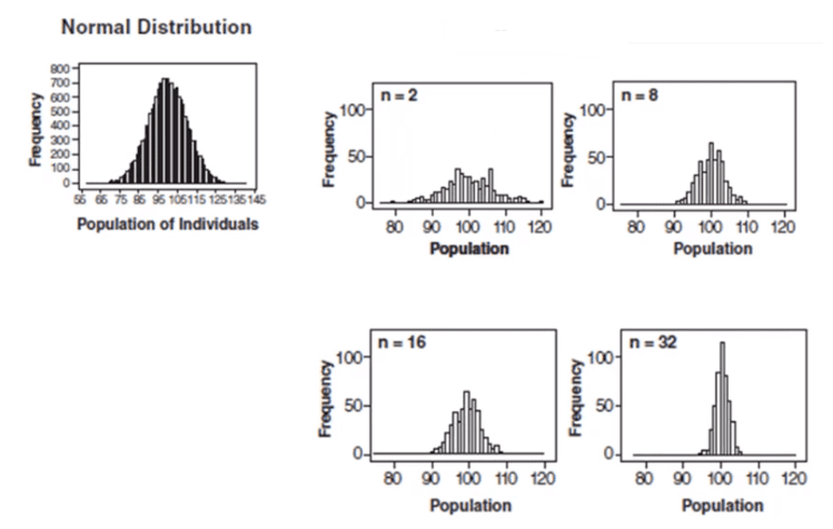
Control charts and the central limit theorem

In the above graph, subgroup sizes of 2, 8, 16, and 32 were used in this analysis. We can see the impact of the subgrouping. In Figure 2 (n=8), the histogram is not as wide and looks more “normally” distributed than Figure 1. Figure 3 shows the histogram for subgroup averages when n = 16, it is even more narrow and it looks more normally distributed. Figures 1 through 4 show, that as n increases, the distribution becomes narrower and more bell-shaped -just as the central limit theorem says. This means that we can often use well-developed statistical inference procedures and probability calculations that are based on a normal distribution, even if we are sampling from a population that is not normal, provided we have a large sample size.

Overview Videos

Leave a Reply Cancel reply

Your email address will not be published. Required fields are marked *

This site uses Akismet to reduce spam. Learn how your comment data is processed .

Insert/edit link

Enter the destination URL

Or link to existing content

🚀 Chart your career path in cutting-edge domains.

Talk to a career counsellor for personalised guidance 🤝.

9 Types of Hypothesis Testing for Six Sigma Data Analysis

Table of content, hypothesis testing and steps involved in it, why is hypothesis testing needed in six sigma, benefits of using hypothesis testing in six sigma, how to choose a hypothesis test for six sigma data analysis.

Hypothesis testing is a statistical technique that tells us whether the tests of our experiment have shown any meaningful results. After hypothesis testing, you can tell whether the test results have happened due to pure chance or a significant intervention. If it is down to chances, it will be difficult or impossible to replicate the results. However, if it is due to a particular instance, knowledge of that will enable us to replicate the results time and again.

Source:   Medium

In hypothesis testing steps, the person conducting the test states these two hypotheses. Since both are opposites, only one of the two hypotheses can be correct. The alpha and beta risks are also identified as a part of this statistical data analysis. Alpha risk is the risk of incorrectly rejecting the null hypothesis. Beta risk, on the other hand, is the risk of not rejecting an incorrect null hypothesis. 

The next step is to formulate the plan to evaluate the available data to arrive at the correct hypothesis. The tester carries out the plan and analyzes the sample. The tester then summarizes the result from the data analysis tools to find out which of the two hypotheses stands. Based on the data, the tester may reject the null hypothesis or the testing may fail to reject it. This, in short, answers   what hypothesis testing is.

Using statistical techniques and formulae is a part of a Six Sigma manager’s work profile. In a Six Sigma project, the manager makes key decisions based on statistical test inferences. Hypothesis testing allows a greater degree of confidence in these decisions because they are not merely the mathematical differences between two samples.

Let us assume that a Six Sigma project produces thermal power. The quality of coal used as a raw material may influence the wattage of power generated. As the Six Sigma project manager, you want to establish whether there is a statistically significant relationship between the coal grade used and the power generated. With hypothesis testing, you can frame the proper null hypothesis, identify the alpha risk and the beta risk, and calculate the test statistic or p-value. This will help you to arrive at a more informed conclusion on your coal quality and power generation theory.

Hypothesis testing is useful in   measuring the progress of your project   as you strive to improve your product or service. Since it’s a test of significance, hypothesis testing helps you prove whether the data is statistically significant. In terms of Six Sigma hypothesis testing examples, it could be decisive in spotting the improvements in your product or service or the lack of them. 

In a decision made based on a sample study, there is a probability that non-representative samples may flaw the decision. However, a hypothesis test converts a practical problem into a statistical problem, consequently giving us an estimate of the probability of a non-representative sample. 

A process may face problems with centering or problems with spread. In other words, the mean of two processes may be different, or the variances of the two processes may be different. Both are instances of differences in distribution. Hypothesis testing can help us analyze whether the difference between the two data sets is statistically significant.

1) Normality –   Normality tests whether the sample distributes normally. Here the null hypothesis states that the population is normally distributed, while the alternative hypothesis states otherwise. If the p-value of the test is less than the defined significance level, the tester can reject the null hypothesis. 

The sample size is crucial in normality testing. If the sample size is large, a small deviation can project a statistically significant p-value, which will be difficult to detect in case of a small sample size. A Six Sigma project manager would consider the sample size before relying on the normality test result. 

2) T-test –   A T-test compares the respective means of two data groups. In a project, it is useful to find out whether two data sets are different from one another or whether a process or treatment has an effect on the population. In a T-test, the data has to be independent and normally distributed to an aggregable degree. The data groups should have a similar amount of variance. These assumptions are part of the T-test as it is a parametric test of difference. T-tests will make the pairwise comparison only, and other types of hypothesis testing are for more than two groups.

4) Homogeneity of Variance (HOV) –   HOV tests the homogeneity of variances between populations. With an assumption that variances among different groups are equal, you can pool such groups together to estimate the population variance. With HOV you get a better assurance of this variance homogeneity, which can encourage you to use smaller sample sizes or make better interpretations from the same sample size. 

In the case of two groups, you can assume that the variance would be one (the null hypothesis). Anything other than a variance of one, i.e., equal, would be in support of the alternative hypothesis. In the case of three or more populations, the alternative hypothesis would be that one population variance is different.

5) Analysis of Variance (ANOVA) –   ANOVA compares the means of different groups to test if they significantly vary from one another. For instance, in a project, ANOVA can check whether there are multiple approaches to solving a particular problem. The mean, in this case, time taken to solve the problem, of all these approaches will help us find out the effectiveness of each approach. If there are only two groups, T-test and ANOVA will show the same result. The null hypothesis in ANOVA is that no sample means have any significant difference. Any difference in even one sample means would mean rejection of the null hypothesis.

6) Mood’s Median –   Mood’s Median tests the similarity of medians across two or more populations. It is a non-parametric test, which means that it doesn’t make any assumption based on normally distributed data, unlike ANOVA, for instance. Non-parametric tests are a better failsafe against wrong inferences. Nevertheless, it has a null hypothesis as it should, which is that there are no significant differences between the medians under consideration.

7) Welch’s T-test –   Also known as Welch’s Test for Unequal Variances, it checks two sample means for significant differences. The null hypothesis is that the means are equal while the alternative hypothesis is that the means are not equal. In Welch’s test, there is a modification in the degrees of freedom over the student’s T-test. Unlike the T-test, it doesn’t assume equal variances. It is more reliable when both the groups have unequal sample sizes and variances. But statisticians don’t recommend Welch’s T-test for small sample sizes. 

8) Kruskal-Wallis H Test –   Like Mood’s Median, Kruskal-Wallis H Test is a non-parametric variation of ANOVA. The two hypotheses in it are that the population medians are or are not equal. To run this test, the tester uses ranks of the data value, rather than the data values themselves. While Kruskal-Wallis will find out the significant differences between the populations, it doesn’t tell you which groups are, in fact, different. This test assumes there is one independent variable with two or more levels. The observations should be independent, with no relation among data points in different groups. Besides, all the tested groups must have s\distributions of similar shape.   

9) Box-Cox Power Transformation –   Box-Cox Power Transformation allows a broader test diameter, with normality not being a required assumption. It is known as power transformation because it transforms non-normal dependent variables into a normal shape. Box-Cox Power transformation uses an exponent called lambda. Its test value can vary from -5 to 5. Of all the test values of the lambda, the one that’s optimal value has the best approximation of a normal distribution curve.

As can be seen in the different types of hypothesis testing, the purpose of most of these tests are different, or should we say – significantly different. Even in the case of tests that are similar in mechanism and technique, smaller differences are there, whether it’s in the assumptions or the inclusion of an additional element.

Therefore, if you want to compare a population mean with a given standard, or two different population means, a T-test is the test to use. On the other hand, if means of more than two populations need comparing, Six Sigma project managers often use the ANOVA test.

If you are doing a comparison among the variances of two or more populations, the HOV is one of the appropriate tests. On the other hand, comparing the medians of two or more populations can be appropriate for the Mood’s Median test. To compare the differences in output between two or more sub-groups, a Chi-Square Test of Independence is the way to go. 

The choice of the hypothesis depends on the   needs of the Six Sigma data analytics. The broader goal in Six Sigma remains that we have to move the process mean and restrict the standard deviation to a minimum. The decisions are based on sample data because of the cost-effectiveness, rather than an exhaustive study of the total population. Hypothesis testing enables Six Sigma teams to decide whether there are different population parameters, or the difference, if any, is due to sample variations. 

Once the Six Sigma team understands the problem it can correlate the practical difference in outcomes with the statistical differences found in testing. The hypothesis testing identifies the difference. The selection of the test type, in turn, will depend on underlying factors. Is the difference a change in the mean or the variance, for instance?

Planning to become a skilled Data Analyst? Learn Data Science from scratch with OdinSchool's Data Science Course and get dedicated placement assistance!

About the Author

Meet Raktim Sharma, a talented writer who enjoys baking and taking pictures in addition to contributing insightful articles. He contributes a plethora of knowledge to our blog with years of experience and skill.

Related Posts

Career Transition with Data Science Upskill Amidst Many Challenges!

A journey filled with twists and turns, Waquar Ahmed's career path unfolded like a novel, each chapter a step...

Unlocking Success: AON Analyst's Middle-Class Climb to a 124% Salary Hike!

Discover the importance of structured learning in the pursuit of success in the data science field.

The Role of Machine Learning in Data Science

Data Science is a field that studies data and employs a series of methods, algorithms, systems, and tools to...

Join OdinSchool's Data Science Bootcamp

With job assistance.

• Guide: Hypothesis Testing

Daniel Croft

Daniel Croft is an experienced continuous improvement manager with a Lean Six Sigma Black Belt and a Bachelor's degree in Business Management. With more than ten years of experience applying his skills across various industries, Daniel specializes in optimizing processes and improving efficiency. His approach combines practical experience with a deep understanding of business fundamentals to drive meaningful change.

• Last Updated: September 8, 2023
• Learn Lean Sigma

In the world of data-driven decision-making, Hypothesis Testing stands as a cornerstone methodology. It serves as the statistical backbone for a multitude of sectors, from manufacturing and logistics to healthcare and finance. But what exactly is Hypothesis Testing, and why is it so indispensable? Simply put, it’s a technique that allows you to validate or invalidate claims about a population based on sample data. Whether you’re looking to streamline a manufacturing process, optimize logistics, or improve customer satisfaction, Hypothesis Testing offers a structured approach to reach conclusive, data-supported decisions.

The graphical example above provides a simplified snapshot of a hypothesis test. The bell curve represents a normal distribution, the green area is where you’d accept the null hypothesis ( H 0​), and the red area is the “rejection zone,” where you’d favor the alternative hypothesis ( Ha ​). The vertical blue line represents the threshold value or “critical value,” beyond which you’d reject H 0​.

Here’s a graphical example of a hypothesis test, which you can include in the introduction section of your guide. In this graph:

• The curve represents a standard normal distribution, often encountered in hypothesis tests.
• The green-shaded area signifies the “Acceptance Region,” where you would fail to reject the null hypothesis ( H 0​).
• The red-shaded areas are the “Rejection Regions,” where you would reject H 0​ in favor of the alternative hypothesis ( Ha ​).
• The blue dashed lines indicate the “Critical Values” (±1.96), which are the thresholds for rejecting H 0​.

This graphical representation serves as a conceptual foundation for understanding the mechanics of hypothesis testing. It visually illustrates what it means to accept or reject a hypothesis based on a predefined level of significance.

Table of Contents

What is hypothesis testing.

Hypothesis testing is a structured procedure in statistics used for drawing conclusions about a larger population based on a subset of that population, known as a sample. The method is widely used across different industries and sectors for a variety of purposes. Below, we’ll dissect the key components of hypothesis testing to provide a more in-depth understanding.

The Hypotheses: H 0 and Ha

In every hypothesis test, there are two competing statements:

• Null Hypothesis ( H 0) : This is the “status quo” hypothesis that you are trying to test against. It is a statement that asserts that there is no effect or difference. For example, in a manufacturing setting, the null hypothesis might state that a new production process does not improve the average output quality.
• Alternative Hypothesis ( Ha or H 1) : This is what you aim to prove by conducting the hypothesis test. It is the statement that there is an effect or difference. Using the same manufacturing example, the alternative hypothesis might state that the new process does improve the average output quality.

Significance Level ( α )

Before conducting the test, you decide on a “Significance Level” ( α ), typically set at 0.05 or 5%. This level represents the probability of rejecting the null hypothesis when it is actually true. Lower α values make the test more stringent, reducing the chances of a ‘false positive’.

Data Collection

You then proceed to gather data, which is usually a sample from a larger population. The quality of your test heavily relies on how well this sample represents the population. The data can be collected through various means such as surveys, observations, or experiments.

Statistical Test

Depending on the nature of the data and what you’re trying to prove, different statistical tests can be applied (e.g., t-test, chi-square test , ANOVA , etc.). These tests will compute a test statistic (e.g., t , 2 χ 2, F , etc.) based on your sample data.

Here are graphical examples of the distributions commonly used in three different types of statistical tests: t-test, Chi-square test, and ANOVA (Analysis of Variance), displayed side by side for comparison.

• Graph 1 (Leftmost): This graph represents a t-distribution, often used in t-tests. The t-distribution is similar to the normal distribution but tends to have heavier tails. It is commonly used when the sample size is small or the population variance is unknown.

Chi-square Test

• Graph 2 (Middle): The Chi-square distribution is used in Chi-square tests, often for testing independence or goodness-of-fit. Unlike the t-distribution, the Chi-square distribution is not symmetrical and only takes on positive values.

ANOVA (F-distribution)

• Graph 3 (Rightmost): The F-distribution is used in Analysis of Variance (ANOVA), a statistical test used to analyze the differences between group means. Like the Chi-square distribution, the F-distribution is also not symmetrical and takes only positive values.

These visual representations provide an intuitive understanding of the different statistical tests and their underlying distributions. Knowing which test to use and when is crucial for conducting accurate and meaningful hypothesis tests.

Decision Making

The test statistic is then compared to a critical value determined by the significance level ( α ) and the sample size. This comparison will give you a p-value. If the p-value is less than α , you reject the null hypothesis in favor of the alternative hypothesis. Otherwise, you fail to reject the null hypothesis.

Interpretation

Finally, you interpret the results in the context of what you were investigating. Rejecting the null hypothesis might mean implementing a new process or strategy, while failing to reject it might lead to a continuation of current practices.

To sum it up, hypothesis testing is not just a set of formulas but a methodical approach to problem-solving and decision-making based on data. It’s a crucial tool for anyone interested in deriving meaningful insights from data to make informed decisions.

Why is Hypothesis Testing Important?

Hypothesis testing is a cornerstone of statistical and empirical research, serving multiple functions in various fields. Let’s delve into each of the key areas where hypothesis testing holds significant importance:

Data-Driven Decisions

In today’s complex business environment, making decisions based on gut feeling or intuition is not enough; you need data to back up your choices. Hypothesis testing serves as a rigorous methodology for making decisions based on data. By setting up a null hypothesis and an alternative hypothesis, you can use statistical methods to determine which is more likely to be true given a data sample. This structured approach eliminates guesswork and adds empirical weight to your decisions, thereby increasing their credibility and effectiveness.

Risk Management

Hypothesis testing allows you to assign a ‘p-value’ to your findings, which is essentially the probability of observing the given sample data if the null hypothesis is true. This p-value can be directly used to quantify risk. For instance, a p-value of 0.05 implies there’s a 5% risk of rejecting the null hypothesis when it’s actually true. This is invaluable in scenarios like product launches or changes in operational processes, where understanding the risk involved can be as crucial as the decision itself.

Here’s an example to help you understand the concept better.

The graph above serves as a graphical representation to help explain the concept of a ‘p-value’ and its role in quantifying risk in hypothesis testing. Here’s how to interpret the graph:

Elements of the Graph

• The curve represents a Standard Normal Distribution , which is often used to represent z-scores in hypothesis testing.
• The red-shaded area on the right represents the Rejection Region . It corresponds to a 5% risk ( α =0.05) of rejecting the null hypothesis when it is actually true. This is the area where, if your test statistic falls, you would reject the null hypothesis.
• The green-shaded area represents the Acceptance Region , with a 95% level of confidence. If your test statistic falls in this region, you would fail to reject the null hypothesis.
• The blue dashed line is the Critical Value (approximately 1.645 in this example). If your standardized test statistic (z-value) exceeds this point, you enter the rejection region, and your p-value becomes less than 0.05, leading you to reject the null hypothesis.

Relating to Risk Management

The p-value can be directly related to risk management. For example, if you’re considering implementing a new manufacturing process, the p-value quantifies the risk of that decision. A low p-value (less than α ) would mean that the risk of rejecting the null hypothesis (i.e., going ahead with the new process) when it’s actually true is low, thus indicating a lower risk in implementing the change.

Quality Control

In sectors like manufacturing, automotive, and logistics, maintaining a high level of quality is not just an option but a necessity. Hypothesis testing is often employed in quality assurance and control processes to test whether a certain process or product conforms to standards. For example, if a car manufacturing line claims its error rate is below 5%, hypothesis testing can confirm or disprove this claim based on a sample of products. This ensures that quality is not compromised and that stakeholders can trust the end product.

Resource Optimization

Resource allocation is a significant challenge for any organization. Hypothesis testing can be a valuable tool in determining where resources will be most effectively utilized. For instance, in a manufacturing setting, you might want to test whether a new piece of machinery significantly increases production speed. A hypothesis test could provide the statistical evidence needed to decide whether investing in more of such machinery would be a wise use of resources.

In the realm of research and development, hypothesis testing can be a game-changer. When developing a new product or process, you’ll likely have various theories or hypotheses. Hypothesis testing allows you to systematically test these, filtering out the less likely options and focusing on the most promising ones. This not only speeds up the innovation process but also makes it more cost-effective by reducing the likelihood of investing in ideas that are statistically unlikely to be successful.

In summary, hypothesis testing is a versatile tool that adds rigor, reduces risk, and enhances the decision-making and innovation processes across various sectors and functions.

This graphical representation makes it easier to grasp how the p-value is used to quantify the risk involved in making a decision based on a hypothesis test.

Step-by-Step Guide to Hypothesis Testing

To make this guide practical and helpful if you are new learning about the concept we will explain each step of the process and follow it up with an example of the method being applied to a manufacturing line, and you want to test if a new process reduces the average time it takes to assemble a product.

Step 1: State the Hypotheses

The first and foremost step in hypothesis testing is to clearly define your hypotheses. This sets the stage for your entire test and guides the subsequent steps, from data collection to decision-making. At this stage, you formulate two competing hypotheses:

Null Hypothesis ( H 0)

The null hypothesis is a statement that there is no effect or no difference, and it serves as the hypothesis that you are trying to test against. It’s the default assumption that any kind of effect or difference you suspect is not real, and is due to chance. Formulating a clear null hypothesis is crucial, as your statistical tests will be aimed at challenging this hypothesis.

In a manufacturing context, if you’re testing whether a new assembly line process has reduced the time it takes to produce an item, your null hypothesis ( H 0) could be:

H 0:”The new process does not reduce the average assembly time.”

Alternative Hypothesis ( Ha or H 1)

The alternative hypothesis is what you want to prove. It is a statement that there is an effect or difference. This hypothesis is considered only after you find enough evidence against the null hypothesis.

Continuing with the manufacturing example, the alternative hypothesis ( Ha ) could be:

Ha :”The new process reduces the average assembly time.”

Types of Alternative Hypothesis

Depending on what exactly you are trying to prove, the alternative hypothesis can be:

• Two-Sided : You’re interested in deviations in either direction (greater or smaller).
• One-Sided : You’re interested in deviations only in one direction (either greater or smaller).

Scenario: Reducing Assembly Time in a Car Manufacturing Plant

You are a continuous improvement manager at a car manufacturing plant. One of the assembly lines has been struggling with longer assembly times, affecting the overall production schedule. A new assembly process has been proposed, promising to reduce the assembly time per car. Before rolling it out on the entire line, you decide to conduct a hypothesis test to see if the new process actually makes a difference. Null Hypothesis ( H 0​) In this context, the null hypothesis would be the status quo, asserting that the new assembly process doesn’t reduce the assembly time per car. Mathematically, you could state it as: H 0:The average assembly time per car with the new process ≥ The average assembly time per car with the old process. Or simply: H 0​:”The new process does not reduce the average assembly time per car.” Alternative Hypothesis ( Ha ​ or H 1​) The alternative hypothesis is what you aim to prove — that the new process is more efficient. Mathematically, it could be stated as: Ha :The average assembly time per car with the new process < The average assembly time per car with the old process Or simply: Ha ​:”The new process reduces the average assembly time per car.” Types of Alternative Hypothesis In this example, you’re only interested in knowing if the new process reduces the time, making it a One-Sided Alternative Hypothesis .

Step 2: Determine the Significance Level ( α )

Once you’ve clearly stated your null and alternative hypotheses, the next step is to decide on the significance level, often denoted by α . The significance level is a threshold below which the null hypothesis will be rejected. It quantifies the level of risk you’re willing to accept when making a decision based on the hypothesis test.

What is a Significance Level?

The significance level, usually expressed as a percentage, represents the probability of rejecting the null hypothesis when it is actually true. Common choices for α are 0.05, 0.01, and 0.10, representing 5%, 1%, and 10% levels of significance, respectively.

• 5% Significance Level ( α =0.05) : This is the most commonly used level and implies that you are willing to accept a 5% chance of rejecting the null hypothesis when it is true.
• 1% Significance Level ( α =0.01) : This is a more stringent level, used when you want to be more sure of your decision. The risk of falsely rejecting the null hypothesis is reduced to 1%.
• 10% Significance Level ( α =0.10) : This is a more lenient level, used when you are willing to take a higher risk. Here, the chance of falsely rejecting the null hypothesis is 10%.

Continuing with the manufacturing example, let’s say you decide to set α =0.05, meaning you’re willing to take a 5% risk of concluding that the new process is effective when it might not be.

How to Choose the Right Significance Level?

Choosing the right significance level depends on the context and the consequences of making a wrong decision. Here are some factors to consider:

• Criticality of Decision : For highly critical decisions with severe consequences if wrong, a lower α like 0.01 may be appropriate.
• Resource Constraints : If the cost of collecting more data is high, you may choose a higher α to make a decision based on a smaller sample size.
• Industry Standards : Sometimes, the choice of α may be dictated by industry norms or regulatory guidelines.

By the end of Step 2, you should have a well-defined significance level that will guide the rest of your hypothesis testing process. This level serves as the cut-off for determining whether the observed effect or difference in your sample is statistically significant or not.

Continuing the Scenario: Reducing Assembly Time in a Car Manufacturing Plant

After formulating the hypotheses, the next step is to set the significance level ( α ) that will be used to interpret the results of the hypothesis test. This is a critical decision as it quantifies the level of risk you’re willing to accept when making a conclusion based on the test. Setting the Significance Level Given that assembly time is a critical factor affecting the production schedule, and ultimately, the company’s bottom line, you decide to be fairly stringent in your test. You opt for a commonly used significance level: α = 0.05 This means you are willing to accept a 5% chance of rejecting the null hypothesis when it is actually true. In practical terms, if you find that the p-value of the test is less than 0.05, you will conclude that the new process significantly reduces assembly time and consider implementing it across the entire line. Why α = 0.05 ? Industry Standard : A 5% significance level is widely accepted in many industries, including manufacturing, for hypothesis testing. Risk Management : By setting  α = 0.05 , you’re limiting the risk of concluding that the new process is effective when it may not be to just 5%. Balanced Approach : This level offers a balance between being too lenient (e.g., α=0.10) and too stringent (e.g., α=0.01), making it a reasonable choice for this scenario.

Step 3: Collect and Prepare the Data

After stating your hypotheses and setting the significance level, the next vital step is data collection. The data you collect serves as the basis for your hypothesis test, so it’s essential to gather accurate and relevant data.

Types of Data

Depending on your hypothesis, you’ll need to collect either:

• Quantitative Data : Numerical data that can be measured. Examples include height, weight, and temperature.
• Qualitative Data : Categorical data that represent characteristics. Examples include colors, gender, and material types.

Data Collection Methods

Various methods can be used to collect data, such as:

• Surveys and Questionnaires : Useful for collecting qualitative data and opinions.
• Observation : Collecting data through direct or participant observation.
• Experiments : Especially useful in scientific research where control over variables is possible.
• Existing Data : Utilizing databases, records, or any other data previously collected.

Sample Size

The sample size ( n ) is another crucial factor. A larger sample size generally gives more accurate results, but it’s often constrained by resources like time and money. The choice of sample size might also depend on the statistical test you plan to use.

Continuing with the manufacturing example, suppose you decide to collect data on the assembly time of 30 randomly chosen products, 15 made using the old process and 15 made using the new process. Here, your sample size n =30.

Data Preparation

Once data is collected, it often needs to be cleaned and prepared for analysis. This could involve:

• Removing Outliers : Outliers can skew the results and provide an inaccurate picture.
• Data Transformation : Converting data into a format suitable for statistical analysis.
• Data Coding : Categorizing or labeling data, necessary for qualitative data.

By the end of Step 3, you should have a dataset that is ready for statistical analysis. This dataset should be representative of the population you’re interested in and prepared in a way that makes it suitable for hypothesis testing.

With the hypotheses stated and the significance level set, you’re now ready to collect the data that will serve as the foundation for your hypothesis test. Given that you’re testing a change in a manufacturing process, the data will most likely be quantitative, representing the assembly time of cars produced on the line. Data Collection Plan You decide to use a Random Sampling Method for your data collection. For two weeks, assembly times for randomly selected cars will be recorded: one week using the old process and another week using the new process. Your aim is to collect data for 40 cars from each process, giving you a sample size ( n ) of 80 cars in total. Types of Data Quantitative Data : In this case, you’re collecting numerical data representing the assembly time in minutes for each car. Data Preparation Data Cleaning : Once the data is collected, you’ll need to inspect it for any anomalies or outliers that could skew your results. For example, if a significant machine breakdown happened during one of the weeks, you may need to adjust your data or collect more. Data Transformation : Given that you’re dealing with time, you may not need to transform your data, but it’s something to consider, depending on the statistical test you plan to use. Data Coding : Since you’re dealing with quantitative data in this scenario, coding is likely unnecessary unless you’re planning to categorize assembly times into bins (e.g., ‘fast’, ‘medium’, ‘slow’) for some reason. Example Data Points: Car_ID Process_Type Assembly_Time_Minutes 1 Old 38.53 2 Old 35.80 3 Old 36.96 4 Old 39.48 5 Old 38.74 6 Old 33.05 7 Old 36.90 8 Old 34.70 9 Old 34.79 … … … The complete dataset would contain 80 rows: 40 for the old process and 40 for the new process.

Step 4: Conduct the Statistical Test

After you have your hypotheses, significance level, and collected data, the next step is to actually perform the statistical test. This step involves calculations that will lead to a test statistic, which you’ll then use to make your decision regarding the null hypothesis.

Choose the Right Test

The first task is to decide which statistical test to use. The choice depends on several factors:

• Type of Data : Quantitative or Qualitative
• Sample Size : Large or Small
• Number of Groups or Categories : One-sample, Two-sample, or Multiple groups

For instance, you might choose a t-test for comparing means of two groups when you have a small sample size. Chi-square tests are often used for categorical data, and ANOVA is used for comparing means across more than two groups.

Calculation of Test Statistic

Once you’ve chosen the appropriate statistical test, the next step is to calculate the test statistic. This involves using the sample data in a specific formula for the chosen test.

Obtain the p-value

After calculating the test statistic, the next step is to find the p-value associated with it. The p-value represents the probability of observing the given test statistic if the null hypothesis is true.

• A small p-value (< α ) indicates strong evidence against the null hypothesis, so you reject the null hypothesis.
• A large p-value (> α ) indicates weak evidence against the null hypothesis, so you fail to reject the null hypothesis.

Make the Decision

You now compare the p-value to the predetermined significance level ( α ):

• If p < α , you reject the null hypothesis in favor of the alternative hypothesis.
• If p > α , you fail to reject the null hypothesis.

In the manufacturing case, if your calculated p-value is 0.03 and your α is 0.05, you would reject the null hypothesis, concluding that the new process effectively reduces the average assembly time.

By the end of Step 4, you will have either rejected or failed to reject the null hypothesis, providing a statistical basis for your decision-making process.

Now that you have collected and prepared your data, the next step is to conduct the actual statistical test to evaluate the null and alternative hypotheses. In this case, you’ll be comparing the mean assembly times between cars produced using the old and new processes to determine if the new process is statistically significantly faster. Choosing the Right Test Given that you have two sets of independent samples (old process and new process), a Two-sample t-test for Equality of Means seems appropriate for comparing the average assembly times. Preparing Data for Minitab Firstly, you would prepare your data in an Excel sheet or CSV file with one column for the assembly times using the old process and another column for the assembly times using the new process. Import this file into Minitab. Steps to Perform the Two-sample t-test in Minitab Open Minitab : Launch the Minitab software on your computer. Import Data : Navigate to File > Open and import your data file. Navigate to the t-test Menu : Go to Stat > Basic Statistics > 2-Sample t... . Select Columns : In the dialog box, specify the columns corresponding to the old and new process assembly times under “Sample 1” and “Sample 2.” Options : Click on Options and make sure that you set the confidence level to 95% (which corresponds to α = 0.05 ). Run the Test : Click OK to run the test. In this example output, the p-value is 0.0012, which is less than the significance level α = 0.05 . Hence, you would reject the null hypothesis. The t-statistic is -3.45, indicating that the mean of the new process is statistically significantly less than the mean of the old process, which aligns with your alternative hypothesis. Showing the data displayed as a Box plot in the below graphic it is easy to see the new process is statistically significantly better.

Why do a Hypothesis test?

You might ask, after all this why do a hypothesis test and not just look at the averages, which is a good question. While looking at average times might give you a general idea of which process is faster, hypothesis testing provides several advantages that a simple comparison of averages doesn’t offer:

Statistical Significance

Account for Random Variability : Hypothesis testing considers not just the averages, but also the variability within each group. This allows you to make more robust conclusions that account for random chance.

Quantify the Evidence : With hypothesis testing, you obtain a p-value that quantifies the strength of the evidence against the null hypothesis. A simple comparison of averages doesn’t provide this level of detail.

Control Type I Error : Hypothesis testing allows you to control the probability of making a Type I error (i.e., rejecting a true null hypothesis). This is particularly useful in settings where the consequences of such an error could be costly or risky.

Quantify Risk : Hypothesis testing provides a structured way to make decisions based on a predefined level of risk (the significance level, α ).

Decision-making Confidence

Objective Decision Making : The formal structure of hypothesis testing provides an objective framework for decision-making. This is especially useful in a business setting where decisions often have to be justified to stakeholders.

Replicability : The statistical rigor ensures that the results are replicable. Another team could perform the same test and expect to get similar results, which is not necessarily the case when comparing only averages.

Additional Insights

Understanding of Variability : Hypothesis testing often involves looking at measures of spread and distribution, not just the mean. This can offer additional insights into the processes you’re comparing.

Basis for Further Analysis : Once you’ve performed a hypothesis test, you can often follow it up with other analyses (like confidence intervals for the difference in means, or effect size calculations) that offer more detailed information.

In summary, while comparing averages is quicker and simpler, hypothesis testing provides a more reliable, nuanced, and objective basis for making data-driven decisions.

Step 5: Interpret the Results and Make Conclusions

Having conducted the statistical test and obtained the p-value, you’re now at a stage where you can interpret these results in the context of the problem you’re investigating. This step is crucial for transforming the statistical findings into actionable insights.

Interpret the p-value

The p-value you obtained tells you the significance of your results:

• Low p-value ( p < α ) : Indicates that the results are statistically significant, and it’s unlikely that the observed effects are due to random chance. In this case, you generally reject the null hypothesis.
• High p-value ( p > α ) : Indicates that the results are not statistically significant, and the observed effects could well be due to random chance. Here, you generally fail to reject the null hypothesis.

Relate to Real-world Context

You should then relate these statistical conclusions to the real-world context of your problem. This is where your expertise in your specific field comes into play.

In our manufacturing example, if you’ve found a statistically significant reduction in assembly time with a p-value of 0.03 (which is less than the α level of 0.05), you can confidently conclude that the new manufacturing process is more efficient. You might then consider implementing this new process across the entire assembly line.

Make Recommendations

Based on your conclusions, you can make recommendations for action or further study. For example:

• Implement Changes : If the test results are significant, consider making the changes on a larger scale.
• Further Research : If the test results are not clear or not significant, you may recommend further studies or data collection.
• Review Methodology : If you find that the results are not as expected, it might be useful to review the methodology and see if the test was conducted under the right conditions and with the right test parameters.

Document the Findings

Lastly, it’s essential to document all the steps taken, the methodology used, the data collected, and the conclusions drawn. This documentation is not only useful for any further studies but also for auditing purposes or for stakeholders who may need to understand the process and the findings.

By the end of Step 5, you’ll have turned the raw statistical findings into meaningful conclusions and actionable insights. This is the final step in the hypothesis testing process, making it a complete, robust method for informed decision-making.

You’ve successfully conducted the hypothesis test and found strong evidence to reject the null hypothesis in favor of the alternative: The new assembly process is statistically significantly faster than the old one. It’s now time to interpret these results in the context of your business operations and make actionable recommendations. Interpretation of Results Statistical Significance : The p-value of 0.0012 is well below the significance level of = 0.05   α = 0.05 , indicating that the results are statistically significant. Practical Significance : The boxplot and t-statistic (-3.45) suggest not just statistical, but also practical significance. The new process appears to be both consistently and substantially faster. Risk Assessment : The low p-value allows you to reject the null hypothesis with a high degree of confidence, meaning the risk of making a Type I error is minimal. Business Implications Increased Productivity : Implementing the new process could lead to an increase in the number of cars produced, thereby enhancing productivity. Cost Savings : Faster assembly time likely translates to lower labor costs. Quality Control : Consider monitoring the quality of cars produced under the new process closely to ensure that the speedier assembly does not compromise quality. Recommendations Implement New Process : Given the statistical and practical significance of the findings, recommend implementing the new process across the entire assembly line. Monitor and Adjust : Implement a control phase where the new process is monitored for both speed and quality. This could involve additional hypothesis tests or control charts. Communicate Findings : Share the results and recommendations with stakeholders through a formal presentation or report, emphasizing both the statistical rigor and the potential business benefits. Review Resource Allocation : Given the likely increase in productivity, assess if resources like labor and parts need to be reallocated to optimize the workflow further.

By following this step-by-step guide, you’ve journeyed through the rigorous yet enlightening process of hypothesis testing. From stating clear hypotheses to interpreting the results, each step has paved the way for making informed, data-driven decisions that can significantly impact your projects, business, or research.

Hypothesis testing is more than just a set of formulas or calculations; it’s a holistic approach to problem-solving that incorporates context, statistics, and strategic decision-making. While the process may seem daunting at first, each step serves a crucial role in ensuring that your conclusions are both statistically sound and practically relevant.

• McKenzie, C.R., 2004. Hypothesis testing and evaluation .  Blackwell handbook of judgment and decision making , pp.200-219.
• Park, H.M., 2015. Hypothesis testing and statistical power of a test.
• Eberhardt, L.L., 2003. What should we do about hypothesis testing? .  The Journal of wildlife management , pp.241-247.

Q: What is hypothesis testing in the context of Lean Six Sigma?

A: Hypothesis testing is a statistical method used in Lean Six Sigma to determine whether there is enough evidence in a sample of data to infer that a certain condition holds true for the entire population. In the Lean Six Sigma process, it’s commonly used to validate the effectiveness of process improvements by comparing performance metrics before and after changes are implemented. A null hypothesis ( H 0 ​ ) usually represents no change or effect, while the alternative hypothesis ( H 1 ​ ) indicates a significant change or effect.

Q: How do I determine which statistical test to use for my hypothesis?

A: The choice of statistical test for hypothesis testing depends on several factors, including the type of data (nominal, ordinal, interval, or ratio), the sample size, the number of samples (one sample, two samples, paired), and whether the data distribution is normal. For example, a t-test is used for comparing the means of two groups when the data is normally distributed, while a Chi-square test is suitable for categorical data to test the relationship between two variables. It’s important to choose the right test to ensure the validity of your hypothesis testing results.

Q: What is a p-value, and how does it relate to hypothesis testing?

A: A p-value is a probability value that helps you determine the significance of your results in hypothesis testing. It represents the likelihood of obtaining a result at least as extreme as the one observed during the test, assuming that the null hypothesis is true. In hypothesis testing, if the p-value is lower than the predetermined significance level (commonly α = 0.05 ), you reject the null hypothesis, suggesting that the observed effect is statistically significant. If the p-value is higher, you fail to reject the null hypothesis, indicating that there is not enough evidence to support the alternative hypothesis.

Q: Can you explain Type I and Type II errors in hypothesis testing?

A: Type I and Type II errors are potential errors that can occur in hypothesis testing. A Type I error, also known as a “false positive,” occurs when the null hypothesis is true, but it is incorrectly rejected. It is equivalent to a false alarm. On the other hand, a Type II error, or a “false negative,” happens when the null hypothesis is false, but it is erroneously failed to be rejected. This means a real effect or difference was missed. The risk of a Type I error is represented by the significance level ( α ), while the risk of a Type II error is denoted by β . Minimizing these errors is crucial for the reliability of hypothesis tests in continuous improvement projects.

Daniel Croft is a seasoned continuous improvement manager with a Black Belt in Lean Six Sigma. With over 10 years of real-world application experience across diverse sectors, Daniel has a passion for optimizing processes and fostering a culture of efficiency. He's not just a practitioner but also an avid learner, constantly seeking to expand his knowledge. Outside of his professional life, Daniel has a keen Investing, statistics and knowledge-sharing, which led him to create the website learnleansigma.com, a platform dedicated to Lean Six Sigma and process improvement insights.

Free Lean Six Sigma Templates

Improve your Lean Six Sigma projects with our free templates. They're designed to make implementation and management easier, helping you achieve better results.

Other Guides

• Certified Six Sigma Green Belt (CSSGB™)
• Certified Six Sigma Black Belt (CSSBB™)
• Certified Six Sigma Master Black Belt (CSSMBB™)
• Certified Six Sigma Champion (CSSC™)
• Certified Six Sigma Deployment Leader (CSSDL™)
• Certified Six Sigma Yellow Belt (CSSYB™)
• Certified Six Sigma Trainer (CSSTRA™)
• Certified Six Sigma Coach (CSSCOA™)
• Register Your Six Sigma Certification Program
• International Scrum Institute™
• International DevOps Certification Academy™
• International Organization for Project Management (IO4PM™)
• International Software Test Institute™
• International MBA Institute™
• Your Blog (US Army Personnel Selected Six Sigma Institute™)
• Our Industry Review and Feedback
• Our Official Recognition and Industry Clients
• Our Corporate Partners Program
• Frequently Asked Questions (FAQ)
• Shareable Digital Badge And Six Sigma Certifications Validation Registry (NEW)
• Recommend International Six Sigma Institute™ To Friends
• Introducing: World's First & Only Six Sigma AI Assistant (NEW)
• Your Free Six Sigma Book
• Your Free Premium Six Sigma Training
• Your Sample Six Sigma Certification Test Questions
• Your Free Six Sigma Events
• Terms and Conditions
• Privacy Policy

Six Sigma Hypothesis Testing: Results with P-Value & Data

Hypothesis testing is crucial in Six Sigma as it provides a statistical framework to analyze process improvements, measure project progress, and make data-driven decisions. By using hypothesis testing, Six Sigma practitioners can effectively determine whether changes made to a process have resulted in meaningful improvements or not, thus ensuring strategic decision-making based on evidence.

Six Sigma DMAIC - Analyze Phase - Hypothesis Testing

What is the difference that can be detected using Hypothesis Testing?

• Step 1: Determine appropriate Hypothesis test
• Step 2: State the Null Hypothesis Ho and Alternate Hypothesis Ha
• Step 3: Calculate Test Statistics / P-value against table value of test statistic
• Step 4: Interpret results – Accept or reject Ho
• Ho = Null Hypothesis – There is No statistically significant difference between the two groups
• Ha = Alternate Hypothesis – There is statistically significant difference between the two groups

P Value – Also known as Probability value, it is a statistical measure which indicates the probability of making an α error. The value ranges between 0 and 1. We normally work with 5% alpha risk, a p value lower than 0.05 means that we reject the Null hypothesis and accept alternate hypothesis.

What is P-Value in Six Sigma?

Six sigma hypothesis: null and alternative.

It's crucial to understand that both hypotheses play complementary roles in hypothesis testing. While the null hypothesis anchors the current state or standard processes, the alternative hypothesis serves as a beacon for evaluating potential enhancements or variances resulting from process improvements or changes. When these two hypotheses are utilized effectively, they provide a structured framework for detailed analysis and decision-making.

Tools for Six Sigma Hypothesis Testing

Difference analysis in six sigma hypothesis testing.

Applying a t-test for comparing means or another suitable hypothesis testing method will help evaluate whether the decrease from 10 minutes to 8 minutes is meaningful or just due to chance. It allows decision-makers to make informed choices based on statistical test inferences rather than relying solely on anecdotal evidence or individual perceptions.

Deciding Hypothesis Validity in Six Sigma

This decision-making process plays a pivotal role in organizational decision-making because it guides leaders in determining whether observed changes are truly beneficial or merely due to chance. In essence, what we are doing here is looking for hard evidence through data analysis—evidence that supports our belief about positive changes resulting from specific actions taken within our processes.

Enhancing Precision via Reduction of Variation

Practical applications of hypothesis testing in six sigma.

All these scenarios underscore the practical relevance of hypothesis testing in enabling organizations to make informed decisions and allocate resources effectively based on tangible evidence rather than intuition or assumptions.

Frequently Asked Questions about Six Sigma Hypothesis Testing

What are some common types of hypothesis tests used in six sigma projects, how does hypothesis testing fit into the six sigma methodology, how do you determine the significance level and power of a hypothesis test in six sigma, what are some practical examples or case studies where hypothesis testing has been applied successfully in a six sigma project.

What are the key steps involved in conducting hypothesis testing in Six Sigma?

What is the purpose of hypothesis testing in six sigma, in the dmaic method, which stage identifies with the confirmation and testing the statistical solution, project y is continuous and x is discrete to validate variance between subgroups. what does this mean, which hypothesis test will you perform when the y is continuous normal and x is discrete. what does this this mean, what is sigma test, what is beta testing is six sigma, what null hypothesis in six sigma, recap of six sigma hypothesis testing with p-values.

Mastering Six Sigma hypothesis testing, including the interpretation of P-values, is a skill that can significantly enhance one's ability to drive process improvements and minimize variation. The recap of these testing techniques serves as a valuable reminder of the precision required in decision-making within the Six Sigma framework. Whether you're initiating a project or refining existing processes, the insights gained from comprehending P-values contribute to the success of your continuous improvement initiatives.

Your Six Sigma Training Table of Contents

We guarantee that your free online training will make you pass your six sigma certification exam.

THE ONLY BOOK. YOU CAN SIMPLY LEARN SIX SIGMA.

YOUR SIX SIGMA REVEALED 2ND EDITION IS NOW READY. CLICK BOOK COVER FOR FREE DOWNLOAD...

Hypothesis Testing

Hypothesis Testing in Lean Six Sigma

One of the essential tools in the Lean Six Sigma toolkit is hypothesis testing. Hypothesis testing is crucial in the Define-Measure-Analyze-Improve-Control (DMAIC) cycle, helping organizations make data-driven decisions and achieve continuous improvement. This article will explore the significance of hypothesis testing in Lean Six Sigma, its key concepts, and practical applications.

Understanding Hypothesis Testing

Hypothesis testing is a statistical method used to determine whether there is a significant difference between two or more sets of data. In the context of Lean Six Sigma, it is primarily used to assess the impact of process changes or improvements. The process of hypothesis testing involves formulating two competing hypotheses:

• Null Hypothesis (H0):   This hypothesis assumes that there is no significant difference or effect. It represents the status quo or the current state of the process.
• Alternative Hypothesis (Ha) or (H1):   This hypothesis suggests that there is a significant difference or effect resulting from process changes or improvements.

The goal of hypothesis testing is to collect and analyze data to either accept or reject the null hypothesis in favor of the alternative hypothesis.

Key Steps in Hypothesis Testing in Lean Six Sigma

• Define the Problem: The first step in Lean Six Sigma’s DMAIC cycle is clearly defining the problem. This involves understanding the process, identifying the problem’s scope, and setting measurable goals for improvement.
• Formulate Hypotheses: Once the problem is defined, the next step is to formulate the null and alternative hypotheses. This step is crucial as it sets the foundation for the hypothesis testing process.
• Collect Data: Data collection is critical to hypothesis testing. Lean Six Sigma practitioners gather relevant data using various methods, ensuring the data is accurate, representative, and sufficient for analysis.
• Analyze Data: Statistical analysis is the heart of hypothesis testing. Different statistical tests are used depending on the data type and the analysis objectives. Common tests include t-tests, chi-square tests, and analysis of variance (ANOVA) .
• Determine Significance Level: A significance level (alpha) is set to determine the threshold for accepting or rejecting the null hypothesis in hypothesis testing. Common significance levels are 0.05 and 0.01, representing a 5% and 1% chance of making a Type I error, respectively.
• Calculate Test Statistic: The test statistic is computed from the collected data and compared to a critical value or a p-value to determine its significance.
• Make a Decision: Based on the test statistic and significance level, a decision is made either to reject the null hypothesis in favor of the alternative hypothesis or to fail to reject the null hypothesis.
• Draw Conclusions: The final step involves drawing conclusions based on the decision made in step 7. These conclusions inform the next steps in the Lean Six Sigma DMAIC cycle, whether it be process improvement, optimization, or control.

Practical Applications of Hypothesis Testing in Lean Six Sigma

• Process Improvement: Hypothesis testing is often used to assess whether process improvements, such as changes in machinery, materials, or procedures, lead to significant enhancements in process performance.
• Root Cause Analysis: Lean Six Sigma practitioners employ hypothesis testing to identify the root causes of process defects or variations, helping organizations address the underlying issues effectively.
• Product Quality Control: Manufacturers use hypothesis testing to ensure the quality of products meets predefined standards and specifications, reducing defects and customer complaints.
• Cost Reduction: By testing hypotheses related to cost reduction initiatives, organizations can determine whether cost-saving measures are effective and sustainable.
• Customer Satisfaction: Hypothesis testing can be applied to customer feedback data to determine if changes in products or services result in increased customer satisfaction.

Six Sigma Green Belt vs Six Sigma Black Belt in Hypothesis Testing

Six Sigma Black Belts and Six Sigma Green Belts both use hypothesis testing as a critical tool in process improvement projects, but there are differences in their roles and responsibilities, which influence how they employ hypothesis testing:

1. Project Leadership and Complexity:

• Black Belts : Black Belts typically lead larger and more complex improvement projects. They are responsible for selecting projects that significantly impact the organization’s strategic goals. Hypothesis testing for Black Belts often involves multifaceted analyses, intricate data collection strategies, and a deeper understanding of statistical techniques.
• Green Belts : Green Belts usually work on smaller-scale projects or support Black Belts on larger projects. Their projects may have a narrower focus and involve less complex hypothesis testing than Black Belts.

2. Statistical Expertise:

• Black Belts : Black Belts are expected to have a higher level of statistical expertise. They are often skilled in advanced statistical methods and can handle complex data analysis. They might use more advanced statistical techniques such as multivariate analysis, design of experiments (DOE), or regression modeling.
• Green Belts : Green Belts have a solid understanding of basic statistical methods and hypothesis testing but may not have the same depth of expertise as Black Belts. They typically use simpler statistical tools for hypothesis testing.

3. Project Oversight and Coaching:

• Black Belts : Black Belts often mentor or coach Green Belts and team members. They guide and oversee multiple projects simultaneously, ensuring that the right tools and methods, including hypothesis testing, are applied effectively.
• Green Belts : Green Belts focus primarily on their own project work but may receive guidance and support from Black Belts. They contribute to projects led by Black Belts and assist in data collection and analysis.

4. Strategic Impact:

• Black Belts : Black Belts work on projects that are closely aligned with the organization’s strategic goals. They are expected to deliver significant financial and operational benefits. Hypothesis testing for Black Belts may have a direct impact on strategic decision-making.
• Green Belts : Green Belts work on projects that often contribute to departmental or functional improvements. While their projects can still have a substantial impact, they may not be as closely tied to the organization’s overall strategic direction.

5. Reporting and Presentation:

• Black Belts : Black Belts are typically responsible for presenting project findings and recommendations to senior management. They must effectively communicate the results of hypothesis testing and their implications for the organization.
• Green Belts : Green Belts may present their findings to their immediate supervisors or project teams but may not have the same level of exposure to senior management as Black Belts.

Six Sigma Black Belts and Green Belts both use hypothesis testing, but Black Belts tend to handle more complex, strategically significant projects, often involving advanced statistical methods. They also play a coaching and leadership role within the organization, whereas Green Belts primarily focus on their own projects and may support Black Belts in larger initiatives. The level of statistical expertise, project complexity, and strategic impact are key factors that differentiate how each role uses hypothesis testing.

Drawbacks to Using Hypothesis Testing During a Six Sigma Project

It’s important to recognize that while hypothesis testing is a valuable tool, it is not without its challenges and limitations. Lets delve into some of the drawbacks and complexities associated with employing hypothesis testing within the context of Six Sigma projects.

Data Quality and Availability: One fundamental challenge lies in the quality and accessibility of data. Hypothesis testing relies heavily on having accurate and pertinent data at hand. Obtaining high-quality data can sometimes be a formidable task, and gaps or inaccuracies in the data can jeopardize the reliability of the analysis.

Assumptions and Simplifications: Many hypothesis tests are built upon certain assumptions about the data, such as adherence to specific statistical distributions or characteristics. These assumptions, when violated, can compromise the accuracy and validity of the test results. Real-world data often exhibits complexity that may not neatly conform to these assumptions.

Sample Size Considerations: The effectiveness of a hypothesis test is significantly influenced by the sample size. Smaller sample sizes may not possess the statistical power necessary to detect meaningful differences, potentially leading to erroneous conclusions. Conversely, larger sample sizes may unearth statistically significant differences that may not have practical significance.

Type I and Type II Errors: Hypothesis testing necessitates a careful balance between Type I errors (incorrectly rejecting a true null hypothesis) and Type II errors (failing to reject a false null hypothesis). The choice of the significance level (alpha) directly impacts the trade-off between these errors, making it crucial to select an appropriate alpha level for the specific context.

Complex Interactions: Real-world processes often involve intricate interactions between multiple variables and factors. Hypothesis testing, by design, simplifies these interactions, potentially leading to an oversimplified understanding of the process dynamics. Neglecting these interactions can result in inaccurate conclusions and ineffective process improvements.

Time and Resources: Hypothesis testing can be resource-intensive and time-consuming, especially when dealing with extensive datasets or complex statistical analyses. The process requires allocation of resources for data collection, analysis, and interpretation. Striking the right balance between the benefits of hypothesis testing and the resources invested is a consideration in Six Sigma projects.

Overemphasis on Statistical Significance: There is a risk of becoming overly focused on achieving statistical significance. While statistical significance holds importance, it does not always translate directly into practical significance or tangible business value. A fixation on p-values and statistical significance can sometimes lead to a myopic view of the broader context.

Contextual Factors: Hypothesis testing, on its own, does not encompass all contextual elements that may influence process performance. Factors such as external market conditions, customer preferences, and regulatory changes may not be adequately accounted for through hypothesis testing alone. Complementing hypothesis testing with qualitative analysis and a holistic understanding of the process environment is essential.

Hypothesis testing is a valuable tool in Six Sigma projects, but it is vital to acknowledge its limitations and complexities. Practitioners should exercise caution, ensuring that hypothesis testing is applied judiciously and that its results are interpreted within the broader framework of organizational goals. Success in Six Sigma projects often hinges on blending statistical rigor with practical wisdom.

Hypothesis testing is a fundamental tool in the Lean Six Sigma methodology, enabling organizations to make data-driven decisions, identify process improvements, and enhance overall efficiency and quality. When executed correctly, hypothesis testing empowers businesses to achieve their goals, reduce defects, cut costs, and, ultimately, deliver better products and services to their customers. By integrating hypothesis testing into the DMAIC cycle, Lean Six Sigma practitioners can drive continuous improvement and ensure the long-term success of their organizations.

These tools and techniques are not mutually exclusive, and their selection depends on the problem’s nature, the process’s complexity, and the data available. Six Sigma practitioners, including Green Belts and Black Belts, are trained to use these tools effectively to drive meaningful improvements during the Improve stage of DMAIC.

Lean Six Sigma Green Belt Certification

Lean Six Sigma Black Belt Certification

Six Sigma Body of Knowledge

View All Six Sigma Certifications

Six Sigma Resource Center

• All Certifications
• Accessibility

Connect With Us

Copyright © 2022 MSI. All Rights Reserved.

• Lean Six Sigma

Hypothesis Testing

Hypothesis Testing is a statistical method to infer and validate the significance of any assumption on a given data. While discussing about statistical significance of a data, it means that the data can be scientifically tested and determined on its significance against the predicted outcome. A detailed explanation given below will shed more information.

The data/information does not reveal the truth or is ambiguous at the first glance and require a prediction based on wisdom.

To start with, Hypothesis testing should follow the below steps:

• Hypothesis Selection: The prediction based on wisdom is then considered as Null Hypothesis (H 0 ). Say H 0 = x, H 0 <x, and H 0 > x. The alternate hypothesis (H a ) should be such that it can be accepted or is unpredictable at the end of the test. For the above H0 given, the respective alternate hypothesis would be: H a ≠x, H a ≥ x and H a ≤ x. Both the hypothesis are never rejected. It should always be: Accepted or Failed to accept either of the hypothesis (Refer the forthcoming example)
• H0 is true but Ha is accepted due to error in the data (α Error)
• Ha is true but H0 is accepted due to some error in the data (β Error)

The ‘α error’ is also known as Type I error and ‘β error’ as Type II Error. Various tests are available that can be used to check the significance of the data depending on the hypothesis. Few of the tests are ANOVA, Chi-Square test, One and Two sample t-test, etc.

Both the cases would result in incorrect inference causing us to take wrong decision and there by not achieving the desired results. To overcome that the test should be:

• Fixed with an acceptable significance level (1- α value). Say 95% or 99%. It means a variation or error in the test results of around (α): 5% or 1% is allowable. Higher the significance level, more accurate is the test result.
• Increase the sample size which will reduce the β error

Adequate care should be taken in defining the H0 and Ha. The ‘α error’ threshold should be clearly defined and compared with appropriate probabilistic value which would determine whether to accept H0 or not.

• Conduct the Test: Select the appropriate test and state the relevant test statistic based on the data type and distribution. Then calculate the test statistic and arrive at the probability table value of the statistic based on the given degrees of freedom and significance level. For example: In a chi-square test, an Actual Chi-square value will be calculated through the formulas; An expected Chi-square value will be looked up from the Probability table corresponding to the given degrees of freedom and significance level.
• Compare the actual and expected values and choose whether the Alternate Hypothesis can be accepted or not. (Refer to the respective Test for more details)
• p – Value < α value: Accept Alternate Hypothesis
• p – Value > α value: Reject Alternate Hypothesis

This is a purely probability based derivation and hence it is quite possible that different statistical tests may indicate different results.

Illustration: Now let us look at a world famous example which would help us in understanding hypothesis testing way clearer.

In a courtroom for a criminal trial, the defendant (Data point/observation) is not considered guilty unless proved.

H 0 : Defendant not guilty

H a : Defendant guilty

According to the law we know that an innocent should never be acquitted unless otherwise it is proved to be. Here we have considered H 0 as not guilty so that the erroneous decision of convicting an innocent is reduced. The alternate hypothesis would be accepted only when significant data is available to prove the defendant guilty.

When we have an innocent defendant and he is proved not guilty we accept the hypothesis H 0 ) of wisdom whereas when we prove the defendant to be guilty we either fail to accept the H 0 or simply accept the alternate hypothesis.

The Hypothesis Testing is indeed a very powerful statistical method and can provide support to the information that you can intend to prove to be either correct or incorrect.

Previous post: KAIZEN

Next post: Best Practice

• 10 Things You Should Know About Six Sigma
• Famous Six Sigma People
• Six Sigma Software

Recent Posts

• Control System Expansion
• Energy Audit Management
• Industrial Project Management
• Network Diagram
• Supply Chain and Logistics
• Visual Management
• Utilizing Pareto Charts in Business Analysis
• Privacy Policy

R Essentials for Six Sigma Analytics

Chapter 5 hypothesis testing, 5.1 common hypothesis testing for six sigma.

Although not comprehensive, this chapter discusses the most common hypothesis testing techniques a Six Sigma professional normally handles. It also assumes that you have the basic knowledge behind Hypothesis Testing such as Null and Alternative hypothesis, alpha and beta risks, Type I and II errors, confidence level, and so on. With that out of the way, let’s get right into the tests.

5.2 1-Sample t Test

Let’s create a vector with some random data using the rnorm function, like this:

Checking for x :

Let’s then look into the summary statistics of this vector:

To run a non-directional 1-sample t test, we can execute the following code. Let’s assume that this vector contains the heights (in inches) of a given demographic. Let’s test if the \(\mu\) (true population mean) is equal to 68.5.

The 1-sample t test above shows the results. For this data set, our p-value is greater than the set 0.05 (5%) alpha risk, therefore we fail to reject the Null Hypothesis, stating that there is not enough evidence to conclude that the true mean differs from 68.5 at the 5% level of significance.

5.3 2-Sample t Test

Let’s create another vector y , also using the rnorm function in R.

A quick check of the data in y:

Now let’s run a non-directional 2-sample t test between x and y , testing for the Alternative Hypothesis that the means between x and y are different.

The p-value in this case is extremely low. Therefore, we reject the Null Hypothesis in favour of the Alternative. We can conclude that the means differ at the 0.05 (5%) level of significance.

TIP: Notice that the Alternative Hypothesis states that the “true difference in means is not equal to 0.” This is the same as saying that they are different. If the true means were equal, their difference would have been zero.

5.4 One-Way ANOVA

First things first, we need to load a few packages for some great visuals on this test. Here they are:

The One-Way ANOVA looks into the differences among two or more population means in a statistical test involving a single factor. For this example, let’s create three vectors, like this:

These are three sets of responses in viscosity given temperatures in F. Let’s have a look at these vectors as a data frame. We can create a data frame by running the following code:

Let’s see what this data frame looks like:

Now let’s “melt” this data frame and give the variables and values a name. We will use the melt function to achieve this. The x axis is for temperatures while the y axis is for viscosity.

We can then run a comparative boxplots chart to see how these three data sets look compared to each other in terms of central tendency and spread.

We can also run a plot that showcases the three data sets’ means and their confidence intervals. Pay attention and check if the confidence intervals overlap (one or more variables). If they don’t, we have an indication that the means differ. We’ll confirm this with the actual One-Way ANOVA test.

TIP: We should always consider the size of the differences to validate if they have practical implications.

Finally, let’s run the One-Way ANOVA test and confirm, by looking at our p-value, if one or more of these data sets’ means differences are statistically significant from at least one another; in other words, let’s check if one or more temperature setting has an impact on the response variable viscosity.

Notice that the p-value (Pr(>F)) of 0.000212 is lower than the alpha risk of 0.05. In this example, we reject the Null Hypothesis and conclude that temperature affects the response variable viscosity.

5.5 1 Proportion Test

Let’s assume that the marketing department of a large organization is trying to test if their latest campaign on Facebook has yielded the expected results. They have targeted 500 people of a specific demographic, and 61 of those targeted have responded favourably to the campaign by purchasing the offered product. This marketing department claims that this is a better outcome than the previous year’s campaign that yielded a 10.8% favourability index.

Let’s break the information down first; this is what the example offers:

• number of trials: 500
• number of successes: 61
• targeted proportion: 10.8%

We can use the prop.test to perform the 1 proportion test, like this:

Running the object res will show the test results:

Given that our test is about the expected favourability index being greater than 10.8%, notice that we’ve used the argument alternative = “greater” .

The p-value for this test is 0.1745, therefore greater than the set alpha risk of 0.05 (for a confidence level of 95%). In this case, we fail to reject the Null Hypothesis. There is no statistical significance to support the marketing department’s claim that this year’s campaign has been better than last year’s.

5.6 2 Proportions Test

Let’s now consider the 2 proportions test. In this example, we’ll be looking at two different groups of people in the same city. The first group was interviewed in an affluent neighbourhood, the second, in an impoverished neighbourhood. The survey asked both groups if they thought that level of education yields better outcomes in life. The research team was testing if the affluent neighborhood group would answer “YES” proportionally more than the second group.

Here’s the break down of the information:

241 out of 600 interviewed (first group, affluent neighbourhood) said “YES” to the question.

160 out of 500 interviewed (second group, impoverished neighbourhood) said “YES” to the question.

The Null Hypothesis is that there is no difference between the proportions of “YES”es answered by both groups. The Alternative Hypothesis is that the first group will answer with more “YES”es to this specific question, proportionally speaking.

Here’s the code for the test:

Checking the results:

The resulting p-value is 0.003 which is less than the set alpha risk of 0.05 (or 5%). We therefore reject the Null Hypothesis in favour of the Alternative. There is statistical significance to support the research team that affluent neighbourhoods tend to believe that more education yields better outcomes in life.

Hypothesis Tests

Hypothesis testing is used to decide whether an influence or change is significant or not based on samples. The core of the problem is that it is not known how far the sample deviates from the real process. Even representative samples have random scatter.

A complicating factor is that the samples should be relatively small for reasons of time and cost. There is a risk that a sample is obtained that is not typical for the process and thus a false statement is derived. The branch of "inferential statistics" makes it possible, under some assumptions, to determine the probability (risk) of such a deviating sample and thus of a false statement.

Hypothesis tests translate a practical problem into the language of statistics.

The hypotheses to be named always occur in pairs: There is a null hypothesis H 0 and an alternative hypothesis H A .

Null Hypothesis and Alternativ Hypothesis

The Null Hypothesis H 0 is the hypothesis of equality and contains exactly one case. The process before the change is equal to the process after the change. That is, the change had no influence on the process outcome.

The Alternative Hypothesis H A is the hypothesis of inequality and includes all other cases. That is, the process before the change is better or worse than the process after the change. This means that the change had an influence on the process outcome.

The hypotheses always refer to the population of all process results.

We have selected new parameter settings for a process and now want to know whether the process has changed (H A ) or not (H 0 ).

Samples were taken from the process before and after the change. The hypothesis test should now prove which of the statements is true:

Either H 0 or H A is correct.

Hypothesis tests are used to make the decision and are carried out in 4 steps:

Four steps of hypothesis testing

• Formulating the hypotheses: Null hypothesis (H 0 ) and alternative hypothesis (H A )
• Determination of the a-Risk (often 5 %)
• Carry out the hypothesis test, e.g. T-test, F-test or Chi²-test (depending on the type of data, parameters and question). Each hypothesis test provides a p-value as a result. The p-value is the probability of a random difference and thus the "real" alpha-Risk.
• Taking the decision:
• If this probability is less than alpha: Reject H 0 .  
• p < α = reject H 0 , decision for H A .
• If that probability is greater than alpha: keep H 0.
• p > α = keep H 0 , decision against H A

The alpha -Risk is therefore the probability that a difference is claimed that does not exist.

Of course, there is also the risk of overlooking a difference. This probability is called beta -Risk .

Therefore, there is no decision without risk! However, the size of the risk is determined with the hypothesis tests and then included in the decision.

Hypothesis tests in PDF format

Request PDF file here

Further training opportunities ...

... can be found in the Education and Training section!

Overview training possibilities

...... or simply give us a call or send us an e-mail. We will be happy to help you!

Contact details

Six Sigma Black Belt: Basics of Hypothesis Testing and Tests for Means

• 8 videos | 1h 26m 38s
• Earns a Badge

WHAT YOU WILL LEARN

In this course.

• Playable 1.  Six Sigma Black Belt: Basics of Hypothesis Testing and Tests for Means 2m 36s After completing this video, you will be able to discover the key concepts that will be covered in this course. FREE ACCESS
• Playable 2.  Hypothesis Testing Terms and Concepts 15m 12s After completing this video, you will be able to use key hypothesis testing concepts to interpret a testing scenario FREE ACCESS
• Locked 3.  Practical and Statistical Significance 7m 15s After completing this video, you will be able to recognize the implications of a hypothesis test result for statistical and practical significance FREE ACCESS
• Locked 4.  Hypothesis Test Sample Size Considerations 7m 19s After completing this video, you will be able to use the margin of error formula to determine sample size for a given alpha risk level FREE ACCESS
• Locked 5.  Point Estimates and Interval Estimates 13m 45s After completing this video, you will be able to match definitions to key attributes of point estimates, recognize how confidence intervals are used in statistical analysis, and distinguish between statements expressing confidence, tolerance, and prediction intervals FREE ACCESS
• Locked 6.  Interval Estimate Calculation 10m 3s After completing this video, you will be able to calculate the confidence interval for the mean and interpret the results in a given scenario and calculate the tolerance interval in a given scenario FREE ACCESS
• Locked 7.  One-sample Hypothesis Tests for Means 19m 6s After completing this video, you will be able to perform key steps in a one-sample hypothesis test for means, and interpret the results FREE ACCESS
• Locked 8.  Two-sample Hypothesis Tests for Means 11m 23s After completing this video, you will be able to test a hypothesis using a two-sample test for means FREE ACCESS

EARN A DIGITAL BADGE WHEN YOU COMPLETE THIS COURSE

Skillsoft is providing you the opportunity to earn a digital badge upon successful completion on some of our courses, which can be shared on any social network or business platform.

YOU MIGHT ALSO LIKE

PEOPLE WHO VIEWED THIS ALSO VIEWED THESE

• Open access
• Published: 03 May 2024

Kernel-based testing for single-cell differential analysis

• A. Ozier-Lafontaine 1 ,
• C. Fourneaux 2 ,
• G. Durif 2 ,
• P. Arsenteva 1 ,
• C. Vallot 3 , 4 ,
• O. Gandrillon 2 ,
• S. Gonin-Giraud 2 ,
• B. Michel 1   na1 &
• F. Picard   ORCID: orcid.org/0000-0001-8084-5481 2   na1  

Genome Biology volume  25 , Article number:  114 ( 2024 ) Cite this article

507 Accesses

1 Altmetric

Metrics details

Single-cell technologies offer insights into molecular feature distributions, but comparing them poses challenges. We propose a kernel-testing framework for non-linear cell-wise distribution comparison, analyzing gene expression and epigenomic modifications. Our method allows feature-wise and global transcriptome/epigenome comparisons, revealing cell population heterogeneities. Using a classifier based on embedding variability, we identify transitions in cell states, overcoming limitations of traditional single-cell analysis. Applied to single-cell ChIP-Seq data, our approach identifies untreated breast cancer cells with an epigenomic profile resembling persister cells. This demonstrates the effectiveness of kernel testing in uncovering subtle population variations that might be missed by other methods.

Thanks to the convergence of single-cell biology and massive parallel sequencing, it is now possible to create high dimensional molecular portraits of cell populations. This technological breakthrough allows for the measurement of gene expression [ 25 , 33 , 56 ], chromatin states [ 45 ], and genomic variations [ 14 ] at the single-cell resolution. These advances have resulted in the production of complex high dimensional data and revolutionized our understanding of the complexity of living tissues, both in normal and pathological states. Then, the field of single-cell data science has emerged, and new methodological challenges have arisen to fully exploit the potentialities of single-cell data, among which the statistical comparison of single-cell RNA sequencing (scRNA-Seq) datasets between conditions or tissues. This step has remained a prerequisite in the process to discriminate biological from technical variabilities and to assert meaningful expression differences. While most differential analysis methods primarily focus on expression data, similar methodological challenges have arisen in the comparative analysis of single-cell epigenomic datasets, based for example on single-cell chromatin accessibility assays (scATAC-Seq [ 40 ]) or single-cell histone modifications profiling (e.g., single-cell ChIP-Seq (scChIP-Seq) [ 18 ], scCUT &Tag [ 4 ]). These approaches enable the mapping of chromatin states throughout the genome and their cell-to-cell variations at an unprecedented resolution [ 6 , 49 ]. These single-cell epigenomic assays offer a quantitative perspective on regulatory processes, wherein cellular heterogeneity could drive cancer progression or the development of drug resistance for instance[ 35 ]. The identification of key epigenomic features by differential analysis in disease and complex eco-systems will be key to understand regulatory principles of gene expression and identify potential drivers of tumor progression. Altogether, comparative analysis of single-cell datasets, whatever their type, are an essential component of single-cell data science, providing biological insights as well as opening therapeutic perspectives with the identification of biomarkers and therapeutic targets.

Differential expression analysis (DEA) is classically addressed by gene-wise two-sample tests designed to detect differentially expressed genes (DEG) [ 11 ]. The generalized linear model (GLM) has been a powerful framework for linear parametric testing based on gene-expression summaries [ 31 , 43 , 44 ]. However, this parametric approach does not fully utilize the entire distribution of gene-expression that characterizes multiple transcriptional states. To achieve the full potential of differential analysis of scRNA-Seq data, DEA has been restated as a comparison between distributions. Distributional hypotheses were proposed to capture biologically relevant differences in univariate gene-expressions [ 28 ]. Initially, these tests were performed using Gaussian-based clustering that was further challenged by distribution-free methods based on ranks or cumulative distribution functions [ 13 , 46 , 53 ]. While distribution-free approaches are flexible enough to capture the numerous complex alternatives encountered in DEA, their fully agnostic point of view does not benefit from the significant progress made in modeling scRNA-Seq distributions, which leads to a loss of statistical power. As a trade-off, we propose a distribution-free test that can still account for certain characteristics of the data, such as a potentially high proportion of zeros.

Single-cell technologies provide a unique opportunity to obtain a quantitative snapshot of the entire transcriptome, which contains crucial information about between-gene dependencies and underlying regulatory networks and pathways. Therefore, univariate DEA only captures a part of the biological differences and is unable to detect complex global modifications in the joint expression of groups of genes. To fully exploit the complexity of scRNA-Seq data, joint multivariate testing or differential transcriptome analysis should be performed, allowing for cell-wise comparisons. This strategy can be complementary to gene-wise approaches, as the detection of DEG should be interpreted in the context of global differences between conditions. The joint multivariate testing strategy seems also particularly suited to compare epigenomic data since it is well established that chromatin conformation can induce complex dependencies between sites occupancy [ 34 ]. From a distributional perspective, this involves complementing joint distribution-based analyses with analyses based on marginals. Another significant advantage of differential transcriptome analysis is that it can be restricted to targeted GRNs or pathways, allowing for differential network or pathway analyses [ 39 ]. So far, global approaches were mainly developed for differential abundance testing [ 7 , 9 , 10 ], or for the comparison of cell-type compositions. Graph-based methods have been proposed to address differential transcriptome analysis [ 3 , 39 ], but they only derive a global p -value without any representation or diagnostic tool.

In recent years, there have been significant advancements in statistical hypothesis testing, alongside the emergence of single-cell technologies. One important breakthrough in hypothesis testing was achieved by Gretton et al. [ 15 ], who combined kernel methods with statistical testing. Kernel methods are widely used in supervised learning [ 48 ] and are based on the concept of embedding data in a feature space, allowing for non-linear data analysis in the input space. Popular dimension reduction techniques, such as tSNE and UMAP [ 32 , 36 ], also use kernel-based embedding [ 54 ]. The distribution of the embedded data can be described using classical statistics such as means and variances, which can be applied in the feature space. Then, the central concept of kernel-based testing is to rely on the maximum mean discrepancy (MMD) test that compares the distance between mean embeddings of two conditions [ 38 ], allowing for non-linear comparison of two gene-expression distributions. Despite the significant potential of kernel-based testing, this approach has not yet been developed in single-cell data science.

In this work, we propose a new kernel-based framework for the exploration and comparison of single-cell data based on differential transcriptome/epigenome analysis. Our method relies on the Kernel Fisher discriminant analysis (KFDA) approach introduced by [ 24 ]. KFDA is a normalized version of the maximum mean discrepancy to account for the variability of the datasets. This results in a test statistic that can be interpreted as the distance between mean embeddings projected onto the kernel-Fisher discriminant axis. Although KFDA was initially introduced as a non-linear classifier [ 37 ], it is a great example of how classifiers can be used for hypothesis testing [ 22 , 30 ], and recent developments have demonstrated its optimality [ 21 ]. Here, we show that the KFDA-witness function, which is the Fisher discriminant axis [ 29 ], can further be used for data exploration of scRNA-Seq and scChIP-Seq data. Our method is available in a package called ktest Footnote 1 available in both R and Python, which offers many visualization tools based on the geometrical concepts from the Fisher discriminant analysis (FDA) to aid comparisons. While originally designed for a two-sample framework, our method can be extended to accommodate multiple group comparisons. Furthermore, we discuss its applicability and extension to more complex experimental designs. We show the calibration and the power of our method compared with others on simulated [ 13 ] and multiple scRNA-Seq datasets [ 51 ]. Then, we illustrate the power of the classification-based testing approach that identifies sub-populations of cells based on expression and epigenomic data that would not be detected otherwise. When applied to scRNA-Seq data, ktest reveals the heterogeneity in differentiating cell populations induced to revert toward an undifferentiated phenotype [ 57 ]. Our method also uncovers the epigenomic heterogeneity of breast cancer cells, revealing the pre-existence―prior to cancer treatment―of cells epigenomically identical to drug-persister cells, i.e., the rare cells that can survive treatment.

As single-cell datasets grow larger and more complex, traditional testing methods may fail to capture subtle variations and accurately identify meaningful differences in molecular patterns. Here we show that kernel testing emerges as a promising approach to overcome these challenges, offering a robust and flexible framework. Kernel testing techniques are less sensitive to assumptions on data distribution than traditional methods and can handle complex dependencies within and across cells. This capability is particularly relevant in the context of single-cell data, where inherent noise, sparsity, and heterogeneity pose unique challenges to accurate statistical inference. Overall, kernel testing represents a powerful tool for the differential analysis of single-cell data, enabling to uncover hidden patterns and gain deeper insights into the intricate heterogeneities of cell populations.

In the following, we denote by \(Y_1 = (Y_{1,1},\dots ,Y_{1,n_1})\) and \(Y_2=(Y_{2,1},\dots ,Y_{2,n_2})\) the gene expression measurements of G genes with distributions \(\mathbb {P}_1\) and \(\mathbb {P}_2\) in conditions 1 and 2 on \(n_1\) and \(n_2\) cells respectively, \(n=n_1+n_2\) . In the following, we will derive our method for expression data, but it can be generalized to any single-cell data. Then, we suppose that

Two-sample testing between distributions consists in challenging the null hypothesis \(H_0:\mathbb {P}_1=\mathbb {P}_2\) by the alternative hypothesis \(H_1: \mathbb {P}_1\ne \mathbb {P}_2\) . To construct a non-linear test we consider the embeddings of the original data denoted by \(\left( \phi (Y_{i,1}),\dots ,\phi (Y_{i,n_i}) \right)\) ( \(i=1,2\) ), obtained using the feature map \(\phi\) that maps the data into the so-called feature space \(\mathcal {H}\) that is a reproducing kernel Hilbert space. The kernel provides a measure of the similarity between the observations, that turns out to be the inner product between the embeddings:

Thanks to this relation, kernel methods are non-linear for the original data, but linear with respect to the embeddings in the feature space. They provide a non-linear dissimilarity between cells based either on the whole transcriptome or on univariate gene distributions. Kernel-based tests consist in the comparison of kernel mean embeddings of distributions \(\mathbb {P}_1\) and \(\mathbb {P}_2\) [ 38 ], defined such that:

The initial contribution to kernel testing involved calculating the distance between kernel mean embeddings with the MMD statistic [ 16 ]. However, it is difficult to determine its null distribution, and since the MMD does not account for the variance of embedding, it has recently been show to lack optimality [ 21 ]. By utilizing a Mahalanobis distance to standardize the difference between mean embeddings, we can not only obtain an asymptotic chi-square distribution for the resulting statistic [ 22 ], but we can also take advantage of the kernel Fisher discriminant analysis (KFDA) framework that is typically used for non-linear classification. Therefore, we present two complementary perspectives on the KFDA testing framework: one based on a distance-based construction of the statistic and the other on the kernel FDA, which offers several visualization tools to highlight the main cell-wise differences between the two tested conditions.

Testing with a Mahalanobis distance between gene-expression embeddings

The squared distance between the kernel mean embeddings constitutes the so-called maximum mean discrepancy statistic, such that:

This statistic tests the between-class separation by comparing expected pairwise similarities between and within conditions 1 and 2 (a full derivation is proposed in Additional file 1 : Supplementary Material). To account for the residual variability, we introduce the weighted Mahalanobis distance between mean embeddings,

where \(\Sigma _{W,T}\) contains the first T principal directions of the homogeneous within-group covariance of embeddings defined such as:

the covariance operator within each condition ( \(\otimes\) stands for the outer product in the feature space). Regularization is indeed necessary to prevent the singularity of \(\Sigma _W\) . One potential approach is to introduce ridge regularization; however, this leads to a complex distribution of the test statistic under the null hypothesis, with limited interpretability [ 23 ]. An alternative regularization strategy consists in considering \(\Sigma _{W,T}\) which involves a kernel-PCA dimension-reduction step to capture the residual variability of expression data centered by condition. Then, the corresponding regularized statistic is based on the estimated mean embeddings and covariances:

The main computational complexity comes from the eigen-decomposition of \(\widehat{\Sigma }_W = ( n_1 \widehat{\Sigma }_1 + n_2 \widehat{\Sigma }_2 ) / n\) which requires \(O(n^3)\) operations and results in the truncated covariance \(\widehat{\Sigma }_{W,T}=\sum \nolimits _{t=1}^T\widehat{\lambda }_t (\widehat{e}_t \otimes \widehat{e}_t)\) , where \((\widehat{\lambda }_t)_{t=1:T}\) are the decreasing eigenvalues of \(\widehat{\Sigma }_{W,T}\) and \((\widehat{e}_t)_{t=1:T}\) are the associated eigenfunctions referred by extension in the following as principal components. Then the empirical weighted Mahalanobis distance between the two mean-embeddings is :

This statistic follows a \(\chi ^2(T)\) asymptotically under the null hypothesis [ 24 ], which resumes to the Hotelling’s test in the feature space. Using the asymptotic distribution for testing seems reasonable for scRNA-Seq data for which \(n \ge 100\) ; otherwise, it is possible to test with a permutation procedure for small sample sizes. Our implementation runs in \(\sim 5\) min for \(n \sim 4000\) , and the package proposes a sampling-based Nystrom approximation for larger sample sizes [ 55 ].

The kernel Fisher discriminant analysis, a powerful tool for non-linear DEA

A major advantage of using the Mahalanobis distance between distributions is that the test statistic can be reinterpreted under the light of a classification problem, thanks to its connection with the Fisher discriminant analysis (FDA). This framework induces a powerful cell-wise visualization tool that allows to explore and understand the nature of the differences between transcriptomes. FDA is a linear classification method that consists in finding the linear axis that optimizes the discrimination between the two distributions. Intuitively, a direction is discriminant if the observations projected on it ( i ) do not overlap and ( ii ) are far from each other. Hence, the best discriminant axis is found by maximizing the Fisher discriminant ratio that models a trade-off between minimizing the overlap while maximizing the distance between the means of the two groups. By finding this linear axis in the feature space to classify the embeddings, we obtain a non-linear function that makes the two distributions linearly separable. Thus, in the feature space, we denote by \(h^\star _T\) the optimal axis that maximizes the truncated Fisher discriminant ratio :

where \(\Sigma _B\) is the between-group covariance capturing the part of the variance of the embeddings due to the difference between the two groups :

The numerator of the Fisher discriminant ratio captures the distance between the two mean embeddings on a given direction, to be maximized, and the denominator captures the variability of the embeddings projected on this direction, standing for a measure of the overlap, to be minimized. The discriminant axis \(h^\star _T\) can be found in closed form from an analytical reasoning. The Mahalanobis distance then appears to be the maximal value of the ratio, which is the distance between the mean embeddings projected on \(h^\star _T\) :

By relying on both the within-group and the between-group covariances, the FDA approach encompasses the total variability of the embeddings. We can interpret the projection of the embeddings on \(h^\star _T\) in terms of similarity between the two groups. The extreme values of projected embeddings on the discriminant axis correspond to cells that contain the most significant information for distinguishing between conditions. Conversely, the central values of projected embeddings correspond to cells that do not contribute to the discrimination and hold less informative value. We will propose an illustration to show how this representation can be used to identify outliers or sub-populations.

Then, non-linear testing turns out to be very powerful to detect complex alternatives, like the ones proposed in the context of distribution-based DEA [ 28 ]. We illustrate the discriminant axis by representing the four standard alternative hypotheses: differential mean (DE), differential proportions (DP), differential modality (DM), and differential both proportion and modality (DB) [ 28 ]. The DE, DP and DM alternatives are somehow easy to discriminate even with summary statistics because the distributions have different means, projecting the embeddings on the discriminant axis easily discriminates the two conditions. On the contrary, the DB alternative is the most difficult alternative to detect with many DEA approaches, because the two conditions share the same mean expression [ 13 ]. The discriminant axis acts as a powerful non-linear transformation of the expression data to make the two distributions easily separable (Fig. 1 ). For the sake of simplicity, we presented our method in the two-sample setting, but we also propose a generalization to multiple groups comparisons provided in Additional file 1 : Supplementary Material.

Top: Examples of distributions of the simulated data, DE, classical difference in expression; DM, difference in modalities; DP, difference in proportions; DB, difference in both modalities and proportions with equal means. Bottom: Projection of cells on the discriminant axis ( \(T=4\) ) for each alternative. The non-linear transform allows the separation of distributions on the discriminant axis

Kernel choice

The design of appropriate kernels is an active field of research [ 2 , 47 ]. In kernel-based testing, choosing an appropriate kernel has many objectives like capturing important data characteristics and showing sufficient power to distinguish between different alternatives. To this extent, the conclusions drawn in the feature space from the mean embeddings should apply to the initial distributions. In other words, it should be equivalent to test \(\mu _1=\mu _2\) for \(\mathbb {P}_1=\mathbb {P}_2\) which is not true in general. However, both are equivalent for a particular class of kernels called universal kernels, which has lead to theoretical and computational developments [ 17 , 47 , 50 ]. Fortunately, the Gaussian kernel fulfills this universality property. For two cells \(\{(i,j),(i^{\prime },j^{\prime })\}\) and genes \(g=1,\ldots , G\) , our developments will be based on \(k_{\text {Gauss}}\) defined such that :

This kernel can be used in both multivariate and univariate contexts. Once the Gaussian kernel has been chosen, the remaining question concerns the calibration of its bandwidth \(\sigma\) , which is done using the median heuristic that consists in choosing \(\widehat{\sigma }^2 = \text {median} \left( \sum \limits _{g} \left( Y^g_{i,j}-Y^g_{i^{\prime },j^{\prime }}\right) ^2, (i, i^{\prime }) \in \{1,2\}^2, j \in \{1, \ldots , n_i\}, j^{\prime } \in \{1, \ldots , n_{i^{\prime }}\}\right)\) [ 12 , 17 , 47 ]. Depending on the sequencing technology [ 52 ], scRNA-Seq data may contain a fraction of zeros (especially for non-UMI data like Smart-Seq, for instance), which could impact the calibration of the kernel’s bandwidth if not properly considered. Therefore, we propose a two-compartment kernel based on probability product kernels [ 26 ]. Let \(\pi _i\) represent the proportion of zeros in condition i , and \(f_{\mu ,\sigma }\) denote the Gaussian probability function. We introduce a zero-inflated Gaussian kernel (details in the “ Methods ” section):

so that the bandwidth is calibrated on non-zero entries only. Finally, in our method comparisons, we will explore the ktest framework with a linear kernel to highlight the advantages of non-linearity. For this illustration, we consider the standard scalar product:

Kernel testing is calibrated and powerful on simulated data

Simulations are required to compare the empirical performance of DE methods on controlled designs, to check their type I error control and compare their power on targeted alternatives. We challenged our kernel-based test with six standard DEA methods (Table S 1 ) on mixtures of zero-inflated negative binomial data reproducing the DE, DM, DP, and DB alternatives [ 13 ] (as detailed in Material and Methods). Kernel testing was performed on the raw data using the Gauss and ZI-Gauss kernels, but we also considered the linear kernel (scalar product) to illustrate the interest of a non-linear method. The type I errors of the kernel test are controlled at the nominal levels \(\alpha =5\%\) and the performance increases with n (the asymptotic regime of the test is reached for \(n\ge 100\) ). The Gauss-kernel test is the best method for detecting the DB alternative, considered as the most difficult to detect, and it outperforms every other method in terms of global power excepted SigEMD. This gain in power can be explained by the non-linear nature of our method: despite the equality of means, the kernel-based transform of the data onto the discriminant axis allows a clear separation between distributions (Fig. 1 ). This is well illustrated by the global lack of power of the test based on the linear kernel (especially on the DB alternative). The Gaussian kernel shows its worst performances on the DP alternative, which is the only alternative for which all the values are covered by both conditions with different proportions. It shows that our method is particularly sensitive to alternatives where some values are occupied by one condition only (Fig. 2 ). Note that the ZI-Gauss kernel did not improve the global performance, which indicates that the Gaussian kernel-based test is robust to zero inflation. This could also be due to the equality of the zero-inflation proportions between conditions. Finally, results on log-normalized data are similar. We also checked that the median heuristic was a reasonable choice for the bandwidth parameter (Fig. S 2 ), as it established a good type I/power trade-off. Note that when the bandwidth of the Gaussian kernel increases, the truncation parameter should be calibrated accordingly to reach the same type I/power performance.

Comparison of DEA methods with respect to type I errors and power. Top: Type I errors are computed on raw p -values under \(H_0\) . False discovery rate computed on Benjamini-Hochberg adjusted p -values. Power computed on raw p -values under \(H_1\) . True discovery rate computed on Benjamini-Hochberg adjusted p -values. Simulated data consists of 100 cells, 10000 genes (1000 DE, 9000 non-DE). Alternatives are simulated using DE, classical difference in expression (250 genes); DM, difference in modalities (250 genes); DP, difference in proportions (250 genes); DB, difference in both modalities and proportions with equal means (250 genes). Error rates are computed over 500 replicates. The truncation parameter is set to \(T=4\) for the Gauss-kernel

Challenging DEA methods on experimental scRNA-Seq data

Differential analysis methods require validation through experimental data, typically by using a ground truth list of differentially expressed (DE) genes and an accuracy criterion. In this study, we examine the framework proposed by Squair et al. [ 51 ], which compared 14 DE analysis methods (Table S 2 ) on 18 scRNA-Seq datasets. The authors proposed three main conclusions: ( i ) replicate variability needs to be corrected, ( ii ) single-cell DE methods are susceptible to false discoveries, and ( iii ) pseudo-bulk methods are the most powerful. Pseudo-bulk methods involve applying DEA methods dedicated to bulk RNA-Seq to averaged scRNA-Seq. However, these conclusions are based on the use of bulk RNA sequencing DE genes as the ground truth, which inevitably favors pseudo-bulk methods designed to detect significant mean differences only. Hence, the study ignores genes with differential expression based on other characteristics, as shown in Korthauer’s DB scenario [ 28 ]. Therefore, we propose to broaden the scope of this comparative study by comparing the outputs of different DE methods in a pairwise comparative manner, without relying on a reference ground truth list of DE genes. Based on pair-wise accuracies, differential analysis methods cluster into three groups of concordant groups that correspond to bulk, pseudo-bulk, and single-cell based methods respectively (Fig. 3 , top). As expected, bulk-based methods are separated from others, pseudo-bulk and single-cell methods are clustered together because they are trained on scRNA-Seq data. Kernel testing shows performance close to single-cell methods. Kernel testing emerges as a third approach, aligning more closely with single-cell methods. Its top differentially expressed (DE) genes exhibit characteristics akin to those of pseudo-bulk methods in terms of average expression and the proportion of zeros. Notably, kernel testing diverges from other single-cell DEA methods, which typically identify highly-expressed genes, as highlighted in the original study (Fig. 3 , bottom). It is noteworthy that when the kernel method employs a linear kernel, its performances are close to those of the t -test and likelihood-ratio test, illustrating the interest of a non-linear procedure. By inspecting the distributional changes associated to genes considered as false-positive in the original study (with bulk-RNA-Seq genes as the ground truth), we show that they can in fact be interpreted as true positives. Many of them belong to the DB alternative (difference in both modalities and proportions, [ 28 ]) and were thus undetectable from bulk-RNA-Seq data and pseudo-bulk methods (Fig. S 3 , left). Their classification in terms of false positives is then questionable, and kernel testing is clearly powerful to detect those alternatives on experimental data. Others present slight shifts in distribution and low zero proportions; these genes are correctly detected by the ZI-Gauss kernel (examples of such distribution shapes are shown in Fig. S 3 , right). Finally, we compared the computational time of competing methods, illustrating the quadratic complexity of ktest (Fig. S 3 ), which still remains reasonable for complete transcriptomes.

Top: Hierarchical clustering based on average AUCC scores computed between pairs of methods (over 18 datasets [ 51 ]). Bottom: Boxplot of the average expression (left) and proportion of zeros (right) of the top 500 DE genes for different DE methods (over 18 datasets [ 51 ]). Red: bulk methods, orange: pseudo-bulk methods, blue: single-cell methods. The truncation parameter is set to \(T=4\) for ktest (only univariate tests were performed)

Kernel testing reveals the heterogeneity of reverting cells

Single-cell transcriptomics has been widely used to investigate the molecular bases of cell differentiation and has highlighted the stochasticity and dynamics of the underlying gene regulatory networks. The stochasticity of GRNs allows plasticity between cell states and is a source of heterogeneity between cells along the differentiation path, which calls for multivariate differential analysis methods. We focus on the differentiation path of chicken primary erythroid progenitor cells (T2EC). A first study highlighted the existence of plasticity, i.e., the ability of cells induced into differentiation to reacquire the phenotypic characteristics of undifferentiated cells (e.g., starting self-renewing again), until a differentiation point of commitment (around 24H after differentiation induction) after which this phenotype was lost [ 42 ]. A second study investigated the molecular mechanisms underlying cell differentiation and reversion by measuring cell transcriptomes at four time points (Fig. 4 a): undifferentiated T2EC maintained in a self-renewal medium (0H), then put in a differentiation-inducing medium for 24 h (24H). The population was then split into a first population maintained in the same medium for 24 h to achieve differentiation (48HDIFF); the second population was put back in the self-renewal medium to investigate potential reversion (48HREV) [ 57 ]. Cell transcriptomes were measured using scRT-qPCR on 83 genes selected to be involved in the differentiation process as well as scRNA-Seq to complement the study by a non-targeted approach. Despite the strong global transcriptomic similarity between 0H and 48HREV cells, four DE genes were identified in the study ( RSFR , HBBA , TBC1D7 , HSP90AA1 ), interpreted as either a delay or as traces of engagement into differentiation of the 48HREV population, before returning to the self-renewal state. Hence, these first analyses suggested some heterogeneities between undifferentiated cells and reverted cells.

a Summarized distance graphs between conditions before (left) and after (right) splitting condition 48HREV into populations 48HREV-1 and 48HREV-2. b Cell densities of all compared conditions, before (left) and after (right) splitting condition 48HREV c Cell densities of compared conditions projected on the discriminant axis between conditions 48HREV and 48HDIFF (left), 48HREV and 0H (middle), and 48HREV and 24H (right) with highlighted population 48HREV-1. d Boxplots of the variation of the gene expression along the five populations 0H, 24H, 48HDIFF, 48HREV-1, and 48HREV-2 for the three genes clusters. a , b , c , and d are obtained from scRT-qPCR data. The multivariate differential expression analysis was performed with \(T=10\)

Since the experiments were conducted on eight independent batches, our analysis began by assessing the significance of the batch effect using the multigroup kernel-based test. Both scRT-qPCR and scRNA-Seq data exhibited a significant effect ( p -values of \(3.18 \times 10^{-78}\) and \(1.26 \times 10^{-85}\) , respectively). To address this, we corrected the data embedding by applying the mean embedding of the batch effect, resulting in a non-linear normalization with respect to the batch (details in Additional file 1 : Supplementary Material). Then, we conducted a new test to compare the batch-corrected distribution of gene expressions between biological conditions (differentiation time). The multigroup kernel test first confirmed heterogeneity among conditions in both scRT-qPCR and scRNA-Seq ( p -values of 0 and \(3.64 \times 10^{-142}\) , respectively). The 4-group discriminant analysis yielded three discriminant axes that represent the global heterogeneities of the data. Notably, the first discriminant axis associated with the global 4-group comparison ordered the four conditions according to the time of differentiation (Figs. 4 b and S 6 ), while subsequent axes provided less pronounced information (Fig. S 5 ). We then employed ktest for pair-wise comparisons between conditions, confirming a significant difference between undifferentiated cells (0H) and reverted cells (48HREV) in both scRT-qPCR and scRNA-Seq data ( p -values of \(4.55 \times 10^{-23}\) and \(7.39 \times 10^{-06}\) , respectively). However, considering the test statistic as a distance also confirmed the close proximity between these two conditions (Figs. S 4 and S 5 ).

We assumed that population 48HREV was heterogeneous and contained reverted cells and non-reverted cells. A k -means clustering was unable to detect any particular cell cluster (Fig. S 7 , middle). As the discriminant axis provided by our framework represents a synthetic summary of the global transcriptomic differences between two cell populations, it allowed to highlight the existence of a sub-population of 48HREV cells (denoted 48HREV-1) that overlaps the distribution summary of 48HDIFF-cells (48HREV vs. 48HDIFF, Fig. 4 c). Interestingly, these cells also matched the distribution summary of 24H-cells (48HREV vs. 24H, Fig. 4 c) and were separated from the undifferentiated cells (48HREV vs 0H, Fig. 4 c). A similar sub-population was detected using scRNA-Seq data (48HREV vs. 48HDIFF Fig. S 6 b). According to our test, populations 48HDIFF and 48HREV-1 were very slightly different on scRT-qPCR data and similar on scRNA-Seq data ( p -values 4.73 \(10^{-5}\) and 0.80 respectively). This slight difference may be explained by the targeted approach of scRT-qPCR that was based on a selection of 83 genes involved in differentiation and on the higher precision of the scRT-qPCR technology [ 57 ]. 48HREV-2 cells (48HREV cells after removing 48HREV-1 cells) were closer but still significantly different from 0H cells in both technologies ( p -values 4.48 \(10^{-17}\) and 3.98 \(10^{-05}\) respectively). To describe these two sub-populations in terms of genes, we performed a k -means clustering on the averaged centered expressions of genes over cells in populations 0H, 24H, 48HDIFF, 48HREV-1, and 48HREV-2. We identified three and five gene clusters on the scRT-qPCR and the scRNA-Seq data respectively. These clusters can be separated in three groups (Figs. 4 d and S 6 c): ( i ) genes activated during differentiation (scRT-qPCR cluster 0, scRNA-Seq clusters 2 and 3), e.g., hemoglobin related genes such as HBA1 and HBAD (shown in Fig. S 6 d); ( ii ) genes deactivated during differentiation (scRT-qPCR cluster 2, scRNA-Seq cluster 0), e.g., genes involved in metabolism of self-renewing cells such as LDHA and LY6E (shown in Fig. S 6 d); and ( iii ) genes with no clear function pattern for which the expression levels did not change much during differentiation and reversion (scRT-qPCR cluster 1 and scRNA-Seq clusters 1 and 4). The p -value tables associated to each pair-wise univariate DE analysis with respect to each gene cluster are available online Footnote 2 .

To conclude, our differential transcriptome framework showed that population 48HREV is composed of two sub-populations, which sheds light on new putative mechanisms driving differentiation and reversion processes. Whereas a population is only slightly different to undifferentiated cells (48HREV-2), a sub-population (48HREV-1) has remained engaged in differentiation. This difference could be either due to a delay in engaging the reversion process for some cells or to cells having crossed the irreversible point of commitment. Furthermore, our method has identified cellular pathways which could be important either for cell plasticity or cell differentiation, and can guide design of further experiments. Overall, it could enhance our comprehension of how gene regulatory networks react to differentiation and reversion signals.

Towards a new testing framework for differential binding analysis in single-cell ChIP-Seq data

There is currently no dedicated method for the comparison of single-cell epigenomic profiles, existing studies often use non-parametric testing to compare epigenomic states and retrieve differentially enriched loci. The joint multivariate testing strategy seems particularly suited to compare epigenomic data since it is well established that chromatin conformation and natural spreading of histone modifications―in particular H3K27me3 [ 34 ]―can induce complex dependencies between sites occupancy. A recent study [ 35 ] has shown that the repressive histone mark H3K27me3 (trimethylation of histone H3 at lysine 27) is involved in the emergence of drug persistence in breast cancer cells. Drug persistence occurs when only a subset of cells, known as persister cells, survives the initial drug treatment, thereby creating a reservoir of cells from which resistant cells will emerge. The study identified a persister expression program involving genes such as TGFB1 and FOXQ1 , with H3K27me3 as a lock to its activation. Changes in H3K27me3 modifications at the single-cell level showed a consistent pattern in persister cells compared to untreated cells, in particular cells display recurrent losses of repressive histone methylation at a subset of genes of the persister expression program. However, this pattern was not necessarily maintained in cells that developed full resistance, suggesting the that part of the epigenomic features of persister cells might be transient. Moreover, analysis of untreated cells revealed heterogeneity within epigenomic profiles. Part of the population exhibited shared epigenomic features with persister cells, yet remaining distinguishable from them. This initial analysis suggested that a pool of untreated cells could contribute to the persister cell population later upon exposure to chemotherapy. However, unsupervised analyses were unable to clearly identify this pool of precursor cells.

We compared H3K27me3 scChIP-Seq profiles between untreated and persister cells using kernel testing. Thanks to the discriminative approach, our framework offers a synthetic representation of the distributional differences between cell populations Fig.  5 . Projecting cells on the kernelized discriminant axis reveals 3 sub-populations within the untreated cell population: persister-like (109 cells; 5% of untreated cells), intermediate (1124 cells; 57%), and naive (744 cells; 38%), with increasing distance to persister cells (Fig. 5 ). We then performed a differential analysis of H3K27me3 enrichment between persister cells and the \(n=109\) untreated cells that were the most similar to persister cells on the discriminant axis. Over the 6376 tested regions, only 14 were significantly differentially enriched ( p -value \(<10^{-3}\) , Table S 3 ), suggesting that this sup-population of untreated cells is epigenomically very close to persister cells (with persister cells being hypo-methylated on these significant regions compared to persister-like cells). We then studied the differences between the three populations present in the untreated cell population, prior to any treatment. We performed differential analysis between the most distant untreated cells (“naive” vs “intermediate”) and between “intermediate” cells and “persister-like” cells. We detected significant changes in repressive epigenomic enrichments, both losses and gains, that will need further functional testing to understand their potential role in drug-persistence. Altogether, our new kernel analytical framework shows that persister-like cells could exist prior to any treatment and provides a novel level of appreciation of epigenomic heterogeneity―by revealing three sub-populations within treatment naive cell population. In addition, our method identifies small quantitative variations that are not detected by other methods and will need to be related to gene expression and other molecular features for further interpretation.

Differential analysis of scChIP-Seq data on breast cancer cells. a Cell densities of persister cells vs. untreated cells. Sub-populations of untreated cells were identified using 3-component mixture model, that revealed persister-like cells, intermediate, and naive cells. b – d violin plots of the top-10 differentially enriched H3K27me3 loci between the 3 sub-populations. Features are designated by the genomic coordinates of the ChIP-Seq peaks. Corresponding overlapping genes are provided in Table S 3 . Multivariate ( a ) and univariate analyses ( b–d ) were performed with \(T=5\)

Conclusions

In this work, we introduced the framework of kernel testing to perform differential analysis in a non-linear setting. This method compares the distribution of gene expression or epigenomic profiles through global or feature-wise comparisons but can be extended to any measured single-cell features. Kernel testing has focused much attention in the machine learning community since it has the advantage of being non-linear, computationally tractable, and provides visualization combining dimension reduction and statistical testing. Its application to single-cell data is particularly promising, as it allows distributional comparisons without any assumptions about their shape. Moreover, using a classifier to perform discrimination-based testing has become popular [ 27 ] and allows powerful detection of population heterogeneities in both expression and epigenomics single-cell data. Our simulations show the power of this approach on specifically designed alternatives [ 28 ]. Furthermore, comparing kernel testing with other methods based on multiple scRNA-Seq data reveals its superior capability to identify distributional changes that go undetected by other approaches. Finally, the application of kernel testing to scRNA-Seq and scChIP-Seq data uncovers biologically meaningful heterogeneities in cell populations that were not identified by standard procedures. We also demonstrate the applicability of kernel-testing for multiple group comparisons and two-factor designs. Our plan is to fully develop this approach, providing a comprehensive mathematical framework that facilitates the study of any complex design, including model validation and contrast testing, for instance. More than ever, single-cell data science appears at the convergence of many cutting-edge methodological developments in machine learning. As a result, these advancements will have significant implications for the old-tale of differential analysis, offering new avenues for progress and improvement.

Simulation settings

The comparison study on data simulated was performed on data following different mixtures of zero inflated negative binomial (ZINB) distributions [ 13 ]. The distribution parameters were chosen to reproduce the four Korthauer alternatives and two types of \(H_0\) distributions. The performances were computed on 500 repetitions of a dataset composed of 1000 DE genes and 9000 non-DE genes. The DE genes are equaly separated in the four alternatives DE,DM, DP and DB. The non-DE genes are equally separated into an unimodal ZINB and a bimodal mixture of ZINB. The DE methods were applied on the raw data, type I errors and powers were computed on the raw p -values while false discovery and true discovery rates were computed on the adjusted p -values, with the Benjamini-Hochberg correction [ 5 ]. Compared methods are shown in Table S 1 .

Comparison of methods on published scRNA-Seq

The eighteen comparison datasets were downloaded from the Zenodo repository ( https://doi.org/10.5281/zenodo.5048449 ) compiled by Squair and coauthors [ 51 ]. They consists of six comparisons of bone marrow mononuclear phagocytes from mouse, rat, pig, and rabbit in different conditions [ 20 ], eight comparisons of naive and memory T cells in different conditions [ 8 ], and four comparisons of alveolar macrophages and type II pneumocytes between young and old mouses [ 1 ] and between patients with pulmonary fibrosis and control individuals [ 41 ]. More details on the datasets are in [ 51 ] or in the original studies. The preprocessing step consisted in filtering genes present in less than three cells and normalizing data with the Seurat function NormalizeData , as in the original comparative study [ 51 ]. This not very restrictive preprocessing was chosen in order to not introduce biases in the analyses, and many genes would have been ignored form the analysis in real conditions. The area under the concordance curves (AUCC) scores were computed with the original scripts [ 51 ].

Zero-inflated Gaussian kernel

Our method is non-parametric, meaning we do not assume a specific distribution for the data. In this context, we propose to derive a kernel that is tailored to a high proportion of zeros. To achieve this, we propose to develop the zero-inflated Gauss kernel, which involves considering a zero-inflated Gaussian distribution with \(\pi\) the proportion of additional zeros:

with \(f_{ \mu ,\sigma }\) the Gaussian probability density function. It is important to note that this does not imply that we assume the data to follow a zero-inflated Gaussian distribution. This representation serves merely as a methodological framework for deriving the new kernel.This distribution has a mixture representation, with Z standing for the binary variable of distribution \(\mathcal {B}(\pi )\) , such that

We know the probability kernels for the Gaussian part of the model:

and for the Bernoulli distribution:

To get the ZI-Gauss kernel, we compute the probability densities \(f_{\mu ,\sigma ,\pi }\) and \(f_{\mu ^{\prime },\sigma ,\pi ^{\prime }}\)

In the simulations, the ZI-Gauss kernel was computed using the parameters of the Binomial distributions used to determine the drop-out rates of the simulated data (drawn uniformly in [0.7, 0.9]), the variance parameter \(\sigma\) was set as the median distance between the non-zero observations and the Gaussian means \(\mu\) were set as the observed values.

Reversion data

Details on the experiment and on the data can be found in the original paper [ 57 ]. The kernel-based testing framework was performed on the \(\log (x+1)\) normalized RT-qPCR data and on the Pearson residuals of the 2000 most variable genes of the scRNA-Seq data obtained through the R package sctransform [ 19 ]. For both datasets, we corrected for the batch effect in the feature space. The gene clusters were computed on the data after correcting for the batch effect in the input space. The truncation parameter of the global comparisons ( \(T=10\) for both technologies) was chosen to be large enough for the discriminant analysis to capture enough of the multivariate information and to maximize the discriminant ratio. The truncation parameter retained for univariate testing ( \(T=4\) ) was chosen according to the simulation study.

sc-chIP-Seq data

Single-cell chIP-Seq data correspond to a count matrix of unique reads mapping to the genome binned into H3K27me3 previously identified peaks [ 35 ]. This matrix was filtered for cells with a minimum coverage of 3,000 unique reads and a maximum coverage of 10,000 reads. Top \(5\%\) covered cells were furthered filtered out, as potential doublets.

Availability of data and materials

The data used to compare methods are available from the Zenodo repository ( https://doi.org/10.5281/zenodo.5048449 ) as compiled by Squair and coauthors [ 51 ]. Reversion scRT-qPCR data are available in the SRA repository number SRP076011 and fully described in the original publication [ 57 ]. Single-cell chIP-Seq data can be found on GEO with the accession number GSE164385 [ 35 ]. Our code and material are available on HAL https://hal.science/hal-04547380 and Zenodo https://doi.org/10.5281/zenodo.10974453 under a CC BY 4.0 license.

https://github.com/LMJL-Alea/ktest

https://github.com/AnthoOzier/ktest_experiment_genome_biology_2024

Angelidis I, Simon LM, Fernandez IE, Strunz M, Mayr CH, Greiffo FR, Tsitsiridis G, Ansari M, Graf E, Strom T-M, Nagendran M, Desai T, Eickelberg O, Mann M, Theis FJ, Schiller HB. An atlas of the aging lung mapped by single cell transcriptomics and deep tissue proteomics. Nat Commun. 2019;10(1):963. Number: 1 Publisher: Nature Publishing Group.

Bach FR, Lanckriet GRG, Jordan MI. Multiple kernel learning, conic duality, and the SMO algorithm. In: Proceedings of the twenty-first international conference on machine learning, ICML ’04. New York: Association for Computing Machinery; 2004. p. 6

Banerjee T, Bhattacharya BB, Mukherjee G. A nearest-neighbor based nonparametric test for viral remodeling in heterogeneous single-cell proteomic data. Ann Appl Stat. 2020;14(4):1777–805.

Article   Google Scholar  

Bartosovic M, Kabbe M, Castelo-Branco G. Single-cell CUT &Tag profiles histone modifications and transcription factors in complex tissues. Nat Biotechnol. 2021;39(7):825–35.

Article   CAS   PubMed   PubMed Central   Google Scholar  

Benjamini et Hochberg. Controlling the false discovery rate: a practical and powerful approach to multiple testing on JSTOR. 1995.

Buenrostro JD, Wu B, Litzenburger UM, Ruff D, Gonzales ML, Snyder MP, Chang HY, Greenleaf WJ. Single-cell chromatin accessibility reveals principles of regulatory variation. Nature. 2015;523(7561):486–90.

Büttner M, Ostner J, Müller CL, Theis FJ, Schubert B. scCODA is a Bayesian model for compositional single-cell data analysis. Nat Commun. 2021;12(1):6876. Number: 1 Publisher: Nature Publishing Group.

Cano-Gamez E, Soskic B, Roumeliotis TI, So E, Smyth DJ, Baldrighi M, et al. Single-cell transcriptomics identifies an effectorness gradient shaping the response of CD4+ T cells to cytokines. Nat Commun. 2020;11(1):1801.

Cao Y, Lin Y, Ormerod JT, Yang P, Yang JY, Lo KK. scDC: single cell differential composition analysis. BMC Bioinformatics. 2019;20(19):721.

Dann E, Henderson NC, Teichmann SA, Morgan MD, Marioni JC. Differential abundance testing on single-cell data using k-nearest neighbor graphs. Nat Biotechnol. 2022;40(2):245–53.

Article   CAS   PubMed   Google Scholar  

Das S, Rai A, Rai SN. Differential expression analysis of single-cell RNA-Seq data: current statistical approaches and outstanding challenges. Entropy (Basel, Switzerland). 2022;24(7):995.

Garreau D, Jitkrittum W, Kanagawa M. Large sample analysis of the median heuristic. 2018. arXiv preprint arXiv:1707.07269.

Gauthier M, Agniel D, Thiébaut R, Hejblum BP. Distribution-free complex hypothesis testing for single-cell RNA-seq differential expression analysis. bioRxiv 2021.05.21.445165 (2021). https://doi.org/10.1101/2021.05.21.445165 .

Gawad C, Koh W, Quake SR. Single-cell genome sequencing: current state of the science. Nat Rev Genet. 2016;17(3):175–88.

Gretton A, Borgwardt K, Rasch M, Schölkopf B, Smola A. A kernel method for the two-sample-problem. In: Advances in Neural Information Processing Systems, vol. 19. Cambridge: MIT Press; 2006. p. 513–20.

Gretton A, Borgwardt KM, Rasch MJ, Schölkopf B, Smola A. A kernel two-sample test. J Mach Learn Res. 2012;13(25):723–73.

Google Scholar  

Gretton A, Sriperumbudur B, Sejdinovic D, Strathmann H, Balakrishnan S, Pontil M, et al. Optimal kernel choice for large-scale two-sample tests. In: Proceedings of the 25th International Conference on Neural Information Processing Systems - Volume 1 (NIPS'12). Red Hook, NY: Curran Associates Inc.; 2012. p. 1205–13.

Grosselin K, Durand A, Marsolier J, Poitou A, Marangoni E, Nemati F, et al. High-throughput single-cell ChIP-seq identifies heterogeneity of chromatin states in breast cancer. Nat Genet. 2019;51(6):1060–6.

Hafemeister C, Satija R. Normalization and variance stabilization of single-cell RNA-seq data using regularized negative binomial regression. Genome Biol. 2019;20(1):296.

Hagai T, Chen X, Miragaia RJ, Rostom R, Gomes T, Kunowska N, et al. Gene expression variability across cells and species shapes innate immunity. Nature. 2018;563(7730):197–202.

Hagrass O, Sriperumbudur BK, Li B. Spectral regularized kernel two-sample tests. 2022. arXiv:2212.09201 [cs, math, stat].

Harchaoui Z, Bach F, Cappe O, Moulines E. Kernel-based methods for hypothesis testing: a unified view. IEEE Signal Process Mag. 2013;30(4):87–97.

Harchaoui Z, Bach FR, Moulines E. Testing for homogeneity with kernel fisher discriminant analysis. Stat. 2008;1050:7.

Harchaoui Z, Vallet F, Lung-Yut-Fong A, Cappe O. A regularized kernel-based approach to unsupervised audio segmentation. In: 2009 IEEE International Conference on Acoustics, Speech and Signal Processing. Taipei: IEEE; 2009. pp. 1665–8

Jaitin DA, Kenigsberg E, Keren-Shaul H, Elefant N, Paul F, Zaretsky I, et al. Massively parallel single cell RNA-Seq for marker-free decomposition of tissues into cell types. Science (New York, N.Y.). 2014;343(6172):776–9.

Jebara T, Kondor R, Howard A. Probability product kernels. J Mach Learn Res. 2004;5(Jul):819–44.

Kim I, Ramdas A, Singh A, Wasserman L. Classification accuracy as a proxy for two-sample testing. Ann Stat. 2021;49(1):411–34.

Korthauer KD, Chu L-F, Newton MA, Li Y, Thomson J, Stewart R, Kendziorski C. A statistical approach for identifying differential distributions in single-cell RNA-seq experiments. Genome Biol. 2016;17(1):222.

Article   PubMed   PubMed Central   Google Scholar  

J. M. Kübler, W. Jitkrittum, B. Schölkopf, and K. Muandet. A witness two-sample test. In: Proceedings of The 25th International Conference on Artificial Intelligence and Statistics. PMLR; 2022. pp. 1403–19. ISSN: 2640-3498.

Lopez-Paz D, Oquab M. Revisiting classifier two-sample tests. 2018. arXiv preprint arXiv:1610.06545.

Love MI, Huber W, Anders S. Moderated estimation of fold change and dispersion for RNA-seq data with DESeq2. Genome Biol. 2014;15(12):550.

Maaten LVD, Hinton G. Visualizing data using t-SNE. J Mach Learn Res. 2008;9(86):2579–605.

Macosko E, Basu A, Satija R, Nemesh J, Shekhar K, Goldman M, et al. Highly parallel genome-wide expression profiling of individual cells using nanoliter droplets. Cell. 2015;161(5):1202–14.

Margueron R, Justin N, Ohno K, Sharpe ML, Son J, Drury WJ, et al. Role of the polycomb protein Eed in the propagation of repressive histone marks. Nature. 2009;461(7265):762–7.

Marsolier J, Prompsy P, Durand A, Lyne A-M, Landragin C, Trouchet A, et al. H3K27me3 conditions chemotolerance in triple-negative breast cancer. Nat Genet. 2022;54(4):459–68.

McInnes L, Healy J, Saul N, Großberger L. UMAP: Uniform Manifold Approximation and Projection. J Open Source Softw. 2018;3(29):861.

Mika S, Ratsch G, Weston J, Scholkopf B, Mullers KR. Fisher discriminant analysis with kernels. In: Neural Networks for Signal Processing IX, 1999. Proceedings of the 1999 IEEE Signal Processing Society Workshop, Madison, 23–25 August. Piscataway: IEEE; 1999. p. 41–8.

Muandet K, Fukumizu K, Sriperumbudur B, Schölkopf B. Kernel mean embedding of distributions: a review and beyond. Found Trends® Mach Learn. 2017;10(1-2):1–141. arXiv: 1605.09522 .

Mukherjee S, Agarwal D, Zhang NR, Bhattacharya BB. Distribution-free multisample tests based on optimal matchings with applications to single cell genomics. J Am Stat Assoc. 2022;117(538):627–38.

Article   CAS   Google Scholar  

Pott S, Lieb JD. Single-cell ATAC-seq: strength in numbers. Genome Biol. 2015;16(1):172.

Reyfman PA, Walter JM, Joshi N, Anekalla KR, McQuattie-Pimentel AC, Chiu S, et al. Single-cell transcriptomic analysis of human lung provides insights into the pathobiology of pulmonary fibrosis. Am J Respir Crit Care Med. 2019;199(12):1517–36.

Richard A, Boullu L, Herbach U, Bonnafoux A, Morin V, Vallin E, et al. Single-cell-based analysis highlights a surge in cell-to-cell molecular variability preceding irreversible commitment in a differentiation process. PLoS Biol. 2016;14(12):e1002585.

Ritchie ME, Phipson B, Wu D, Hu Y, Law CW, Shi W, Smyth GK. limma powers differential expression analyses for RNA-sequencing and microarray studies. Nucleic Acids Res. 2015;43(7):e47.

Robinson MD, McCarthy DJ, Smyth GK. edgeR: a Bioconductor package for differential expression analysis of digital gene expression data. Bioinformatics. 2010;26(1):139–40.

Rotem A, Ram O, Shoresh N, Sperling RA, Goren A, Weitz DA, Bernstein BE. Single-cell ChIP-seq reveals cell subpopulations defined by chromatin state. Nat Biotechnol. 2015;33(11):1165–72.

Schefzik R, Flesch J, Goncalves A. Fast identification of differential distributions in single-cell RNA-sequencing data with waddR. Bioinformatics. 2021;37(19):3204–11.

Schrab A, Kim I, Albert M, Laurent B, Guedj B, Gretton A. MMD aggregated two-sample test. 2022. arXiv preprint arXiv:2110.15073.

Shawe-Taylor J, Cristianini N. Kernel methods for pattern analysis. New York: Cambridge University Press; 2004.

Book   Google Scholar  

Shema E, Bernstein BE, Buenrostro JD. Single-cell and single-molecule epigenomics to uncover genome regulation at unprecedented resolution. Nat Genet. 2019;51(1):19–25.

Simon-Gabriel C-J, Schölkopf B. Kernel distribution embeddings: universal kernels, characteristic kernels and kernel metrics on distributions. J Mach Learn Res. 2018;19(44):1–29.

Squair JW, Gautier M, Kathe C, Anderson MA, James ND, Hutson TH, et al. Confronting false discoveries in single-cell differential expression. Nat Commun. 2021;12(1):5692.

Svensson V. Droplet scRNA-seq is not zero-inflated. Nat Biotechnol. 2020;38(2):147–50. Number: 2 Publisher: Nature Publishing Group.

Tiberi S, Crowell HL, Samartsidis P, Weber LM, Robinson MD. distinct: a novel approach to differential distribution analyses. Ann Appl Stat. 2023;17(2):1681–700.

Van Assel H, Espinasse T, Chiquet J, Picard F. A probabilistic graph coupling view of dimension reduction. Adv Neural Inf Process Syst. 2022;35:10696–708.

Williams CKI, Seeger M. Using the Nystrom method to speed up kernel machines. In: Leen TK, Dietterich TG, Tresp V, editors. Advances in Neural Information Processing Systems 13. Cambridge: MIT Press; 2001. p. 682–8.

Zheng GXY, Terry JM, Belgrader P, Ryvkin P, Bent ZW, Wilson R, et al. Massively parallel digital transcriptional profiling of single cells. Nat Commun. 2017;8:14049.

Zreika S, Fourneaux C, Vallin E, Modolo L, Seraphin R, Moussy A, et al. Evidence for close molecular proximity between reverting and undifferentiated cells. BMC Biol. 2022;20(1):155.

Download references

Acknowledgements

The authors would like to thank Boris Hejblum for sharing the simulated data, François Gindraud for helping on the implementation of the kernel method, and Stéphane Minvielle and Zaid Harchaoui for fruitful scientific discussions. This work was performed using HPC resources from GLiCID computing center.

The research was supported by a grant from the Agence Nationale de la Recherche ANR-18-CE45-0023 SingleStatOmics, by the projects AI4scMed, France 2030 ANR-22-PESN-0002, SIRIC ILIAD (INCA-DGOS-INSERM-12558), and by the EquipEx+ Spatial-Cell-ID under the “Investissements d’avenir” program (ANR-21-ESRE-00016).

Author information

B. Michel and F. Picard are joint last authors.

Authors and Affiliations

Nantes Université, Centrale Nantes, Laboratoire de Mathématiques Jean Leray, CNRS UMR 6629, F-44000, Nantes, France

A. Ozier-Lafontaine, P. Arsenteva & B. Michel

Laboratory of Biology and Modelling of the Cell, Université de Lyon, Ecole Normale Supérieure de Lyon, CNRS, UMR5239, Université Claude Bernard Lyon 1, Lyon, France

C. Fourneaux, G. Durif, O. Gandrillon, S. Gonin-Giraud & F. Picard

CNRS UMR3244, Institut Curie, PSL University, Paris, France

Translational Research Department, Institut Curie, PSL University, Paris, France

You can also search for this author in PubMed   Google Scholar

Contributions

AOL, BM, and FP developed the method, analyzed the data, and wrote the manuscript; AOL, GD, and PA developed the python/R ktest package; CV participated to the analysis of epigenomics data; CF, OG, and SGG participated to the analysis of the scRNA-Seq reversion data. BM and FP supervised the project.

Corresponding authors

Correspondence to A. Ozier-Lafontaine , B. Michel or F. Picard .

Ethics declarations

Peer review information.

Andrew Cosgrove was the primary editor of this article and managed its editorial process and peer review in collaboration with the rest of the editorial team.

Review history

The review history is available as Additional file 3 .

Ethics approval and consent to participate

Not applicable.

Consent for publication

Competing interests.

The authors declare that they have no competing interests.

Additional information

Publisher's note.

Springer Nature remains neutral with regard to jurisdictional claims in published maps and institutional affiliations.

Supplementary information

Additional file 1:.

 Supplementary Material.

Additional file 2: Table S2.

DEA methods compared on the sc-RNASeq datasets (Fig.  3 ). Table S1. DEA methods compared in the simulation study (Fig.  1 ). Table S3. Differential analysis of sc-chIPseq data: top-10 differential regions for pairwise comparisons between persister cells and the three sub-populations of untreated cells. Adjusted p -values are < 0.001 (Bonferroni correction). The last Gene column corresponds to the genes overlapping the regions.

Additional file 3:

 Review history.

Rights and permissions

Open Access This article is licensed under a Creative Commons Attribution 4.0 International License, which permits use, sharing, adaptation, distribution and reproduction in any medium or format, as long as you give appropriate credit to the original author(s) and the source, provide a link to the Creative Commons licence, and indicate if changes were made. The images or other third party material in this article are included in the article's Creative Commons licence, unless indicated otherwise in a credit line to the material. If material is not included in the article's Creative Commons licence and your intended use is not permitted by statutory regulation or exceeds the permitted use, you will need to obtain permission directly from the copyright holder. To view a copy of this licence, visit http://creativecommons.org/licenses/by/4.0/ . The Creative Commons Public Domain Dedication waiver ( http://creativecommons.org/publicdomain/zero/1.0/ ) applies to the data made available in this article, unless otherwise stated in a credit line to the data.

Reprints and permissions

About this article

Cite this article.

Ozier-Lafontaine, A., Fourneaux, C., Durif, G. et al. Kernel-based testing for single-cell differential analysis. Genome Biol 25 , 114 (2024). https://doi.org/10.1186/s13059-024-03255-1

Download citation

Received : 25 July 2023

Accepted : 22 April 2024

Published : 03 May 2024

DOI : https://doi.org/10.1186/s13059-024-03255-1

Share this article

Anyone you share the following link with will be able to read this content:

Sorry, a shareable link is not currently available for this article.

Provided by the Springer Nature SharedIt content-sharing initiative

• Single cell transcriptomics
• Single cell epigenomics
• Differential analysis
• Kernel methods

Genome Biology

ISSN: 1474-760X

• Submission enquiries: [email protected]
• General enquiries: [email protected]