
Statistics Made Easy

How to Conduct a One Sample t-Test in Excel
A one sample t-test is used to test whether or not the mean of a population is equal to some value.
This tutorial explains how to conduct a one sample t-test in Excel.
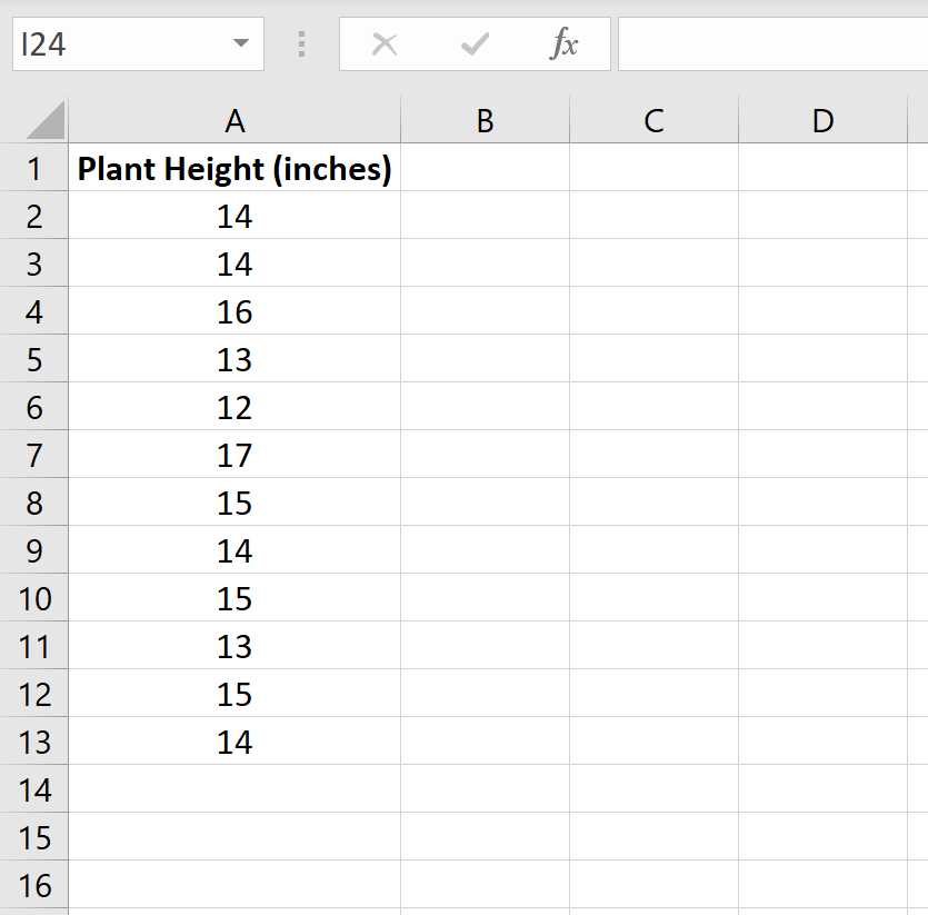
Suppose a botanist wants to know if the mean height of a certain species of plant is equal to 15 inches. She collects a random sample of 12 plants and records each of their heights in inches.
The following image shows the height (in inches) for each plant in the sample:

We can use the following steps to conduct a one sample t-test to determine if the mean height for this species of plant is actually equal to 15 inches.
Step 1: Find the sample size, sample mean, and sample standard deviation.
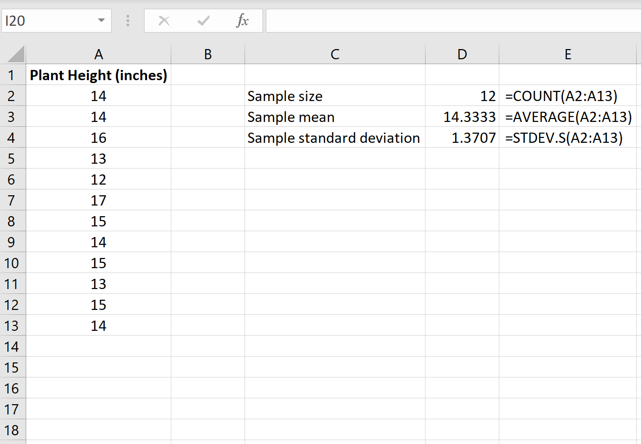
First, we need to find the sample size, sample mean, and sample standard deviation, which will all be used to conduct the one sample t-test.
The following image shows the formulas we can use to calculate these values:

Step 2: Calculate the test statistic t .
Next, we will calculate the test statistic t using the following formula:
t = x – µ / (s/√ n )
x = sample mean
µ = hypothesized population mean
s = sample standard deviation
n = sample size
The following image shows how to calculate t in Excel:

The test statistic t turns out to be -1.68485 .
Step 3: Calculate the p-value of the test statistic.
Next, we need to calculate the p-value associated with the test statistic using the following function in Excel:
=T.DIST.2T(ABS(x), deg_freedom)
x = test statistic t
deg_freedom = degrees of freedom for the test, which is calculated as n-1
Technical Notes: The function T.DIST.2T() returns the p-value for a two-tailed t-test. If you’re instead conducting a left-tailed t-test or a right-tailed t-test, you would instead use the functions T.DIST() or T.DIST.RT() , respectively.
The following image shows how to calculate the p-value for our test statistic:

The p-value turns out to be 0.120145 .
Step 4: Interpret the results.
The two hypotheses for this particular one sample t test are as follows:
H 0 : µ = 15 (the mean height for this species of plant is 15 inches)
H A : µ ≠15 (the mean height is not 15 inches)
Because the p-value of our test (0.120145) is greater than alpha = 0.05, we fail to reject the null hypothesis of the test.
We do not have sufficient evidence to say that the mean height for this particular species of plant is different from 15 inches.
Additional Resources
The following tutorials explain how to perform other common types of t-tests in Excel:
How to Conduct a Two Sample t-Test in Excel How to Conduct a Paired Samples t-Test in Excel
Featured Posts

Hey there. My name is Zach Bobbitt. I have a Masters of Science degree in Applied Statistics and I’ve worked on machine learning algorithms for professional businesses in both healthcare and retail. I’m passionate about statistics, machine learning, and data visualization and I created Statology to be a resource for both students and teachers alike. My goal with this site is to help you learn statistics through using simple terms, plenty of real-world examples, and helpful illustrations.
Leave a Reply Cancel reply
Your email address will not be published. Required fields are marked *
- DNA/RNA Analysis
- Lab Recipes
- GraphPad Prism
- Calculators

How To Perform A One-Sample T-Test In Excel
In this tutorial, I will show you how to perform a one-sample T-test by using Microsoft Excel.
What is a one-sample T-test?
A one-sample T-test is a statistical test to determine if a sample mean is significantly different from a hypothesized mean.
Example data
For this tutorial, I have a sample of 12 young female adults (18 years old). I measured their height in inches and entered the data into a single column in Excel.
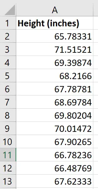
For the purpose of this example, I will pretend the national average height of 18-year-old girls is 66.5 inches.
I want to perform a one-sample T-test in Excel to determine if there is any significant difference between the heights of my sample compared with the national average height (66.5 inches).
The null and alternative hypothesis are:
- Null hypothesis – There is no significant difference between the heights of the sample, compared with the national average
- Alternative hypothesis – There is a significant difference between the heights of the sample, compared with the national average
How to perform a one-sample T-test in Excel
There is no function in Excel to perform a one-sample T-test. Instead, I will show you a step-by-step process on how to achieve this.
Firstly, calculate the mean, standard deviation (SD) and standard error of the mean (SEM) in Excel. Then, use this information to determine the t-statistic and ultimately the p-value.
Step 1: Calculate the average
The first thing you should do is to calculate the average value of the sample data.
This can be easily calculated by using the AVERAGE function in Excel.
In Excel, click on an empty cell and enter the following…
Replace cell1 in the equation with the cell containing the first data point and replace cell2 with the cell containing the last data point.
Below is a screenshot of what my example looks like.
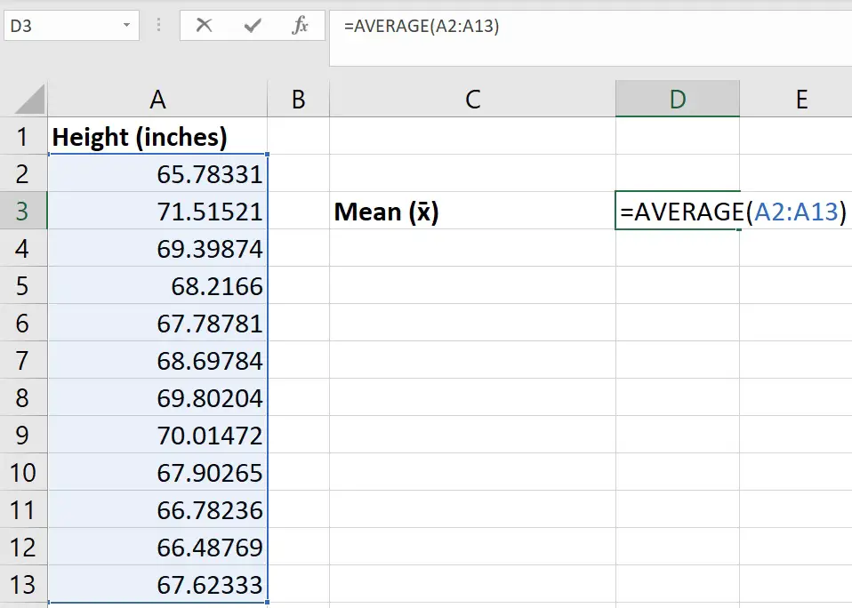
Step 2: Calculate the standard deviation
The next step is the calculate the SD of the sample data.
To do this, use the STDEV function.
In an empty cell, enter the following…
Again, replace cell1 and cell 2 in the equation with the cell containing the first and last data points, respectively.
Note, you can also use the STDEV.S function to achieve the same result.
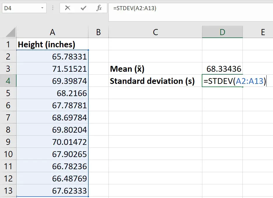
Step 3: Calculate the number of observations
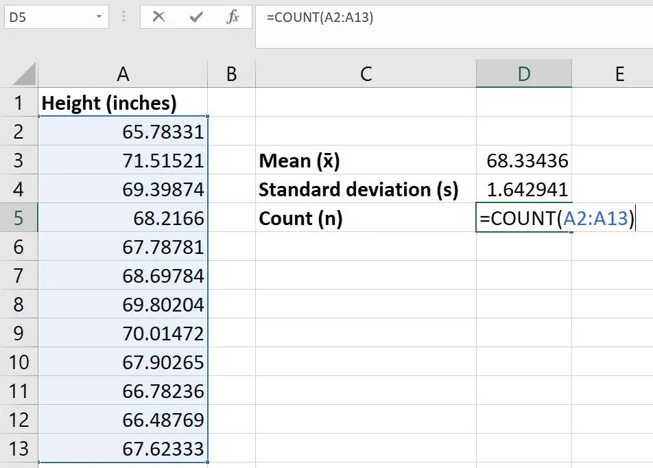
For the next step, simply count the number of observations in the sample.
This can be easily done if you have relatively small numbers. Otherwise, use the COUNT function to get Excel to count them for you.
As before, replace the cell1 and cell2 with the respected first and last cells.
Step 4: Calculate the standard error of the mean
Now we have the mean and n, we can now work out the standard error of the mean (SEM) .
To manually calculate the SEM, simply divide the SD by the square root of n.
Replace the following:
- SD – With the cell containing the SD
- n – With the cell containing the n
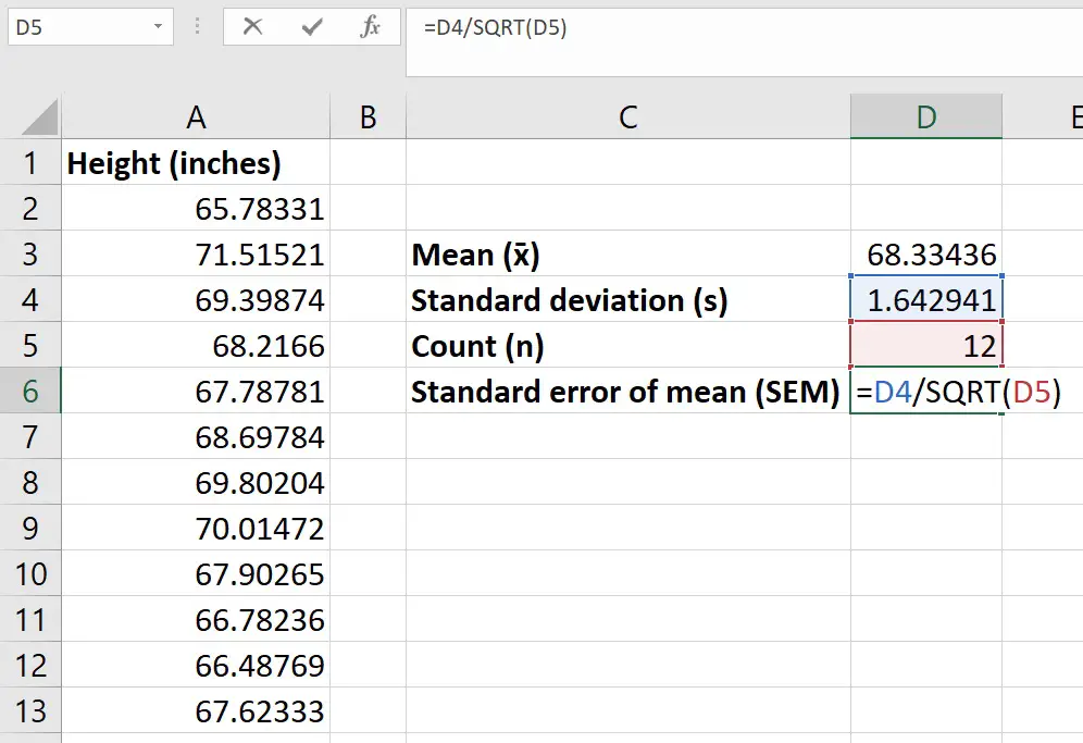
Step 5: Calculate the degrees of freedom
To calculate the degrees of freedom (df) in this case, simply subtract 1 from the n.
In a new cell, enter the following…
Replace n with the cell containing the n.
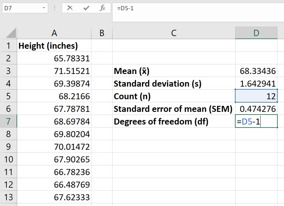
Step 6: Calculate the t-statistic
Before calculating the t-statistic, enter the hypothesized mean into a new cell in Excel.
The hypothesized mean is the value you want to compare your sample data to. So, in my example, this will be the national average height of 18-year-old girls – 66.5.
The formula to calculate the t-statistic for a one-sample T-test is shown below.

- x̄ – The sample mean
- μ – The hypothesized mean; in this case, the population mean
- s x̄ – The SEM
So, to work this out in Excel, click on an empty cell and enter the following…
Replace each component of the formula with the cell containing the corresponding value.
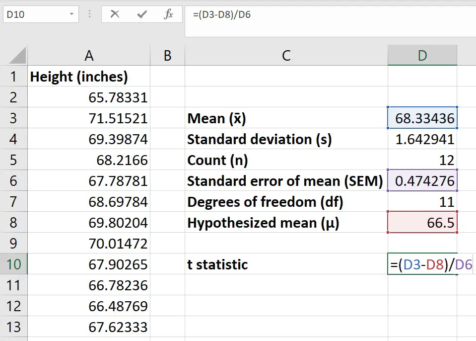
Step 7: Calculate the p-value
The last step is to calculate the p-value by using the t-statistic and the df. This is achieved by using the TDIST function.
Replace the following components of the function with…
- t – The cell containing the t-statistic
- df – The cell containing the df
- tails – Enter 1 if you want to perform a one-tailed analysis, or a 2 if you want to do a two-tailed analysis
For my example, I did not hypothesize if my sample data was greater or lower than the national average. Therefore, I will perform a two-tailed analysis.
If I hypothesized the sample data will be greater than the national average, then I would select to do a one-tailed analysis instead.
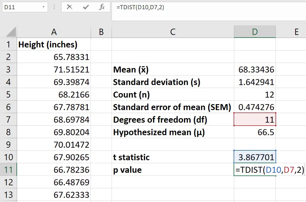
So, the p-value for my example is 0.0026.
If my alpha level was set at 0.05, then since the p-value is below the alpha level, I will reject the null hypothesis and accept the alternative hypothesis.
In other words, there is a significant difference between the heights of the sample, compared with the national average.
Wrapping up
In this tutorial, I have shown you how to perform a one-sample T-test in Excel. There is no function to perform a one-sample T-test in Excel. However, you can still perform this by using a stepwise approach.
Microsoft Excel version used: 365 ProPlus
RELATED ARTICLES MORE FROM AUTHOR
How To Perform Descriptive Statistics In Microsoft Excel

How To Do Basic Math In Excel (Add, Subtract, Multiply & Divide)

How To Calculate A Weighted Average In Microsoft Excel
OMG!. Thank you sooooo much! I’ve been in statistics hell and this is exactly what I was looking for. The process is explained well and had all of the formulas I needed to do both the test statistic and p value.
LEAVE A REPLY Cancel reply
Save my name, email, and website in this browser for the next time I comment.
Other Excel tutorials
How to perform random sampling in microsoft excel, how to perform a chi-square test of independence in excel, stay connected.

Dr. Matt C. Howard
My research interests include (1) statistics and methodologies, (2) health and well-being, (3) personality and individual differences, as well as (4) technology-enhanced training and development., one-sample t-test in excel.
I don’t come across the need to perform a one-sample t-test that often, whether in research or practice. However, it is a very good entry into learning about two-sample t-tests and ANOVAs, so I teach it early in my undergraduate statistics courses. I get slightly annoyed whenever I teach it, though, because Excel does not have the one-sample t-test built into its Data Analysis add-on. Nevertheless, we can trick Excel into performing it for us, which I detail below. If you have any questions, please email me at [email protected] .
The purpose of a one-sample t-test is pretty simple. It tells us whether the mean of a variable is significantly different than a chosen value, and it can be used to answer the following questions:
- Is a basketball team’s average height significantly different than 6’6″?
- Is a company’s yearly revenue significantly different than 10 million dollars?
- Is the job satisfaction of a company’s employees significantly different than a 4 on a 1 to 7 scale?
These questions may be interesting, but they don’t occur all that often in research or practice, and selecting an arbitrary value to test isn’t typically informative. Nevertheless, some examples in which a one-sample t-test may be useful are:
- When you know a pre-defined value is important.
- When you have a certain expected value for a sample.
- When there is some common-sense value.
- When you are performing a replication study.
Of course, there are other situations in which a one-sample t-test may be useful, so keep your eyes open for these situations!
Now that we know what a one-sample t-test is used for, we can now calculate a one-sample t-test in Excel. To begin, open your data in Excel. If you don’t have a dataset, download the example dataset here. In the example dataset, we are comparing the test grades of a class to the chosen value of 80. This will determine whether the students’ average grades are significantly different from a value of 80.
The data should look like the image below.

Now, we need to start by tricking Excel into calculating the one-sample t-test for us. Let’s start by typing three things into the second column. In the first row, type the word “Number” (without quotation marks), which is our label. In the second and third row, type the number that you want to compare the data against. In the current example, we chose the number “80”. So, type “80” (without quotation marks) into the second and third rows of the second column. Your Excel should look like the image below:

With the numbers entered, now click on the Data tab at the top, and then click on the Data Analysis button. If you do not have this in your version of Excel, check out my page on Activating Data Analysis in Excel .

The following window should pop up. This is where it gets a little confusing. Although we are performing a one-sample t-test, you should click on “t-Test: Two-Sample Assuming Unequal Variances” and then click on “OK”. Because Excel does not have a one-sample t-test command, we must trick it into thinking those two numbers that we typed are another sample. Confusing, I know, but it works!

Now, click on the button highlighted below:

And then click and drag overtop all the data in Column A. In this example, I do NOT include the label. Just click and drag on the numbers in the first column, and then press the highlighted button.

Click on the other button highlighted below:

And do the same thing, but highlight the numbers in the second column. If you are using the example dataset, you should highlight the two number 80s. Then press the highlighted button.

You should get results. Yay! Take a look at the image below and compare your results. Did you get the same numbers? If so, great! If not, start from the beginning and try it again.

So what do these numbers tell us? First, look at the highlighted number below. In the current example, we have an average of 90.9. This means the class’s test grade was, on average, a 90.9. Already, we can tell that this is larger than our chosen number of 80.

Now, look at the number highlighted in the picture below. This is our t-statistic. It is our primary result or effect size, and it is 7.630 in the current example. Is that big? Is it small? It is fairly difficult to interpret, so it would be best to turn to our p-value.

The number highlighted below is our p-value. It is listed as 2.01E-08. How does a number have an “E” in it? Well, when a number is extremely small or large in Excel, it is sometimes reported in scientific notation. The number after the E represents how many spaces we should move the decimal point. If it is positive, we move the decimal to the right and make the number bigger. If it is negative, we move the decimal to the left and make the number smaller.

So, the current result of 2.01E-08 is actually .0000000201. That is very, very small for a p-value – much less than our cutoff of .05. Because our p-value is less than .05, then we would consider our results statistically significant. If a one-sample t-test result is statistically significant, we would say that our mean is significantly different than the chosen value. In the current example, we would say that the class average is significantly different than a value of 80. Then, we could look at the mean (90.9) to determine that our class mean is significantly larger than a value of 80, because the mean is both significantly different and larger than a value of 80.
That is all for the one-sample t-test in Excel! If you have any questions, please contact me at [email protected] .
Share this:

- Already have a WordPress.com account? Log in now.
- Subscribe Subscribed
- Copy shortlink
- Report this content
- View post in Reader
- Manage subscriptions
- Collapse this bar
How to Do a T Test in Excel (2 Ways with Interpretation of Results)
The article will show you how to do a T Test in Excel. T-Tests are hypothesis tests that evaluate one or two groups’ means. Hypothesis tests employ sample data to infer population traits. In this lesson, we will look at the different types of T-Tests , and how to run T-Tests in Excel. We’ll go over both paired and two sample T-Tests , with detailed instructions on how to prepare your data, run the test, and interpret the findings.
Understanding how to use the T.TEST function in Excel will improve your ability to draw significant insights and make data-driven decisions, whether you’re a student, researcher, business analyst, or anybody else who works with data. Let’s say, you’re doing education research to assess the efficacy between traditional and new approaches. T-tests will guide you through providing the mean scores of students based on the approaches that they were taught. So that, you can make a decision based on the students’ performance.
Download Practice Workbook
T Test.xlsx
T Test Type
There are basically two types of t-tests. They are:
- One-tailed t-test
- Two-tailed t-test
Each of them has 3 types. They are:
- Two sample equal variance
- Two sample unequal variance
We will show you the application of some of these types. The procedure of getting the results for all types of t-tests in Excel are the same. Let’s dig into some details and see how it can be done.
How to Do a T Test in Excel: 2 Effective Ways
1. using excel t.test or ttest function to do t test.
Here, we are going to show you how to determine the T Test result by using formulas. Excel has T.TEST and TTEST functions to operate t-test on different variables. Both functions work similarly. First, we will cover how to determine the t-test value of two sample variables with equal variance.
1.1 Two Sample Equal Variance T Test
In the dataset, you will see the prices of different laptops and smartphones. Here is a formula that performs a T Test on the prices of these products and returns the t-test result.
=T.TEST(B5:B14,C5:C14,2,2)
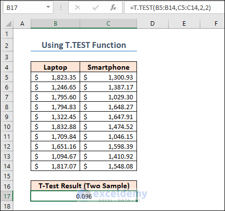
We set the 3rd argument of the function to 2 as we are doing a two tailed t-test on the dataset. The 4th argument should be 2 for a two sample equal variance t-test.
1.2 Paired T Test
Now, we are going to apply another formula to calculate the Paired T-Test . The following dataset shows the performance mark of some employees in two different criteria.
=T.TEST(C5:C13,D5:D13,2,1)
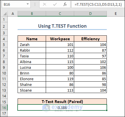
Note: The explanation of the results is described in the following sections.
2. Using Analysis Toolpak
The above tasks can be done with the Analysis Toolpak Add-in too. The Analysis Toolpak Add-in is not available in the ribbon by default. To initiate it,
- Go to the Options window first.
- Next, select Add-ins and click on the Go button beside the Manage section.
- After that, click OK .

- Thereafter, the Add-ins window will appear. Select Analysis Toolpak >> click OK again.
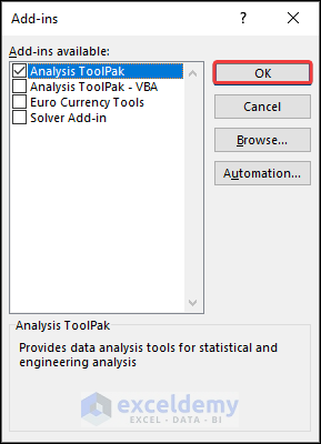
This Add-in will be added to the ribbon of the Data tab.
2.1 Two Sample Equal Variance T Test
We will do a two sample equal variance t-test using the Analysis Toolpak here. We used the dataset that contains the prices of laptops and smartphones. For this purpose,
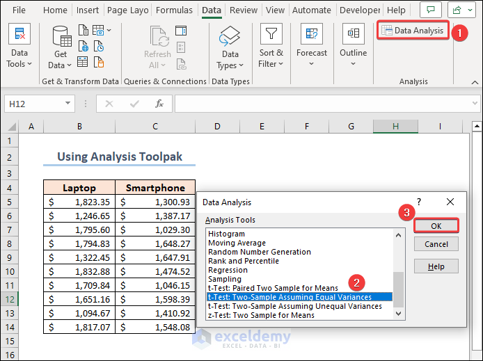
- Click on the Data Analysis button from the ribbon of the Data tab.
- The Data Analysis features will appear. Select t-Test: Two Sample Assuming Equal Variances and click OK .
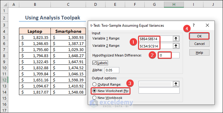
- After that, you need to set up the parameters for the t-test operation. Insert the Laptop and Smartphone prices as Variable 1 Range and Variable 2 Range Include the headings in the range and check Labels.
- Next, set the value of Hypothesized Mean Difference to 0 .
- Finally, select an Output option of your preference and click OK .
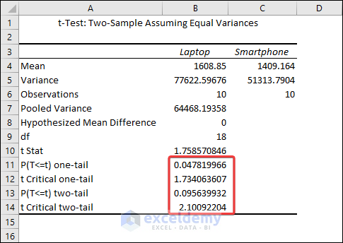
As we have chosen a New Worksheet for the outputs, we will see the results in a new sheet.
Now, let’s get to the discussion on the results.
Comments on Results
The output shows that the mean values for Laptops and Smartphones are 1608.85 and 1409.164 respectively. We can see from the Variances row that they are not precisely equal, but they are close enough to be assumed to have equal variances. The most relevant metric is the p-value .
The difference between means is statistically significant if the p-value is less than your significance level. Excel calculates p-values for one- and two-tailed T Tests .
One-tailed T Tests can detect only one direction of difference between means. A one-tailed test, for example, might only evaluate whether Smartphones have higher prices than Laptops . Two-tailed tests can reveal differences that are larger or smaller than. There are some other disadvantages to utilizing one-tailed testing, so I’ll continue with the conventional two-tailed results.
For our results, we’ll utilize P(T=t) two-tail, which is the p-value for the t-test’s two-tailed version. We cannot reject the null hypothesis because our p-value ( 0.095639932 ) is greater than the conventional significance level of 0.05 . The hypothesis that the population means differ is supported by our sample data. The mean price of Laptops is greater than the mean price of Smartphones’ .
The Analysis Toolpak operation also returns results for one-tailed t-test . Here, the one-tailed P value of two sample equal variance t-test is 1.734 .
2.2 Paired T Test
Similarly, you can find out the Paired t-Test result for the dataset containing employee performances. Just select the t-Test: Paired Two Samples for Mean when you open the Data Analysis window.
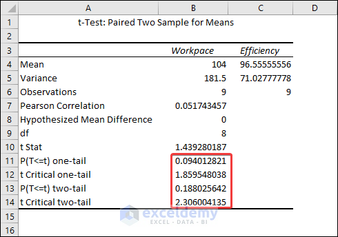
The result shows that the mean for the Workpace is 104 and the mean for the Efficiency is 96.56 .
The difference between means is statistically significant if the p-value is less than your significance level. For our results, we’ll utilize P(T=t) two-tail, which is the p-value for the t-test’s two-tailed version. We cannot reject the null hypothesis because our p-value ( 0.188 ) is greater than the conventional significance level of 0.05 . The hypothesis that the population means differ is supported by our sample data. In particular, the Workpace mean exceeds the Efficiency mean.
How to Interpret t-Test Results in Excel
Although we explained the results of the t-Test earlier, we didn’t show the proper interpretation. So here, I’ll show you the interpretation of the two sample equal variance t-test.
Let’s bring out the results again first.
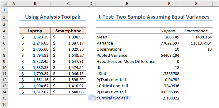
- The mean of laptop prices = 1608.85
- The mean of smartphone prices = 1409.164
ii. Variance
- The variance of laptop prices = 77622.597
- The variance of smartphone prices = 51313.7904
iii. Observations
The number of observations for both laptops and smartphones are 10 .
iv. Pooled Variance
The samples’ average variance, calculated by pooling the variances of each sample.
The mathematical formula for this parameter is:
((No of observations of Sample 1-1)*(Variance of Sample 1) + (No of observations of Sample 2-1)*(Variance of Sample 2))/(No of observations of Sample 1 + No of observations of Sample 2 – 2)
So it becomes: ((10-1)*77622.59676+(10-1)*51313.7904)/(10+10-2) = 64468.19358
v. Hypothesized Mean Difference
We “hypothesize” that the number is the difference between the two population means. In this situation, we chose 0 because we want to see if the difference between the means of the two populations is zero.
It indicates the value of the Degrees of Freedom. Formula for this parameter is:
No of observations of Sample 1 + No of observations of Sample 2 – 2 = 10 + 10 – 2 = 18
vii. t Stat
The test statistic value of the t-Test operation.
The formula for this parameter is given below.
(Mean of Sample 1 – Mean of Sample 2)/(Square root of (Pooling Variance* (1/No of observations of Sample 1 + 1/No of observations of Sample 2)))
So it becomes: (1608.85 – 1409.164)/Sqrt(64468.19358 * (1/10 + 1/10)) = 1.758570846
viii. P(T<=t) two-tail
A two-tailed t-test’s p-value. This value can be found by entering t = 1.758570846 with 18 degrees of freedom into any T Score to P Value Calculator.
In this situation, the value of p is 0.095639932 . Because this is greater than 0.05 , we cannot reject the null hypothesis. This suggests that we lack adequate evidence to conclude that the two population means differ.
ix. t Critical two-tail
This is the test’s crucial value. A t Critical value Calculator with 18 degrees of freedom and a 95% confidence level can be used to calculate this number.
In this instance, the critical value is 2.10092204 . We cannot reject the null hypothesis because our test statistic t is less than this number. Again, we lack adequate information to conclude that the two population means are distinct.
Things to Remember
- Excel demands that your data be arranged in columns, with data from each group in a separate column. The first row should have labels or headers.
- Clearly state your null hypothesis (usually that there is no significant difference between the group means) and your alternative hypothesis (the opposite of the null hypothesis).
- As a result of the t-test, Excel returns the p-value. A little p-value (usually less than the specified alpha level) indicates that the null hypothesis may be rejected and that there is a substantial difference between the group means.
Frequently Asked Questions
1. Can I perform a t-test on unequal sample sizes in Excel?
Answer: Yes, you can use the T.TEST function to do a t-test on unequal sample sizes. When calculating the test statistic, Excel automatically accounts for unequal sample sizes.
2. What is the difference between a one-tailed and a two-tailed t-test?
Answer: A one-tailed t-test determines if the means of the two groups differ substantially in a given direction (e.g., greater or smaller). A two-tailed t-test looks for any significant difference, regardless of direction.
3. Can I calculate effect size in Excel for t-tests?
Answer: While there is no built-in tool in Excel to calculate effect size, you may manually compute Cohen’s d for independent t-tests and paired sample correlations for paired t-tests using Excel’s basic mathematical operations.
In the end, we can conclude that you will learn some basic ideas on how to do a t Test in Excel. If you have any questions or feedback regarding this article, please share them in the comment section. Your valuable ideas will enrich my Excel expertise and hence the content of my upcoming articles.
<< Go Back to Statistical Significance in Excel | Excel for Statistics | Learn Excel

What is ExcelDemy?
Tags: Statistical Significance in Excel

Md. Meraz Al Nahian has worked with the ExcelDemy project for over 1.5 years. He wrote 140+ articles for ExcelDemy. He also solved a lot of user problems and worked on dashboards. He is interested in data analysis, advanced Excel, statistics, and dashboards. He also likes to explore various Excel and VBA applications. He completed his graduation in Electrical & Electronic Engineering from Bangladesh University of Engineering & Technology (BUET). He enjoys exploring Excel-related features to gain efficiency... Read Full Bio
Leave a reply Cancel reply
ExcelDemy is a place where you can learn Excel, and get solutions to your Excel & Excel VBA-related problems, Data Analysis with Excel, etc. We provide tips, how to guide, provide online training, and also provide Excel solutions to your business problems.
Contact | Privacy Policy | TOS
- User Reviews
- List of Services
- Service Pricing

- Create Basic Excel Pivot Tables
- Excel Formulas and Functions
- Excel Charts and SmartArt Graphics
- Advanced Excel Training
- Data Analysis Excel for Beginners

Advanced Excel Exercises with Solutions PDF

How to Conduct a One Sample t-Test in Excel
A one sample t-test is used to test whether or not the mean of a population is equal to some value.
This tutorial explains how to conduct a one sample t-test in Excel.
Suppose a botanist wants to know if the mean height of a certain species of plant is equal to 15 inches. She collects a random sample of 12 plants and records each of their heights in inches.
The following image shows the height (in inches) for each plant in the sample:
We can use the following steps to conduct a one sample t-test to determine if the mean height for this species of plant is actually equal to 15 inches.
Step 1: Find the sample size, sample mean, and sample standard deviation.
First, we need to find the sample size, sample mean, and sample standard deviation, which will all be used to conduct the one sample t-test.
The following image shows the formulas we can use to calculate these values:
Step 2: Calculate the test statistic t .
Next, we will calculate the test statistic t using the following formula:
t = x – µ / (s/√ n )
x = sample mean
µ = hypothesized population mean
s = sample standard deviation
n = sample size
The following image shows how to calculate t in Excel:
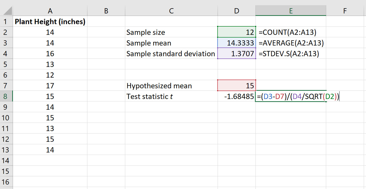
The test statistic t turns out to be -1.68485 .
Step 3: Calculate the p-value of the test statistic.
Next, we need to calculate the p-value associated with the test statistic using the following function in Excel:
=T.DIST.2T(ABS(x), deg_freedom)
x = test statistic t
deg_freedom = degrees of freedom for the test, which is calculated as n-1
Technical Notes: The function T.DIST.2T() returns the p-value for a two-tailed t-test. If you’re instead conducting a left-tailed t-test or a right-tailed t-test, you would instead use the functions T.DIST() or T.DIST.RT() , respectively.
The following image shows how to calculate the p-value for our test statistic:
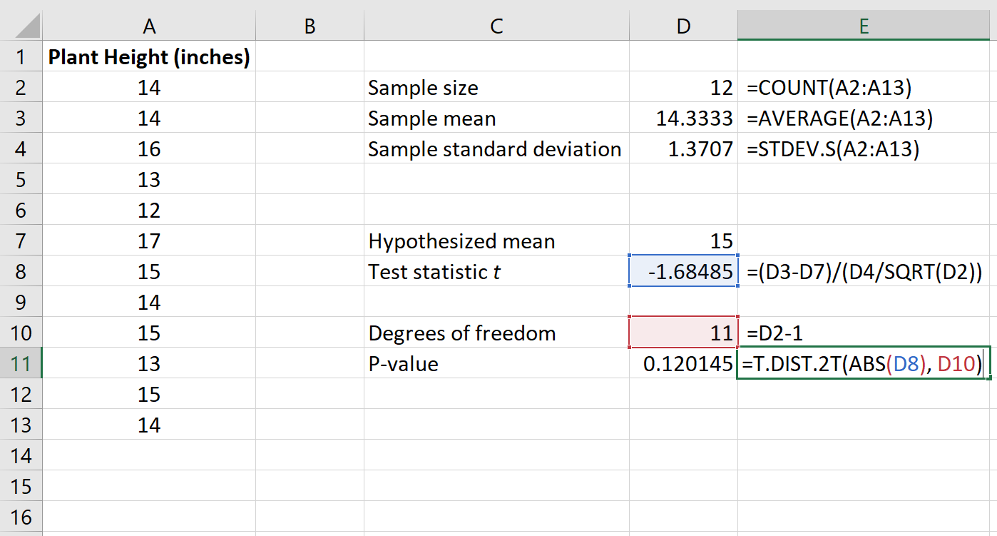
The p-value turns out to be 0.120145 .
Step 4: Interpret the results.
The two hypotheses for this particular one sample t test are as follows:
H 0 : µ = 15 (the mean height for this species of plant is 15 inches)
H A : µ ≠15 (the mean height is not 15 inches)
Because the p-value of our test (0.120145) is greater than alpha = 0.05, we fail to reject the null hypothesis of the test.
We do not have sufficient evidence to say that the mean height for this particular species of plant is different from 15 inches.
Additional Resources
The following tutorials explain how to perform other common types of t-tests in Excel:
How to Conduct a Two Sample t-Test in Excel How to Conduct a Paired Samples t-Test in Excel
A Simple Explanation of Internal Consistency
How to perform simple linear regression in stata, related posts, how to create a stem-and-leaf plot in spss, how to create a correlation matrix in spss, excel: how to use if function with text..., excel: how to use greater than or equal..., excel: how to use if function with multiple..., how to convert date of birth to age..., excel: how to highlight entire row based on..., how to add target line to graph in..., excel: how to use if function with negative..., how to extract number from string in pandas.

Excel Tutorial: How To Do A Hypothesis Test In Excel
Introduction.
Welcome to our Excel tutorial on how to conduct a hypothesis test using Excel. Hypothesis testing is a crucial component of statistical analysis, allowing us to make inferences about a population based on sample data. Using Excel for hypothesis testing offers several advantages, including its familiarity, ease of use, and the ability to perform complex statistical calculations with just a few clicks.
Key Takeaways
- Hypothesis testing is essential for making inferences about a population based on sample data.
- Using Excel for hypothesis testing offers familiarity, ease of use, and the ability to perform complex statistical calculations.
- Organizing and formatting data correctly in Excel is crucial for hypothesis testing.
- Understanding the different types of hypothesis tests and selecting the appropriate test is important for accurate analysis.
- Interpreting the results of the hypothesis test and avoiding common mistakes is essential for making valid conclusions.
Setting up the data in Excel
When conducting a hypothesis test in Excel, it is crucial to properly organize and format your data in a spreadsheet. This will ensure accurate and reliable results.
- Start by opening a new Excel spreadsheet and entering your raw data into the cells. It is important to have a clear understanding of the variables you are working with and how they relate to each other.
- Label each column with a clear and descriptive header to identify the variables being tested. This will help you keep track of the data and make it easier to analyze.
- Arrange the data in a logical and organized manner, such as grouping similar data together and using separate columns for different variables.
- Check that the data is formatted correctly, especially if it includes dates, currency, or percentages. Use the appropriate formatting options in Excel to ensure the data is displayed accurately.
- Remove any unnecessary formatting, such as extra spaces or special characters, to avoid errors in the analysis process.
- Double-check for any missing or erroneous data entries, and make sure that the data is complete and accurate before proceeding with the hypothesis test.
Choosing the Appropriate Test in Excel
When conducting a hypothesis test in Excel, it's crucial to choose the right test for your specific scenario. Understanding the different types of hypothesis tests and how to select the appropriate one is essential for accurate and meaningful results.
Parametric Tests:
Nonparametric tests:, one-sample, two-sample, and paired tests:, goodness-of-fit tests:, chi-square tests:.
Choosing the right hypothesis test in Excel requires careful consideration of the nature of the data and the specific research question. Here are some key factors to consider when selecting the appropriate test:
- Understanding the Data: Determine whether the data is continuous or categorical, and whether it follows a specific distribution.
- Research Question: Clearly define the research question and the type of comparison or relationship being investigated.
- Sample Size: Consider the size of the sample and whether it meets the assumptions of the chosen test.
- Dependent or Independent Variables: Determine whether the variables are independent or related in some way, as this will impact the choice of test.
- Assumptions: Ensure that the chosen test aligns with any specific assumptions or conditions required for accurate results.
Conducting the hypothesis test
When it comes to conducting a hypothesis test in Excel, there are a few key steps to follow in order to ensure accurate results. These steps include using the Data Analysis Toolpak and inputting the necessary parameters for the test.
The Data Analysis Toolpak is a powerful add-in for Excel that provides a variety of data analysis tools, including the ability to conduct hypothesis tests. To access the Toolpak, simply go to the "Data" tab, click on "Data Analysis" in the Analysis group, and select "t-Test: Two-Sample Assuming Equal Variances" for a two-sample t-test, or "t-Test: Paired Two Sample for Means" for a paired t-test.
Once the Data Analysis Toolpak is open, you will need to input the necessary parameters for the hypothesis test. This includes selecting the appropriate variables for analysis, specifying the significance level, and choosing whether to perform a one-tailed or two-tailed test. It is important to carefully review and input the correct parameters to ensure the accuracy of the test results.
By using the Data Analysis Toolpak in Excel and inputting the necessary parameters for the hypothesis test, you can effectively conduct hypothesis tests and analyze your data with confidence.
Interpreting the results
After performing a hypothesis test in Excel, it is important to understand how to interpret the results and make conclusions based on the data.
Identify the test statistic:
Look at the p-value:, consider the confidence interval:, check for statistical significance:, reject or fail to reject the null hypothesis:, consider the practical significance:, communicate the findings:, common mistakes to avoid.
When conducting a hypothesis test in Excel, there are some common mistakes that researchers often make. By being aware of these pitfalls, you can ensure that your results are accurate and reliable.
One of the most common mistakes when doing a hypothesis test in Excel is misinterpreting the results. It's important to carefully analyze the output of the test and understand what it is telling you. Avoid jumping to conclusions without thoroughly examining the data and the significance level.
Another mistake to avoid is using the wrong test for the hypothesis you are trying to test. Excel offers a variety of hypothesis tests, such as t-tests, F-tests, and chi-squared tests, among others. It's crucial to select the appropriate test for your specific research question and data set. Using the wrong test can lead to inaccurate results and conclusions.
In conclusion, hypothesis testing in Excel is a crucial tool for making data-driven decisions in various fields, from business to science. By using Excel, we can effectively analyze data and draw meaningful conclusions about our hypotheses.
As with any skill, practice makes perfect . So, I encourage you to continue exploring and practicing hypothesis testing in Excel. There are numerous resources available online that provide additional guidance and examples to help you master this valuable technique.

Immediate Download
MAC & PC Compatible
Free Email Support
Related aticles

The Benefits of Excel Dashboards for Data Analysts

Unlock the Power of Real-Time Data Visualization with Excel Dashboards

Unlocking the Potential of Excel's Data Dashboard

Unleashing the Benefits of a Dashboard with Maximum Impact in Excel

Exploring Data Easily and Securely: Essential Features for Excel Dashboards

Unlock the Benefits of Real-Time Dashboard Updates in Excel

Unleashing the Power of Excel Dashboards

Understanding the Benefits and Challenges of Excel Dashboard Design and Development

Leverage Your Data with Excel Dashboards

Crafting the Perfect Dashboard for Excel

An Introduction to Excel Dashboards

How to Create an Effective Excel Dashboard
- Choosing a selection results in a full page refresh.
One sample t-test or z-test in Excel tutorial
This tutorial shows how to test the difference between an observed mean and a theoretical one, using the one sample t-test and z-tests , in Excel with XLSTAT.
Dataset to perform a mean comparison test - either a Student's t-test or a z-test
The data correspond to the mathematic grade average for the first semester of a class of 33 students.
Goal 1 of this tutorial
We want to compare the results of those students with the county average which is 11.5. We don’t have the information about the variance of this statistic so we cannot run a z-test. We will then run a t-test.
The class average is 11.121. Descriptive statistics on the class performance can be computed using the function Descriptive Statistics .
We can use a t-test to determine if the difference between the average of the class and the average of all students in the county are similar or different with a risk of 5%.
Setting up a Student's t-test for comparing the mean of a sample to a value

In the dialog box, select the data. Press the Range selector and select the column B that contains the “Math average”. The data format is One sample per column . Here we have only one column corresponding to one sample to test. If the data were spanned on several columns for the same sample we could use the other option.
The results will be displayed in a new sheet as we keep the default option Sheet .
The name of the column was included in our data selection so we tick the option Column labels .
Finally, you have to decide if you want to run a t-test or a z-test. As explained above we don’t have the information about the standard deviation of the population so we have to run a Student’s t test .

We can move on to the tab Options to specify our analysis. The first thing to select is the alternative hypothesis. We know that the average of the class is inferior to the general average so we can select the option Mean 1 < Theoretical mean to run a one-sided test which is more accurate than a two-sided test.
Then we enter 11.5 in the Theoretical mean field. The default significance level is 5%. We will use this value.

In the Missing data tab, we can choose any option as we do not have missing data in this dataset. For the last section Outputs , we select the only available option Descriptive statistics .

When everything is set, press OK .
Results of the Student's t-test to compare the mean of a sample to a value
The results of the t-test appear in a new sheet. The following table shows that we cannot reject the null hypothesis Ho so we may suggest that the average class performance is as good as the average performance of the country.

Goal 2 of this tutorial
To go further we can now use the standard deviation for the math grades for the county. Let’s use 0.55. So the variance is 0.3025.
Setting up a z-test for the comparison of the mean of a sample to a value
In the first tab General , this time instead of the Student’s t-test option choose the option z-test .

In the Options tab, you need to set the variance for the z-test. Opt for the option User defined and set the value to 0.3025.

Results and interpretation of a z-test for the comparison of the mean of a sample to a value
In the results page you now have that the hypothesis H0 should be rejected and that the students performed significantly worse than the students of the county.

The following video shows how to run a Student's t-test and a z-test in XLSTAT.
Was this article useful?
Similar articles
- Compare two proportions in Excel tutorial
- Student's t test on two independent samples tutorial
- Compare ≥ 2 samples described by several variables
- Compare k proportions in Excel tutorial
- One proportion test in Excel tutorial
- One sample variance test in Excel tutorial
Expert Software for Better Insights, Research, and Outcomes

IMAGES
VIDEO
COMMENTS
The following image shows how to calculate t in Excel: The test statistic t turns out to be -1.68485. Step 3: Calculate the p-value of the test statistic. Next, we need to calculate the p-value associated with the test statistic using the following function in Excel: =T.DIST.2T (ABS (x), deg_freedom) where: x = test statistic t.
T1_TEST (R1, hyp, tails) = the p-value of the one-sample t-test for the data in array R1 based on the hypothetical mean hyp (default 0) where tails = 1 or 2 (default). For Example 2, the formula T1_TEST (A5:D14, 78, 2) will output the same value shown in cell Q56 of Figure 5, namely p-value = .000737.
Step 2: Calculate the standard deviation. The next step is the calculate the SD of the sample data. To do this, use the STDEV function. In an empty cell, enter the following…. =STDEV(cell1:cell2) Again, replace cell1 and cell 2 in the equation with the cell containing the first and last data points, respectively.
Paired t-tests and 1-sample t-tests are the same hypothesis test incognito!" So, a question - can one, using excel's paired t-test function, put sample data in the first column and the null hypothesis value, repeatedly, in the second column and "trick" excel into running a one sample t-test using the paired t-test function?
The data should look like the image below. Now, we need to start by tricking Excel into calculating the one-sample t-test for us. Let's start by typing three things into the second column. In the first row, type the word "Number" (without quotation marks), which is our label. In the second and third row, type the number that you want to ...
Here is a formula that performs a T Test on the prices of these products and returns the t-test result. =T.TEST(B5:B14,C5:C14,2,2) We set the 3rd argument of the function to 2 as we are doing a two tailed t-test on the dataset. The 4th argument should be 2 for a two sample equal variance t-test.
This video shows how to conduct a one-sample hypothesis t-test for the mean in Microsoft Excel using the built-in Data Analysis (from raw data).How to load ...
She would write the hypotheses for this particular one sample t-test as follows: H 0: µ = 15; H A: µ ≠15; Refer to this tutorial for a step-by-step explanation of how to perform this hypothesis test in Excel. Example 2: Two Sample t-test in Excel. A two sample t-test is used to test whether or not the means of two populations are equal.
t = x - µ / (s/√n) where: x = sample mean. µ = hypothesized population mean. s = sample standard deviation. n = sample size. The following image shows how to calculate t in Excel: The test statistic t turns out to be -1.68485. Step 3: Calculate the p-value of the test statistic.
To access the Toolpak, simply go to the "Data" tab, click on "Data Analysis" in the Analysis group, and select "t-Test: Two-Sample Assuming Equal Variances" for a two-sample t-test, or "t-Test: Paired Two Sample for Means" for a paired t-test. B. Inputting the necessary parameters for the test. Once the Data Analysis Toolpak is open, you will ...
How to conduct One Sample t-test in Excel | Step by Step GuideThe one-sample t-test is a statistical hypothesis test used to determine whether an unknown pop...
One Sample T Test Hypotheses. A one sample t test has the following hypotheses: Null hypothesis (H 0): The population mean equals the hypothesized value (µ = H 0).; Alternative hypothesis (H A): The population mean does not equal the hypothesized value (µ ≠ H 0).; If the p-value is less than your significance level (e.g., 0.05), you can reject the null hypothesis.
This video provides the fundamental knowledge on One Sample Hypothesis Test and how to use Microsoft Excel to calculate the test statistics, critical value ...
Setting up a Student's t-test for comparing the mean of a sample to a value. Go over to the menu Parametric tests and select the option One-sample t-test and z-test . In the dialog box, select the data. Press the Range selector and select the column B that contains the "Math average". The data format is One sample per column.
In this article we will learn about One Sample z Test, forming the null and alternate hypothesis, p-value approach, critical value approach and how to use MS Excel to create it as your own ...
In this video, we will learn how to perform One sample t-test in Excel. We will learn to perform it by using excel functions and also by Data Analysis tool.I...
Hypothesis Test in Excel: Manual Steps. Step 1: Type your data into a single column in Excel. For example, type your data into cells A1:A40. Step 2: Click the "Data" tab and then click "Data Analysis.". If you don't see the Data Analysis button then you may need to load the Data Analysis Toolpak. Step 3: Click " Descriptive ...
In Excel, click Data Analysis on the Data tab. From the Data Analysis popup, choose F-Test Two-Sample for Variances. Under Input, select the ranges for both Variable 1 Range and Variable 2 Range. Check the Labels checkbox if you have meaningful variable names in row 1. This option makes the output easier to interpret.
Hypothesis T Test using Excel | One Sample Test | Two Sample Test | Data Analysis using Excel𝐓𝐢𝐦𝐞𝐋𝐢𝐧𝐞: 00:00 Introduction 01:46 Hypothesis Testing...