hypothesis test on ti 84 plus

Hypothesis Testing using the Z-Test on the TI-83 Plus, TI-84 Plus, TI-89, and Voyage 200

The TI-83 Plus and TI-84 Plus are optimized for performing many tasks in statistics, and one of their most powerful features is the ability to perform a variety of tests of statistical significance. With the statistics package installed, the TI-89, TI-92 Plus, and Voyage 200 also have much of this capability. This tutorial demonstrates how to use your graphing calculator to solve basic hypothesis testing problems such as the following using the Z-Test:

A researcher designs an experiment where a random sample of n = 50 high school seniors are given a pill to improve their concentration and problem solving skills. After being administered the pill, subjects take the SAT, and their scores on the SAT Math section are tabulated. The average score of student who took the pill is x̄ = 540. Given that the average score of all high school seniors on the SAT is μ = 510 with standard deviation σ = 100, is there statistically significant evidence that students who took the pill scored higher?

Before beginning the calculations, it is necessary to come up with specific hypotheses for the tests and choose a level of significance. In inferential statistics, there are two hypothesis, the null hypothesis, and the alternative hypothesis. The null hypothesis, denoted H₀, is always that the statistic measures of the treated group (in this case students given a pill) is the same as that for the general population. Since we are only interested in whether or not the pill has a positive effect, we are doing a one-tailed Z-Test, and our null hypothesis is:

H₀: μ <= μ₀

Where μ is the true mean (as opposed to sample mean) of scores of students in the treatment group. μ₀ refers to the known population mean, in this case 510. The alternative hypothesis H 1 is what we expect if the treatment does have an effect on the population, and is always the opposite of the alternative hypothesis. Our alternative hypothesis is:

H₁: μ > μ₀

Finally, we have to choose a level of significance (α) for our test. It is possible that even if the treatment has no effect, we could get a mean score of 540. This seems unlikely and the chances of this happening goes down with the more subjects in the study, but the purpose of hypothesis testing is first of all to avoid coming to the wrong conclusion. The level of significance is a threshold probability below which we say that we have found statistical evidence. It is considered good practice to choose this beforehand so that the statistician doesn’t change α after wards in order to “find” statistical evidence where there is none. For most problems, a level of significance is:

α = .05

This means that if we find there is less than a 5% chance that the sample mean is higher than 540 by chance alone, we will conclude statistical significance.

Performing a Z-Test on the TI-83 Plus and TI-84 Plus

From the home screen, press STAT ▶ ▶ to select the TESTS menu. “Z-Test” should already be selected, so press ENTER to be taken to the Z-Test menu.

Now select the desired settings and values. While it is possible to use a list to store a set of scores from which your calculator can determine the sample data, this problem doesn’t give individual scores, so make sure STATS is selected and press ENTER .

Enter the data given in the problem, μ₀ = 510, σ = 100, x̄ = 540, and n = 50. Finally, make sure to select >μ₀ for the alternative hypothesis.

There are now two options for the output of the Z-Test: “Calculate” displays the z-score (the number of standard deviations x̄ is above or below the mean) and then the corresponding p-value, the probability of getting such a sample by luck alone.

“Draw” draws a normal distribution graph and displays the z-score and p-value at the bottom of the screen.

We have z = 2.12 and p = .017 , which means that there is a 1.7% chance of seeing such a variation in sample mean by chance alone. Since p<α, we can conclude that there is significant evidence that the treatment group is different from the general population. Assuming good experimental practices, this implies (but does not prove) that taking the pill improves students' Math SAT scores. Note that this does not necessarily mean the pill improves concentration and problem solving skills as claimed-although these may be skills important for scoring higher on the Math SAT, this is a separate claim.

Performing a Z-Test on the TI-89, TI-92 Plus, and Voyage 200

Before you begin, it is necessary to have the proper software on your device. If you have a TI-89 Titanium or other newer calculator, then you should have a Stats/List Editor icon on your Apps screen. Otherwise, you should have a Stats/List Editor application in your Flash Apps folder. (Reached by pressing APPS then ENTER ). If you don’t have this software or you aren’t sure, you can download it here .

Once you are in the Stats/List Editor app, press 2nd F1 (F6) to enter the tests menu. Z-Test should already be selected, so press ENTER to confirm. You will be prompted for the data input method. Data uses a list containing the of scores from which your calculator can determine the sample data, this problem doesn’t give individual scores, so make sure STATS is selected and press ENTER .

Enter the data given in the problem, μ₀ = 510, σ = 100, x̄ = 540, and n = 50. Finally, make sure to select μ > μ₀ for the alternative hypothesis.

There are two options for the output of the Z-Test. Selecting “Results: Calculate” displays the z-score (the number of standard deviations x̄ is above or below the mean) and then the corresponding p-value, the probability of getting such a sample by luck alone.

“Results: Draw” draws a normal distribution graph and displays the z-score and p-value at the bottom of the screen.

One Response to Hypothesis Testing using the Z-Test on the TI-83 Plus, TI-84 Plus, TI-89, and Voyage 200

Calcblog Newswire

Recently popular.

SAT Test Prep #1: Mean, Mode, and Median on the TI-83 Plus, TI-84 Plus, and TI-89
How to Enter Logarithms on Your Graphing Calculator
Business and Finance Math #2: Calculating the Effective Annual Rate (EAR) on Your TI BA II Plus or HP 12c
Sums and Sequences on the TI-83 Plus and TI-84 Plus

Calculators

No categories

Visit Our Sponsors

The Tech Edvocate

Advertisement
Home Page Five (No Sidebar)
Home Page Four
Home Page Three
Home Page Two
Icons [No Sidebar]
Left Sidbear Page
Lynch Educational Consulting
My Speaking Page
Newsletter Sign Up Confirmation
Newsletter Unsubscription
Page Example
Privacy Policy
Protected Content
Request a Product Review
Shortcodes Examples
Terms and Conditions
The Edvocate
The Tech Edvocate Product Guide
Write For Us
Dr. Lynch’s Personal Website
The Edvocate Podcast
Assistive Technology
Child Development Tech
Early Childhood & K-12 EdTech
EdTech Futures
EdTech News
EdTech Policy & Reform
EdTech Startups & Businesses
Higher Education EdTech
Online Learning & eLearning
Parent & Family Tech
Personalized Learning
Product Reviews
Tech Edvocate Awards
School Ratings

Sherpa Guide Kami Rita Sets Record for Most Times Scaling Mount Everest

Top un court orders israel to halt military operation in rafah, here’s why you won’t see much of the royal family for the next 6 weeks, young missionary couple from u.s. among 3 killed by gunmen in haiti’s capital, family says, egypt agrees to send u.n. aid trucks through israeli crossing to gaza — but impact is unclear, israeli airstrike kills dozens of palestinians in rafah, medics say, uvalde families sue meta, call of duty maker on second anniversary of school massacre, nicki minaj detained at amsterdam airport for allegedly carrying drugs, two-time pga tour winner grayson murray dies at age 30, a day after withdrawing from colonial, pga tour says, $900,000 settlement after ‘psychological torture’ spurs false murder confession, how to calculate test statistic on ti-84.

When conducting a hypothesis test, one of the critical steps is calculating the test statistic. A powerful yet user-friendly tool, the TI-84 graphing calculator, can help you do this quickly and accurately. In this article, we will discuss how to calculate a test statistic on a TI-84 calculator.

Step-by-Step Instructions:

1. Turn on your TI-84 calculator.

2. Press the “STAT” button located on the left side of the calculator to access the statistical modes.

3. Select “TESTS” from the displayed menu using the right arrow key.

4. Choose the type of hypothesis test you would like to perform. The most common tests include:

– 1-PropZTest for a proportion

– 2-PropZTest for comparing proportions from two independent samples

– T-Test for comparing means from one sample (with unknown population standard deviation)

– 2-SampTTest for comparing means from two independent samples (with unknown population standard deviations)

5. Once you have selected your desired test, press Enter to access data input prompts.

6. Input the required data values by pressing the corresponding arrow keys and then entering each value followed by Enter.

For instance:

– For 1-sample tests: input sample size (n), sample mean or proportion (e.g., x̄ or p̂), null hypothesis value (μ₀ or p₀), and sample standard deviation (s) if needed

– For 2-sample tests: input sample sizes (n₁ and n₂), sample means or proportions (x̄₁ and x̄₂ or p̂₁ and p̂₂), hypothesized difference in population means or proportions (μ₁ – μ₂ or p₁ – p₂), and sample standard deviations if needed

7. Choose an alternative hypothesis for your test using the arrow keys: lower-tailed test (μ > μ₀ or p > p₀), upper-tailed test (μ < μ₀ or p < p₀), or two-tailed test (μ ≠ μ₀ or p ≠ p₀). Press Enter to confirm your selection.

8. Press the “CALCULATE” button (usually scrolling down will bring you to the ‘Calculate’ option) and press Enter. The calculator will now calculate the test statistic and display it on the screen, along with the corresponding P-value.

9. Interpret your results by comparing the P-value with your chosen significance level (e.g., α = 0.05). A smaller P-value indicates stronger evidence against the null hypothesis, while a larger P-value suggests insufficient evidence for rejecting the null hypothesis.

Conclusion :

Calculating a test statistic on a TI-84 calculator is a straightforward process that can help you streamline your statistical analyses. By following these simple steps, you can quickly and accurately evaluate your hypothesis tests, enhancing your understanding of complex statistical concepts and making informed decisions based on data.

4 Ways to Grow Strawberries

How to calculate texas franchise tax.

Matthew Lynch

How much of my taxes go to welfare calculator

How to calculate percentage of body weight loss

How to calculate future value of annuity

How to cube root on a calculator

How to calculate hitting percentage in volleyball

How to calculate how long you have had lice

G | Notes for the TI-83, 83+, 84, 84+ Calculators

[ ] represents yellow command or green letter behind a key
< > represents items on the screen

To write in scientific notation Numbers in scientific notation are expressed on the TI-83, 83+, 84, and 84+ using E notation, such that...

4.321 E 4 = 4 .321 × 10 4 4 .321 × 10 4
4.321 E –4 = 4 .321 × 10 –4 4 .321 × 10 –4

Calculator receiving information:

Use the arrows to navigate to and select <RECEIVE>

Calculator sending information:

Press appropriate number or letter.
Use up and down arrows to access the appropriate item.
Press right arrow to navigate to and select <TRANSMIT> .

ERROR 35 LINK generally means that the cables have not been inserted far enough.

Manipulating One-Variable Statistics

These directions are for entering data with the built-in statistical program.

Enter data. Data values go into [L1] . (You may need to arrow over to [L1] ).

Continue in the same manner until all data values are entered.

In [L2] , enter the frequencies for each data value in [L1] .

Navigate to <CALC> .
The statistics should be displayed. You may arrow down to get remaining statistics. Repeat as necessary.

Drawing Histograms

We will assume that the data is already entered.

We will construct two histograms with the built-in STATPLOT application. The first way will use the default ZOOM. The second way will involve customizing a new graph.

Use the arrows to navigate to <Xlist> .
Use the arrows to navigate to <Freq> .
Use the arrows to turn off the remaining plots.
Be sure to deselect or clear all equations before graphing.

To deselect equations:

Continue, until all equations are deselected.

To clear equations:

Repeat until all equations are deleted.

To draw default histogram:

The histogram will show with a window automatically set.

To draw custom histogram:

X min = –2.5 X min = –2.5
X max = 3.5 X max = 3.5
X s c l = 1 X s c l = 1 (width of bars)
Y min = 0 Y min = 0
Y max = 10 Y max = 10
Y s c l = 1 Y s c l = 1 (spacing of tick marks on y -axis)
X r e s = 1 X r e s = 1

To draw box plots:

Be sure to deselect or clear all equations before graphing using the method mentioned above.

Linear Regression

Sample data.

The following data is real. The percent of declared ethnic minority students at De Anza College for selected years from 1970–1995 was:

The TI-83 has a built-in linear regression feature, which allows the data to be edited.The x -values will be in [L1] ; the y -values in [L2] .

To enter data and do linear regression:

To display the correlation coefficient:

r r and r 2 r 2 will be displayed during regression calculations.

The display will show:

a = –3176.909
r = 2 0.924

This means the Line of Best Fit (Least Squares Line) is:

y = –3176.909 + 1.617 x
Percent = –3176.909 + 1.617 (year #)

The correlation coefficient r = 0.961

To see the scatter plot:

Navigate to the first picture.
Navigate to <Xlist> .
Navigate to <Ylist> .
X min = 1970 X min = 1970
X max = 2000 X max = 2000
X s c l = 10 X s c l = 10 (spacing of tick marks on x -axis)
Y min = − 0.05 Y min = − 0.05
Y max = 60 Y max = 60
Y s c l = 10 Y s c l = 10 (spacing of tick marks on y -axis)
Be sure to deselect or clear all equations before graphing, using the instructions above.

To see the regression graph:

Navigate to <EQ> .

To see the residuals and use them to calculate the critical point for an outlier:

n n = number of pairs of data
SSE SSE = sum of the squared errors
Σ residual 2 Σ residual 2
Verify that the calculator displays: 7.642669563. This is the critical value.
Compare the absolute value of each residual value in [L3] to 7.64. If the absolute value is greater than 7.64, then the (x, y) corresponding point is an outlier. In this case, none of the points is an outlier.

TI-83, 83+, 84, 84+ instructions for distributions and tests

Distributions.

Access DISTR (for "Distributions").

For technical assistance, visit the Texas Instruments website at http://www.ti.com and enter your calculator model into the "search" box.

Binomial Distribution

binompdf( n , p , x ) corresponds to P ( X = x )
binomcdf( n , p , x ) corresponds to P (X ≤ x)
To see a list of all probabilities for x : 0, 1, . . . , n , leave off the " x " parameter.

Poisson Distribution

poissonpdf(λ, x ) corresponds to P ( X = x )
poissoncdf(λ, x ) corresponds to P ( X ≤ x )

Continuous Distributions (general)

− ∞ − ∞ uses the value –1EE99 for left bound
∞ ∞ uses the value 1EE99 for right bound

Normal Distribution

normalpdf( x , μ , σ ) yields a probability density function value (only useful to plot the normal curve, in which case " x " is the variable)
normalcdf(left bound, right bound, μ , σ ) corresponds to P (left bound < X < right bound)
normalcdf(left bound, right bound) corresponds to P (left bound < Z < right bound) – standard normal
invNorm( p , μ , σ ) yields the critical value, k : P ( X < k ) = p
invNorm( p ) yields the critical value, k : P ( Z < k ) = p for the standard normal

Student's t -Distribution

tpdf( x , df ) yields the probability density function value (only useful to plot the student- t curve, in which case " x " is the variable)
tcdf(left bound, right bound, df ) corresponds to P (left bound < t < right bound)

Chi-square Distribution

Χ 2 pdf( x , df ) yields the probability density function value (only useful to plot the chi 2 curve, in which case " x " is the variable)
Χ 2 cdf(left bound, right bound, df ) corresponds to P (left bound < Χ 2 < right bound)

F Distribution

Fpdf( x , dfnum , dfdenom ) yields the probability density function value (only useful to plot the F curve, in which case " x " is the variable)
Fcdf(left bound,right bound, dfnum , dfdenom ) corresponds to P (left bound < F < right bound)

Tests and Confidence Intervals

Access STAT and TESTS .

For the confidence intervals and hypothesis tests, you may enter the data into the appropriate lists and press DATA to have the calculator find the sample means and standard deviations. Or, you may enter the sample means and sample standard deviations directly by pressing STAT once in the appropriate tests.

Confidence Intervals

ZInterval is the confidence interval for mean when σ is known.
TInterval is the confidence interval for mean when σ is unknown; s estimates σ.
1-PropZInt is the confidence interval for proportion.

The confidence levels should be given as percents (ex. enter " 95 " or " .95 " for a 95% confidence level).

Hypothesis Tests

Z-Test is the hypothesis test for single mean when σ is known.
T-Test is the hypothesis test for single mean when σ is unknown; s estimates σ.
2-SampZTest is the hypothesis test for two independent means when both σ's are known.
2-SampTTest is the hypothesis test for two independent means when both σ's are unknown.
1-PropZTest is the hypothesis test for single proportion.
2-PropZTest is the hypothesis test for two proportions.
Χ 2 -Test is the hypothesis test for independence.
Χ 2 GOF-Test is the hypothesis test for goodness-of-fit (TI-84+ only).
LinRegTTEST is the hypothesis test for Linear Regression (TI-84+ only).

Input the null hypothesis value in the row below " Inpt ." For a test of a single mean, " μ∅ " represents the null hypothesis. For a test of a single proportion, " p∅ " represents the null hypothesis. Enter the alternate hypothesis on the bottom row.

As an Amazon Associate we earn from qualifying purchases.

This book may not be used in the training of large language models or otherwise be ingested into large language models or generative AI offerings without OpenStax's permission.

Want to cite, share, or modify this book? This book uses the Creative Commons Attribution License and you must attribute OpenStax.

Access for free at https://openstax.org/books/introductory-statistics/pages/1-introduction

Authors: Barbara Illowsky, Susan Dean
Publisher/website: OpenStax
Book title: Introductory Statistics
Publication date: Sep 19, 2013
Location: Houston, Texas
Book URL: https://openstax.org/books/introductory-statistics/pages/1-introduction
Section URL: https://openstax.org/books/introductory-statistics/pages/g-notes-for-the-ti-83-83-84-84-calculators

© Jun 23, 2022 OpenStax. Textbook content produced by OpenStax is licensed under a Creative Commons Attribution License . The OpenStax name, OpenStax logo, OpenStax book covers, OpenStax CNX name, and OpenStax CNX logo are not subject to the Creative Commons license and may not be reproduced without the prior and express written consent of Rice University.

If you're seeing this message, it means we're having trouble loading external resources on our website.

If you're behind a web filter, please make sure that the domains *.kastatic.org and *.kasandbox.org are unblocked.

To log in and use all the features of Khan Academy, please enable JavaScript in your browser.

AP®︎/College Statistics

Course: ap®︎/college statistics > unit 11.

When to use z or t statistics in significance tests
Example calculating t statistic for a test about a mean
Calculating the test statistic in a t test for a mean

Using TI calculator for P-value from t statistic

Using a table to estimate P-value from t statistic
Calculating the P-value in a t test for a mean
Comparing P-value from t statistic to significance level
Making conclusions in a t test for a mean
Free response example: Significance test for a mean

Want to join the conversation?

Upvote Button navigates to signup page
Downvote Button navigates to signup page
Flag Button navigates to signup page

Video transcript

MathBootCamps

T-test for the mean using a ti83 or ti84 calculator (p-value method).

Do people tend to spend more than 2 hours on a computer every day? Can you say that the mean age of a college freshman in your state is not 18 years old? These are the types of questions that can be answered using collected data and a t-test for the mean. In this guide, you will see how you can use a TI83 or TI84 calculator to perform this test using the p-value method.

[adsenseWide]

We will use an example to see how this process works. For this example, assume that the requirements for a hypothesis test for the mean are met (randomly selected sample, independent observations, large population size).

Example: performing a t-test on the calculator

Suppose that a marketing firm believes that people who are planning to purchase a new TV spend more than 7 days researching their purchase. They conduct a survey of 32 people who had recently purchased a TV and found that the mean time spent researching the purchase was 7.8 days with a standard deviation of 3.9 days. At a significance level of 0.05, does this survey provide evidence to support the firm’s belief?

Step 1: Write the null and alternative hypotheses

$\mu$

The null hypothesis is the equality* statement using the same value:

$H_0: \mu = 7$

Step 2: Calculate the p-value using your calculator and the correct test

$(\sigma)$

1. Press [STAT] then go the the TESTS menu.

2. Select “2. T-test”. Make sure that you highlight Stats and press [ENTER] if your screen looks different from this.

3. Enter the values and select the correct tail for the test.

4. Highlight Calculate and press [ENTER].

Step 3: Compare the p-value to the significance level alpha and make your decision

$\text{p-value} \approx 0.1274$

To make the decision, use the decision rule:

In this problem:

Step 4: Interpret your decision in terms of the problem

$H_0$

So, we are saying that there is not enough evidence that the population mean is greater than 7. In context, we are saying:

This sample does not provide evidence that the mean time spent researching a new TV purchase is more than 7 days.

Although our sample mean was in fact larger than 7, it wasn’t quite enough to suggest that this is true for the entire population. Remember, in hypothesis testing, that is what we are trying to determine – is the sample enough to say that the hypothesis holds for the entire population?

Non-invasive stimulation of the human striatum disrupts reinforcement learning of motor skills

Pierre Vassiliadis ORCID: orcid.org/0000-0002-0439-0339 1 , 2 , 3 ,
Elena Beanato ORCID: orcid.org/0000-0002-4451-1684 1 , 2 ,
Traian Popa ORCID: orcid.org/0000-0003-1160-4830 1 , 2 ,
Fabienne Windel ORCID: orcid.org/0000-0002-9587-7416 1 , 2 ,
Takuya Morishita ORCID: orcid.org/0000-0003-0039-1825 1 , 2 ,
Esra Neufeld ORCID: orcid.org/0000-0001-5528-6147 4 ,
Julie Duque ORCID: orcid.org/0000-0001-9575-7097 3 ,
Gerard Derosiere ORCID: orcid.org/0000-0001-8283-1569 3 , 5 ,
Maximilian J. Wessel ORCID: orcid.org/0000-0002-4172-9952 1 , 2 , 6 &
Friedhelm C. Hummel ORCID: orcid.org/0000-0002-4746-4633 1 , 2 , 7

Nature Human Behaviour ( 2024 ) Cite this article

81 Altmetric

Metrics details

Motor control

Reinforcement feedback can improve motor learning, but the underlying brain mechanisms remain underexplored. In particular, the causal contribution of specific patterns of oscillatory activity within the human striatum is unknown. To address this question, we exploited a recently developed non-invasive deep brain stimulation technique called transcranial temporal interference stimulation (tTIS) during reinforcement motor learning with concurrent neuroimaging, in a randomized, sham-controlled, double-blind study. Striatal tTIS applied at 80 Hz, but not at 20 Hz, abolished the benefits of reinforcement on motor learning. This effect was related to a selective modulation of neural activity within the striatum. Moreover, 80 Hz, but not 20 Hz, tTIS increased the neuromodulatory influence of the striatum on frontal areas involved in reinforcement motor learning. These results show that tTIS can non-invasively and selectively modulate a striatal mechanism involved in reinforcement learning, expanding our tools for the study of causal relationships between deep brain structures and human behaviour.

Noninvasive theta-burst stimulation of the human striatum enhances striatal activity and motor skill learning

Prefrontal stimulation prior to motor sequence learning alters multivoxel patterns in the striatum and the hippocampus

Real-time cortical dynamics during motor inhibition

The ability to learn from past outcomes, often referred to as reinforcement learning, is fundamental for complex biological systems 1 . Reinforcement learning has been classically studied in the context of decision-making, when agents have to decide among a discrete number of potential options 2 . There is increasing recognition that reinforcement learning processes are also at play in other contexts, including during practice of a new motor skill 3 , 4 , 5 . For instance, the addition of reinforcement feedback during motor training can improve motor learning, presumably by boosting the retention of newly acquired motor memories 6 , 7 . Interestingly, reinforcement feedback also appears to be relevant for the rehabilitation of patients suffering from motor impairments 8 , 9 , 10 . Yet, despite these promising results, there is currently a limited understanding of the brain mechanisms that are critical to implement this behaviour.

A prominent hypothesis in the field is that the striatum, a structure that is particularly active during both reinforcement 11 and motor learning 12 , may be causally involved in the beneficial effects of reinforcement on motor learning. The striatum shares dense connections with dopaminergic structures of the midbrain as well as with prefrontal and motor cortical regions 13 and is therefore well positioned to mediate reinforcement motor learning 14 , 15 , 16 . This idea is supported by neuroimaging studies showing reward-related activation of the striatum during motor learning 17 , 18 . More specifically, within the striatum, oscillatory activity in specific frequency bands is suggested to be involved in aspects of reinforcement processing. Previous rodent studies have shown that striatal high gamma oscillations (~80 Hz) transiently increase following reward delivery 19 , 20 , 21 , 22 , 23 , but not when reward is withheld 19 . Hence, dynamic changes of high gamma activity in the striatum 19 , 24 , 25 and in other parts of the basal ganglia 26 , 27 may encode the outcome of previous movements (that is, success or failure) and support learning. Consistent with a role of such oscillatory activity in reinforcement learning, high gamma activity in the striatum shows coherence with frontal cortex oscillations and is upregulated by dopaminergic agonists 19 . This body of work thus suggests that reinforcement-related modulation of striatal oscillatory activity, especially in the gamma range, may be crucial for reinforcement learning of motor skills. Conversely, striatal beta oscillations (~20 Hz) have been largely associated with sensorimotor functions 28 . For instance, beta oscillations in the striatum are exacerbated in Parkinson’s disease and associated with the severity of motor symptoms 29 , 30 , 31 . Consistently, excessive beta connectivity is reduced by anti-Parkinsonian treatment in proportion to the related motor improvement 32 . Taken together, these elements suggest that striatal high gamma and beta activity may have different functional roles preferentially associated with reinforcement and sensorimotor functions, respectively.

The studies mentioned above provide associative evidence linking the presence of reinforcement with changes of neural activity in the striatum determined through neuroimaging 17 , 18 , but they do not allow us to draw conclusions regarding its causal role in reinforcement motor learning in humans. The only causal evidence available to date comes from animal work showing modulation of reinforcement-based decision-making with striatal stimulation 33 , 34 . A reason for the current absence of investigations of the causal role of the striatum in human behaviour is related to its deep localization in the brain. Current non-invasive brain stimulation techniques, such as transcranial magnetic stimulation and classical transcranial electric stimulation, do not allow the selective targeting of deep brain regions, because these techniques exhibit a steep depth–focality trade-off 35 , 36 . Studies of patients with striatal lesions 37 , 38 or invasive deep brain stimulation of connected nuclei 39 , 40 have provided insights into the role of the basal ganglia in reinforcement learning. However, their conclusions are partially limited by the fact that the studied patients also exhibit altered network properties resulting from the underlying pathology (for example, neurodegeneration or lesions) or from the respective compensatory mechanisms. Here we address these challenges by exploiting transcranial temporal interference stimulation (tTIS), a recently introduced non-invasive electric brain stimulation approach allowing us to target deep brain regions in a frequency-specific and focal manner in the physiological state 41 , 42 .

The concept of tTIS was initially proposed and validated on the hippocampus of rodents 41 and was then further tested through computational modelling 43 , 44 , 45 , 46 , 47 and in first applications on cortical areas in humans 48 , 49 . tTIS requires two pairs of electrodes to be placed on the head, each pair delivering a high-frequency alternating current. One key element is that this frequency has to be high enough (that is, in the kHz range) to avoid direct neuronal entrainment, owing to the low-pass-filtering properties of neuronal membranes 50 . The second key element is the application of a small difference of frequency between the two alternating currents. The superposition of the electric fields creates an envelope oscillating at this low-frequency difference, which can be steered towards individual deep brain structures (for example, by optimizing electrodes’ placement) and is in a range able to influence neuronal activity 41 , 51 , 52 , 53 . An interesting feature of tTIS is the ability to stimulate at a particular frequency of interest to preferentially interact with specific neuronal processes 41 , 42 . Despite these exciting opportunities, current evidence for tTIS-related neuromodulation of deep brain structures, such as the striatum, remains sparse in humans 52 , 53 .

Here we combine tTIS with electric field modelling for target localization, behavioural data and functional magnetic resonance imaging (fMRI) to evaluate the causal role of specific patterns of striatal activity in reinforcement learning of motor skills. On the basis of the studies mentioned above, we hypothesized that striatal tTIS at high gamma frequency (tTIS 80Hz ) would disturb the fine-tuning of high gamma oscillatory activity in the striatum and thereby would perturb reinforcement motor learning, in contrast to beta (tTIS 20Hz ) or sham (tTIS Sham ) stimulation. More specifically, we reasoned that applying a constant high gamma rhythm in the striatum would disturb the temporally precise and reinforcement-specific modulation of high gamma activity. Moreover, given that the stimulation protocol was not individualized to endogenous high gamma activity and not synchronized to ongoing activity in other hubs of the reinforcement learning network (for example, the frontal cortex), we anticipated disruptive rather than beneficial effects of tTIS 80Hz .

In line with our prediction, we report that tTIS 80Hz disrupted motor learning compared with the controls, but only in the presence of reinforcement. To evaluate the potential neural correlates of these behavioural effects, we measured blood-oxygen-level-dependent (BOLD) activity in the striatum and effective connectivity between the striatum and frontal cortical areas involved in reinforcement motor learning. We found that the disruptive effect of tTIS 80Hz on reinforcement learning was associated with a specific modulation of BOLD activity in the putamen and caudate, but not in the cortex, supporting the ability of tTIS to selectively modulate striatal activity without affecting overlying cortical areas. Moreover, tTIS 80Hz also increased the neuromodulatory influence of the striatum on frontal cortical areas involved in reinforcement motor learning. Overall, the present study shows that tTIS can non-invasively and selectively modulate a striatal mechanism involved in reinforcement learning.

A total of 24 healthy participants (15 women, 25.3 ± 0.1 years old (mean ± s.e.)) performed a force-tracking task in the MRI scanner with concurrent tTIS of the striatum. The task required the participants to modulate the force applied on a hand-grip force sensor to track a moving target with a cursor with the right, dominant hand 54 , 55 (Fig. 1a ). In each block, the participants had to learn a new pattern of motion of the target (Supplementary Fig. 1a and Methods ). In Reinf ON blocks, the participants were provided with online reinforcement feedback during training, giving them real-time information about success or failure throughout the trial, indicated as a green or red target, respectively (please see Supplementary Video 1 for the task). The reinforcement feedback was delivered according to a closed-loop schedule 8 , in which the success criterion to consider a force sample as successful was updated on the basis of the median performance over the four previous trials (see Methods for more details). In Reinf OFF blocks, the participants practised with visually matched random feedback (cyan/magenta). Importantly, in both types of blocks, training was performed with partial visual feedback of the cursor, a condition that has been shown to maximize reinforcement effects in various motor learning paradigms 5 , 56 , 57 , 58 and that yielded significant effects of reinforcement on motor learning, as also demonstrated in an additional behavioural study testing another group of healthy participants on the same task ( n = 24; Supplementary Fig. 1b–e ). Before and after training, the participants performed pre- and post-training assessments with full visual feedback, no reinforcement and no tTIS, allowing us to evaluate motor learning. To assess the effect of tTIS on reinforcement-related benefits in motor learning and the associated neural changes, the participants performed six blocks of 36 trials in the MRI machine, with concurrent tTIS during training, delivered with a Δ f of 20 Hz (tTIS 20Hz ) or 80 Hz (tTIS 80Hz ) or as a sham (tTIS Sham ; 3 tTIS TYPE × 2 Reinf TYPE conditions; Fig. 1b,c ). The order of the conditions was balanced among the 24 participants, ensuring that any potential carry-over effect would have the same impact on each experimental condition. To determine the best electrode montage to stimulate the human striatum (putamen, caudate and nucleus accumbens (NAc) bilaterally), computational modelling with a realistic head model was conducted with Sim4Life 59 ( Methods ). The selected montage (F3–F4 and TP7–TP8) generated a theoretical temporal interference electric field that was ~30–40% stronger in the striatum than in the overlying cortex, reaching magnitudes of 0.5 to 0.6 V m −1 (Fig. 1d,e ).

a , Motor learning task. The participants were required to squeeze a hand-grip force sensor (depicted in the upper right corner of the figure) to track a moving target (the larger circle with a cross in the centre) with a cursor (the smaller black circle) 54 , 55 . Pre- and post-training assessments were performed with full visual feedback of the cursor and no reinforcement. In Reinf ON and Reinf OFF trials, the participants practised the task with or without reinforcement feedback, respectively. In Reinf ON trials, the colour of the target varied in real time as a function of the participants’ tracking performance. b , Experimental procedure. The participants performed the task in the MRI machine with concomitant tTIS. Blocks of training were composed of 36 trials (4 pre-training, 24 training and 8 post-training trials) interspersed with short resting periods (represented as plus signs in the figure). The six training types resulted from the combination of three tTIS TYPES and two Reinf TYPES . c , Concept of tTIS. On the left, two pairs of electrodes are shown on a head model, and currents I 1 and I 2 are applied with frequencies f 1 and f 1 + Δ f . On the right, the interference of the two electric fields within the brain is represented for two different locations with high and low envelope modulation. E 1 ( t ) and E 2 ( t ) represent the modulation of the fields’ magnitude over time. tTIS was delivered with a Δ f of 20 or 80 Hz or as a sham (a ramp-up and immediate ramp-down of high-frequency currents with a flat envelope). d , Electric field modelling with the striatal montage. The colours show the temporal interference exposure (electric field modulation magnitude). e , Temporal interference exposure in the striatum and in the overlying cortex. The violin plots show the tTIS exposure distribution over the voxels in the striatum and cortex underneath the stimulation electrodes. The magnitude of the field in the cortex was extracted from the BNA 64 regions underneath the stimulation electrodes (F3–F4 and TP7–TP8). The black bar represents the mean. Voxels with outlying tTIS exposure (±5 s.d. around the mean) were removed from the plot (21 values from a total of 46,479 considered voxels).

tTIS 80Hz disrupts reinforcement learning of motor skills

Task performance was evaluated by means of the Error, which was defined as the absolute difference between the applied and target force averaged across samples for each trial, as done previously 5 , 55 , 58 (Fig. 2a ). Across conditions, the post-training Error was lower than the pre-training Error (single-sample two-sided t -test on the normalized post-training data: t 24 = −2.69; P = 0.013; Cohen’s d = −0.53; 95% confidence interval (CI), (−0.99, −0.09)), indicating significant motor learning during the task (Fig. 2b ). Such improvement was greater when participants had trained with reinforcement (Reinf TYPE effect in the linear mixed model (LMM): F 1,1062.2 = 5.17; P = 0.023; partial eta-squared ( η p 2 ), 0.005; 95% CI, (0.00, 0.02)), confirming the beneficial effect of reinforcement on motor learning 7 , 57 . Crucially, though, this effect depended on the type of stimulation applied during training (Reinf TYPE × tTIS TYPE interaction: F 2,1063.5 = 2.11; P = 0.034; η p 2 = 0.006; 95% CI, (0.00, 0.02); Fig. 2c ). While reinforcement significantly improved learning when training was performed with tTIS Sham (two-sided Tukey-corrected pairwise comparison: P = 0.036; d = −0.22; 95% CI, (−0.46, 0.01)) and tTIS 20Hz ( P = 0.0089; d = −0.27; 95% CI, (−0.51, −0.04)), this was not the case with tTIS 80Hz ( P = 0.43; d = 0.083; 95% CI, (−0.14, 0.31)). Consistently, direct between-condition comparisons showed that in the Reinf ON condition, learning was reduced with tTIS 80Hz compared with tTIS 20Hz ( P = 0.039; d = 0.26; 95% CI, (0.02, 0.49)) and tTIS Sham ( P < 0.001; d = 0.45; 95% CI, (0.19, 0.72)), while there was no evidence for a difference between tTIS 20Hz and tTIS Sham ( P = 0.15; d = 0.20; 95% CI, (−0.04, 0.43)). This disruption of motor learning with tTIS 80Hz was not observed in the absence of reinforcement (tTIS 80Hz versus tTIS 20Hz : P = 0.59; d = −0.10; 95% CI, (−0.33, 0.12); tTIS 80Hz versus tTIS Sham : P = 0.34; d = 0.15; 95% CI, (−0.08, 0.38)). These results point to the fact that high gamma striatal tTIS specifically disrupts the benefits of reinforcement for motor learning and not motor learning in general.

a , Motor performance across training. The raw Error data (expressed in percentage of maximum voluntary contraction (MVC)) from the 24 participants are presented in the left panel for the different experimental conditions in bins of four trials. The increase in Error during training is related to the visual uncertainty (that is, the intermittent disappearance of the cursor) that was applied to enhance reinforcement effects. The three plots on the right represent the pre-training normalized Error in the tTIS Sham, tTIS 20Hz and tTIS 80Hz blocks. Reinforcement-related benefits represent the improvement in the Error measured in the Reinf ON and Reinf OFF blocks during training (reflecting benefits in motor performance) or at post-training (reflecting benefits in learning). b , Averaged learning across conditions. The violin plot shows the Error distribution at post-training (expressed in percentage of pre-training) averaged across conditions, as well as individual participant data. A single-sample two-sided t -test showed that the post-training Error was lower than the pre-training level, indicating significant learning in the task ( P = 0.013; n = 24 participants). c , Motor learning. The averaged Error at post-training (normalized to pre-training) and the corresponding individual data points in the different experimental conditions are shown in the left and right panels, respectively, for the participants included in the analysis (that is, after outlier detection; remaining n = 23). The reduction of Error at post-training reflects true improvement at tracking the target in test conditions (in the absence of reinforcement, visual uncertainty or tTIS). The LMM run on these data revealed a specific effect of tTIS 80Hz on reinforcement-related benefits in learning (analysis of variance (ANOVA) with Satterthwaite approximation followed by two-sided pairwise comparisons via estimated marginal means with Tukey adjustment). Learning was disrupted with Reinf ON in the tTIS 80Hz condition compared with the tTIS 20Hz ( P = 0.039) and tTIS Sham ( P < 0.001) conditions. d , Motor performance. The averaged Error during training (normalized to pre-training) and the corresponding individual data points in the different experimental conditions are shown in the left and right panels, respectively, for the participants included in the analysis (that is, after outlier detection; n = 23). The Error change during training reflects the joint contribution of the experimental manipulations (visual uncertainty, potential reinforcement and tTIS) to motor performance. The LMM run on these data showed a frequency-dependent effect of tTIS on motor performance, irrespective of reinforcement (ANOVA with Satterthwaite approximation followed by two-sided pairwise comparisons via estimated marginal means with Tukey adjustment). Motor performance was disrupted irrespective of reinforcement in the tTIS 20Hz (versus tTIS Sham : P < 0.001) and tTIS 80Hz (versus tTIS Sham : P < 0.001; versus tTIS 20Hz : P = 0.031) conditions. The data are represented as mean ± s.e.

Although training with tTIS 20Hz did not alter the benefits of reinforcement for motor learning, we found that learning without reinforcement was significantly impaired in this condition (tTIS 20Hz versus tTIS Sham : P = 0.046; d = 0.25; 95% CI, (0.01, 0.49); Fig. 2c ). This suggests that tTIS 20Hz may disrupt a qualitatively different mechanism involved in motor learning from sensory feedback 60 , in line with the role of striatal beta oscillations in sensorimotor function 28 .

Next, we evaluated the effect of tTIS on motor performance during training itself. As shown in Fig. 2a , the Error was generally higher during training than in test trials due to the presence of visual uncertainty during this phase. The extent of this disruption was reduced in the presence of reinforcement (Reinf TYPE : F 1,3262.4 = 339.89; P < 0.001; η p 2 = 0.09; 95% CI, (0.08, 0.11)), demonstrating the ability of participants to exploit real-time reinforcement information to improve tracking (Fig. 2d ). Notably, this effect was not modulated by tTIS TYPE (Reinf TYPE × tTIS TYPE : F 2,3265.8 = 0.91; P = 0.40; η p 2 = 6 × 10 − 4 ), indicating that tTIS did not directly influence reinforcement gains during tracking. However, striatal stimulation did impact general tracking performance independently of reinforcement, as indicated by a significant tTIS TYPE effect (tTIS TYPE : F 2,3262.4 = 42.85; P < 0.001; η p 2 = 0.03; 95% CI, (0.02, 0.04)). This effect was due to an increase in the Error when tTIS 20Hz was applied ( P < 0.001; d = 0.28; 95% CI, (0.16, 0.39) when compared with tTIS Sham ), which was even larger during tTIS 80Hz ( P < 0.001; d = 0.38; 95% CI, (0.25, 0.52) and P = 0.031; d = 0.11; 95% CI, (0.02, 0.20) when compared with tTIS Sham and tTIS 20Hz , respectively). An additional analysis showed that the detrimental effect of tTIS on motor performance was actually due to an impaired ability to improve performance during training (LMM with continuous fixed effect Trial: tTIS TYPE × Trial interaction: F 2,3399 = 4.46; P = 0.012; η p 2 = 0.003; 95% CI, (0.00, 0.01); post hoc tests: tTIS Sham versus tTIS 20Hz : P = 0.013; d = −0.02; 95% CI, (−0.03, 0.00); tTIS Sham versus tTIS 80Hz : P = 0.068; d = −0.01; 95% CI, (−0.03, 0.00); tTIS 20Hz versus tTIS 80Hz : P = 0.81; d = 0.004; 95% CI, (−0.01, 0.02); Supplementary Fig. 1f ). However, again, this effect did not depend on the presence of reinforcement (Reinf TYPE × tTIS TYPE × Trial: F 2,3399 = 0.51; P = 0.60; η p 2 = 3 × 10 − 4 ). We also found that the detrimental effect of striatal tTIS did not depend on the availability of visual information on the cursor, but rather that tTIS had a general effect on motor performance irrespective of visual and reinforcement feedback ( Supplementary Information ). This analysis also confirmed that reinforcement gains in motor performance were stronger when visual information was not available (Supplementary Fig. 1g ), in line with the behavioural data mentioned above (Supplementary Fig. 1b ) and previous studies 56 , 61 . Overall, these results suggest that striatal tTIS altered motor performance in a frequency-dependent manner but did not influence the ability to rapidly adjust motor commands on the basis of reinforcement feedback during training. Hence, tTIS 80Hz may not disrupt real-time processing of reinforcement feedback but may instead impair the beneficial effect of reinforcements on the retention of motor memories 6 , 7 .

To further understand this dissociation, we ran additional analyses exploring the relationship between reinforcement gains in the training (performed with partial visual feedback and Reinf ON or Reinf OFF ) and post-training phases (performed with full visual feedback and no reinforcement). We found consistent positive associations between individual reinforcement gains at the end of training (T6) and at the beginning of post-training (Post1) in the tTIS Sham (robust linear regression: R 2 = 0.45, P < 0.001) and tTIS 20Hz ( R 2 = 0.36, P = 0.003) conditions and in the additional behavioural dataset ( R 2 = 0.31, P = 0.009, Supplementary Fig. 2 ). This association was abolished specifically in the tTIS 80Hz condition ( R 2 = 0.028, P = 0.39): participants who benefited from reinforcement during training did not exhibit gains in learning at post-training (see Supplementary Information for more details on this analysis). This suggests that the disruption of reinforcement motor learning with tTIS 80Hz did not concern all participants (in this case, we would still have found a correlation but an upward shift in the intercept) but primarily affected participants who actually benefited from reinforcement during training, further supporting the idea of a specific disruption of reinforcement motor learning with tTIS 80Hz .

These effects could not be explained by potential differences in initial performance between conditions (Reinf TYPE × tTIS TYPE : F 2,519.99 = 1.08; P = 0.34; η p 2 = 0.004; 95% CI, (0.00, 0.02)), by changes in the flashing properties of the reinforcement feedback (that is, the frequency of colour change during tracking; Reinf TYPE × tTIS TYPE : F 2,3283 = 0.19; P = 0.82; η p 2 = 1 × 10 − 4 ) or by differences in success rate in the Reinf ON blocks (that is, the proportion of success feedback during tracking; tTIS TYPE : F 2,1702 = 0.17; P = 0.84; η p 2 = 2 × 10 − 4 ). There was also no evidence that the Reinf TYPE × tTIS TYPE effect on learning was influenced by the order of the reinforcement conditions (analysis on sub-groups based on whether participants experienced Reinf ON or Reinf OFF first; no Reinf TYPE × tTIS TYPE × Group TYPE interaction: F 2,1105.06 = 1.75; P = 0.17; η p 2 = 0.003; 95% CI, (0.00, 0.01); see Supplementary Information for more details on these analyses).

Finally, we confirmed that these results were not a consequence of inefficient blinding. During debriefing after the experiment, only 6/24 participants were able to successfully identify the order of the stimulation applied (for example, real–real–placebo; chance level, 4/24; Fisher exact test on proportions, P = 0.74). Consistently, the magnitude (Supplementary Fig. 3a ) and type (Supplementary Fig. 3b ) of tTIS-evoked sensations evaluated before the experiment were qualitatively similar across conditions, and tTIS was generally well tolerated in all participants (no adverse events reported). This suggests that blinding was successful and is unlikely to explain our findings. More generally, this indicates that tTIS evokes very limited sensations (for example, only 2/24 and 1/24 participants rated sensations evoked at 2 mA as “strong” for tTIS 20Hz and tTIS 80Hz , respectively; Supplementary Fig. 3a ) that are compatible with efficient blinding.

Behavioural effect of tTIS 80Hz is linked to striatal modulation

As mentioned above, task-based fMRI was acquired during training with concomitant tTIS. This allowed us to evaluate the neural effects of tTIS and their potential relationship to the behavioural effects reported above. As a first qualitative evaluation of the data, we performed a whole-brain analysis in the tTIS Sham condition to assess the network activated during reinforcement motor learning (Reinf ON condition). Consistent with previous neuroimaging studies employing similar tasks 62 , 63 , we found prominent BOLD activations in a motor network including the putamen, thalamus, cerebellum and sensorimotor cortex, particularly in the left hemisphere, contralateral to the trained hand (Supplementary Fig. 4 and Supplementary Table 1 ). However, contrasting Reinf ON and Reinf OFF conditions did not reveal any significant cluster at the whole-brain level. This first analysis thus did not reveal any region specifically activated in the presence of reinforcement, but rather confirms the involvement of a motor network engaged in this type of task irrespective of the reinforcement feedback.

As a second step, we evaluated the effect of tTIS on striatal activity, as a function of the type of reinforcement feedback and focusing on the same regions of interest (ROIs) that were used to optimize tTIS exposure in the modelling. We extracted averaged BOLD activity within the bilateral putamen, caudate and NAc based on the Brainnetome Atlas (BNA) 64 in the different experimental conditions and considered these six striatal ROIs (ROI STR ) as fixed effects in the LMM. This model revealed a significant enhancement of striatal activity with Reinf ON with respect to Reinf OFF ( F 1,800.01 = 13.23; P < 0.001; η p 2 = 0.02; 95% CI, (0.00, 0.04)), consistent with previous literature 11 , but no tTIS TYPE effect ( F 2,800.01 = 0.46; P = 0.63; η p 2 = 0.001; 95% CI, (0.00, 0.01)) and no interaction (all P > 0.65; Fig. 3a ). Despite the absence of effects of tTIS on averaged striatal activity, we then asked whether the behavioural effects of tTIS 80Hz on reinforcement motor learning (that is, tTIS 80Hz versus tTIS 20Hz and tTIS Sham with Reinf ON ) could be linked to the modulation of activity in core brain regions. To do so, we ran a whole-brain analysis focusing on the main behavioural effects mentioned above. The results revealed that the effect of tTIS 80Hz (with respect to tTIS 20Hz ) on motor learning in the Reinf ON condition was specifically related to the modulation of activity in two clusters encompassing the left putamen and bilateral caudate (Fig. 3b and Supplementary Table 2 ). The presence of the high-frequency carrier (kHz) in both stimulation conditions rules out the possibility that the correlation was due to putative neuromodulatory effects of high-frequency stimulation. No significant clusters were found for the tTIS 80Hz –tTIS Sham contrast or for the control tTIS 20Hz –tTIS Sham contrast, indicating that the reported correlation is not due to a general link between striatal activity and reinforcement motor learning. Overall, these results provide evidence that the detrimental effect of tTIS 80Hz on reinforcement learning of motor skills is related to the modulation of neural activity specifically in the striatum.

a , Striatal BOLD responses. A 3D reconstruction of the striatal masks used in the current experiment is surrounded by plots showing averaged BOLD activity for each mask in the different experimental conditions. An LMM run on these data showed higher striatal responses in the Reinf ON than in the Reinf OFF condition, but no effect of tTIS TYPE and no interaction ( n = 24 participants). The data are represented as mean ± s.e. b , Whole-brain activity associated with the behavioural effect of tTIS 80Hz on reinforcement motor learning. The correlation between tTIS-related modulation of striatal activity (tTIS 80Hz –tTIS 20Hz ) and learning abilities in the Reinf ON condition ( n = 24) is shown. Significant clusters of correlation were found in the left putamen and bilateral caudate ( t -contrast; uncorrected P = 0.001 at the voxel level; corrected cluster-based false discovery rate, P = 0.05). The lower panel shows individual robust linear regressions for the three significant regions highlighted in the whole-brain analysis.

tTIS 80Hz enhances striatum-to-frontal-cortex connectivity

Interactions between the striatum and frontal cortex are crucial for a variety of behaviours, including motor and reinforcement learning 13 . In particular, reinforcement motor learning requires the use of information about task success to guide future motor commands 5 , a process in which the striatum may play an integrative role at the interface between fronto-striatal loops involved in reward processing and motor control 13 , 65 . In a subsequent analysis, we asked whether striatal tTIS modulates striatum-to-frontal-cortex communication during reinforcement motor learning. More specifically, we computed effective connectivity (using the generalized psychophysiological interactions (gPPI) method 66 ) between striatal and frontal regions classically associated with motor and reward-related functions, and thought to be involved in reinforcement motor learning 67 , 68 . For the motor network, we evaluated effective connectivity between motor parts of the striatum (that is, dorso-lateral putamen and dorsal caudate) and two regions strongly implicated in motor learning: the medial part of the supplementary motor area (SMA) and the part of the primary motor cortex (M1) associated with upper limb functions (Fig. 4a ). For the reward network, we assessed connectivity between parts of the striatum classically associated with limbic functions (that is, the NAc, the ventro-medial putamen and two frontal areas involved in reward processing: the anterior cingulate cortex (ACC) and the ventro-medial prefrontal cortex (vmPFC); Fig. 4b ) 11 . The LMM run with the fixed effects Reinf TYPE , tTIS TYPE and Network TYPE showed a significant effect of tTIS TYPE ( F 2,2264.0 = 5.42; P = 0.005; η p 2 = 0.005; 95% CI, (0.00, 0.01)) that was due to higher connectivity in the tTIS 80Hz condition than in tTIS Sham (Tukey-corrected P = 0.004; d = 0.16; 95% CI, (0.05, 0.28)). There was no significant difference in connectivity between tTIS 80Hz and tTIS 20Hz ( P = 0.069; d = 0.11; 95% CI, (0.00, 0.22)) or between tTIS 20Hz and tTIS Sham ( P = 0.58; d = 0.051; 95% CI, (−0.05, 0.16)). Hence, tTIS 80Hz , but not tTIS 20Hz , enhanced effective connectivity between the striatum and frontal cortex during motor training. This increase in effective connectivity with tTIS 80Hz actually led to a connectivity closer to the resting state (values closer to 0; Methods ). Put differently, while the task induced a reduction in effective connectivity between striatum and frontal cortex, tTIS 80Hz disrupted this modulation by bringing connectivity back to the resting state.

a , Motor network. A 3D reconstruction of the masks used for the motor network (that is, dorso-lateral putamen (dlPu), dorsal caudate (dCa), M1 and SMA) is shown on the left. The plot on the right shows the effective connectivity from motor striatum to motor cortex in the different experimental conditions ( n = 24 participants). Note the increase of connectivity with tTIS 80Hz in the presence of reinforcement (tTIS 80Hz –Reinf ON : P = 0.001 (versus tTIS 80Hz –Reinf OFF ) and P < 0.001 (versus tTIS Sham –Reinf ON )). b , Reward network. A 3D reconstruction of the masks used for the reward network (that is, ventro-medial putamen (vmPu), NAc, vmPFC and ACC) is shown on the left. The plot on the right shows the effective connectivity from motor striatum to motor cortex in the different experimental conditions ( n = 24). ROIs were defined on the basis of the BNA 12 . In a and b , the outputs of LMMs were analysed using ANOVA with Satterthwaite approximation followed by two-sided pairwise comparisons via estimated marginal means with Tukey adjustment. The data are represented as mean ± s.e.

The LMM did not reveal any effect of Reinf TYPE ( F 1,2264.0 = 0.010; P = 0.92; η p 2 = 5 × 10 −6 ), Network TYPE ( F 1,2264.0 = 3.16; P = 0.076; η p 2 = 0.001; 95% CI, (0.00, 0.01)) or a double interaction (Reinf TYPE × Network TYPE : F 1,2264.0 = 3.52; P = 0.061; η p 2 = 0.002; 95% CI, (0.00, 0.01)). Yet, we did find a significant Reinf TYPE × tTIS TYPE × Network TYPE interaction ( F 2,2264.0 = 4.87; P = 0.008; η p 2 = 0.004; 95% CI, (0.00, 0.01)). This triple interaction was related to the fact that tTIS 80Hz increased connectivity in the Reinf ON condition in the motor network (Reinf ON versus Reinf OFF : P = 0.001; d = 0.33; 95% CI, (0.11, 0.55); Fig. 4a ), while this effect was not observed in the reward network ( P = 0.063; d = −0.19; 95% CI, (−0.40, 0.02); Fig. 4b ). There was no evidence for such an increase in either of the two networks when either tTIS Sham or tTIS 20Hz was applied (all P > 0.40, all d [−0.09, −0.02]). Moreover, in the motor network, connectivity in the Reinf ON condition was higher with tTIS 80Hz than with tTIS Sham ( P < 0.001; d = 0.42; 95% CI, (0.19, 0.65)). This effect did not reach significance when contrasting tTIS 80Hz with tTIS 20Hz ( P = 0.059; d = 0.23; 95% CI, (0.02, 0.44); Fig. 4a ). These data suggest that tTIS 80Hz enhanced the neuromodulatory influence of the striatum on motor cortex during task performance, but only in the presence of reinforcement. In the reward network, post hoc tests revealed that connectivity in the Reinf OFF condition was significantly higher with tTIS 80Hz than with tTIS 20Hz ( P = 0.045; d = 0.24; 95% CI, (0.03, 0.46); Fig. 4b ), in line with the general effect of tTIS TYPE on connectivity reported above. This pattern of results suggests that the increase of connectivity from striatum to frontal cortex observed with tTIS 80Hz depends on the presence of reinforcement, in particular in the motor network. This reinforcement-dependent increase of connectivity may reflect the preferential effect of tTIS 80Hz on striatal gamma oscillations 69 in a situation where these oscillations are already boosted by the presence of reinforcement 19 ( Discussion ).

In a subsequent analysis, we verified that these results did not depend on the specific frontal ROIs considered in the analysis (ROI TYPE : M1 and SMA in the motor network and ACC and vmPFC in the reward network). Importantly, we did not find a tTIS TYPE × Reinf TYPE × ROI TYPE interaction in the motor network ( F 2,1112 = 0.83; P = 0.44; η p 2 = 0.001; 95% CI, (0.00, 0.01)) or in the reward network ( F 2,1112 = 0.61; P = 0.54; η p 2 = 0.001; 95% CI, (0.00, 0.01)), suggesting that the main connectivity results were consistent within a network and were not influenced by the specific frontal ROI included in the analysis (see Supplementary Information for more details on this analysis). As an additional control, we verified that the effects of tTIS TYPE on connectivity could not be observed in a control network associated with language (as defined by ref. 70 ), which was unlikely to be involved in the present task and did not include the striatum ( Methods ). As expected, there was no evidence for a modulation of effective connectivity within the language network by Reinf TYPE ( F 1,547 = 0.81; P = 0.37; η p 2 = 0.001; 95% CI, (0.00, 0.01)) or by tTIS TYPE ( F 2,547 = 0.58; P = 0.56; η p 2 = 0.002; 95% CI, (0.00, 0.01)) or by Reinf TYPE × tTIS TYPE ( F 2,547 = 0.45; P = 0.64; η p 2 = 0.002; 95% CI, (0.00, 0.01)). Hence, tTIS-related and reinforcement-related changes in connectivity were consistent within the considered fronto-striatal networks and not observed in a control network unrelated to the task.

Contrary to the BOLD results presented above, we did not find any correlations between the effects of tTIS 80Hz on connectivity and motor learning, in either the motor network (robust linear regression: tTIS 80Hz –tTIS Sham : R 2 = 0.019, P = 0.48; tTIS 80Hz –tTIS 20Hz : R 2 = 0.034, P = 0.54) or the reward network (tTIS 80Hz –tTIS Sham : R 2 = 0.037, P = 0.46; tTIS 80Hz –tTIS 20Hz : R 2 < 0.001, P = 0.75), suggesting some degree of independence between the effect of tTIS 80Hz on reinforcement motor learning and that on effective connectivity.

Overall, these results highlight the ability of tTIS 80Hz , but not tTIS 20Hz , to modulate striatum-to-frontal-cortex connectivity, depending on the presence of reinforcement. However, the absence of a correlation with behaviour suggests that this effect may not be directly associated with the detrimental effect of tTIS 80Hz on reinforcement motor learning or that tTIS 80Hz -related changes in striato-frontal communication were linked to other aspects of reinforcement learning not captured by our task.

Neural effects of tTIS 80Hz depend on impulsivity

Determining individual factors that shape responsiveness to non-invasive brain stimulation approaches is a crucial step towards better understanding the mechanisms of action as well as envisioning the stratification of patients in future clinical interventions 71 . A potential factor that could explain inter-individual differences in responsiveness to tTIS 80Hz is the level of impulsivity. Impulsivity has been associated with changes of gamma oscillatory activity in the striatum of rats 72 and with the activity of fast-spiking interneurons in the striatum 73 , 74 , a neuronal population that is strongly entrained to gamma rhythms 19 , 21 and may therefore be particularly sensitive to tTIS 80Hz . In a subsequent exploratory analysis, we asked whether the neural effects of tTIS 80Hz were associated with impulsivity levels, as evaluated by a well-established independent delay-discounting questionnaire performed at the beginning of the experiment 75 , 76 . A whole-brain analysis revealed that impulsivity was associated with the effect of tTIS 80Hz on BOLD activity (with respect to tTIS 20Hz ) specifically in the left caudate nucleus (Supplementary Fig. 5a,b and Supplementary Table 3 ). Moreover, the effect of tTIS 80Hz on striatum-to-motor-cortex connectivity reported above was negatively correlated with impulsivity when contrasting tTIS 80Hz with both tTIS Sham (Supplementary Fig. 5c , left) and tTIS 20Hz (Supplementary Fig. 5c , middle). Such correlations were absent when contrasting tTIS 20Hz with tTIS Sham (Supplementary Fig. 5c , right), as well as when considering the same contrasts in the reward instead of the motor network (see Supplementary Information for more details). Taken together, these results suggest that inter-individual variability in impulsivity might influence the neural responses to striatal tTIS 80Hz .

In this study, we combined striatal tTIS with electric field modelling, behavioural and fMRI analyses to evaluate the causal role of the striatum in reinforcement learning of motor skills in healthy humans. tTIS 80Hz , but not tTIS 20Hz , disrupted the ability to learn from reinforcement feedback. This behavioural effect was associated with modulation of neural activity specifically in the striatum. We also show that tTIS 80Hz , but not tTIS 20Hz , increased the neuromodulatory influence of the striatum on connected frontal cortical areas involved in reinforcement motor learning. Finally, inter-individual variability in the neural effects of tTIS 80Hz could be partially explained by impulsivity, suggesting that this trait may constitute a determinant of responsiveness to high gamma striatal tTIS. Overall, the present study shows that striatal tTIS can non-invasively modulate a striatal mechanism involved in reinforcement learning, expanding our tools for the study of causal relationships between deep brain structures and human behaviour.

We investigated the causal role of the human striatum in reinforcement learning of motor skills in healthy humans, a question that cannot be addressed with conventional non-invasive brain stimulation techniques. In particular, by stimulating at different frequencies, we aimed to dissociate striatal mechanisms involved in reinforcement and sensorimotor learning. In line with our main hypothesis, we found that striatal tTIS 80Hz altered reinforcement learning of a motor skill. Such disruption was frequency- and reinforcement-specific: learning was not altered with striatal tTIS 20Hz in the presence of reinforcement, or when striatal tTIS 80Hz was delivered in the absence of reinforcement. The rationale to stimulate at high gamma frequency was based on previous work showing reinforcement-related modulation of gamma oscillations in the striatum 19 , 20 , 21 , 24 , 26 , 72 , 77 and in the frontal cortex 77 , 78 , 79 , 80 . Several neuronal mechanisms may contribute to the detrimental effect of tTIS 80Hz on reinforcement motor learning. First, as tTIS 80Hz consisted of a constant high gamma oscillating field applied on the striatum, it may have perturbed the encoding of reinforcement information into high gamma oscillations 19 , 20 , 21 , 25 , 26 , 27 , preventing participants from learning the motor skill on the basis of different outcomes. Put differently, tTIS 80Hz may specifically saturate high gamma activity in the striatum, preventing reinforcement-related modulations 81 . Moreover, because reinforcement motor learning probably engages synchronized activity in a network of regions including fronto-striatal loops, neuromodulation of a single node of the circuit may alter the synchronization of activity in the network 81 and the temporal coordination with interacting rhythms 25 . Finally, because we did not have access to electrophysiological recordings of oscillatory activity in the striatum, the applied stimulation was not personalized, as it did not take into account the individual high gamma frequency peak associated with reward processing and the potential heterogeneity of gamma activity within the striatum 24 . Hence, tTIS 80Hz may have resulted in a frequency mismatch between the endogenous high gamma activity and the externally imposed rhythm, which could paradoxically result in a reduction of neuronal entrainment, in particular when the frequency mismatch is relatively low 82 . Importantly, in contrast to striatal tTIS 80Hz , we found that tTIS 20Hz reduced learning, but only in the absence of reinforcement. This result fits well with the literature linking striatal beta oscillations to sensorimotor functions 28 , 29 , 31 , 83 , 84 , 85 . Taken together, an interpretation of these results is that different oscillations in the striatum support qualitatively distinct motor learning mechanisms, with beta activity contributing mostly to sensory-based learning and high gamma activity being particularly important for reinforcement learning. This being said, it is important to note that because we do not have concurrent electrophysiological recordings in the striatum, we cannot be sure whether the effects of tTIS 20Hz and tTIS 80Hz were related to frequency-specific interactions with beta or high gamma rhythms, respectively, or rather resulted from different broadband responses when stimulating at these frequencies. Yet, these results still suggest that sensory- and reinforcement-based motor learning rely on partially different neural mechanisms, in line with previous literature 8 , 9 , 60 , 68 , 86 , 87 .

Striatal tTIS also impaired tracking performance during training, irrespective of the presence of reinforcement. This frequency-dependent reduction of motor performance may be due to altered neuronal processing in the sensorimotor striatum that may lead to less fine-tuned motor control abilities 88 . Importantly, though, tTIS did not modulate the ability of participants to benefit from real-time reinforcement feedback during motor performance. This suggests that striatal tTIS 80Hz altered the beneficial effects of reinforcement on learning (as evaluated in test conditions at post-training), but not on motor performance (as evaluated during training). This dissociation between the effects of striatal tTIS 80Hz on reinforcement-related gains in motor performance and in learning may be explained by the fact that these two phases of the protocol probe different processes 7 , 55 , 58 , 89 , 90 , 91 . While the improvement of motor performance with reinforcement relies on rapid feedback corrections based on expected outcomes 67 , 92 , 93 , 94 , 95 , 96 , reinforcement gains in learning (that is, probed in test conditions without reinforcement) may rather reflect the beneficial effect of reinforcement on the retention of motor memories 4 , 7 , 55 , 90 . This idea that the mechanisms underlying performance changes in training and retention phases are partially different is well supported by previous motor learning literature 6 , 8 , 97 . For instance, in sensorimotor adaptation paradigms, the presence of reward boosts motor memory retention but not the adaptation process itself 7 , 86 , 90 , 91 , 98 , 99 , and M1 transcranial direct current stimulation modulates the effect of reward on retention but has no effect on the training phase 90 . Such dissociation also appears to generalize to other motor learning tasks 18 , 100 , including force-tracking paradigms 55 (see also Supplementary Fig. 1b ). Importantly, while reinforcement gains in motor performance and learning seem to reflect the operation of partially dissociable mechanisms, it is no surprise that these processes are correlated at the group level (Supplementary Fig. 2 ), as they may be influenced by common individual factors (for example, sensitivity to reward) 101 . In contrast, the absence of correlation in the striatal tTIS 80Hz condition suggests that the stimulation particularly impaired reinforcement gains in learning in the participants who initially benefited from reinforcement during training (Supplementary Fig. 2a ). Hence, a potential explanation for the present results is that striatal tTIS 80Hz did not disrupt rapid motor corrections based on recent outcomes during training, but may rather have altered the strengthening of the memory trace based on reinforcements 6 , 7 . Overall, these results are compatible with the view that specific patterns of oscillatory activity in the striatum are involved in motor control and learning processes 31 and can be modulated with electrical stimulation 69 , 102 , 103 .

To better understand the neural effects and frequency specificity of tTIS, we coupled striatal tTIS and task performance with simultaneous fMRI acquisition. The imaging results support the view that the effect of tTIS 80Hz on reinforcement learning of motor skills was indeed related to neuromodulation of the striatum. When considering averaged BOLD activity, we found a general increase of striatal activity when reinforcement was provided 11 , but no effect of tTIS. Crucially, though, the detrimental effect of tTIS 80Hz on reinforcement learning was related to a specific modulation of activity in the caudate and putamen, providing evidence that the present behavioural effects were indeed driven by focal neuromodulation of the striatum (Fig. 3 ). Interestingly, participants with stronger disruption of reinforcement learning at the behavioural level were also the ones exhibiting stronger suppression of striatal activity with tTIS 80Hz (than with tTIS 20Hz ), suggesting that tTIS-induced reduction of striatal activity is detrimental for reinforcement motor learning. Further analyses showed that tTIS 80Hz , but not tTIS 20Hz , increased the neuromodulatory influence of the striatum on frontal areas known to be important for motor learning and reinforcement processing 97 , 104 . More specifically, tTIS 80Hz disrupted the task-related decrease in connectivity observed with tTIS Sham and tTIS 20Hz , bringing connectivity closer to resting-state values. This effect depended on the type of network considered (reward versus motor) and on the presence of reinforcement. Striatal tTIS 80Hz coupled with reinforcement increased connectivity between the motor striatum and the motor cortex, while this effect was not observed when considering the connectivity between limbic parts of the striatum and prefrontal areas involved in reward processing (Fig. 4 ). This result may reflect the differential influence of striatal tTIS on distinct subparts of the striatum, depending on their pattern of activity during the task 53 . A recent study in non-human primates showed that transcranial alternating current stimulation can have opposite effects on neuronal activity depending on the initial entrainment of neurons to the target frequency 82 . Hence, the present differential effects of tTIS 80Hz on motor and reward striato-frontal pathways may be due to different initial patterns of activity in these networks in the presence of reinforcement. Electrophysiological recordings with higher temporal resolution than fMRI are required to confirm or infirm this hypothesis. Overall, the present neuroimaging results support the idea that the behavioural effects of striatal tTIS 80Hz on reinforcement learning are associated with a selective modulation of striatal activity that influences striato-frontal communication.

The fact that we observed increased connectivity with tTIS 80Hz and at the same time a disruption of behaviour may appear contradictory at first glance. Yet, multiple lines of evidence indicate that increases in connectivity are not necessarily beneficial for behaviour. For instance, the severity of motor symptoms in Parkinson’s disease is associated with excessive connectivity in the beta band, and the reduction of such connectivity with treatment is associated with clinical improvement 29 , 32 . Moreover, there is evidence that excessive functional 105 , 106 as well as structural 107 , 108 connectivity in fronto-striatal circuits is associated with impulsivity. Hence, the increase in connectivity observed with tTIS 80Hz appears to be compatible with the behavioural findings. This being said, contrary to the BOLD results, we did not find any correlation between the effects of tTIS 80Hz on connectivity and on reinforcement motor learning, suggesting some degree of independence between these two effects. Future studies could aim at determining whether tTIS 80Hz -related changes in striato-frontal communication are linked to other aspects of reward processing that are not captured by our reinforcement motor learning task.

From a methodological point of view, the present results provide experimental support for the idea that the effects of tTIS are related to amplitude modulation of electric fields deep in the brain and not to the high-frequency fields themselves, in line with recent work 41 , 42 , 52 , 53 . The different behavioural and neural effects of striatal tTIS 80Hz and tTIS 20Hz despite comparable carrier frequencies (centred on 2 kHz) indicate that temporal interference was indeed the driving force of the present effects. Moreover, the disruption of reinforcement motor learning with tTIS 80Hz (relative to tTIS 20Hz ) was specifically related to neuromodulation of the striatum, where the amplitude of the tTIS field was highest according to our simulations (see refs. 51 , 52 for recent validations of comparable simulations in cadaver experiments). Hence, we believe that the frequency- and reinforcement-dependent tTIS effects reported here cannot be explained by direct modulation of neural activity by the high-frequency fields. Yet, disentangling the neural effects of the low-frequency envelope and the high-frequency carrier appears to be an important next step to better characterize the mechanisms underlying tTIS 47 . We also note that the tTIS field strengths achieved according to our simulations (in the range of 0.5–0.6 V m −1 ) were sufficient to induce behavioural and neural effects, in line with recent data 52 , 53 (see also ref. 48 ). Determining the minimum effective dose for tTIS is an important line of future research given recent simulation results suggesting that stimulation via amplitude modulation with high-frequency carrier signals (such as those arising during tTIS) may require higher dosages than conventional electrical stimulation with low frequencies (such as during transcranial alternating current stimulation), probably due to the low-pass-filtering properties of neurons 43 , 109 .

Finally, the strength of the behavioural effects of tTIS can be considered small to medium 110 ( d = 0.2–0.5). We note that these effect sizes are consistent with studies applying other types of non-invasive brain stimulation in healthy young adults, in the context of both motor learning (see ref. 111 for a meta-analysis) and reward tasks (for example, refs. 112 , 113 ), despite the much longer stimulation time used in these studies (between 3 and 20 times longer). Moreover, when expressed relative to the plateau of performance in the task (Supplementary Fig. 1d ), the effect of tTIS 80Hz represents a complete disruption of a ~24% reinforcement-related learning gain (Supplementary Fig. 1e ). Overall, although they are moderate, we believe that the present effect sizes are relevant and consistent with what can be expected from the non-invasive brain stimulation literature.

Limitations

The present study includes some limitations that we would like to acknowledge. First, at the imaging level, we did not find a significant effect of reinforcement at the whole-brain level. This might be due to the short duration of the task (6 × 40 s), combined with the fact that we did not couple reinforcement to monetary incentives, a manipulation known to boost striatal activity in the context of motor learning 18 . Yet, when considering BOLD activity in the striatal ROIs, we did find a significant effect of reinforcement, suggesting that our experimental manipulation did increase striatal activity but that the strength of the effect was insufficient to survive at the whole-brain level. Second, we did not find any effect of tTIS when considering averaged BOLD activity. Again, the short duration of the blocks may contribute to this non-significant effect. Another possible interpretation is that the effect of tTIS on BOLD activity is not uniform across participants, as it probably depends on individual anatomy and function of the targeted brain region, as observed for other non-invasive brain stimulation techniques 114 . Consistently, we found a correlation between levels of impulsivity and the neural effects of tTIS 80Hz (both BOLD and connectivity; Supplementary Fig. 5 ). Importantly, though, when including learning as a behavioural regressor, we did find significant clusters of correlation specifically in the striatum (Fig. 3 ), suggesting that the behavioural effects were indeed related to modulation of activity in the target region. This result was significant when contrasting tTIS 80Hz to the active control (tTIS 20Hz ), but not to tTIS Sham . Overall, we believe that the fMRI data do support the idea that the behavioural effects of the stimulation were indeed related to modulation of neural activity in the striatum, also in line with the present simulations on realistic head models (Fig. 1 ) and the connectivity results (Fig. 4 ). This idea is also in agreement with another recent study investigating the effects of tTIS on motor sequence learning 53 . However, a limitation of the present dataset is the very short duration of stimulation and imaging for each experimental condition, which may explain some inconsistencies in the results. Hence, following this proof-of-concept study showing robust behavioural effects and related neural changes, future studies including longer fMRI and stimulation sessions are required to further confirm these results.

Finally, in the present study, the computational modelling was performed on a realistic, detailed head model (that is, the MIDA model 59 ; Methods ). One limitation of this approach is that the electric field simulations do not take individual structural information into account. Such individual modelling would require information on brain anisotropy, an aspect that is likely to significantly influence tTIS exposure 44 , 115 . However, in the present study, diffusion MRI to evaluate fractional anisotropy was not acquired. Future studies including diffusion MRI data will allow for personalized modelling, paving the way for individualized tTIS informed by brain structure 52 .

The present findings show the ability of non-invasive striatal tTIS to interfere with reinforcement learning in humans through selective modulation of striatal activity and support the causal functional role of the human striatum in reinforcement motor learning. This deep brain stimulation was well tolerated and compatible with efficient blinding, suggesting that tTIS provides the option to circumvent the steep depth–focality trade-off of current non-invasive brain stimulation approaches in a safe and effective way. Overall, tTIS opens possibilities for the study of causal brain–behaviour relationships and for the treatment of neuropsychiatric disorders associated with alterations of deep brain structures.

Participants

All participants gave their written informed consent in accordance with the Declaration of Helsinki and with the approval of the Cantonal Ethics Committee Vaud, Switzerland (project number 2020-00127). A total of 48 right-handed healthy volunteers participated in the study. Of these, 24 participants were enrolled for the main tTIS study (15 women, 25.3 ± 0.7 years old (mean ± s.e.)). Another group of 24 volunteers participated in the behavioural control experiment (Supplementary Fig. 1b–d ; 14 women, 24.2 ± 0.5 years old). Handedness was determined via a shortened version of the Edinburgh Handedness Inventory 116 (laterality index, 89.3 ± 2.14% for the main study and 86.4 ± 2.51% for the control experiment). None of the participants had any neurological or psychiatric disorder or were taking any centrally acting medication (see Supplementary Information for a complete list of exclusion criteria). Finally, all participants were asked to fill out a delay-discounting monetary choice questionnaire 117 , which evaluates the propensity of participants to choose smaller, sooner rewards over larger, later rewards, a preference commonly associated with choice impulsivity 75 , 118 . The participants were financially compensated at a standard rate of 20 CHF per hour.

Experimental procedures

The study employed a randomized, double-blind, sham-controlled design. Following screening and inclusion, the participants were invited to a single experimental session including the performance of a motor learning task with concurrent tTIS of the striatum and fMRI. Overall, the participants practised six blocks of trials, which resulted from the combination of two reinforcement feedback conditions (Reinf TYPE : Reinf ON or Reinf OFF ) with three types of striatal stimulation (tTIS TYPE : tTIS Sham , tTIS 20Hz or tTIS 80Hz ).

Motor learning task

General aspects.

The participants practised an adaptation of a widely used force-tracking motor task 54 , 55 with an fMRI-compatible fibre-optic grip-force sensor (Current Designs) positioned in their right hand. This task has the advantage of evaluating learning in a context in which movements have to be dynamically adjusted in response to constantly evolving sensory information. Such careful, continuous force control represents a situation that is relevant in many daily-life activities, including situations involving limited visual feedback such as when learning to drive or to manipulate fragile objects 119 . In these situations, the learner has to use somatosensory information in combination with information about task success to improve future motor commands, a process that might be particularly relevant in tasks where visual information is limited as well as in early stages of motor learning, when the desired sensory state is unknown 5 , 58 , 68 , 120 . In addition to these elements, force-modulation tasks are relevant for rehabilitation as they can be used to evaluate motor function in clinical populations 121 , 122 .

The task was developed in MATLAB 2018 (MathWorks) exploiting the Psychophysics Toolbox extensions 123 , 124 and was displayed on a computer screen with a refresh rate of 60 Hz. The task required the participants to squeeze the force sensor to control a cursor displayed on the screen. Increasing the exerted force resulted in the cursor moving vertically and upward in a linear way. Each trial started with a preparatory period in which a sidebar appeared at the bottom of the screen (Fig. 1a ). After a variable time interval (0.9 to 1.1 s), a cursor (a black circle) popped up in the sidebar, and simultaneously a target (a grey larger circle with a cross in the middle) appeared, indicating the start of the movement period. The participants were asked to modulate the force applied on the transducer to keep the cursor as close as possible to the centre of the target. The target moved in a sequential way along a single vertical axis for 7 s. The maximum force required (that is, the force required to reach the target when it was in the uppermost part of the screen; MaxTarget Force ) was set at 4% of MVC evaluated at the beginning of the experiment. This low force level was chosen on the basis of pilot experiments to limit muscular fatigue. Finally, each trial ended with a blank screen displayed for 2 s before the beginning of the next trial.

Trial types and reinforcement manipulation

During the experiment, the participants were exposed to different types of trials (Fig. 1a and Supplementary Video 1 ). In test trials, the cursor remained on the screen, and the target was consistently displayed in grey for the whole duration of the trial. These trials served to evaluate pre- and post-training performance for each block, without any disturbance. In Reinf ON and Reinf OFF trials (used during training only), we provided only partial visual feedback to the participants to increase the impact of reinforcement on learning 5 , 56 , 57 , 58 . The cursor was only intermittently displayed during the trial: it was always displayed in the first second of the trial and then disappeared for a total of 4.5 s randomly split in the remaining time by bits of 0.5 s. The cursor was therefore displayed 35.7% of the time during these trials (2.5 s over the 7 s trial). Importantly, unlike the cursor, the target always remained on the screen for the whole trial, and the participants were instructed to continue to track the target even when the cursor was away.

In addition to this visual manipulation, in Reinf ON trials, the participants also trained with reinforcement feedback indicating success or failure of the tracking in real time. The participants were informed that, during these trials, the colour of the target would vary as a function of their performance: the target was displayed in green when tracking was considered successful and in red when it was considered a failure. Online success on the task was determined on the basis of the Error, defined as the absolute force difference between the force required to be in the centre of the target and the exerted force 5 , 54 , 55 , 58 . The Error, expressed as a percentage of MVC, was computed for each frame refresh and allowed to classify a sample as successful or not on the basis of a closed-loop reinforcement schedule 8 . More specifically, for each training trial, a force sample (recorded at 60 Hz, corresponding to the refresh rate of the monitor) was considered successful if the computed Error was below the median Error over the four previous trials at this specific sample. Put differently, to be successful, the participants had to constantly beat their previous performance. This closed-loop reinforcement schedule allowed us to deliver consistent reinforcement feedback across individuals and conditions (see the control analysis on success rates in the Supplementary Information ), while maximizing uncertainty on the presence of reinforcement, an aspect that is crucial for efficient reinforcement motor learning 125 . In addition to this closed-loop design, samples were also considered successful if the cursor was very close to the centre of the target (that is, within one radius around the centre, corresponding to an Error below 0.2% of MVC). This was done to prevent any conflict between visual information (provided by the position of the cursor relative to the target) and reinforcement feedback (provided by the colour of the target), which could occur in situations of extremely good performance (when the closed-loop Error cut-off is below 0.2% of MVC).

As a control, Reinf OFF trials were similar to Reinf ON trials, with the only difference being that the displayed colours were either cyan or magenta and were generated randomly. The participants were explicitly told that, in this condition, the colours were displayed randomly and could be ignored. The visual properties of the target in the Reinf OFF condition were designed to match the Reinf ON condition in terms of relative luminance (cyan (RGB, (127.5, 242.1, 255)) matched to green (127.5, 255, 127.5) and magenta (211.7, 127.5, 255) to red (255, 127.5, 127.5)) and average frequency of change in colours (that is, the average number of changes in colours divided by the total duration of a trial; Supplementary Information ).

In this task, training trials differed from test trials regarding not only the colour of the target (red/green or cyan/magenta in training trials and grey in test trials) but also the visual feedback experienced (partial and full visual feedback in training and test trials, respectively). This choice was motivated by several reasons. First, we wanted to evaluate learning in the classical, unperturbed, version of the force-tracking task 54 , 55 , which is compatible with clinical translation. Second, on the basis of additional behavioural data on another group of participants ( n = 24; Supplementary Fig. 1b–d ), we found that significant effects of reinforcement on learning were observed only when training was performed with partial visual feedback (displayed for 35.7% of the trial time, as in the present study), in line with previous results 56 , 61 . However, this additional study also revealed very limited improvement of performance during training with partial visual feedback, potentially due to ceiling effects on performance in this condition. Yet, the improvement of performance when comparing the pre- and post-training assessments suggested that practising the task with partial visual feedback still induced significant learning of the skill. Finally, the change in visual feedback between training and post-training was the same in all experimental conditions; this aspect of the task is therefore unlikely to explain the reinforcement as well as the stimulation effects reported here.

Even though our study focused on reinforcement motor learning, it is worth mentioning that other learning mechanisms such as error-based or strategic processes are likely to be also engaged during the force-tracking task and may have recruited other brain regions beyond the striatum 4 . Notably, though, our protocol was specifically designed to compare learning in the Reinf ON and Reinf OFF conditions in the same individuals while keeping the other parameters of the task constant, to specifically isolate the contribution of reinforcement processes in motor learning.

Motor learning protocol

After receiving standardized instructions about the force-tracking task, the participants practised five blocks of familiarization (total of 75 trials) without tTIS. The first block of familiarization included 20 trials with the target moving in a regular fashion (0.5 Hz sinuoid). Then, in a second block of familiarization, the participants performed 35 trials of practice with an irregular pattern, with the same properties as the training patterns (see below). Finally, we introduced the reinforcement manipulation and let the participants perform two short blocks (eight trials each) including Reinf ON and Reinf OFF trials. These first four blocks of familiarization were performed outside the MRI environment. A final familiarization block (four trials) was performed after installation in the scanner, to allow the participants to get used to performing the task in the MRI machine. This long familiarization allowed the participants to get acquainted with the use of the force sensor before the beginning of the experiment.

During the main part of the experiment, the participants performed six blocks of trials in the MRI machine with concurrent striatal tTIS (Fig. 1b ). Each block was composed of 4 pre-training trials followed by 24 training and 8 post-training trials. Pre- and post-training trials were performed in test conditions, without tTIS, and were used to evaluate motor learning. Training trials were performed with or without reinforcement feedback and with concomitant striatal tTIS and were used as a proxy of motor performance. During training, trials were interspersed with 25 s resting periods every four trials (used for fMRI contrasts; see below). The order of the six experimental conditions was pseudo-randomized across participants: the six blocks were divided into three pairs of blocks with the same tTIS condition, and each pair was then composed of one Reinf ON and one Reinf OFF block. Within this structure, the order of the tTIS TYPE and Reinf TYPE conditions were balanced among the 24 participants. Hence, this randomization allowed us to ensure that any order effect that may arise from the repetition of the learning blocks would have the same impact on each experimental condition (for example, four participants experienced tTIS 80Hz –Reinf ON in the first block, four other participants in the second block, four in the third block and so on).

As mentioned above, the protocol involved multiple evaluations of motor learning within the same experimental session. To limit carry-over effects from one block to the next, each experimental block was associated with a different pattern of movement of the target (Supplementary Fig. 1a ). Put differently, in each block, the participants had to generate a new pattern of force to successfully track the target. To balance the patterns’ difficulty, they all consisted of the summation of five sinusoids of variable frequency (range, 0.1–1.5 Hz) that presented the following properties: the average force was between 45% and 55% of MaxTarget Force , the absolute average derivative was between 54% and 66% of MaxTarget Force per second and the number of peaks was 14 (defined as an absolute change of force of at least 1% of MaxTarget Force ). These parameters were determined on the basis of pilot experiments to obtain a relevant level of difficulty for young healthy adults and consistent learning across the different patterns.

Striatal tTIS

General concept.

tTIS is an innovative non-invasive brain stimulation approach, in which two or more independent stimulation channels deliver high-frequency currents in the kHz range (oscillating at f 1 and f 1 + Δ f ; Fig. 1c ). These high-frequency currents are assumed to be too high to effectively modulate neuronal activity 41 , 50 , 126 . Still, by applying a small shift in frequency, they result in a modulated electric field with the envelope oscillating at the low-frequency Δ f (target frequency) where the two currents overlap. The peak of the modulated envelope amplitude can be steered towards specific areas located deep in the brain, by tuning the positions of the electrodes and the current ratio across stimulation channels 41 (Fig. 1c,d ). On the basis of these properties, tTIS has been shown to be able to focally target the activity of deep structures in rodents, without engaging overlying tissues 41 . Here we applied tTIS via surface electrodes applying a low-intensity, sub-threshold protocol following the currently accepted cut-offs and safety guidelines for low-intensity transcranial electric stimulation in humans 127 .

Stimulators

The currents for tTIS were delivered by two independent DS5 isolated bipolar constant current stimulators (Digitimer Ltd). The stimulation patterns were generated using a custom-based MATLAB graphical user interface and transmitted to the current sources using a standard digital–analogue converter (DAQ USB-6216, National Instruments). Finally, an audio transformer was added between stimulators and participants to avoid possible direct current accumulation.

Stimulation protocols

During the six training blocks, we applied three different types of striatal tTIS (two blocks each): a stimulation with a tTIS envelope modulated at 20 Hz (tTIS 20Hz ), a stimulation with a tTIS envelope modulated at 80 Hz (tTIS 80Hz ) and a sham stimulation (tTIS Sham ). For tTIS 20Hz , the posterior stimulation channel (TP7–TP8; see below) delivered a 1.99 kHz stimulation, while the anterior one delivered a 2.01 kHz stimulation (Δ f = 20 Hz). For tTIS 80Hz , the posterior and anterior channels delivered 1.96 kHz and 2.04 kHz, respectively (Δ f = 80 Hz). Hence, in both conditions, the high-frequency component was comparable, and the only difference was Δ f . During each block, tTIS was applied for five minutes (6 × 50 s) during training. Each stimulation period started and ended with currents ramping up and down, respectively, for 5 s. tTIS was applied only while the participants were performing the motor task and not during resting periods or pre- and post-training assessments. Finally, tTIS Sham consisted of a ramping-up (5 s) immediately followed by a ramping-down (5 s) of 2 kHz currents delivered without any shift in frequency. This condition allowed us to mimic the sensations experienced during the active conditions tTIS 20Hz and tTIS 80Hz , while delivering minimal brain stimulation (Supplementary Fig. 3 ). A trigger was sent 5 s before the beginning of each trial to align the beginning of the task and the beginning of the frequency shift after the ramp-up. Other tTIS parameters were set as follows: current intensity per stimulation channel, 2 mA (baseline-to-peak); electrode type, round, conductive rubber with conductive cream/paste; electrode size, 3 cm 2 (see the ContES checklist in the Supplementary Information for more details).

The stimulation was applied in the MRI environment (Siemens 3T MAGNETOM Prisma; Siemens Healthcare) using a standard RF filter module and MRI-compatible cables (neuroConn GmbH). The technological, safety and noise tests and the methodological factors can be found in the Supplementary Information (Supplementary Table 4 ) and are based on the ContES checklist 128 .

Electromagnetic simulations were carried out to identify optimized electrode placement and current steering parameters. The simulations were performed using the MIDA head model 59 , a detailed anatomical head model featuring >100 distinguished tissues and regions that was derived from multi-modal image data of a healthy female volunteer. Importantly, for brain stimulation modelling, the model differentiates different scalp layers, skull layers, grey and white matter, cerebrospinal fluid, and the dura and accounts for electrical conductivity anisotropy and neural orientation on the basis of diffusion tensor imaging data. Circular electrodes (radius, 0.7 cm) were positioned on the skin according to the 10–10 system, and the electromagnetic exposure was computed using the ohmic-current-dominated electro-quasistatic solver from Sim4Life v.5.0 (ZMT Zurich MedTech AG), which is suitable due to the dominance of ohmic currents over displacement currents and the long wavelength compared with the simulation domain 129 . Dielectric properties were assigned on the basis of the IT’IS Tissue Properties Database v.4.0 (ref. 130 ). Rectilinear discretization was performed, and grid convergence as well as solver convergence analyses were used to ensure negligible numerical uncertainty, resulting in a grid that included more than 54 million voxels. Dirichlet voltage boundary conditions and then current normalization were applied. The electrode–head interface contact was treated as ideal. tTIS exposure was quantified according to the maximum modulation envelope magnitude formula from Grossman et al. 41 . A sweep over 960 permutations of the four electrode positions was then performed, considering symmetric and asymmetric montages with parallel (sagittal and coronal) or crossing current paths, while quantifying bilateral striatum (putamen (BNA regions 225, 226, 229 and 230), caudate (BNA regions 219, 220, 227 and 228) and NAc (BNA regions 223 and 224)) exposure performance according to three metrics: (1) target exposure strength, (2) focality ratio (the ratio of target tissue volume above the threshold compared to the whole-brain tissue volume above the threshold, a measure of stimulation selectivity) and (3) activation ratio (the percentage of target volume above the threshold with respect to the total target volume, a measure of target coverage). We defined the threshold as the 98th volumetric iso-percentile level of the tTIS. From the resulting Pareto-optimal front, two configurations stood out particularly: one that maximized focality and activation (AF3–AF4 and P7–P8) and one that accepted a reduction of these two metrics by a quarter, while increasing the target exposure strength by more than 50% (F3–F4 and TP7–TP8). This last montage was selected to ensure sufficient tTIS exposure in the striatum 53 (Fig. 1c,d ).

Electrode positioning and stimulation-related sensations

On the basis of the modelling approach described above, we defined the stimulation electrode positions in the framework of the EEG 10–10 system 131 . The optimal montage leading in terms of target (that is, bilateral striatum) exposure strength and selectivity was composed of the following electrodes: F3, F4, TP7 and TP8. Their locations were marked with a pen on the scalp, and, after skin preparation (cleaning with alcohol), round conductive rubber electrodes of 3 cm 2 were placed, adding a conductive paste (Ten20, Weaver; or Abralyt HiCl, Easycap GmbH) as an interface to the skin. The electrodes were held in position with tape, and the cables were oriented towards the top to allow good positioning inside the scanner. Impedances were checked and optimized until they were below 20 kΩ (ref. 48 ). Once good contact was obtained, we tested different intensities of stimulation for each stimulation protocol to familiarize the participants with the perceived sensations and to systematically document them. tTIS Sham , tTIS 20Hz and tTIS 80Hz were applied for 20 seconds with the following increasing current amplitudes per channel: 0.5 mA, 1 mA, 1.5 mA and 2 mA. The participants were asked to report any kind of sensation, and, if a sensation was felt, they were asked to grade the intensity from 1 to 3 (light to strong) as well as give at least one adjective to describe it (Supplementary Fig. 3 ). Following this step, the cables were removed and replaced by MRI-compatible cables, and a bandage was added to apply pressure on the electrodes and keep them in place. An impedance check was repeated in the MRI machine right before the training and then again at the end of all recordings.

MRI data acquisition

Structural and functional images were acquired using a 3T MAGNETOM PRISMA scanner (Siemens). T1-weighted images were acquired via the 3D MPRAGE sequence with the following parameters: repetition time (TR), 2.3 s; echo time (TE), 2.96 ms; flip angle, 9°; slices, 192; voxel size, 1 × 1 × 1 mm 3 ; field-of-view (FOV), 256 mm. Anatomical T2 images were also acquired with the following parameters: TR, 3 s; TE, 409 ms; flip angle, 120°; slices, 208; voxel size, 0.8 × 0.8 × 0.8 mm 3 ; FOV, 320 mm. Finally, functional images were recorded using echo-planar imaging sequences with the following parameters: TR, 1.25 s; TE, 32 ms; flip angle, 58°; slices, 75; voxel size, 2 × 2 × 2 mm 3 ; FOV, 112 mm.

Data and statistical analyses

Data and statistical analyses were carried out with MATLAB 2018a (MathWorks) and the R software environment (version 2021) for statistical computing and graphics 132 . Robust linear regressions were fitted with the MATLAB function robustfit. LMMs were fitted using the lmer function of the lme4 package in R 133 . As random effects, we added intercepts for participants and block. The normality of residuals and the homoscedasticity of the data were systematically checked, and logarithmic transformations were applied when necessary (that is, when the skewness of the residuals’ distribution was not between −2 and 2 (ref. 134 ) or when homoscedasticity was violated on the basis of visual inspection). To mitigate the impact of isolated influential data points on the outcome of the final model, we used tools of the influence.ME package to detect and remove influential cases on the basis of the following criterion: distance > 4 × mean distance 135 . Statistical significance was determined using the anova function with Satterthwaite’s approximations of the lmerTest package 136 . For specific post hoc comparisons, we conducted two-sided pairwise tests by computing estimated marginal means with the emmeans package with Tukey adjustment of P values to correct for multiple comparisons 137 . Standardized effect size measures were obtained using the eff_size function of the emmeans package 138 and the eta_squared function of the effectsize package 139 . The level of significance was set at P < 0.05.

Behavioural data

Evaluation of motor learning.

The main goal of the present study was to evaluate the influence of striatal tTIS on reinforcement motor learning. To do so, we first removed trials in which participants did not react within 1 s after the appearance of the cursor and target, considering that these extremely long preparation times may reflect substantial fluctuations in attention 140 . This occurred extremely rarely (0.52% of the whole dataset). For each participant and each trial, we then quantified the tracking Error as the absolute force difference between the applied and required force, as done previously 5 , 55 , 58 . Tracking performance during training and post-training trials was then normalized according to each participant’s initial level by expressing the Error data as a percentage of the average pre-training Error for each block. To test our main hypothesis predicting specific effects of striatal tTIS on reinforcement motor learning, we performed an LMM on the post-training data with tTIS TYPE and Reinf TYPE as fixed effects. We then ran the same analysis on the training data, to evaluate whether striatal tTIS also impacted motor performance while stimulation was being delivered.

As a control, we checked that initial performance at pre-training was not different between conditions with an LMM on the Error data obtained at pre-training. Again, tTIS TYPE and Reinf TYPE were considered as fixed effects. Finally, another LMM was fitted with the fixed effect tTIS TYPE to verify that the amount of positive reinforcement (as indicated by a green target) in the Reinf ON blocks was similar across tTIS TYPES .

Imaging preprocessing

We analysed the functional imaging data using Statistical Parametric Mapping v.12 (Wellcome Department of Cognitive Neurology) implemented in MATLAB R2018a (MathWorks). All functional images underwent a common preprocessing procedure including the following steps: slice time correction, spatial realignment to the first image, normalization to the standard MNI space and smoothing with a 6 mm full-width half-maximal Gaussian kernel. T1 anatomical images were then co-registered to the mean functional image and segmented. This allowed us to obtain bias-corrected grey and white matter images by normalizing the functional images via the forward deformation field. To select participants with acceptable levels of head movement, framewise displacement was calculated for each run. A visual check of both non-normalized and normalized images was performed to ensure good preprocessing quality. Finally, possible tTIS-related artefacts were investigated on the basis of signal-to-noise ratio maps (see below).

Signal-to-noise ratio

Total signal-to-noise ratio maps were computed to check the presence of possible artefacts induced by the electrical stimulation. The values were calculated for each voxel by dividing the mean of the voxel time series by its standard deviation. Spherical ROIs were then defined both underneath the tTIS electrodes and at four different locations distant from the electrodes as a control. The centre of each spherical ROI was obtained by projecting the standard MNI coordinates of each electrode on the scalp 141 towards the centre of the brain. After visual inspection of the ROIs, average total signal-to-noise ratio maps were extracted within each sphere. An LMM was used to compare the average signal-to-noise ratio underneath the electrodes versus the control regions and between stimulation protocols. The results of this analysis are presented in the Supplementary Information (Supplementary Fig. 6 ).

Task-based BOLD activity analysis

A general linear model was implemented at the single-participant level to estimate signal amplitude. Eight regressors were included in the model: six head motion parameters (displacement and rotation) and normalized time series within the white matter and the cerebrospinal fluid. Linear contrasts were then computed to estimate specific activity during the motor task with respect to resting periods. Functional activation was also extracted within specific ROIs individually defined on the basis of structural images. More specifically, the Freesurfer recon-all function was run on the basis of the structural T1w and T2w images (Freesurfer v.7.1.1, https://surfer.nmr.mgh.harvard.edu/ ; coded in Bash (v.4.4.20(1)-release) and Python (v.3.8.3)). The BNA parcellation was derived on the individual participant space, and the selected ROIs were then co-registered to the functional images and normalized to the MNI space. BOLD activity within the individual striatal masks was averaged and compared between different striatal nuclei—namely, the putamen (BNA regions 225, 226, 229 and 230), caudate (BNA regions 219, 220, 227 and 228) and NAc (BNA regions 223 and 224). Comparisons between conditions were presented for uncorrected P = 0.001 at the voxel level and multiple comparison corrected at the cluster level to reduce the false discovery rate, P = 0.05.

Effective connectivity analyses

As an additional investigation, we computed task-modulated effective functional connectivity by means of the CONN toolbox 2021a ( www.nitrc.org/projects/conn , RRID: SCR_009550 ) running in MATLAB R2018a (MathWorks). An additional denoising step was added by applying band-pass filtering from 0.01 to 0.1 Hz and by regressing potential confounders (white matter, cerebrospinal fluid and realignment parameters). After that, gPPI connectivity was extracted within specific pre-defined customized sub-networks: a reward network and a motor network. gPPI evaluates condition-specific changes in effective connectivity, defined as the directed effect that one brain region has on another under some model of neuronal coupling 142 . In particular, gPPI considers a series of equations in which activity in a ROI (pre-defined frontal areas in our case) depends on a specific condition (the ‘psychological’ factor) and on activity in the seed region (striatum here, the ‘physiological’ factor). By solving these equations, it is possible to determine a coefficient that represents task modulation of effective connectivity 143 . Importantly, task-related changes in effective connectivity are expressed relative to rest, and therefore values closer to 0 reflect a connectivity similar to the resting state.

The reward network was defined as follows: two regions within the striatum, the NAc (BNA regions 223 and 224) and the ventro-medial putamen (BNA regions 225 for left and 226 for right), and two frontal areas, the ACC (BNA regions 177, 179 and 183 for left and 178, 180 and 184 for right) and the orbitofrontal cortex within the vmPFC (BNA regions 41, 45, 47, 49 and 187 for left and 42, 46, 48, 50 and 188 for right). The motor network included the following areas: the dorso-lateral putamen (BNA 229 for left and 230 for right), the dorsal caudate (BNA regions 227 for left and 228 for right), the medial part of the SMA (BNA regions 9 for left and 10 for right) and the part of the M1 associated with upper limb function (BNA regions 57 for left and 58 for right). We considered connectivity in the left and right motor and reward networks regardless of laterality. These ROIs were selected on the basis of the following rationale. First, they are consistent with previous literature on reinforcement learning of motor skills 68 , 90 , 144 , 145 . Second, there is structural and functional evidence for these fronto-striatal connections 146 , 147 . Third, the frontal areas included in the analyses are well-established hubs of the motor learning (M1 and SMA; see ref. 12 for a meta-analysis) and reward networks (vmPFC and ACC; see ref. 11 for a meta-analysis). Finally, gPPI was also extracted within a control language network, defined on the basis of the functional atlas described by Shirer et al. 70 .

Reporting summary

Further information on research design is available in the Nature Portfolio Reporting Summary linked to this article.

Data availability

All data necessary to generate the main results and figures are available in the Zenodo repository ( https://doi.org/10.5281/zenodo.10458885 ) 148 . The BNA was used and can be downloaded from http://atlas.brainnetome.org/ . The tissue properties used for the modelling of electric fields were based on the IT’IS Tissue Properties Database v.4.0 and can be downloaded here: https://itis.swiss/virtual-population/tissue-properties/overview/ .

Code availability

The scripts necessary to generate the main results are available in the Zenodo repository ( https://doi.org/10.5281/zenodo.10458885 ) 148 .

Neftci, E. O. & Averbeck, B. B. Reinforcement learning in artificial and biological systems. Nat. Mach. Intell. 1 , 133–143 (2019).

Article Google Scholar

Schultz, W. Neuronal reward and decision signals: from theories to data. Physiol. Rev. 95 , 853–951 (2015).

Article CAS PubMed PubMed Central Google Scholar

Dhawale, A. K., Smith, M. A. & Ölveczky, B. P. The role of variability in motor learning. Annu. Rev. Neurosci. 40 , 479–498 (2017).

Spampinato, D. & Celnik, P. Multiple motor learning processes in humans: defining their neurophysiological bases. Neuroscientist 27 , 246–267 (2021).

Article PubMed Google Scholar

Vassiliadis, P. et al. Reward boosts reinforcement-based motor learning. iScience 24 , 102821 (2021).

Article PubMed PubMed Central Google Scholar

Huang, V. S., Haith, A., Mazzoni, P. & Krakauer, J. W. Rethinking motor learning and savings in adaptation paradigms: model-free memory for successful actions combines with internal models. Neuron 70 , 787–801 (2011).

Galea, J. M., Mallia, E., Rothwell, J. & Diedrichsen, J. The dissociable effects of punishment and reward on motor learning. Nat. Neurosci. 18 , 597–602 (2015).

Article CAS PubMed Google Scholar

Therrien, A. S., Wolpert, D. M. & Bastian, A. J. Effective reinforcement learning following cerebellar damage requires a balance between exploration and motor noise. Brain 139 , 101–114 (2016).

Vassiliadis, P., Derosiere, G. & Duque, J. Beyond motor noise: considering other causes of impaired reinforcement learning in cerebellar patients. eNeuro 6 , ENEURO.0458-18.2019 (2019).

Widmer, M. et al. Reward during arm training improves impairment and activity after stroke: a randomized controlled trial. Neurorehabil. Neural Repair 36 , 140–150 (2022).

Bartra, O., McGuire, J. T. & Kable, J. W. The valuation system: a coordinate-based meta-analysis of BOLD fMRI experiments examining neural correlates of subjective value. NeuroImage 76 , 412–427 (2013).

Hardwick, R. M., Rottschy, C., Miall, R. C. & Eickhoff, S. B. A quantitative meta-analysis and review of motor learning in the human brain. NeuroImage 67 , 283–297 (2013).

Haber, S. N. Corticostriatal circuitry. Dialogues Clin. Neurosci. 18 , 7–21 (2016).

Balleine, B. W., Delgado, M. R. & Hikosaka, O. The role of the dorsal striatum in reward and decision-making. J. Neurosci. 27 , 8161–8165 (2007).

Piray, P., den Ouden, H. E. M., van der Schaaf, M. E., Toni, I. & Cools, R. Dopaminergic modulation of the functional ventrodorsal architecture of the human striatum. Cereb. Cortex 27 , 485–495 (2017).

PubMed Google Scholar

Hori, Y. et al. Ventral striatum links motivational and motor networks during operant-conditioned movement in rats. NeuroImage 184 , 943–953 (2019).

Wachter, T., Lungu, O. V., Liu, T., Willingham, D. T. & Ashe, J. Differential effect of reward and punishment on procedural learning. J. Neurosci. 29 , 436–443 (2009).

Widmer, M., Ziegler, N., Held, J., Luft, A. & Lutz, K. Rewarding feedback promotes motor skill consolidation via striatal activity. Prog. Brain Res. 229 , 303–323 (2016).

Berke, J. D. Fast oscillations in cortical–striatal networks switch frequency following rewarding events and stimulant drugs. Eur. J. Neurosci. 30 , 848–859 (2009).

van der Meer, M. A. A. et al. Integrating early results on ventral striatal gamma oscillations in the rat. Front. Neurosci. 4 , 300 (2010).

van der Meer, M. A. A. & Redish, A. D. Low and high gamma oscillations in rat ventral striatum have distinct relationships to behavior, reward, and spiking activity on a learned spatial decision task. Front. Integr. Neurosci. 3 , 9 (2009).

Dwiel, L. L., Khokhar, J. Y., Connerney, M. A., Green, A. I. & Doucette, W. T. Finding the balance between model complexity and performance: using ventral striatal oscillations to classify feeding behavior in rats. PLoS Comput. Biol. 15 , 4 (2019).

Matsumoto, J. et al. Neuronal responses in the nucleus accumbens shell during sexual behavior in male rats. J. Neurosci. 32 , 1672–1686 (2012).

Kalenscher, T., Lansink, C. S., Lankelma, J. V. & Pennartz, C. M. A. Reward-associated gamma oscillations in ventral striatum are regionally differentiated and modulate local firing activity. J. Neurophysiol. 103 , 1658–1672 (2010).

Cohen, M. X. et al. Good vibrations: cross-frequency coupling in the human nucleus accumbens during reward processing. J. Cogn. Neurosci. 21 , 875–889 (2009).

Sepe-Forrest, L., Carver, F. W., Quentin, R., Holroyd, T. & Nugent, A. C. Basal ganglia activation localized in MEG using a reward task. NeuroImage Rep. 1 , 100034 (2021).

Herrojo-Ruiz, M. et al. Involvement of human internal globus pallidus in the early modulation of cortical error-related activity. Cereb. Cortex 24 , 1502–1517 (2014).

Jenkinson, N. & Brown, P. New insights into the relationship between dopamine, beta oscillations and motor function. Trends Neurosci. 34 , 611–618 (2011).

Brown, P. Abnormal oscillatory synchronisation in the motor system leads to impaired movement. Curr. Opin. Neurobiol. 17 , 656–664 (2007).

McCarthy, M. M. et al. Striatal origin of the pathologic beta oscillations in Parkinson’s disease. Proc. Natl Acad. Sci. USA 108 , 11620–11625 (2011).

Kondabolu, K. et al. Striatal cholinergic interneurons generate beta and gamma oscillations in the corticostriatal circuit and produce motor deficits. Proc. Natl Acad. Sci. USA 113 , 3159–3168 (2016).

Silberstein, P. et al. Cortico-cortical coupling in Parkinson’s disease and its modulation by therapy. Brain 128 , 1277–1291 (2005).

Williams, Z. M. & Eskandar, E. N. Selective enhancement of associative learning by microstimulation of the anterior caudate. Nat. Neurosci. 9 , 562–568 (2006).

Nakamura, K. & Hikosaka, O. Facilitation of saccadic eye movements by postsaccadic electrical stimulation in the primate caudate. J. Neurosci. 26 , 12885–12895 (2006).

Deng, Z. D., Lisanby, S. H. & Peterchev, A. V. Electric field depth–focality tradeoff in transcranial magnetic stimulation: simulation comparison of 50 coil designs. Brain Stimul. 6 , 1–13 (2013).

Wagner, T. et al. Transcranial direct current stimulation: a computer-based human model study. NeuroImage 35 , 1113–1124 (2007).

Nickchen, K. et al. Reversal learning reveals cognitive deficits and altered prediction error encoding in the ventral striatum in Huntington’s disease. Brain Imaging Behav. 11 , 1862–1872 (2017).

Schmidt, L. et al. Disconnecting force from money: effects of basal ganglia damage on incentive motivation. Brain 131 , 1303–1310 (2008).

Seymour, B. et al. Deep brain stimulation of the subthalamic nucleus modulates sensitivity to decision outcome value in Parkinson’s disease. Sci. Rep. 6 , 32509 (2016).

Atkinson-Clement, C. et al. Effects of subthalamic nucleus stimulation and levodopa on decision-making in Parkinson’s disease. Mov. Disord. 34 , 377–385 (2019).

Grossman, N. et al. Noninvasive deep brain stimulation via temporally interfering electric fields. Cell 169 , 1029–1041.e16 (2017).

Song, S., Zhang, J., Tian, Y., Wang, L. & Wei, P. Temporal interference stimulation regulates eye movements and neural activity in the mice superior colliculus. Proc. Annual International Conference of the IEEE Engineering in Medicine and Biology Society 6231–6234 (IEEE, 2021); https://doi.org/10.1109/EMBC46164.2021.9629968

Esmaeilpour, Z., Kronberg, G., Reato, D., Parra, L. C. & Bikson, M. Temporal interference stimulation targets deep brain regions by modulating neural oscillations. Brain Stimul. 14 , 55–65 (2021).

Rampersad, S. et al. Prospects for transcranial temporal interference stimulation in humans: a computational study. NeuroImage 202 , 116124 (2019).

von Conta, J. et al. Interindividual variability of electric fields during transcranial temporal interference stimulation (tTIS). Sci. Rep. 11 , 20357 (2021).

Cao, J., Doiron, B., Goswami, C. & Grover, P. The mechanics of temporal interference stimulation. Preprint at bioRxiv https://doi.org/10.1101/2020.04.23.051870 (2020).

Mirzakhalili, E., Barra, B., Capogrosso, M. & Lempka, S. F. Biophysics of temporal interference stimulation. Cell Syst. 11 , 557–572.e5 (2020).

von Conta, J. et al. Benchmarking the effects of transcranial temporal interference stimulation (tTIS) in humans. Cortex 154 , 299–310 (2022).

Ma, R. et al. High gamma and beta temporal interference stimulation in the human motor cortex improves motor functions. Front. Neurosci. 15 , 800436 (2022).

Hutcheon, B. & Yarom, Y. Resonance, oscillation and the intrinsic frequency preferences of neurons. Trends Neurosci. 23 , 216–222 (2000).

Acerbo, E. et al. Focal non-invasive deep-brain stimulation with temporal interference for the suppression of epileptic biomarkers. Front. Neurosci. 16 , 1–12 (2022).

Violante, I. R. et al. Non-invasive temporal interference electrical stimulation of the human hippocampus. Nat. Neurosci. 26 , 1994–2004 (2023).

Wessel, M. J. et al. Noninvasive theta-burst stimulation of the human striatum enhances striatal activity and motor skill learning. Nat. Neurosci. 26 , 2005–2016 (2023).

Steel, A., Silson, E. H., Stagg, C. J. & Baker, C. I. The impact of reward and punishment on skill learning depends on task demands. Sci. Rep. 6 , 36056 (2016).

Abe, M. et al. Reward improves long-term retention of a motor memory through induction of offline memory gains. Curr. Biol. 21 , 557–562 (2011).

Izawa, J. & Shadmehr, R. Learning from sensory and reward prediction errors during motor adaptation. PLoS Comput. Biol. 7 , 3 (2011).

Mawase, F., Uehara, S., Bastian, A. J. & Celnik, P. Motor learning enhances use-dependent plasticity. J. Neurosci. 37 , 2673–2685 (2017).

Vassiliadis, P., Lete, A., Duque, J. & Derosiere, G. Reward timing matters in motor learning. iScience 25 , 104290 (2022).

Iacono, M. I. et al. MIDA: a multimodal imaging-based detailed anatomical model of the human head and neck. PLoS ONE 10 , e0124126 (2015).

Areshenkoff, C. N., de Brouwer, A. J., Gale, D. J., Nashed, J. Y. & Gallivan, J. P. Separate and shared low-dimensional neural architectures for error-based and reinforcement motor learning. Preprint at biorXiv https://doi.org/10.1101/2022.08.16.504134 (2022).

Cashaback, J. G. A., McGregor, H. R., Mohatarem, A. & Gribble, P. L. Dissociating error-based and reinforcement-based loss functions during sensorimotor learning. PLoS Comput. Biol. 13 , 7 (2017).

Floyer-Lea, A. & Matthews, P. M. Changing brain networks for visuomotor control with increased movement automaticity. J. Neurophysiol. 92 , 2405–2412 (2004).

Floyer-Lea, A. & Matthews, P. M. Distinguishable brain activation networks for short- and long-term motor skill learning. J. Neurophysiol. 94 , 512–518 (2005).

Jiang, T. Brainnetome: a new -ome to understand the brain and its disorders. NeuroImage 80 , 263–272 (2013).

Graybiel, A. M. & Grafton, S. T. The striatum: where skills and habits meet. Cold Spring Harb. Perspect. Biol. 7 , 3 (2015).

McLaren, D. G., Ries, M. L., Xu, G. & Johnson, S. C. A generalized form of context-dependent psychophysiological interactions (gPPI): a comparison to standard approaches. NeuroImage 61 , 1277–1286 (2012).

Codol, O., Holland, P. J., Manohar, S. G. & Galea, J. M. Reward-based improvements in motor control are driven by multiple error-reducing mechanisms. J. Neurosci. 40 , 3604–3620 (2020).

Sidarta, A., Vahdat, S., Bernardi, N. F. & Ostry, D. J. Somatic and reinforcement-based plasticity in the initial stages of human motor learning. J. Neurosci. 36 , 11682–11692 (2016).

Krause, M. R., Vieira, P. G., Csorba, B. A., Pilly, P. K. & Pack, C. C. Transcranial alternating current stimulation entrains single-neuron activity in the primate brain. Proc. Natl Acad. Sci. USA 116 , 5747–5755 (2019).

Shirer, W. R., Ryali, S., Rykhlevskaia, E., Menon, V. & Greicius, M. D. Decoding subject-driven cognitive states with whole-brain connectivity patterns. Cereb. Cortex 22 , 158–165 (2012).

Morishita, T. & Hummel, F. C. Non-invasive Brain Stimulation (NIBS) in motor recovery after stroke: concepts to increase efficacy. Curr. Behav. Neurosci. Rep. 4 , 280–289 (2017).

Donnelly, N. A. et al. Oscillatory activity in the medial prefrontal cortex and nucleus accumbens correlates with impulsivity and reward outcome. PLoS ONE 9 , 14–17 (2014).

Schall, T. A., Wright, W. J. & Dong, Y. Nucleus accumbens fast-spiking interneurons in motivational and addictive behaviors. Mol. Psychiatry 26 , 234–246 (2021).

Pisansky, M. T. et al. Nucleus accumbens fast-spiking interneurons constrain impulsive action. Biol. Psychiatry 86 , 836–847 (2019).

Kirby, K. N., Petry, N. M. & Bickel, W. K. Heroin addicts have higher discount rates for delayed rewards than non-drug-using controls. J. Exp. Psychol. Gen. 128 , 78–87 (1999).

Mitchell, J. M., Fields, H. L., D’Esposito, M. & Boettiger, C. A. Impulsive responding in alcoholics. Alcohol. Clin. Exp. Res. 29 , 2158–2169 (2005).

Catanese, J., Carmichael, J. E. & van der Meer, M. A. A. Low- and high-gamma oscillations deviate in opposite directions from zero-phase synchrony in the limbic corticostriatal loop. J. Neurophysiol. 116 , 5–17 (2016).

Rothé, M., Quilodran, R., Sallet, J. & Procyk, E. Coordination of high gamma activity in anterior cingulate and lateral prefrontal cortical areas during adaptation. J. Neurosci. 31 , 11110–11117 (2011).

Del Arco, A., Park, J., Wood, J., Kim, Y. & Moghaddam, B. Adaptive encoding of outcome prediction by prefrontal cortex ensembles supports behavioral flexibility. J. Neurosci. 37 , 8363–8373 (2017).

Yoshimoto, A., Shibata, Y., Kudara, M., Ikegaya, Y. & Matsumoto, N. Enhancement of motor cortical gamma oscillations and sniffing activity by medial forebrain bundle stimulation precedes locomotion. eNeuro 9 , ENEURO.0521-21.2022 (2022).

Grover, S., Nguyen, J. A., Viswanathan, V. & Reinhart, R. M. G. High-frequency neuromodulation improves obsessive–compulsive behavior. Nat. Med. 27 , 232–238 (2021).

Krause, M. R., Vieira, P. G., Thivierge, J. P. & Pack, C. C. Brain stimulation competes with ongoing oscillations for control of spike timing in the primate brain. PLoS Biol. 20 , 5 (2022).

Courtemanche, R., Fujii, N. & Graybiel, A. M. Synchronous, focally modulated β-band oscillations characterize local field potential activity in the striatum of awake behaving monkeys. J. Neurosci. 23 , 11741–11752 (2003).

Costa, R. M. et al. Rapid alterations in corticostriatal ensemble coordination during acute dopamine-dependent motor dysfunction. Neuron 52 , 359–369 (2006).

Engel, A. K. & Fries, P. Beta-band oscillations—signalling the status quo? Curr. Opin. Neurobiol. 20 , 156–165 (2010).

Uehara, S., Mawase, F. & Celnik, P. Learning similar actions by reinforcement or sensory-prediction errors rely on distinct physiological mechanisms. Cereb. Cortex 28 , 3478–3490 (2018).

Mathis, M. W., Mathis, A. & Uchida, N. Somatosensory cortex plays an essential role in forelimb motor adaptation in mice. Neuron 93 , 1493–1503.e6 (2017).

Brücke, C. et al. Scaling of movement is related to pallidal γ oscillations in patients with dystonia. J. Neurosci. 32 , 1008–1019 (2012).

Soderstrom, N. C. & Bjork, R. A. Learning versus performance: an integrative review. Perspect. Psychol. Sci. 10 , 176–199 (2015).

Spampinato, D. A., Satar, Z. & Rothwell, J. C. Combining reward and M1 transcranial direct current stimulation enhances the retention of newly learnt sensorimotor mappings. Brain Stimul. https://doi.org/10.1016/j.brs.2019.05.015 (2019).

Shmuelof, L. et al. Overcoming motor ‘forgetting’ through reinforcement of learned actions. J. Neurosci. 32 , 14617–14621a (2012).

Dhawale, A. K., Miyamoto, Y. R., Smith, M. A. & Ölveczky, B. P. Adaptive regulation of motor variability. Curr. Biol. 29 , 3551–3562.e7 (2019).

Carroll, T. J., McNamee, D., Ingram, J. N. & Wolpert, D. M. Rapid visuomotor responses reflect value-based decisions. J. Neurosci. 39 , 3906–3920 (2019).

De Comite, A., Crevecoeur, F. & Lefèvre, P. Reward-dependent selection of feedback gains impacts rapid motor decisions. eNeuro 9 , ENEURO.0439-21.2022 (2022).

Codol, O. et al. Sensorimotor feedback loops are selectively sensitive to reward. eLife 12 , e81325 (2023).

Vassiliadis, P. & Derosiere, G. Selecting and executing actions for rewards. J. Neurosci. 40 , 6474–6476 (2020).

Krakauer, J. W., Hadjiosif, A. M., Xu, J., Wong, A. L. & Haith, A. M. Motor learning. Compr. Physiol. 9 , 613–663 (2019).

Quattrocchi, G. et al. Pharmacological dopamine manipulation does not alter reward-based improvements in memory retention during a visuomotor adaptation task. eNeuro 5 , ENEURO.0453-17.2018 (2018).

Codol, O., Holland, P. J. & Galea, J. M. The relationship between reinforcement and explicit control during visuomotor adaptation. Sci. Rep. 8 , 9121 (2018).

Truong, C. et al. Error-based and reinforcement learning in basketball free throw shooting. Sci. Rep. 13 , 499 (2023).

Dayan, E., Hamann, J. M., Averbeck, B. B. & Cohen, L. G. Brain structural substrates of reward dependence during behavioral performance. J. Neurosci. 34 , 16433–16441 (2014).

Johnson, L. et al. Dose-dependent effects of transcranial alternating current stimulation on spike timing in awake nonhuman primates. Sci. Adv. 6 , 36 (2020).

Beliaeva, V., Savvateev, I., Zerbi, V. & Polania, R. Toward integrative approaches to study the causal role of neural oscillations via transcranial electrical stimulation. Nat. Commun. 12 , 2243 (2021).

Averbeck, B. & O’Doherty, J. P. Reinforcement-learning in fronto-striatal circuits. Neuropsychopharmacology 47 , 147–162 (2022).

Ma, I. et al. Ventral striatal hyperconnectivity during rewarded interference control in adolescents with ADHD. Cortex 82 , 225–236 (2016).

Wang, Q. et al. Dissociated neural substrates underlying impulsive choice and impulsive action. NeuroImage 134 , 540–549 (2016).

Mosley, P. E. et al. The structural connectivity of discrete networks underlies impulsivity and gambling in Parkinson’s disease. Brain 142 , 3917–3935 (2019).

Hampton, W. H., Alm, K. H., Venkatraman, V., Nugiel, T. & Olson, I. R. Dissociable frontostriatal white matter connectivity underlies reward and motor impulsivity. NeuroImage 150 , 336–343 (2017).

Negahbani, E., Kasten, F. H., Herrmann, C. S. & Fröhlich, F. Targeting alpha-band oscillations in a cortical model with amplitude-modulated high-frequency transcranial electric stimulation. NeuroImage 173 , 3–12 (2018).

Cohen, J. Statistical Power Analysis for the Behavioral Sciences 13 (L. Erlbaum Associates, 1988).

Hashemirad, F., Zoghi, M., Fitzgerald, P. B. & Jaberzadeh, S. The effect of anodal transcranial direct current stimulation on motor sequence learning in healthy individuals: a systematic review and meta-analysis. Brain Cogn. 102 , 1–12 (2016).

Soutschek, A., Kang, P., Ruff, C. C., Hare, T. A. & Tobler, P. N. Brain stimulation over the frontopolar cortex enhances motivation to exert effort for reward. Biol. Psychiatry 84 , 38–45 (2018).

Wischnewski, M., Zerr, P. & Schutter, D. J. L. G. Effects of theta transcranial alternating current stimulation over the frontal cortex on reversal learning. Brain Stimul. 9 , 705–711 (2016).

Guerra, A., López-Alonso, V., Cheeran, B. & Suppa, A. Variability in non-invasive brain stimulation studies: reasons and results. Neurosci. Lett. 719 , 133330 (2020).

Cassarà, A. M. et al. Safety recommendations for temporal interference stimulation in the brain. Preprint at bioRxiv https://doi.org/10.1101/2022.12.15.520077 (2022).

Oldfield, R. C. The assessment and analysis of handedness: the Edinburgh inventory. Neuropsychologia 9 , 97–113 (1971).

Kaplan, B. A. et al. Automating scoring of delay discounting for the 21- and 27-item Monetary Choice Questionnaires. Behav. Anal. 39 , 293–304 (2016).

Mitchell, M. R. & Potenza, M. N. Recent insights into the neurobiology of impulsivity. Curr. Addict. Rep. 1 , 309–319 (2014).

Clemente, F., D’Alonzo, M., Controzzi, M., Edin, B. B. & Cipriani, C. Non-invasive, temporally discrete feedback of object contact and release improves grasp control of closed-loop myoelectric transradial prostheses. IEEE Trans. Neural Syst. Rehabil. Eng. 24 , 1314–1322 (2016).

Bernardi, N. F., Darainy, M. & Ostry, D. J. Somatosensory contribution to the initial stages of human motor learning. J. Neurosci. 35 , 14316–14326 (2015).

Hardwick, R. M., Rajan, V. A., Bastian, A. J., Krakauer, J. W. & Celnik, P. A. Motor learning in stroke. Neurorehabil. Neural Repair 31 , 178–189 (2017).

Raspopovic, S. et al. Restoring natural sensory feedback in real-time bidirectional hand prostheses. Sci. Transl. Med. 6 , 222ra19 (2014).

Brainard, D. H. The Psychophysics Toolbox. Spat. Vis. 10 , 433–436 (1997).

Pelli, D. G. The VideoToolbox software for visual psychophysics: transforming numbers into movies. Spat. Vis. 10 , 437–442 (1997).

Dayan, E., Averbeck, B. B., Richmond, B. J. & Cohen, L. G. Stochastic reinforcement benefits skill acquisition. Learn. Mem. 21 , 140–142 (2014).

Grossman, N. Modulation without surgical intervention. Science 361 , 461–462 (2018).

Antal, A. et al. Low intensity transcranial electric stimulation: safety, ethical, legal regulatory and application guidelines. Clin. Neurophysiol. 128 , 1774–1809 (2017).

Ekhtiari, H. et al. A checklist for assessing the methodological quality of concurrent tES–fMRI studies (ContES checklist): a consensus study and statement. Nat. Protoc. 17 , 596–617 (2022).

Bossetti, C. A., Birdno, M. J. & Grill, W. M. Analysis of the quasi-static approximation for calculating potentials generated by neural stimulation. J. Neural Eng. 5 , 44–53 (2008).

Hasgall, P. et al. IT’IS Database for Thermal and Electromagnetic Parameters of Biological Tissues v.4.1 (IT’IS Foundation, 2022); https://doi.org/10.13099/VIP21000-04-1

Seeck, M. et al. The standardized EEG electrode array of the IFCN. Clin. Neurophysiol. 128 , 2070–2077 (2017).

R Core Team (2021). R: A language and environment for statistical computing . (R Foundation for Statistical Computing, 2021). https://www.R-project.org/

Bates, D., Mächler, M., Bolker, B. M. & Walker, S. C. Fitting linear mixed-effects models using lme4. J. Stat. Softw. 67 , 1–48 (2015).

Ryu, E. Effects of skewness and kurtosis on normal-theory based maximum likelihood test statistic in multilevel structural equation modeling. Behav. Res. Methods 43 , 1066–1074 (2011).

Nieuwenhuis, R., te Grotenhuis, M. & Pelzer, B. Influence.ME: tools for detecting influential data in mixed effects models. R J. 4 , 38–47 (2012).

Luke, S. G. Evaluating significance in linear mixed-effects models in R. Behav. Res. Methods 49 , 1494–1502 (2017).

Searle, S. R., Speed, F. M. & Milliken, G. A. Population marginal means in the linear model: an alternative to least squares means. Am. Stat. 34 , 216–221 (1980).

Lenth, R. emmeans: Estimated marginal means, aka least-squares means. R package version 1.10.1 https://CRAN.R-project.org/package=emmeans (2023).

Ben-Shachar, M., Lüdecke, D. & Makowski, D. effectsize: estimation of effect size indices and standardized parameters. J. Open Source Softw. 5 , 2815 (2020).

Derosière, G., Billot, M., Ward, E. T. & Perrey, S. Adaptations of motor neural structures’ activity to lapses in attention. Cereb. Cortex 25 , 66–74 (2015).

Okamoto, M. et al. Three-dimensional probabilistic anatomical cranio-cerebral correlation via the international 10–20 system oriented for transcranial functional brain mapping. NeuroImage 21 , 99–111 (2004).

Friston, K. J. Functional and effective connectivity in neuroimaging: A synthesis. Hum. Brain. Mapp. 2 , 56–78 (1994).

Di, X., Zhang, Z. & Biswal, B. B. Understanding psychophysiological interaction and its relations to beta series correlation. Brain Imaging Behav. 15 , 958–973 (2021).

Bowles, S. et al. Vagus nerve stimulation drives selective circuit modulation through cholinergic reinforcement. Neuron 110 , 2867–286 (2022).

Codol, O., Galea, J. M., Jalali, R. & Holland, P. J. Reward-driven enhancements in motor control are robust to TMS manipulation. Exp. Brain Res. 238 , 1781–1793 (2020).

Draganski, B. et al. Evidence for segregated and integrative connectivity patterns in the human basal ganglia. J. Neurosci. 28 , 7143–7152 (2008).

Morris, L. S. et al. Fronto-striatal organization: defining functional and microstructural substrates of behavioural flexibility. Cortex 74 , 118–133 (2016).

Vassiliadis, P. et al. Non-invasive stimulation of the human striatum disrupts reinforcement learning of motor skills—UPHUMMEL—EPFL. Zenodo https://doi.org/10.5281/zenodo.10458885 (2024).

Download references

Acknowledgements

P.V. was a PhD student supported by the Fund for Research training in Industry and Agriculture (FRIA/FNRS; FC29690) and grants by the Platform for Education and Talent (Gustave Boël—Sofina Fellowships) and Wallonie-Bruxelles International. J.D. was supported by the Belgian FNRS (T008219F). G.D. was a post-doctoral fellow supported by the Belgian FNRS (1B134.18). The research was partially funded by grants from the Novartis Research Foundation—FreeNovation (Basel, Switzerland) to M.J.W. and E.N., the Bertarelli Foundation (Catalyst ‘Deep-MCI-T’, Gstaad, Switzerland) to F.C.H., the SNSF Lead Agency (NiBS-iCog 320030L_197899) to F.C.H., the ‘Personalized Health and Related Technologies’ (PHRT#2017-205) of the ETH Domain to F.C.H. and the Defitech Foundation (Morges, Switzerland) to F.C.H. This work has also been supported by the Social and hUman ceNtered XR (SUN) project, which has received funding from the Horizon Europe Research and Innovation Programme under grant agreement no. 101092612. The views and opinions expressed in this paper are those of the authors only and do not necessarily reflect those of the European Union. Neither the European Union nor the European Commission can be held responsible for them. We acknowledge access to and expertise of the Neuromodulation and the MRI facilities of the Human Neuroscience Platform of the Campus Biotech Geneva and of the MRI Platform of the HVS (Sion). The funders had no role in study design, data collection and analysis, decision to publish or preparation of the manuscript We also thank L. Cohen for insightful feedback on a previous version of this manuscript.

Author information

Authors and affiliations.

Defitech Chair of Clinical Neuroengineering, Neuro-X Institute, École Polytechnique Fédérale de Lausanne (EPFL), Geneva, Switzerland

Pierre Vassiliadis, Elena Beanato, Traian Popa, Fabienne Windel, Takuya Morishita, Maximilian J. Wessel & Friedhelm C. Hummel

Defitech Chair of Clinical Neuroengineering, Neuro-X Institute, EPFL Valais, Clinique Romande de Réadaptation, Sion, Switzerland

Institute of Neuroscience, Université Catholique de Louvain, Brussels, Belgium

Pierre Vassiliadis, Julie Duque & Gerard Derosiere

Foundation for Research on Information Technologies in Society, Zurich, Switzerland

Esra Neufeld

Lyon Neuroscience Research Center, Impact Team, Inserm U1028, CNRS UMR5292, Lyon 1 University, Bron, France

Gerard Derosiere

Department of Neurology, University Hospital Würzburg, Würzburg, Germany

Maximilian J. Wessel

Clinical Neuroscience, University of Geneva Medical School, Geneva, Switzerland

Friedhelm C. Hummel

You can also search for this author in PubMed Google Scholar

Contributions

Conceptualization: P.V., E.B., T.P., J.D., G.D., M.J.W. and F.C.H. Methodology: P.V., E.B., T.P., F.W., E.N., M.J.W. and F.C.H. Formal analysis: P.V. and E.B. Investigation: P.V., E.B., F.W. and T.M. Resources: F.C.H. Data curation: P.V., E.B. and F.W. Writing original draft/visualization: P.V. and E.B. Review and editing: all authors. Supervision: F.C.H. Funding: P.V., T.P., E.N., J.D., G.D., M.J.W. and F.C.H.

Corresponding author

Correspondence to Friedhelm C. Hummel .

Ethics declarations

Competing interests.

E.N. is co-founder of TI Solutions AG, a company committed to producing hardware and software solutions to support tTIS research. The remaining authors declare no competing interests.

Peer review

Peer review information.

Nature Human Behaviour thanks Pablo Celnik, Florian Kasten and the other, anonymous, reviewer(s) for their contribution to the peer review of this work.

Additional information

Publisher’s note Springer Nature remains neutral with regard to jurisdictional claims in published maps and institutional affiliations.

Supplementary information

Supplementary information.

Supplementary Figs. 1–6 and Tables 1–4.

Reporting Summary

Supplementary video 1.

Example trials of the motor learning task in the Reinf ON condition. Note that only 4 trials of training are shown here (compared with 24 trials per block in the experiment) and 4 trials of post-training (compared with 8 trials per block in the experiment). Here the video was shot outside the MRI machine, similarly as during familiarization.

Rights and permissions

Open Access This article is licensed under a Creative Commons Attribution 4.0 International License, which permits use, sharing, adaptation, distribution and reproduction in any medium or format, as long as you give appropriate credit to the original author(s) and the source, provide a link to the Creative Commons licence, and indicate if changes were made. The images or other third party material in this article are included in the article’s Creative Commons licence, unless indicated otherwise in a credit line to the material. If material is not included in the article’s Creative Commons licence and your intended use is not permitted by statutory regulation or exceeds the permitted use, you will need to obtain permission directly from the copyright holder. To view a copy of this licence, visit http://creativecommons.org/licenses/by/4.0/ .

Reprints and permissions

About this article

Cite this article.

Vassiliadis, P., Beanato, E., Popa, T. et al. Non-invasive stimulation of the human striatum disrupts reinforcement learning of motor skills. Nat Hum Behav (2024). https://doi.org/10.1038/s41562-024-01901-z

Download citation

Received : 07 November 2022

Accepted : 23 April 2024

Published : 29 May 2024

DOI : https://doi.org/10.1038/s41562-024-01901-z

Share this article

Anyone you share the following link with will be able to read this content:

Sorry, a shareable link is not currently available for this article.

Provided by the Springer Nature SharedIt content-sharing initiative

Quick links

Explore articles by subject
Guide to authors
Editorial policies

Microstructure and mechanical properties of Ti-Nb alloys: comparing conventional powder metallurgy, mechanical alloying, and high power impulse magnetron sputtering processes for supporting materials screening

Metals & corrosion
Open access
Published: 19 May 2024

Cite this article

You have full access to this open access article

M. Marczewski ORCID: orcid.org/0000-0001-7095-7762 1 , 2 , 3 ,
K. Wieczerzak ORCID: orcid.org/0000-0001-9976-7591 4 ,
X. Maeder ORCID: orcid.org/0000-0001-8575-2364 4 ,
L. Lapeyre 1 , 4 ,
C. Hain ORCID: orcid.org/0000-0002-5897-6335 1 , 4 ,
M. Jurczyk ORCID: orcid.org/0000-0001-5989-8298 5 &
T. Nelis ORCID: orcid.org/0000-0002-0061-8850 1 , 4

454 Accesses

Explore all metrics

At the interface of thin film development and powder metallurgy technologies, this study aims to characterise the mechanical properties, lattice constants and phase formation of Ti-Nb alloys (8–30 at.%) produced by different manufacturing methods, including conventional powder metallurgy (PM), mechanical alloying (MA) and high power impulse magnetron sputtering (HiPIMS). A central aspect of this research was to investigate the different energy states achievable by each synthesis method. The findings revealed that as the Nb content increased, both the hardness and Young’s modulus of the PM samples decreased (from 4 to 1.5 and 125 to 85 GPa, respectively). For the MA alloys, the hardness and Young’s modulus varied between 3.2 and 3.9 and 100 to 116 GPa, respectively, with the lowest values recorded for 20% Nb (3.2 and 96 GPa). The Young’s modulus of the HiPIMS thin film samples did not follow a specific trend and varied between 110 and 138 GPa. However, an increase in hardness (from 3.6 to 4.8 GPa) coincided with an increase in the β 2 phase contribution for films with the same chemical composition (23 at.% of Nb). This study highlights the potential of using HiPIMS gradient films for high throughput analysis for PM and MA techniques. This discovery is important as it provides a way to reduce the development time for complex alloy systems in biomaterials as well as other areas of materials engineering.

Graphical abstract

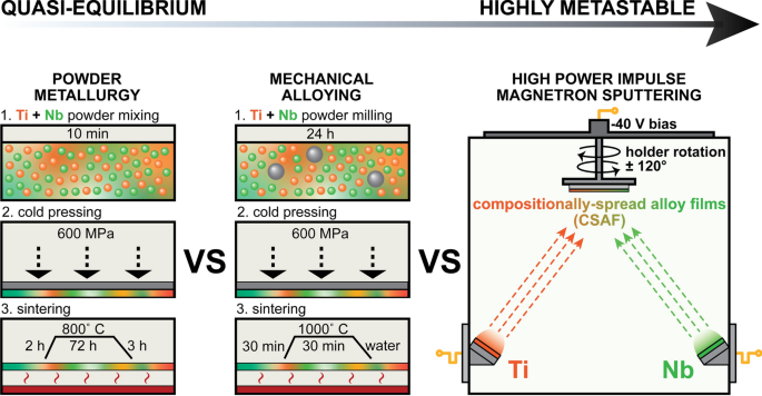
Hardening and Strengthening Effects Induced by Incorporation of Titanium in Hexagonal Boron Nitride Ceramics

Laser Powder Bed Fusion Printing of CoCrFeMnNi High Entropy Alloy: Processing, Microstructure, and Mechanical Properties

Magnetic and Microstructural Properties of Nanostructured/Amorphous NiTi Prepared by Mechanical Alloying

Avoid common mistakes on your manuscript.

Introduction

Titanium and its alloys are commonly used for medical applications, mainly as hard tissue implants. Their properties include high biocompatibility, corrosion resistance in body fluids, osseointegration, low Young’s modulus compared to other metallic biomaterials, and high relative strength [ 1 , 2 , 3 , 4 ]. Alloying Ti to increase the yield strength through the formation of dual-phases containing α and β structures led to the development of the Ti6Al4V (wt%) alloy [ 5 ]. However, despite obtaining improved mechanical properties, further research is required to overcome important issues related to Ti6Al4V. One major objective is to replace toxic Al and V by more biocompatible metals [ 6 ]. Another concern is the relatively high difference in Young’s modulus of the alloy (110 GPa) and bone (10–30 GPa), which is expected to generate stress shielding effects [ 7 , 8 ]. One possibility of addressing these issues is using other β-stabilising elements, such as Nb, Zr, Mo and Ta, which tend to decrease the β transus temperature [ 9 , 10 ]. Using Nb as a β -stabiliser is interesting, due to its significant impact on the α-β transformation temperature with only α and β being present in the stable phase diagram, while additionally allowing to decrease Ti’s Young’s modulus [ 11 , 12 , 13 ]. Furthermore, Ti-Nb alloys are non-cytotoxic and corrosion resistant in intravenous fluids [ 14 , 15 ]. However, it should be noted that in the metastable phase diagram it is possible to observe other phases, such as Ti-based martensites, i.e. αʹ, αʹʹ or ω, which might be crucial in understanding the possibilities of forming many other phases using non-equilibrium manufacturing methods. Furthermore, the metastable Ti-Nb phase diagram exhibits the monotectoid transformation, which results in the formation of two body-centred cubic Ti-based solutions with different Nb contents, namely β 1 and β 2 . This phenomenon is known as spinodal decomposition, where two phases with similar crystal structures but different compositions are formed due to different electron to atom ratios. The mechanical properties of alloys can be affected by the presence of this effect. The formation of β 1 and β 2 phases in alloys is critical to engineering material properties and can be controlled by manufacturing conditions and post-processing by annealing [ 16 ]. During the formation of Ti-Nb alloys, Ishiguro et al . [ 17 ] observed the presence of bcc-separated phases, specifically β 1 and β 2 . This type of phase separation is also common in other stable phase diagrams, such as the Ti-Mo phase diagram [ 18 ]. Figure 1 presents the Ti-Nb phase diagram as a function of Nb contents and temperature [ 19 , 20 ].

a Metastable Ti-Nb phase diagram, b diagram with the temperature curve for martensite (αʹ and αʹʹ)—Ms and ω transformation start, as a function of Nb contents and temperature [ 19 , 20 ].

Other than conventional powder metallurgy (PM), mechanical alloying (MA) can be employed for non-equilibrium processing, which involves repeated cold welding, fracturing, and rewelding of the powder. This leads to the production of ultrafine-grained or nanocrystalline materials and enables producing non-conventional materials in the form of nanocomposites, with uniform ceramic phase dispersions in a metallic matrix. Furthermore, it allows to fabricate many non-equilibrium phases, e.g. supersaturated solutions, metastable and quasi-crystalline intermetallic phases or amorphous phases [ 21 ].

Zhuravleva et al. [ 22 ] and Kalita et al. [ 23 ] used a high-energy planetary ball mill to perform mechanical alloying for the fabrication of Ti-Nb alloys, specifically Ti26Nb (at.%) and TixNb (14 < x < 26 at.%, where TixNb refers to a Ti alloy containing x % of Nb). Both studies observed the formation of β-type Ti26Nb with crystallite sizes of approx. 12 nm. Bulk samples were obtained through spark plasma sintering with a compressive yield strength ranging from 650 to 950 MPa at 0.5% porosity. In a comparative study on the fabrication of Ti-Nb binary alloys for biomedical applications, Karre et al . [ 24 ] compared the consolidation of mixed Ti-xNb (x = 18.75, 25, and 31.25 at.%) powders using spark plasma sintering and conventional cold pressing and pressureless sintering. The resulting samples contained both β-phase and α″. The alloys produced in this study have a Young’s modulus of around 90 GPa and are non-toxic to osteoblast-like cells.

Wang et al . [ 25 ] conducted a comprehensive analysis of Ti35Nb (wt%) produced by selective laser melting, investigating their microstructure, mechanical properties and corrosion resistance. The study examined the material’s microstructure, mechanical properties, and corrosion resistance. The results confirmed that the material exhibits improved corrosion resistance compared to commercially pure titanium. This was demonstrated through open-circuit potential, potentiodynamic, and EIS Nyquist experiments, indicating its suitability for biomedical applications. Heat treatment can enhance the corrosion resistance of Ti35Nb alloys, leading to better homogenization of alloys made with mechanically mixed titanium and niobium powders. The authors also observed a positive effect when using gas atomized ingots as the powder feedstock [ 26 ]. Samples made with gas atomized pre-alloyed powders showed even greater homogeneity, increased ductility, and a lower modulus of approximately 72 GPa. Furthermore, alloys produced using this method did not contain any unmelted Nb particles. Unmelted Nb particles have been shown to significantly affect the mechanical properties of selectively laser-melted Ti-Nb alloys, particularly their Young’s modulus, contributing to an overall increase [ 27 ].

The main aim of this research is to gain a comprehensive understanding of the Ti-Nb phase diagram using different fabrication methods that operate under distinct thermodynamic non-equilibrium conditions. The Ti-Nb binary system was analysed using three manufacturing techniques: powder metallurgy, mechanical alloying, and high power impulse magnetron sputtering (HiPIMS). HiPIMS was used to create compositionally spread alloy films (CSAFs), with the purpose of screening materials and observe trends in material properties, such as crystal structure, hardness, and Young’s modulus, across different elemental compositions. The CSAFs supported the discovery and analysis of phase transformations in various materials and provided insights for bulk sample fabrication [ 28 , 29 , 30 , 31 , 32 , 33 ]. Previous research on Ti-Nb alloys, using direct-current magnetron sputtering (DCMS), showed that alloys containing 15–40% Nb achieved a single-phase β-structure [ 34 ]. The films produced exhibited varying grain structures depending on the material’s composition, including layer-island, columnar, or V-shaped structures. HiPIMS resulted in higher ion/neutral flux ratios impacting the substrate’s surface, leading to denser and more textured films with increased potential and kinetic energies compared to DCMS [ 35 , 36 , 37 , 38 , 39 , 40 , 41 , 42 , 43 , 44 , 45 ]. Investigations were conducted to elucidate the influence of energy considerations and alloying mechanisms on phase formation, lattice constant variations, and mechanical properties in these processes. This comprehensive understanding enables the development of predictive models for the behaviour of Ti-Nb alloys produced by MA, potentially paving the way for their application as a new generation of dental implant materials. Furthermore, this work provides valuable insights that can be applied to broader areas of materials engineering. It is particularly useful for studying complex systems, such as ternary and quaternary systems, which are difficult to explore using traditional bulk technologies. This research has the potential to advance materials science in various fields, such as aerospace, tooling, and functional materials, where it is crucial to evaluate the effects of different dopants on specific chemical and physical properties.

Set-up and sample production

Ti-Nb alloys were produced using three different techniques: conventional powder metallurgy and mechanical alloying (PM_TiXNb and MA_TiXNb, where X = 10, 20, 30) for fabricating bulk samples, and HiPIMS (TF_TiXNb) for obtaining gradient films. The Nb contents range of interest is between 10 and 30 at.%, as at these concentrations the transition of the Ti alloy to a pure cubic structure is expected. Only atomic percentage will be used in this work to indicate alloy composition, unless otherwise specified.

Sample preparation

Bulk Ti-Nb alloys were produced using Ti (Alfa Aesar, 325 mesh, 99.9% purity, CAS:7440-32-6) and Nb (Sigma-Aldrich, 325 mesh, 99.8% purity, CAS:7446-03-1) powders. The morphology of the precursor powders can be found in our previous paper [ 46 ]. For PM, the powders were mixed for 10 min to homogenise their distribution and were then cold pressed at 600 MPa. During sintering, the temperature was gradually increased to 800 °C over a period of 2 h, maintained for 72 h and finally reduced to room temperature within 3 h. The process of sintering was performed under a protective Ar atmosphere in quartz tubes.

For MA, the powders were transferred to vials in a protective Ar atmosphere (O 2 < 2 ppm and H 2 O < 1 ppm) inside a glove box (LabMaster 130, MBraun) and subjected to milling for 24 h using a SPEX 8000 Mixer Mill (SPEX® Sample Prep), which is particularly suited for alloying screening processes [ 21 ]. The milled powders were consolidated by cold-pressing (600 MPa) and sintering (30 min heating until reaching 1000 °C, 30 min holding, and then water cooling). The entire process was kept under a protective Ar environment within sealed quartz tubes. The sintering temperature of the mechanically alloyed samples was chosen based on the group’s previous work [ 47 ], where it was confirmed on the example of binary Ti-Mo alloys that higher sintering temperatures efficiently promote the formation of β.

The temperature applied during conventional PM sintering was lower than that used for MA-prepared powders to reduce the possibility of oxidation while the powders were held at elevated temperatures over a three-day period.

The composition of the final bulk samples was measured using X-ray fluorescence (XRF) spectrometry and was similar to the composition of the powders (Table 1 ). The Fischerscope X-Ray XDV-SDD X-Ray fluorescence spectrometer (Fischer Technology Inc.) was used for composition and film thickness measurements. The instrument was set to a voltage of 50 kV, collimator size of 0.3 mm, primary filter of Ni, spot size of 0.33 mm, and a measurement time of 30 s. For film measurements, the content gradient over the measurement spot size can be neglected. For bulk samples, five measurements were conducted for each compositional value. It should be noted that the composition uncertainty of the PM samples is greater than for MA, caused by coarse-grained structure formation during PM, leading to a more varied chemical composition at the microscale than for ultrafine-grained samples obtained via MA.

CSAF samples were deposited via HiPIMS (Hipster 1, Ionautics) in an in-house modified HexL reactor (Korvus), described in previous works [ 48 , 49 ]. Pure Ti (99.995% purity) and Nb (99.95% purity) disc 2” × 0.1252” targets (Kurt J. Lesker) were installed onto 2 unbalanced magnetrons (Korvus). The films were deposited onto < 100 > -oriented silicon wafers (MicroChemicals). An in situ pre-treatment step was used to remove the native Si oxide layer by exposing the wafers to a microwave (MW) plasma produced by 3 MW plasma sources (Aura-wave, SAIREM) [ 48 , 49 , 50 , 51 ]. A pulse width of 25 µs was selected for both the Ti and Nb targets, with the sputtering process run in constant peak current mode (see Fig. S1 in Supplementary Materials). The pulse frequency was adapted to modify the deposition rates and film composition. Four samples were selected for these investigations: TF_Ti < 40Nb (overview sample covering the entire range of interest from 3 to 30% Nb, produced using two magnetrons installed face-to-face), and 3 samples targeting Nb concentrations of 10, 20 and 30% (produced using three magnetrons, two Ti and one Nb). The composition spread over the wafer was adjusted by rotating the substrate holder by ± 120° with a period of approximately 15 s. The substrate bias was set to − 40 V and Ar pressure to 0.6 Pa. The HiPIMS process was operated in constant peak current mode. The total thickness of the TF_Ti10Nb, TF_Ti20Nb, and TF_Ti30Nb films varied between 0.8 and 1.3 µm. The alloy concentration ranges are given in Table 2 .

Characterisation methods

The film cross section was imaged using a Hitachi S-4800 high-resolution cold field emission (CFE) scanning electron microscope (SEM) (Hitachi High-Tech Corporation). Additionally, the structure of conventionally produced Ti-Nb alloys was observed using optical microscopy (Olympus GX51, JPN) after etching in Kroll reagent. The structure of the bulk samples was evaluated via electron backscatter diffraction (EBSD) using a Tescan Mira microscope (Tescan) and Digiview V camera (EDAX).

A Bruker D8 Discover X-Ray diffractometer (Bruker) with CuKα radiation was used for crystal structure evaluation of the film and bulk samples at room temperature using the following parameters: 40 kV voltage, 40 mA anode current, 30–80° 2θ range, with a 0.0196° step size. For the films, a greater time per step was set than for the bulk samples (1 vs 0.5 s/step) as a smaller slit and, in turn, spot size was used.

High Score Plus software (Malvern Panalytical B.V.) was used to perform Rietveld refinement. This is a profile fitting procedure that utilises diffraction patterns obtained from X-ray diffraction databases, such as the International Centre for Diffraction Data (ICDD) PDF4 + , as described in these articles [ 52 , 53 ]. The Rietveld refinement procedure refines the background, profile coefficients, lattice parameters, linear absorption coefficients, and other variables in a least squares procedure to ensure the calculated pattern best fits the experimental data. Each phase’s data is calculated separately, and their relations are used to calculate the phase fractions, which are mainly directly related to the calculated scale factor (proportionality correction) [ 54 , 55 ]. Phase fraction calculations are only performed for bulk samples that are randomly oriented due to the significant uncertainties introduced by preferred orientation. The provided data for films are limited to lattice constants.

A 1.5° offset from the symmetrical diffraction geometry was introduced to the films to avoid the signal from the Si substrate. For film samples showing a significant contents gradient, the samples were aligned on the sample stage in such a way that the contents gradient over the measurement spot size was as small as possible.

The hardness and Young’s modulus of the films were measured using a Hysitron Ubi Nanoindenter (Bruker) equipped with a diamond Berkovich indenter tip. A load force of 2 mN was used to achieve an indentation depth of approximately 10% of the films’ thickness. The Oliver-Pharr method was used to analyse the load–displacement data [ 56 ]. Young’s modulus was calculated from the reduced elastic modulus using a Poisson ratio of 0.32 [ 57 ]. The loading and unloading times were 10 s long, and the force was held for 5 s. Before the measurement, the tip area function was calibrated using fused silica as the reference sample. The mechanical properties of the bulk samples were examined by applying a higher force of 300 mN, loading time of 20 s and creep time of 5 s. The effect of porosity on the mechanical properties was neglectable, as the indents of approx. 1.5–2.5 μm were made in areas free of pores. A Fischerscope HM2000 nanoindenter (Fischer Technology Inc., USA) equipped with a Vickers tip was used for testing the bulk samples.

Structural analysis

The X-ray diffractograms of the PM_TiXNb samples (Fig. 2 ) revealed that the crystal structure of all produced alloys consisted of two phases: hexagonal close-packed (hcp) α and body-centred cubic (bcc) β. The contents (mass fraction) of β increased from 46% for Ti10Nb to 91% for T30Nb. The unit cell volume of the bcc β phase was equal to 35.7(1) Å 3 for alloys PM_Ti10Nb and PM_Ti20Nb and 35.6(1) Å 3 for PM_Ti30Nb. Assuming that the α phase contains 2% Nb (the maximum solubility limit of Nb in α at 500 °C based on the stable Ti-Nb diagram [ 20 ]), the resulting β phase composition is Ti21Nb, Ti24Nb, and Ti34Nb. This implies that the Nb contents in β varies much less than its overall contents in the produced samples. The porosity of the PM_TiXNb samples varied between 2.0 and 2.9 vol. %, as calculated based on light microscopy images using the ImageJ software (see Fig. S2 in Supplementary Materials). Optical microscopy assessment of the chemically etched samples confirmed a mean grain size of 10 μm for both the α and β phases across all three compositions (refer to Fig. S3 in Supplementary Materials).

Diffractograms of the PM samples. Mass fractions of identified phases, determined using Rietveld method, are given above the corresponding diffractograms (uncertainties given in brackets).

Figure 3 displays the evolution of the crystalline structure of the MA_TiXNB powder with increasing milling time. After 15 min of milling, the XRD revealed the presence of α and Nb-rich phases. The diffraction peaks of these phases were visible at early milling stages and their ratio depends on the composition of the powders. During milling, the β phase appeared at the expense of both Nb and α phases. For powders with a relatively high Nb contents (MA_Ti20Nb, MA_Ti30Nb) the β phase started to dominate. After 24 h of MA, both samples became single-phase β-structured alloys. The MA_Ti10Nb powder, however, had a α/β dual-phase structuring even after 24 h of milling. The amount of β phase in this material did not change significantly between 6 and 24 h of milling. However, significant peak broadening of both phases occurred.

Diffractograms of the a MA_Ti10Nb, b MA_Ti20Nb, c MA_Ti30Nb alloys mechanically alloyed for different durations.

Next, the MA powders were sintered at 1000 °C [ 47 , 58 ] and analysed via XRD (Fig. 4 ). The sintered samples contained α and β phases (MA_Ti20Nb and MA_Ti30Nb), as well as an additional orthorhombic Cmcm α″ phase in the case of the Ti10Nb alloy. Therefore, sintering led to the formation of α in alloys MA_Ti20Nb and MA_Ti30Nb (not present in the previously analysed MA powders). The formation of the Cmcm α″ phase, present in the low Nb contents alloy, might be favoured by the fast cooling of the samples in water. The contents of the β phase were observed to strongly increase with increasing Nb contents, i.e. from 20% in MA_Ti10Nb to almost 100% in MA_Ti30Nb.

Diffractogram comparison between the milled (24 h) powders and specimens produced from those powders after sintering at 1000 °C, for all three investigated samples (uncertainties given in brackets).

Figure 5 shows the evolution of the bcc β phase’s unit cell volume during the various steps of MA (milling duration, sintering). The unit cell volume was determined using Rietveld refinement using the diffractograms presented in Figs. 3 and 4 . The uncertainties are based on the differences in the used numerical models for the same data set and do not include the effects of reproducibility of the milling process and XRD measurements.

Evolution of the unit cell volume of the bcc Nb/β phase in Ti10Nb, Ti20Nb, Ti30Nb with milling time and comparison with the bulk sample cold pressed and sintered at 1000 °C (CP + S), Rietveld refinement (uncertainties given in brackets).

The volume of the unit cell decreased with increasing milling time up to 10 h, independent of the Nb contents. After 24 h, the unit cell volume for alloy powders containing 10 and 20% Nb did not show a significant reduction, however, for Ti30Nb it continued to reduce almost linearly in time to 35.1 Å 3 . During the last production steps (cold pressing and sintering) the unit cell volume decreased again for all MA samples. A clear trend can be seen for different Nb concentrations, decreasing from 35.6 Å 3 for the MA_Ti10Nb sample to 34.1 Å 3 for the MA_Ti30Nb one. EBSD was used to confirm the phase structure of the MA_Ti30Nb sample after milling and sintering (Fig. 6 ). The sample contained 95% β and approx. 5% α. The grain size distribution for both phases is relatively large, with an average grain size of 500 nm for α and 1.2 µm for β, respectively, with a standard deviation of approximately 50% of the averaged values for both. This proves that MA_Ti30Nb is an ultrafine-grained material, which normally would not be achievable through arc-melting or conventional powder metallurgy. The porosity of the MA_TiXNb samples (ranging from 18.6 to 26.4 vol. %, as shown in Fig. S2 in Supplementary Materials) was significantly higher than that of the PM_TiXNb samples. This was due to the lower compaction of MA_Ti20Nb, which resulted from the increased tendency of powder particles to weld during mechanical alloying, forming larger agglomerates. It is unclear to the authors why the cold welding phenomenon was more intense in Ti20Nb alloys compared to Ti10Nb and Ti30Nb. Sample MA_Ti20Nb had the highest porosity of all the samples, with an overall porosity of 26.4%. The pores are larger and connect to form channels compared to the other samples. Additionally, the pre-sintered agglomerated particles are visible in the sample’s microstructure, along with the necks formed in the contact area between them.

EBSD analysis of cold pressed and sintered at 1000 °C MA Ti30Nb alloy a crystal orientation maps of α and β phases. The IPF colour is displayed for the z-direction (cold pressing axis); b α and β phase distribution map. The crystal orientation maps were acquired using electron beam conditions of 20 kV and 10 nA, with a 100 nm step size.

XRF mapping was performed to determine the thickness and composition gradient across the deposited film. Afterwards, the wafer was cleaved and an example fracture cross section of the HiPIMS-produced film is presented in Fig. 7 . It can be seen that the film is highly compact with no visible columns, in contrast to what has been reported for DCMS [ 59 ].

Example fracture cross section of the binary Ti-Nb film, SEM-SE.

The obtained diffractograms revealed that the films are all highly textured. The intensities of the peaks coming from the (110) lattice plane are much more intense compared to others. The XRD analysis of the TF_Ti < 40Nb sample (large concentration spread) shows clear trends in the formation of different phases with varying Nb contents. Figure 8 summarises the XRD diffraction angle scans performed at different wafer positions, mainly along the border between the extremes of the concentration range. For Nb concentrations of 3–30%, it is possible to distinguish four different peaks in the 2θ range of 34–40°. These peaks are attributed to 3 different phases: (1) Peaks at 34.9 and 38.3° are linked to the α hcp P63/mmc lattices (010) and (002), respectively, (2) The peak at 38.8° for Nb contents of 3% shifting to lower angles with increasing Nb contents is attributed to the β 2 cubic body-centred Im-3 m lattice (110), and (3) the fourth peak, visible for a Nb contents > 12%, which shifts to higher angles with increasing Nb contents, cannot be unambiguously attributed to a known phase of the Ti-Nb system, however, it is labelled as β 1 throughout the text. The peaks of different planes belonging to α, β 1, or β 2 were not observed in the diffractograms of the film alloys due to their highly textured structure. The oxygen contents for the produced materials are predicted to be < 5 at.% as in other studies, where HiPIMS was used for producing Ti-based films [ 60 , 61 ]. Films with Nb concentrations < 10% contained α and β 2 phases, i.e. a small amount of Nb is solute in α and the rest forms a separate β 2 phase. Following the Nb gradient from 3 to 10%, the peak positions did not shift, however, their relative intensities changed in favour of the β 2 peak. At approx. 10% Nb, the intensities of the α peaks at 34.9° (010) and 38.3° (002) significantly drop, giving rise to a new reflex initially observed at 35.7°, which the authors have attributed to β 1 (110). As the deposited films are highly textured, attribution based solely on XRD is questionable. The authors have adopted this interpretation, as with increasing Nb contents, the two peaks continuously move to a single peak, attributed to β. When looking into areas of increasingly high Nb contents, the two reflexes shift and move together, i.e. the β 1 (110) phase shifts to larger angles, whereas the β 2 peaks move to smaller angles to finally form a single peak for an approx. Nb contents of 30%.

Diffractograms of the TF_Ti < 40Nb film between 3 and 30% Nb, the uncertainty in the Y-range is 1%.

Based on the observed peak positions and under the assumption that both peaks belong to a bcc structure, the evolution of the unit cell volume was determined as a function of increasing Nb contents in the TF_Ti < 40Nb film (Fig. 9 ) via Rietveld refinement.

Changes in unit cell volume of the bcc β 2 and β 1 phases as a function of Nb contents in the Ti-Nb 3-30 CSAF, Rietveld refinement.

The unit cell volumes of β 1 and β 2 are influenced by the Nb contents. The unit cell volume of the β 2 phase remained stable at 36.7 Å 3 , with some fluctuations for Nb concentrations below 10% (still possible to identify α, however, not yet β 1 ). Above this Nb contents (α replaced by β 1 ) the unit cell volume increased to reach a local maximum of 37.7 Å 3 for 19% Nb to then slowly drop to a value of 37.1 Å 3 . The unit cell of the β 1 phase, which replaced α for Nb concentrations > 8%, first shrunk rapidly from 48.4 to 41.1 Å 3 at a Nb contents of 19% to slowly drop until β 2 and β 1 became indistinguishable at a Nb contents of 28%. Figure 10 shows a detailed X-ray diffractogram obtained from different spots on the wafer, all exhibiting the same chemical composition of Ti23Nb. The Nb contents variation was less than 2%, however, the mean energy and angle of incidence of the film-forming particles differed, as the relative position of the spots to the magnetron sources was not the same. The position of the peak attributed to the (110) plane of β 1 and β 2 is the same for all measured regions, however, their relative contribution changed considerably between 46 and 90% β 2 . It can be summarised that the unit cell volume of the two phases depends only on the relative amount of Nb incorporated into the film, whereas the relative phase distribution depends on the detailed changes of the deposition environment.

Detailed X-ray diffractogram overview acquired from different locations on the TF_Ti30Nb sample corresponding to the same chemical composition of Ti23(2)Nb, the relative contribution of the β 2 is given in the legend (top left corner).

Mechanical properties

The mechanical properties of the PM (PM_TixNb) and MA (MA_TiXNb) bulk samples are summarised in Fig. 11 a. For the PM samples, both the materials’ hardness and Young’s modulus decreased with increasing Nb contents, from approx. 4 to 1.5 and 125 to 85 GPa, respectively. The elastic modulus for MA_Ti10Nb of 99 GPa is significantly lower than the 141 GPa of commercially pure titanium (cp Ti) Grade 2 [ 46 ]. The further decrease in both elastic modulus and hardness was observed for MA_Ti20Nb, making the trend similar to that of the PM bulk samples. However, the MA_Ti30Nb alloy exhibited a reversed trend to MA_Ti20Nb, i.e. both the hardness and elastic modulus increased.

Hardness and elastic modulus of a PM and MA bulk samples, b film samples with varying Nb contents, c Ti23Nb regions measured on the TF_Ti30Nb sample as a function of β 2 contribution.

Nanoindentation was performed on the film samples (Fig. 11 b), where their thickness was ≥ 1 µm to avoid substrate influences. The stated Nb contents may vary by 2% due to sample positioning in the nanoindenter, as the uncertainties in the content differences measured on a single wafer are significantly smaller. For pure Ti deposited in the same manner as the alloys, the hardness and elastic modulus were measured to be approx. 3.9(8) GPa and 153(16) GPa, respectively. For Nb concentrations up to 20%, the hardness increased to approx. 4.8 GPa, whereas a drop in hardness was observed for samples containing 26% Nb (3.1(1) GPa) and 31% Nb (3.4(1) GPa). The Young’s modulus did not vary significantly (between 110 and 138 GPa) and did not follow any specific trends. However, the measured values were lower than for pure Ti. The higher modulus values were, however, generally attained for lower Nb concentrations, when the α phase was still present.

The mechanical properties of the Ti23Nb regions on the TF_Ti30Nb sample, which show a strong variation in the β 2 phase distribution (Fig. 10 ), are shown in Fig. 11 c. The hardness of this material increased with increasing β 2 contribution from 3.6 to 4.8 GPa. Simultaneously, the elastic modulus increased from 110 to 125 GPa, however, more result scattering occurred. For the thin film samples, as shown in Figs. 11 b and c, the mechanical properties depend on the phase composition, particularly the β 2 contribution, rather than the Nb content once α disappears.

Energy considerations and alloy formation mechanisms in diverse production methods

Ti-Nb alloys with similar chemical compositions but manufactured using different methods were studied. The PM approach involves low-energy processes. The involved energy during cold pressing at 600 MPa is below the meV range and can therefore be considered negligible. Sintering at 800 °C requires thermal energies of 0.1 eV, which is approximately two thirds of the enthalpy of fusion. Aguilar et al . [ 62 ] estimated the Gibbs free energy for fabrication by means of MA to be in the range of 5–10 kJ mol −1 , corresponding to 0.1 eV at the atomic level. The process of mechanical alloying increases the free Gibbs energy above the mixing energy, which alters the solubility limits through the formation of high-density defects. This study demonstrates that refining crystallites has a greater impact on solubility changes than elastic strain energy caused by a high dislocation density. This highlights the benefits of using mechanical alloying as a preferred technology for powder preparation. However, the technique has a disadvantage in that the produced samples have increased porosities compared to those produced with conventional powder metallurgy. Nevertheless, as previously stated, the MA samples could be further optimised by applying additional consolidation techniques, which would significantly reduce their porosity. Manufacturing Ti-Nb through magnetron sputtering, particularly HiPIMS, involves significantly higher energies. Ions participating in film growth accelerate in the plasma sheath. The energy of the particles can be estimated using the bias voltage, which in this study was −40 V. Due to particle collisions on the way to the substrate (with a mean free path of 13 mm for Ar at 0.5 Pa and room temperature), the average energy will be slightly lower. Additionally, the ions carry potential energy, specifically ionisation energy [ 63 , 64 ].

Alternatively, we can compare these fabrication methods based on their main alloy formation mechanisms. PM relies mainly on diffusion between Ti and Nb grains during sintering, with negligible contribution from applied pressure. On the other hand, both MA and magnetron sputtering offer additional formation mechanisms. The milling process liberates considerable friction energy, which strongly deforms and reduces the grain size to 20–30 nm in diameter [ 46 ]. Defect generation, grain size reduction and forced Nb integration mostly destroy the α phase dominant in the pure Ti precursor powder during milling. These conditions favour the formation of the alloy phase. The high surface-to-volume ratio of the powder increases the interaction zone between the grains during cold pressing and sintering, compared to the PM approach using relatively large grains. The process of forming alloys through film fabrication differs significantly from the two bulk techniques. Magnetron sputtering transfers the target material in the form of a cloud consisting of single atoms and ions, without retaining any memory of the target’s crystalline structure. Each pulse under the HiPIMS conditions contributed to less than one atomic layer. The species that hit the surface and participate in film growth exhibit a wide energy range, from thermal energy to a few tens of electron volts. The more energetic particles transfer their energy to the growing crystals through multiple collisions, allowing for crystal re-arrangements and surface mobility [ 65 , 66 , 67 ].

The impact of niobium on phase formation and lattice constant variation

The amount of Nb required to achieve β-stabilisation varies depending on the process mechanism. It is highest in the case of PM methods and lowest when using HiPIMS. The proportion of cubic β in the phase composition is significantly greater in the MA materials compared to PM. This is due to the additional energy stored in the milled materials, which favours the formation of β over α. While the authors have not explicitly stated this, there is potential for enhancing material properties by utilising other advanced synthesis techniques, such as spark plasma sintering (SPS). According to existing literature, SPS can enhance mechanical properties by creating materials with a more refined microstructure [ 68 , 69 ]. However, scalability presents a significant challenge, particularly when scaling up to discs larger than 10 cm in diameter [ 70 , 71 ]. In the range of 20–30% Nb, the phase structure of the MA samples consists of hcp α and bcc β. However, the phase composition of the HiPIMS films in the same Nb content range does not contain any hcp α. The phase structure analysis revealed metastable phases in both the HiPIMS and MA samples. The HiPIMS samples contained separated bcc phases: β 1 and β 2 , while the MA samples contained orthorhombic Cmcm α”. These are a consequence of non-equilibrium mechanisms. Other authors have confirmed the structural evolution in multiple phases using DCMS as a composition spread alloy thin film. This aligns with the results observed in the fabrication of alloys through pressureless sintering of mechanically alloyed samples [ 72 ]. The combined effect of efficient precursor material mixing and non-equilibrium conditions favours the rapid transformation of α into metastable a” and β. The PM samples only contained stable α and β.

The analysis indicates that the lattice constant of β remains unaltered by the Nb content in conventional microcrystalline alloys. However, in the case of the MA samples, an increase in the amount of Nb solute in the Ti lattice results in a reduction in the unit cell volume, as illustrated in Fig. 5 . The transition process from α to β stops once all available Nb is consumed during the first 10 h. However, a significant amount of free Nb remained in the case of MA_Ti30Nb powder. The authors are uncertain as to why the reduction in unit cell volume ceased at the same level for both MA_Ti10Nb and MA_Ti20Nb after 10 h, despite the latter having a higher amount of free Nb. Furthermore, peak broadening was observed in both the α and β phases during mechanical alloying. This corresponds to structure fracturing caused by high energy impact during milling and the associated increase in the number of crystal defects, leading to the powders’ hardening during milling [ 73 ]. The literature on mechanical alloying technologies, such as [ 74 ], has extensively discussed peak broadening and defect formation. The defects found in the analysed powder particles include dislocations, vacancies, stacking faults, and increased grain boundaries. In addition, the formation of crystal defects with a high density can result in the amorphisation of mechanically alloyed powders. Mechanical alloying involves the simultaneous occurrence of cold welding and fracturing phenomena. The process generates high mechanical energy due to multiple collisions between milling balls and powder particles, resulting in particle deformation and fracturing. Cold welding is particularly dominant in the initial stages of the process. The agglomeration of powder particles is promoted by friction, which facilitates mechanically-activated diffusion. Furthermore, the process of cold pressing and sintering resulted in a reduction of the unit cell volume. This phenomenon was attributed to the diffusion of Nb into the β lattice and possibly thermal relaxation.

An increase in Nb content in the film samples, particularly in β 1 , results in a significant reduction of the unit cell volume. The unit cell volume decreased from 48.4 Å 3 for the alloy containing approximately 8% Nb content to 37.1 Å 3 for 30% Nb content and single-phase structuring. Conversely, the unit cell volume of β 2 increased from 35.7 Å 3 for low Nb to 37.1 Å 3 for high Nb. The value is similar to the literature values found for both pure Nb (36.1 Å 3 ) [ 75 ] and Ti (ranging from 35.4 Å 3 [ 76 ] to 36.2 Å 3 [ 77 ]). The unit cell volume of the alloy β 2 , observed along with α, does not change significantly with increasing Nb contents. The increase in unit cell volume only occurs once α has disappeared and β 1 is clearly visible. The β 2 phase may be due to a Nb-rich phase that incorporates the Nb atoms reaching the α-dominant surface. However, the authors could not provide evidence for this hypothesis. Additionally, the deposited films showed greater texturing than the bulk samples, with randomly oriented grains. The film texturing hindered accurate crystal structure analysis. The texture and microstructure of the film are influenced by the competition between surface and strain energy and can vary with film thickness. For example, TiN texture can change from the (200) plane to the (111) plane as thickness increases, while Ti films change their orientation from (100) to (002). Additionally, (101) plane texture results from thermal stress in DC magnetron sputtered titanium [ 43 , 65 , 66 , 67 , 78 , 79 ]. Figure 12 schematically shows the phase distribution and domain formation during film deposition.

Schematic distribution of phases in gradient films produced via HiPIMS for a TiNb alloys < 10% Nb, b TiNb alloys > 10 and < 30% Nb c Ti30Nb alloy.

Impact of Nb on the mechanical properties of Ti-Nb alloys

Regardless of the production method, nanoindentation results show that the addition of Nb, which acts as a β-stabiliser, reduces the Young’s modulus of the alloys in comparison to pure Ti. The correlation between Nb content, hardness, and Young’s modulus observed in this study is consistent with the findings of other researchers [ 13 , 80 , 81 ]. The hardness and elastic modulus of the MA samples decreased with only a 10% Nb concentration due to the formation of a triple-phase structure consisting of α″, β and α. The reduction between MA_Ti10Nb and MA_Ti20Nb is due to the transition from a triple-phase structure (with α and α″ contents of approximately 80%) to a dual-phase structure with a dominant β content of approximately 91%. Tan et al . [ 80 ] produced alloys using a conventional casting technique to create TixNb4Zr alloys (x = 14, 17, 20). They observed the formation of two different phase structures in the materials produced: α′ + α″ + β + ω and β + α″. These structures significantly influenced the properties of the alloys. The Young’s modulus decreased from approximately 36 GPa to 29 GPa as the content of β phase increased and the content of α′ + α″ + ω phases decreased with Nb content. The decrease in modulus is explained by two factors: (1) An increase in α” phase content during the expansion of α΄ and α” phase, and (2) The dominance of β phase in the Ti20Nb4Zr alloy structure. This effect of Nb content on hardness and Young’s modulus has also been observed in other alloys, such as TixNb6Fe (x from 0 to 6) [ 13 ], where the Young’s modulus was lower than that of all PM_TixNb, MA_TixNb, and TF_TixNb alloys. Ehtemam-Haghighi et al . [ 81 ] found comparable correlations between the structure, composition, and mechanical properties of alloys stabilised by other elements, such as Fe and Ta. The alloys’ structures comprise of the α″ and β phases, with the Ti9Fe3Ta alloy having the highest content. This alloy exhibits mechanical properties, such as a hardness of 3.4 GPa and a Young’s modulus of 93 GPa, similar to those in the current work.

It is important to note that PM_30Nb and MA_Ti20Nb have a similar crystal structure (β content of approximately 91%) and a similar Young modulus of approximately 85 and 96 GPa for the PM and MA samples, respectively. However, their hardnesses differ significantly, with 1.5 GPa for PM_30Nb and 3.2 GPa for MA_Ti20Nb. This difference is due to grain refinement induced via MA, which does not occur during conventional processes [ 82 ]. The lower elastic modulus of sample PM_30Nb may be correlated with its lower hardness compared to the other produced samples. This material is primarily hardened through solid solution hardening without grain boundaries and precipitation strengthening. These three hardening effects affect the mechanical properties of Ti-based alloys [ 83 , 84 ]. Sample MA_Ti30Nb showed an increase in hardness and modulus (to 3.9 and 116 GPa, respectively) with increasing Nb content. The main reason for the increase in Young’s modulus is not yet clear, but it may be related to the microstructure of that particular sample. Additionally, the EBSD distribution maps show a small amount of fine-grained α present in the matrix composed of β, which is atypical (see Fig. 6 ). This could explain the increase in hardness from 3.1 to 3.9 GPa without significant changes in the crystal structure. It is worth noting that the authors did not observe Nb particles with XRD analysis, which have been shown to increase the Young modulus in other research [ 27 ]. Mechanical alloying before sintering offers a significant advantage in producing powders with a single phase Ti-based β-structure. The presence of unmelted Nb particles suggests the need for increased mechanical alloying time, but this issue can be resolved with the application of this technology, as noted in some articles [ 85 ]. Previous research has reported a non-continuous reduction in elastic modulus, similar to what was observed in this study between MA_Ti20Nb and MA_Ti30Nb [ 86 ]. Specifically, the elastic modulus decreased for the Ti5Nb alloy compared to pure titanium (69 GPa), increased for Ti8Nb (88 GPa), and then decreased again for Ti12Nb (77 GPa). However, the elastic modulus of all alloys in these studies, including Ti8Nb, was lower than that of commercially pure titanium (107 GPa).

Due to differences in the method of determining elastic modulus, it is not easy to compare the obtained results with those obtained in the referenced works. This issue was previously highlighted by authors such as Iijima et al . [ 87 ], who attributed the differences to the influence of varying volumes across different testing techniques. The larger measured volume increases the likelihood of the influence of microscopic and macroscopic structural defects on the measured modulus, including defects such as porosity. It is important to note the so-called indentation size effect (ISE), which was studied by Garbiec et al . [ 88 ] and Rodríguez et al . [ 89 ]. These authors have analysed the phenomenon taking into consideration various differences in material properties at the macro-, micro-, and nanoscale. Our research has led to the successful production of alloys with a lower Young’s modulus. For instance, the Ti30Nb30Zr alloy [ 58 ] had a Young’s modulus of 68 GPa, while the Ti23Zr25Nb-45S5 Bioglass composite [ 90 ] and the Ti23Zr25Nb with about 70% porosity functionalised by the addition of 40% ammonium bicarbonate foaming agent [ 90 ] had Young’s moduli of 43 and 56 GPa, respectively. The reduction of the Young modulus was achieved in these studies through the modification of the materials with Zr content, the addition of 45S5 Bioglass bioceramics, and the production of foams with significant porosities.

The hardness and elastic modulus of thin films are affected not only by their chemical composition but also by the deposition parameters and the relative position of the deposition spot to the sputtering targets (see Fig. 11 b and c). The authors have not yet determined the cause of the significant variation in the mechanical properties of the films. No relations between Co-Cr-Ni-Fe film structure and mechanical properties were observed in studies using the Nelson–Riley method and convolutional multiple whole profile (CMWP) analysis [ 91 , 92 ]. Further work is required, including detailed microstructural studies, such as transmission electron microscopy investigations. These investigations will improve our understanding of the spinodal decomposition of the β phase during film deposition, the texture of the films and its effect on the hardness of the materials. In addition, it is necessary to investigate the formation mechanisms of binary systems in other production routes and the differences in nanostructure between the MA_Ti20Nb and MA_Ti30Nb alloys. This would facilitate a more detailed characterisation and comparison in α phase participation between MA_Ti20Nb and MA_Ti30Nb alloys and their effect on the mechanical properties of the alloys produced will also be investigated in detail. It is important to note that the mechanical properties of a material depend on various factors, including grain size and texture, when comparing samples produced by different methods [ 93 , 94 , 95 ]. The produced samples should also be monitored for mechanical behaviour, biological properties, corrosion resistance and microstructure.

This study analysed Ti-Nb alloys produced by three different methods: conventional powder metallurgy (PM), mechanical alloying (MA), and high-power impulse magnetron sputtering (HiPIMS). The analysis and the experiments have led to the following conclusions:

The techniques used for fabrication are crucial in determining the phase compositions and structural evolution of the material. PM relies on grain diffusion, MA increases free energy over mixing energy, while HiPIMS transfers materials as single atoms and ions from a sputtering target.

The manufacturing process is of critical importance in the formation of the β phase in the alloys produced. The samples produced by MA and HiPIMS contain a greater number of metastable phases (β 1 , β 2 and αʹʹ) compared to PM samples. HiPIMS samples contain body-centred cubic β 1 and β 2 phases with high texture and different lattice constants. Conversely, the MA_Ti10Nb sample contains an orthorombic αʹʹ phase. Furthermore, the higher energy stored in the high-density defects of the MA samples resulted in a higher β content compared to the PM samples

The Young’s modulus of the MA samples decreased at Nb concentrations of 10% (100 GPa) and 20% (96 GPa), followed by an increase at a Nb content of 30% (116 GPa). The increase in hardness for MA samples can be attributed to grain refinement. The mechanical properties of the film were found to be correlated with the deposition conditions.

Supplementary information

Supplementary Table S1 and Figs. S1 – S3 include discharge current and voltage traces, HiPIMS deposition parameters, OM micrographs with calculated porosities (P) and OM micrographs of alloys produced via conventional powder metallurgy and etched with Kroll reagent.

Long M, Rack HJ (1998) Titanium alloys in total joint replacement—A materials science perspective. Biomaterials 19:1621–1639

Article CAS PubMed Google Scholar

Elias CN, Lima JHC, Valiev R, Meyers MA (2008) Biomedical applications of titanium and its alloys. Jom 60:46–49. https://doi.org/10.1007/s11837-008-0031-1

Article CAS Google Scholar

Carlsson L, Röstlund T, Albrektsson B et al (1986) Osseointegration of titanium implants. Acta Orthop 57:285–289. https://doi.org/10.3109/17453678608994393

Ratner BD (2001) A Perspective on Titanium Biocompatibility. In: Brunette DM, Tengvall P, Textor M, Thomsen P (eds) Titanium in Medicine. Springer Berlin Heidelberg, Berlin, Heidelberg, pp 1–12. https://doi.org/10.1007/978-3-642-56486-4_1

Chapter Google Scholar

Chen Q, Thouas GA (2015) Metallic implant biomaterials. Mater Sci Eng R Rep 87:1–57. https://doi.org/10.1016/j.mser.2014.10.001

Article Google Scholar

Langley A, Charles TD (2015) Modern metal implant toxicity and anaesthesia. Australasian Anaesthesia 2015:57–65

Google Scholar

Niinomi M (1998) Mechanical properties of biomedical titanium alloys. Mater Sci Eng, A 243:231–236. https://doi.org/10.1016/s0921-5093(97)00806-x

Niinomi M, Nakai M (2011) Titanium-based biomaterials for preventing stress shielding between implant devices and bone. Int J Biomater. https://doi.org/10.1155/2011/836587

Article PubMed PubMed Central Google Scholar

Kuroda D, Niinomi M, Morinaga M et al (1998) Design and mechanical properties of new β type titanium alloys for implant materials. Mater Sci Eng, A 243:244–249. https://doi.org/10.1016/s0921-5093(97)00808-3

Okazaki Y, Ito Y, Kyo K, Tateishi T (1996) Corrosion resistance and corrosion fatigue strength of new titanium alloys for medical implants without V and Al. Mater Sci Eng, A. https://doi.org/10.1016/0921-5093(96)10247-1

Mantani Y, Tajima M (2006) Effect of ageing on internal friction and elastic modulus of Ti-Nb alloys. Mater Sci Eng, A 442:409–413. https://doi.org/10.1016/j.msea.2006.03.124

Chang LL, Wang YD, Ren Y (2016) In-situ investigation of stress-induced martensitic transformation in Ti-Nb binary alloys with low Young’s modulus. Mater Sci Eng A 651:442–448. https://doi.org/10.1016/j.msea.2015.11.005

Ehtemam-Haghighi S, Liu Y, Cao G, Zhang LC (2016) Influence of Nb on the β → α″ martensitic phase transformation and properties of the newly designed Ti-Fe-Nb alloys. Mater Sci Eng, C 60:503–510. https://doi.org/10.1016/j.msec.2015.11.072

Lee CM, Ju CP, Chern Lin JH (2002) Structure-property relationship of cast Ti-Nb alloys. J Oral Rehabil 29:314–322. https://doi.org/10.1046/j.1365-2842.2002.00825.x

Han MK, Kim JY, Hwang MJ et al (2015) Effect of Nb on the microstructure, mechanical properties, corrosion behavior, and cytotoxicity of Ti-Nb alloys. Materials 8:5986–6003. https://doi.org/10.3390/ma8095287

Article CAS PubMed PubMed Central Google Scholar

Xiao X, Yang K, Lei S et al (2023) A β-type titanium alloy with high strength and low elastic modulus achieved by spinodal decomposition. J Alloys Compd 963:171270. https://doi.org/10.1016/j.jallcom.2023.171270

Ishiguro Y, Tsukada Y, Koyama T (2020) Phase-field study of the spinodal decomposition rate of β phase in oxygen-added Ti–Nb alloys. Comput Mater Sci 174:109471. https://doi.org/10.1016/j.commatsci.2019.109471

Murray JL (1981) The Mo-Ti (Molybdenum-Titanium) system. Bull Alloy Phase Diagrams 2:185–192. https://doi.org/10.1007/BF02881476

Banumathy S, Prasad KS, Mandal RK, Singh AK (2011) Effect of thermomechanical processing on evolution of various phases in Ti-Nb alloys. Bull Mater Sci. https://doi.org/10.1007/s12034-011-0338-3

Moffat DL, Kattner UR (1988) Stable and metastable Ti-Nb phase diagrams. Metall Trans A Phys Metall Mater Sci 19:2389–2397. https://doi.org/10.1007/BF02645466

Suryanarayana C (2019) Mechanical alloying: a novel technique to synthesize advanced materials. Research 2019:1–17. https://doi.org/10.34133/2019/4219812

Zhuravleva K, Scudino S, Khoshkhoo MS et al (2013) Mechanical alloying of β-type Ti-Nb for biomedical applications. Adv Eng Mater 15:262–268. https://doi.org/10.1002/adem.201200117

Kalita D, Rogal Ł, Czeppe T et al (2020) Microstructure and mechanical properties of Ti-Nb alloys prepared by mechanical alloying and spark plasma sintering. J Mater Eng Perform 29:1445–1452. https://doi.org/10.1007/s11665-019-04417-0

Karre R, Kodli BK, Rajendran A et al (2019) Comparative study on Ti-Nb binary alloys fabricated through spark plasma sintering and conventional P/M routes for biomedical application. Mater Sci Eng C 94:619–627. https://doi.org/10.1016/j.msec.2018.10.006

Wang JC, Liu YJ, Qin P et al (2019) Selective laser melting of Ti–35Nb composite from elemental powder mixture: microstructure, mechanical behavior and corrosion behavior. Mater Sci Eng: A 760:214–224. https://doi.org/10.1016/j.msea.2019.06.001

Wang JC, Liu YJ, Liang SX et al (2022) Comparison of microstructure and mechanical behavior of Ti-35Nb manufactured by laser powder bed fusion from elemental powder mixture and prealloyed powder. J Mater Sci Technol 105:1–16. https://doi.org/10.1016/j.jmst.2021.07.021

Wang J, Liu Y, Rabadia CD et al (2021) Microstructural homogeneity and mechanical behavior of a selective laser melted Ti-35Nb alloy produced from an elemental powder mixture. J Mater Sci Technol 61:221–233. https://doi.org/10.1016/j.jmst.2020.05.052

Gebhardt T, Music D, Takahashi T, Schneider JM (2012) Combinatorial thin film materials science: from alloy discovery and optimization to alloy design. Thin Solid Films 520:5491–5499

Fleutot B, Miller JB, Gellman AJ (2012) Apparatus for deposition of composition spread alloy films: the rotatable shadow mask. J Vac Sci Technol, A: Vac, Surf Films. https://doi.org/10.1116/1.4766194

Priyadarshini D, Kondratyuk P, Miller JB, Gellman AJ (2012) Compact tool for deposition of composition spread alloy films. J Vac Sci Technol, A: Vac, Surf Films. https://doi.org/10.1116/1.3664078

Selinder TI, Miller DJ, Gray KE et al (1995) Phase formation and microstructure of Nb1 - xAlxN alloy films grown on MgO (001) by reactive sputtering: a new ternary phase. Vacuum. https://doi.org/10.1016/0042-207X(95)00161-1

Potyrailo R, Rajan K, Stoewe K et al (2011) Combinatorial and high-throughput screening of materials libraries: Review of state of the art. ACS Comb Sci 43:579–633

Ludwig A (2019) Discovery of new materials using combinatorial synthesis and high-throughput characterization of thin-film materials libraries combined with computational methods. NPJ Comput Mater 5:70

Gonzalez ED, Afonso CRM, Nascente PAP (2018) Nanostructural characterization of sputter deposited Ti-Nb coatings byautomated crystallographic orientation mapping. Thin Solid Films. https://doi.org/10.1016/j.tsf.2018.06.051

Sarakinos K, Alami J, Konstantinidis S (2010) High power pulsed magnetron sputtering: a review on scientific and engineering state of the art. Surf Coat Technol 204:1661–1684

Gudmundsson JT, Brenning N, Lundin D, Helmersson U (2012) High power impulse magnetron sputtering discharge. J Vac Sci Technol, A: Vac, Surf Films 30:030801. https://doi.org/10.1116/1.3691832

de Monteynard A, Schuster F, Billard A, Sanchette F (2017) Properties of chromium thin films deposited in a hollow cathode magnetron powered by pulsed DC or HiPIMS. Surf Coat Technol 330:241–248. https://doi.org/10.1016/j.surfcoat.2017.10.006

Weichart J, Elghazzali M, Kadlec S, Ehiasarian AP (2009) PVD processes in high aspect ratio features by HIPIMS. In: 52nd Annual technical conference proceedings. Society of Vacuum Coaters. pp 201–206

Barker PM, Lewin E, Patscheider J (2013) Modified high power impulse magnetron sputtering process for increased deposition rate of titanium. J Vac Sci Technol, A: Vac, Surf Films 31:060604. https://doi.org/10.1116/1.4819296

Lewin E, Loch D, Montagne A et al (2013) Comparison of Al-Si-N nanocomposite coatings deposited by HIPIMS and DC magnetron sputtering. Surf Coat Technol 232:680–689. https://doi.org/10.1016/j.surfcoat.2013.06.076

Ait Aissa K, Achour A, Camus J et al (2014) Comparison of the structural properties and residual stress of AlN films deposited by dc magnetron sputtering and high power impulse magnetron sputtering at different working pressures. Thin Solid Films 550:264–267. https://doi.org/10.1016/j.tsf.2013.11.073

Lundin D, Sarakinos K (2012) An introduction to thin film processing using high-power impulse magnetron sputtering. J Mater Res 27:780–792

Jing FJ, Yin TL, Yukimura K et al (2012) Titanium film deposition by high-power impulse magnetron sputtering: influence of pulse duration. Vacuum 86:2114–2119. https://doi.org/10.1016/j.vacuum.2012.06.003

Barker PM, Konstantinidis S, Lewin E et al (2014) An investigation of c-HiPIMS discharges during titanium deposition. Surf Coat Technol 258:631–638. https://doi.org/10.1016/j.surfcoat.2014.08.025

Schmidt S, Czigány Z, Greczynski G et al (2012) Ion mass spectrometry investigations of the discharge during reactive high power pulsed and direct current magnetron sputtering of carbon in Ar and Ar/N 2. J Appl Phys 112:013305. https://doi.org/10.1063/1.4733692

Marczewski M, Miklaszewski A, Jurczyk M (2018) Structure evolution analysis in ultrafine-grained Zr and Nb-based beta titanium alloys. J Alloys Compd 765:459–469. https://doi.org/10.1016/j.jallcom.2018.06.224

Sochacka P, Miklaszewski A, Jurczyk M (2019) Development of β-type Ti-x at.% Mo alloys by mechanical alloying and powder metallurgy: phase evolution and mechanical properties (10 ≤ x ≤ 35). J Alloys Compd 776:370–378. https://doi.org/10.1016/j.jallcom.2018.10.217

Hain C, Brown D, Welsh A et al (2022) From pulsed-DCMS and HiPIMS to microwave plasma-assisted sputtering: their influence on the properties of diamond-like carbon films. Surf Coat Technol 432:127928. https://doi.org/10.1016/J.SURFCOAT.2021.127928

Lapeyre L, Wieczerzak K, Hain C et al (2022) Influence of HiPIMS pulse widths on the deposition behaviour and properties of CuAgZr compositionally graded films. Surf Coat Technol 450:129002. https://doi.org/10.1016/J.SURFCOAT.2022.129002

Hain C, Schweizer P, Sturm P et al (2023) Microwave plasma-assisted reactive HiPIMS of InN films: plasma environment and material characterisation. Surf Coat Technol 454:129188. https://doi.org/10.1016/J.SURFCOAT.2022.129188

Latrasse L, Radoiu M, Nelis T, Antonin O (2017) Self-matching plasma sources using 2.45 GHz solid-state generators: microwave design and operating performance. J Microwave Power Electromagn Energy 51:237–258. https://doi.org/10.1080/08327823.2017.1388338

Post JE, Bish DL (2018) Rietveld refinement of crystal structures using powder x-ray diffraction data. Modern Powder Diffraction. Mineralogical Society of America Washington DC, USA, pp 277–308

Mccusker LB, Von Dreele RB, Cox DE et al (1999) Rietveld refinement guidelines. J Appl Crystallogr 32:36–50. https://doi.org/10.1107/S0021889898009856

Bish DL, Howard SA (1988) Quantitative phase analysis using the Rietveld method. J Appl Crystallogr 21:86–91. https://doi.org/10.1107/S0021889887009415

Kniess CT, Cardoso de Lima J, Prates PB (2012) The quantification of crystalline phases in materials: applications of rietveld method. In: Sintering—Methods and Products. InTech Brazil, pp 293–316

Oliver WC, Pharr GM (1992) An improved technique for determining hardness and elastic modulus using load and displacement sensing indentation experiments. J Mater Res 7:1564–1583. https://doi.org/10.1557/jmr.1992.1564

Hertzberg RW, Vinci RP, Hertzberg JL (1976) Elastic Response of Solids. Deformation and Fracture Mechanics of Engineering Materials. John Wiley and Sons Inc, Hoboken

Marczewski M, Miklaszewski A, Maeder X, Jurczyk M (2020) Crystal structure evolution, microstructure formation, and properties of mechanically alloyed ultrafine-grained Ti-Zr-Nb alloys at 36 ≤ Ti ≤ 70 (at.%). Materials 13:587. https://doi.org/10.3390/ma13030587

Achache S, Lamri S, Alhussein A et al (2016) Gum Metal thin films obtained by magnetron sputtering of a Ti-Nb-Zr-Ta target. Mater Sci Eng, A 673:492–502. https://doi.org/10.1016/j.msea.2016.07.096

Shu R, Du H, Sadowski G et al (2021) Multicomponent TixNbCrAl nitride films deposited by dc and high-power impulse magnetron sputtering. Surf Coat Technol 426:127743. https://doi.org/10.1016/j.surfcoat.2021.127743

Bachani SK, Wang CJ, Lou BS et al (2021) Fabrication of TiZrNbTaFeN high-entropy alloys coatings by HiPIMS: effect of nitrogen flow rate on the microstructural development, mechanical and tribological performance, electrical properties and corrosion characteristics. J Alloys Compd 873:159605. https://doi.org/10.1016/j.jallcom.2021.159605

Aguilar C, Martinez C, Tello K et al (2020) Thermodynamic analysis of the formation of FCC and BCC solid solutions of ti-based ternary alloys by mechanical alloying. Metals (Basel) 10:510. https://doi.org/10.3390/met10040510

Shirley CG, Chaplin RL (1972) Evaluation of the threshold energy for atomic displacements in titanium. Phys Rev B 5:2027–2029. https://doi.org/10.1103/PhysRevB.5.2027

Sattonnay G, Rullier-Albenque F, Dimitrov O (1999) Determination of displacement threshold energies in pure Ti and in γ-TiAl alloys by electron irradiation. J Nucl Mater 275:63–73. https://doi.org/10.1016/S0022-3115(99)00109-9

Rauschenbach B, Gerlach JW (2000) Texture development in titanium nitride films grown by low-energy ion assisted deposition. Cryst Res Technol. https://doi.org/10.1002/1521-4079(200007)35:6/7%3c675::AID-CRAT675%3e3.0.CO;2-7

Pelleg J, Zevin LZ, Lungo S, Croitoru N (1991) Reactive-sputter-deposited TiN films on glass substrates. Thin Solid Films. https://doi.org/10.1016/0040-6090(91)90225-M

Oh UC, Je JH (1993) Effects of strain energy on the preferred orientation of TiN thin films. J Appl Phys 74:1692–1696. https://doi.org/10.1063/1.355297

Hussein MA, Suryanarayana C, Al-Aqeeli N (2015) Fabrication of nano-grained Ti-Nb-Zr biomaterials using spark plasma sintering. Mater Des 87:693–700. https://doi.org/10.1016/j.matdes.2015.08.082

Mavros N, Larimian T, Esqivel J et al (2019) Spark plasma sintering of low modulus titanium-niobium-tantalum-zirconium (TNTZ) alloy for biomedical applications. Mater Des 183:108163. https://doi.org/10.1016/j.matdes.2019.108163

Guillon O, Gonzalez-Julian J, Dargatz B et al (2014) Field-assisted sintering technology/spark plasma sintering: mechanisms, materials, and technology developments. Adv Eng Mater 16:830–849

Mamedov V (2002) Spark plasma sintering as advanced PM sintering method. Powder Metall 45:322–328. https://doi.org/10.1179/003258902225007041

Gutiérrez Moreno JJ, Bönisch M, Panagiotopoulos NT et al (2017) Ab-initio and experimental study of phase stability of Ti-Nb alloys. J Alloys Compd 696:481–489. https://doi.org/10.1016/j.jallcom.2016.11.231

Adamek G, Jakubowicz J (2010) Microstructure of the mechanically alloyed and electrochemically etched Ti-6Al-4V and Ti-15Zr-4Nb nanocrystalline alloys. Mater Chem Phys 124:1198–1204. https://doi.org/10.1016/j.matchemphys.2010.08.057

Suryanarayana C (2001) Mechanical alloying and milling. Prog Mater Sci 46:1–184. https://doi.org/10.1016/S0079-6425(99)00010-9

Roberge R (1975) Lattice parameter of niobium between 4.2 and 300 K. J Less-Common Metals 40:161–164. https://doi.org/10.1016/0022-5088(75)90193-9

Levinger BW (1953) Lattice parameter of beta titanium at room temperature. Jom 5:195–195. https://doi.org/10.1007/bf03397474

Eppelsheimer DS, Penman RR (1950) Accurate determination of the lattice of beta-titanium at 900°C. Nature 166:960

Ma DL, Li YT, Deng QY et al (2019) Tailoring the texture of titanium thin films deposited by high-power pulsed magnetron sputtering. Int J Mod Phys B 33:1–7. https://doi.org/10.1142/S0217979219400174

Chawla V, Jayaganthan R, Chawla AK, Chandra R (2009) Microstructural characterizations of magnetron sputtered Ti films on glass substrate. J Mater Process Technol 209:3444–3451. https://doi.org/10.1016/j.jmatprotec.2008.08.004

Tan MHC, Baghi AD, Ghomashchi R et al (2019) Effect of niobium content on the microstructure and Young’s modulus of Ti-xNb-7Zr alloys for medical implants. J Mech Behav Biomed Mater 99:78–85. https://doi.org/10.1016/j.jmbbm.2019.07.014

Ehtemam-Haghighi S, Cao G, Zhang LC (2017) Nanoindentation study of mechanical properties of Ti based alloys with Fe and Ta additions. J Alloys Compd 692:892–897. https://doi.org/10.1016/j.jallcom.2016.09.123

Suryanarayana C, Froes FH (1993) Mechanical alloying of titanium-base alloys. Adv Mater 5:96–106

Shimagami K, Matsunaga S, Yumoto A et al (2017) Solid solution hardening and precipitation hardening of α2-Ti3Al in Ti-Al-Nb alloys. Mater Trans 58:1404–1410. https://doi.org/10.2320/matertrans.MAW201707

Jawed SF, Rabadia CD, Liu YJ et al (2020) Strengthening mechanism and corrosion resistance of beta-type Ti-Nb-Zr-Mn alloys. Mater Sci Eng C 110:110728. https://doi.org/10.1016/j.msec.2020.110728

Khimich MA, Prosolov KA, Mishurova T et al (2021) Advances in laser additive manufacturing of ti-nb alloys: from nanostructured powders to bulk objects. Nanomaterials 11:1159. https://doi.org/10.3390/nano11051159

Zhang Y, Sun D, Cheng J et al (2019) Mechanical and biological properties of Ti-(0–25 wt%)Nb alloys for biomedical implants application. Regen Biomater 7:119–127. https://doi.org/10.1093/rb/rbz042

Iijima M, Muguruma T, Brantley WA, Mizoguchi I (2011) Comparisons of nanoindentation, 3-point bending, and tension tests for orthodontic wires. Am J Orthod Dentofacial Orthop 140:65–71. https://doi.org/10.1016/j.ajodo.2009.11.015

Article PubMed Google Scholar

Garbiec D, Leshchynsky V, Colella A et al (2019) Structure and deformation behavior of Ti-SiC composites made by mechanical alloying and spark plasma sintering. Materials 12:1276. https://doi.org/10.3390/ma12081276

Rodríguez R, Gutierrez I (2003) Correlation between nanoindentation and tensile properties influence of the indentation size effect. Mater Sci Eng: A 361:377–384. https://doi.org/10.1016/S0921-5093(03)00563-X

Marczewski M, Jurczyk MU, Kowalski K et al (2020) Composite and surface functionalization of ultrafine-grained Ti23Zr25Nb alloy for medical applications. Materials 13:1–18. https://doi.org/10.3390/ma13225252

Nagy P, Rohbeck N, Hegedűs Z et al (2021) Microstructure, hardness, and elastic modulus of a multibeam-sputtered nanocrystalline Co-Cr-Fe-Ni compositional complex alloy film. Materials 14:3357. https://doi.org/10.3390/ma14123357

Nagy P, Rohbeck N, Widmer RN et al (2022) Combinatorial study of phase composition, microstructure and mechanical behavior of Co-Cr-Fe-Ni nanocrystalline film processed by multiple-beam-sputtering physical vapor deposition. Materials 15:2319. https://doi.org/10.3390/ma15062319

Wieczerzak K, Michler J, Wheeler JM et al (2020) An in situ and ex situ study of χ phase formation in a hypoeutectic Fe-based hardfacing alloy. Mater Des 188:108438. https://doi.org/10.1016/j.matdes.2019.108438

Wieczerzak K, Nowicka O, Michalski S et al (2021) Ultrastrong nanocrystalline binary alloys discovered via high-throughput screening of the CoCr system. Mater Des 205:109710. https://doi.org/10.1016/j.matdes.2021.109710

Vlassak JJ, Nix WD (1994) Measuring the elastic properties of anisotropic materials by means of indentation experiments. J Mech Phys Solids 42:1223–1245. https://doi.org/10.1016/0022-5096(94)90033-7

Download references

Acknowledgements

The authors acknowledge financial support through Eurostars projects, PlasmaS3Tream (E!12507) and IonDrive (E!114277). The authors would like to thank Laszlo Pethö and Dr. Nadia Rohrbeck for their support with experimental work. K.W. was supported by the EMPAPOSTDOCS-II program that has received funding from the European Union’s Horizon 2020 research and innovation program under the Marie Skłodowska-Curie grant agreement number 754364.

Author information

Authors and affiliations.

Institute for Applied Laser, Photonics and Surface Technologies ALPS, Bern University of Applied Science, Quellgasse 21, 2501, Biel/Bienne, Switzerland

M. Marczewski, L. Lapeyre, C. Hain & T. Nelis

Institute of Materials Science and Engineering, Poznan University of Technology, Jana Pawla II 24, 61-138, Poznan, Poland

M. Marczewski

Lukasiewicz Research Network – Poznan Institute of Technology, 6 Ewarysta Estkowskiego St., 61-755, Poznan, Poland

Laboratory for Mechanics of Materials and Nanostructures, Empa - Swiss Federal Laboratories for Materials Science and Technology, Feuerwerkerstrasse 39, 3602, Thun, Switzerland

K. Wieczerzak, X. Maeder, L. Lapeyre, C. Hain & T. Nelis

Institute of Materials and Biomedical Engineering, University of Zielona Gora, Prof. Z. Szafrana 4, 65-516, Zielona Gora, Poland

You can also search for this author in PubMed Google Scholar

Contributions

M. Marczewski: Conceptualization, Data Curation, Formal analysis, Investigation, Methodology, Writing-Original Draft, Writing-Review and Editing. K. Wieczerzak: Investigation, Writing-Review and Editing. X. Maeder: Investigation, Writing-Review and Editing. L. Lapeyre: Investigation, Writing-Review and Editing. C. Hain: Investigation, Writing-Review and Editing. M. Jurczyk: Investigation, Writing-Review and Editing. T. Nelis: Supervision, Investigation, Methodology, Funding Acquisition, Writing-Original Draft, Writing-Review and Editing.

Corresponding author

Correspondence to M. Marczewski .

Ethics declarations

Conflicts of interest.

The authors declare that they have no conflicts of interest.

Ethical approval

Not applicable.

Additional information

Handling Editor: Sophie Primig.

Publisher's Note

Springer Nature remains neutral with regard to jurisdictional claims in published maps and institutional affiliations.

Supplementary Information

Below is the link to the electronic supplementary material.

Supplementary file1 (DOCX 2791 KB)

Rights and permissions.

Open Access This article is licensed under a Creative Commons Attribution 4.0 International License, which permits use, sharing, adaptation, distribution and reproduction in any medium or format, as long as you give appropriate credit to the original author(s) and the source, provide a link to the Creative Commons licence, and indicate if changes were made. The images or other third party material in this article are included in the article's Creative Commons licence, unless indicated otherwise in a credit line to the material. If material is not included in the article's Creative Commons licence and your intended use is not permitted by statutory regulation or exceeds the permitted use, you will need to obtain permission directly from the copyright holder. To view a copy of this licence, visit http://creativecommons.org/licenses/by/4.0/ .

Reprints and permissions

About this article

Marczewski, M., Wieczerzak, K., Maeder, X. et al. Microstructure and mechanical properties of Ti-Nb alloys: comparing conventional powder metallurgy, mechanical alloying, and high power impulse magnetron sputtering processes for supporting materials screening. J Mater Sci (2024). https://doi.org/10.1007/s10853-024-09715-0

Download citation

Received : 09 January 2024

Accepted : 25 April 2024

Published : 19 May 2024

DOI : https://doi.org/10.1007/s10853-024-09715-0

Share this article

Anyone you share the following link with will be able to read this content:

Sorry, a shareable link is not currently available for this article.

Provided by the Springer Nature SharedIt content-sharing initiative

Find a journal
Publish with us
Track your research

Statistics Made Easy

How to Perform a Paired Samples t-test on a TI-84 Calculator

A paired samples t-test is used to compare the means of two samples when each observation in one sample can be paired with an observation in the other sample.

This tutorial explains how to conduct a paired t-test on a TI-84 calculator.

Example: Paired samples t-test on a TI-84 Calculator

Researchers want to know if a new fuel treatment leads to a change in the average mpg of a certain car. To test this, they conduct an experiment in which they measure the mpg of 11 cars with and without the fuel treatment.

Since each car receives the treatment, we can conduct a paired t-test in which each car is paired with itself to determine if there is a difference in average mpg with and without the fuel treatment.

Perform the following steps to conduct a paired t-test on a TI-84 calculator.

Step 1: Input the data.

First, we will input the data values for both samples. Press Stat and then press EDIT . Enter the following values for the control group (no fuel treatment) in column L1 and the values for the treatment group variable (received fuel treatment) in column L2, followed by the difference between these two values in column L3.

Note: At the top of the third column, highlight L3. Then press 2nd and 1 to create L1, followed by a minus sign, then press 2nd and 2 to create L2. Then press Enter . Each of the values in column L3 will automatically populate using the formula L1-L2.

Paired t-test entered data in TI-84 calculator

Step 2: Perform the paired t-test.

To perform the paired t-test, we will simply perform a t-test on column L3, which contains the values for the paired differences.

Press Stat . Scroll over to TESTS . Scroll down to 2:T-Test and press ENTER .

The calculator will ask for the following information:

Inpt: Choose whether you are working with raw data (Data) or summary statistics (Stats). In this case, we will highlight Data and press ENTER .
μ 0 : The mean difference to be used in the null hypothesis. We will type 0 and press ENTER .
List: The list that contains the differences between the two samples. We will type L3 and press ENTER . Note: To get L3 to appear, press 2nd and then press 3 .
Freq: The frequency. Leave this set to 1.
μ :The alternative hypothesis to be used. Since we are performing a two-tailed test, we will highlight ≠ μ 0 and press ENTER . This indicates that our alternative hypothesis is μ≠0. The other two options would be used for left-tailed tests (<μ 0 ) and right-tailed tests (>μ 0 ) .

Lastly, highlight Calculate and press ENTER .

Paired t-test example on a TI-84 calculator

Step 3: Interpret the results.

Our calculator will automatically produce the results of the one-sample t-test:

Output of paired t-test on TI-84 calculator

Here is how to interpret the results:

μ≠0 : This is the alternative hypothesis for the test.
t=-1.8751 : This is the t test-statistic.
p=0.0903 : This is the p-value that corresponds to the test-statistic.
x =-1.5455 . This is the mean difference of group 1 – group 2.
s x =2.7336 . This is the standard deviation of the differences.
n=11 : This is the total number of paired samples.

Because the p-value of the test (0.0903) is not less than 0.05, we fail to reject the null hypothesis.

This means we do not have sufficient evidence to say that there is any difference between the average mpg of the two groups. That is, we do not have sufficient evidence to say that the fuel treatment affects mpg.

Featured Posts

5 Tips for Choosing the Right Statistical Test

Hey there. My name is Zach Bobbitt. I have a Masters of Science degree in Applied Statistics and I’ve worked on machine learning algorithms for professional businesses in both healthcare and retail. I’m passionate about statistics, machine learning, and data visualization and I created Statology to be a resource for both students and teachers alike. My goal with this site is to help you learn statistics through using simple terms, plenty of real-world examples, and helpful illustrations.

One Reply to “How to Perform a Paired Samples t-test on a TI-84 Calculator”

Join the Statology Community

Sign up to receive Statology's exclusive study resource: 100 practice problems with step-by-step solutions. Plus, get our latest insights, tutorials, and data analysis tips straight to your inbox!

By subscribing you accept Statology's Privacy Policy.

COMMENTS

Hypothesis Testing using the Z-Test on the TI-84+ and TI-89
Performing a Z-Test on the TI-83 Plus and TI-84 Plus. From the home screen, press STAT to select the TESTS menu. "Z-Test" should already be selected, so press ENTER to be taken to the Z-Test menu. Now select the desired settings and values. While it is possible to use a list to store a set of scores from which your calculator can determine ...
Hypothesis Testing on the TI-83 and TI-84 Calculator
This video shows how to conduct a hypothesis test on the TI-83/84 calculator. For much more detailed information on hypothesis testing and all other calculat...
84 Activity Central
Students use a chi-square test for goodness-of-fit to determine if there is a significant difference between the proportions they find in the sample, and the proportions they would expect if the manufacturer produced equal proportions of each color. Standards Textbook. TI-84 Plus CE. TI-84 Plus C Silver Edition.
1-Proportion Z-Test (Hypothesis Testing) (TI-83 & TI-84)
Perform a 1-Proportion Z-Test (hypothesis test) using a TI-83 or TI-84 graphing calculator.TI-83 at http://amzn.to/1Qiwv3P (affiliate link)TI-84 at http://am...
TI 84 Plus
An example from start to finish of a hypothesis test problem from introductory statistics. We use the TI 84 plus to find the area with two tails after findi...
PDF Hypothesis Testing on the TI-83/84
Solution: Here we are given the actual data from the sample. We can have the calculator do all of the work on the sample by entering the data into a list, say L1. We choose [2:T-TEST...]. Enter the information as shown in screen 4 below, highlight [Calculate] and press ENTER to get screen 5 or [Draw] to get screen 6.
How to Calculate Test Statistic on TI-84
Step-by-Step Instructions: 1. Turn on your TI-84 calculator. 2. Press the "STAT" button located on the left side of the calculator to access the statistical modes. 3. Select "TESTS" from the displayed menu using the right arrow key. 4. Choose the type of hypothesis test you would like to perform.
G
2-SampTTest is the hypothesis test for two independent means when both σ's are unknown. 1-PropZTest is the hypothesis test for single proportion. 2-PropZTest is the hypothesis test for two proportions. Χ 2-Test is the hypothesis test for independence. Χ 2 GOF-Test is the hypothesis test for goodness-of-fit (TI-84+ only).
How to Find the Z Critical Value on a TI-84 Calculator
To find the Z critical value on a TI-84 calculator, we can use the following function: invNorm (probability, μ, σ) where: probability: the significance level. μ: population mean. σ: population standard deviation. You can access this function on a TI-84 calculator by pressing 2nd and then pressing vars. This will take you to a DISTR screen ...
Solution 34420: Performing T-Test Computations Using a TI-84 Plus C
This means the mu (m) is greater than the alternate hypothesis (m 0). 7) Scroll down to Calculate and press [ENTER]. The T-Test returns a test statistic of 2.1009. Please see the TI-83 Plus and TI-84 Plus Family guidebooks for additional information.
TI-83/84 Plus BASIC Math Programs (Statistics)
Up to TI-83/84 Plus BASIC Math Programs: 2propztest2.zip: 1k: 13-07-04: ... Hypothesis Test Expected Y This program will perform a hypothesis test on the expected values of the output variable. Great for business students studying statistics. Enjoy! hypothesistestmultico.zip: 1k: 14-02-06:
Using TI calculator for P-value from t statistic
To test that null hypothesis, Miriam takes a sample, sample size is equal to seven. From that, she would calculate her sample mean and her sample standard deviation, and from that, she would calculate this t statistic. ... I'm gonna do this with a TI-84, at least an emulator of a TI-84. All we have to do is, we would go to 2nd distribution and ...
t-test for the mean using a TI83 or TI84 calculator (p-value method)
Press [STAT] then go the the TESTS menu. 2. Select "2. T-test". Make sure that you highlight Stats and press [ENTER] if your screen looks different from this. 3. Enter the values and select the correct tail for the test. 4. Highlight Calculate and press [ENTER].
How to Perform a One Sample t-test on a TI-84 Calculator
Use this data to perform a one sample t-test to determine if the true mpg for this type of car is equal to 20 mpg. Step 1: Select T-Test. Press Stat. Scroll over to TESTS. Scroll down to T-Test and press ENTER. Step 2: Fill in the necessary info. The calculator will ask for the following information:
How to Perform a Two Sample t-test on a TI-84 Calculator
Use this data to perform a two sample t-test to determine if the average mpg is different between the two groups. Step 1: Select 2-SampTTest. Press Stat. Scroll over to TESTS. Scroll down to 2-SampTTest and press ENTER. Step 2: Fill in the necessary info.
PDF Finding P-values TI-84 Instructions
Finding P-values TI-84 Instructions Rick Gumina Page 1 of 1 Finding P-values_calculator-TI84.doc Rev 1/12 Right Tailed t-test: 1) Calculate t_calc (t_test) 2) 2 nd DISTR 3) Scroll down to tcdf( 4) ENTER 5) Now enter: t_calc, 1000, df) 6) ENTER 7) Output is the P-value Right Tailed z-test:
Using the tcdf function on the TI 84 to find the p-value
This video shows how to use the tcdf function on the TI-84 graphing calculator to find the p-value for a hypothesis test using the t distribution.
TI-SmartView™ CE Emulator
The TI-SmartView CE emulator for the TI-84 Plus graphing family is an easy-to-use demo tool that is a teacher resource for leading math or science instruction. ... Advanced statistics features including 10 hypothesis testing functions, seven confidence interval functions and one-way analysis of variance;
Simulation by Texas Instruments
Simulation. In this TI-84 activity, students investigate the concept of herd immunity and the role vaccines/interventions can play in helping to control the spread of a communicable disease. In this TI-84 family activity, students will explore a simple introduction to the idea of logistic growth through an easily acted out simulation: spread of ...
Chi-Square Test of Independence on a TI-84 Calculator
Use the following steps to perform a Chi-Square test of independence to determine if gender is associated with political party preference. Step 1: Input the data. First, we will input the data into a matrix. Press 2nd and then press x-1 . Scroll over to Edit, highlight any matrix that is blank and press Enter. Then, choose the number of rows (2 ...
Ti 83/84: Hypothesis Tests: T-Test and Z-Test (V07a)
This video demonstrates how to do a hypothesis test of a population mean mu on the Ti 83/84 series calculator using the function T-Test. Z-Test is very simi...
Answered: 26. Reading Assessment Tests A school…
و use the P-value TI-84 PLUS x2cdf (0,43.2,40) 0.6637768667. 26. Reading Assessment Tests A school administrator claims that the standard deviation for grade 12 students on a reading assessment test is greater than 41 points. A random sample of 25 grade 12 test scores has a standard deviation of 46 points.
Texas Instruments TI 84 Plus Graphing Calculator BlackSilverWhite
This Texas Instruments calculator offers a large amount of memory and 7 different graphing styles, making it great for both high school and college-level coursework. The TI-84 Plus CE is an updated version of the TI-83 Plus. Keystroke-for-keystroke compatible with the TI-83 Plus, but with 2.5 times the speed and 3 times the memory.
Giant-impact hypothesis
Artist's depiction of a collision between two planetary bodies. Such an impact between Earth and a Mars-sized object likely formed the Moon.. The giant-impact hypothesis, sometimes called the Big Splash, or the Theia Impact, is an astrogeology hypothesis for the formation of the Moon first proposed in 1946 by Canadian geologist Reginald Daly.The hypothesis suggests that the Early Earth ...
Non-invasive stimulation of the human striatum disrupts ...
A prominent hypothesis in the field is that the ... F 2,1702 = 0.17; P = 0.84; ... To test our main hypothesis predicting specific effects of striatal tTIS on reinforcement motor ...
Hypothesis Test for the Paired t Test with the TI 84
This video shows how to calculate the differences and how to use the t-test function on the TI-84 for the paired t-test. This video will follow example 1 for...
Presynaptic nanoscale components of retrograde synaptic signaling
Distinct forms of CB 1 R-dependent retrograde cannabinoid signaling regulate synaptic transmission at different temporal scales. A so-called tonic form requires intact neuroligin-3 function and calcium signaling in the postsynaptic neuron, but it is expressed as persistent presynaptic inhibition of neurotransmitter release (10-12).Tonic cannabinoid signaling, but not other forms of ...
How to Calculate Confidence Intervals on a TI-84 Calculator
Find a 95% confidence interval for a population mean, given the following information: sample mean x = 12. sample size n = 19. sample standard deviation = 6.3. Step 1: Choose T Interval. Press Stat and then scroll over to TESTS. Highlight 8:TInterval and press Enter. Step 2: Fill in the necessary information.
Microstructure and mechanical properties of Ti-Nb alloys ...
At the interface of thin film development and powder metallurgy technologies, this study aims to characterise the mechanical properties, lattice constants and phase formation of Ti-Nb alloys (8-30 at.%) produced by different manufacturing methods, including conventional powder metallurgy (PM), mechanical alloying (MA) and high power impulse magnetron sputtering (HiPIMS). A central aspect of ...
How to Perform a Paired Samples t-test on a TI-84 Calculator
Perform the following steps to conduct a paired t-test on a TI-84 calculator. Step 1: Input the data. First, we will input the data values for both samples. Press Stat and then press EDIT . Enter the following values for the control group (no fuel treatment) in column L1 and the values for the treatment group variable (received fuel treatment ...

Performing a Z-Test on the TI-83 Plus and TI-84 Plus

Performing a Z-Test on the TI-89, TI-92 Plus, and Voyage 200

You might also like:

One Response to Hypothesis Testing using the Z-Test on the TI-83 Plus, TI-84 Plus, TI-89, and Voyage 200

Calcblog Newswire

Calculators

Visit Our Sponsors

The Tech Edvocate

Sherpa Guide Kami Rita Sets Record for Most Times Scaling Mount Everest

4 Ways to Grow Strawberries

Matthew Lynch

How much of my taxes go to welfare calculator

How to calculate percentage of body weight loss

How to calculate future value of annuity

How to cube root on a calculator

How to calculate hitting percentage in volleyball

How to calculate how long you have had lice

G | Notes for the TI-83, 83+, 84, 84+ Calculators

Manipulating One-Variable Statistics

Drawing Histograms

Linear Regression

TI-83, 83+, 84, 84+ instructions for distributions and tests

Tests and Confidence Intervals

AP®︎/College Statistics

Using TI calculator for P-value from t statistic

Want to join the conversation?

Video transcript

MathBootCamps

Example: performing a t-test on the calculator

Step 1: Write the null and alternative hypotheses

Step 2: Calculate the p-value using your calculator and the correct test

Step 3: Compare the p-value to the significance level alpha and make your decision

Step 4: Interpret your decision in terms of the problem

Share this:

Non-invasive stimulation of the human striatum disrupts reinforcement learning of motor skills

Similar content being viewed by others

Noninvasive theta-burst stimulation of the human striatum enhances striatal activity and motor skill learning

Prefrontal stimulation prior to motor sequence learning alters multivoxel patterns in the striatum and the hippocampus

Real-time cortical dynamics during motor inhibition

tTIS 80Hz disrupts reinforcement learning of motor skills

Behavioural effect of tTIS 80Hz is linked to striatal modulation

tTIS 80Hz enhances striatum-to-frontal-cortex connectivity

Neural effects of tTIS 80Hz depend on impulsivity

Limitations

Participants

Experimental procedures

Motor learning task

Trial types and reinforcement manipulation

Motor learning protocol

Striatal tTIS

Stimulators

Stimulation protocols

Electrode positioning and stimulation-related sensations

MRI data acquisition

Data and statistical analyses

Behavioural data

Imaging preprocessing

Signal-to-noise ratio

Task-based BOLD activity analysis

Effective connectivity analyses

Reporting summary

Data availability

Code availability

Acknowledgements

Author information

Contributions

Corresponding author

Ethics declarations

Peer review

Additional information

Supplementary information

Reporting Summary

Rights and permissions

About this article

Share this article

Quick links

Microstructure and mechanical properties of Ti-Nb alloys: comparing conventional powder metallurgy, mechanical alloying, and high power impulse magnetron sputtering processes for supporting materials screening

Cite this article

Graphical abstract

Similar content being viewed by others